Effect of emissions inventory versus climate model

Effect of emissions inventory versus climate model resolutionon radiative forcing and precipitation over the continentalUnited States

R. C. Owen1,2 and A. L. Steiner1

Received 20 April 2011; revised 17 November 2011; accepted 20 December 2011; published 1 March 2012.

[1] We evaluate the impact of anthropogenic emission inventory and climate model gridresolution on aerosol concentrations and black direct aerosol top of atmosphere forcing.Anthropogenic aerosol concentrations of sulfate, black carbon (BC), and organic carbon(OC) are simulated using a high-resolution (25 km) regional climate model (RegCM) with(1) the 2000 1° � 1° EDGAR inventory and (2) the 1999 4 km U.S. EnvironmentalProtection Agency (EPA) National Emissions Inventory. A third 60 km EPA simulationtests the effect of climate model resolution. Simulated SO2 and SO4

2� concentrations fromthe 25 km simulations agree with observations in DJF, but JJA modeled SO2 is high andSO4

2� is low by a factor of 2–3 suggesting incomplete sulfate conversion in the model.Simulated BC and OC concentrations are lower than observations, and sensitivity testssuggest the inventories are missing carbonaceous sources. Total aerosol optical depth(AOD) is greater than observations in DJF and lower in JJA, confirming anunderestimation of aerosols during summertime. Derived top of atmosphere radiativeforcing has a maximum JJA decrease of 7, 8, and 10 W/m2 in the EDGAR, EPA 25 km,and EPA 60 km simulations, respectively. Generally, the 60 km simulations improvemeasured-modeled aerosol agreement due to reduced precipitation and wet deposition inthe 60 km simulation. Comparisons with observations indicate that total precipitation inthe 60 km simulation is closer to observations. Thus, aerosol forcings from a regionalmodel may be equally sensitive to resolution and emissions inventory due to theparameterization of large-scale precipitation and wet removal processes.

Citation: Owen, R. C., and A. L. Steiner (2012), Effect of emissions inventory versus climate model resolution on radiativeforcing and precipitation over the continental United States, J. Geophys. Res., 117, D05201, doi:10.1029/2011JD016096.

1. Introduction

[2] Atmospheric aerosols modify the global energybalance by absorbing and scattering radiation (the directeffect) and by modifying the optical and physical propertiesof clouds and the frequency of precipitation (the indirecteffect) [Intergovernmental Panel on Climate Change(IPCC), 2007]. At the global scale, the net effect of aero-sols on climate is a reduction in the top of the atmosphereforcing of 0.5[�0.4] W m�2 for direct effects and 0.7[1.8 �0.3]W m�2 for indirect effects [IPCC, 2007]. However, thelevel of understanding of the role of aerosols in climate isrelatively low compared to many of the other components ofthe global energy balance. Despite having somewhat shortlifetimes (hours to days), reductions in aerosols are expectedto enhance global warming [Shindell et al., 2008] and

influence surface temperature trends [Shindell and Faluvegi,2009].[3] Aerosols are emitted from a wide variety of natural

(e.g., volcanic activities, sea spray, and wind-borne dust)and anthropogenic sources (e.g., fossil fuel burning andindustrial activities). Techniques and inventories imple-mented for aerosol modeling depend on the time scale inquestion, ranging from detailed aerosol schemes in regionalchemical transport models to address short-term air qualityevents [e.g., Qian et al., 2010] to simplified aerosolsschemes designed for global, long-term climate simulations[e.g., Hansen et al., 2007a]. However, the high resolutionleads to computationally expensive simulations that are notsuitable for long-term (e.g., decadal scale) climate simula-tions. In contrast, global circulation models (GCMs) employsimplified chemical parameterization for aerosols and aremore frequently employed in the study of aerosol/climateinteractions [e.g., Hansen et al., 2007b]. GCM simulationswith aerosols are usually at a fairly coarse resolution (2° �2.5° and greater) and thus also tend to use coarse resolutioninventories, such as the 1° � 1° EDGAR inventory [Olivieret al., 2005; van Aardenne et al., 2005]. Coarse resolutionsimulations often have difficulty capturing local and

1Department of Atmospheric, Oceanic, and Space Sciences, Universityof Michigan, Ann Arbor, Michigan, USA.

2Now at Michigan Tech Research Institute, Michigan TechnologicalUniversity, Ann Arbor, Michigan, USA.

Copyright 2012 by the American Geophysical Union.0148-0227/12/2011JD016096

JOURNAL OF GEOPHYSICAL RESEARCH, VOL. 117, D05201, doi:10.1029/2011JD016096, 2012

D05201 1 of 18

http://dx.doi.org/10.1029/2011JD016096

regional scale simulations that may be influenced by aero-sols (e.g., monsoon regions [Ramanathan et al., 2005]). Toovercome this difficulty, higher resolution limited area,regional climate models (RCMs) have been developed toaddress the climatic impact of aerosols at finer model reso-lution [Tan et al., 2002; Ekman and Rodhe, 2003; Pal et al.,2009].[4] Because the climate impacts of aerosols are known to

exhibit strong spatial heterogeneities [e.g., NationalResearch Council, 2005; Matsui and Pielke, 2006],regional climate simulations may provide a better estimate ofthe regional aerosol-climate feedbacks than GCMs andhighlight resolution dependent processes. For example,increased resolution improves regional circulation and pre-cipitation patterns in RCMs [e.g., Pal et al., 2009; Walkerand Diffenbaugh, 2009; Rauscher et al., 2010], suggestingthat higher resolution studies with aerosols may be neces-sary. While some studies have shown that different modelresolutions can significantly impact the results for CTMsand GCMs [e.g., Wild and Prather, 2006; Bian et al., 2009;Qian et al., 2010; Stroud et al., 2010; Appel et al., 2010],relatively few comparisons have been done to examine theeffect of inventory and model resolution on aerosol-inducedclimate changes. Here, we address the question of theemission inventory and climate model resolution by com-paring the impact between (1) two different resolutionemission inventories (EPA NEI and EDGAR) and (2) tworegional model resolutions (25 km versus 60 km) using theNEI inventory on the modeled TOA and precipitation.

2. Methods

2.1. RegCM

[5] We evaluate the impact of aerosol emissions on cli-mate using the Abdus Salam International Centre for Theo-retical Physics (ICTP) RegCM climate model version 3 [Palet al., 2009, and references therein]. RegCM is a grid pointlimited area model based on the NCAR/Pennsylvania StateUniversity hydrostatic mesoscale model MM4 [Grell et al.,1994]. Land surface processes are represented by the Com-munity Land Model version 3.5 [Lawrence and Chase,2007; Steiner et al., 2009] and boundary layer physics areparameterized by the non-local scheme of Holtslag et al.[1990]. Moist convection is modeled with the Grell [1993]scheme with the Fritch-Chappell closure, and large-scaleprecipitation is parameterized using the subgrid explicitmoisture scheme (SUBEX) [Pal et al., 2000]; these specificprecipitation schemes were selected based on previous

RegCMmodel evaluations over the continental U.S. [Walkerand Diffenbaugh, 2009]. Radiative transfer is describedusing the radiation package of the NCAR Community Cli-mate Model, version CCM3 [Kiehl et al., 1996]. Initial andlateral atmospheric boundary conditions, which are updatedevery 6 hours in the simulations, are derived from the NCEPreanalysis [Kalnay et al., 1996], which has a 2.5° � 2.5°horizontal resolution with 17 pressure levels every 6 hours.Chemical boundary conditions are not provided for thesecontinental-scale simulations. Weekly sea surface tempera-tures are derived from the NOAA Optimum InterpolationSST V2 data set [Reynolds et al., 2002] for the duration ofthe model simulation.

2.2. Aerosol Model

[6] The aerosol model is based on the SO2/SO42� param-

eterization of Qian et al. [2001] and the black carbon (BC)and organic carbon (OC) parameterization of Solmon et al.[2006]. Simplified chemistry for long-term chemistry-climate simulations models BC and OC in two bulk forms: ahydrophobic (hb) and hydrophilic (hl) state. Thus, oursimulations carry a total of six tracers: SO2, SO4

2�, BChb,BChl, OChb, OChl. The prognostic equation used to deter-mine the mass mixing ratio (ci, g/kg) of each species isgiven by:

dci

dt¼ ��V ⋅rci þ Fi

H þ FiV þ Ti

C þ Si

�Riw;ls � Ri

w;c � Did þ Qi

p � Qil

� �;

ð1Þ

where �V ⋅ rci is advection, FHi and FV

i are horizontal andvertical turbulent diffusion, and TC

i is the convectivetransport [Qian et al., 2001; Solmon et al., 2006]. Eachtransport term is identical to that used for the cloud watermixing ratio in the MM5 [Grell, 1993; Qian and Giorgi,1999], and assumes the tracer becomes well mixedbetween cloud base and cloud top during convection[Kasibhatla et al., 1997]. S is the surface emission, whichis discussed further in section 2.3.[7] Scavenging via large scale and convective precipita-

tion (Rw,lsi and Rw,c

i , respectively) is based on the cloudwaterto rainwater conversion rate [Giorgi, 1989; Giorgi andChameides, 1986]. This rate is explicitly calculated forresolved clouds and specified for cumulus clouds, accordingto the grid cell cloud fraction [Pal et al., 2000] and thefraction of tracer dissolved in available cloudwater [Solmonet al., 2006] (values in Table 1). Rainwater is immediatelyprecipitated out of the column and thus the model does notallow for aerosols to be re-released by the evaporation ofrainwater. Dry deposition (Dd

i ) is parameterized by assumingconstant deposition velocities, with different values pre-scribed over land and water (Table 1).[8] The conversion of SO2 to SO4

2� (production and lossdue to physical and chemical transformations, Qp

i and Qli,

respectively) occurs via gas phase and aqueous phase reac-tions [Qian et al., 2001]. Gas phase SO2 is oxidized by OHto form sulfate and in this study we assume oxidation byozone is negligible [Rasch et al., 2000; Giorgi et al., 2002].In these simulations, we use monthly mean global OH fieldson a 2.8125° grid from a global chemical transport modelsimulation (MOZART [Emmons et al., 2010]) with 26

Table 1. Wet and Dry Removal Parameterizations for the SixAerosol Species

Species

Fraction ofTracer

Dissolved

Dry DepositionVelocity

(Land, cm s�1)

Dry DepositionVelocity

(Water, cm s�1)

SO2a 0.20 0.30 0.80

SO42� 0.80 0.20 0.20

BChb/OChbb,c 0.05 0.25 0.25

BChl/OChld 0.80 0.025 0.20

aTaken from Tan et al. [2002].bTaken from Cooke et al. [1999].cHydrophobic.dHydrophilic.

OWEN AND STEINER: REGCM AEROSOLS EVALUATION D05201D05201

2 of 18

vertical levels. A superimposed diurnal cycle varies OHconcentrations to be close to zero at night [Solmon et al.,2006]. MOZART4 OH concentrations are estimated to beslightly lower than other climatological OH fields [Emmonset al., 2010] and may lead to an underestimate of SO2 oxi-dation. In the aqueous phase, conversion occurs by the dis-solution of SO2 to form HSO3

� and SO3�2 ions, which are

then oxidized by H2O2. In these simulations, as in the workof Giorgi et al. [2002], we assume that there is sufficientH2O2 in the model [Kasibhatla et al., 1997] and do notuse simulated H2O2 concentrations to drive the aqueousoxidation. Due to large uncertainties in the transformationsof carbonaceous aerosols, we use a simple aging schemewhich converts the hydrophobic state to the hydrophilic state(e.g., BChb to BChl) using an exponential lifetime (tag =1.15 d) [Cooke et al., 1999; Solmon et al., 2006].[9] The RegCM simulations in this study account for

aerosol direct effects only. The online tracer modeldescribed in equation (1) determines a concentration inspace and time, and these concentrations are provided to theonline radiative transfer model. Each aerosol species canscatter (all species) and absorb (black carbon only) incomingsolar radiation, which in turn impact the thermodynamicprofile of the atmosphere. These thermodynamic changescan affect vertical mixing, the parameterization of precipi-tation, the processing of aerosols and the resulting columnburden. We note that the model does not include any explicittreatment of the indirect effect, such the effect of aerosolconcentration on cloud droplet number concentration or theprecipitation efficiency. Therefore, any changes to precipi-tation are a result of from thermodynamic effects only andnot the indirect effect of aerosols.

2.3. Emissions

[10] For the model simulations presented here, we evalu-ate the changes in radiative forcing and precipitation usingtwo inventories with different resolutions. We use a highresolution (4 km) inventory based on the U.S. Environ-mental Protection Agency (EPA) 1999 National EmissionsInventory (NEI), which includes primary aggregate area andpoint source emissions of summertime anthropogenic SO2,BC and OC [Frost et al., 2006; Kim et al., 2009]. The NEIinventories include (1) fossil fuel usage, such as powerproduction and ground transportation, (2) biofuel usageincluding agricultural crop burning, and (3) most industrialfacilities in the U.S. The EPA SO2 emissions are dominatedby fossil fuel combustion sources (approximately 89%) fol-lowed by industrial processes (6% [U.S. EnvironmentalProtection Agency, 2011]). The second, low resolutioninventory (a 1° � 1° horizontal grid) based on the globalEDGAR 3.2 Fast Track 2000 inventory for SO2 [Olivieret al., 2005; van Aardenne et al., 2005] and the Bond et al.[2007] and Fernandes et al. [2007] 2000 BC and OC

emissions. The EDGAR inventory includes predominantlythe same source categories as the NEI inventories with theaddition of shipping emissions. In the following discussion,the low resolution inventories collectively are referred to asthe EDGAR emissions set. Table 2 summarizes the emis-sions inventories over the model domain and primaryemissions are shown in Figure 1. The inventories as imple-mented in RegCM for these simulations do not include anyseasonal or interannual variability. Emissions are based onanthropogenic emissions only and thus notably excludeseveral important sources, including biomass burning, bio-genic emissions, sea salt aerosol and dust. Based on acomparison of CTM simulations and ground-based aerosolmeasurements, Park et al. [2003] estimated that thesemissing biogenic and wildfire sources account for approxi-mately 11% of all black carbon emissions and 55% of allorganic carbon emissions for 1998.[11] Upon release, SO2 emissions are initially split

between SO2 and SO42�, with 98% in the gas phase and 2%

converting directly to the particulate phase [Qian et al.,2001]. Similarly, primary BC and OC emissions are splitbetween the hydrophobic and hydrophilic forms. For BC,80% of the primary emissions are in the form of BChb and20% are in the form of BChl, while OC emissions are splitequally between OChb and OChl.[12] In both emission inventories, primary SO2 emissions

are greatest over the eastern half of the continent and rela-tively low in the non-coastal western U.S., driven by thepopulation density and the prevalence of coal-fired powerplants (Figures 1a and 1b). The domain-averaged emissionsare similar in magnitude and spatial distribution, yet theEDGAR emissions are 15% greater than the EPA, withEDGAR SO2 emissions up to 0.1 kg m�2 s�1 higher in theeastern half of the U.S. (Table 2 and Figure 1c). Despitehaving a similar total emission rate, the EDGAR emissionsvisually appear to be much greater than the EPA emissions.This is driven by the dominance of point sources in the EPAemissions, which typically only occupy one grid cell andthus do not show the broader spatial effect as in the EDGARemissions.[13] BC emissions have a spatial distribution similar to

SO2, with high emissions in the Ohio River Valley andmajor metropolitan areas due to coal-fired power plants anddiesel emissions (Figures 1d and 1e). Relative to SO2, BCemissions are greater on the west coast. EPA BC emissionsare generally higher in the Ohio River Valley and centralnorthern U.S., while EDGAR emissions are higher elsewhere(Figure 1f), leading to a higher estimate of BC emissions inthe EPA inventory (Table 2). Similar to BC, anthropogenicOC emissions are also concentrated in the eastern U.S., butwith greater emissions outside the Ohio River Valley, par-ticularly in the southeastern U.S. (Figures 1g and 1h). TheEPA emissions are generally stronger than the EDGAR

Table 2. Emission Rates for the Three Primary Aerosol Species Summed Over the Model Domain (kg/s)a

Species EPA Area EPA Point EPA Total (Native) EPA Total (25 km) EDGAR Total (Native) EDGAR Total (25 km)

SO2 72.72 488.45 561.17 558.41 676.33 645.99BC 13.82 1.21 15.03 15.00 12.38 11.74OC 19.68 5.47 25.15 25.06 18.24 17.38

aBecause the regridding process is not mass-conservative, we include the total mass of the native (original resolution) and regridded (25 km and 60 km)data sets.


3 of 18

emissions over the central U.S. (Table 2), but weaker alongthe west coast and in the northeastern U.S. (Figure 1i).

2.4. Experiment Design

[14] For this study, we perform two high resolution (25km) climate simulations focused on the continental UnitedStates using a Lambert conic conformal map projection,centered on 39° North and 100° West with a 224 grid cells inthe east-west direction and 145 cells in the north-southdirection. These two simulations include six aerosol species,with one simulation based on the EPA emissions (EP), andone simulation based on the EDGAR emissions (ED).Aerosol emissions do not take into account any trends orseasonal variability and are kept constant throughout thesimulation.[15] We also conduct a coarse resolution (60 km; EPC)

simulation which is identical to the EP simulation except forthe resolution of the model grid. The coarse resolutionsimulations use the same model domain, but at a 60 kmresolution (96 longitudinal cells, 61 latitudinal cells) and

implement the EPA NEI emissions inventory. The 60 kmresolution has been used extensively with previous studiesconducted with RegCM and thus provides a link betweenour results and other RegCM studies [e.g., Solmon et al.,2006]. All simulations are run for the years 1996–2008,with analysis focused on years 1997–2008 to allow one yearfor model equilibration.

3. Evaluation of the Effect of Emission Inventory

3.1. Comparison of Model and Measurements

[16] Because our primary interest is the long-term climaticimpact of aerosols and not the ability to replicate specificpollution episodes, we evaluate summer (June-July-August;JJA) and winter (December-January-February; DJF) clima-tological averages (1997–2008) for the EP and ED 25 kmsimulations. We evaluate model performance using datafrom three sampling networks across the continental U.S.:(1) the U.S. EPA’s Clean Air Status and Trends Network(CASTNET) for SO2 and SO4

2�, (2) the U.S. Interagency

Figure 1. Spatial distribution of (a–c) anthropogenic SO2 (d–f) black carbon (BC), and (g–i) organiccarbon (OC) emissions for the EDGAR 25 km (ED; Figures 1a, 1d, and 1g) and EPA NEI 25 km(EP; Figures 1b, 1e, and 1h) simulations, and emission differences (ED-EP) for SO2 (Figure 1c), BC(Figure 1f), and OC (Figure 1i).


4 of 18

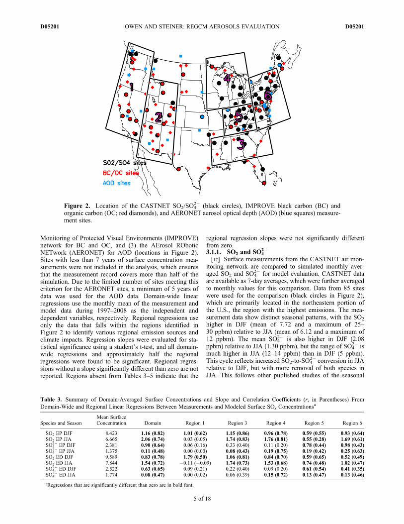
Monitoring of Protected Visual Environments (IMPROVE)network for BC and OC, and (3) the AErosol ROboticNETwork (AERONET) for AOD (locations in Figure 2).Sites with less than 7 years of surface concentration mea-surements were not included in the analysis, which ensuresthat the measurement record covers more than half of thesimulation. Due to the limited number of sites meeting thiscriterion for the AERONET sites, a minimum of 5 years ofdata was used for the AOD data. Domain-wide linearregressions use the monthly mean of the measurement andmodel data during 1997–2008 as the independent anddependent variables, respectively. Regional regressions useonly the data that falls within the regions identified inFigure 2 to identify various regional emission sources andclimate impacts. Regression slopes were evaluated for sta-tistical significance using a student’s t-test, and all domain-wide regressions and approximately half the regionalregressions were found to be significant. Regional regres-sions without a slope significantly different than zero are notreported. Regions absent from Tables 3–5 indicate that the

regional regression slopes were not significantly differentfrom zero.3.1.1. SO2 and SO4

2�

[17] Surface measurements from the CASTNET air mon-itoring network are compared to simulated monthly aver-aged SO2 and SO4

2� for model evaluation. CASTNET dataare available as 7-day averages, which were further averagedto monthly values for this comparison. Data from 85 siteswere used for the comparison (black circles in Figure 2),which are primarily located in the northeastern portion ofthe U.S., the region with the highest emissions. The mea-surement data show distinct seasonal patterns, with the SO2

higher in DJF (mean of 7.72 and a maximum of 25–30 ppbm) relative to JJA (mean of 6.12 and a maximum of12 ppbm). The mean SO4

2� is also higher in DJF (2.08ppbm) relative to JJA (1.30 ppbm), but the range of SO4

2� ismuch higher in JJA (12–14 ppbm) than in DJF (5 ppbm).This cycle reflects increased SO2-to-SO4

2� conversion in JJArelative to DJF, but with more removal of both species inJJA. This follows other published studies of the seasonal

Figure 2. Location of the CASTNET SO2/SO42� (black circles), IMPROVE black carbon (BC) and

organic carbon (OC; red diamonds), and AERONET aerosol optical depth (AOD) (blue squares) measure-ment sites.

Table 3. Summary of Domain-Averaged Surface Concentrations and Slope and Correlation Coefficients (r, in Parentheses) FromDomain-Wide and Regional Linear Regressions Between Measurements and Modeled Surface SOx Concentrations

a

Species and SeasonMean SurfaceConcentration Domain Region 1 Region 3 Region 4 Region 5 Region 6

SO2 EP DJF 8.423 1.16 (0.82) 1.01 (0.62) 1.15 (0.86) 0.96 (0.78) 0.59 (0.55) 0.93 (0.64)SO2 EP JJA 6.665 2.06 (0.74) 0.03 (0.05) 1.74 (0.83) 1.76 (0.81) 0.55 (0.28) 1.69 (0.61)SO4

2� EP DJF 2.381 0.90 (0.64) 0.06 (0.16) 0.33 (0.40) 0.11 (0.20) 0.78 (0.44) 0.98 (0.43)SO4

2� EP JJA 1.375 0.11 (0.48) 0.00 (0.00) 0.08 (0.43) 0.19 (0.75) 0.19 (0.42) 0.25 (0.63)SO2 ED DJF 9.589 0.83 (0.78) 1.79 (0.50) 1.06 (0.81) 0.84 (0.70) 0.59 (0.65) 0.52 (0.49)SO2 ED JJA 7.844 1.54 (0.72) �0.11 (�0.09) 1.74 (0.73) 1.53 (0.68) 0.74 (0.48) 1.02 (0.47)SO4

2� ED DJF 2.522 0.63 (0.65) 0.09 (0.21) 0.22 (0.40) 0.09 (0.20) 0.61 (0.54) 0.41 (0.35)SO4

2� ED JJA 1.774 0.08 (0.47) 0.00 (0.02) 0.06 (0.39) 0.15 (0.72) 0.13 (0.47) 0.13 (0.46)

aRegressions that are significantly different than zero are in bold font.


5 of 18

cycle of SO42�, with greater concentrations in summer than

winter over most of the United States [Malm et al., 2004;Jaffe et al., 2005; Luo et al., 2011].[18] In DJF, the EP simulation captures the general spatial

pattern of SO2 and SO42�, with relatively high concentrations

in the eastern portion of the U.S. and relatively low con-centrations in the western U.S. (Figures 3a and 3c andFigures 4a and 4c). The modeled SO2 is biased slightly high(16%) relative to the measurements with concentrationscentered around the regression line, while the modeled SO4

2�

is biased slightly low (10%, Table 3). In JJA, however, theEP simulation fails to reproduce the observed concentra-tions, where SO2 is overestimated by 106%. While the sta-tistical mean EP SO2 is similar to the statistical meanmeasured concentrations, maximum simulated SO2 con-centrations are more than three times higher than the maxi-mum measured concentrations. In contrast to the SO2, theSO4

2� is underestimated by 90%. Similar to SO2, meanconcentrations are similar but the maximum modeled SO4

2�

is a factor of 2.5 lower than the maximum measured SO42�.

These biases also suggest incomplete conversion of SO2 tosulfate in the model, as noted in other RegCM studies [e.g.,Solmon et al., 2006] where it was attributed to an underes-timate of the gaseous conversion by OH and the lack ofaqueous production via O3 reduction. Despite the differ-ences in SO2 emissions between the EPA and EDGARinventories, the ED simulation of SO2 and SO4

2� is quitesimilar to the EP simulation. As with EP, the DJF ED sim-ulation compares well with observations, and are 17% lowerfor SO2 and 37% lower than observed for SO4

2�. In JJA, thesame pattern of high SO2 and low SO4

2� is present in the EDsimulation, again suggesting the incomplete chemical con-version of SO2 to SO4

2�.[19] The seasonal changes in the model sulfate biases (e.

g., stronger biases in JJA than DJF and the consistent over-estimation of SO2 and underestimation of SO4

2�) suggestsincomplete chemical conversion in the model, as notedabove. To explore the sulfate conversion, the total sulfur

contributed by each species (Figures 5a and 5b) and the ratioof SO2 to SO4

2� (not shown) were also examined. Theregression of modeled versus the measured total sulfur areremarkably similar in both seasons, with the ED low by 10–17% and the EP high by 15–22%, reflecting the DJFregressions for SO2 and the nature of high-resolution pointsources in the EP inventory. These results support the con-clusion that the emission inventories capture the SO2 emis-sions fairly well. The comparison of modeled and measuredSO2/SO4

2� ratios, however, are starkly different in eachseason and show that the ratio of SO2/SO4

2� is much higherthan it should be in JJA. These observations support thehypothesis that the sulfate conversion likely contributes tothe JJA model bias.[20] An examination of the domain-averaged column

profiles for SO2 and SO42� shows that vertical mixing could

also play a role in the surface model biases. Vertical profilesshow higher concentrations aloft (greater than 0.9 sigma,approximately 870 mb) in JJA than DJF, suggesting anincrease in summer vertical mixing (Figures 6a and 6b).Surface SO2 and SO4

2� concentrations are greater in DJFthan JJA for both ED and EP simulations, and as notedabove, are close in magnitude despite the ED emissionsbeing approximately 20% higher. However, ED concentra-tions of sulfate are higher than EP aloft particularly in thesummer, reflecting the increased ED emission inventory.This behavior suggests that part of the model bias could bedue to the excessive vertical mixing in the model, whichcould reduce surface concentrations through strong mixing.[21] Finally, the vertical profile and sulfate column burden

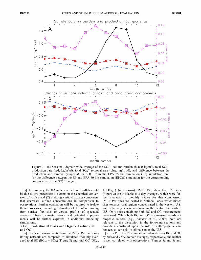
is also important for understanding the climate effects ofsulfate. The domain-average total SO4

2� column burden(Figure 7a) shows a strong seasonal cycle and peaks inAugust and September. Total column sulfate productionoutweighs removal throughout the year, leading to anincrease in net sulfate production in the early summer and anincrease in column burden in late summer. However, due tothe increase in vertical mixing and higher winds aloft, there

Table 4. Summary of Domain-Averaged Surface Concentrations and Slope and Correlation Coefficients (r, in Parentheses) FromDomain-Wide and Regional Linear Regressions Between Measurements and Modeled Surface Black and Organic Carbon Concentrationsa

Species and SeasonMean SurfaceConcentration Domain Region 1 Region 3 Region 4 Region 5 Region 6

BC EP DJF 0.191 0.42 (0.56) 0.08 (0.26) �0.01 (�0.05) 0.43 (0.44) 0.55 (0.61) 0.34 (0.69)BC EP JJA 0.163 0.22 (0.43) �0.01 (�0.04) 0.26 (0.68) 0.04 (0.19) 0.41 (0.60) 0.32 (0.70)BC ED DJF 0.211 0.28 (0.59) 0.09 (0.42) �0.01 (�0.07) 0.32 (0.44) 0.18 (0.49) 0.27 (0.72)BC ED JJA 0.174 0.15 (0.44) 0.01 (0.06) 0.09 (0.56) 0.04 (0.22) 0.11 (0.52) 0.26 (0.72)OC EP DJF 0.418 0.23 (0.53) 0.02 (0.08) �0.03 (�0.17) 0.16 (0.33) 0.18 (0.33) 0.20 (0.66)OC EP JJA 0.358 0.02 (0.15) �0.01 (�0.07) 0.07 (0.42) 0.00 (0.00) �0.03 (�0.10) 0.07 (0.36)OC ED DJF 0.458 0.16 (0.52) 0.05 (0.23) �0.01 (�0.06) 0.07 (0.24) 0.06 (0.28) 0.14 (0.52)OC ED JJA 0.381 0.01 (0.12) �0.00 (�0.08) 0.01 (0.14) 0.00 (�0.05) 0.00 (�0.05) 0.05 (0.30)

aRegressions that are significantly different than zero are in bold font.

Table 5. Summary of Domain-Averaged Aerosol Optical Depth (AOD) and Slope and Correlation Coefficients (r, in Parentheses) FromDomain-Wide and Regional Linear Regressions Between Measurements and Modeled AODa

Species and Season Mean AOD Domain Region 1 Region 5 Region 6

AOD EP DJF 0.114 0.68 (0.26) �0.08 (�0.34) 0.28 (0.09) 0.05 (0.02)AOD EP JJA 0.084 0.31 (0.74) 0.02 (0.09) 0.14 (0.45) 0.17 (0.47)AOD ED DJF 0.149 0.48 (0.20) �0.18 (�0.30) 0.39 (0.14) �0.01 (0.00AOD ED JJA 0.103 0.24 (0.70) �0.06 (�0.08) 0.10 (0.38) 0.18 (0.57)

aRegressions that are significantly different than zero are in bold font. Note: No AOD measurement sites were available for regions 3 and 4.


6 of 18

is a greater flux out of the model domain in the summertime,leading to a lag in the modeled column burden. In oursimulations, the gaseous conversion increases in the sum-mer, but is an order of magnitude less than the aqueousconversion (not shown). While this lack of conversion couldcreate the low JJA SO4

2�, it is likely that the increased ver-tical transport decreases the modeled surface SO4

2� as well.The vertical transport and impact on wet removal is dis-cussed further in section 4.[22] The sensitivity of the model to SO2-SO4

2� conversionand transport parameterizations has been tested in otherRegCM studies [Qian et al., 2001; Solmon et al., 2006].Qian et al. [2001] found that sulfate concentrations werepredominantly sensitive to emission sources, aqueous con-version and wet removal, with little sensitivity to gas phaseconversion and dry deposition. However, the lack of

comparison to measured sulfate in this paper does not pro-vide any quantitative information about the sulfate formationin these simulations over East Asia. Solmon et al. [2006]tested the sensitivity of aerosol aging, emission strength,and convective transport over northern Africa and Europe,finding that found increased convective mixing decreasedthe surface concentrations of SO4

2� from 5–40% in JJA.Based on these previous studies and the results found here,the implication is that the vertical transport can be animportant driver in surface concentration evaluations.Additionally, our degraded evaluations in summertimecompared to winter suggest that vertical mixing could defi-nitely affect model biases. However, the relative overesti-mate of summer SO2 and underestimate of SO4

2� points toinsufficient conversion from SO2 to SO4

2�.

Figure 3. Contours of climatological modeled SO2 concentrations for (a) DJF and (b) JJA for the EPA25 km simulation (EP). CASTNET ground-based measurement locations are indicated with circles coloredby the measured mean concentrations (right half) and corresponding modeled concentrations (left half).Monthly measured/modeled data and regression lines for the EDGAR 25 km (black), EP (red), andEPA 60-km (blue) simulations are shown for (c) DJF and (d) JJA. The 1:1 line is shown in dot-dashedgray.


7 of 18

Figure 4. Same as Figure 3, but for SO42�.

Figure 5. Monthly measured/modeled data and regression lines of the total sulfur for the EDGAR 25 km(black), EP (red), and EPA 60-km (blue) simulations are shown for (a) DJF and (b) JJA. The 1:1 line isshown in dot-dashed gray.


8 of 18

Figure 6. Domain-average vertical profiles of concentrations of (a) SO2, (b) SO42�, (c) black carbon

(BC), (d) organic carbon (OC), (e) aerosol optical depth (AOD), and (f) the specific humidity.


9 of 18

[23] In summary, the JJA under-prediction of sulfate couldbe due to two processes: (1) errors in the chemical conver-sion of sulfate and (2) a strong vertical mixing componentthat decreases surface concentrations in comparison toobservations. Further evaluation will be required to isolatethese processes, including estimates of turbulent mixingfrom surface flux sites or vertical profiles of speciatedaerosols. These parameterizations and potential improve-ments will be further explored in additional modelingsimulations.3.1.2. Evaluation of Black and Organic Carbon (BCand OC)[24] Surface measurements from the IMPROVE air mon-

itoring network are compared to simulated monthly aver-aged total BC (BChb + BChl) (Figure 8) and total OC (OChb

+ OChl ) (not shown). IMPROVE data from 79 sites(Figure 2) are available as 3-day averages, which were fur-ther averaged to monthly values for this comparison.IMPROVE sites are located in National Parks, which biasessites towards rural regions concentrated in the western U.S.with relatively sparse coverage in the central and easternU.S. Only sites containing both BC and OC measurementswere used. While both BC and OC are missing significantbiogenic sources [e.g., Jimenez et al., 2009], both arerelevant to the discussion in the following sections andprovide a constraint upon the role of anthropogenic car-bonaceous aerosols in climate over the U.S.[25] In DJF, the EP simulation underestimates BC and OC

by 58% and 77% (domain average), respectively, and neitheris well correlated with observations (Figures 8a and 8c and

Figure 7. (a) Seasonal, domain-wide average of the SO42� column burden (black; kg/m2), total SO4

2�

production rate (red; kg/m2/d), total SO42� removal rate (blue; kg/m2/d), and difference between the

production and removal (magenta) for SO42� from the EPA 25 km simulation (EP) simulation, and

(b) the difference between the EP and EPA 60 km simulation (EPC)C simulation for the correspondingcomponents of the SO4

2� budget.


10 of 18

Table 4). In JJA, the correlation between the model andmeasurements degrades significantly, particularly for OC,where there appears to be little correlation between themodeled and measured OC in JJA, which is likely caused bythe lack of biogenic organic aerosol in our model. For BC,observations during both seasons show likely biomassburning events which produce a broad range of BC con-centrations (up to 2–3 ppbm) that are not matched in themodel (simulated values typically peak at 0.5 ppbm).[26] As in the EP simulation, the ED BC and OC con-

centrations are also underestimated by the model in bothseasons. Again, the BC results are slightly skewed by theapparent absence of biomass burning events in the westernU.S., leading to reduced measured-modeled agreement.Regional results are consistent with the domain-wide results,with the exception of region 6, which maintains similarslope and fit values from DJF to JJA. The modeled OC inJJA is similarly uncorrelated to measurements by an anapparent lack of biogenic emissions.[27] For the carbonaceous aerosols, the EP inventory

results in the best measured-modeled agreement in both

seasons. It is important to note that the EP inventory onlyincludes emissions from fossil fuel combustion, therefore anincrease in agreement reflects the anthropogenic emissionsinventory component only. Interestingly, the surface con-centrations of both BC and OC are significantly higher in theEP simulations (33–40%). However, at higher altitudes,however, the two inventories are virtually identical whencomparing within a season. As noted in the sulfur compari-son, the profiles indicate greater vertical mixing in JJA,which is likely a contributing factor to the decrease inmodeled surface concentrations from DJF to JJA.[28] As with sulfur species, DJF represents a time period

when the simplified model parameterizations most accu-rately mimic reality, despite comparison statistics that sug-gest missing or underestimated sources. We conducted twoadditional sensitivity tests of the effect of emission strength,which increased BC emissions by a factor of 2.25 and OCemissions by a factor of 4.4 (the inverse of the slope for theEPC DJF regression) for a 60 km resolution simulation. Theincreased emissions substantially increased the simulatedBC and OC, however, the r was virtually unchanged. The

Figure 8. Same as Figure 3, but for black carbon (BC) using measurement data from the IMPROVEnetwork.


11 of 18

modeled values remained poorly correlated with the mea-surements, strongly suggesting that missing carbonaceoussources are likely to be the cause of the measured-modeleddiscrepancies (i.e., biomass burning and biogenic emis-sions). Additionally, the dynamic range of the measured andmodeled BC also suggests that some point sources are alsomissing from current anthropogenic inventories, as noted byFernandes et al. [2007].3.1.3. Evaluation of Aerosol Optical Depth (AOD)[29] Surface measurements of AOD from AERONET, a

network of ground-based sun photometers which measureatmospheric aerosol properties [Holben et al., 1998], arecompared with monthly averaged simulated AOD. Here, weimplement Level 2 (cloud-screened and quality assured)monthly averages from 24 sites (Figure 2). The AOD at eachtime step within RegCM is calculated from the aerosolconcentration and extinction coefficient [Solmon et al.,2006] and modeled AOD values are representative of themean AOD aggregated over the 350–640 nm spectral band.Four bands of AERONET AOD (340, 380, 440, and 500 nmspectral bands) were averaged to correspond to the modeled

AOD. The AOD offers a more complete evaluation of themodel performance, as it incorporates all aerosols speciesover the whole column. However, it is inherently limited bythe fact that these RegCM simulations only consideranthropogenic aerosols with notable missing sources such asbiomass burning, sea salt, dust, and biogenic organics.[30] The regression statistics show that AOD is generally

underestimated in both seasons and emission scenarios. InDJF, AOD is low by 32% and 53% for EP and ED,respectively (Figures 9a and 9c). In JJA, the measured AODroughly doubles, while the simulated EP AOD decreases byapproximately half, resulting in even lower regression slopesfor both emission inventories. Interestingly, however, theJJA though the r is significantly improved over DJF. Thelow modeled JJA AOD values provides further support tomissing summertime emissions and chemical conversion ofsulfate in the model (noted in sections 3.1.1–3.1.2). Verticalprofiles of AOD (Figure 6f) suggest that sulfate is the maindriver of modeled light extinction [e.g., Ginoux et al., 2006],due to similar vertical maxima in sulfate concentration andAOD at approximately 0.9 sigma (approximately 870 mb).

Figure 9. Same as Figure 3, but for aerosol optical depth (AOD) using measurement data from theAERONET network.


12 of 18

This supports an underestimate of JJA AOD as the sulfatespecies are also underestimated.

3.2. Impact on TOA Forcing

[31] Finally, we evaluate the direct effect of SO42�, BC,

and OC concentrations on the spatial top of the atmosphereradiative forcing (TOA), relative to clear sky conditions(Figure 10). TOA is calculated in the radiative transfer cal-culations as the difference in absorbed solar flux between aclear sky with no aerosols and the simulated aerosol burden.Overall, the EP and ED simulations produce similar spatialdistributions with TOA slightly higher over the Ohio RiverValley in the winter and the Eastern seaboard in the summer.Wintertime TOA is concentrated in the East Coast, withforcing increasing throughout the continent in the summer.

Seasonal domain-averaged TOA (Figure 11) shows that thewinter forcing is almost identical between EP and ED.[32] However, in the summer and fall, the ED TOA

increases over the EP TOA by more than 1 Wm�2. This isin accordance with greater SO2 emissions in the ED inven-tory and increased sulfate conversion in the summer, leadingto greater sulfate concentrations throughout the verticalprofile and slightly higher AOD values (Figure 6). While theatmospheric dynamics are unchanged between these twosimulations, the greater concentrations in ED profile areamplified in the summer due to the increase in summertimeconvective mixing and summer sulfate chemical conversion.The spatial distribution of the surface radiative forcing(SRF), which is also considered in climate simulations, isnearly identical to the TOA and slightly larger in magnitude,with SRF forcings of 15 Wm�2 (4–5 Wm�2 greater than the

Figure 10. Spatial distribution of top of the atmosphere radiative forcing (TOA) for the EDGAR 25 km(ED; Figures 10a and 10d), EPA NEI 25 km (EP; Figures 10b and 10e), and EPA NEI 60 km (EPC;Figures 10c and 10f) simulations for (a–c) DJF and (d–f) JJA.

Figure 11. Domain and seasonal average of the top of the atmosphere radiative forcing (TOA) forEDGAR 25 km (ED; black), EPA NEI 25 km (EP;red), and EPA NEI 60 km (EPC; blue) simulations.


13 of 18

TOA). In contrast to the analysis of species concentrations,these results suggest that the climate impact of the emissionsinventory resolution can have an impact on the aerosol TOA,particularly in the summer when chemical conversion andconvective mixing are more active. However, as discussed inthe next section, the model resolution itself may play anequally large role at introducing uncertainty into climatemodel calculations.

4. Evaluation of the Effect of ClimateModel Resolution

[33] In addition to the impact of emission inventory onprecipitation and TOA, we evaluate the impact of climatemodel resolution by comparing the fine-scale 25 km reso-lution simulation (EP) with a coarse resolution (60 km; EPC)simulation using the same 4 km EPA emissions inventory.For individual aerosol species, the differences between thedomain-wide regressions for EP and EPC were relativelysmall (within 7% in DJF and 28% in JJA) with slightlyimproved regression statistics in the EPC simulation.Despite regression similarities, EPC SO2 and SO4

2� con-centrations are greater than the EP in both seasonsthroughout the full vertical profile (e.g., Figure 6b, DJF, themean SO4

2� surface concentration increases from 0.46 ppbmin EP to 0.65 ppbm in EPC). BC and OC concentrations arealso higher in EPC in the lower troposphere, with greaterdifferences in the summer than the winter. AOD is alsohigher in EPC, with the mean AOD increasing by 0.035 inDJF and by 0.019 in JJA. Because these two simulations are

using the same emission inventories, the concentration andAOD differences are due to different physical processes inthe model caused by changes in model resolution. Specifichumidity profiles show that the vertical column in the EPCsimulation is drier than the EP simulation in both seasons(Figure 6f), suggesting that it is not a relative humidityenhancement of the aerosol scattering.[34] We note that these simulations do not include the

aerosol indirect effect, and the primary differences in thevertical profile of specific humidity are due to changes inthe climate model resolution.[35] Differences in the sulfate budget (Figure 7b) suggest

that the removal processes could be driving the concentra-tion differences in the EP and EPC simulations. The EPCtotal sulfate burden is greater than EP, with lower productionand removal rates in the EPC simulation. Additionally, thenet production (e.g., total production rate - total removalrate) for the EPC simulation is greater than the EP simula-tion, leading to less aerosol removal and hence a greateraerosol burden in the EPC simulation. Because removal ratesappear to be a key difference between the EP and EPCsimulations and wet removal is the dominant aerosol sink,we examine the precipitation variations between the twosimulations.[36] Figure 12a shows the seasonal cycle of total precipi-

tation for the EP and EPC simulations as compared to grid-ded precipitation observations from the Climatic ResearchUnit (CRU) [Mitchell and Jones, 2005]. In general, the EPCsimulates less total precipitation than the EP simulation,typically improving agreement with observations in the

Figure 12. (a) Domain-averaged total precipitation for the observed CRU data set (black solid line), EP(red dotted line), and EPC (blue dashed line) simulations. (b) Domain-averaged convective precipitation(no symbols) and large-scale precipitation (diamonds) from EP (red) and EPC (blue) simulations.


14 of 18

winter. From the seasonal perspective, the large-scalescheme dominates in the winter with nearly equal contribu-tions of large-scale and convective precipitation in thesummer (Figure 12b). Typically, the EPC simulates moreconvective precipitation in the summer and consistentlysimulates less large-scale precipitation throughout the sea-sonal cycle (Table 6). These results are consistent with otherstudies from both regional [Leung and Qian, 2003; Gaoet al., 2006; Rauscher et al., 2010] and global [Fang et al.,2011] models, which find that precipitation tends toincrease with an increase in resolution, and is often due to adecrease in the convective precipitation and compensatingincreases in large-scale precipitation [Rauscher et al., 2010;Duffy et al., 2003]. However, the EPC simulation reducesthe precipitation bias in DJF, suggesting that the fine reso-lution simulation may be overestimating the large-scalecontribution of precipitation to the total (Table 6). The large-scale precipitation parameterization is developed frommeasured-modeled evaluations implementing a 60 kmRegCM resolution [Pal et al., 2000], therefore we couldexpect that climate model simulations with similar resolu-tions in the parameterization development may lead to lowermodel biases. While it is possible that differences in aerosolconcentrations are driving changes in precipitation, ourevaluation of the EP versus ED suggests that changes inresolution is the primary driver of changes in precipitationbetween the simulations.[37] The decrease in EPC precipitation increases aerosol

concentrations and increases TOA for the EPC simulationthroughout the seasonal cycle (Figure 11). The domain-average TOA for the EPC simulation is 0.08 W m�2 greaterthan the EP simulation, with local differences of up to 5 Wm�2 in the eastern U.S. Unlike the differences between theED and EP simulations, which were typically in the sum-mertime and likely driven by differences in the emissionsand chemical conversion, the difference between the EP andEPC forcing is likely driven by changes in wet removalprocesses.[38] To explore the sensitivity of our results to the pre-

cipitation parameterizations, we conducted one set of sensi-tivity tests using an alternative closure option for the Grellconvective scheme (changing from the Fritsch-Chappellclosure to the Arakawa-Schubert closure). The set includes a3-year simulation at 25 km and one at 60 km. In general, thechange in closure scheme caused a 2–4% decrease in thetotal precipitation, with small changes in the large-scaleprecipitation (�1%) and greater changes in the convectiveprecipitation (6–26%). The decreases in the total and large-scale precipitation in the coarser model resolution (60 km) is

very similar to our original results. For the convective pre-cipitation, the results are more variable, with an overalldecrease in the convective precipitation. Because the large-scale precipitation is the greatest controller of wet deposition(large-scale removal was approximately 25 times greaterthan convective removal in our simulations), we do notexpect that this difference in convective precipitation willsubstantially alter our conclusions about the impact of large-scale precipitation on aerosol wet removal. Indeed, changesin the the column burden and TOA in sensitivity tests fol-lows the same pattern seen in the EP and EPC simulations,with a greater impact on the column burden and TOA in thecoarse simulations. In addition to model physics, precipita-tion can be sensitive to land surface scheme selection,depending on the time of year and location [Tawfik andSteiner, 2011]. However, the region with the greatest aero-sol burden is not in a strongly land-atmosphere regiontherefore we do not expect that the aerosol burden would beparticularly sensitive to the land surface scheme selection.[39] To summarize, the EPC simulations have higher

concentrations of all aerosols species (SO42�, BC, OC) and

AOD in both the surface layer and lower troposphere. Theincreased SO4

2� is particularly pronounced in the summer,where mean SO4

2� concentrations in EPC can exceed EP by0.2 ppbm. Due to the apparent scale-dependence of theprecipitation parameterizations, EP simulates more large-scale precipitation than EPC in the summer, which leads to alarge removal of aerosol in the EP simulation. In general,wet deposition is the dominant mechanism of sulfateremoval in the atmosphere, and the increased precipitation inthe EP simulation over the EPC simulation results in 16%more wet deposition in EP. While there are differences in theconvective and large-scale balance of precipitation withinthe domain, most of the change in wet deposition can beattributed to the magnitude of large-scale precipitation.Based on comparisons with total CRU precipitation, theEPC results provide an improved measured-modeled agree-ment suggesting that the EPC processes (and higher surfaceforcings) are likely more realistic. Additionally, the EPCaerosol species regression statistics are slightly better thanthe EP simulations (Table 5 and Figure 9), suggesting thatthe EPC precipitation more accurately represents wet depo-sition processes.

5. Discussion and Conclusions

[40] The regional climate model RegCM was used to todetermine the importance of the resolution of an emissioninventory versus the resolution of the model grid on the

Table 6. Precipitation Averaged by Region and Season for the EP and EPC Simulations and the CRU Data Set (mm/month)

Species/Season Domain Region 1 Region 2 Region 3 Region 4 Region 5 Region 6

Precip CRU all 61.40 56.21 26.98 113.89 70.18 100.77 94.11Precip EP all 68.47 83.95 53.97 101.54 78.08 93.31 96.10Precip EPC all 63.81 74.72 46.34 102.59 79.70 97.69 97.65Precip CRU DJF 51.96 85.47 17.95 140.27 55.47 128.56 87.76Precip EP DJF 66.56 138.44 52.43 98.52 74.57 98.13 103.50Precip EPC DJF 61.36 125.03 49.71 99.97 73.98 89.47 91.88Precip CRU JJA 73.06 47.11 27.81 145.04 71.67 132.72 77.20Precip EP JJA 75.61 60.85 42.45 139.55 90.29 112.36 106.95Precip EPC JJA 69.45 53.93 37.68 169.58 78.55 134.55 106.79


15 of 18

climate forcing of anthropogenic aerosols over the U.S.RegCM was used to simulate the climate impact of SO2/SO4

2�, BC and OC over the U.S. from 1997–2008. Threesimulations were completed, one with a 25 km model gridusing the 1° � 1° EDGAR anthropogenic aerosol emissioninventory, another 25 km simulation, but with the EPA’sNEI 4 � 4 km emission inventory and a third with with theEPA NEI inventory, but at a 60 km model grid. The modelperformance was evaluated against surface measurements ofthe species concentrations, AOD, and precipitation.[41] The comparisons of the two emissions inventories

(EPA versus EDGAR) showed small differences in primaryemissions (SO2, BC and OC typically within 15%) and theresulting modeled concentrations. Model SO2 and SO4

2�

results for ED and EP compare well to concentrations andAOD observations in winter, suggesting that emissioninventories sufficiently capture most major sources. How-ever, the measurement/model agreement was reduced in thesummer with an overestimation of SO2 and underestimationof SO4

2�, indicating insufficient conversion of SO2 to SO42�

in accordance with previous findings [Solmon et al., 2006].For BC, the EP surface concentrations were closer toobservations than ED BC surface concentrations, thoughboth inventories underestimated BC by 58% (72%) for EP(ED) in DJF and by 78% (85%) in JJA. A sensitivity test ofthe magnitude of the BC emissions indicated that the EPAinventory is missing BC sources, particularly in the summertime, likely due to the lack of biomass burning in theinventory. Surface OC concentrations in both EPA andEDGAR simulations were underestimated by 77% in DJFand 98% in JJA, likely due to the lack of biogenic organics.Finally, the EP simulation slightly improved measured-modeled agreement for AOD compared to the ED simula-tion. Because the majority of the modeled AOD is driven bythe SO4

2�, the lack of summertime SO42� and OC contribute

to the AOD underestimates in JJA. Overall, the EP simula-tions consistently showed marginal improvement based onmeasured-modeled metrics as compared to the ED simula-tions, though the improvements were not as large as thedifference in the magnitude of emissions. Despite similari-ties in the surface aerosol concentrations, differences in theJJA climate response is notable between the two inventories.The ED inventory leads to slightly higher sulfate con-centrations throughout the vertical profile, which leads toan increased TOA for the EDGAR inventory in thesummertime.[42] Comparisons of the 25 km (EP) and 60 km (EPC)

simulations show than a decrease in resolution increasessurface concentrations of all species, leading to an increasedaerosol burden and TOA forcing of about 2.5 Wm�2 in JJA.The resolution-driven change in the magnitude of JJA TOAforcing is similar to the change caused by different emis-sions inventories. For all aerosol species (SO4

2�, BC andOC), the EPC simulation provides better agreement withobservations than the EP simulation due to higher con-centrations of these species throughout most of the lowertroposphere. Vertical profiles of AOD (Figure 9e) indicatethat most of the extinction is due to the sulfate aerosol, andEPC SO4

2� concentrations are substantially larger than theEP concentrations throughout the vertical profile. Anexamination of the sulfate budget shows that while moreSO2-to-SO4

2� conversion is occurring in the EP simulation,

the differences in the two simulations are driven by the lossprocesses, notably the wet deposition due to large-scaleprecipitation. Less deposition in the coarse simulations resultin higher sulfate concentrations throughout the vertical pro-file, leading to greater extinction and higher surface forcings.Because the precipitation biases are reduced in the EPCsimulations, the coarse scale estimation of precipitation andwet removal may provide a better estimate of present-dayclimate.[43] In conclusion, evaluations of modeled aerosol con-

centrations, AOD and precipitation suggest that that climatemodel resolution and emissions inventory can have animportant impact on modeled aerosol forcings via scale-dependent precipitation parameterizations. Our results findthat wet removal of aerosols is very dependent on the ratio ofconvective and large-scale precipitation simulated by themodel. As we note above, many of these parameterizationsare tuned for specific resolution, and changing resolutionwithout precipitation tuning may lead to large changes in theaerosol burden. Therefore, when considering changes inmodel resolution, the precipitation parameterizations play akey role in regional simulations of atmospheric aerosols andchemistry-climate feedbacks. These findings are relevant forother atmospheric pollutants and global scale models as well[e.g., Fang et al., 2011]. While there are clearly manyshortcomings in these simulations, notably the absence ofbiomass burning emissions and secondary organic aerosolformation, the results suggest a scale dependence that hasnot been closely examined in the literature. Because thedifferences in the precipitation ultimately affect the com-puted surface forcings, selection of model resolution mayhave a greater impact on surface forcing than the selection ofthe emissions inventory and missing emission sources.These results suggest that future climate model studiesshould carefully examine scale-dependent precipitationprocesses, particularly those related to precipitation and wetremoval, as these processes strongly affect aerosol con-centrations and resulting surface forcings.

[44] Acknowledgments. We thank Ahmed Tawfik (University ofMichigan), Fabien Solmon (ICTP), Ashraf Zakey (DMI), and the ICTPRegCNET for providing simulation support on RegCM simulations. Addi-tionally, we gratefully acknowledge MOZART boundary conditions pro-vided by Louisa Emmons (NCAR). Measurement data were provided bythe CASTNET, IMPROVE, and AERONET data networks, and we thankthe network supporters for providing this data to the public. We thank GregFrost and Stuart McKeen for processed NEI inventories prepared from EPAemissions files. Finally, we wish to thank the three reviewers, who provideda thorough review and many comments which helped improve the qualityof this paper.

ReferencesAppel, K. W., K. M. Foley, J. O. Bash, R. W. Pinder, R. L. Dennis, D. J.Allen, and K. Pickering (2010), A multi-resolution assessment of theCommunity Multiscale Air Quality (CMAQ) Model v4.7 wet depositionestimates for 2002–2006, Geosci. Model Dev. Discuss., 3(4), 2315–2360,doi:10.5194/gmdd-3-2315-2010.

Bian, H., M. Chin, J. M. Rodriguez, H. Yu, J. E. Penner, and S. Strahan(2009), Sensitivity of aerosol optical thickness and aerosol direct radia-tive effect to relative humidity, Atmos. Chem. Phys., 9(7), 2375–2386,doi:10.5194/acp-9-2375-2009.

Bond, T. C., E. Bhardwaj, R. Dong, R. Jogani, S. Jung, C. Roden,D. Streets, S. Fernandes, and N. Trautmann (2007), Historical emissionsof black and organic carbon aerosol from energy-related combustion,1850–2000, Global Biogeochem. Cycles, 21, GB2018, doi:10.1029/2006GB002840.


16 of 18

Cooke, W. F., C. Liousse, H. Cachier, and J. Feichter (1999), Constructionof a 1° � 1° degree fossil fuel emission data set for carbonaceous aerosoland implementation and radiative impact in the echam4 model, J. Geo-phys. Res., 104, 22,137–22,162.

Duffy, P. B., B. Govindasamy, J. P. Iorio, J. Milovich, K. R. Sperber,K. E. Taylor, M. F. Wehner, and S. L. Thompsonn (2003), High-resolution simulations of global climate, part 1: present climate, Clim.Dyn., 19, 371–390.

Ekman, A., and H. Rodhe (2003), Regional temperature response due toindirect sulfate aerosol forcing: impact of model resolution, Clim. Dyn.,21, 1–10, doi:10.1007/s00382-003-0311-y.

Emmons, L. K., et al. (2010), Description and evaluation of the Model forOzone and Related chemical Tracers, version 4 (MOZART-4), Geosci.Model Dev., 3(1), 43–67, doi:10.5194/gmd-3-43-2010.

Fang, Y., et al. (2011), The impacts of changing transport and precipitationon pollutant distributions in a future climate, J. Geophys. Res., 116,D18303, doi:10.1029/2011JD015642.

Fernandes, S. M., N. M. Trautmann, D. G. Streets, C. Roden, and T. Bond(2007), Global biofuel use, 1850–2000, Global Biogeochem. Cycles, 21,GB2019, doi:10.1029/2006GB002836.

Frost, G. J., et al. (2006), Effects of changing power plant NOx emissions onozone in the eastern United States: Proof of concept, J. Geophys. Res.,111, D12306, doi:10.1029/2005JD006354.

Gao, X., J. S. Pal, and F. Giorgi (2006), Projected changes in mean andextreme precipitation over the Mediterranean region from a high resolu-tion double nested RCM simulation, Geophys. Res. Lett., 33, L03706,doi:10.1029/2005GL024954.

Ginoux, P., L. W. Horowitz, V. Ramaswamy, I. V. Geogdzhayev, B. H.Holben, G. Stenchikov, and X. Tie (2006), Evaluation of aerosol distribu-tion and optical depth in the Geophysical Fluid Dynamics Laboratorycoupled model for CM2.1 for present climate, J. Geophys. Res., 111,D22210, doi:10.1029/2005JD006707.

Giorgi, F. (1989), Two-dimensional simulations of possible mesoscaleeffects of nuclear war fires. I: model description, J. Geophys. Res., 94,1127–1144.

Giorgi, F., and W. L. Chameides (1986), Rainout lifetimes of highly solubleaerosols and gases as inferred from simulations with a general circulationmodel, J. Geophys. Res., 91, 14,367–14,376.

Giorgi, F., X. Bi, and Y. Qian (2002), Direct radiative forcing and regionalclimatic effects of anthropogenic aerosols over East Asia: A regional cou-pled climate-chemistry/aerosol model study, J. Geophys. Res., 107(D20),4439, doi:10.1029/2001JD001066.

Grell, G. A. (1993), Prognostic evaluation of assumptions used by cumulusparameterizations, Mon. Weather Rev., 121, 764–787.

Grell, G. A., J. Dudhia, and D. R. Stauffer (1994), A description of the fifth-generation Penn State-NCAR Mesoscale Model (MM5), NCAR Tech.Note NCAR/TN-398+STR, 122 pp., Natl. Cent. for Atmos. Res., Boulder,Colo.

Hansen, J., M. Sato, P. Kharecha, G. Russell, D. W. Lea, and M. Siddall(2007a), Climate change and trace gases, Philos. Trans. R. Soc. A, 365(1856), 1925–1954, doi:10.1098/rsta.2007.2052.

Hansen, J., et al. (2007b), Climate simulations for 1880–2003 with GISSmodelE, Clim. Dyn., 29, 661–696, doi:10.1007/s00382-007-0255-8.

Holben, B., et al. (1998), AERONET—A federated instrument network anddata archive for aerosol characterization, Remote Sens. Environ., 66(1),1–16, doi:10.1016/S0034-4257(98)00031-5.

Holtslag, A. A. M., E. I. F. de Bruijin, and H. L. Pan (1990), A high reso-lution air mass transformation model for short-range weather forecasting,Mon. Weather Rev, 118, 1561–1575.

Intergovernmental Panel on Climate Change (IPCC) (2007), ClimateChange 2007: The Physical Science Basis. Contribution of WorkingGroup I to the Fourth Assessment Report of the Intergovernmental Panelon Climate Change, Cambridge Univ. Press, New York.

Jaffe, D., S. Tamuraa, and J. Harrisb (2005), Seasonal cycle and composi-tion of background fine particles along the west coast of the US, Atmos.Environ., 39, 297–306.

Jimenez, J. L., et al. (2009), Evolution of organic aerosols in the atmo-sphere, Science, 326, 1525–1529.

Kalnay, E., et al. (1996), The NCEP/NCAR 40-year reanalysis project, Bull.Am. Meteorol. Soc., 77, 437–471.

Kasibhatla, P., W. L. Chameides, and J. S. John (1997), A three dimen-sional global model investigation of seasonal variation in the atmosphericburden of anthropogenic sulfate aerosols, J. Geophys. Res., 102, 3737–3759.

Kiehl, J. T., J. J. Hack, G. B. Bonan, B. A. Boville, B. P. Briegleb,D. Williamson, and P. Rasch (1996), Description of the NCAR Commu-nity Climate Model (CCM3), NCAR Tech. Note NCAR/TN-420+STR,152 pp., Natl. Cent. for Atmos. Res., Boulder, Colo.

Kim, S.-W., et al. (2009), NO2 columns in the western United Statesobserved from space and simulated by a regional chemistry model andtheir implications for NOx emissions, J. Geophys. Res., 114, D11301,doi:10.1029/2008JD011343.

Lawrence, P. J., and T. N. Chase (2007), Representing a new MODIS con-sistent land surface the Community Land Model (CLM 3.0), J. Geophys.Res., 112, G01023, doi:10.1029/2006JG000168.

Leung, L. R., and Y. Qian (2003), Changes in seasonal and extreme hydro-logic conditions of the Georgia Basin/Puget Sound in an ensembleregional climate simulation for the mid-Century, Can. Water Resour.,28, 605–632.

Luo, C., Y. Wang, S. Mueller, and E. Knipping (2011), Diagnosis of anunderestimation of summertime sulfate using the Community MultiscaleAir Quality model, Atmos. Environ., 45, 5119–5130.

Malm, W. C., B. A. Schichtel, M. L. Pitchford, L. L. Ashbaugh, and R. A.Eldred (2004), Spatial and monthly trends in speciated fine particleconcentration in the United States, J. Geophys. Res., 109, D03306,doi:10.1029/2003JD003739.

Matsui, T., and R. A. Pielke (2006), Measurement-based estimation ofthe spatial gradient of aerosol radiative forcing, Geophys. Res. Lett., 33,L11813, doi:10.1029/2006GL025974.

Mitchell, T. D., and P. D. Jones (2005), An improved method of construct-ing a database of monthly climate observations and associated high-resolution grids, Int. J. Climatol., 25, 693–712.

National Research Council (2005), Radiative Forcing of Climate Change:Expanding the Concept and Addressing Uncertainties, Natl. Acad. Press,Washington, D. C.

Olivier, J., J. A. V. Aardenne, F. Dentene, L. Ganzeveld, and J. Peters(2005), Recent trends in global greenhouse gas emissions: Regional trendsand spatial distribution of key sources, in Non-CO2 Greenhouse Gases(NCGG-4), edited by A. van Amstel, pp. 325–330, Millpress, Rotterdam,Netherlands.

Pal, J. S., E. E. Small, and E. A. B. Eltahir (2000), Simulation of regional-scalewater and energy budgets: Representation of subgrid cloud and pre-cipitation processes within regcm, J. Geophys. Res., 105, 579–594.

Pal, J. S., et al. (2009), The ICTP RegCM3 and RegCNET: Regional cli-mate modeling for the developing world, Bull. Am. Meteorol. Soc., 88,1395.

Park, R. J., D. J. Jacob, M. Chin, and R. V. Martin (2003), Sources ofcarbonaceous aerosols over the United States and implications fornatural visibility, J. Geophys. Res., 108(D12), 4355, doi:10.1029/2002JD003190.

Qian, Y., and F. Giorgi (1999), Interactive coupling of regional climateand sulfate aerosol models over eastern Asia, J. Geophys. Res., 104,6477–6499.

Qian, Y., F. Giorgi, and Y. Huang (2001), Regional simulation of anthropo-genic sulfur over east Asia and its sensitivity to model parameters, Tellus,Ser. B, 53, 171–191.

Qian, Y., W. I. Gustafson Jr., and J. D. Fast (2010), An investigation ofthe sub-grid variability of trace gases and aerosols for global climatemodeling, Atmos. Chem. Phys., 10(14), 6917–6946, doi:10.5194/acp-10-6917-2010.

Ramanathan, V., et al. (2005), Atmospheric brown clouds: Impactson South Asian climate and hydrological cycle, Proc. Natl. Acad. Sci.U. S. A., 102, 5326–5333.

Rasch, P. J., M. Barth, J. T. Kiehl, C. M. Benkovitz, and S. E. Schwartz(2000), A description of the global sulfur cycle and its controlling pro-cesses in the National Center for Atmospheric Research Community Cli-mate Model, J. Geophys. Res., 105, 1367–1385, doi:10.1029/1999JD900777.

Rauscher, S., E. Coppola, C. Piani, and F. Giorgi (2010), Resolution effectson regional climate model simulations of seasonal precipitation overEurope, Clim. Dyn., 35, 685–711, doi:10.1007/s00382-009-0607-7.

Reynolds, R. W., N. A. Rayner, T. M. Smith, D. C. Stokes, and W. Q. Wang(2002), An improved in situ and satellite SST analysis for climate,J. Clim., 15, 1609–1625.

Shindell, D., and G. Faluvegi (2009), Climate response to regional radiativeforcing during the twentieth century, Nat. Geosci., 2, 294–300,doi:10.1038/ngeo473.

Shindell, D., H. Levy, M. D. Schwarzkopf, L. W. Horowitz, J.-F. Lamarque,and G. Faluvegi (2008), Multimodel projections of climate changefrom short-lived emissions due to human activities, J. Geophys. Res.,113, D11109, doi:10.1029/2007JD009152.

Solmon, F., F. Giorgi, and C. Liousse (2006), Aerosol modellingfor regional climate studies: Application to anthropogenic particles andevaluation over a European/African domain, Tellus, Ser. B, 58, 51–72.

Steiner, A. L., J. S. Pal, S. A. Rauscher, J. L. Bell, N. S. Diffenbaugh,A. Boone, L. C. Sloan, and F. Giorgi (2009), Land surface coupling in


17 of 18

regional climate simulations of the West African monsoon, Clim. Dyn.,98, 293–314, doi:10.1007/s00382-009-0543-6.

Stroud, C. A. et al. (2010), Impact of model grid spacing on regional- andurban-scale air quality predictions of organic aerosol, Atmos. Chem.Phys., 10(12), 30,347–30,379.

Tan, Q., Y. Huang, and W. L. Chameides (2002), Budget and export ofanthropogenic SOx from east Asia during continental outflow conditions,J. Geophys. Res., 107(D13), 4167, doi:10.1029/2001JD000769.

Tawfik, A., and A. Steiner (2011), The role of soil ice in land-atmospherecoupling over the United States: A soil moisture-precipitation winterfeedback mechanism, J. Geophys. Res., 116, D02113, doi:10.1029/2010JD014333.

U.S. Environmental Protection Agency (2011), Inventory of U.S. green-house gas emissions and sinks: 1990–2009, Tech. Rep. EPA 430-R-11-005, Washington, D. C.

van Aardenne, J. A., F. Dentener, J. Olivier, and J. Peters (2005), TheEDGAR 3.2 Fast Track 2000 dataset (32FT2000), technical report, Inst.for Environ. and Sustainability, Joint Res. Cent., Ispra, Italy.

Walker, M., and N. Diffenbaugh (2009), Evaluation of high-resolutionsimulations of daily-scale temperature and precipitation over the UnitedStates, Clim. Dyn., 33, 1131–1147, doi:10.1007/s00382-009-0603-y.

Wild, O., and M. J. Prather (2006), Global tropospheric ozone modeling:Quantifying errors due to grid resolution, J. Geophys. Res., 111,D11305, doi:10.1029/2005JD006605.

R. C. Owen, Michigan Tech Research Institute, Michigan TechnologicalUniversity, Ann Arbor, MI 48105, USA. ([email protected])A. L. Steiner, Department of Atmospheric, Oceanic, and Space Sciences,

University of Michigan, Ann Arbor, MI 48105, USA. ([email protected])


18 of 18

Documents

Effect of emissions inventory versus climate model