Embed Size (px)
Citation preview

EFFECT OF EXCHANGE RATE CHANGES ON IMPORTANT ECONOMIC
INDICATORS ON THE EXAMPLE OF ROMANIA
Ekaterina Tertyshnaya, Tregub I.V.
Financial University under the Government of the Russian Federation
1) Introduction and Formulation of the problem
The reasons underlying this theme are related to timeliness and importance of the
problem through the solutions needed to be implemented by domestic monetary policy, given the
interdependence of global financial systems. The topicality is revealed through the following
issues: first, the exchange rate is a macroeconomic indicator with remarkable effects on the
stability of the banking system, because currency depreciation has negative repercussions on the
quality of loan portfolio, and secondly, is one of the nominal convergence indicators required by
the accession to the euro area.
The exchange rate is a dynamic variable, whose mobility is determined by a wide range
of economic, financial, political and social factors ,the most important being the following GDP,
inflation rate, balance of payments and interest rates.
This paper is structured in the following way: section two entitled “The description and
evolution of key macroeconomic indicators in Romania between 2000 and 2011” presents a short
numerical and descriptive evolution of the following indicators in Romania: GDP, inflation rate,
reference interest rate and balance of payment, during 2000-2011 period. In section three
“Econometric Model. Results” we examined, using MS Word, the influence of these indicators
on exchange rate of the Romanian leu against the most important currency (EUR). The research
goal was identifying a connection, setting the intensity of the relationship among there
indicators, determining the parameters of the regression equation and testing the validity of the
model. The study ends with some conclusions.
Exchange rate variable is not a constant variable, so it always fluctuates due to some
economic, political and social factors, and these fluctuations influence on several
macroeconomic indicators. They are:
o Gross Domestic Product
o Inflation rate
o Balance of Payments
o Interest rate
Determination of variables (in general case).
Exchange rate.
Y-exchange rate (Dependent variable)

In finance, an exchange rate (also known as the foreign-exchange rate, forex rate or FX rate)
between two currencies is the rate at which one currency will be exchanged for another. It is also
regarded as the value of one country’s currency in terms of another currency.
The evolution of exchange rate EUR/RON and USD/ RON was not stable and linear, being
marked by a series of major fluctuations.
Gross Domestic Product
X1-Gross Domestic Product (Explanatory or Independent Variables)
Gross domestic product (GDP) is the market value of all officially recognized final goods and
services produced within a country in a given period. GDP per capita is often considered an
indicator of a country's standard of living.
In terms of GDP growth, the period 2000-2010 was one of the most glorious periods in all
history of the Romanian economy.
Inflation Rate
X2-Inflation Rate (Explanatory or Independent Variables)
In economics, the inflation rate is a measure of inflation, or the rate of increase of a price index
such as the consumer price index. It is the percentage rate of change in price level over time,
usually one year.
Regarding inflation, Romania registered a positive trend during 2000-2007. During 2000-2005,
Romania has experienced a strong disinflation, reaching single digits.
Balance of Payment
X3-Balance of payment (Explanatory or Independent Variables)
Balance of payments (BoP) accounts are an accounting record of all monetary transactions
between a country and the rest of the world. These transactions include payments for the
country's exports and imports of goods, services, financial capital, and financial transfers. The
BoP accounts summarize international transactions for a specific period, usually a year, and are
prepared in a single currency, typically the domestic currency for the country concerned.
Interest rate
X4-Interest rate (Explanatory or Independent Variables)
An interest rate is the rate at which interest is paid by a borrower for the use of money that they
borrow from a lender.
2) Explanation of all economic indicators in case of Romania (2000-2011)
In order to realize the analysis, we used a combination of techniques and qualitative and
quantitative tools. In order to conceive the econometric model, searching the available data is an
important stage, which is based on techniques of mediated collection, and we have used official
statistics (monthly bulletins, annual reports from different sources, for example we have used

official site of National Bank of Romania). For a systematic presentation of the results, we used,
as instruments, tables and charts made in Excel, the software thus becoming research tools.
This section presents the data used in correlation and regression analysis, being,
therefore, a numerical and descriptive analysis of the key macroeconomic indicators in Romania
during 2000-2011 period.
Exchange rate (Y)
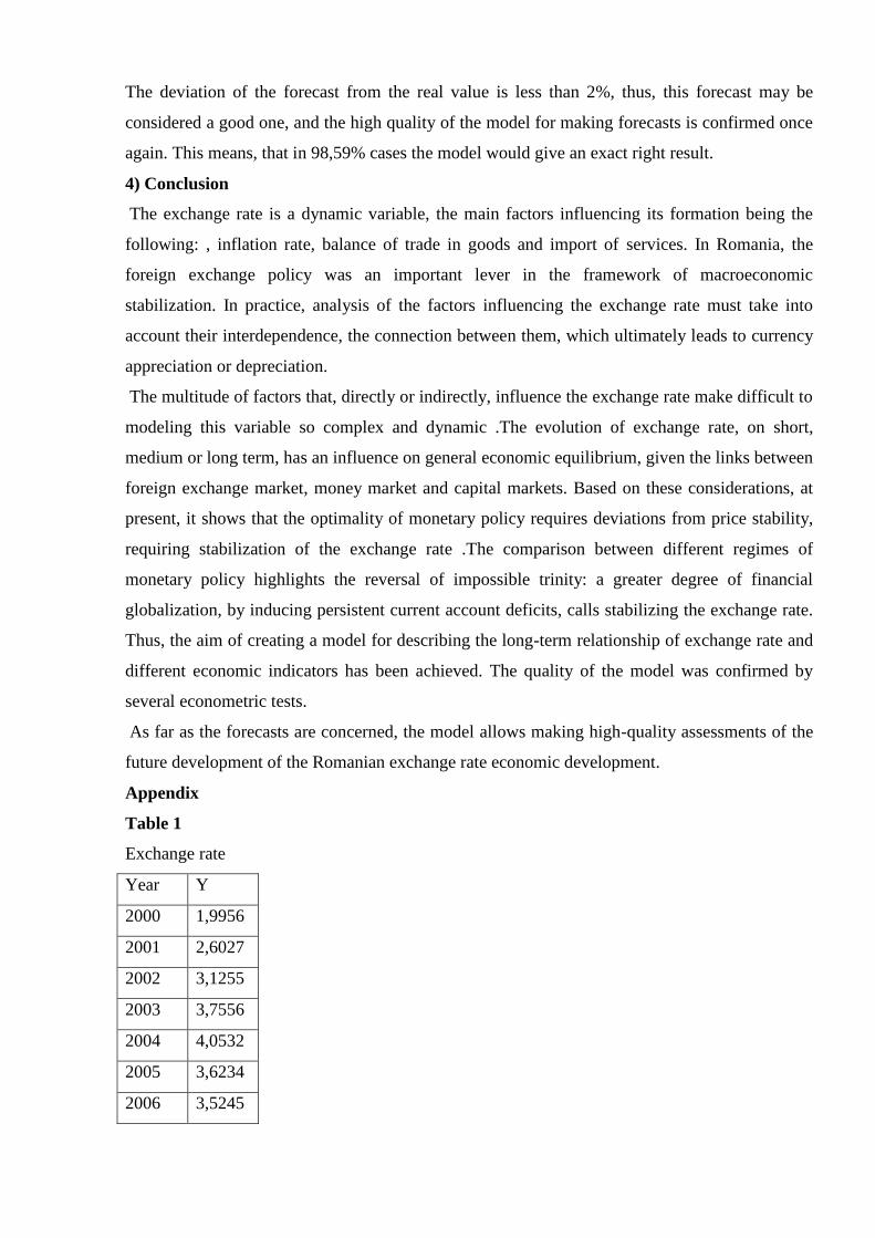
The evolution of exchange rate EUR/RON was not stable and linear, being marked by a
series of major fluctuations (see table 1 in appendix). Thus, since 2000 to 2004, EUR rose
continuously against RON with more than 100%, the trend began to reverse in time, the average
during the first nine months of 2008, being over 10 percent lower than the rate recorded in the
first days of 2004. The deterioration of confidence in the components of financial market,
following the financial crisis effects has putted pressure on the exchange rate. Since 2009 under
the impact of international crisis, domestic currency continued to depreciate more pronounced
against the euro. By the end of March 2009, the RON depreciated with 25% against the euro
from mid-2007 despite the increase of interest rates. The trend of depreciation of the exchange
rate was maintained during 2010.
Gross Domestic Product per capita at PPS (Purchasing Power Parity) EURO/Capita (X1)
In terms of GDP growth, the period 2000-2010 was one of the most glorious periods in
all history of the Romanian economy(see table 2 in appendix). During 2000-2006, GDP growth
was robust, being on average 7728, 5 (average calculated using initial table) per year. However,
at the end of 2007 the level of this indicator (expressed in purchasing power parity) stood for
Romania only at 10400 of the EU27 average. During 2007-2008 GDP increased massively due
to accession of our country to EU and due to strong growth of private capital inflows. Romanian
economy went into recession in the third quarter of 2008, when GDP decreased in 2009 from
12000 to 11000 in 2009. In 2010 the situation began to improve and in 2010 GDP began to
increase reached 11700 in 2011.
Inflation rate in % (X2)
Regarding inflation, Romania registered a positive trend during 2000- 2007(see table 3 in
appendix), because inflation rate gradually declined during that time. During 2000-2005,
Romania has experienced a strong disinflation, reaching single digits. After 2005 the inflationary
trend has registered slowing slightly. The lowest level of inflation was 4.9%, value recorded in
2007. In 2008 Romania ranked 5 in the European Union (EU), the indicator recorded, in our
country, a level of 6.4%, according to Eurostat. Average monthly inflation stood at 0.5%, as in
2007, while annual inflation average rose to 7.9%, three points above the 2007 level. The
inflation rate in 2010 stood 0.5 percentage points above the average of 2009, reaching 6.1%. The

increase occurred due to increasing the standard VAT rate by 5 percentage points, from 19% to
24%. And in 2011 annual average inflation rate decreased slightly and stood at 5, 8%.
Balance of Payment (X3)(Trade of goods only)
The trade policy in Romania has been characterized, in recent years, by restriction of the
possibilities to boost exports. Shares weak authorities, which sought to stimulate imports
(considerably cheaper) to have time for economic recovery, leaded to worsening external
imbalance. The trade balance recorded the largest deficits in 2007- 2008 given the expansion of
imports from the EU and exports decline.(see table 4 in appendix)
Interest rate in % (X4)
The interest rate practiced by the NBR (National Bank of Romania) in the period 2000-
2007 showed a downward trend(see table 5 in appendix), the most significant leap being
recorded in 2002 when it reached 27,3%. The reference interest is back on an upward trend in
2008 when its level was 12,3%, then continued downward trend in coming years. The financial
crisis has brought to the fore the importance of the interest rate in economic recovery process.
Under these conditions, the National Bank of Romania dropped the reference interest rate to
historic levels in order to stimulate economic growth.
3) Econometric model
After analyzing these economic indicators, Initial Table was constructed
Year Y X1 X2 X3 X4
2000 1,9956 6,5 45,7 -1,867 50,7
2001 2,6027 7 34,5 -3,323 41,3
2002 3,1255 7,4 22,5 -2,752 27,3
2003 3,7556 7,6 15,3 -3,955 17,1
2004 4,0532 7,9 11,9 -5,323 19,1
2005 3,6234 8,6 9,1 -7,806 8,4
2006 3,5245 9,1 6,6 -11,659 8,1
2007 3,3373 10,4 4,9 -17,822 7,2
2008 3,6827 12 7,9 -19,109 12,3
2009 4,2373 11 5,6 -6,871 11,3
2010 4,2099 11,2 6,1 -5,864 6,5
2011 4,2379 11,7 5,8 -5,549 6,25
Mathematically, the model should be as following:
Y=Exchange rate (ROL/EUR)
X1=Gross Domestic Product per capita at PPS (Purchasing Power Parity) EURO/Capita (divided
by 1000)
X2=Inflation rate ( in %)
X3=Trade Balance (in billions Euros)
X4=Interest rate ( in %)
{
a0...a4 </>0
where,
E is expectation of residual/disturbance term. Residual is, basically a difference between real and
theoretical points.
Et – is a disturbance term, showing random factors which can occur at any point in time and still
influence the endogenous variable.
σ - is a standard deviation
Identification of dependency between exchange rate(Y) and external factors influencing on
it (X1,…X4)
In order to find dependency between Y and X1,X2,X3,X4 we can construct matrix of pair
correlations and scatter diagrams.
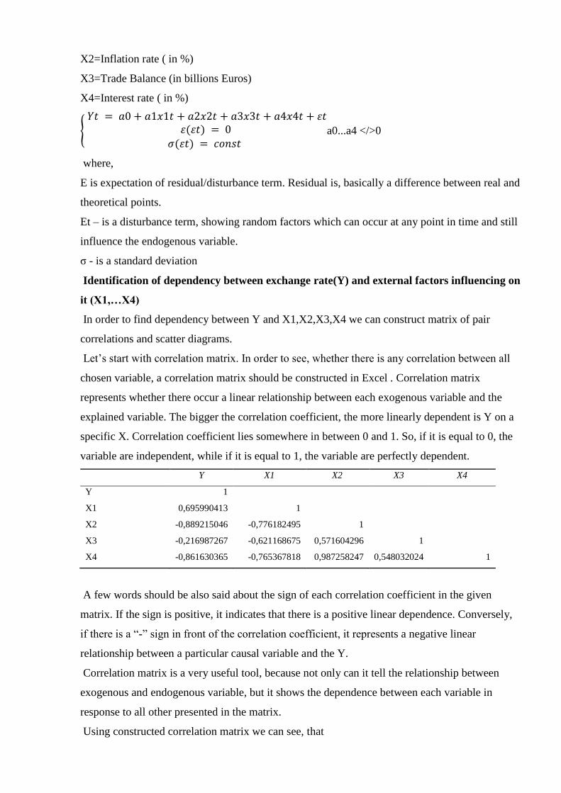
Let’s start with correlation matrix. In order to see, whether there is any correlation between all
chosen variable, a correlation matrix should be constructed in Excel . Correlation matrix
represents whether there occur a linear relationship between each exogenous variable and the
explained variable. The bigger the correlation coefficient, the more linearly dependent is Y on a
specific X. Correlation coefficient lies somewhere in between 0 and 1. So, if it is equal to 0, the
variable are independent, while if it is equal to 1, the variable are perfectly dependent.
Y X1 X2 X3 X4
Y 1
X1 0,695990413 1
X2 -0,889215046 -0,776182495 1
X3 -0,216987267 -0,621168675 0,571604296 1
X4 -0,861630365 -0,765367818 0,987258247 0,548032024 1
A few words should be also said about the sign of each correlation coefficient in the given
matrix. If the sign is positive, it indicates that there is a positive linear dependence. Conversely,
if there is a “-” sign in front of the correlation coefficient, it represents a negative linear
relationship between a particular causal variable and the Y.
Correlation matrix is a very useful tool, because not only can it tell the relationship between
exogenous and endogenous variable, but it shows the dependence between each variable in
response to all other presented in the matrix.
Using constructed correlation matrix we can see, that
If X1=0, 695990413 it has nearly strong positive linear relationship between X1 and Y;
If X2=0, 889215046 ~ 1 it has strong positive linear relationship between X2 and Y;
If X3=0, 216987267 it has weak positive linear relationship between X3 and Y;
If X4=0, 861630365 ~ 1 it has strong positive relationship between X4 and Y
Scatter diagrams
A scatter diagram is a tool for analyzing relationships between two variables. One variable is
plotted on the horizontal axis and the other is plotted on the vertical axis. The pattern of their
intersecting points can graphically show relationship patterns. Most often a scatter diagram is
used to prove or disprove cause-and-effect relationships. While the diagram shows relationships,
it does not by itself prove that one variable causes the other. In addition to showing possible
cause and- effect relationships, a scatter diagram can show that two variables are from a common
cause that is unknown or that one variable can be used as a surrogate for the other.
The dependence of the endogenous variable on each of the remaining exogenous variables was
investigated using scatter diagrams.
It is useful to create scatter diagrams to graphically show, how the statistics for each variable are
scattered through a trend line, representing the dependence of effect variable.
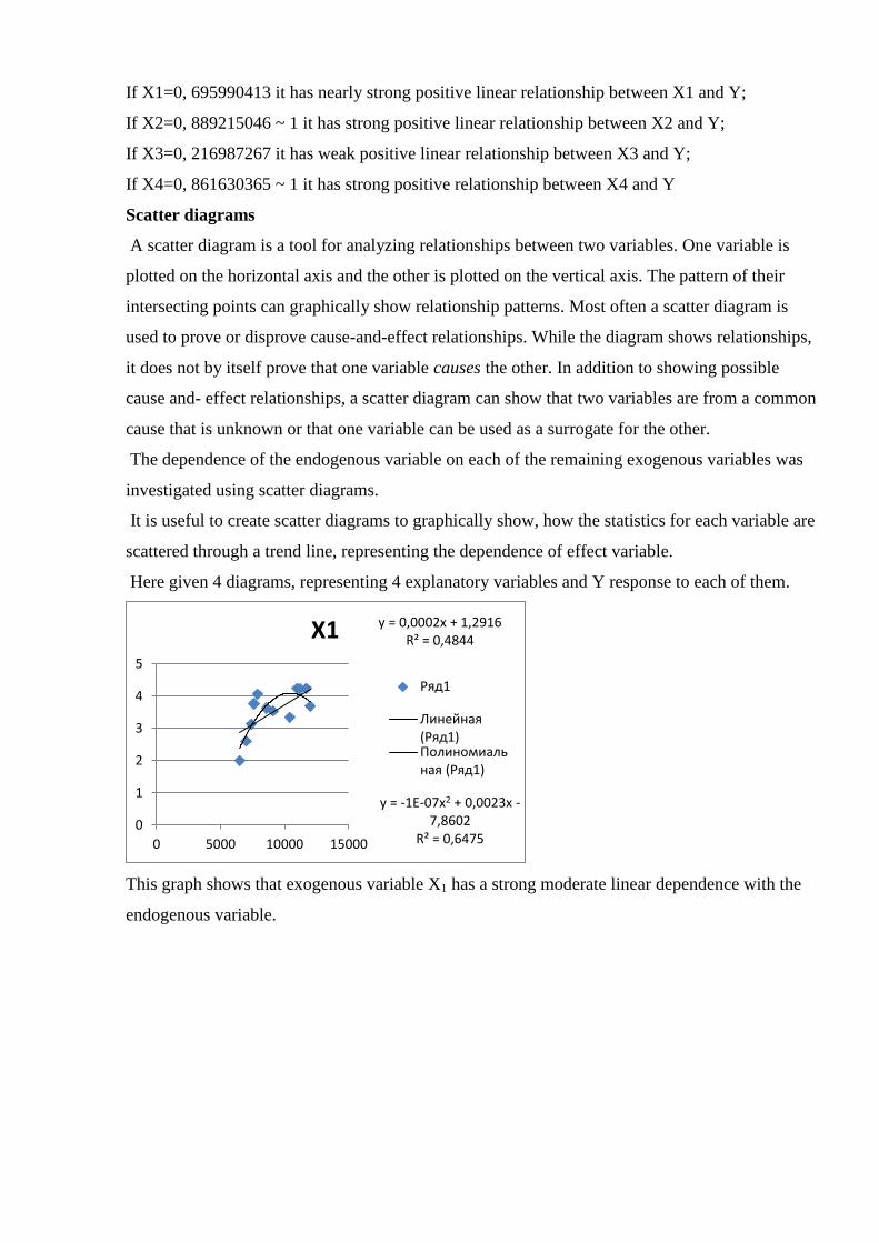
Here given 4 diagrams, representing 4 explanatory variables and Y response to each of them.
This graph shows that exogenous variable X1 has a strong moderate linear dependence with the
endogenous variable.
y = 0,0002x + 1,2916 R² = 0,4844
y = -1E-07x2 + 0,0023x - 7,8602
R² = 0,6475 0
1
2
3
4
5
0 5000 10000 15000
X1
Ряд1
Линейная (Ряд1) Полиномиальная (Ряд1)

This graph shows that exogenous variable X2 has a strong negative linear dependence with the
endogenous variable.
This graph shows that exogenous variable X3 has a moderate negative linear dependence with
the endogenous variable.
This graph shows that exogenous variable X4 has a strong negative linear dependence with the
endogenous variable.
General form of econometric model
General form of econometric model looks like
y = -0,0467x + 4,2168 R² = 0,7907
y = 4,3509e-0,016x R² = 0,8386 0
1
2
3
4
5
0 20 40 60
X2
Ряд1
Линейная (Ряд1) Экспоненциальная (Ряд1)
y = -3E-05x + 3,3301 R² = 0,0471
0
1
2
3
4
5
-30000 -20000 -10000 0
X3
Ряд1
Логарифмическая (Ряд1)
Линейная (Ряд1)
y = -0,0406x + 4,2618 R² = 0,7424
y = -0,0009x2 + 0,0067x + 3,8686
R² = 0,789 0
1
2
3
4
5
0 20 40 60
X4
Ряд1
Линейная (Ряд1) Полиномиальная (Ряд1)

{
a0...a4 </>0
where,
E is expectation of residual/disturbance term. Residual is, basically a difference between real and
theoretical points.
Et – is a disturbance term, showing random factors which can occur at any point in time and still
influence the endogenous variable.
σ - is a standard deviation
Estimated econometric model
{
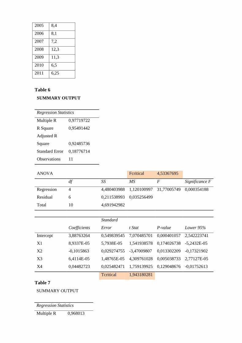
The value of adjusted R2 is 0.92. In other words, the model correctly explains 92% of all
observations. Adjusted R2 is close to 1, so R-test confirmed good quality of the model.
In order to confirm the significance of the model, we should check it by F-test(see table 6 in
appendix)
Using formula FРАСПОБР, F critical=4, 53367695
As F calculated > F critical (31, 77005749 > 4, 53367695), it means that is not randomly
chosen, so we have good quality of specification)
In order to find significance of the coefficients, we should check it by T-test(see table 6 in
appendix)
Using formula СТЬЮДРАСПОБР, T critical=1, 943180281
If absolute value of T statistical is higher than T critical, these coefficients are significant (
| |>Tcrit)
In model case,
is significant, because 7,070485701 > 1, 943180281
is not significant because 1,541938578 < 1, 943180281
is significant, because absolute value of -3,47009807 > 1, 943180281
is significant, because 4,309761028 > 1, 943180281
is not significant, because 1,759139925 < 1, 943180281
So, coefficients and are not significant, it means that change in Y(exchange rate) don’t
effect on X1( Gross Domestic Product) and on X4 (Interest rate)
Model without X1

Then we need to create the second model without X1,
Year Y X1 X2 X3
2000 1,9956 45,7 -1,867 50,7
2001 2,6027 34,5 -3,323 41,3
2002 3,1255 22,5 -2,752 27,3
2003 3,7556 15,3 -3,955 17,1
2004 4,0532 11,9 -5,323 19,1
2005 3,6234 9,1 -7,806 8,4
2006 3,5245 6,6 -11,659 8,1
2007 3,3373 4,9 -17,822 7,2
2008 3,6827 7,9 -19,109 12,3
2009 4,2373 5,6 -6,871 11,3
2010 4,2099 6,1 -5,864 6,5
2011 4,2379 5,8 -5,549 6,25
where
Y=Exchange rate (ROL/EUR)
X1=Inflation rate ( in %)
X2=Trade Balance (in billions Euros)
X3=Interest rate ( in %)
As in previous case we have made regression analyses and made F-test and T-test
In this case coefficients , , are significant, because ( | |>Tcrit) , but coefficient
is not significant, , it means that change in Y(exchange rate) don’t effect on X3( Interest rate)
(see table 7 in appendix)
I order not to remove this coefficient, we have tried to change time period and use and
again made regression analyses, F-test and T-test
But this technique hasn’t changed anything, so we have decided to remove this variable and find
new one, that will be significant for my model.
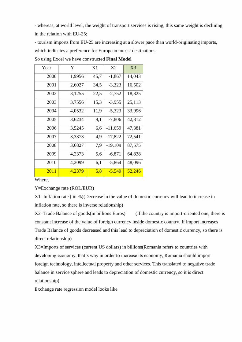
Final Model
Model with new variable
From the Trade balance of Romania, we can see that number of imports always higher than
number of exports, it means that Romania is import-oriented country.
And we want to introduce a new variable X3- Imports of services (current US$) in millions.
From the analysis of the structure of Romania’s services imports, we can note the following:
- their sectorial distribution is similar at both levels: world and European;
- whereas, at world level, the weight of transport services is rising, this same weight is declining
in the relation with EU-25;
- tourism imports from EU-25 are increasing at a slower pace than world-originating imports,
which indicates a preference for European tourist destinations.
So using Excel we have constructed Final Model
Year Y X1 X2 X3
2000 1,9956 45,7 -1,867 14,043
2001 2,6027 34,5 -3,323 16,502
2002 3,1255 22,5 -2,752 18,825
2003 3,7556 15,3 -3,955 25,113
2004 4,0532 11,9 -5,323 33,996
2005 3,6234 9,1 -7,806 42,812
2006 3,5245 6,6 -11,659 47,381
2007 3,3373 4,9 -17,822 72,541
2008 3,6827 7,9 -19,109 87,575
2009 4,2373 5,6 -6,871 64,838
2010 4,2099 6,1 -5,864 48,096
2011 4,2379 5,8 -5,549 52,246
Where,
Y=Exchange rate (ROL/EUR)
X1=Inflation rate ( in %)(Decrease in the value of domestic currency will lead to increase in
inflation rate, so there is inverse relationship)
X2=Trade Balance of goods(in billions Euros) (If the country is import-oriented one, there is
constant increase of the value of foreign currency inside domestic country. If import increases
Trade Balance of goods decreased and this lead to depreciation of domestic currency, so there is
direct relationship)
X3=Imports of services (current US dollars) in billions(Romania refers to countries with
developing economy, that’s why in order to increase its economy, Romania should import
foreign technology, intellectual property and other services. This translated to negative trade
balance in service sphere and leads to depreciation of domestic currency, so it is direct
relationship)
Exchange rate regression model looks like

Tests: R²-Test, F-Test, T-Test, GQ-Test, DW-Test,R-test
We can see that as F calculated > F critical (36, 42436 > 4, 346831), it means that is not
randomly chosen, so we have good quality of specification)
is close to one, it means that Var(X1) describes Var(X2) by approximately 91%.
And as ( | |>Tcrit) in all four cases is right, it means that all coefficients are significant in
this model.(see table 8 in appendix)
Let’s carry out Goldfeld-Quandt test to check the estimated model for homoscedasticity. To do
the test, a new variable z was introduced, such that:
Then dataset was sorted (in descending order) according to the values of z. After the sorting,
residual sum of squares (RSS) was found separately for two samples, consisting of upper and
lower observations (the results of these calculations are given in table 9 in appendix). Based on
these numbers, let’s find the GQ number by dividing the bigger RSS by the smaller one.
To complete the test, the GQ number has to be compared with the critical value of F-statistic,
which equals 9,27 at 5% level of significance. The GQ number calculated above is less than the
critical value of F-statistic.
Thus, the hypothesis of homoscedasticity of residuals in the final estimated model is confirmed
at 10% level of significance, according to GQ-test. So, GQ-test is passed successfully – the
model can be estimated through least square method.
Let’s carry out Durbin-Watson test to check the residuals of the model for autocorrelation. To
do the test, estimated values of Y were calculated for each year, using the coefficients obtained
in regression analysis .Then, the residual value for each year was found as the difference
between actual and estimated values of Y. Finally, for each year except the first one, the
difference between the residual for current and previous year was calculated.(see table 10 in
appendix)
On the basis of these calculations, the following results were obtained:
∑

∑
Thus, the value of the Durbin-Watson statistic for the final estimated model is:
∑
∑
The observed value of Durbin-Watson (calculated on the basis of sample data) is compared with
the critical value of Durbin-Watson, which is determined on a special table.
The critical value of Durbin-Watson is determined depending on the values of the upper and
lower d1 d2 border criterion on special tables. These boundaries are defined, depending on the
volume of sample n and the number of degrees of freedom (h-1), where h - number of evaluated
sample parameters.
If the observed value of the Durbin-Watson is less than the critical value of the lower boundary,
d <d1, then the fundamental hypothesis of no autocorrelation between the residuals of the
regression model is rejected.
If the observed value of the Durbin-Watson more critical of its upper boundary, d> d2, then the
fundamental hypothesis of no first order autocorrelation between the residuals of the regression
model is adopted.
If the observed value of the Durbin-Watson is between the upper and lower critical limits, that
is, d1 <d<d2, adequate justification for making no single solution, further research is needed.
If the observed value of the Durbin-Watson more critical level 4 - d1, d> 4 - d1, then the
fundamental hypothesis of no first order autocorrelation between the residuals of the regression
model is again rejected.
If the observed value of the Durbin-Watson is less than the critical value 4 - d2, d<4 - d2, then
the fundamental hypothesis of no first order autocorrelation between the residuals of the
regression model is once again adopted.
If the observed value of the Durbin-Watson is in the critical interval between the values of 4 - d1
and 4 - d2, is a sufficient basis for making the right decision is not only more research is needed.
This value was compared with upper and lower limits of DW-statistic
dl = 0,60
du = 1,93

4-dl = 3,4
4-du = 2,07
2,07< 2,49 < 3,4
Confidence intervals
In order to find out whether the estimated model is good for forecasting, let’s construct the
confidence interval and check whether the real value of Y in 2011 (the last observation), which
equals 4,23 belongs to this interval.
The lower and upper boundaries of the confidence interval are calculated by the following
formulas:
Where
Substituting real values of explanatory variables for 2011 and the coefficients of the estimated
model (see table…….) into this formula, get:
(see table 10 in appendix)
The value of s (standard error of the model) and critical value of t-statistic have been calculated
earlier in the regression statistics (see table …)
They are:
0,2
Thus, the boundaries of the confidence interval are:
One can easily check that 4, 30∈[3,92; 4,68]
It follows that the real value of Y in 2011 belongs to the confidence interval, so the model is
adequate and may be used for forecasting.
Forecasting
It has already been calculated that the model predicts the value of Y in 2011 to be equal to 4,30 ,
while its real value was 4,24. In order to find out whether this forecast is good, let’s calculate the
percentage deviation of the forecast from the real value.
| |
The deviation of the forecast from the real value is less than 2%, thus, this forecast may be
considered a good one, and the high quality of the model for making forecasts is confirmed once
again. This means, that in 98,59% cases the model would give an exact right result.
4) Conclusion
The exchange rate is a dynamic variable, the main factors influencing its formation being the
following: , inflation rate, balance of trade in goods and import of services. In Romania, the
foreign exchange policy was an important lever in the framework of macroeconomic
stabilization. In practice, analysis of the factors influencing the exchange rate must take into
account their interdependence, the connection between them, which ultimately leads to currency
appreciation or depreciation.
The multitude of factors that, directly or indirectly, influence the exchange rate make difficult to
modeling this variable so complex and dynamic .The evolution of exchange rate, on short,
medium or long term, has an influence on general economic equilibrium, given the links between
foreign exchange market, money market and capital markets. Based on these considerations, at
present, it shows that the optimality of monetary policy requires deviations from price stability,
requiring stabilization of the exchange rate .The comparison between different regimes of
monetary policy highlights the reversal of impossible trinity: a greater degree of financial
globalization, by inducing persistent current account deficits, calls stabilizing the exchange rate.
Thus, the aim of creating a model for describing the long-term relationship of exchange rate and
different economic indicators has been achieved. The quality of the model was confirmed by
several econometric tests.
As far as the forecasts are concerned, the model allows making high-quality assessments of the
future development of the Romanian exchange rate economic development.
Appendix
Table 1
Exchange rate
Year Y
2000 1,9956
2001 2,6027
2002 3,1255
2003 3,7556
2004 4,0532
2005 3,6234
2006 3,5245

2007 3,3373
2008 3,6827
2009 4,2373
2010 4,2099
2011 4,2379
Table 2
Gross Domestic Product per capita at PPS (Purchasing Power Parity) EURO/Capita (X1)
Year 2000 2001 2002 2003 2004 2005 2006 2007 2008 2009 2010 2011
GDP 6500 7000 7400 7600 7900 8600 9100 10400 12000 11000 11200 11700
Table 3
Inflation rate in %
Year 2000 2001 2002 2003 2004 2005 2006 2007 2008 2009 2010 2011
Annual
average
inflation
rates
45,7 34,5 22,5 15,3 11,9 9,1 6,6 4,9 7,9 5.6 6.1 5.8
Table 4
Balance of Payment (X3)(Trade of goods only)
Year 2000 2001 2002 2003 2004 2005 2006 2007 2008 2009 2010 2011
Export 11273 12722 14675 15614 18935 22255 25850 29549 33725 29084 37251 41237
Import 13140 16045 17427 19569 24258 30061 37509 47371 52834 35955 43115 46786
Trade
balance
-1867 -3323 -2752 -3955 -5323 -7806 -
11659
-
17822
-
19109
-6871 -5864 -5549
All numbers are given in millions Euro
Table 5
Interest rate in %
Year Interest rate
2000 50,7
2001 41,3
2002 27,3
2003 17,1
2004 19,1
2005 8,4
2006 8,1
2007 7,2
2008 12,3
2009 11,3
2010 6,5
2011 6,25
Table 6
SUMMARY OUTPUT
Regression Statistics
Multiple R 0,97719722
R Square 0,95491442
Adjusted R
Square 0,92485736
Standard Error 0,18776714
Observations 11
ANOVA
Fcritical 4,53367695
df SS MS F Significance F
Regression 4 4,480403988 1,120100997 31,77005749 0,000354188
Residual 6 0,211538993 0,035256499
Total 10 4,691942982
Coefficients
Standard
Error t Stat P-value Lower 95%
Intercept 3,88763264 0,549839545 7,070485701 0,000401057 2,542223741
X1 8,9337E-05 5,7938E-05 1,541938578 0,174026738 -5,2432E-05
X2 -0,1015863 0,029274755 -3,47009807 0,013302209 -0,17321902
X3 6,4114E-05 1,48765E-05 4,309761028 0,005038733 2,77127E-05
X4 0,04482723 0,025482471 1,759139925 0,129048676 -0,01752613
Tcritical 1,943180281
Table 7
SUMMARY OUTPUT
Regression Statistics
Multiple R 0,968013

R Square 0,937049
Adjusted R
Square 0,91007
Standard Error 0,205414
Observations 11
ANOVA
Fcritical 4,346831
df SS MS F
Significance
F
Regression 3 4,396579 1,465526 34,73235 0,000142
Residual 7 0,295364 0,042195
Total 10 4,691943
Coefficients
Standard
Error t Stat P-value Lower 95%
Intercept 4,686962 0,200508 23,37548 6,66E-08 4,212837
X1 -0,11323 0,030943 -3,65917 0,008079 -0,18639
X2 5,23E-05 1,39E-05 3,749496 0,007173 1,93E-05
X3 0,049528 0,027677 1,789472 0,116668 -0,01592
Tcritical 1,894579
Table 8
SUMMARY OUTPUT
Regression Statistics
Multiple R 0,969431227
R Square 0,939796905
Adjusted R
Square 0,913995578
Standard Error 0,200880025
Observations 11
ANOVA
Fcritical 4,346831
df SS MS F
Significance
F
Regression 3 4,40947 1,469824 36,42436 0,000121694
Residual 7 0,28247 0,040353
Total 10 4,69194

Coefficients
Standard
Error t Stat P-value Lower 95%
Intercept 4,370053073 0,28599 15,28017 1,24E-06 3,693782393
X1 -0,050770019 0,00735 -6,9073 0,00023 -0,06815046
X2 0,091313467 0,02503 3,648443 0,008195 0,032131495
X3 0,013987276 0,0073 1,915184 0,097015 -0,00328242
Tcritical 1,894579
Table 9
Year Y X1 X2 X3 Z
2000 1,9956 45,7 -1867 14043 15955,7
2001 2,6027 34,5 -3323 16502 19859,5
2002 3,1255 22,5 -2752 18825 21599,5
2003 3,7556 15,3 -3955 25113 29083,3
2004 4,0532 11,9 -5323 33996 39330,9
2005 3,6234 9,1 -7806 42812 50627,1
2006 3,5245 6,6 -11659 47381 59046,6
2007 3,3373 4,9 -17822 72541 90367,9
2008 3,6827 7,9 -19109 87575 106691,9
2009 4,2373 5,6 -6871 64838 71714,6
2010 4,2099 6,1 -5864 48096 53966,1
2011 4,2379 5,8 -5549 52246 57800,8
GQ test
GQ 1,095087
1/GQ 0,913169
Table 10
RESIDUAL OUTPUT
Observation Predicted Y Residuals ei-1 (ei-ei-1)^2 ei^2
1 2,075804277 -0,0802
2 2,545870792 0,05683 -0,0802 0,018778 0,003229559
3 3,239743449 -0,11424 0,056829 0,029266 0,013051566
4 3,583389473 0,17221 -0,11424 0,082056 0,029656466
5 3,755339683 0,29786 0,172211 0,015788 0,088720768
6 3,794076219 -0,17068 0,29786 0,219526 0,029130372

7 3,63307834 -0,10858 -0,17068 0,003856 0,011789256
8 3,508542328 -0,17124 -0,10858 0,003927 0,029323935
9 3,44899654 0,2337 -0,17124 0,163981 0,054617307
10 4,365233107 -0,12793 0,233703 0,130781 0,01636688
11 4,197625792 0,01227 -0,12793 0,019658 0,000150656
Theoretical 4,299667733
0,012274
Y+ 4,68025073
CYMM 0,687617 0,276036764
Y- 3,919084736
DW 2,491035