WP/07/261

Effect of IMF Structural Adjustment Programs on Expectations: The Case of

Transition Economies

Patrick Imam

© 2007 International Monetary Fund WP/07/261 IMF Working Paper African Department Effect of IMF Structural Adjustment Programs on Expectations: The Case of Transition

Economies1

Prepared by Patrick Imam

Authorized for distribution by Arend Kouwenaar November 2007

Abstract

This Working Paper should not be reported as representing the views of the IMF. The views expressed in this Working Paper are those of the author(s) and do not necessarily represent those of the IMF or IMF policy. Working Papers describe research in progress by the author(s) and are published to elicit comments and to further debate.

We analyze the effect of IMF programs on economic agents’ expectations about the economy in transitional countries using survey data from the Central and Eastern Eurobarometer poll, an annual general public survey monitoring the evolution of public opinion from 1990 to 1997. Previous studies, in contrast, have looked at indirect measures, such as capital flows or yield spreads, to assess the impact of IMF programs on economic expectations. Using a multinomial probit model, we find that IMF loans appear to have a strong effect on agent expectations in the early years, through the inflow of real money, and through the signaling effect. IMF programs during periods of collapsing growth appear to reinforce underlying expectations for the future; they are associated with positive expectations for those with an optimistic outlook and negative expectations for those with a negative outlook. Once recovery is underway, and economic uncertainty diminishes, it appears that IMF programs cease to have a statistically significant effect on the expectations of economic agents. This suggests that IMF programs have the biggest impact on expectations during periods of great uncertainty and less of an impact when countries are subject to minor shocks. JEL Classification Numbers:

Keywords: Structural Adjustment, Transition Economies Author’s E-Mail Address: pimam@imf.org 1 I would like to thank seminar participants at the IMF Institute seminar. Special thanks are also due to Ales Bulir, Burkhard Drees, Jemma Dridi, Maher Hassan, Elizabeth Miranda and Juan Zalduendo. The usual disclaimer applies.

2

Contents Page

I. Introduction ............................................................................................................................3

II. Conceptual Issues in Measuring ‘Expectations’ ...................................................................5 A. How Do Economists Model Expectations? ..............................................................5

Background........................................................................................................5 Adaptive Expectations .......................................................................................6 Rational Expectations ........................................................................................7 Bounded Rationality ..........................................................................................8

B. Measurement of Expectations ...................................................................................8 C. Advantage of Using Survey Data............................................................................10

III. Econometric Estimation.....................................................................................................11 A. Data .........................................................................................................................11 B. Econometric Analysis .............................................................................................14 C. Main Results............................................................................................................17

Effect of Personal Characteristics on Expectations .........................................19 Effect of Macro-Variables on Expectations.....................................................20 Effect of IMF Programs on Expectations ........................................................22 Robustness Test: Comparing 1990-93 with 1994-97 ......................................23

IV. Conclusion .........................................................................................................................26

V. Reference ............................................................................................................................27

Appendix 1...............................................................................................................................30

3

I. INTRODUCTION

One of the key functions of the IMF is to restore investor and consumer confidence in countries facing macroeconomic imbalances, primarily through structural adjustment programs (IEO, 2002)2 This is reflected in Article I of the Articles of Agreement, which states that the IMF’s role is to

“give confidence to members by making the general resources of the Fund temporarily available to them under adequate safeguards, thus providing them with opportunity to correct maladjustments in their balance of payments without resorting to measures destructive of national or international prosperity” [emphasis added].

The rationale is that a temporary IMF program should give countries facing macroeconomic imbalances breathing space so they can achieve a smooth adjustment without resorting to drastic actions that could harm long-term growth prospects (e.g., indiscriminate capital spending cuts). If an IMF program restores the public’s confidence in the future health of an economy, the thinking goes, then consumers spending and investment will resume, which should help revive growth.

IMF structural programs, however, have been widely criticized for failing to restore economic growth and confidence. A much-cited paper by Barro and Lee (2005) based on a panel of all 725 IMF loans between 1970 and 2000 concludes that “the typical country would be better off economically if it committed itself not to be involved with IMF loan programs” (p.1). Radelet and Sachs (1998) similarly assert that IMF programs do not improve expectations about the health of the economy. They claim that IMF programs are

“... far from optimal for restoring financial market confidence in the short term....” [emphasis added].

Other studies, however, arrive at a more positive conclusion (see, for example, Mody and Rebucci, 2006).

“bailout granted conditional on policy adjustment by the debtor country can restore investors’ confidence and voluntary lending and therefore stop destructive runs — i.e., can have a ‘catalytic effect’.” (p.2) [emphasis added]

These divergent views on the effect of IMF programs on expectations in part reflect the different (and often imperfect) methodologies used. Most empirical work on the effect of IMF programs has not used data on expectations (which are hard to measure) but has instead looked at how the economy performed against selected benchmarks after IMF programs. The implicit justification behind the use of this methodology—as opposed to one that measures expectations directly—is that a country’s economy will only do better after an IMF program 2 In this paper, “confidence” in the future and “expectations” are used interchangeably. If an individual has positive confidence in the future, he or she has a positive forecast of the economy and vice versa.

4

if such a program improves public expectations. Otherwise, economic agents will refrain from consuming and investing, and growth will stall. In other words, improved economic growth goes hand-in-hand with improved economic expectations. A problem is that past studies that assessed the impact of IMF programs on restoring economic health have fundamental methodological weaknesses, making it difficult to establish strong conclusions (see Ul Haque and Khan, 1998, for a summary of such weaknesses).

The first methodology used was the before-after approach, which compares macroeconomic variables before and after a program was implemented. The idea of measuring the counterfactual is problematic, however; the before-after approach unrealistically assumes that all else is equal.

A second method is the with-without approach; this method compares the macroeconomic performance of countries with programs to those without programs. This approach assumes that countries requiring IMF programs are similar to countries that do not require them—a problematic assumption, especially because selection bias may be involved in determining which countries require IMF programs (see Goldstein and Montiel, 1986).

Third, the generalized evaluation approach aims to compare countries with a program and those without a program by adjusting for exogenous influences, such as different growth rates. The generalized evaluation approach requires researchers to gather information on many exogenous variables that are difficult to quantify or approximate (e.g., policy reaction functions), making it hard to arrive at robust conclusions (Khan, 1990).

Finally, the simulations approach compares the situation under an IMF program to that under a simulated counterfactual without an IMF program. The model used under this approach covers a range of policy measures used in IMF programs, and requires assumptions that cannot be tested in practice to be formulated (Khan et al., 1991).

Besides these methodological weaknesses, the economic literature has paid scant attention to the effect of IMF programs on expectations, largely because expectations are hard to measure. The few studies trying to measure how IMF programs affect consumers’ and investors’ expectations have used proxies, such as capital flows (see Goldstein, 2000, for a summary of the arguments). Given that most studies that use capital inflows by foreigners and repatriations by domestic investors as a proxy to measure investors’ expectations about the future of the economy did not find a resumptions in inflows, critics point out to a failure of IMF programs in restoring confidence in the economy (see e.g. Radelet and Sachs, 1998, and Furman and Stiglitz, 1998). Such studies, however, overlook the fact that capital flows are not exclusively driven by expectations. For example, herding behavior can affect capital flows, but is often a sign of imperfect/lack of information or panic rather than poor expectations of future economic performance.

This paper assesses the effect of IMF programs on confidence using survey data measuring people’s expectations about the health of the economy following IMF programs. This is the first paper, to our knowledge, that empirically assesses how domestic agents incorporate IMF programs in their future outlook of the economy. Relying on answers of economic agents from surveys (i.e., their stated preferences), as opposed to their actions (i.e., their revealed

5

preferences) can provide new information about how IMF programs actually affect the public’s forecast about the future. The use of subjective data is a departure from traditional economics, where individual’s preferences are in general inferred from individuals’ actions. Using survey data on transition economies from 1990-97, our results suggest that IMF programs do have a strong effect on agents’ expectations in the early years of a growth collapse (1990–93), through the inflow of real money, and through the signaling effect. IMF programs during periods of collapsing growth reinforce underlying expectations about the future; indeed, they are positive for those with an optimistic outlook but are negative for those with a negative outlook. Once the growth collapse ends (1994–97), and with economic uncertainty diminished, IMF programs cease to have a statistically significant effect on the expectation of economic agents, regardless of their overall outlook for the economy. This implies that IMF programs are crucial during economic collapses in formerly communist countries but are less influential once countries have successfully transitioned toward capitalism.

It is not our intention to debate the impact of IMF structural programs on macroeconomic variables directly but rather to assess their impact on public expectations about the future of the economy, as measured by survey data. The paper should therefore not be seen as an assessment of whether IMF programs “succeed” or “fail,” as it does not try to assess the effect of IMF programs on economic imbalances. At best, this paper tests indirectly the effect of the success or failure of IMF programs by analyzing how it has actually affected economic agents’ confidence in the economy. Therefore, this study should be seen as a complement to, rather than a substitute for, previous studies looking at real economic outcomes of IMF programs.

The paper is structured as follows. In Part 2, we look at the problem of how to conceptually measure “expectations.” After showing the advantages of survey data of expectations over proxies such as capital flows, we proceed to examine how IMF programs affected expectations in transition economies. We test our hypothesis using a multinomial-ordered probit model. We then analyze our results and conclude.

II. CONCEPTUAL ISSUES IN MEASURING ‘EXPECTATIONS’

A. How Do Economists Model Expectations?

Background Expectation, defined as “to look forward” (see Merriam-Webster’s), is a fundamental concept in macroeconomics. Economic decision making is essentially based on expectations, as the action of economic agents are determined by what they think will happen in the future. Expectations are, however, (subjective) beliefs held by individuals about future outcomes, since by definition, the future is not known and expectations are therefore based on uncertainty. Because of this difficulty, formalizing the process of expectation formation has taken economists a long time.

6

Economists initially adopted ad hoc assumptions about the process of expectation formation. The problem with ad hoc measures is that they are inherently arbitrary. It was only with Knight (1921) that the first attempts were made to develop models of expectations. Knight made a distinction between “risk” and “uncertainty.” While in the case of the former, an individual does not know with certainty which outcome will arise, he or she can attach certain probabilities to outcomes. In the case of uncertainty, individuals cannot attach a probability. In this framework, it is therefore possible to forecast risk objectively, but it is not possible to forecast uncertainty.

Savage (1954), however, criticized the distinction between risk and uncertainty. According to him, in real life, agents subject to uncertainty form expectations as if they held beliefs that were represented by a probability distribution. In other words, the formation of expectations under risk and uncertainty will be similar, making Knight’s classification redundant. Keynes was even more critical of Knight, arguing that economic agents are too ignorant to form reliable probability distributions. Many situations are too rare for individuals to be able to form statistical estimates of outcomes. Rather than forming expectations based on probability, individual’s expectations are driven by “animal spirits,” meaning that economic agents form expectations based on instinct, preferences, habits, etc. Keynes argued that if economic agents are under Knightian uncertainty, the lack of information would mean that economic agents would not be able to form expectations.3 While Keynes’s insights were helpful in showing the limits of probability theory, they were extreme, as they minimized the role of economic theory in explaining the formation of agent’s expectations.

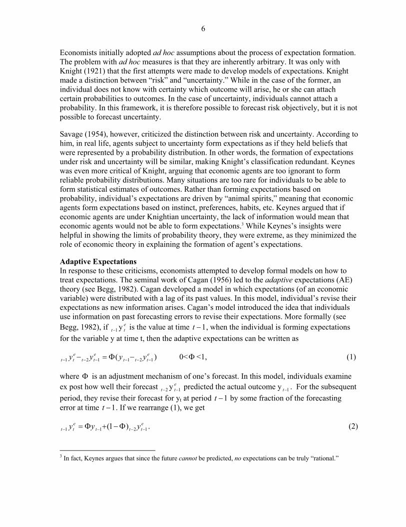
Adaptive Expectations In response to these criticisms, economists attempted to develop formal models on how to treat expectations. The seminal work of Cagan (1956) led to the adaptive expectations (AE) theory (see Begg, 1982). Cagan developed a model in which expectations (of an economic variable) were distributed with a lag of its past values. In this model, individual’s revise their expectations as new information arises. Cagan’s model introduced the idea that individuals use information on past forecasting errors to revise their expectations. More formally (see Begg, 1982), if 1−t y e

t is the value at time 1−t , when the individual is forming expectations for the variable y at time t, then the adaptive expectations can be written as

ettt

ett

ett yyyy 121121 ( −−−−−− −Φ=− ) 0<Φ <1, (1)

where Φ is an adjustment mechanism of one’s forecast. In this model, individuals examine ex post how well their forecast 2−t y e

t 1− predicted the actual outcome y 1−t . For the subsequent period, they revise their forecast for yt at period 1−t by some fraction of the forecasting error at time 1−t . If we rearrange (1), we get

ettt

ett yyy 1211 )1( −−−− Φ−+Φ= . (2)

3 In fact, Keynes argues that since the future cannot be predicted, no expectations can be truly “rational.”

7

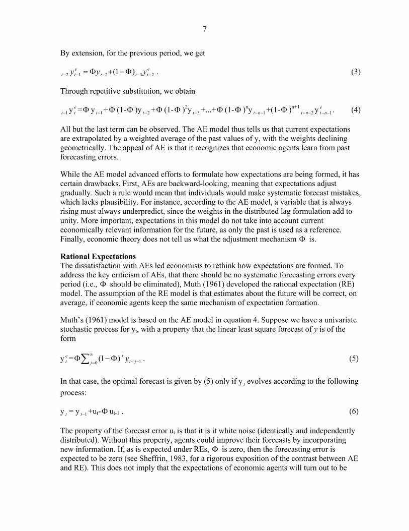
By extension, for the previous period, we get

ettt

ett yyy 23212 )1( −−−−− Φ−+Φ= . (3)

Through repetitive substitution, we obtain

1−t y et =Φ y 1−t +Φ (1-Φ )y 2−t +Φ (1-Φ )2y 3−t +...+Φ (1-Φ )ny 1−−nt +(1-Φ )n+1

2−−nt y ent 1−− . (4)

All but the last term can be observed. The AE model thus tells us that current expectations are extrapolated by a weighted average of the past values of y, with the weights declining geometrically. The appeal of AE is that it recognizes that economic agents learn from past forecasting errors.

While the AE model advanced efforts to formulate how expectations are being formed, it has certain drawbacks. First, AEs are backward-looking, meaning that expectations adjust gradually. Such a rule would mean that individuals would make systematic forecast mistakes, which lacks plausibility. For instance, according to the AE model, a variable that is always rising must always underpredict, since the weights in the distributed lag formulation add to unity. More important, expectations in this model do not take into account current economically relevant information for the future, as only the past is used as a reference. Finally, economic theory does not tell us what the adjustment mechanism Φ is.

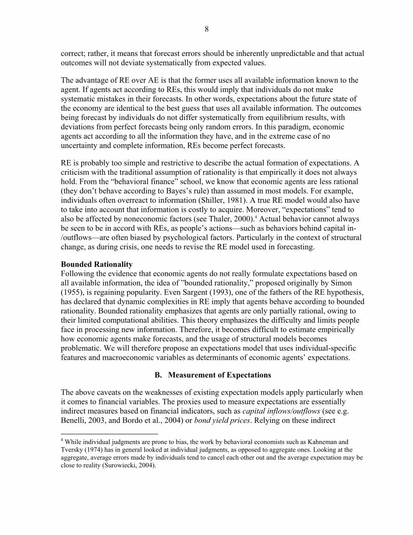
Rational Expectations The dissatisfaction with AEs led economists to rethink how expectations are formed. To address the key criticism of AEs, that there should be no systematic forecasting errors every period (i.e., Φ should be eliminated), Muth (1961) developed the rational expectation (RE) model. The assumption of the RE model is that estimates about the future will be correct, on average, if economic agents keep the same mechanism of expectation formation.

Muth’s (1961) model is based on the AE model in equation 4. Suppose we have a univariate stochastic process for yt, with a property that the linear least square forecast of y is of the form

y et = ∑∞

= −−Φ−Φ0 1)1(

j jtj y . (5)

In that case, the optimal forecast is given by (5) only if y t evolves according to the following process:

y t = y 1−t +ut-Φ ut-1 . (6)

The property of the forecast error ut is that it is it white noise (identically and independently distributed). Without this property, agents could improve their forecasts by incorporating new information. If, as is expected under REs, Φ is zero, then the forecasting error is expected to be zero (see Sheffrin, 1983, for a rigorous exposition of the contrast between AE and RE). This does not imply that the expectations of economic agents will turn out to be

8

correct; rather, it means that forecast errors should be inherently unpredictable and that actual outcomes will not deviate systematically from expected values.

The advantage of RE over AE is that the former uses all available information known to the agent. If agents act according to REs, this would imply that individuals do not make systematic mistakes in their forecasts. In other words, expectations about the future state of the economy are identical to the best guess that uses all available information. The outcomes being forecast by individuals do not differ systematically from equilibrium results, with deviations from perfect forecasts being only random errors. In this paradigm, economic agents act according to all the information they have, and in the extreme case of no uncertainty and complete information, REs become perfect forecasts.

RE is probably too simple and restrictive to describe the actual formation of expectations. A criticism with the traditional assumption of rationality is that empirically it does not always hold. From the “behavioral finance” school, we know that economic agents are less rational (they don’t behave according to Bayes’s rule) than assumed in most models. For example, individuals often overreact to information (Shiller, 1981). A true RE model would also have to take into account that information is costly to acquire. Moreover, “expectations” tend to also be affected by noneconomic factors (see Thaler, 2000).4 Actual behavior cannot always be seen to be in accord with REs, as people’s actions—such as behaviors behind capital in-/outflows—are often biased by psychological factors. Particularly in the context of structural change, as during crisis, one needs to revise the RE model used in forecasting.

Bounded Rationality Following the evidence that economic agents do not really formulate expectations based on all available information, the idea of ”bounded rationality,” proposed originally by Simon (1955), is regaining popularity. Even Sargent (1993), one of the fathers of the RE hypothesis, has declared that dynamic complexities in RE imply that agents behave according to bounded rationality. Bounded rationality emphasizes that agents are only partially rational, owing to their limited computational abilities. This theory emphasizes the difficulty and limits people face in processing new information. Therefore, it becomes difficult to estimate empirically how economic agents make forecasts, and the usage of structural models becomes problematic. We will therefore propose an expectations model that uses individual-specific features and macroeconomic variables as determinants of economic agents’ expectations.

B. Measurement of Expectations

The above caveats on the weaknesses of existing expectation models apply particularly when it comes to financial variables. The proxies used to measure expectations are essentially indirect measures based on financial indicators, such as capital inflows/outflows (see e.g. Benelli, 2003, and Bordo et al., 2004) or bond yield prices. Relying on these indirect 4 While individual judgments are prone to bias, the work by behavioral economists such as Kahneman and Tversky (1974) has in general looked at individual judgments, as opposed to aggregate ones. Looking at the aggregate, average errors made by individuals tend to cancel each other out and the average expectation may be close to reality (Surowiecki, 2004).

9

measures has in principle several advantages. Capital flows and bond yields are seen as an easy way to measure and quantify people’s expectations. Therefore, people’s actions are seen as good approximations of economic agents’ expectations, as actions speak louder than words.

A problem with using financial variables as a proxy for expectations is that this implicitly assumes that markets (and financial actors) are efficient and driven by fundamentals.5 Particularly in times of financial distress, when IMF programs take place, this does not necessarily hold, as will be illustrated below. Therefore, if capital does not flow back into a country after an IMF program, this might not be the result of the program not improving the expectations of economic agents, but of other factors.

First, during times of uncertainty, investors’ actions are not necessarily driven by their confidence in the fundamentals of the local economy but by how they see other investors react.6 Individuals could carry out their own analysis of whether to keep their money in or leave, but it can be costly and time-consuming to collect data (see, for example, Bikhchandanii et al 1998). As demonstrated by Calvo and Mendoza (2000), in the presence of short-selling constraints, the gains of gathering information at a fixed cost diminish as markets grow, thereby weakening the incentive to gather costly information in the first place. An alternative solution to avoid gathering expensive information is to rely on the information of others by observing their behavior. This encourages herding behavior, with foreign managers, in particular, following in the footsteps of other fund managers.

Second, herd behavior is further encouraged by the compensation structure of managers, who are not paid according to their investment decisions but according to how well they do relative to other investors. The optimal strategy is then to avoid taking risks by staying close to market judgment (Scharfstein and Stein, 1990). In other words, using capital flows or yield spreads to proxy investors’ expectation of the economy is imperfect because this variable

5 Ferguson (2006) examines government bond yields across Europe in the decade before World War I. He finds that investor confidence, as measured by the spread of Continental European bond yields over UK gilts (the securest benchmark of the pre-World War I period), narrowed as the war approached. This was, despite financial experts at the time warning of the effects of war on bond prices, and despite the rising likelihood of war. Why did risk premiums go down as War approached? Ferguson attributes this to herd behavior. The fall of 40 percent in bond prices following the start of the war means that investor’s are not necessarily pricing in events efficiently.

6 This argument is related to the “disaster myopia”, whereby investor’s assessment of the potential distribution of economic outcomes (subjective probabilities) differs from reality (objective probability). Disaster myopia may reflect a simple lack of foresight; since disastrous outcomes are so infrequent, it is not possible to assign an actuarial probability to their future incidence (Guttentag and Herring, 1984). Under these conditions, if investors’ subjective probability is worse than the objective probability, they might think of a period of instability as being a crisis.

10

captures more than people’s expectations, namely it often captures agents’ incomplete understanding (owing to incomplete information) about the state of the economy.7

C. Advantage of Using Survey Data

Given the weakness inherent in using financial variables, economists might gain some insight in analyzing an agent’s (especially domestic economic agent’s) stated preferences from surveys, namely by asking them directly how they think the economy will perform following an IMF program. Expectations can be measured in two forms: either as point expectations or as density functions. We will focus on the latter measure, as we are less interested in whether the forecast is accurate than in whether the IMF program has an effect on the direction of the forecast.

Some sample questions in such surveys are as follows: “In general, do you feel things in (your country) are going in the right or the wrong directions?” “Over the next 12 months, do you think the general economic situation in your country will (i) get a lot better, (ii) get a little better, (iii) stay the same, (iv) get a little worse, or (v) get a lot worse.” An advantage of this methodology is that it can produce estimates of agents’ actual expectations about the economy. By asking domestic residents (who often can only invest their money domestically, and, it is often argued, therefore have an incentive to acquire more information on the state of the domestic economy), as opposed to foreign investors (who often invest their money in various markets, and therefore have less incentive to acquire information on the state of the domestic economy), a more informed response might be available (see, for example, Calvo and Mendoza, 2000 ). Domestic residents’ expectations might be less biased, as they are likely to be based on better information than are those of foreign financial managers. By directly analyzing which variables affect expectations the most, policy implications can be gleaned more easily and efforts made to restore confidence in the economy.

One could argue that rather than looking at the expectations of the general population, what matters is the effect of IMF programs on expectations of those who control capital, such as investors. It might be interesting to look at how capital flows of foreigners and/or capital flows of domestic investors change after an IMF program. While lack of data prevents this, one cannot ignore the effect of IMF programs on the expectations of the general population. For example, through the election process, the government is likely to be receptive to the perception of the average person to IMF programs. If IMF programs have negative effects on the expectation of domestic economic agents, governments will come under pressure to change course, or might be less receptive to carrying out economic reforms because they fear being voted out, thereby dampening long-term growth.

Clearly there are weaknesses with these type of subjective surveys (see Bertrand and Mullainathan, 2001, for a discussion).8 First, it relies on people reporting their expectation,

7 Finally, much data on emerging market economies are weak, owing to weak balance of payments and national account statistics. This makes the usage of official data on capital flows unreliable. Much actual capital flow is not captured by official data, given the large informal and underground channels through which capital flows.

11

and can therefore be subjective. Do people really “know” what expectation they have about the future? While one could argue that individuals are often poor judges, this applies to revealed preferences as well as to survey questions. Perhaps, under revealed preferences, people take their money out of an economy because they misjudge the economic situation. Therefore, relying on stated preferences can be as objective as relying on revealed preferences.

Second, data are only informative if individuals answer truthfully, which may not always be the case. While lying in surveys is always possible, it is not clear why to a question of people’s expectations about the future, they would see advantages from lying in general. They would have to think they might benefit, which is unlikely to be the case for Eurobarometer respondents. With the fall of the Iron Curtain, we would expect that people are less fearful and are ready to state their views. More important, there is no firm evidence that suggests that there is a negative or low correlation between what people say and their true beliefs in the future state of the economy.

Third, when it comes to inter-country comparisons, differences in culture can create biases and make surveys noncomparable. Concerning this point, while differences in culture could bias survey data, no such empirical evidence exists, and hence it is not clear how the bias would be. Moreover, given that the countries under investigation are from the same region and were all under Soviet influence, cultural differences might not be too different.

Finally, by being scaled, surveys are subject to the scaling criticism, with different people using different mental scores (one person’s score of 6 is another person’s 5). Erev and Cohen (1990) have reported experimental evidence that verbal and numerical scales were equally effective at transmitting event probabilities. They find that judgment biases occurred independently of the scale used, suggesting that the use of different mental scores is unlikely to bias our results significantly. Given that we are not interested in comparing expectations across individuals, but rather in seeking to identify determinants of agents’ expectations in general, this problem is therefore probably not significant. Overall, we should emphasize that we are not interested in whether people’s expectations about the future of the economy are right or wrong but in whether their forecasts for the future are positive or negative.

III. ECONOMETRIC ESTIMATION

A. Data

The biggest constraint we face in this paper is to obtain data on public expectations for countries subject to IMF programs. Few surveys on people’s expectations in nondeveloped countries over a long period exist or go back to the 1980s or early 1990s, when the IMF had many programs. To be able to carry out cross-country estimations, we are restricted to surveys of people’s expectations about the economies of sub-Saharan Africa, Latin America, 8 Biases arising, for example, from the wording of the question or from the scales given for the response. It is not clear how severe the bias is going to be in the case of the Eurobarometer survey used in this paper. In principle, the use of large data sets should reduce the bias.

12

or Eastern European transition economies. To our knowledge, only one data set covers enough countries over an extended period within a region subject to IMF programs—the Central and Eastern Eurobarometer (CEEB) data set.

The CEEB survey series was carried out on behalf of the European Commission between 1990 and 1997. The advantage of this data set is that it is designed to provide comparable information across countries over eight years. The data set comprises 125,875 individual responses. Administered once a year, generally between October and November, the CEEB surveys monitored economic and political change and attitudes in 22 countries of the region, including Albania, Armenia, Belarus, Bulgaria, Croatia, Czechoslovakia/Czech Republic, Estonia, German Democratic Republic/Eastern Germany, Georgia, Hungary, Kazakhstan, Latvia, Lithuania, Macedonia, Moldova, Poland, Romania, European Russia/Russian Federation, Slovakia, Slovenia, Ukraine, and Yugoslavia.

The data was collected from the original eight CEEB surveys and consists in total of 280 selected trend variables (including some demographic and technical variables) that represent 49 trend questions. The trend variables included variables already asked (using identical or similar wording) in past surveys at least three times (i.e., three years). Some of these variables were harmonized to make them comparable over the whole period. The questions asked dealt mainly with people’s attitudes toward the European Union, economic and political questions about the country, and background variables, including age, education level, and occupation.

Specific topics relevant to our analysis included judgment on the general political and economic developments of the country, expected development of the economic situation, and judgment of one’s own financial situation. In particular, individuals were asked the following questions: “Over the next 12 months, do you expect that the financial situation of your household will (i) get a lot better, (ii) get a little better, (iii) stay the same, (iv) get a little worse, or (v) get a lot worse.” “Compared to 12 months ago, do you think the general economic situation in (your country) (i) got a lot better, (ii) got a little better, (iii) stayed the same, (iv) got a little worse, and (v) got a lot worse.”

In our analysis, we dropped some of the countries because of a lack of data. First, the German Democratic Republic, for which only data for 1990 exist, was excluded. Croatia, Yugoslavia,9 and Moldova were also dropped because of a lack of data for most years. Second, all responses that were “no answer” were dropped. This left us with about 102,000 observations.

A clear limitation of the data is that it covers a period in which Eastern Europe went through structural transformations that may have affected people psychologically, and hence might have had an impact, positive or negative, on how they responded to the survey. Therefore the results are only applicable to transition economies and cannot be generalized to other countries. It should be emphasized that people are not asked whether they believe an IMF 9 Even if data were available, we would have excluded these countries because they were at war, which could bias our estimates.

13

program will have a positive or negative impact on the economy. Rather, people are asked about their general expectations about the future of the economy; this paper shows that their collective answers are systematically affected by IMF programs.

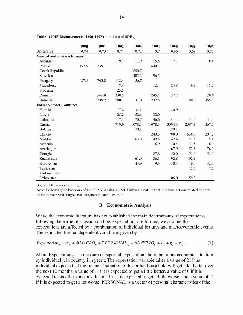
The data for IMF programs was obtained from the IMF’s “Disbursements and Repayments” available on the IMF’s website.10 IMF programs were common in the 1990s in transition economies. The IMF had programs worth over $25 billion between 1990 and 1997 (see Table 1).11 Following the fall of the “Iron Curtain,” economies in Central and Eastern Europe requested IMF programs to help them transition to market economies. The transition process involved political, institutional, and social changes, with large costs to the population. We classify transition economies according to two main groups: those that are part of Central and Eastern European and Baltic States (CEEC) and those that are part of the Commonwealth of Independent States (CIS). The former group includes Albania, Bosnia and Herzegovina, Bulgaria, Croatia, Czech Republic, Estonia, Hungary, Latvia, Lithuania, Former Yugoslav Republic of Macedonia, Poland, Romania, the Slovak Republic, Slovenia and the Former Republic of Yugoslavia. The latter group includes Armenia, Azerbaijan, Belarus, Georgia, Kazakhstan, Kyrgyzstan, Moldova, Russia, Tajikistan, Turkmenistan, Ukraine, and Uzbekistan. These two groups vary greatly in their level of GDP per capita, unemployment levels, population size, education level, and overall development (Schiff et al., 2006).

Initially, all the countries examined suffered income declines during the transition process. During the period examined, only Poland recovered the output level of 1990, with over one-third of the countries having a measured output that was still 40 percent or more below the 1989 level in 1997 (MONEE PROJECT, 1999). Most CEEC countries bottomed out around 1992-93 and CIS countries a bit later. In the first few years, the most advanced countries, which had been under communism for less time, and were in better economic positions to begin with than less-advanced countries, required IMF programs to help them make the macroeconomic adjustment. With time, countries further to the east started reforming and came under Fund programs (see Berengaut, et al., 1999). This explains why the size and the timing of IMF programs depended greatly on the initial state of the economy. According to Havrylyshyn et al. (1999) “program design has generally differed very little across [Transition] countries” [emphasis added] (p. 26), suggesting that there is little heterogeneity among IMF programs across the countries of interest.

10 See http://www.imf.org/external/np/fin/tad/extrep1.aspx

11 Structural adjustment programs have touched virtually every developing country at one time or another. According to Barro and Lee (2005), except for Botswana, Kuwait, and Malaysia, almost all developing countries have at one point been subject to an IMF program.

14

Table 1: IMF Disbursements, 1990-1997 (in million of SDRs)

1990 1991 1992 1993 1994 1995 1996 1997SDRs/US$ 0.74 0.73 0.71 0.72 0.7 0.66 0.69 0.73Central and Eastern Europe Albania 9.7 11.9 15.5 7.1 8.8 Poland 357.5 239.1 640.3 Czech Republic 850.7 Slovakia 405.2 96.5 Hungary 127.4 703.8 118.4 56.7 Macedonia 8.4 12.4 24.8 9.9 18.2 Slovenia 25.5 Romania 565.8 338.5 245.1 37.7 120.6 Bulgaria 289.2 200.3 31.0 232.5 80.0 355.2Former-Soviet Countries Estonia 7.8 34.1 20.9 Latvia 25.2 52.6 32.0 Lithuania 17.3 70.7 46.6 41.4 31.1 41.4 Russia 719.0 1078.3 1078.3 3594.3 2587.9 1467.3 Belarus 70.1 120.1 Ukraine 249.3 788.0 536.0 207.3 Moldova 63.0 49.5 42.4 22.5 15.0 Armenia 16.9 30.4 33.8 16.9 Azerbaijan 67.9 53.8 76.1 Georgia 27.8 50.0 55.5 55.5 Kazakhstan 61.9 136.1 92.8 92.8 Kyrgyzstan 43.9 9.5 30.3 16.1 32.3 Tajikistan 15.0 7.5 Turkmenistan Uzbekistan 106.0 59.3

Source: http://www.imf.org Note: Following the break-up of the SFR Yugoslavia, IMF Disbursements reflects the transactions related to debts of the former SFR Yugoslavia assigned to each Republic.

B. Econometric Analysis

While the economic literature has not established the main determinants of expectations, following the earlier discussion on how expectations are formed, we assume that expectations are affected by a combination of individual features and macroeconomic events. The estimated limited dependent variable is given by

itjtiititjitititj IMFPROPERSONALMACROnExpectatio εημβα ++++Σ+Φ+= , (7)

where Expectationitj is a measure of reported expectation about the future economic situation by individual j, in country i in year t. The expectation variable takes a value of 2 if the individual expects that the financial situation of his or her household will get a lot better over the next 12 months, a value of 1 if it is expected to get a little better, a value of 0 if it is expected to stay the same, a value of -1 if it is expected to get a little worse, and a value of -2 if it is expected to get a lot worse. PERSONAL is a vector of personal characteristics of the

15

respondent, which includes age, gender, marital status, education, employment/ unemployment (see Appendix 1 for specification and description of the data). MACRO is a vector of macroeconomic statistics of the country i in year t, and includes growth, inflation, the current account deficit as a share of GDP, as well as an index on structural reforms. We also have a dummy that separates CIS from non-CIS countries. IMF programs (IMFPRO) are considered separately for our purposes. The individual effect given by ui captures unobservable individual effects, while time effects tη captures changes that affect all individuals in year t.12

Our regressions suffer from two potential problems. First, expectations are likely to be un-trended in nature, and are likely to revert over time. We know from studies of human behavior that psychological variables tend to be stationary in the long run (Easterlin, 1974), and the same is likely to apply to expectations. Therefore, we cannot regress the expectations data on trended variables such as GDP for unit-root reasons. This problem can be partly resolved by using time and country dummies, and by differencing trended variables.

Second, macro variables such as inflation, GDP, structural reforms, current account deficits, and IMF programs are likely to be endogenous variables, and are likely to be affected by the political situation, such as the government’s reelection probability. Given that no credible macro instrument exists, we test our model using different forms of lag structure, to see whether macro forces lead expectations or not. To avoid problems of simultaneity bias, we use only personal characteristics as exogenous variables, and test macro variables both contemporaneously and with a time lag. The specification includes time dummies, which are not reported. Following di Tella, et al. (2003) we do not expect the potential of simultaneity between people’s expectations and the macroeconomic variables to be significant. First, even if expectations have a positive impact on growth (for instance through individuals investing and consuming more) this happens with a lag. Expectations, as a forward-looking measure, do not take into account the effect of IMF programs today but in the future. Similarly, the influx of money from IMF programs are unlikely to have a direct effect on the macro-variables in the same time period, but are likely to have a direct effect on expectations.

We use a (ordered) probit model, as expectations are ordinal rather than cardinal, (i.e., expectations are difficult to measure in absolute numbers like temperature, and more easy in relative numbers, such as first, second, and third.) We use a weighted ordered probit model to exploit the ranking information contained in the scaled dependent variable. The weighting variable that is applied allows for representative results on the subject level for Central and Eastern European transition economies. Furthermore, we cannot ignore clustering in the estimation model, which is likely to produce downward biased standard errors, owing to the effects of aggregate variables on individual data, as shown by Moulton (1990). In our 12 In a simple probit model, we assume that responses follow a binomial distribution. Let Y be a binary outcome variable, and let X be a vector of regressors. The probit assumes that

),'()'(1)1Pr( βφβφ iiii xxxXY =−−=== where φ is a cumulative distribution function of the standard normal distribution. The β parameters are estimated by using the method of maximum likelihood (see Greene, 2000, for an illustration).

16

regression analysis, we use a robust estimator of variance because random disturbances are potentially correlated within groups or clusters. Here, dependent refers to residents of the same country.

What type of results do we expect? The hypothesis below about what impacts people’s expectations is drawn from psychological studies on well-being. For analytical purposes, it is useful to differentiate two sets of sources: individual and macroeconomic variables. We hypothesize the following.

First, individual characteristics, such as age, gender and other socioeconomic variables are likely to affect people’s expectations about the future of the economy. From psychological studies, we know that younger people, more educated people, and males tend to have more confidence in the future, all else being equal (see, e.g. Myers, 1993), and hence should have higher positive expectations for the future.

Second, macroeconomic factors are likely to affect expectations of economic agents in the economy. We would expect higher growth rates to have a positive effect on people’s economic expectations, and higher inflation to have a negative effect (see, for example, di Tella et al., 2003). The effect of structural reforms is ambiguous. Reforms are often painful and might lead to reduced expectations. However, reforms carried out successfully could raise people’s expectations, as economic agents realize that most of the reform costs are behind, while the benefits are ahead.13 Finally, we would expect large current account deficits as a share of GDP to worsen people’s expectations.

Third, the effect of IMF programs on expectations are ambiguous. We would expect that IMF programs raise expectations via two channels. First, such programs can act as a signal that the country is pursuing sound policies (i.e., as a seal of approval). Second, the inflow of money from the IMF can have a positive impact on the economy by making adjustment easier. In this case, it is the actual amount of financing that is crucial. 14

However, IMF programs can also have a negative effect on people’s expectations about the future state of the economy. IMF programs can affect people’s expectations negatively in two ways: through income/job losses and through fewer government social services. IMF critics often claim that IMF programs reduce government spending and lead to more taxes and unemployment (Killick, 1995). As a result, one could expect declining confidence in the near future. However, the fact that reducing government spending is often a condition of IMF programs does not mean that people will be negatively affected by it if it is mostly “wasted” or goes to interest groups and not the general public. The data on expectations cannot differentiate each effect; it is therefore only possible to look at the net effect. Depending on whether the effect of IMF programs is expected to increase or reduce economic health, the

13 Note that some countries might not have experienced the initial trough because they delayed adjustment. This could be partially captured in the EBRD variable.

14 The effect of IMF programs on transition economies appears to be unique. These are among the few countries in the world, in which having a Fund program was often used as a strategy to win elections. I would like to thank Juan Zalduendo for pointing this out.

17

coefficient might be positive or negative. One should also bear in mind that, given that IMF programs tend to take effect after a crisis, agents’ expectations might already be so low that the effect of the IMF program is limited.

C. Main Results

This section presents the main results. Table 2 presents the estimated coefficient and the marginal effects for our expectations functions. We tested for several model specifications, and chose the model with the best coefficient of determination. We proceed sequentially, first taking account of demographic variables, then macroeconomic variables, and finally IMF programs. We first present a probit model, which is simple to interpret but leads to a loss of information. We then look at a multinomial probit model, which, while more difficult to interpret, uses more of the data. The results mostly support our hypothesis.

The low pseudo R-square can be explained by using (ordered) probit regressions on a psychological variable. The high residual variance is due to the fact that many individual characteristics cannot easily be observed, as individual psychological factors are difficult to measure and observe. This reflects the extent to which emotions and other components of expectations are driving the results, as opposed to the variables that are typically measured by economists, such as education, marital, employment status, or macro variables. Some people are inherently confident about the future, while others are inherently pessimistic about the outlook. Moreover, by having a heterogeneous sample of individuals in different countries, the model is less easy to fit than a sample with more homogenous observations.

Table 2 presents a simple probit model, because it can be easily interpreted, with the dependent variable taking the value 1 if respondents replied that the economy will “get a little better” or will “get much better,” and zero otherwise. The coefficients within our regression are not easy to interpret; we therefore need to look at marginal effects.15 The advantage of using a probit model is that it is simple to interpret. All the variables are significant at the 1 percent level, and have mostly the expected sign. The younger, more educated individuals as well as males have, all else being equal, more confidence in the future. Self-employed individuals, followed by individuals working in the private and public sector, also have positive expectations about the future, in contrast to the unemployed, who have bleak expectations about the future. Higher GDP growth improves economic agents’

15 The parameter estimates for discrete choice models must be transformed to yield estimates of the marginal effects (i.e., the change in predicted probability associated with changes in the explanatory variables). This is because the marginal effects are nonlinear functions of the parameter estimates and the levels of the explanatory variables, so they cannot generally be inferred directly from the parameter estimates. The marginal effect of Xj

on the conditional probability is given by jiij

ii XfXXYE

βββ

)'(),(

−=∂

∂, where dXXdFXf /)()( = is

the density function corresponding to F. Note that jβ is weighted by a factor f that depends on the values of all the regressors in X. For an illustration of how the transformation is estimated, see Greene (2000).

18

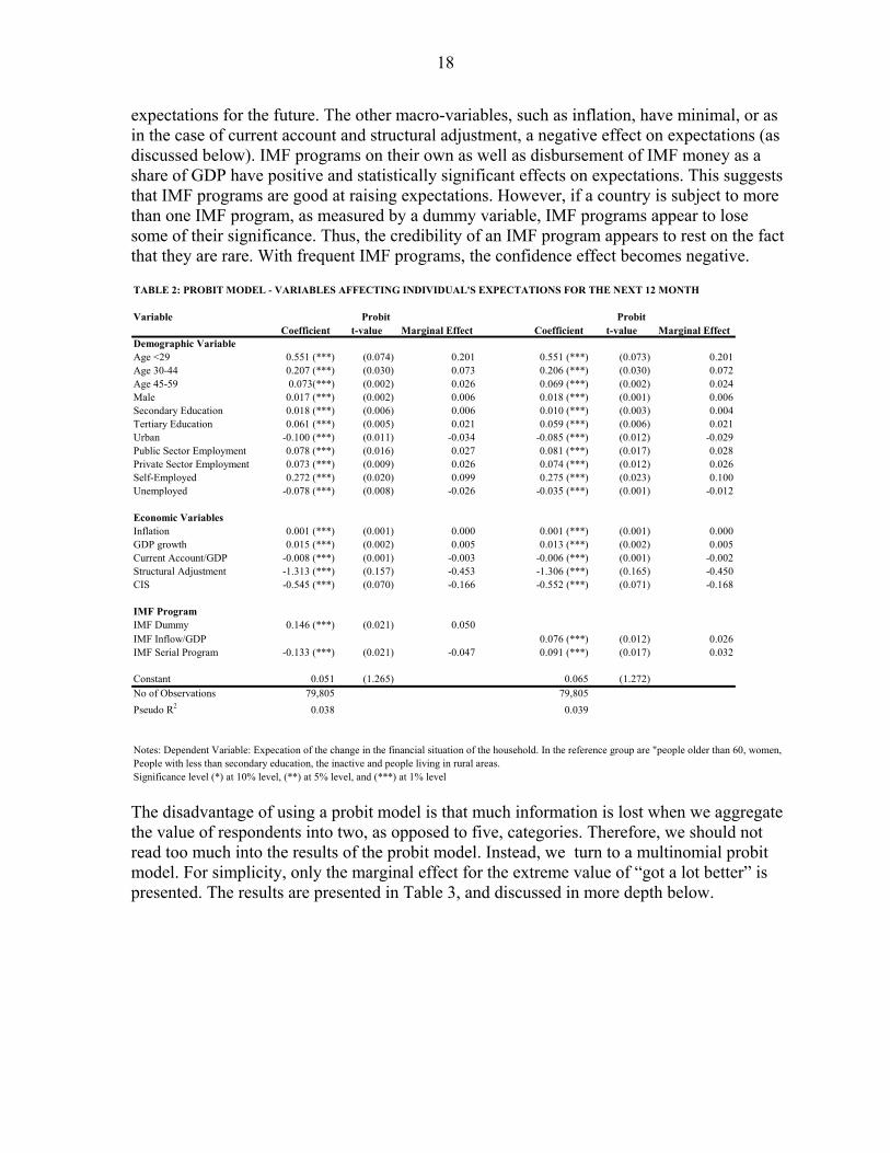
expectations for the future. The other macro-variables, such as inflation, have minimal, or as in the case of current account and structural adjustment, a negative effect on expectations (as discussed below). IMF programs on their own as well as disbursement of IMF money as a share of GDP have positive and statistically significant effects on expectations. This suggests that IMF programs are good at raising expectations. However, if a country is subject to more than one IMF program, as measured by a dummy variable, IMF programs appear to lose some of their significance. Thus, the credibility of an IMF program appears to rest on the fact that they are rare. With frequent IMF programs, the confidence effect becomes negative.

TABLE 2: PROBIT MODEL - VARIABLES AFFECTING INDIVIDUAL'S EXPECTATIONS FOR THE NEXT 12 MONTH

VariableCoefficient t-value Marginal Effect Coefficient t-value Marginal Effect

Demographic VariableAge <29 0.551 (***) (0.074) 0.201 0.551 (***) (0.073) 0.201Age 30-44 0.207 (***) (0.030) 0.073 0.206 (***) (0.030) 0.072Age 45-59 0.073(***) (0.002) 0.026 0.069 (***) (0.002) 0.024Male 0.017 (***) (0.002) 0.006 0.018 (***) (0.001) 0.006Secondary Education 0.018 (***) (0.006) 0.006 0.010 (***) (0.003) 0.004Tertiary Education 0.061 (***) (0.005) 0.021 0.059 (***) (0.006) 0.021Urban -0.100 (***) (0.011) -0.034 -0.085 (***) (0.012) -0.029Public Sector Employment 0.078 (***) (0.016) 0.027 0.081 (***) (0.017) 0.028Private Sector Employment 0.073 (***) (0.009) 0.026 0.074 (***) (0.012) 0.026Self-Employed 0.272 (***) (0.020) 0.099 0.275 (***) (0.023) 0.100Unemployed -0.078 (***) (0.008) -0.026 -0.035 (***) (0.001) -0.012

Economic VariablesInflation 0.001 (***) (0.001) 0.000 0.001 (***) (0.001) 0.000GDP growth 0.015 (***) (0.002) 0.005 0.013 (***) (0.002) 0.005Current Account/GDP -0.008 (***) (0.001) -0.003 -0.006 (***) (0.001) -0.002Structural Adjustment -1.313 (***) (0.157) -0.453 -1.306 (***) (0.165) -0.450CIS -0.545 (***) (0.070) -0.166 -0.552 (***) (0.071) -0.168

IMF ProgramIMF Dummy 0.146 (***) (0.021) 0.050IMF Inflow/GDP 0.076 (***) (0.012) 0.026IMF Serial Program -0.133 (***) (0.021) -0.047 0.091 (***) (0.017) 0.032

Constant 0.051 (1.265) 0.065 (1.272)No of Observations 79,805 79,805Pseudo R2 0.038 0.039

Significance level (*) at 10% level, (**) at 5% level, and (***) at 1% level

Probit Probit

Notes: Dependent Variable: Expecation of the change in the financial situation of the household. In the reference group are "people older than 60, women, People with less than secondary education, the inactive and people living in rural areas.

The disadvantage of using a probit model is that much information is lost when we aggregate the value of respondents into two, as opposed to five, categories. Therefore, we should not read too much into the results of the probit model. Instead, we turn to a multinomial probit model. For simplicity, only the marginal effect for the extreme value of “got a lot better” is presented. The results are presented in Table 3, and discussed in more depth below.

19

TABLE 3: ORDERED PROBIT - VARIABLES AFFECTING INDIVIDUAL'S EXPECTATIONS FOR THE NEXT 12 MONTH

VariableCoefficient t-value Marginal Effect

(score 2)Coefficient t-value Marginal Effect

(score 2)Demographic VariableAge <29 0.492 (***) (0.141) 0.045 0.489 (***) (0.140) 0.044Age 30-44 0.209 (**) (0.093) 0.016 0.207 (**) (0.093) 0.016Age 45-59 0.074 (0.056) 0.005 0.07 (0.055) 0.005Male 0.077 (***) (0.022) 0.006 0.077 (***) (0.022) 0.005Secondary Education 0.041 (**) (0.017) 0.003 0.041 (**) (0.017) 0.003Tertiary Education 0.114 (**) (0.051) 0.009 0.114 (**) (0.051) 0.009Urban -0.058 (*) (0.033) -0.004 -0.055 (*) (0.033) -0.004Public Sector Employment 0.043 (0.046) 0.003 0.047 (0.046) 0.004Private Sector Employment 0.099 (*) (0.060) 0.008 0.105 (*) (0.062) 0.008Self-Employed 0.338 (***) (0.109) 0.032 0.343 (***) (0.110) 0.033Unemployed -0.173 (*) (0.073) -0.011 -0.158 (*) (0.078) -0.010

Economic VariablesInflation 0.001 (0.003) 0.000 0.001 (0.003) 0.000GDP growth 0.016 (***) (0.004) 0.001 0.016 (***) (0.004) 0.001Current Account/GDP 0.001 (0.003) 0.000 0.001 (0.002) 0.001Structural Adjustment -0.878 (**) (0.395) -0.063 -0.876 (**) (0.385) -0.064CIS -0.487 (***) (0.121) -0.026 -0.490 (**) (0.123) -0.037

IMF ProgramIMF Dummy 0.045 (0.061) 0.003IMF Inflow/GDP 0.034 (***) (0.011) 0.002Dummy Serial Program -0.150 (**) (0.079) -0.012 -0.146 (**) (0.078) -0.012

No of Observations 79,579 79,579Pseudo R2 0.0274 0.0277

Significance level (*) at 10% level, (**) at 5% level, and (***) at 1% level

Ordered Probit Ordered Probit

Notes: Dependent Variable: Expecation of the change in the financial situation of the household. In the reference group are "people older than 60, women, People with less than secondary education, the inactive and people living in rural areas.

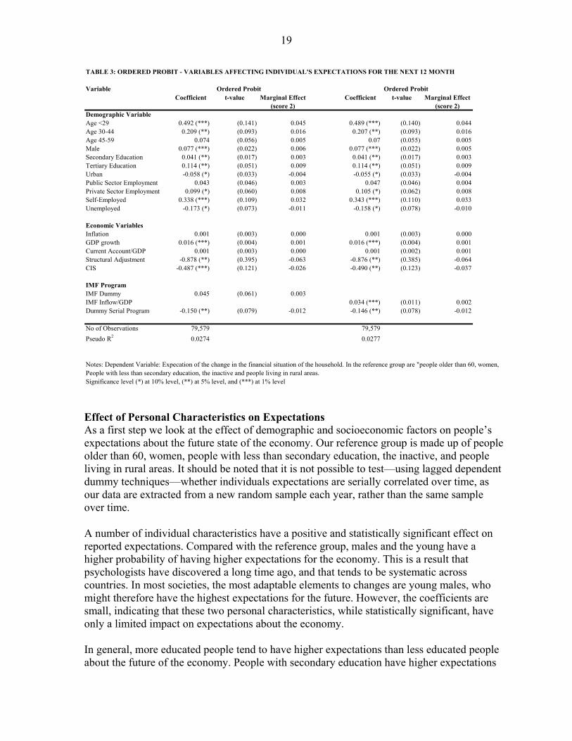
Effect of Personal Characteristics on Expectations As a first step we look at the effect of demographic and socioeconomic factors on people’s expectations about the future state of the economy. Our reference group is made up of people older than 60, women, people with less than secondary education, the inactive, and people living in rural areas. It should be noted that it is not possible to test—using lagged dependent dummy techniques—whether individuals expectations are serially correlated over time, as our data are extracted from a new random sample each year, rather than the same sample over time. A number of individual characteristics have a positive and statistically significant effect on reported expectations. Compared with the reference group, males and the young have a higher probability of having higher expectations for the economy. This is a result that psychologists have discovered a long time ago, and that tends to be systematic across countries. In most societies, the most adaptable elements to changes are young males, who might therefore have the highest expectations for the future. However, the coefficients are small, indicating that these two personal characteristics, while statistically significant, have only a limited impact on expectations about the economy. In general, more educated people tend to have higher expectations than less educated people about the future of the economy. People with secondary education have higher expectations

20

than people with primary education in a statistically significant way. People with tertiary education, in turn, are more optimistic about the future than people with secondary education, a finding that is again statistically significant. This might be because skilled people have more opportunities, both when the economy does well and when it does badly. The unemployed have a higher probability of having negative expectations about the economic future. This might be because unemployment benefits (when available) are low, and often adjust only a little to factors like changes in price levels. People working in the public sector are more likely to have positive expectations about the future of the economy, although not in a statistically significant way. Given that their positions are relatively stable, they may not fear or expect much from upswings or downswings in economic growth. Economic agents in the private sector have positive expectations about the future, which is statistically significant at the 10 percent level. This might reflect the dynamism of the private sector, with rising employment level and wages, in many of these countries. For self-employed individuals, expectations about the economy are even larger and are statistically significant at the 1 percent level, reflecting even more the perceived dynamism of the economy. Individuals living in urban areas have negative and statistically significant expectations of the future. This might be because economic agents living in rural areas are likely to be less affected by the economic situation of the country as a whole. Given that industry tends to be located in urban areas, the rural areas are less affected by the economic restructuring following the transition to capitalism. To recap, variables that are individual-specific—gender, age, education level, and employment—have consistent effects on expectations, as would have been expected from theory. Effect of Macro-Variables on Expectations We further our analysis by looking at the effect of macroeconomic variables on people’s expectations. Since people’s projections are more affected by changes in macroeconomic variables, rather than by the actual value of the macro variable, we will only look at macro changes. Do macroeconomic factors feed through into agents’ expectations about the future of the economy? We test for simultaneity between the macro-variables and confidence by lagging the independent variables. The results (not shown) do not change much, however. This suggests that our findings are relatively robust to possible problems of simultaneity. This can be explained by our dependent variable, which by definition is forward looking, and does not lead to contemporaneous changes in macroeconomic variables. Our results suggest that macroeconomic variables have a small impact on expectations, as measured by their coefficients, which is in contrast to individual factors, which have a relatively large effect on economic agents’ expectations. In general, we would expect that the pace of economic reforms, as measured by the change in the European Bank for Reconstruction and Development’s (EBRD’s) Structural Reform

21

Index,16 would have a negative short-run effect but positive long-run effect on expectations. This is because economic reforms tend to be painful. This short-run pain is indeed captured in the data, as the structural reform variables have a negative marginal effect on expectations that is statistically significant. This might be because reforms are inherently time consuming and take a long time to affect the economy. We would expect that rising inflation would reduce expectations about the future health of the economy, as it is a sign that the macroeconomic environment deteriorates, in anticipation of higher interest rates, for instance. Inflation has not a statistically significant effect on expectations. Similarly, if we lead the inflation variable (i.e., if we assume that next year’s inflation is predictable), the effect on expectations are not statistically significant (results not reported). Why is the coefficient on the inflation variable so low and statistically insignificant? We can think of two reasons. In countries that have brought inflation to low levels, inflation has little effect on expectations, as its containment is taken for granted. In countries with high levels of inflation, the inflation variable is also not significant, likely because economic agents are used to living with higher inflation and because individuals are able to circumvent this problem by, for example, using hard currencies. Moreover, wages tend to be indexed in many high-inflation countries, reducing the cost of inflation on economic agents. In both cases, the effect of inflation on expectations would therefore be lower. Economic growth has a small positive and statistically significant effect on expectations. At first, the small coefficient is surprising, as one would expect that higher growth would have a large effect on expectations. The relatively slow growth experienced by most transition economies over the 1990-97 period might have reduced the expectations of growth bringing about positive results. The rewards from higher growth did not accrue to economic agents as rapidly as in other countries. Economic agents might, for example, have found a job, but not one commensurate with their qualifications or expectations. Moreover, leading the economic growth variable (i.e., assuming economic agents can predict next year’s GDP growth) has no statistically significant effect on expectations, confirming that the GDP growth variable is not the most important variable in economic agent’s forecast of the future. Our findings also suggest that a large current account (CA) surplus as a share of GDP has a positive effect on expectations, and conversely, a CA deficit has a negative effect on expectations. The effect is, however, not statistically significant, suggesting that CA deficits in the case of transition economies were not important in affecting economic agent’s expectations. This might be because part of these CA deficits did not reflect foreign borrowing to finance consumption, but rather foreign borrowing to finance investment, and

16 The EBRD formula is made up three components. The first element is the EBRD's index for price liberalization and competition policy (accounts for 0.3), the second element is the EBRD's index for trade and foreign exchange liberalization (accounts for 0.3) and the final element is the EBRD’s index for large-scale privatization, small-scale privatization, and banking reform (accounts for 0.4). Each index is normalized and bound between 0 and 1.

22

hence was not deemed a problem by the majority of the population, as long as it was sustainable. If we group and compare Central Europe with the CIS region, we find that the CIS dummy variable is negative and statistically significant, suggesting that the public in these countries have lower expectations for the economic future. This can in part be explained by the fact that CIS countries are anticipating slower entry into the European Union than are Central European countries. Related to this, higher aid levels from the EU to Central Europe than to the CIS has helped these countries to develop faster. Finally, the population in CIS countries might anticipate that hard reforms lie ahead, which would again make agents less optimistic about the near future. To recap, in contrast to individual effects, agents’ expectations do not appear to be as affected by macroeconomic variables. Presumably, this might be because individuals adapt quickly to changes and incorporate them into their expectations. Perhaps what matters to expectations is not whether inflation/GDP growth/changes in structural adjustment/CA deficits are high or low, but rather whether each variable is above or below expectation. Effect of IMF Programs on Expectations Our main hypothesis is to test the effect of IMF programs on the public’s expectations for the economy, and to estimate the size of that effect. The issue of the timing of IMF programs and the survey are crucial. The surveys were carried out over two weeks in October/November of each year. Given that we want to test how IMF programs affect economic agent’s confidence, IMF programs were only measured if they happened in the same year prior to the survey. If IMF programs occurred after the survey, the variable for expectations used was next year’s variables. We find no evidence that this timing is significant, probably reflecting that IMF programs are anticipated in advance. By simply using a dummy-variable for years in which countries were under an IMF program, it appears that IMF programs have a positive effect on confidence, but that effect is not statistically significant, in contrast to the simple probit model, where IMF programs alone appeared to have a positive statistically significant effect on expectations (Table 2). Therefore, an IMF program as such does not raise the public’s expectations about the health of the economy, implying such programs do not have strong signaling effects. This might be a result of IMF programs in CEEC countries often having been enacted for political considerations, not necessarily economic ones (see Barro and Lee, 2003). Following the collapse of the Soviet block, Western countries did not want the CEEC region to collapse, so as to avoid them reverting back to communism. Hence, in these circumstances, when an IMF program is given despite a lack of reforms, it will not act as a seal of approval for good economic policies. In that case, it would simply reflect that the country is politically important enough to get money without actually having to carry out reforms. Given that the effectiveness of IMF programs vary from country to country, one would ideally like to have a measure of the effectiveness of IMF programs. To assess the

23

effectiveness of IMF programs, we use a dummy that differentiates countries that only had one IMF program from countries that have used IMF programs multiple times. Presumably, if a country has had only one IMF program, the program was effective. Conversely, if a country repeatedly accesses IMF funds, the implication is that the IMF program was less effective. The dummy is statistically significant and suggests that in countries where only one IMF program took place, the program had a positive effect on expectations compared with countries where several IMF programs took place. Our findings that IMF programs are not statistically significant in raising expectations change once we use a more accurate measure of IMF programs. When we use the size of IMF programs as a share of GDP as a proxy for IMF programs, the coefficient becomes large, and it has a statistically significant effect on expectations. Thus, it appears that the inflow of funds, more than the signaling effect of IMF programs, matter to expectations. This implies that IMF financing has a real positive effect on public expectations about the health of the economy, with people valuing the actual financing received from the IMF. It should be pointed out that while the effect of IMF programs measured as a share of GDP is statistically significant, the coefficient is not large.17 This finding is nonetheless significant, suggesting that the role of IMF financing can help restore the public’s confidence in the economy. By definition, for people who say they expect the economy in the next 12 months to either “get a little worse” or “get a lot worse,” the overall findings look different. The effect of IMF programs when measured as a dummy variable had a negative effect on expectations but was not statistically significant; by contrast, IMF programs when measured as a share of GDP had a negative and statistically significant effect on expectations. Thus, the effect of IMF programs IMF programs tend to reinforce an individual’s expectations for the future; it has a positive feedback effect on one’s forecast about the future. Robustness Test: Comparing 1990-93 with 1994-97 In all the transition economies, the first years of transition were difficult, with output collapsing as a result of the reorientation of the economy toward a functioning market economy. For most transition economies, output collapsed until 1993, and started to rebound thereafter. (We also tested this by breaking the sample in 1992 and 1994, but found that 1993 had the most significant results.) As a result, we split our sample into two periods, as shown in Table 4A and 4B, to see whether the IMF programs had different effects on the expectation of economic agents during that period. The results for most variables do not change significantly compared with the whole 1990-97 sample, except for our variable of interest, namely IMF programs. Interestingly, for those with strong positive expectations about the future, we find that in the early years of economic stress, it is not just the inflow of IMF money as a share of GDP that

17 This confirms also the results of Ramakrishnan and Zalduendo (2006), who look at the effect of IMF programs on crisis prevention. They use cluster analysis on 27 emerging market economies from 1994 to 2004 and find that the amount of financing from the IMF was crucial in crisis prevention, but that IMF programs was not statistically significant.

24

matters. The signaling effect of IMF programs, as measured by the IMF dummy, is itself statistically significant in the early years of transition (Table 4A). By acting as an anchor during a period of high uncertainty, and signaling that the country would be helped during its initial disorganization phase, IMF programs improved expectations for those with a confident economic outlook. By contrast for those with negative beliefs in the future, the signaling effect of an IMF program and the size of an IMF program as a share of GDP have a negative effect on expectations. This confirms the positive feedback effect that IMF programs appear to have on expectations. TABLE 4A: ORDERED PROBIT - VARIABLES AFFECTING INDIVIDUAL'S EXPECTATIONS FOR THE NEXT 12 MONTH

VariableCoefficient t-value Marginal Effect

(score 2)Coefficient t-value Marginal Effect

(score 2)Demographic VariableAge <29 0.568 (***) (0.157) 0.061 0.557 (***) (0.154) 0.059Age 30-44 0.244 (***) (0.093) 0.022 0.228 (**) (0.089) 0.020Age 45-59 0.122 (*) (0.068) 0.011 0.101 (*) (0.062) 0.009Male 0.077 (***) (0.022) 0.006 0.074 (***) (0.021) 0.006Secondary Education 0.044 (***) (0.009) 0.003 0.041 (***) (0.006) 0.003Tertiary Education 0.087 (**) (0.038) 0.007 0.090 (**) (0.037) 0.008Urban -0.148 (***) (0.050) -0.011 -0.136 (***) (0.046) -0.010Public Sector Employment 0.095 (***) (0.034) 0.008 0.098 (***) (0.034) 0.008Private Sector Employment 0.226 (***) (0.056) 0.022 0.239 (***) (0.059) 0.023Self-Employed 0.243 (***) (0.071) 0.024 0.273 (***) (0.069) 0.028Unemployed -0.056 (0.081) -0.004 -0.015 (*) (0.073) -0.001

Economic VariablesInflation 0.001 (0.001) 0.000 -0.001 (0.001) 0.000GDP growth 0.010 (**) (0.005) 0.001 0.010 (**) (0.005) 0.001Current Account/GDP -0.014 (0.006) -0.001 -0.012 (**) (0.006) -0.001Structural Adjustment -0.772 (**) (0.300) -0.063 -0.752 (**) (0.312) -0.060CIS -0.738 (***) (0.188) -0.035 -0.712 (***) (0.187) -0.034

IMF ProgramIMF Dummy 0.148 (**) (0.065) 0.001IMF Inflow/GDP 0.089 (***) (0.017) 0.007Dummy Serial Program -0.365 (**) (0.127) -0.039 -0.361 (***) (0.127) -0.038

No of Observations 24,314 24,314Pseudo R2 0.0291 0.0312

Significance level (*) at 10% level, (**) at 5% level, and (***) at 1% level

Ordered Probit 1990-1993 Ordered Probit 1990-1993

Notes: Dependent Variable: Expecation of the change in the financial situation of the household. In the reference group are "people older than 60, women, people with less than secondary education, the inactive and people living in rural areas.

. If we look at the period 1994–97, once the economic recovery is underway, we find that most of our variables of interest cease to be statistically significant. Once the output collapse is reversed, individual factors such as education, gender, employment status, and macroeconomic variables have a lower effect on economic agents’ expectations for the future. This suggests that there is a structural break, and that people’s expectations during the recovery phase are affected by new factors, with IMF programs losing their statistical significance in affecting economic agents’ expectations. It is notable that from 1994 onwards, with economic recovery well underway in most transition economies, both the signaling effect of IMF programs and the actual inflow of money as a share of GDP become

25

insignificant (Table 4B). For both economic agents with positive or negative expectations of the future, IMF programs cease to matter in forecasting the economic future. The confidence-generating effect of IMF programs was therefore important during the actual crisis period for individuals with positive beliefs in the future, but not thereafter. The opposite holds for individuals with negative perceptions about the economy, where the effect of IMF programs on expectations is negative during the crisis period but does not affect expectations in a systematically significant way once the economic collapse is over. Moreover, the frequency of IMF programs has a negative effect on expectations, suggesting that many IMF programs lower expectations for the future. TABLE 4B: ORDERED PROBIT - VARIABLES AFFECTING INDIVIDUAL'S EXPECTATIONS FOR THE NEXT 12 MONTH

VariableCoefficient t-value Marginal Effect

(score 2)Coefficient t-value Marginal Effect

(score 2)Demographic VariableAge <29 0.557 (***) (0.154) 0.031 0.385 (***) (0.118) 0.059Age 30-44 0.228 (**) (0.090) 0.003 0.044 (0.079) 0.020Age 45-59 0.101 (*) (0.062) -0.003 -0.052 (0.069) 0.009Male 0.074 (***) (0.021) 0.001 0.002 (0.055) 0.006Secondary Education 0.041 (***) (0.006) 0.008 0.121 (0.079) 0.003Tertiary Education 0.090 (**) (0.037) 0.018 0.233 (*) (0.141) 0.008Urban -0.023 (0.085) -0.002 -0.036 (0.880) -0.010Public Sector Employment 0.083 (0.053) 0.006 0.08 (0.052) 0.008Private Sector Employment 0.137 (*) (0.080) 0.010 0.132 (0.083) 0.023Self-Employed 0.370 (**) (0.160) 0.034 0.366 (**) (0.163) 0.028Unemployed -0.001 (0.001) 0.000 -0.001 (0.001) -0.001

Economic VariablesInflation 0.002 (0.001) 0.001 0.002 (0.002) 0.000GDP growth 0.034 (***) (0.010) 0.002 0.036 (***) (0.013) 0.001Current Account/GDP 0.021 (*) (0.012) 0.001 0.0182 (0.011) -0.001Structural Adjustment -0.845 (*) (0.511) -0.057 -0.926 (*) (0.539) -0.060CIS -0.230 (***) (0.073) -0.014 -0.181 (**) (0.078) -0.034

IMF ProgramIMF Dummy -0.017 (0.118) -0.001IMF Inflow/GDP -0.072 (0.054) 0.007Dummy Serial Program -0.039 (0.047) -0.003 -0.036 (0.079) -0.038

No of Observations 55,491 55,491Pseudo R2 0.0314 0.0321

Significance level (*) at 10% level, (**) at 5% level, and (***) at 1% level

Ordered Probit 1994-1997 Ordered Probit 1994-1997

Notes: Dependent Variable: Expecation of the change in the financial situation of the household. In the reference group are "people older than 60, women, people with less than secondary education, the inactive and people living in rural areas.

The policy implication is that in transition economies IMF loans appear to have a strong effect on agents’ expectations in the early years, through the inflow of real money, and through the signaling effect. They are positive for those with an optimistic outlook, but negative for those with a negative outlook. Once the recovery is underway, and economic uncertainty diminishes, IMF programs cease to have a statistically significant effect on the expectation of economic agents, regardless of their outlook. This finding is robust to changes in the econometric specifications.

26

IV. CONCLUSION

IMF programs have been heavily criticized, in part because some analysts claim that they do not improve agents’ expectations of economic outcomes. As our analysis shows, however, such studies have relied on indirect proxies to measure expectations about the economy. In this paper we rely on stated expectations of the future of the economy. This is the first paper, to our knowledge, to rely on this type analysis.

Our main finding is that the effect of IMF programs—whether measured as a dummy or as inflows of IMF loans as a share of GDP—have an effect on expectations, depending on the overall economic context. Expectations about the future of the economy rise when individuals are young, educated, male, and/or work as independents. Macroeconomic factors such as GDP growth, current account deficit, inflation, and advances toward a market economy have little or no significant effect on the public’s confidence in future economic outcomes. Our analysis also suggests that Central Eastern Europeans are also more confident about the future than individuals in CIS countries. Our results suggest that IMF programs do have a strong effect on agents’ expectations in the early years of economic collapse (1990–93), through both the inflow of real money and the signaling effect. IMF programs during periods of collapsing growth reinforce once underlying expectation in the future; indeed, they are positive for those with an optimistic outlook, but negative for those with a negative outlook. Once growth stabilizes (1994–97), and economic uncertainty diminishes, IMF programs cease to have a statistically significant effect on the expectation of economic agents, regardless of their overall outlook for the economy. IMF support only appears to matter in the early years of uncertainty. In the later years, during the recovery period, IMF support does not affect expectations. Should these results hold for other countries, they would suggests that IMF programs matter most in periods of high uncertainty and high disorganization, such as after wars, and only for people who have an optimistic outlook for the economy. Once countries recover from this period of disorganization, the effect of IMF programs on expectations are insignificant. A final interesting result is that the effect on expectations of IMF programs depends negatively on their frequency. In a country subject to several IMF programs, the effect on expectations becomes negative. This suggests a reputation effect exists in IMF programs; that is, if they do not succeed the first time, they tend to lose their credibility. Our results have to be taken with caution, however. Despite the potential contribution of relying on survey data as opposed to realized outcomes, the results are tentative, owing to potential biases in the survey data, and because of limited information of individual traits among the people surveyed. Moreover, given that transition economies are unique, the results do not necessarily apply to other regions.

27

V. REFERENCE

Barro, Robert J., and Jong-Wha Lee, 2003, “IMF Programs: Who is Chosen and What Are the Effects?” NBER Working Paper No. 8951 http://papers.nber.org/papers/w8951

Begg, David, 1982, The Rational Expectations Revolution in Macroeconomics: Theories and Evidence (Baltimore, Maryland: The Johns Hopkins University Press).

Benelli, Roberto, 2003, “Do IMF-Supported Programs Boost Private Capital Inflows? The Role of Program Size and Policy Adjustment,” IMF Working Paper No. 231.

Berengaut, Julian, Marta de Castello Branco, Oli Havrylyshyn, Valerie Mercer-Blackman, Ron van Rooden, and Thomas Wolf, 1999, “Growth Experience in Transition Courtiers, 1990–98” IMF Occasional Paper No.184.

Bertrand, Marianne, and Sendhil Mullainathan, 2001, “Do People Mean What They Say? Implications for Subjective Survey Data,” American Economic Review, Vol. 91, pp. 67-72.

Bikhchandanii, Sushil, David Hirschleifer, and Ivo Welch, 1998, “Learning from the Behavior of Others: Conformity, Fads and Informational Cascades,” Journal of Economic Perspectives, Vol. 12, pp. 151-70.

Bordo, Michael, Ashoka Mody, and Nienke Oomes, 2004, “Keeping Capital Flowing: The Role of the IMF,” IMF Working Paper No. 197.

Cagan, Phillip, 1956, “The Monetary Dynamics of Hyperinflation,” in Milton Friedman (ed.), Studies in the Quantity Theory of Money, (University of Chicago Press).

Calvo, Guillermo, and Enrique Mendoza, 2000, “A Rational Contagion and the Globalization of Securities Markets,” Journal of International Economics, Vol. 51, pp.79-113.

Central and Eastern Eurobarometer 1990-1997: Trends CEEB, “European Commission” http://www.icpsr.umich.edu/cgi-bin/bob/newark?study=4153.

Corsetti, Giancarlo, Bernardo Guimaraes, and Nouriel Roubini, 2003, “International Lending of Last Resort and Moral Hazard: A Model of IMF’s Catalytic Finance,” NBER Working Paper No. 10125 http://www.nber.org/papers/w10125.pdf. Di Tella, Rafael, Robert MacCulloch, and Andrew Oswald, 2003, “The Macroeconomics of

Happiness,” Review of Economic Statistics Vol. 85, 809-27. Easterlin, Richard, 1995, “Will Raising the Incomes of All Increase the Happiness of All?”

Journal of Economic Behavior and Organization, Vol. 27, pp. 35-48. Erev, Ido, and Brent Cohen, 1990, “Verbal versus Numerical Probabilities: Efficiency,

Biases and the Preference Paradox,” Organizational Behavior and Human Decision Processes, Vol. 45, pp. 1-18.

Ferguson, Niall (2006) "Political Risk and the International Bond Market Between the 1848 Revolution and the Outbreak of the First World War," Economic History Review 59, pp. 70-112.

Frankel, Jeffrey, 2005, “Mundell-Fleming Lecture: Contractionary Currency Crashes in Developing Countries,” IMF Staff Papers, Vol. 52, pp. 149-92.

Furman, Jason, and Joseph Stiglitz, 1998, “Economic Crises: Evidence and Insight from East Asia,” Brooking Papers on Economic Activity, Vol. 2, pp. 1-135.

Goldstein, Morris, 2000, “IMF Structural Conditionality: How Much is Too Much?” Institute of International Economics Working Paper No. 4.

Goldstein, Morris, and Peter Montiel, 1986, “Evaluating Fund Stabilization Programs with Multicountry Data: Some Methodological Pitfalls,” IMF Staff Papers, Vol. 33, pp. 304-44.

28

Greene, William H., 2000, Econometric Analysis. (New Jersey: Prentice Hall; fourth edition). Guttentag, Lack, and Richard Herring, 1984, “Credit Rationing and Financial Disorder,”

Journal of Finance, Vol. 39, pp. 1359-82. Independent Evaluation Office (IEO), 2002 International Monetary Fund: Evaluation of

Prolonged Use of IMF Resources (Washington: IMF). Kahneman, Daniel, and Amos Tversky, 1974, “Judgment under Uncertainty: Heuristics and

Biases,” Science, Vol. 185, pp. 1124-31. Khan, Mohsin, 1990, “The Macroeconomic Effects of Fund-Supported Adjustment

Programs,” IMF Staff Papers, Vol. 37, pp. 195-231. Khan, Mohsin, Peter Montiel, and Nadeem Haque (eds.), 1991, Macroeconomic Models for

Adjustment in Developing Countries” (Washington: IMF). Killick, Tony, 1995, “IMF Programs in Developing Countries – Design and Impact”

(London: Routledge). Mody, Ashoka, and Alessandro Rebucci, 2006, IMF-Supported Programs: Recent Staff

Research, (Washington: IMF). Moulton, Brent, 1990, “An Illustration of a Pitfall in Estimating the Effects of Aggregate

Variables on Micro Units,” Review of Economics and Statistics, Vol.72, pp. 334-38. MONEE PROJECT, 1999, “After the Fall: The Human Impact of Ten Years of Transition”

UNICEF, Innocenti Research Centre, Florence, available at http://www.unicef.at/shop/dbdocs/afterthefall.pdf.

Muth, J., 1961, “Rational Expectations and the Theory of Price Movements,” Econometrica, Vol. 29, pp. 315-35.

Myers, D., 1993, “The Pursuit of Happiness: Who is Happy and Why?” (New York: Avon). Knight, Frank (1921) “Risk, Uncertainty and Profit” (Boston, MA: Hughton Mifflin

Company) Radelet, Steve, and Jeffrey Sachs, 1998, “The East Asian Financial Crisis: Diagnosis,

Remedies, Prospects” Brookings Papers on Economic Activity, Vol. 1, No. ?, pp. 1-74.

Sargent, Thomas, 1993, “Bounded Rationality in Macroeconomics” (Oxford: Clarendon Press).

Savage, Leonard, 1954, “The Foundations of Statistics” (New York: John Wiley & Sons). Scharfstein, David. and Jeremy Stein, 1990, “Herd Behavior and Investment,” American

Economic Review, Vol. 80, pp. 465-79. Schiff, Jerald, Philippe Egoume-Bossogo, Miho Ihara, Testsuya Konuki, and Kornelia

Krajnyak, 2006, “Labor Market Performance in Transition: The Experience of Central and Eastern European Countries,” IMF Occasional Paper No. 248.

Sheffrin, Steven, 1983, “Rational Expectations,” Cambridge Surveys of Economic Literature (Cambridge: Cambridge University Press).

Shiller, Robert, 1981, “Do Stock Prices Move too Much to be Justified by Subsequent Changes in Dividends?” American Economic Review, Vol. 71, pp. 421-36.

Simon, Herbert (1955) “A Behavioral Model of Rational Choice” Quarterly Journal of Economics, Vol. 69, pp. 99–118

Surowiecki, J., 2004, The Wisdom of the Crowds: Why the Many Are Smarter Than the Few and How Collective Wisdom Shapes Business, Economies, Societies and Nations (New York: Doubleday).

29

Thaler, Richard, 2000, “From Homo Economicus to Homo Sapiens,” Journal of Economic Perspectives, Vol. 14, pp. 133-41.

Ul Haque, Nadeem, and Mohsin Khan, 1998, “Do IMF-Supported Programs Work? A Survey of the Cross-Country Empirical Evidence,” IMF Working Paper No. 169.

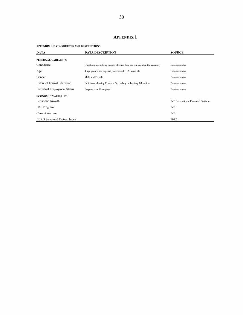
30

APPENDIX 1

APPENDIX 1: DATA SOURCES AND DESCRIPTIONS

DATA DATA DESCRIPTION SOURCE

PERSONAL VARIABLES

Confidence Questionnaire asking people whether they are confident in the economy Eurobarometer

Age 4 age groups are explicitly accounted: 1-20 years old Eurobarometer

Gender Male and Female Eurobarometer

Extent of Formal Education Indidivuals having Primary, Secondary or Tertiary Education Eurobarometer

Individual Employment Status Employed or Unemployed Eurobarometer

ECONOMIC VARIBALES

Economic Growth IMF International Financial Statistics

IMF Program IMF

Current Account IMF

EBRD Structural Reform Index EBRD