Effect of Multicolinearity and Autocorrelation on Predictive Ability

Mathematical Theory and Modeling www.iiste.org

ISSN 2224-5804 (Paper) ISSN 2225-0522 (Online)

Vol.2, No.11, 2012

41

Effect of Multicolinearity and Autocorrelation on Predictive Ability

of Some Estimators of Linear Regression Model

Kayode Ayinde1*

R. F. Alao2 Femi J. Ayoola

2

1. Department of Statistics, Ladoke Akintola University of Technology

P. M. B. 4000, Ogbomoso, Oyo State,, Nigeria.

2. Department of Statistics, University of Ibadan, Oyo State, Nigeria.

*E-mail: [email protected], or [email protected]

Abstract

Violation of the assumptions of independent regressors and error terms in linear regression model has respectively

resulted into the problems of multicollinearity and autocorrelation. Each of these problems separately has significant

effect on parameters estimation of the model parameters and hence prediction. This paper therefore attempts to

investigate the joint effect of the existence of multicollinerity and autocorrlation on Ordinary Least Square (OLS)

estimator, Cochrane-Orcutt (COR) estimator, Maximum Likelihood (ML) estimator and the estimators based on

Principal Component (PC) analysis on prediction of linear regression model through Monte Carlo studies using the

adjusted coefficient of determination goodness of fit statistic of each estimator. With correlated normal variables as

regressors, it further identifies the best estimator for prediction at various levels of sample sizes (n), multicollinearity

)( and autocorrlation )( . Results reveal the pattern of performances of COR and ML at each level of

multicollinearity over the levels of autocorrelation to be generally and evidently convex especially when 30n

and 0 while that of OLS and PC is generally concave. Moreover, the COR and ML estimators perform

equivalently and better; and their performances become much better as multicollinearity increases. The COR

estimator is generally the best estimator for prediction except at high level of multicollinearity and low levels of

autocorrelation. At these instances, the PC estimator is either best or competes with the COR estimator. Moreover,

when the sample size is small (n=10) and multicollinearity level is not high, the OLS estimator is best at low level of

autocorrelation whereas the ML is best at moderate levels of autocorrelation.

.Keywords: Prediction, Estimators, Linear Regression Model, Multicollinearity, Autocorrelation.

1.0 Introduction

In linear regression analysis modeling of business, economic and social sciences data, the dependence of regressors

often leads to the problem of multcollinearity. For instance, the independent variables such as family income and

assets or store sales and number of employees or age and years of experience would tend to be highly correlated.

With strongly interrelated regressors, the regression coefficients provided by the OLS estimator are no longer stable

even though they are still unbiased as long as multicollinearity is not perfect. Furthermore, the regression coefficients

may have large sampling errors which affect both the inference and forecasting that is based on the model

(Chartterjee et al., 2000). Various other estimation methods have been developed to tackle this problem. These

estimators include Ridge Regression estimator developed by Hoerl (1962) and Hoerl and Kennard (1970), Estimator

based on Principal Component Regression suggested by Massy (1965), Marquardt (1970) and Bock, Yancey and

Judge (1973), Naes and Marten (1988), and method of Partial Least Squares developed by Hermon Wold in the

1960s (Helland, 1988, Helland, 1990, Phatak and Jony 1997).

The dependence of error terms, as often being found in time series data, leads to be problem of autocorrelated

error terms of regression model. Several authors have worked on this problem especially in terms of the parameter

estimation of the linear regression model when the error term follows autoregressive of orders one. The OLS estimator

is inefficient even though unbiased. Its predicted values are also inefficient and the sampling variances of the

autocorrelated error terms are known to be underestimated causing the t and the F tests to be invalid (Johnston, 1984;

mailto:[email protected]

mailto:[email protected]



Vol.2, No.11, 2012

42

Fomby et al., 1984; Chartterjee, 2000; Maddala, 2002). To compensate for the lost of efficiency, several feasible

generalized least squares (GLS) estimators have been developed. These estimators include those provided by Cochrane

and Orcutt (1949), Paris and Winstern (1954), Hildreth and Lu (1960), Durbin (1960), Theil (1971), the maximum

likelihood and the maximum likelihood grid (Beach and Mackinnon, 1978), and Thornton (1982). Chipman (1979),

Kramer (1980), Kleiber (2001), Iyaniwura and Nwabueze (2004), Nwabueze ( 2005a, b,c), Ayinde and Ipinyomi

(2007) and many other authors have not only observed the asymptotic equivalence of some of these estimators but

have also noted that that their performances and efficiency depend on the structure of the regressor used. Rao and

Griliches (1969) did one of the earliest Monte-Carlo investigations on the small sample properties of several two-stage

regression methods in the context of autocorrelation error. Other recent works done on these estimators include that of

Iyaniwura and Olaomi (2006), Ayinde and Oyejola (2007), Ayinde (2007a, b), Ayinde and Olaomi (2008), Ayinde

(2008), and Ayinde and Iyaniwura (2008).

In spite of these several works on these estimators, none has actually studied these estimators especially in term of

their predictive ability when both multicollinearity and autocorrelation together. More so, situations where the two

problems exist together in a data set are not uncommon. Therefore, this paper attempts to investigate the predictive

ability / potential of some of these estimators under the joint existence of these problems through Monte Carlo studies.

2.0 Materials and Methods

Consider the linear regression model is of the form:

ttttt uXXXY 3322110 (1)

Where ttt uu 1 , ),0(~ 2 Nt , t = 1, 2, 3,...n and ) i = 1, 2, 3 are

fixed and correlated.

For Monte-Carlo simulation study, the parameters of equation (1) were specified and fixed as β0 = 4, β1 = 2.5, β2 = 1.8

and β3 = 0.6. The levels of multicollinearity among the independent variables were sixteen (16) and specified

as: .99.0,9.0,8.0,...,3.0,4.0,49.0)()()( 231312 xxx The levels of autocorrelation is twenty-one

(21) and are specified as: .99.0,9.0,8.0,...,8.0,9.0,99.0 Furthermore, the experiment was replicated

in 1000 times (R =1000) under Six (6) levels of sample sizes (n =10, 15, 20, 30, 50, 100). The correlated normal

regressors were generated by using the equations provided by Ayinde (2007) and Ayinde and Adegboye (2010) to

generate normally distributed random variables with specified intercorrelation. With P= the equations give:

X1 = µ1 + σ1Z1

X2 = µ2 + ρ12 σ2Z1 + Z2 (2)

X3 = µ3 + ρ13 σ3Z1 + Z2 + Z3

Where m22 = , m23 = and n33 = m33 - ;

and Zi N (0, 1) i = 1, 2, 3. (The inter-correlation matrix has to be positive definite and hence, the correlations

among the independent variable were taken as prescribed earlier). In the study, we assumed Xi N (0, 1), i = 1, 2, 3

as earlier mentioned.

The error terms were generated using one of the distributional properties of the autocorrelated error terms

(ut N (0, )) and the AR(1) equation as follows:

u1= (3)

ut = ρut-1 + εt t = 2,3,4,…n (4)

Since some of these estimators have now been incorporated into the Time Series Processor (TSP 5.0, 2005) software,

a computer program was written using the software to estimate the Adjusted Coefficient of Determination of the

model )(

2_

R the Ordinary Least Square (OLS) estimator, Cochrane orcutt (COR) estimator, Maximum Likelihood

estimator and the estimator based on Principal Component Analysis (PRN). The Adjusted Coefficient of

Determination of the model was averaged over the numbers of replications. i.e.

R

i

iRR

R1

2_1 (5)

The two possible PCs (PC1 and PC2) of the Principal Component Analysis were used. Each provides its



Vol.2, No.11, 2012

43

separate Adjusted Coefficient of Determination. An estimator is best if its Adjusted Coefficient of Determination is

closest to unity.

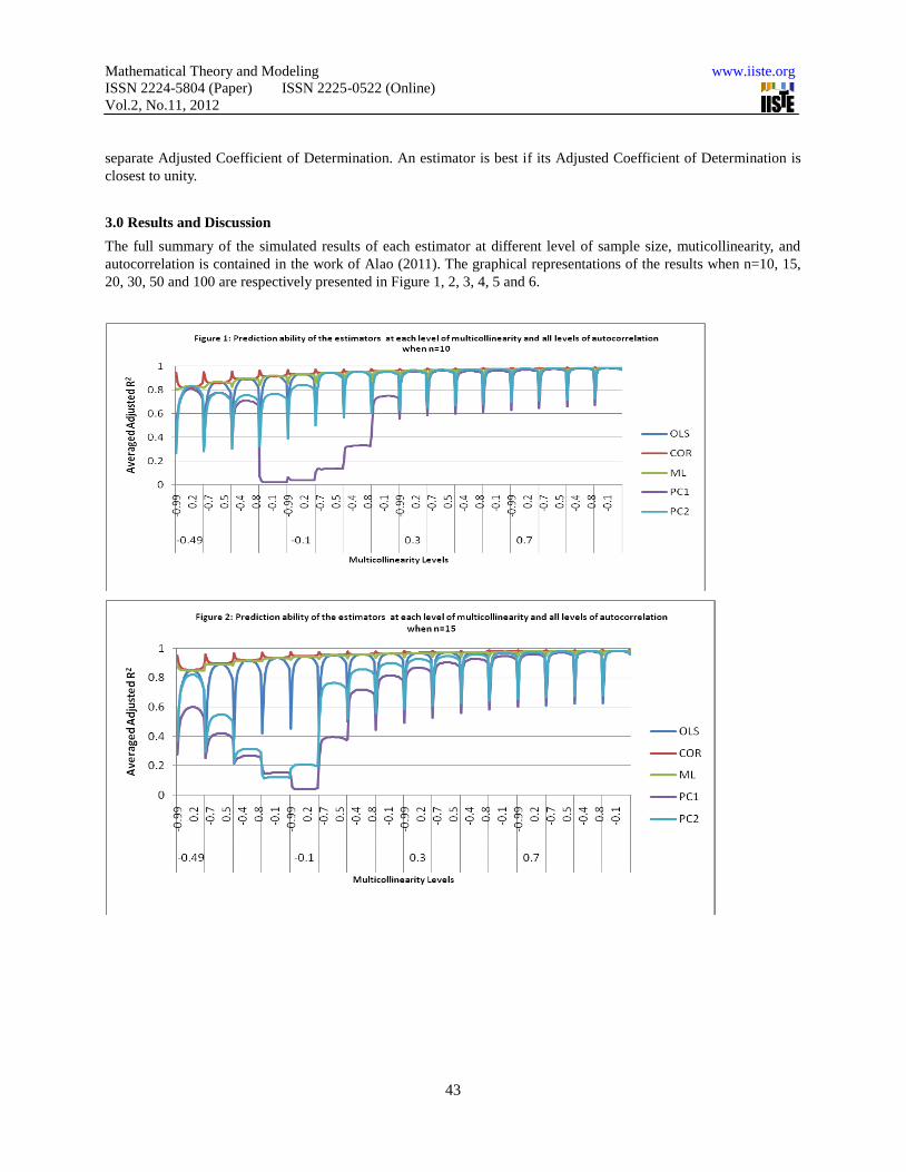
3.0 Results and Discussion

The full summary of the simulated results of each estimator at different level of sample size, muticollinearity, and

autocorrelation is contained in the work of Alao (2011). The graphical representations of the results when n=10, 15,

20, 30, 50 and 100 are respectively presented in Figure 1, 2, 3, 4, 5 and 6.



Vol.2, No.11, 2012

44



Vol.2, No.11, 2012

45

From these figures, results reveal the pattern of performances of COR and ML at each level of multicollinearity over

the levels of autocorrelation to be generally and evidently convex especially when 30n and 0 while that

of OLS and PC is generally concave. Moreover, the COR and ML estimators perform equivalently and better in that

the values of their averaged adjusted coefficient of determination are often greater than 0.8; and their performances

become much better as multicollinearity increases. The COR estimator is generally the best estimator for prediction

except at high level of multicollinearity and low levels of autocorrelation. At these instances, the PC estimator is

either best or competes with the COR estimator. Moreover when the sample size is small (n=10) and

multicollinearity level is not high, the OLS estimator is best at low level of autocorrelation whereas the ML is best at

moderate levels of autocorrelation.

Very specifically in term of identification of the best estimator, Table 1, 2, 3, 4, 5 and 6 respectively summarize

the best estimator for prediction at all the levels of autocorrelation and multicollinearity when the sample size is 10,

15, 20, 30, 50, 100.

Table 1: The Best Estimator for Prediction at different level of Multicollinearity and Autocorrelation

when n=10.

-0.49 -0.4 -0.3 -0.2 -0.1 0 0.1 0.2 0.3 0.4 0.5 0.6 0.7 0.8 0.9 0.99

-0.99 COR COR COR COR COR COR COR COR COR COR COR COR COR COR COR COR






-0.4 ML ML ML ML ML ML ML ML ML COR COR COR COR COR COR COR

-0.3 ML ML ML ML ML ML ML ML ML ML ML ML ML PC2 PC2 PC2



Vol.2, No.11, 2012

46

-0.2 ML ML ML ML ML ML ML ML ML ML ML ML PC2 PC2 PC2 PC2

-0.1 ML ML ML ML ML ML ML ML ML ML ML PC2 PC2 PC2 PC2 PC2

0 OLS OLS OLS OLS OLS OLS OLS OLS OLS OLS OLS PC2 PC2 PC2 PC2 PC2

0.1 OLS OLS OLS OLS OLS OLS OLS OLS OLS OLS OLS PC2 PC2 PC2 PC2 PC2

0.2 PC2 OLS OLS OLS OLS OLS OLS OLS OLS OLS OLS PC2 PC2 PC2 PC2 PC2

0.3 PC2 ML ML ML ML ML ML ML ML ML ML PC2 PC2 PC2 PC2 PC2

0.4 ML ML ML ML ML ML ML ML ML ML ML ML PC2 PC2 PC2 PC2

0.5 ML ML ML ML ML ML ML ML ML ML ML ML PC2 PC2 PC2 PC2

0.6 COR ML ML ML ML ML ML ML ML ML ML ML ML ML PC2 PC2

0.7 COR COR COR COR COR COR COR COR COR COR COR COR COR COR COR COR




From Table 1 when n = 10, the COR estimator is best except when 5.04.0 . When 6.0 at these

instances, the PC2 estimator is most frequently best and when the COR or ML is best, the PC2 estimator competes

very favorably. Furthermore when 5.0 , the ML estimator is best when 1.04.0 and

6.03.0 while the OLS estimator is best when 3.00 . Moreover, the PC2 estimator is still best

when 49.0 and 3.02.0 .


when n=15.

-0.49 -0.4 -0.3 -0.2 -0.1 0 0.1 0.2 0.3 0.4 0.5 0.6 0.7 0.8 0.9 0.99





0.-6 COR COR COR COR COR COR COR COR COR COR COR COR COR COR COR COR





-0.1 COR COR COR COR COR COR COR COR COR COR COR COR COR COR COR PC2

0 COR COR COR COR COR COR COR COR COR COR COR COR COR COR PC2 PC2

0.1 COR COR COR COR COR COR COR COR COR COR COR COR COR COR PC2 PC2

0.2 COR COR COR COR COR COR COR COR COR COR COR COR COR COR COR PC2

0.3 COR COR COR COR COR COR COR COR COR COR COR COR COR COR COR PC2





Vol.2, No.11, 2012

47






When n=15, the COR estimator is generally best except when 3.01.0 and 1 . At these instances,

the PC2 estimator is most frequently best and when the COR is best, the PC2 estimator competes very favorably.


when n=20.

-0.49 -0.4 -0.3 -0.2 -0.1 0 0.1 0.2 0.3 0.4 0.5 0.6 0.7 0.8 0.9 0.99










-0.1 COR COR COR COR COR COR COR COR COR COR COR COR PC2 PC2 PC2 PC2

0 COR COR COR COR COR COR COR COR COR COR COR PC2 PC2 PC2 PC2 PC2

0.1 COR COR COR COR COR COR COR COR COR COR COR PC2 PC2 PC2 PC2 PC2

0.2 COR COR COR COR COR COR COR COR COR COR COR PC2 PC2 PC2 PC2 PC2









When n=20, the COR estimator is generally best except when 2.01.0 and 6.0 . At these instances,

the PC2 estimator is most frequently best and when the COR is best, the PC2 estimator competes very favorably.



Vol.2, No.11, 2012

48


when n=30.

-0.49 -0.4 -0.3 -0.2 -0.1 0 0.1 0.2 0.3 0.4 0.5 0.6 0.7 0.8 0.9 0.99










-0.1 COR COR COR COR COR COR COR COR COR COR COR COR COR COR COR PC2

0 COR COR COR COR COR COR COR COR COR COR COR COR COR PC2 PC2 PC2

0.1 COR COR COR COR COR COR COR COR COR COR COR COR COR COR PC2 PC2










When n=30, the COR estimator is generally best except when 1.00 and 8.0 . At these instances, the

PC2 estimator is most frequently best and when the COR is best, the PC2 estimator competes very favorably.



Vol.2, No.11, 2012

49

Table 5: The Best Estimator for Prediction at different level of Multicollinearity and Autocorrelation when

n=50.

-0.49 -0.4 -0.3 -0.2 -0.1 0 0.1 0.2 0.3 0.4 0.5 0.6 0.7 0.8 0.9 0.99











0 COR COR COR COR COR COR COR COR COR COR COR COR COR COR COR PC1












when n=100.

-0.49 -0.4 -0.3 -0.2 -0.1 0 0.1 0.2 0.3 0.4 0.5 0.6 0.7 0.8 0.9 0.99











Vol.2, No.11, 2012

50



0 COR COR COR COR COR COR COR COR COR COR COR COR COR COR COR PC2











When 50n , the COR estimator is generally best except when there is no autocorrelation at all and 1 . At

these instances, the PC estimator is best.

4.0 Conclusions

The effect of two major problems, Multicollinearity and autocorrelation, on the predictive ability of the OLS, COR,

ML and PC estimators of linear regression model has been jointly examined in this paper. Results reveal the pattern

of performances of COR and ML at each level of multicollinearity over the levels of autocorrelation to be generally

and evidently convex especially when 30n and 0 while that of OLS and PC is generally concave.

Moreover, the COR and ML estimators perform equivalently and better; and their performances become much better

as multicollinearity increases. The COR estimator is generally the best estimator for prediction except at high level of

multicollinearity and low levels of autocorrelation. At these instances, the PC estimator is either best or competes

with the COR estimator. Moreover when the sample size is small (n=10) and multicollinearity level is not high, the

OLS estimator is best. at low level of autocorrelation whereas the ML is best at moderate levels of autocorrelation.

References

Alao, R. F. (2011). Estimators of Linear Regression Model with Autocorrelated Error term and Correlated Fixed

Normal Regressors. Unpublished M.Sc. Thesis. University of Ibadan, Nigeria.

Ayinde, K. (2007). Equations to generate normal variates with desired intercorrelation matrix. International Journal

of Statistics and System, 2 (2), 99 –111.

Ayinde, K. (2007). A Comparative Study of the Performances of the OLS and Some GLS Estimators When

Stochastic Regressors Are both Collinear and Correlated with Error Terms. Journal of Mathematics and Statistics,

3(4), 196 –200.

Ayinde, K. (2008). Performances of Some Estimators of Linear Model when Stochastic Regressors are correlated

with Autocorrelated Error Terms. European Journal of Scientific Research, 20 (3), 558-571.

Ayinde, K. and Adegboye, O. S. (2010). Equations for generating normally distributed random variables with

specified intercorrelation. Journal of Mathematical Sciences, 21(2), 183–203.

Ayinde, K. and Ipinyomi, R. A. (2007). A comparative study of the OLS and some GLS estimators when normally

distributed regressors are stochastic,.Trend in Applied Sciences Research, 2(4), 354-359.



Vol.2, No.11, 2012

51

Ayinde, K. and Iyaniwura, J.O. (2008). A Comparative study of the Performances of Some Estimators of Linear

Model with fixed and stochastic regressors. Global Journal of Pure and Applied Sciences, 14(3), 363–369.

Ayinde, K. and Oyejola, B. A. (2007). A comparative study of performances of OLS and some GLS estimators when

stochastic regressors are correlated with error terms. Research Journal of Applied Sciences, 2, 215–220.

Beach, C. M. and Mackinnon, J. S. (1978). A Maximum Likelihood Procedure regression with autocorrelated errors.

Econometrica, 46, 51 – 57.

Bock, M. E., Yancey, T. A. and Judge, G. G. (1973). Statistical consequences of preliminary test estimation in

regression. Journal of the American Statistical Association, 60, 234 – 246.

Chartterjee, S., Hadi, A.S. and Price, B. (2000). Regression by Example, 3rd

Edition, A Wiley-Interscience

Publication,.John Wiley and Sons..

Chipman, J. S. Efficiency of Least Squares Estimation of Linear Trend when residuals are autocorrelated,

Econometrica, 47(1979),115 -127.

Cocharane, D. and Orcutt, G.H. (1949). Application of Least Square to relationship containing autocorrelated error

terms. Journal of American Statistical Association, 44,32–61.

Durbin, J (1960). Estimation of Parameters in Time series Regression Models. Journal of Royal Statistical Society B,

22, 139 -153.

Formy, T. B., Hill, R. C. and Johnson, S. R. (1984). Advance Econometric Methods. Springer-Verlag, New York,

Berlin, Heidelberg, London, Paris, Tokyo.

Helland, I. S. (1988). On the structure of partial least squares regression. Communication is Statistics, Simulations and

Computations, 17, 581 – 607.

Helland, I. S. (1990). Partial least squares regression and statistical methods. Scandinavian Journal of Statistics, 17, 97

– 114.

Hoerl, A. E. (1962). Application of ridge analysis to regression problems. Chemical Engineering Progress, 58, 54 – 59.

Hoerl, A. E. and Kennard, R. W. (1970). Ridge regression biased estimation for non-orthogonal

problems,.Technometrics, 8, 27 – 51.

Hildreth, C. and Lu, J.Y. (1960). Demand relationships with autocorrelated disturbances. Michigan State University,

Agricultural Experiment Statistical Bulletin, 276 East Lansing, Michigan.

Iyaniwura, J.O. and Nwabueze, J. C. (2004). Estimators of Linear model with Autocorrelated error terms and trended

independent variable. Journal of Nigeria Statistical Association,17, 20 – 28.

Iyaniwura, J.O. and Olaomi, J.O. (2006). Efficiency of the GLS estimators in linear regression with autocorrelated

error terms which are correlated with regressors. Science Focus, 11,129 – 133.

Johnston, J. (1984). Econometric Methods. 3rd

Edition, New York, Mc, Graw Hill.

Kramer, W. (1980). Finite sample efficiency of OLS in linear regression model with autocorrelated errors,.Journal of

American Statistical Association, 81, 150 – 154.

Kleiber, C. (2001). Finite sample efficiency of OLS in linear regression model with long memory disturbances.

Economic Letters, 72, 131 – 136.

Maddala, G. S. (2002). Introduction to Econometrics. 3rd

Edition, John Willey and Sons Limited, England.

Marquardt, D. W. (1970). Generalized inverse, Ridge Regression, Biased Linear Estimation and Non – linear

Estimation. Technometrics, 12, 591– 612.

Massy, W. F. (1965). Principal Component Regression in exploratory statistical research. Journal of the American

Statistical Association, 60, 234– 246.

Naes, T. and Marten, H. (1988). Principal Component Regression in NIR analysis: View points, Background Details

Selection of components. Journal of Chemometrics, 2, 155 – 167.

Neter, J. and Wasserman, W. ( 1974). Applied Linear Model. Richard D. Irwin, Inc..



Vol.2, No.11, 2012

52

Nwabueze, J.C. (2005a). Performances of Estimators of linear model with auto-correlated error terms when

independent variable is normal. Journal of Nigerian Association of Mathematical Physics, 9, 379 – 384.

Nwabueze, J.C. (2005b). Performances of Estimators of linear model with auto-correlated error terms with

exponential independent variable. Journal of Nigerian Association of Mathematical Physics, 9, 385 – 388.

Nwabueze, J.C. (2005c). Performances of Estimators of linear model with auto-correlated error terms when the

independent variable is autoregressive. Global Journal of Pure and Applied Sciences, 11, 131 - 135.

Paris, S. J. and Winstein, C. B. (1954). Trend estimators and serial correlation. Unpublished Cowles Commision,

Discussion Paper, Chicago.

Phatak, A. and Jony, S. D. (1997). The geometry of partial least squares. Journal of Chemometrics, 11, 311 – 338.

Rao, P. and Griliches, Z. (1969). Small sample properties of several two-stage regression methods in the context of

autocorrelation error. Journal of American Statistical Association, 64, 251 – 272.

Theil, H.( 1971). Principle of Econometrics. New York, John Willey and Sons,.

Thornton, D. L. (1982). The appropriate autocorrelation transformation when autocorrelation process has a finite past.

Federal Reserve Bank St. Louis, 82 – 102.

This academic article was published by The International Institute for Science,

Technology and Education (IISTE). The IISTE is a pioneer in the Open Access

Publishing service based in the U.S. and Europe. The aim of the institute is

Accelerating Global Knowledge Sharing.

More information about the publisher can be found in the IISTE’s homepage:

http://www.iiste.org

CALL FOR PAPERS

The IISTE is currently hosting more than 30 peer-reviewed academic journals and

collaborating with academic institutions around the world. There’s no deadline for

submission. Prospective authors of IISTE journals can find the submission

instruction on the following page: http://www.iiste.org/Journals/

The IISTE editorial team promises to the review and publish all the qualified

submissions in a fast manner. All the journals articles are available online to the

readers all over the world without financial, legal, or technical barriers other than

those inseparable from gaining access to the internet itself. Printed version of the

journals is also available upon request of readers and authors.

IISTE Knowledge Sharing Partners

EBSCO, Index Copernicus, Ulrich's Periodicals Directory, JournalTOCS, PKP Open

Archives Harvester, Bielefeld Academic Search Engine, Elektronische

Zeitschriftenbibliothek EZB, Open J-Gate, OCLC WorldCat, Universe Digtial

Library , NewJour, Google Scholar

http://www.iiste.org/

http://www.iiste.org/Journals/

Documents

Effect of Multicolinearity and Autocorrelation on Predictive Ability