Embed Size (px)
Citation preview
1
EFFECT OF PROCESS PARAMETERS ON TEMPERATURE DISTRIBUTION
DURING FRICTION STIR WELDING
A PROJECT REPORT
SUBMITTED BY
AAYUSH TRIPATHI -CB.EN.U4MEE11103
VENKATA PRITHVI PUPPALA -CB.EN.U4MEE11160
A. SRI PRUDHVI -CB.EN.U4MEE11202
CH. VARUN TEJA -CB.EN.U4MEE11216
In partial fulfillment for the award of the degree
of
BACHELOR OF TECHNOLOGY
in
MECHANICAL ENGINEERING
DEPARTMENT OF MECHANICAL ENGINEERING
AMRITA SCHOOL OF ENGINEERING
AMRITA VISHWA VIDYAPEETHAM
COIMBATORE-641112,
MAY, 2015
2
AMRITA SCHOOL OF ENGINEERING
AMRITA VISHWA VIDYAPEETHAM, COIMBATORE – 641112
DEPARTMENT OF MECHANICAL ENGINEERING
BONAFIDE CERTIFICATE
This is to certify that the thesis entitled “EFFECT OF PROCESS PARAMETERS ON
TEMPERATURE DISTRIBUTION DURING FRICTION STIR WELDING”
submitted by AAYUSH TRIPATHI (CB.EN.U4MEE11103), VENKATA PRITHVI
PUPPALA (CB.EN.U4MEE11160), A. SRI PRUDHVI (CB.EN.U4MEE11202) and
CH. VARUN TEJA (CB.EN.U4MEE11216) for the award of the Degree of Bachelor
of Technology in Mechanical Engineering is a bonafide record of the work carried out
under the my/ our guidance and supervision at Amrita School of Engineering,
Coimbatore.
Dr. R.Padmanaban
Project Advisor
Dept. of Mechanical Engineering
Amrita School of Engineering
Dr. S. Thirumalini
Chairperson
Dept. of Mechanical Engineering
Amrita School of Engineering
This report was examined and the candidates underwent Viva- Voce examination on
____________.
Internal Examiner External Examiner
3
AMRITA SCHOOL OF ENGINEERING
AMRITA VISHWA VIDYAPEETHAM, COIMBATORE – 641112
DEPARTMENT OF MECHANICAL ENGINEERING
DECLARATION
We AAYUSH TRIPATHI (CB.EN.U4MEE11103), VENKATA PRITHVI
PUPPALA (CB.EN.U4MEE11160), A. SRI PRUDHVI (CB.EN.U4MEE11202) and
CH. VARUN TEJA (CB.EN.U4MEE11216) hereby declare that the project work
entitled “EFFECT OF PROCESS PARAMETERS ON TEMPERATURE
DISTRIBUTION DURING FRICTION STIR WELDING”, is the record of the
original work done by us, under the guidance of Dr. R. PADMANABAN, Department of
Mechanical Engineering. To the best of our knowledge this work has not formed the
basis for the award of any degree/ diploma/ associateship/ fellowship or a similar award
to any candidate in any university.
AAYUSH TRIPATHI VENKATA PRITHVI PUPPALA
A.SRI PRUDHVI CH.VARUN TEJA
Place: Coimbatore, 641112
Date:
COUNTERSIGNED
Dr. R. PADMANABAN
Project Advisor
Dept. of Mechanical Engineering
Amrita School of Engineering
4
ACKNOWLEDGEMENT
There has been a great many people that have played a part in the completion of this
work. Each has contributed in different but equally important ways that must be
acknowledged.
This report is the final year project submitted to the Mechanical Engineering Department
of Amrita School of Engineering. My supervisor, Dr. R. Padmanaban has played a large
role and must be thanked for his guidance and invaluable help throughout the period of
this work.
We would finally like to acknowledge the Amrita School of Engineering for the support
over the duration of this work. Our gratitude goes to all the CAD lab assistants and the
faculty of the Department of Mechanical Engineering for their timely help and valuable
inputs.
Aayush Tripathi
Venkata Prithvi Puppala
A. Sri Prudhvi
Ch. Varun Teja
5
Contents
ABSTRACT ...................................................................................................................... 10
CHAPTER 1 Introduction................................................................................................. 11
1.1 Friction Stir Welding ............................................................................................... 11
1.2 Advantages of FSW ................................................................................................ 12
1.3 Disadvantages of FSW ............................................................................................ 12
1.4 Industrial Applications ............................................................................................ 13
1.4.1 Shipbuilding and Marine Construction ............................................................. 13
1.4.2 Aerospace Industry ........................................................................................... 14
1.4.3 Railway Industry............................................................................................... 15
1.4.4Land Transportation .......................................................................................... 15
1.5 PROCESS PARAMETERS .................................................................................... 16
1.5.1 Tool Geometry .................................................................................................. 16
1.5.2. Welding Parameters ......................................................................................... 17
1.5.3 Joint Design ...................................................................................................... 18
1.6 Objective ................................................................................................................. 19
CHAPTER 2: LITERATURE SURVEY.......................................................................... 20
2.2 Residual Stress ........................................................................................................ 24
2.3 Temperature Distribution ........................................................................................ 28
CHAPTER 3 MODELLING OF FSW IN ANSYS .......................................................... 34
3.1 Introduction ............................................................................................................. 34
3.2 Thermal model ........................................................................................................ 34
3.4 Heat Generation....................................................................................................... 35
3.5 Finite Element Model .............................................................................................. 36
3.5.1 SOLID70 Input Summary ................................................................................ 37
3.6 Response surface methodology ............................................................................... 39
Chapter 4: Results and Discussion .................................................................................... 41
4.1 Introduction ............................................................................................................. 41
4.2 Effect of Welding Speed on Temperature ............................................................... 45
4.3 Effect of Tool Rotation Speed on Temperature ...................................................... 46
4.5 Interaction effect of tool rotation and welding speed .............................................. 47

6
CHAPTER 5: CONCLUSION ......................................................................................... 50
REFERENCES ................................................................................................................. 51
7
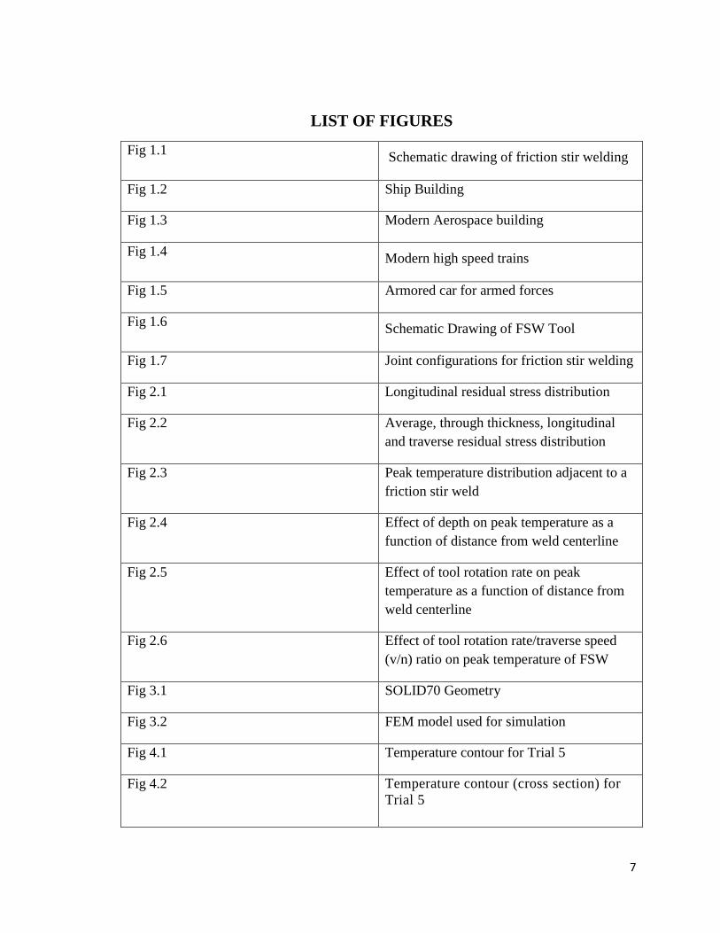
LIST OF FIGURES
Fig 1.1 Schematic drawing of friction stir welding
Fig 1.2 Ship Building
Fig 1.3 Modern Aerospace building
Fig 1.4 Modern high speed trains
Fig 1.5 Armored car for armed forces
Fig 1.6 Schematic Drawing of FSW Tool
Fig 1.7 Joint configurations for friction stir welding
Fig 2.1 Longitudinal residual stress distribution
Fig 2.2 Average, through thickness, longitudinal
and traverse residual stress distribution
Fig 2.3 Peak temperature distribution adjacent to a
friction stir weld
Fig 2.4 Effect of depth on peak temperature as a
function of distance from weld centerline
Fig 2.5 Effect of tool rotation rate on peak
temperature as a function of distance from
weld centerline
Fig 2.6 Effect of tool rotation rate/traverse speed
(v/n) ratio on peak temperature of FSW
Fig 3.1 SOLID70 Geometry
Fig 3.2 FEM model used for simulation
Fig 4.1 Temperature contour for Trial 5
Fig 4.2 Temperature contour (cross section) for
Trial 5

8
Fig 4.3 Effect of Welding speed on Maximum
temperature
Fig 4.4 Effect of Tool rotation speed on Maximum
temperature
Fig 4.5 Contour Plot of Temperature
Fig 4.6 Surface plot of temperature
Fig 4.7 Normal Probability plot of residual
Fig 4.8 Variation of Residual with run order

9
LIST OF TABLES
Table 2.1 Residual Stress measurements
Table 3.1 Thermal properties used for simulation
Table 4.1 Parameters used and temperatures
Table 4.2 t-test on Coefficients
Table 4.3 Parameters used and temperatures
10
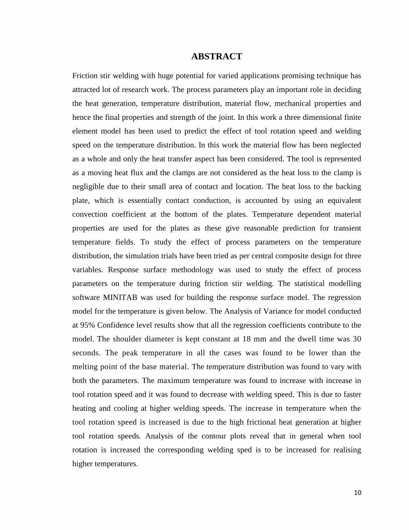
ABSTRACT
Friction stir welding with huge potential for varied applications promising technique has
attracted lot of research work. The process parameters play an important role in deciding
the heat generation, temperature distribution, material flow, mechanical properties and
hence the final properties and strength of the joint. In this work a three dimensional finite
element model has been used to predict the effect of tool rotation speed and welding
speed on the temperature distribution. In this work the material flow has been neglected
as a whole and only the heat transfer aspect has been considered. The tool is represented
as a moving heat flux and the clamps are not considered as the heat loss to the clamp is
negligible due to their small area of contact and location. The heat loss to the backing
plate, which is essentially contact conduction, is accounted by using an equivalent
convection coefficient at the bottom of the plates. Temperature dependent material
properties are used for the plates as these give reasonable prediction for transient
temperature fields. To study the effect of process parameters on the temperature
distribution, the simulation trials have been tried as per central composite design for three
variables. Response surface methodology was used to study the effect of process
parameters on the temperature during friction stir welding. The statistical modelling
software MINITAB was used for building the response surface model. The regression
model for the temperature is given below. The Analysis of Variance for model conducted
at 95% Confidence level results show that all the regression coefficients contribute to the
model. The shoulder diameter is kept constant at 18 mm and the dwell time was 30
seconds. The peak temperature in all the cases was found to be lower than the
melting point of the base material. The temperature distribution was found to vary with
both the parameters. The maximum temperature was found to increase with increase in
tool rotation speed and it was found to decrease with welding speed. This is due to faster
heating and cooling at higher welding speeds. The increase in temperature when the
tool rotation speed is increased is due to the high frictional heat generation at higher
tool rotation speeds. Analysis of the contour plots reveal that in general when tool
rotation is increased the corresponding welding sped is to be increased for realising
higher temperatures.
11
CHAPTER 1 Introduction
1.1 Friction Stir Welding
Friction stir welding (FSW) is a relatively innovative solid-state joining process. This
joining method is energy efficient, environment friendly, and versatile. In particular, it
can be used to join high-strength aerospace aluminum alloys and other metallic alloys
that are hard to weld by orthodox fusion welding. FSW is deemed to be the most
momentous development in metal joining in a decade. Recently, friction stir processing
(FSP) was developed for microstructural modification of metallic materials. In this
review article, the current state of understanding and development of the FSW and FSP
are addressed. Particular emphasis has been given to: (a) mechanisms responsible for the
formation of welds and microstructural refinement, and (b) effects of FSW/FSP
parameters on resultant microstructure and final mechanical properties. While the bulk of
the information is related to aluminum alloys important results are now available for
other metals and alloys. At this stage, the technology diffusion has significantly outpaced
the fundamental understanding of microstructural evolution and microstructure–property
relationships.
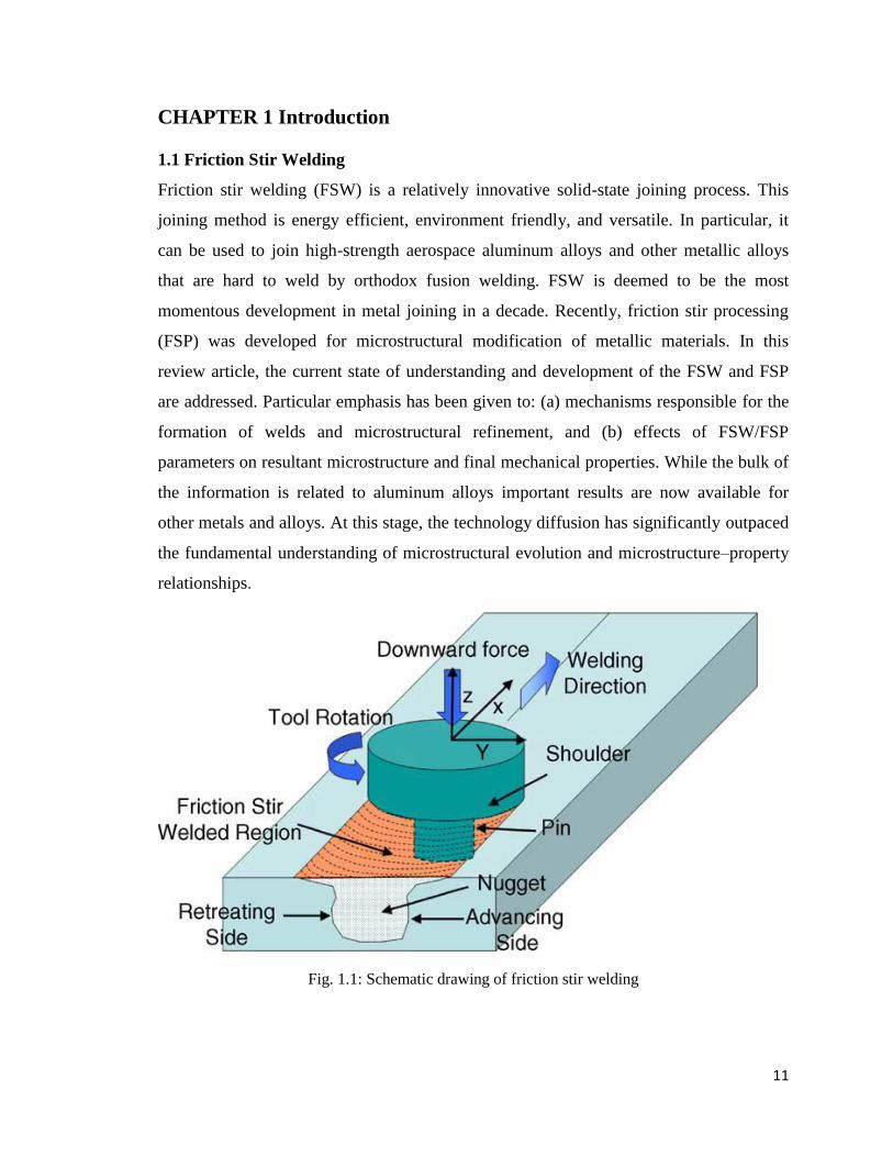
Fig. 1.1: Schematic drawing of friction stir welding
12
A constantly rotated non consumable cylindrical-shouldered tool with a profiled probe is
transversely fed at a constant rate into a butt joint between two clamped pieces of butted
material. The probe is slightly shorter than the weld depth required, with the tool shoulder
riding atop the work surface.
Frictional heat is generated between the wear-resistant welding components and the work
pieces. This heat, along with that generated by the mechanical mixing process and
the adiabatic heat within the material, cause the stirred materials to soften
without melting. As the pin is moved forward, a special profile on its leading face forces
plasticized material to the rear where clamping force assists in a forged consolidation of
the weld.
This process of the tool traversing along the weld line in a plasticized tubular shaft of
metal results in severe solid state deformation involving dynamic recrystallization of the
base material.
1.2 Advantages of FSW
FSW is considered to be the most significant development in metal joining in a decade
and is green technology due to its energy efficiency, environment friendliness, and
versatility. As compared to the conventional welding methods, FSW consumes
considerably less energy. No cover gas or flux is used, thereby making the process
environmentally friendly. The joining does not involve any use of filler metal and
therefore any aluminum alloy can be joined without concern for the compatibility of
composition, which is an issue in fusion welding. When desirable, dissimilar aluminum
alloys and composites can be joined with equal ease. In contrast to the traditional friction
welding, which is usually performed on small axisymmetric parts that can be rotated and
pushed against each other to form a joint, friction stir welding can be applied to various
types of joints like butt joints, lap joints, T butt joints, and fillet joints
1.3 Disadvantages of FSW
Exit hole left when tool is withdrawn. Large down forces are required with heavy-duty
fastening essential to grip the plates together. It is also less flexible than manual and arc
processes (difficulties with thickness variations and non-linear welds).Often slower
13
traverse rate than some fusion welding techniques, although this may be offset if fewer
welding passes are required.
1.4 Industrial Applications
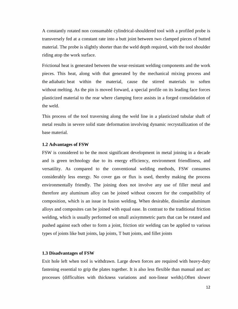
1.4.1 Shipbuilding and Marine Construction
The shipbuilding and marine industries are two of the first sectors that have adopted the
process for commercial applications.
The process is suitable for the following applications:
Panels for decks, sides, bulkheads and floors
Hulls and superstructures
Helicopter landing platforms
Marine and transport structures
Masts and booms, e.g. for sailing boats
Refrigeration plant
Fig 1.2: Ship Building
14
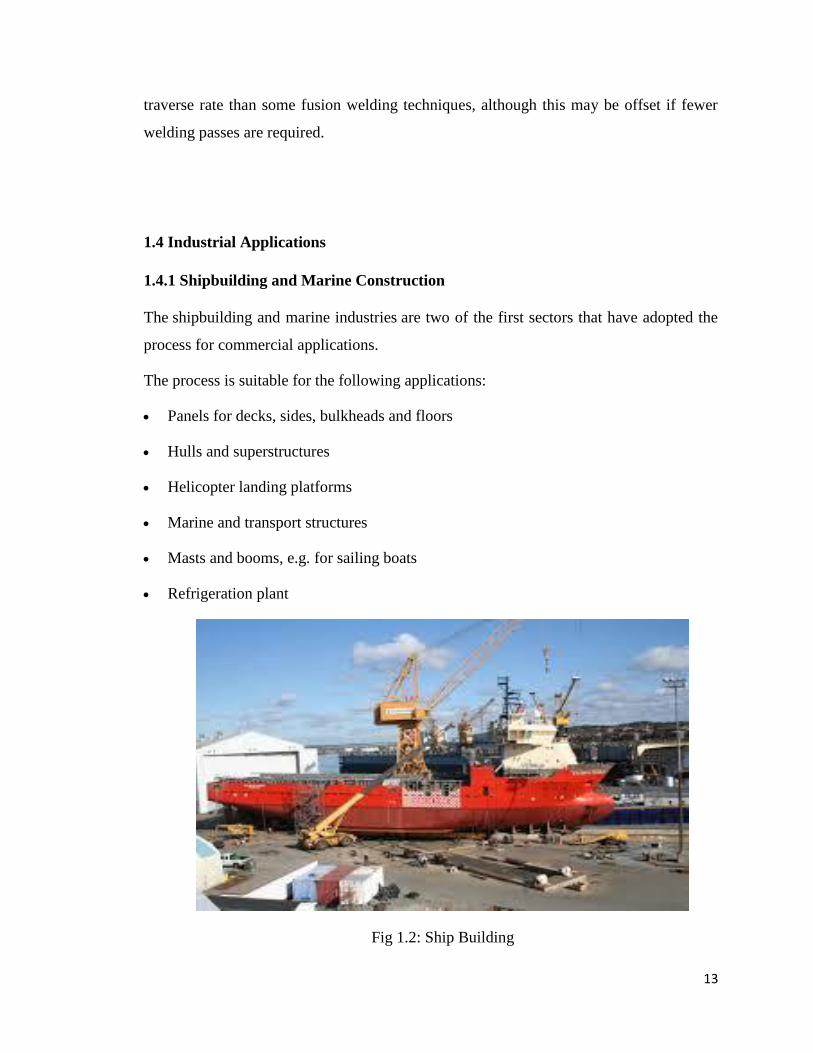
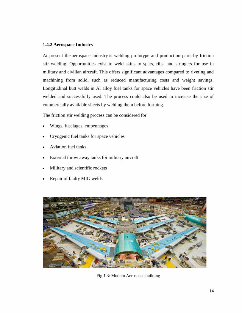
1.4.2 Aerospace Industry
At present the aerospace industry is welding prototype and production parts by friction
stir welding. Opportunities exist to weld skins to spars, ribs, and stringers for use in
military and civilian aircraft. This offers significant advantages compared to riveting and
machining from solid, such as reduced manufacturing costs and weight savings.
Longitudinal butt welds in Al alloy fuel tanks for space vehicles have been friction stir
welded and successfully used. The process could also be used to increase the size of
commercially available sheets by welding them before forming.
The friction stir welding process can be considered for:
Wings, fuselages, empennages
Cryogenic fuel tanks for space vehicles
Aviation fuel tanks
External throw away tanks for military aircraft
Military and scientific rockets
Repair of faulty MIG welds
Fig 1.3: Modern Aerospace building
15
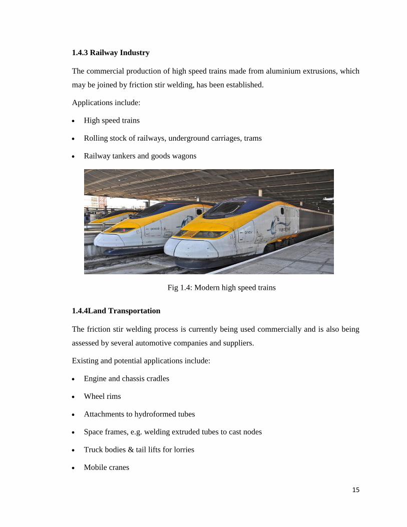
1.4.3 Railway Industry
The commercial production of high speed trains made from aluminium extrusions, which
may be joined by friction stir welding, has been established.
Applications include:
High speed trains
Rolling stock of railways, underground carriages, trams
Railway tankers and goods wagons
Fig 1.4: Modern high speed trains
1.4.4Land Transportation
The friction stir welding process is currently being used commercially and is also being
assessed by several automotive companies and suppliers.
Existing and potential applications include:
Engine and chassis cradles
Wheel rims
Attachments to hydroformed tubes
Space frames, e.g. welding extruded tubes to cast nodes
Truck bodies & tail lifts for lorries
Mobile cranes
16
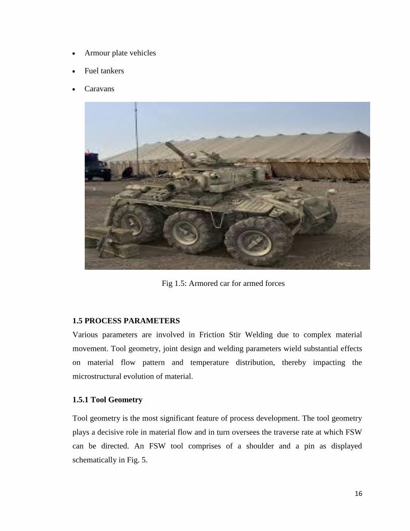
Armour plate vehicles
Fuel tankers
Caravans
Fig 1.5: Armored car for armed forces
1.5 PROCESS PARAMETERS
Various parameters are involved in Friction Stir Welding due to complex material
movement. Tool geometry, joint design and welding parameters wield substantial effects
on material flow pattern and temperature distribution, thereby impacting the
microstructural evolution of material.
1.5.1 Tool Geometry
Tool geometry is the most significant feature of process development. The tool geometry
plays a decisive role in material flow and in turn oversees the traverse rate at which FSW
can be directed. An FSW tool comprises of a shoulder and a pin as displayed
schematically in Fig. 5.
17
As mentioned prior, the tool has two major functions: (a) localized heating, and (b)
material flow. In the preliminary stage of tool plunge, the heating results predominantly
from the friction between pin and work piece. Further heating results from distortion of
material.
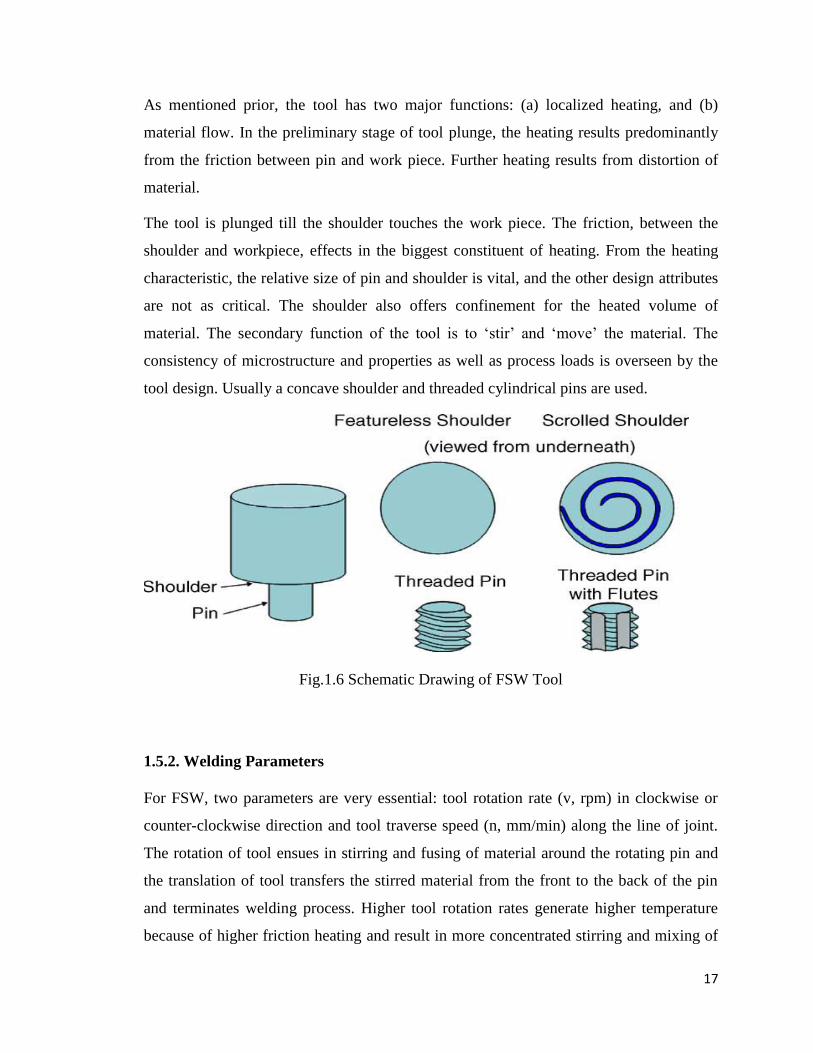
The tool is plunged till the shoulder touches the work piece. The friction, between the
shoulder and workpiece, effects in the biggest constituent of heating. From the heating
characteristic, the relative size of pin and shoulder is vital, and the other design attributes
are not as critical. The shoulder also offers confinement for the heated volume of
material. The secondary function of the tool is to ‘stir’ and ‘move’ the material. The
consistency of microstructure and properties as well as process loads is overseen by the
tool design. Usually a concave shoulder and threaded cylindrical pins are used.
Fig.1.6 Schematic Drawing of FSW Tool
1.5.2. Welding Parameters
For FSW, two parameters are very essential: tool rotation rate (v, rpm) in clockwise or
counter-clockwise direction and tool traverse speed (n, mm/min) along the line of joint.
The rotation of tool ensues in stirring and fusing of material around the rotating pin and
the translation of tool transfers the stirred material from the front to the back of the pin
and terminates welding process. Higher tool rotation rates generate higher temperature
because of higher friction heating and result in more concentrated stirring and mixing of
18
material as will be discussed later. However, it should be remarked that frictional
coupling of tool surface with workpiece is going to manage the heating. So, a monotonic
surge in heating with increasing tool rotation rate is not expected as the coefficient of
friction at interface will change with increasing tool rotation rate.
1.5.3 Joint Design
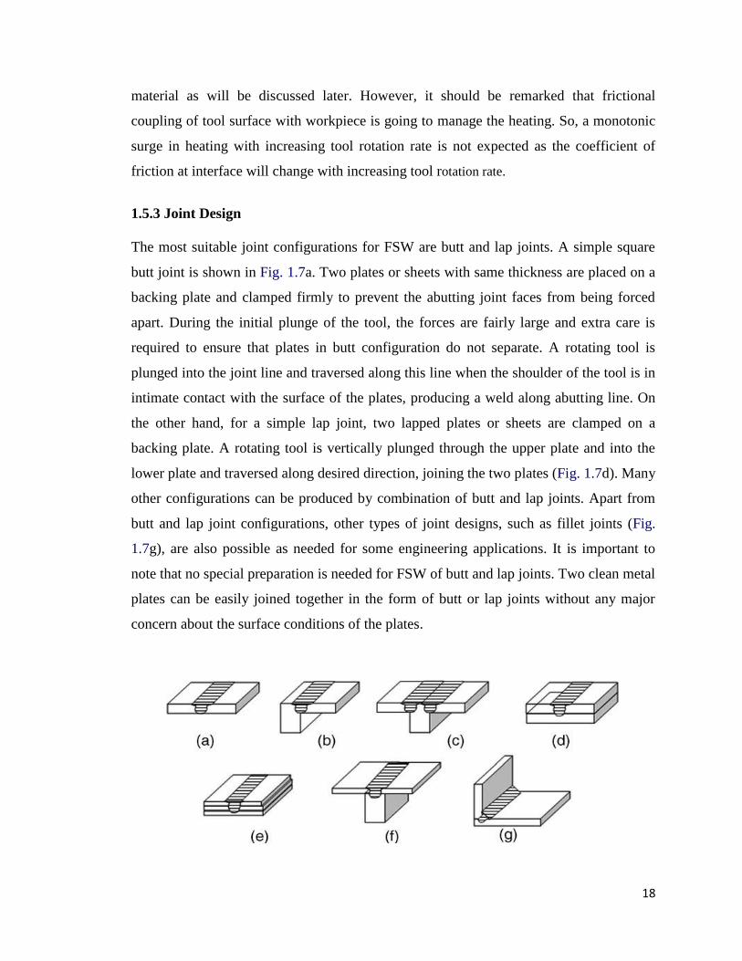
The most suitable joint configurations for FSW are butt and lap joints. A simple square
butt joint is shown in Fig. 1.7a. Two plates or sheets with same thickness are placed on a
backing plate and clamped firmly to prevent the abutting joint faces from being forced
apart. During the initial plunge of the tool, the forces are fairly large and extra care is
required to ensure that plates in butt configuration do not separate. A rotating tool is
plunged into the joint line and traversed along this line when the shoulder of the tool is in
intimate contact with the surface of the plates, producing a weld along abutting line. On
the other hand, for a simple lap joint, two lapped plates or sheets are clamped on a
backing plate. A rotating tool is vertically plunged through the upper plate and into the
lower plate and traversed along desired direction, joining the two plates (Fig. 1.7d). Many
other configurations can be produced by combination of butt and lap joints. Apart from
butt and lap joint configurations, other types of joint designs, such as fillet joints (Fig.
1.7g), are also possible as needed for some engineering applications. It is important to
note that no special preparation is needed for FSW of butt and lap joints. Two clean metal
plates can be easily joined together in the form of butt or lap joints without any major
concern about the surface conditions of the plates.
19
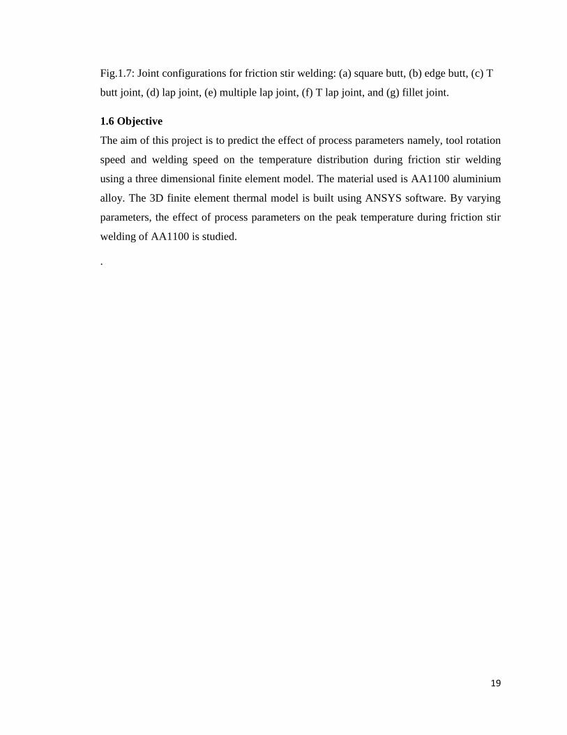
Fig.1.7: Joint configurations for friction stir welding: (a) square butt, (b) edge butt, (c) T
butt joint, (d) lap joint, (e) multiple lap joint, (f) T lap joint, and (g) fillet joint.
1.6 Objective
The aim of this project is to predict the effect of process parameters namely, tool rotation
speed and welding speed on the temperature distribution during friction stir welding
using a three dimensional finite element model. The material used is AA1100 aluminium
alloy. The 3D finite element thermal model is built using ANSYS software. By varying
parameters, the effect of process parameters on the peak temperature during friction stir
welding of AA1100 is studied.
.
20
CHAPTER 2: LITERATURE SURVEY
Initial attempts at thermal modelling of the FSW process were analytical in nature.
Subsequently, FEM based solid and thermal models and computational fluid dynamics
based viscoplastic flow models have replaced the analytical approach because of the
versatility of these methods. Although none of these efforts has combined all the aspects
of the modelling, namely, the flow visualisation, the material properties, and the thermal
profiles and histories, they have nevertheless contributed towards a greater understanding
of the process.
The earliest efforts on thermal modelling of friction stir welding started with the
Rosenthal equation for a uniformly moving point or line heat source to describe the heat
input. Russell and Shercliff adapted the existing analytical solutions for moving heat
sources and friction welding to model the friction stir welding by replacing the real heat
generation around the tool with equivalent simplified heat inputs such as the point source,
line source, and distributed surface heat input. McClure et al.presented some
experimental results accompanied with an intuitive analytical model similar to the
Rosenthal moving point source solution, and found that microstructures within the weld
zone are characterised by dynamic recrystallisation, grain growth, and complex aging
phenomena that show no evidence of melting.
They found that the maximum temperatures during the FSW process did not exceed
80%of the melting point temperature. They assumed that all the heat was generated by
the friction between the tool shoulder and the workpiece and considered only the
conduction mode of heat transfer. They also assumed that the downward pressure P
applied on the tool shoulder surface is uniform and correlated the heat generation rate
with the downward pressure using the friction coefficient. Using the analytical solution
for the Rosenthal moving point heat source and incorporating the frictional heat
generation as the heat source, they derived an integral equation to define the temperature
weld. In their model all thermo physical properties were assumed to be temperature
independent and the combined parameter µP (where µis the coefficient of friction and P
21
is the average uniform pressure at the tool shoulder) was fitted until the model predicted
the correct temperature at the centreline of the weld. They observed that a value of 5480
N (1230 lb) for µP resulted in a reasonable match between the experimental data and
simulated outputs at the weld centreline.
Gould and Feng and Feng et al. presented similar preliminary thermal models for FSW
that are analytical in nature and consider heat generation at the tool shoulder only. They
also used the Rosenthal equation to predict the quasi steady temperature weld due to a
moving point heat source of constant velocity and correlated the heat source with the
friction process at the shoulder.
Tang et al. investigated the heat input and temperature distribution during FSW and
found that the highest temperature in the weld seam was less than 80% of the melting
point for Al6061 – T6 and that, for the specific working conditions of 2 mm/s travel rate
and 300 – 1200 rev/min rotational speed, the temperature did not change appreciably in
the specimen thickness direction. They also observed that the temperature distribution
perpendicular to the weld was nearly isothermal under the tool shoulder, that the
temperature distribution is symmetric about the weld centerline and that increasing the
welding pressure and the rotational speed of the tool increased the peak welding
temperature.
They found an average thickness reduction of about 3% at the start of the weld and noted
that the shoulder of the pin tool played the most significant role in the welding process.
The microstructure of the welded joint showed that there was no melting during the
welding process. They found the grains at the weld centre to be fine and equiaxed
because of the large deformation that facilitates dynamic recrystallisation.
Chao and Qi presented a decoupled heat transfer model to study the temperature fields
developed during the FSW process. They used a FEM based three-dimensional model of
the thermal process in which it was assumed that all the heat was generated at the
frictional interface between the tool shoulder and the workpiece. The rate of heat input
was assumed to vary linearly with the radius of the tool shoulder and set directly
proportional to the coefficient of friction and the downward force exerted by the tool.
22
They considered the inner radius of the tool shoulder to be zero to compensate for the
heat generated by the tool pin.
In addition, they did not measure the downward force and consequently were obliged to
fit the combined variable µF(where F is the downward force) along with other estimated
variables. They used convection coefficient of 30 W m-2 K-1at the top surface of the
workpiece and modelled the bottom surface in contact with the backing plate with a
convective heat transfer coefficient determined by a trial and error procedure. They
determined that a convective coefficient of 500 Wm-2K-1correlated best with
experimental results.
Frigaard et al.used the finite difference technique to calculate the two- and three-
dimensional thermal fields during the FSW process and used these data in a separate
module to predict the resulting hardness distributions.
The model predictions of Frigaard et al. showed that the welding cycle has four major
stages: (i) the stationary heating period where the material beneath the shoulder is
preheated to a certain temperature (about 400°C for aluminium alloys) to allow the
plastic deformation during welding, (ii) the transient heating period during which heat
starts to build up around the shoulder as the tool starts to move, (iii) the pseudo-steady
state period where the thermal field around the tool remains essentially constant during
the welding operation, and (iv) the post-steady state period(with approximately three-
quarters of the weld completed)where the reflection of heat from the end plate surface
leads to additional buildup of heat around the tool shoulder and influences the heat
affected zone thermal profile.
They identified a process parameter q0 /vd(kJ mm-2) (where is q0 is the net power, v the
welding speed, and d the plate thickness) that controls the thermal behaviour during the
pseudo-steady state. They found that the heat source during the FSW is axisymmetric and
that the outer contour of the plastically deformed region corresponds approximately to the
450°C isotherm. They accounted for the heat generation due to plastic deformation by
using an elevated average value of the friction coefficient, m~0.4, which falls between
the values for sticky friction and dry sliding.
23
Colegrove et al. presented a finite element based thermal model of FSW that included the
backing plate and the tool and a flow model of the process that attempts to predict the
flow of material around the FSW tool. They used a pseudomaterial of reduced thermal
conductivity to simulate the contact between the aluminium and the steel backing plate.
However, they did not measure the power consumption during the FSW process and were
obliged to fit the heat input for overall agreement between modelled and measured
thermal cycles. They found that a shoulder heat input of 3474 W gave the best correlation
with the experimental data for the lower part of the weld. Khandkar and Khan presented a
friction based thermal model of overlap friction stir welding, whereas Khandkar and co-
workers presented some preliminary results on input torque based thermal modelling of
butt joining. In the friction based model of an overlap joint, they used a frictional heat
input at the tool shoulder–workpiece interface and used a value of 3% of the shoulder
flux for the regions that fall within the volume of the pin tool. They also incorporated the
effect of convective transport around the pin into the thermal model for overlap joints. In
an input torque based model of a butt joint, Khandkar et al. presented the novel idea of a
three-dimensional heat input model that emulates the shape of the pin tool in contact with
the workpiece by correlating the heat input with the experimentally measured input
torque.
This latter approach has been investigated and refined further in the present work. Smith
et al. presented the concept of a physics based model of the FSW process in which the
material close to the weld centreline is viewed as a highly viscous non-Newtonian fluid.
Seidel refined the idea further and implemented fluid dynamics based two-dimensional
and preliminary three dimensional models of the weld process. Seidel correlated the non-
Newtonian viscosity with the flow stress of the alloy through the Zener – Hollomon
parameter. The heat generated originates from the viscous dissipation of the laminar flow.
None of the above mentioned works, except those of Khandkar and Khan and Khandkar
et al. incorporated a truly three-dimensional heat source along with the backing plate
attached to the bottom surface of the workpiece offering a thermal contact resistance in
between.
24
Although Colegrove et al made such an attempt, it was necessary to fit their heat input
values to match the experimentally determined temperature data. In the present work, a
heat input model that approximates the contour of the profiled tool by correlating the heat
source with the input torque has been explored.
This model is a distinct improvement over previous frictional heating models in which it
was necessary to rely on inverse estimation of the frictional coefficient for compliance
between the modeled heat source and the temperature data. Parametric analyses have also
been presented to study the effects on the thermal profiles of (i) different heat transfer
conditions at the bottom of the workpiece, (ii) backing plates of different material
(different conductivities), and (iii) different contact gap conductances at the workpiece –
backing plate interface.
2.2 Residual Stress
During fusion welding, complex thermal and mechanical stresses develop in the weld and
surrounding region due to the localized application of heat and accompanying constraint.
Following fusion welding, residual stresses commonly approach the yield strength of the
base material. It is generally believed that residual stresses are low in friction stir welds
due to low temperature solid-state process of FSW. However, compared to more
compliant clamps used for fixing the parts in conventional welding processes, the rigid
clamping used in FSW exerts a much higher restraint on the welded plates. These
restraints impede the contraction of the weld nugget and heat-affected zone during
cooling in both longitudinal and transverse directions, thereby resulting in generation of
longitudinal and transverse stresses. The existence of high value of residual stress exerts a
significant effect on the post-weld mechanical properties, particularly the fatigue
properties. Therefore, it is of practical importance to investigate the residual stress
distribution in the FSW welds. James and Mahoney measured residual stress in the FSW
7050Al-T7451, C458 Al–Li alloy, and 2219Al by means of X-ray diffraction sin2 c
method. Typical results obtained in FSW 7050Al- T7451 by pinhole X-ray beam (1 mm)
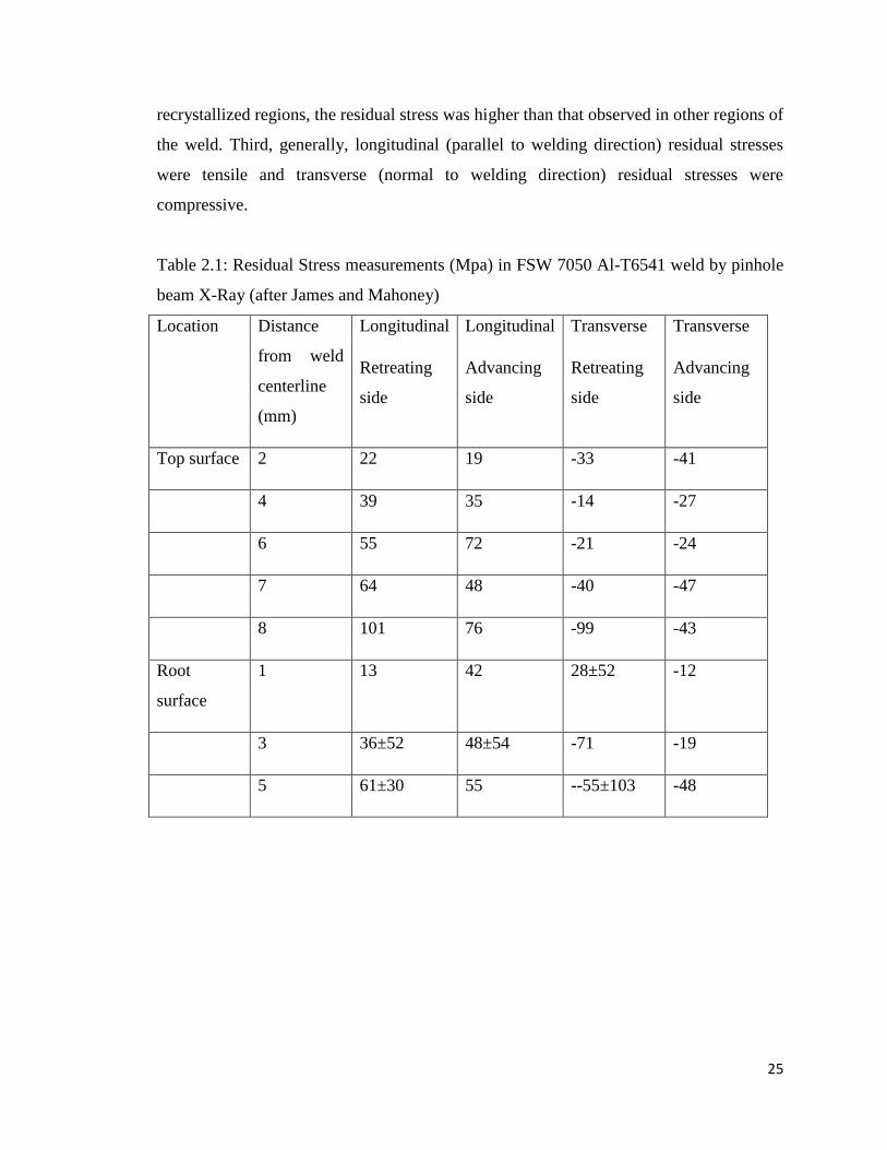
are tabulated in Table 1. This investigation revealed following findings. First, the residual
stresses in all the FSW welds were quite low compared to those generated during fusion
welding. Second, at the transition between the fully recrystallized and partially
25
recrystallized regions, the residual stress was higher than that observed in other regions of
the weld. Third, generally, longitudinal (parallel to welding direction) residual stresses
were tensile and transverse (normal to welding direction) residual stresses were
compressive.
Table 2.1: Residual Stress measurements (Mpa) in FSW 7050 Al-T6541 weld by pinhole
beam X-Ray (after James and Mahoney)
Location Distance
from weld
centerline
(mm)
Longitudinal
Retreating
side
Longitudinal
Advancing
side
Transverse
Retreating
side
Transverse
Advancing
side
Top surface 2 22 19 -33 -41
4 39 35 -14 -27
6 55 72 -21 -24
7 64 48 -40 -47
8 101 76 -99 -43
Root
surface
1 13 42 28±52 -12
3 36±52 48±54 -71 -19
5 61±30 55 --55±103 -48
26
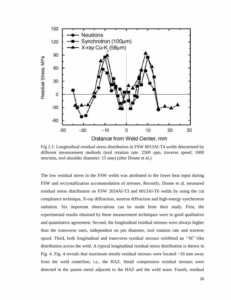
Fig 2.1: Longitudinal residual stress distribution in FSW 6013Al-T4 welds determined by
different measurement methods (tool rotation rate: 2500 rpm, traverse speed: 1000
mm/min, tool shoulder diameter: 15 mm) (after Donne et al.)
The low residual stress in the FSW welds was attributed to the lower heat input during
FSW and recrystallization accommodation of stresses. Recently, Donne et al. measured
residual stress distribution on FSW 2024Al-T3 and 6013Al-T6 welds by using the cut
compliance technique, X-ray diffraction, neutron diffraction and high-energy synchrotron
radiation. Six important observations can be made from their study. First, the
experimental results obtained by these measurement techniques were in good qualitative
and quantitative agreement. Second, the longitudinal residual stresses were always higher
than the transverse ones, independent on pin diameter, tool rotation rate and traverse
speed. Third, both longitudinal and transverse residual stresses exhibited an ‘‘M’’-like
distribution across the weld. A typical longitudinal residual stress distribution is shown in
Fig. 4. Fig. 4 reveals that maximum tensile residual stresses were located ~10 mm away
from the weld centerline, i.e., the HAZ. Small compressive residual stresses were
detected in the parent metal adjacent to the HAZ and the weld seam. Fourth, residual
27
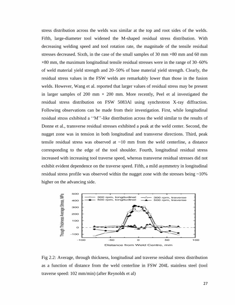
stress distribution across the welds was similar at the top and root sides of the welds.
Fifth, large-diameter tool widened the M-shaped residual stress distribution. With
decreasing welding speed and tool rotation rate, the magnitude of the tensile residual
stresses decreased. Sixth, in the case of the small samples of 30 mm ×80 mm and 60 mm
×80 mm, the maximum longitudinal tensile residual stresses were in the range of 30–60%
of weld material yield strength and 20–50% of base material yield strength. Clearly, the
residual stress values in the FSW welds are remarkably lower than those in the fusion
welds. However, Wang et al. reported that larger values of residual stress may be present
in larger samples of 200 mm × 200 mm. More recently, Peel et al investigated the
residual stress distribution on FSW 5083Al using synchrotron X-ray diffraction.
Following observations can be made from their investigation. First, while longitudinal
residual stress exhibited a ‘‘M’’-like distribution across the weld similar to the results of
Donne et al., transverse residual stresses exhibited a peak at the weld center. Second, the
nugget zone was in tension in both longitudinal and transverse directions. Third, peak
tensile residual stress was observed at ~10 mm from the weld centerline, a distance
corresponding to the edge of the tool shoulder. Fourth, longitudinal residual stress
increased with increasing tool traverse speed, whereas transverse residual stresses did not
exhibit evident dependence on the traverse speed. Fifth, a mild asymmetry in longitudinal
residual stress profile was observed within the nugget zone with the stresses being ~10%
higher on the advancing side.
Fig 2.2: Average, through thickness, longitudinal and traverse residual stress distribution
as a function of distance from the weld centerline in FSW 204L stainless steel (tool
traverse speed: 102 mm/min) (after Reynolds et al)
28
Sixth, similar to the results of Donne et al., maximum residual stresses in longitudinal
direction (40–60 MPa) were higher than that in transverse direction (20–40 MPa).Clearly,
maximum residual stresses observed in various friction stir welds of aluminum alloys
were below 100 MPa. The residual stress magnitudes are significantly lower than those
observed in fusion welding, and also significantly lower than yield stress of these
aluminum alloys. This results in a significant reduction in the distortion of FSW
components and an improvement in mechanical properties. On the other hand, Reynolds
et al.measured residual stress of 304L stainless steel FSW welds by neutron diffraction.
Average through thickness, longitudinal and transverse residual stresses are presented in
Fig. 2.2 as a function of distance from the weld centerline. Fig. 2.2 revealed the following
observations. First, the residual stress patterns observed for FSW are typical of most
welding processes such as fusion welding, namely, high value of longitudinal tensile
residual stress and very low transverse residual stress. Second, the maximum values of
longitudinal residual stress were close to the base metal yield stress, and therefore similar
in magnitude to those produced by fusion welding processes in austenitic stainless steels.
Third, increasing tool rotation rate from 300 to 500 rpm at a constant tool traverse speed
of 102 mm/min did not exert marked effect on the residual stress distribution apart from
slightly widening the range of high values of residual stress. Further, Reynolds et
al.reported that the longitudinal residual stress varied only slightly with depth, whereas
the transverse stress varied significantly through the thickness. The sign of the transverse
residual stress near the weld centerline was in general positive at the crown and negative
at the root. This was attributed to rapid cooling experienced by the weld root due to the
intimate contact between the weld root side and the backing plate. Clearly, the
distribution and magnitude of residual stress in friction stir welds are different for
aluminum alloy and steel. This is likely to be related to the temperature dependence of
the yield strength and the influence of final deformation by the trailing edge of the tool
shoulder.
2.3 Temperature Distribution
FSW results in intense plastic deformation around rotating tool and friction between tool
and workpieces. Both these factors contribute to the temperature increase within and
around the stirred zone. Since the temperature distribution within and around the stirred
29
zone directly influences the microstructure of the welds, such as grain size, grain
boundary character, coarsening and dissolution of precipitates, and resultant mechanical
properties of the welds, it is important to obtain information about temperature
distribution during FSW. However, temperature measurements within the stirred zone are
very difficult due to the intense plastic deformation produced by the rotation and
translation of tool. Therefore, the maximum temperatures within the stirred zone during
FSW have been either estimated from the microstructure of the weld or recorded by
embedding thermocouple in the regions adjacent to the rotating pin. An investigation of
microstructural evolution in 7075Al-T651 during FSW by Rhodes et al. showed
dissolution of larger precipitates and reprecipitation in the weld center. Therefore, they
concluded that maximum process temperatures are between about 400 and 480 8C in an
FSW 7075Al- T651. On the hand, Murr and co-workers indicated that some of the
precipitates were not dissolved during welding and suggested that the temperature rises to
roughly 400 8C in an FSW 6061Al. Recently, Sato et al.studied the microstructural
evolution of 6063Al during FSW using transmission electron microscopy (TEM) and
compared it with that of simulated weld thermal cycles. They reported that the
precipitates within the weld region (0–8.5 mm from weld center) were completely
dissolved into aluminum matrix. By comparing with the microstructures of simulated
weld thermal cycles at different peak temperatures, they concluded that the regions 0–8.5,
10, 12.5, and 15 mm away from the friction stir weld center were heated to temperatures
higher than 402, 353, 302 ºC and lower than 201 ºC, respectively. Recently, Mahoney et
al. conducted friction stir welding of 6.35 mm thick 7075Al-T651 plate and measured the
temperature distribution around the stirred zone both as a function of distance from the
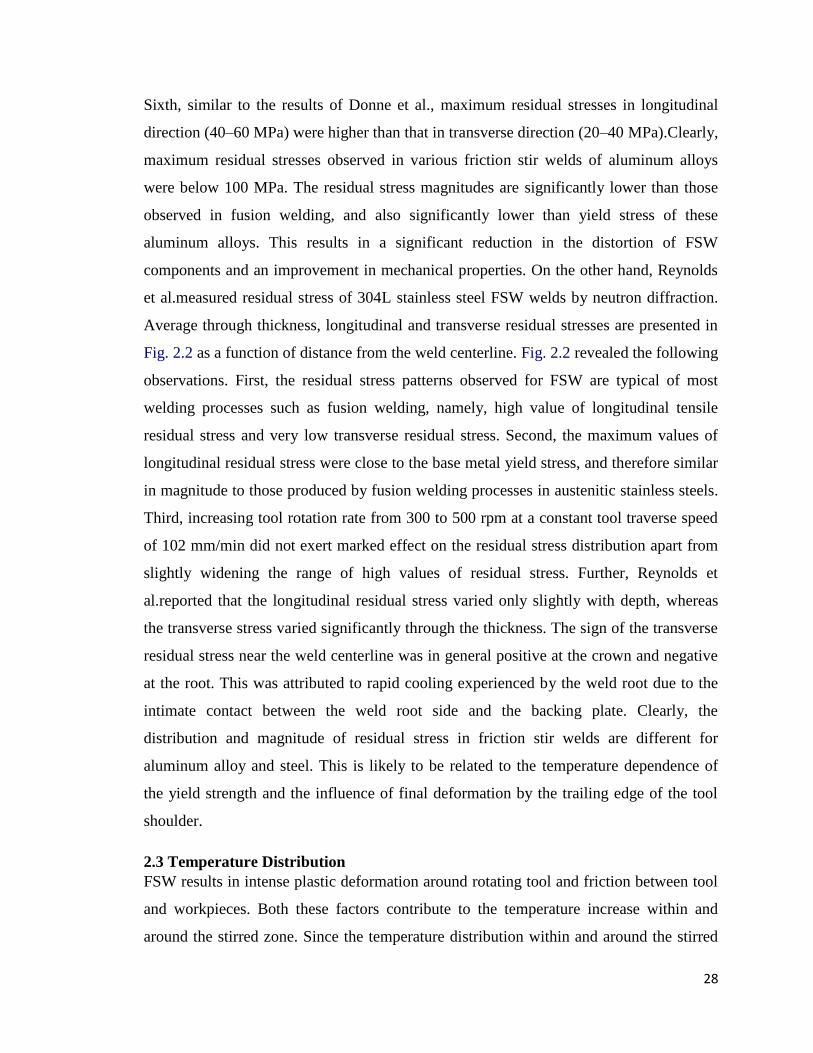
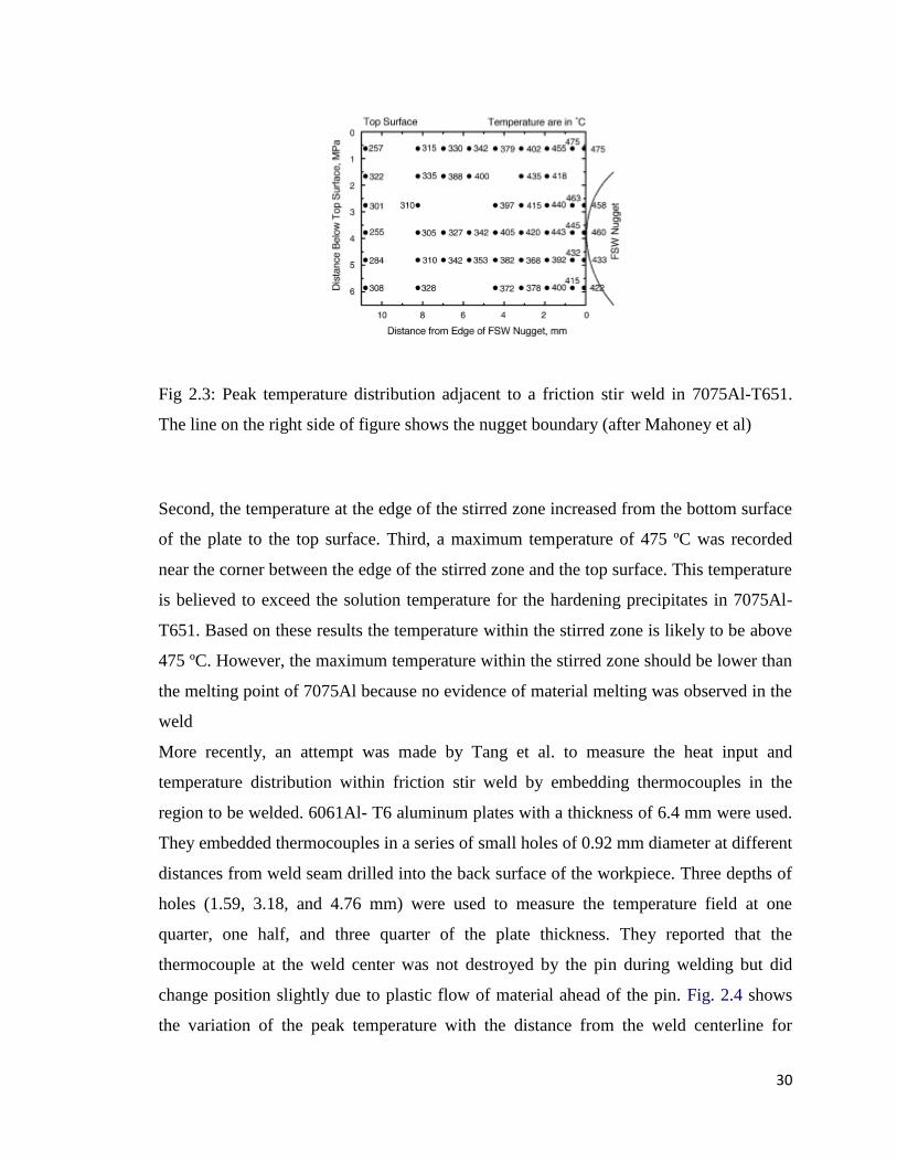
stirred zone and through the thickness of the sheet. Fig. 2.3 shows the peak temperature
distribution adjacent to the stirred zone. Fig.2.3 reveals three important observations.
First, maximum temperature was recorded at the locations close to the stirred zone, i.e.,
the edge of the stirred zone, and the temperature decreased with increasing distance from
the stirred zone.
30
Fig 2.3: Peak temperature distribution adjacent to a friction stir weld in 7075Al-T651.
The line on the right side of figure shows the nugget boundary (after Mahoney et al)
Second, the temperature at the edge of the stirred zone increased from the bottom surface
of the plate to the top surface. Third, a maximum temperature of 475 ºC was recorded
near the corner between the edge of the stirred zone and the top surface. This temperature
is believed to exceed the solution temperature for the hardening precipitates in 7075Al-
T651. Based on these results the temperature within the stirred zone is likely to be above
475 ºC. However, the maximum temperature within the stirred zone should be lower than
the melting point of 7075Al because no evidence of material melting was observed in the
weld
More recently, an attempt was made by Tang et al. to measure the heat input and
temperature distribution within friction stir weld by embedding thermocouples in the
region to be welded. 6061Al- T6 aluminum plates with a thickness of 6.4 mm were used.
They embedded thermocouples in a series of small holes of 0.92 mm diameter at different
distances from weld seam drilled into the back surface of the workpiece. Three depths of
holes (1.59, 3.18, and 4.76 mm) were used to measure the temperature field at one
quarter, one half, and three quarter of the plate thickness. They reported that the
thermocouple at the weld center was not destroyed by the pin during welding but did
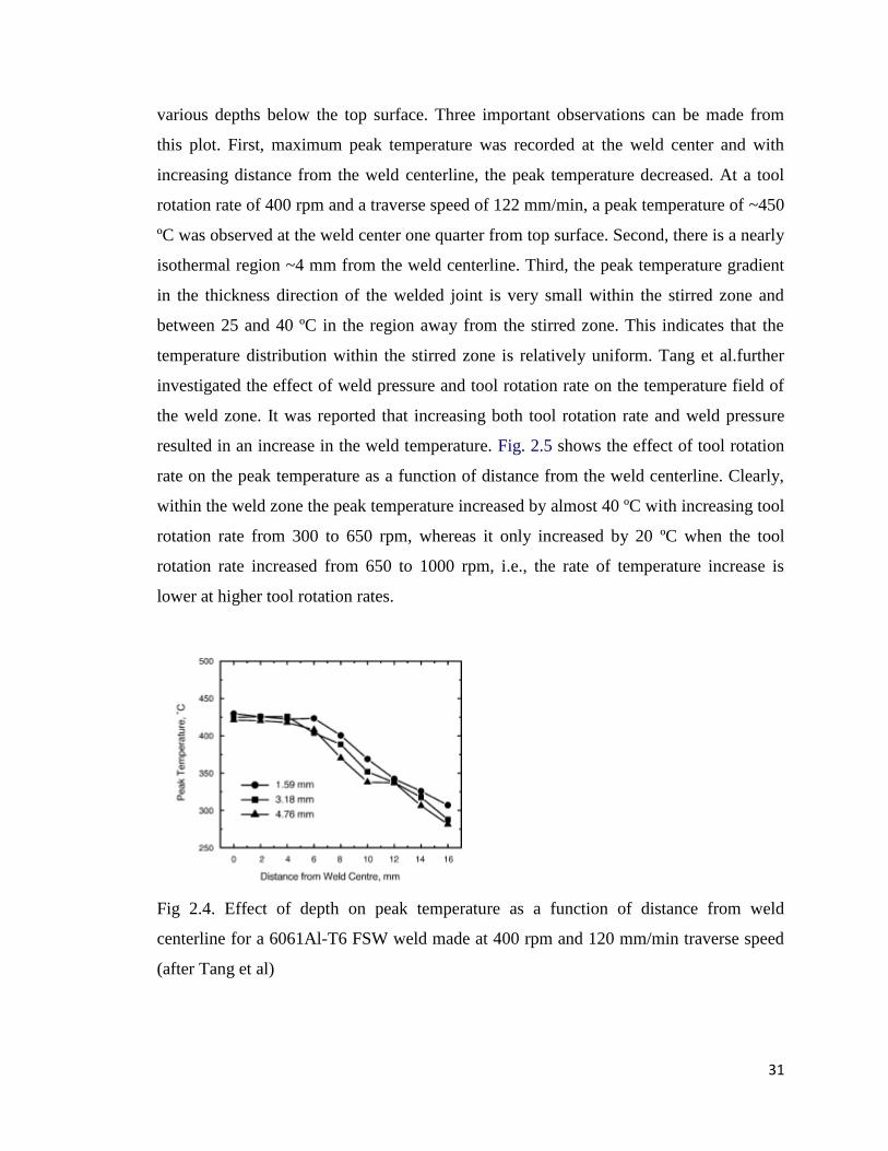
change position slightly due to plastic flow of material ahead of the pin. Fig. 2.4 shows
the variation of the peak temperature with the distance from the weld centerline for
31
various depths below the top surface. Three important observations can be made from
this plot. First, maximum peak temperature was recorded at the weld center and with
increasing distance from the weld centerline, the peak temperature decreased. At a tool
rotation rate of 400 rpm and a traverse speed of 122 mm/min, a peak temperature of ~450
ºC was observed at the weld center one quarter from top surface. Second, there is a nearly
isothermal region ~4 mm from the weld centerline. Third, the peak temperature gradient
in the thickness direction of the welded joint is very small within the stirred zone and
between 25 and 40 ºC in the region away from the stirred zone. This indicates that the
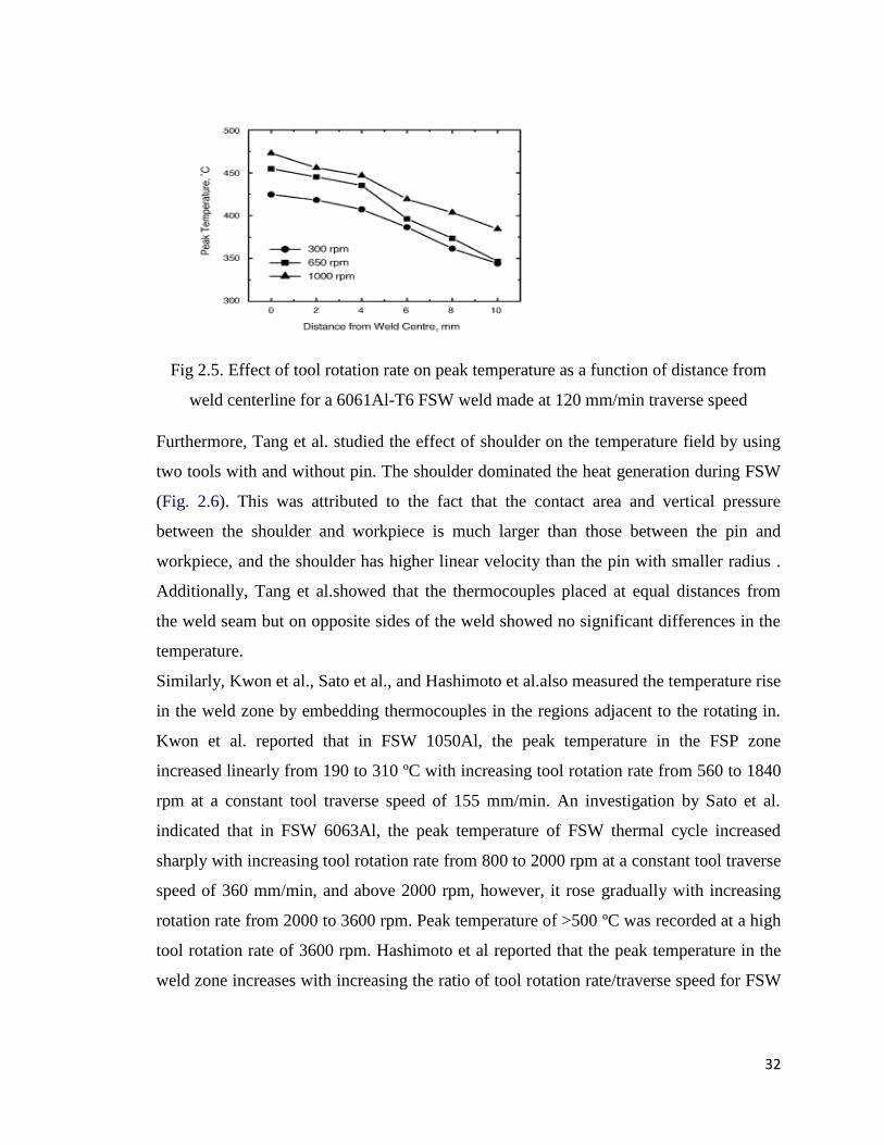
temperature distribution within the stirred zone is relatively uniform. Tang et al.further
investigated the effect of weld pressure and tool rotation rate on the temperature field of
the weld zone. It was reported that increasing both tool rotation rate and weld pressure
resulted in an increase in the weld temperature. Fig. 2.5 shows the effect of tool rotation
rate on the peak temperature as a function of distance from the weld centerline. Clearly,
within the weld zone the peak temperature increased by almost 40 ºC with increasing tool
rotation rate from 300 to 650 rpm, whereas it only increased by 20 ºC when the tool
rotation rate increased from 650 to 1000 rpm, i.e., the rate of temperature increase is
lower at higher tool rotation rates.
Fig 2.4. Effect of depth on peak temperature as a function of distance from weld
centerline for a 6061Al-T6 FSW weld made at 400 rpm and 120 mm/min traverse speed
(after Tang et al)
32
Fig 2.5. Effect of tool rotation rate on peak temperature as a function of distance from
weld centerline for a 6061Al-T6 FSW weld made at 120 mm/min traverse speed
Furthermore, Tang et al. studied the effect of shoulder on the temperature field by using
two tools with and without pin. The shoulder dominated the heat generation during FSW
(Fig. 2.6). This was attributed to the fact that the contact area and vertical pressure
between the shoulder and workpiece is much larger than those between the pin and
workpiece, and the shoulder has higher linear velocity than the pin with smaller radius .
Additionally, Tang et al.showed that the thermocouples placed at equal distances from
the weld seam but on opposite sides of the weld showed no significant differences in the
temperature.
Similarly, Kwon et al., Sato et al., and Hashimoto et al.also measured the temperature rise
in the weld zone by embedding thermocouples in the regions adjacent to the rotating in.
Kwon et al. reported that in FSW 1050Al, the peak temperature in the FSP zone
increased linearly from 190 to 310 ºC with increasing tool rotation rate from 560 to 1840
rpm at a constant tool traverse speed of 155 mm/min. An investigation by Sato et al.
indicated that in FSW 6063Al, the peak temperature of FSW thermal cycle increased
sharply with increasing tool rotation rate from 800 to 2000 rpm at a constant tool traverse
speed of 360 mm/min, and above 2000 rpm, however, it rose gradually with increasing
rotation rate from 2000 to 3600 rpm. Peak temperature of >500 ºC was recorded at a high
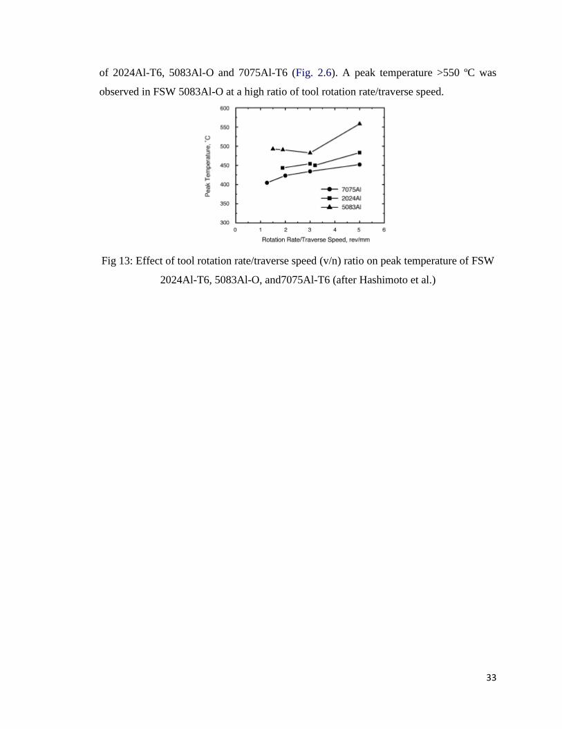
tool rotation rate of 3600 rpm. Hashimoto et al reported that the peak temperature in the
weld zone increases with increasing the ratio of tool rotation rate/traverse speed for FSW
33
of 2024Al-T6, 5083Al-O and 7075Al-T6 (Fig. 2.6). A peak temperature >550 ºC was
observed in FSW 5083Al-O at a high ratio of tool rotation rate/traverse speed.
Fig 13: Effect of tool rotation rate/traverse speed (v/n) ratio on peak temperature of FSW
2024Al-T6, 5083Al-O, and7075Al-T6 (after Hashimoto et al.)
34
CHAPTER 3 MODELLING OF FSW IN ANSYS
3.1 Introduction
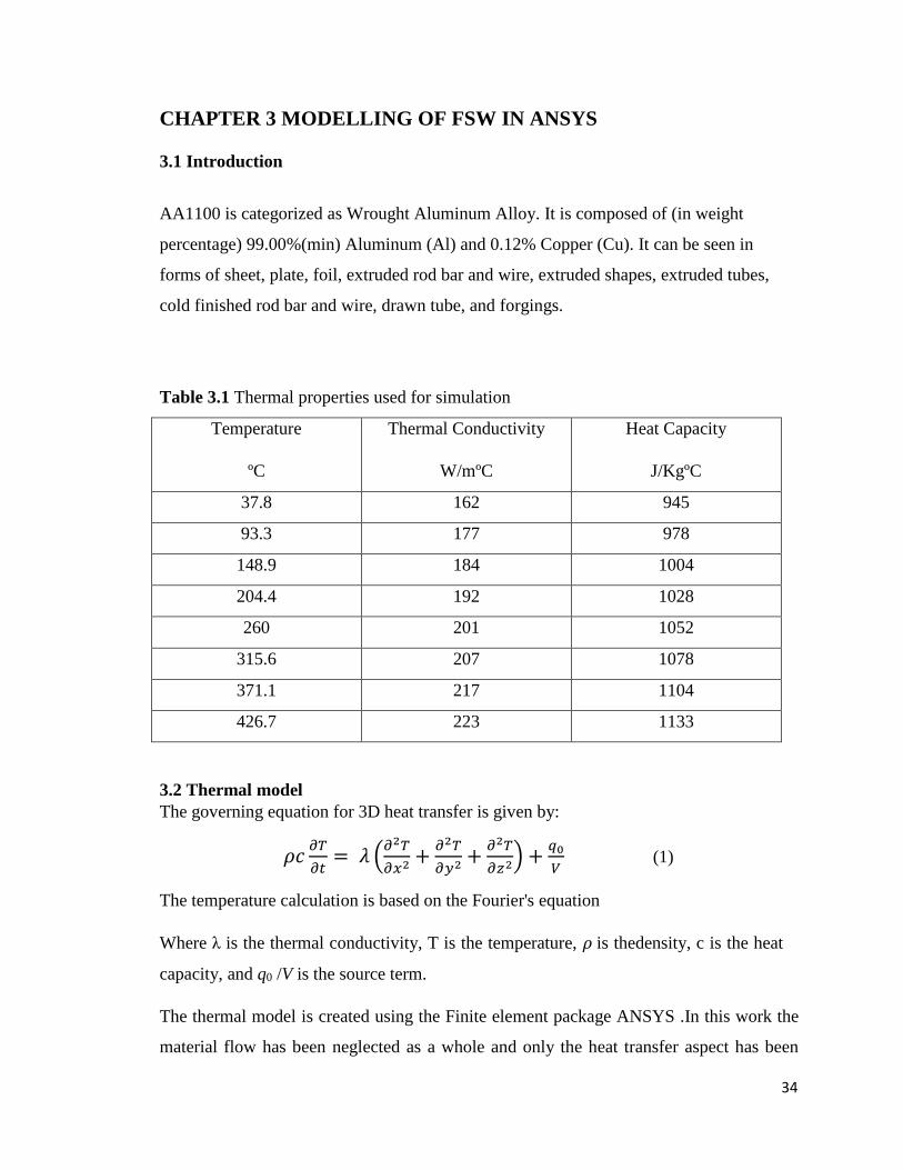
AA1100 is categorized as Wrought Aluminum Alloy. It is composed of (in weight
percentage) 99.00%(min) Aluminum (Al) and 0.12% Copper (Cu). It can be seen in
forms of sheet, plate, foil, extruded rod bar and wire, extruded shapes, extruded tubes,
cold finished rod bar and wire, drawn tube, and forgings.
Table 3.1 Thermal properties used for simulation
Temperature
ºC
Thermal Conductivity
W/mºC
Heat Capacity
J/KgºC
37.8 162 945
93.3 177 978
148.9 184 1004
204.4 192 1028
260 201 1052
315.6 207 1078
371.1 217 1104
426.7 223 1133
3.2 Thermal model
The governing equation for 3D heat transfer is given by:
𝜌𝑐𝜕𝑇
𝜕𝑡= 𝜆 (
𝜕2𝑇
𝜕𝑥2+
𝜕2𝑇
𝜕𝑦2+
𝜕2𝑇
𝜕𝑧2) +𝑞0
𝑉 (1)
The temperature calculation is based on the Fourier's equation
Where λ is the thermal conductivity, T is the temperature, 𝜌 is thedensity, c is the heat
capacity, and q0 /V is the source term.
The thermal model is created using the Finite element package ANSYS .In this work the
material flow has been neglected as a whole and only the heat transfer aspect has been
35
considered. The tool is represented as a moving heat flux and the clamps are not
considered as the heat loss to the clamp is negligible due to their small area of contact and
location. The plates are represented by a finite element mesh of 8 node thermal brick
elements with temperature as the only degree of freedom. To reduce the computational
requirements, regions around the weld line are meshed with smaller element, while the
element size farther from the weld line is larger. The heat loss into the tool is accounted
by reducing the energy input into the plate. Convection coefficient for all the surfaces
exposed to atmosphere is 30 W/m2 K. The heat loss to the backing plate, which is
essentially contact conduction, is accounted by using an equivalent convection coefficient
at the bottom of the plates. Constant room-temperature properties are used for the plates
as these give reasonable prediction for transient temperature fields.
3.4 Heat Generation
In FSW, heat is generated due to friction and plastic deformation at the tool workpiece
interface and at the TMAZ. The heat generation at the contact surfaces due to friction is
the product of frictional force and the tangential speed of the tool with respect to the
workpiece. The heat generated per unit area due to plastic deformation at the tool-
workpiece interface is the product of shear stress and the velocity of the workpiece
material sticking to the tool as it traverses. This velocity is actually the tangential speed
of the tool. The heat generation due to friction on an elemental area dA at the tool-
workpiece interface, considering high rotational speed compared to traverse speed of the
FSW tool, is given by:
𝑑𝑄𝑓 = (1 − 𝛿)𝜔𝑟𝜇𝑝𝑑A (2)
The heat generated due to plastic shear deformation leading to workpiece material
sticking to the tool is given by:
𝑑𝑄𝑝 = 𝛿𝜔𝑟𝜏𝑦𝑑𝐴 (3)
Therefore, total heat due to friction and plastic deformation is given by:
𝑑𝑄 = 𝑑𝑄𝑓 + 𝑑𝑄𝑝 = 𝜔𝑟𝑑𝐴(𝜇𝑝 − 𝛿𝜇𝑝) + 𝛿𝜏𝑦 (4)
36
Let 𝜏𝑐𝑜𝑛𝑡𝑎𝑐𝑡 = [(𝜇𝑝 − 𝛿𝜇𝑝) + 𝛿𝜏𝑦 (5)
Therefore, 𝑑𝑄 = 𝜔𝑟𝑑𝐴𝜏𝑐𝑜𝑛𝑡𝑎𝑐𝑡 (6)
There is no straightforward mechanism to estimate the extent of slip. At the same time,
with the increase in temperature, the yield strength of the workpiece material decreases,
resulting in reduction in heat generation from plastic deformation. In such a situation, it
was felt more logical to consider pure friction and neglect the heat generation due to
plastic deformation. In the case of pure friction δ = 0. Therefore,
Equation 16 reduces to:
𝜏𝑐𝑜𝑛𝑡𝑎𝑐𝑡 = 𝜇𝑝 (7)
Therefore, from Equations 17 and 18, the expression for heat generation on an elemental
surface area dA at the tool-workpiece interface is given by:
𝑑𝑄 = 𝜔𝑟𝜇𝑝 𝑑𝐴 (8)
i.e.,𝑑𝑄 = 𝜔𝑟 𝑑𝐹 (9)
where 𝑑𝐹 = 𝜇𝑝 𝑑𝐴 (10)
The three distinct tool-workpiece interface surfaces are tool shoulder, tool pin side, and
tool pin tip. However, the contribution of tool tip surface is negligible toward the total
heat generation required for welding. Q1 and Q2 are the components of the respective heat
generated from the tool shoulder and tool pin side interfaces. Therefore, the total heat
generated is given by Qtotal = Q1 + Q2 .
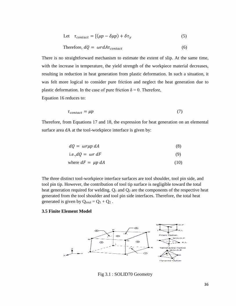
3.5 Finite Element Model
Fig 3.1 : SOLID70 Geometry
37
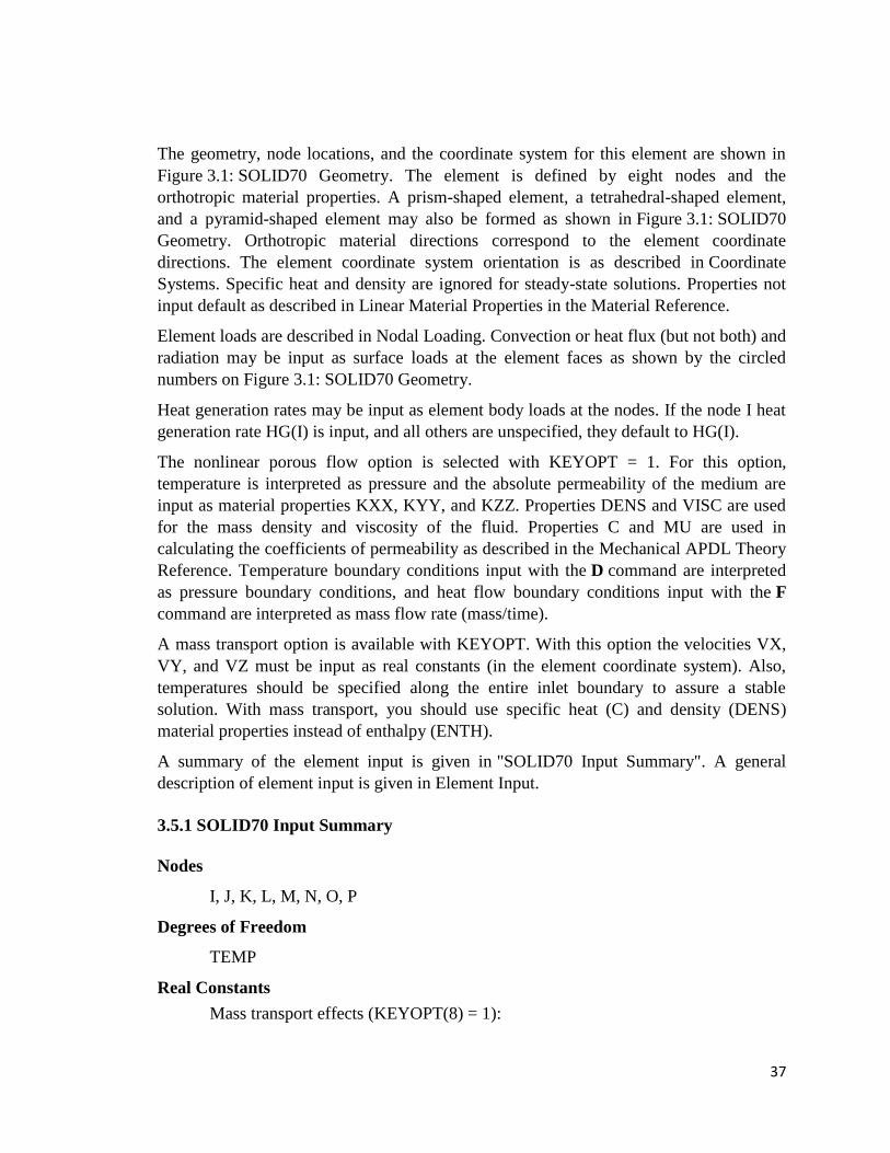
The geometry, node locations, and the coordinate system for this element are shown in
Figure 3.1: SOLID70 Geometry. The element is defined by eight nodes and the
orthotropic material properties. A prism-shaped element, a tetrahedral-shaped element,
and a pyramid-shaped element may also be formed as shown in Figure 3.1: SOLID70
Geometry. Orthotropic material directions correspond to the element coordinate
directions. The element coordinate system orientation is as described in Coordinate
Systems. Specific heat and density are ignored for steady-state solutions. Properties not
input default as described in Linear Material Properties in the Material Reference.
Element loads are described in Nodal Loading. Convection or heat flux (but not both) and
radiation may be input as surface loads at the element faces as shown by the circled
numbers on Figure 3.1: SOLID70 Geometry.
Heat generation rates may be input as element body loads at the nodes. If the node I heat
generation rate HG(I) is input, and all others are unspecified, they default to HG(I).
The nonlinear porous flow option is selected with KEYOPT = 1. For this option,
temperature is interpreted as pressure and the absolute permeability of the medium are
input as material properties KXX, KYY, and KZZ. Properties DENS and VISC are used
for the mass density and viscosity of the fluid. Properties C and MU are used in
calculating the coefficients of permeability as described in the Mechanical APDL Theory
Reference. Temperature boundary conditions input with the D command are interpreted
as pressure boundary conditions, and heat flow boundary conditions input with the F
command are interpreted as mass flow rate (mass/time).
A mass transport option is available with KEYOPT. With this option the velocities VX,
VY, and VZ must be input as real constants (in the element coordinate system). Also,
temperatures should be specified along the entire inlet boundary to assure a stable
solution. With mass transport, you should use specific heat (C) and density (DENS)
material properties instead of enthalpy (ENTH).
A summary of the element input is given in "SOLID70 Input Summary". A general
description of element input is given in Element Input.
3.5.1 SOLID70 Input Summary
Nodes
I, J, K, L, M, N, O, P
Degrees of Freedom
TEMP
Real Constants
Mass transport effects (KEYOPT(8) = 1):
38
VX - X direction of mass transport velocity
VY - Y direction of mass transport velocity
VZ - Z direction of mass transport velocity
Material Properties
MP command: KXX, KYY, KZZ, DENS, C, ENTH, VISC, MU (VISC and MU
used only if KEYOPT = 1.
Do not use ENTH with KEYOPT = 1.
Surface Loads
Convection or Heat Flux (but not both) and Radiation (using Lab = RDSF) --
face 1 (J-I-L-K), face 2 (I-J-N-M), face 3 (J-K-O-N),
face 4 (K-L-P-O), face 5 (L-I-M-P), face 6 (M-N-O-P)
Body Loads
Heat Generations --
HG(I), HG(J), HG(K), HG(L), HG(M), HG(N), HG(O), HG(P)
Special Features
KEYOPT(2)
Evaluation of film coefficient:
0 -- Evaluate film coefficient (if any) at average film temperature, (TS + TB)/2
1 -- Evaluate at element surface temperature, TS
2 -- Evaluate at fluid bulk temperature, TB
3 -- Evaluate at differential temperature |TS-TB|
KEYOPT(4)
Element coordinate system defined:
0 -- Element coordinate system is parallel to the global coordinate system
1 -- Element coordinate system is based on the element I-J side
KEYOPT
Nonlinear fluid flow option:
0 -- Standard heat transfer element
1 -- Nonlinear steady-state fluid flow analogy element
39
KEYOPT
Mass transport effects:
0 -- No mass transport effects
1 -- Mass transport with VX, VY, VZ
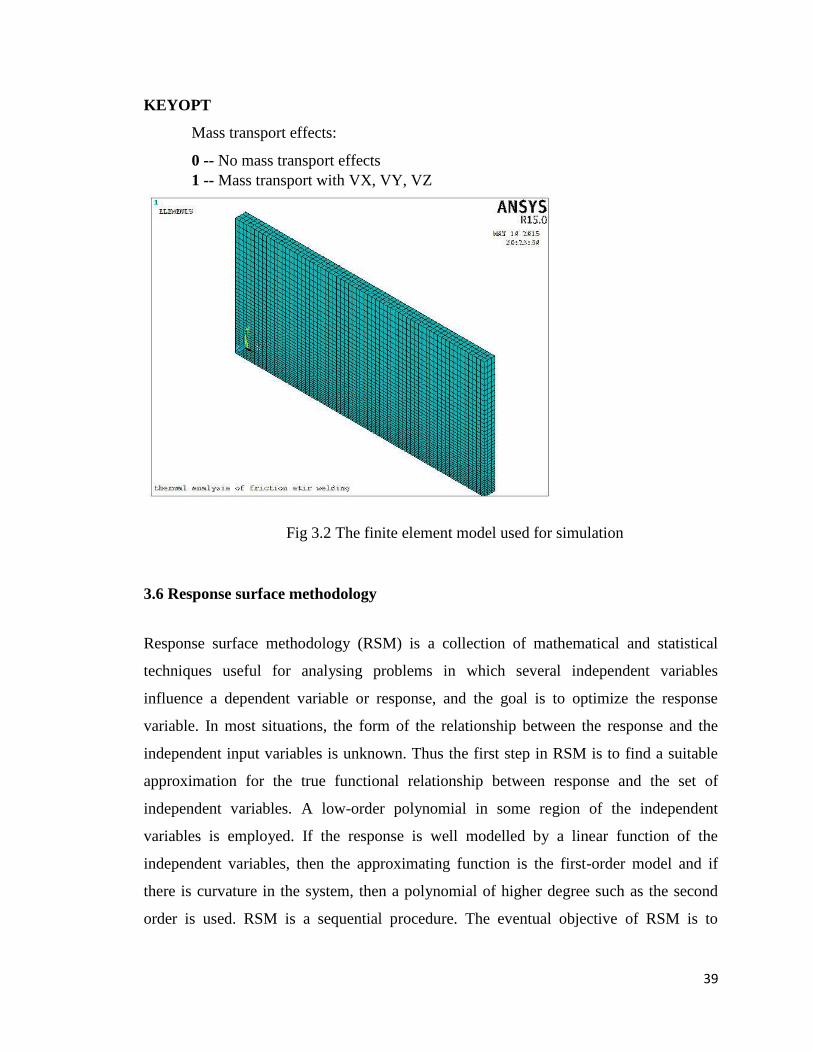
Fig 3.2 The finite element model used for simulation
3.6 Response surface methodology
Response surface methodology (RSM) is a collection of mathematical and statistical
techniques useful for analysing problems in which several independent variables
influence a dependent variable or response, and the goal is to optimize the response
variable. In most situations, the form of the relationship between the response and the
independent input variables is unknown. Thus the first step in RSM is to find a suitable
approximation for the true functional relationship between response and the set of
independent variables. A low-order polynomial in some region of the independent
variables is employed. If the response is well modelled by a linear function of the
independent variables, then the approximating function is the first-order model and if
there is curvature in the system, then a polynomial of higher degree such as the second
order is used. RSM is a sequential procedure. The eventual objective of RSM is to
40
determine the optimum operating conditions for the system, or to determine a region of
the factor space in which the operating specifications are satisfied.
The data generated from the experimentation is used to develop the mathematical models
by regression analysis that gives linear, quadratic and two way interaction effects of the
input parameters. The tensile strength (TS) of the friction stir welded joints is a function
of tool rotational speed (N), welding speed (S), Shoulder diameter (SD) and pin diameter
(PD) and it can be expressed as
𝑌=𝑓 (𝑁, SD, 𝑃, D) (10)
The developed mathematical models are useful for accurately predicting responses (viz.
tensile strength) for the input parameters (viz. tool rotational speed (N), welding speed
(S), shoulder diameter (SD) and pin diameter (PD) in this work).
The second order polynomial (regression equation) used to represent the response surface
for K factors is given by
k k2
o i i ii i ij i j
i 1 i 1 i j
y b b x b x b x x
(11)
Where “bo” is the constant of the regression equation and provides a mean value of the
response factor,"bi" is the linear term, ”bij” is the interaction term, “bii” is the quadratic
term of the polynomial and “e” is the residual error
The coefficients bo, bi, bij and bii are the least square estimates of the polynomial,
representing the response surface. These coefficients represent the strength of the
respective process parameters and their interactions. These are also called the parameters
of the response function. The experiments were designed and analysed using Minitab. For
four factors, the selected polynomial can be expressed as
2 2 2 2
o 1 2 3 4 11 1 22 2 33 3 44 4 12
13 14 23 24 34
TS(MPa) b b (N) b (S) b (SD) b (PD) b x b x b x b x b (N)(S)
b (N)(SD) b (N)(PD) b (S)(SD) b (S)(PD) b (SD)(PD)
(12)
41
Chapter 4: Results and Discussion
4.1 Introduction
Friction Stir Welding of AA1100 was simulated using finite element method. A three
dimension finite element model was built using the finite element package ANSYS. The
element used was solid 70, a three dimensional eight noded brick element. The element
had temperature as the degree of freedom. In this work the material flow has been
neglected as a whole and only the heat transfer aspect has been considered. The tool is
represented as a moving heat flux and the clamps are not considered as the heat loss to
the clamp is negligible due to their small area of contact and location. To reduce the
computational requirements, regions around the weld line are meshed with smaller
element, while the element size farther from the weld line is larger. Convection
coefficient for all the surfaces exposed to atmosphere is 25 W/m2 K. The heat loss to the
backing plate, which is essentially contact conduction, is accounted by using an
equivalent convection coefficient at the bottom of the plates. Temperature dependent
material properties are used for the plates as these give reasonable prediction for transient
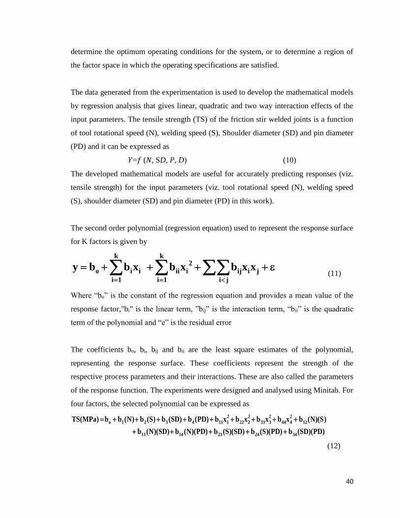
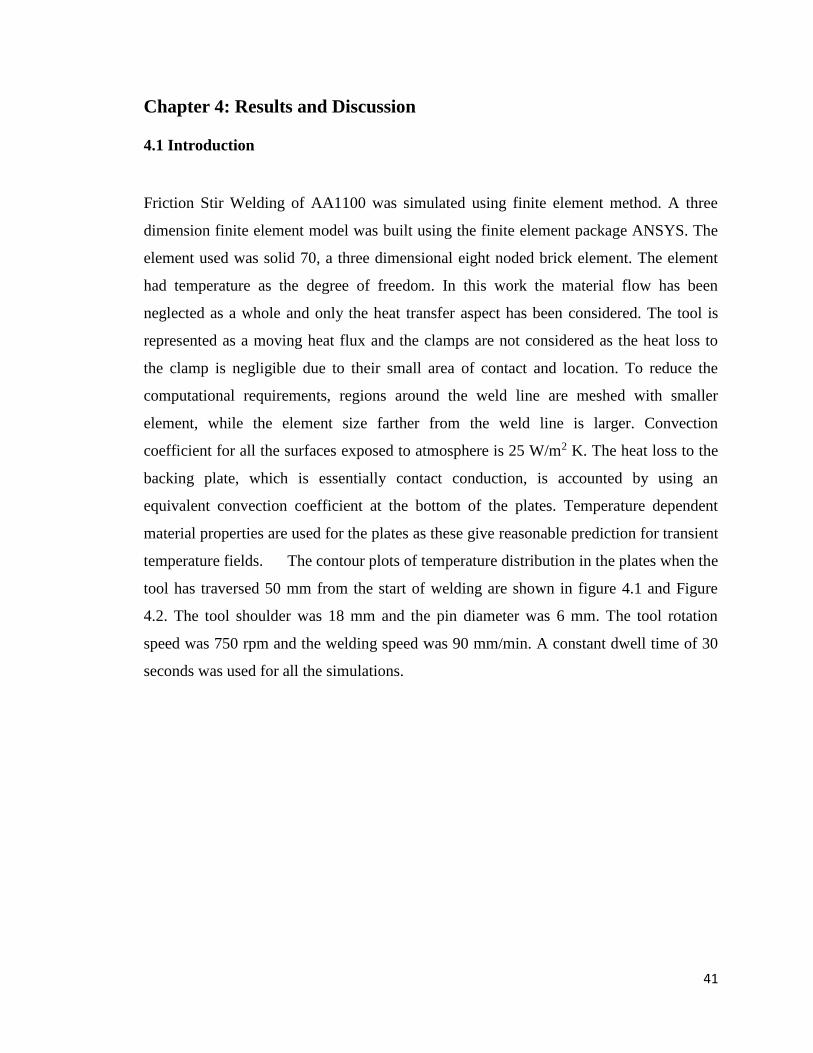
temperature fields. The contour plots of temperature distribution in the plates when the
tool has traversed 50 mm from the start of welding are shown in figure 4.1 and Figure
4.2. The tool shoulder was 18 mm and the pin diameter was 6 mm. The tool rotation
speed was 750 rpm and the welding speed was 90 mm/min. A constant dwell time of 30
seconds was used for all the simulations.
42
Figure 4.1 Temperature contour for Trial 5
Figure 4.2 Temperature contour (cross section) for Trial 5
To study the effect of process parameters on the temperature distribution, the simulation
trials have been tried for different process parameters as given below. The corresponding
maximum temperatures are listed in table 4.2.
43
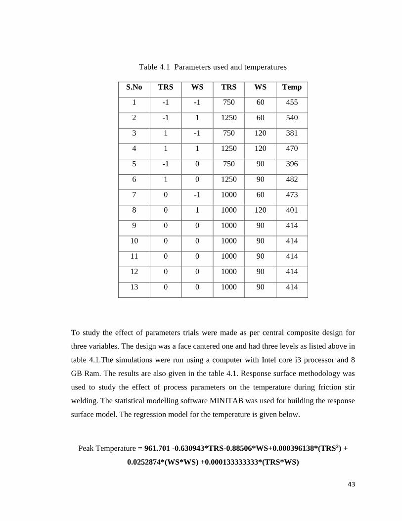
Table 4.1 Parameters used and temperatures
S.No TRS WS TRS WS Temp
1 -1 -1 750 60 455
2 -1 1 1250 60 540
3 1 -1 750 120 381
4 1 1 1250 120 470
5 -1 0 750 90 396
6 1 0 1250 90 482
7 0 -1 1000 60 473
8 0 1 1000 120 401
9 0 0 1000 90 414
10 0 0 1000 90 414
11 0 0 1000 90 414
12 0 0 1000 90 414
13 0 0 1000 90 414
To study the effect of parameters trials were made as per central composite design for
three variables. The design was a face cantered one and had three levels as listed above in
table 4.1.The simulations were run using a computer with Intel core i3 processor and 8
GB Ram. The results are also given in the table 4.1. Response surface methodology was
used to study the effect of process parameters on the temperature during friction stir
welding. The statistical modelling software MINITAB was used for building the response
surface model. The regression model for the temperature is given below.
Peak Temperature = 961.701 -0.630943*TRS-0.88506*WS+0.000396138*(TRS2) +
0.0252874*(WS*WS) +0.000133333333*(TRS*WS)
44
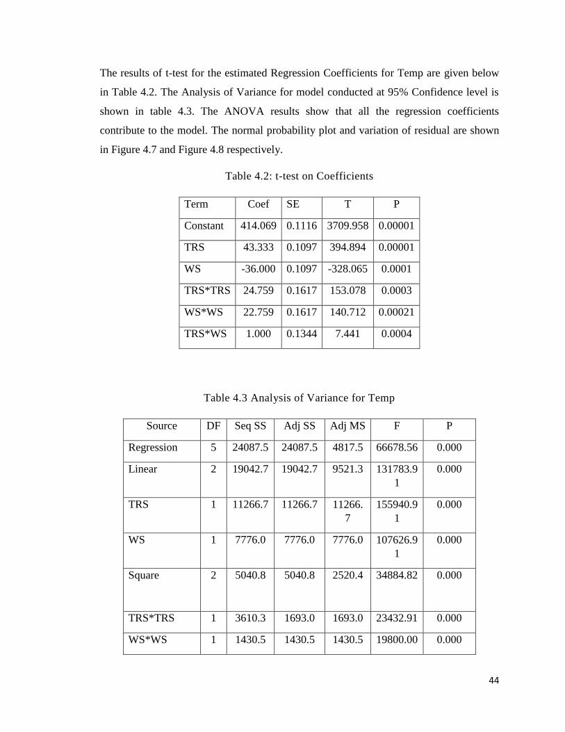
The results of t-test for the estimated Regression Coefficients for Temp are given below
in Table 4.2. The Analysis of Variance for model conducted at 95% Confidence level is
shown in table 4.3. The ANOVA results show that all the regression coefficients
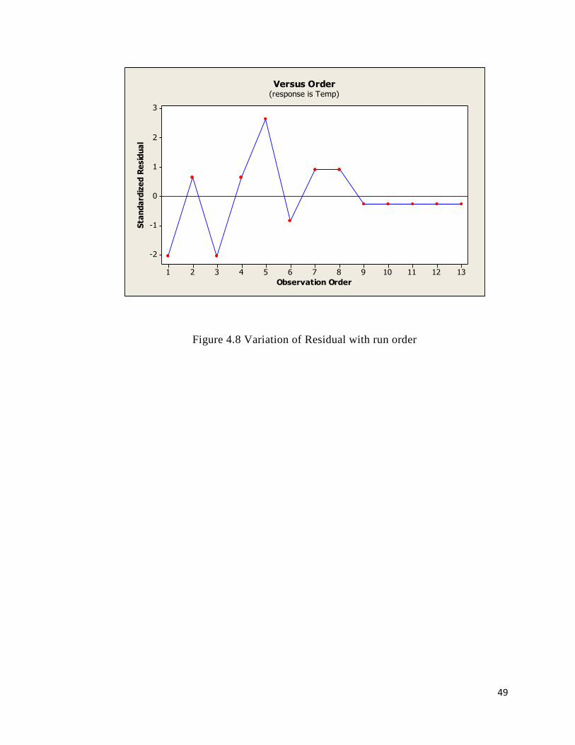
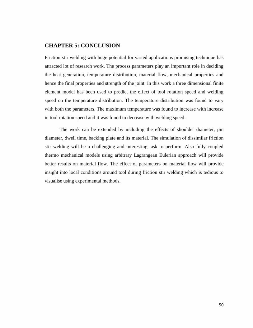
contribute to the model. The normal probability plot and variation of residual are shown
in Figure 4.7 and Figure 4.8 respectively.
Table 4.2: t-test on Coefficients
Term Coef SE T P
Constant 414.069 0.1116 3709.958 0.00001
TRS 43.333 0.1097 394.894 0.00001
WS -36.000 0.1097 -328.065 0.0001
TRS*TRS 24.759 0.1617 153.078 0.0003
WS*WS 22.759 0.1617 140.712 0.00021
TRS*WS 1.000 0.1344 7.441 0.0004
Table 4.3 Analysis of Variance for Temp
Source DF Seq SS Adj SS Adj MS F P
Regression 5 24087.5 24087.5 4817.5 66678.56 0.000
Linear 2 19042.7 19042.7 9521.3 131783.9
1
0.000
TRS 1 11266.7 11266.7 11266.
7
155940.9
1
0.000
WS 1 7776.0 7776.0 7776.0 107626.9
1
0.000
Square 2 5040.8 5040.8 2520.4 34884.82 0.000
TRS*TRS 1 3610.3 1693.0 1693.0 23432.91 0.000
WS*WS 1 1430.5 1430.5 1430.5 19800.00 0.000
45
Interaction 1 4.0 4.0 4.0 55.36 0.000
TRS*WS 1 4.0 4.0 4.0 55.36 0.000
Residual Error 7 0.5 0.5 0.1
Lack-of-Fit 3 0.5 0.5 0.2
Pure Error 4 0.0 0.0 0.0
Total 12 24088
S = 0.268793 PRESS = 4.56900 R-Sq = 99.23% R-Sq(pred) = 99.19% R-Sq(adj) =
99.56%
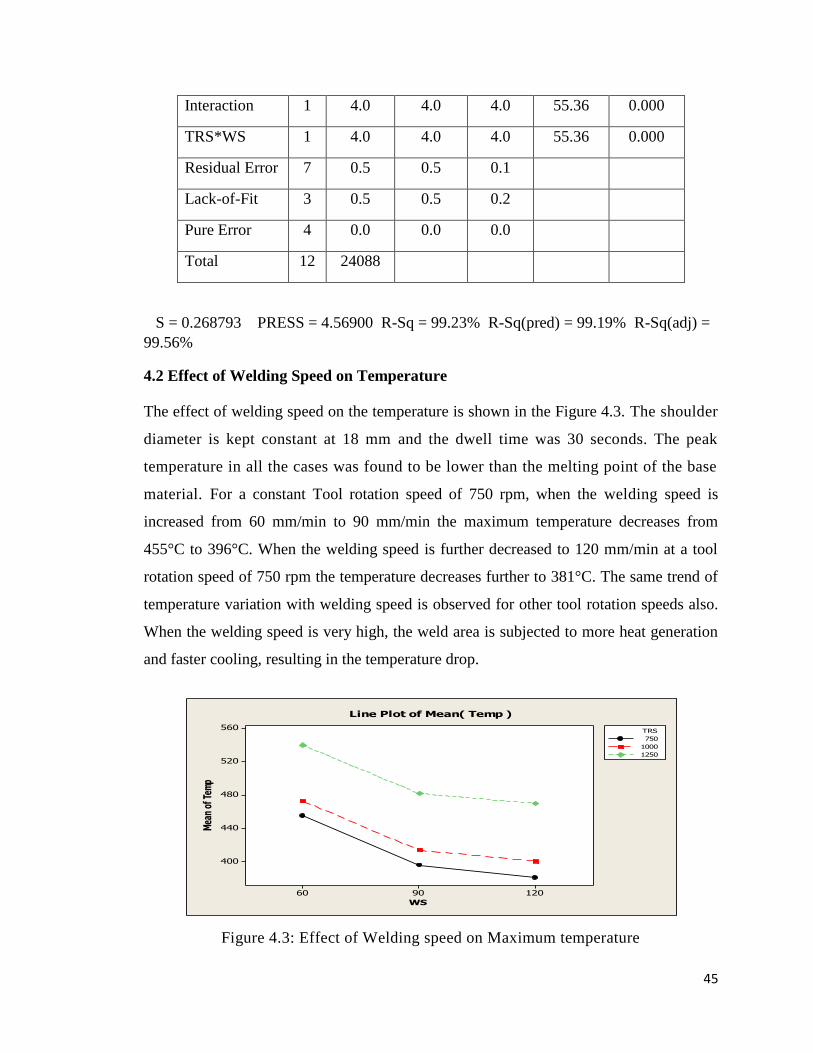
4.2 Effect of Welding Speed on Temperature
The effect of welding speed on the temperature is shown in the Figure 4.3. The shoulder
diameter is kept constant at 18 mm and the dwell time was 30 seconds. The peak
temperature in all the cases was found to be lower than the melting point of the base
material. For a constant Tool rotation speed of 750 rpm, when the welding speed is
increased from 60 mm/min to 90 mm/min the maximum temperature decreases from
455°C to 396°C. When the welding speed is further decreased to 120 mm/min at a tool
rotation speed of 750 rpm the temperature decreases further to 381°C. The same trend of
temperature variation with welding speed is observed for other tool rotation speeds also.
When the welding speed is very high, the weld area is subjected to more heat generation
and faster cooling, resulting in the temperature drop.
1209060
560
520
480
440
400
WS
Mea
n of
Tem
p
750
1000
1250
TRS
Line Plot of Mean( Temp )
Figure 4.3: Effect of Welding speed on Maximum temperature
46
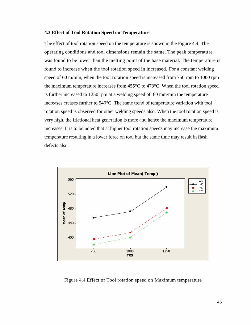
4.3 Effect of Tool Rotation Speed on Temperature
The effect of tool rotation speed on the temperature is shown in the Figure 4.4. The
operating conditions and tool dimensions remain the same. The peak temperature
was found to be lower than the melting point of the base material. The temperature is
found to increase when the tool rotation speed in increased. For a constant welding
speed of 60 m/min, when the tool rotation speed is increased from 750 rpm to 1000 rpm
the maximum temperature increases from 455°C to 473°C. When the tool rotation speed
is further increased to 1250 rpm at a welding speed of 60 mm/min the temperature
increases creases further to 540°C. The same trend of temperature variation with tool
rotation speed is observed for other welding speeds also. When the tool rotation speed is
very high, the frictional heat generation is more and hence the maximum temperature
increases. It is to be noted that at higher tool rotation speeds may increase the maximum
temperature resulting in a lower force on tool but the same time may result in flash
defects also.
12501000750
560
520
480
440
400
TRS
Me
an
of
Te
mp
60
90
120
WS
Line Plot of Mean( Temp )
Figure 4.4 Effect of Tool rotation speed on Maximum temperature
47
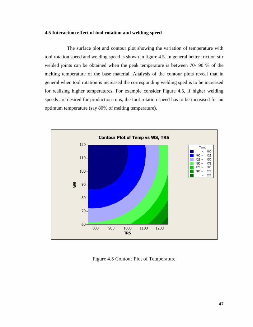
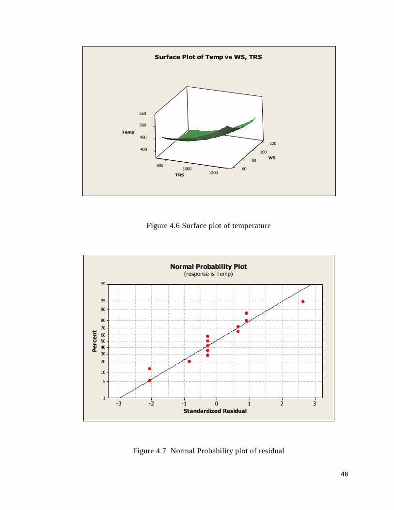
4.5 Interaction effect of tool rotation and welding speed
The surface plot and contour plot showing the variation of temperature with
tool rotation speed and welding speed is shown in figure 4.5. In general better friction stir
welded joints can be obtained when the peak temperature is between 70- 90 % of the
melting temperature of the base material. Analysis of the contour plots reveal that in
general when tool rotation is increased the corresponding welding sped is to be increased
for realising higher temperatures. For example consider Figure 4.5, if higher welding
speeds are desired for production runs, the tool rotation speed has to be increased for an
optimum temperature (say 80% of melting temperature).
TRS
WS
120011001000900800
120
110
100
90
80
70
60
>
–
–
–
–
–
< 400
400 425
425 450
450 475
475 500
500 525
525
Temp
Contour Plot of Temp vs WS, TRS
Figure 4.5 Contour Plot of Temperature
48
120
100400
450
80
500
550
8001000 60
1200
Temp
WS
TRS
Surface Plot of Temp vs WS, TRS
Figure 4.6 Surface plot of temperature
3210-1-2-3
99
95
90
80
70
60
50
40
30
20
10
5
1
Standardized Residual
Pe
rce
nt
Normal Probability Plot(response is Temp)
Figure 4.7 Normal Probability plot of residual
49
13121110987654321
3
2
1
0
-1
-2
Observation Order
Sta
nd
ard
ize
d R
esid
ua
l
Versus Order(response is Temp)
Figure 4.8 Variation of Residual with run order
50
CHAPTER 5: CONCLUSION
Friction stir welding with huge potential for varied applications promising technique has
attracted lot of research work. The process parameters play an important role in deciding
the heat generation, temperature distribution, material flow, mechanical properties and
hence the final properties and strength of the joint. In this work a three dimensional finite
element model has been used to predict the effect of tool rotation speed and welding
speed on the temperature distribution. The temperature distribution was found to vary
with both the parameters. The maximum temperature was found to increase with increase
in tool rotation speed and it was found to decrease with welding speed.
The work can be extended by including the effects of shoulder diameter, pin
diameter, dwell time, backing plate and its material. The simulation of dissimilar friction
stir welding will be a challenging and interesting task to perform. Also fully coupled
thermo mechanical models using arbitrary Lagrangean Eulerian approach will provide
better results on material flow. The effect of parameters on material flow will provide
insight into local conditions around tool during friction stir welding which is tedious to
visualise using experimental methods.
51
REFERENCES
1. W.M. Thomas, E.D. Nicholas, J.C. Needham, M.G. Murch, P. Templesmith, C.J.
Dawes, G.B. Patent Application No.9125978.8 (December 1991).
2. C. Dawes, W. Thomas, TWI Bulletin 6, November/December 1995, p. 124
3. B. London, M. Mahoney, B. Bingel, M. Calabrese, D.Waldron, in: Proceedings of
the Third International Symposium on Friction Stir Welding, Kobe, Japan, 27–28
September, 2001.
4. C.G. Rhodes, M.W. Mahoney, W.H. Bingel, R.A. Spurling, C.C. Bampton,
Scripta Mater. 36 (1997) 69.
5. Chao, Y. J., Qi, X., and Tang, W. 2003.Heat transfer in friction stir welding —
Experimenta land numerical studies, Transaction of the ASME, pp. 125, 138–145
6. Colegrove, P. A., and Shercliff, H. R.2004. Development of Trivex friction stir
welding tool part 1 — two-dimensional flow modeling and experimental
validation. Science and Technology of Welding and Joining 9: 345–351
7. Song, M., and Kovacevic, R. 2002. A new heat transfer model for friction stir-
welding. transaction of NAMRI/SME, SME 30: 565–572.
8. Song, M., and Kovacevic, R. 2003. Thermal modeling of friction stir welding in a
moving coordinate system and its validation. Int. J.of Machine Tools &
Manufacture 43: 605–615.
9. Schmidt, H., Hattel, J., and Wert, J. 2004.An analytical model for the heat
generation in friction stir welding. Modeling and Simulation in Materials Science
and Engineering 12: 143–157.
10. Gould, J. E., and Feng, Z. 1998. Heat flow model for friction stir welding of
aluminum alloys. Journal of Materials Processing & Manufacturing Science
7(2):185–194.
11. Chao, Y. J., and Qi, X. 1998. Thermal and thermo-mechanical modeling of
friction stir welding of aluminum alloy 6061-T6. Journal of Materials Processing
& Manufacturing Science, 7(2): 215–233.
12. Chao, Y. J., Qi, X., and Tang, W., 2003. Heat transfer in friction stir welding —
experimental and numerical studies. ASME Journal of Manufacturing Science and
Engineering 125(1): 138–145.
52
13. Chen, C. M., and Kovacevic, R. 2003. Finite element modeling of friction stir
welding— thermal and thermo-mechanical analysis. Machine Tools &
Manufacture 43: 1319–1326.
14. Song, M., Ouyang, J. H., and Kovacevic, R. 2003. Numerical and experimental
study of heat transfer during friction stir welding of aluminum alloy 6061-T6.
Proceeding of the Institute of Mechanical Engineers, Part B, Journal of
Engineering Manufacture 217(1): 73–85.
15. Nandan, R., Roy, G. G., and Deb- Roy, T. 2006. Numerical simulation of three-
dimensional heat transfer and plastic flow during friction stir welding.
Metallurgical and Materials Transaction A 37(4): 1247–59.