Embed Size (px)
Citation preview
Japan Advanced Institute of Science and Technology
JAIST Repositoryhttps://dspace.jaist.ac.jp/
TitleEffect of thermal degradation on rheological
properties for poly(3-hydroxybutyrate)
Author(s) Yamaguchi, M; Arakawa, K.
Citation European Polymer Journal, 42(7): 1479-1486
Issue Date 2006-07
Type Journal Article
Text version author
URL http://hdl.handle.net/10119/3381
Rights
Elsevier Ltd., Masayuki Yamaguchi and Keiichi
Arakawa, European Polymer Journal, 42(7), 2006,
1479-1486.
http://www.sciencedirect.com/science/journal/0014
3057
Description

Effect of Thermal Degradation on Rheological
Properties for Poly(3-hydroxybutyrate)
Masayuki Yamaguchi and Keiichi Arakawa
School of Materials Science,
Japan Advanced Institute of Science and Technology
1-1 Asahidai, Nomi, Ishikawa 923-1292 JAPAN
Corresponding to Masayuki Yamaguchi School of Materials Science, Japan Advanced Institute of Science and Technology 1-1 Asahidai, Nomi, Ishikawa 923-1292 Japan Phone +81-761-51-1621, Fax +81-761-51-1625 E-mail [email protected]

Yamaguchi 2
ABSTRACT: Thermal degradation at processing temperature and the effect on the
rheological properties for poly(3-hydroxybutyrate) have been studied by means of
oscillatory shear modulus and capillary extrusion properties, with the aid of molecular
weight measurements. Thermal history at processing temperature depresses the viscosity
because of random chain scission. As a result, gross melt fracture hardly takes place with
increasing the residence time in a capillary rheometer. Moreover, it was also found that
the molecular weight distribution is independent of the residence time, whereas the
inverse of the average molecular weight is proportional to the residence time. Prediction
of average molecular weight with a constant molecular weight distribution makes it
possible to calculate the flow curve following generalized Newtonian fluid equation
proposed by Carreau as a function of temperature as well as the residence time.
Key words: poly(3-hydroxybutyrate); rheological properties;
thermal degradation

Yamaguchi 3
INTRODUCTION
Poly(3-hydroxybutyrate) (PHB) and its copolymer have been known as one of the
most famous biopolyesters since the success of isolation and identification in 1926.1
Although the first trial to commercialization, which started in the late 1980s,2 did not
result in the major replacement from conventional plastics because of the poor
cost-performance and the lack of thermal stability, PHB and its copolymer have received
increasing attention these days owing to the rapid growth of the interest in environment.
The thermal degradation of PHB during processing, which is obvious beyond 170 ºC,
occurs even at lower temperature than the melting point of PHB homopolymer, 177 ºC.
Hence, considerable effort has been carried out to develop copolymers with
3-hydroxyvalerate, 4-hydroxybutyrate, or 3-hydroxyhexanoate in order to lower the
melting point, and thus, the processing temperature,2-4 although the copolymerization
loses the rigidity.
Pioneering work on thermal degradation of PHB has been carried out by Grassie
et al.5-7 at various temperatures. They clarified the main reaction occurred at processing
temperature, i.e., between 170 and 200 ºC, is a random chain scission,6 whereas the low
molecular weight compounds are mainly generated by the thermal degradation beyond
300 ºC.5 The random chain scission occurs at ester group, leading to the formation of
carboxyl groups and vinyl crotonate ester groups, through six-membered ring ester
decomposition process,6,7 which was proved by Kunioka and Doi by NMR
measurements.8 Because of the simple first-order reaction, the inverse of number-average
degree of polymerization for the sample is proportional to the residence time t at
processing temperature.6,8 Moreover, Kunioka and Doi also demonstrated that apparent
activation energy of thermal degradation is about 212 kJ/mol, which is independent of the
copolymerization with 3-hydroxyvalerate or 4-hydroxybutyrate.8 Later, Daly et al, also
evaluated the activation energy from the viscous depression, i.e., rheological
characterization, and obtained a similar level of activation energy, 190 kJ/mol.9 Moreover,
Melik and Schechtman found that the degradation rate during processing is basically
independent of the applied shear rate, although temperature rise due to viscous energy
dissipation has an influence on the decomposition.10 Except for the study by Daly et al.
and Melik and Schechtman, however, the rheological properties of PHB homopolymer

Yamaguchi 4
were not investigated in detail because of the complexity attributed to the thermal
instability. The uncertainty of the rheological properties during processing is a serious
problem to operate a processing machine appropriately, and thus, results in poor
processability.
In this study, the linear viscoelastic properties as well as the capillary extrusion
properties were evaluated at processing temperature considering the change of molecular
weight. Further, it is shown that the flow curves during processing are predictable as a
function of the residence time and the resin temperature. The results will have a great
impact on the material design for PHB homopolymer, because it makes easier to control
the processability and the mechanical properties of final products.
EXPERIMENTAL
Materials
The polymer employed in this study was microbial poly(3-hydroxybutyrate)
homopolymer kindly supplied by PHB Industrial S/A in Brazil. The sample was
compressed into a flat sheet by a compression-molding machine (Tester Sangyo,
SA303IS) at 180 ºC for 3 min. After cutting the obtained sheet, various rheological
properties were evaluated.
Measurements
Oscillatory shear moduli, such as shear storage modulus ′ G and loss modulus
, were measured by a cone-and-plate rheometer (UBM, MR500) at various
frequencies as a function of the residence time in the rheometer under a nitrogen
atmosphere at 180 ºC. The cone angle is 2 degree and the diameter of the cone is 25 mm.
After setting the sample immediately between the cone and the plate, which were heated
previously, we collected the oscillatory shear modulus. In this experiment, the Lissajous
pattern can be regarded as closed ellipsoids even at the lowest frequency. We defined t =
0 after 2 min of residence in the rheometer. Further, extrusion properties, such as apparent
shear stress and appearance of extrudates, have been investigated by a capillary
rheometer (Yasuda Seiki Seisakusyo, Capillary Rheometer 140 SAS-2002) also as a
function of the thermal history, i.e., the residence time in the capillary rheometer, at an
′ ′ G

Yamaguchi 5
apparent shear rate of 6.3 s-1. The capillary die employed was 8 mm in length and 2.095
mm in diameter with an entrance angle of π/2. The temperature of the capillary reservoir
cylinder was kept at 180 ºC. We again defined t = 0 at 2 min after putting the sample into
the capillary rheometer. Details in the experimental method about the relation between
residence time and rheological properties were described in the previous papers.11,12
Molecular weight and its distribution were evaluated by a gel permeation
chromatograph, g.p.c., (Tosoh, HLC-8020) with TSK-GEL® GMHXL, as a polystyrene
standard. The thermal history of the sample was applied by the cone-and-plate rheometer
at 180 ºC following the method of the oscillatory measurement. Chloroform was
employed as eluant at 40 ºC at a flow rate of 1.0 ml/min and the concentration of the
sample was 1.0 mg/ml. The g.p.c. characterization was carried out ignoring the oligomer
fraction whose molecular weight is quite different from the main fraction, since the
amount of the oligomer was quite less and independent of the thermal history in this
experiment.
RESULTS
Oscillatory Shear Modulus
Because of chain scission, molecular weight and thus oscillatory modulus
decrease with the residence time in the rheometer at 180 ºC as exemplified in Figure 1.
[Figure 1], [Figure 2]
The depression is more obvious at a lower frequency, demonstrating longer
relaxation time mechanism ascribed to higher molecular weight fraction becomes weak
with increasing the thermal history. Further, the figure indicates that it is impossible to
obtain the frequency dependence of oscillatory shear modulus by a conventional
frequency sweep experiment at 180 ºC. Therefore, collecting the time variation of
oscillatory moduli at various frequencies, we compose the viscoelastic curves as a
function of frequency as shown in Figure 2. The figures demonstrate that applied thermal
history significantly affects the rheological properties even for a short time, which is
comparable with a residence time in a conventional processing machine, such as a

Yamaguchi 6
single-screw extruder and an injection-molding machine. Moreover, three curves of
and at various residence times in Figure 2 are superposed each other by only
horizontal shift as illustrated in Figure 3, suggesting that thermal degradation does not
affect molecular weight distribution. Further, the master curve also indicates that neither
branching nor gelation occurs.
'G
G ′′
[Figure 3]
Capillary Extrusion
Depression of molecular weight, of course, affects the appearance of extrudates as
well as the apparent shear stress at capillary flow. Figure 4 shows the time variation of the
apparent shear stress σ at an apparent shear rate of 6.3 s-1. It is found from the figure that
the apparent shear stress decreases rapidly. The shear stress is a bit larger than the
complex stress measured by oscillatory shear modulus, because neither Bagley nor
Rabinowitsch corrections are carried out.
[Figure 4]
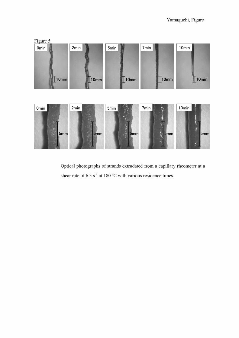
Figure 5 shows optical photographs of the strands extruded by the capillary
rheometer at 180 ºC. As seen in the appearance of the strands shown in the top of the
figure, some extrudates are characterized as wavy shape known as typical distortion
pattern of gross, chaotic, volumetric melt fracture,12-16 which becomes obscure with
increasing the residence time. The results are plausible because the gross melt fracture
often takes place when the melt elasticity, which increases with molecular weight, is
enhanced.12-16 Further, the strand with the residence time of 10 min cannot hold itself
because of less drawdown force. Therefore, the strand falls down by its own weight.
Moreover, it should be noted that the surface roughness of the strands shown in the
bottom of the figure, which is similar to shark-skin failure reported by Zhu et al.
employing poly(3-hydroxybutyrate-co-3-hydroxyvalerate),17 is also improved with the
residence time. The improvement of surface roughness would be attributed to the
reduction of shear stress.13-15,18

Yamaguchi 7
[Figure 5]
The results of the capillary extrusion experiments demonstrate that the residence
time in an extruder or an injection-molding machine has to be seriously taken into
account at the evaluation of flow instability for PHB.
Molecular Weight
As demonstrated by Grassie et al.6 and Kunioka and Doi,8 the inverse of the
number-average degree of polymerization at residence time t is given by the
following relation because the main reaction is a random chain scission, i.e., first-order
reaction, at this temperature;
tNP ,
tkPP d
NtN
=−0,,
11 (1)
where the initial number-average degree of polymerization and the rate constant
of thermal degradation, which is given by Arrhenius relation as follows;
0,NP dk
⎟⎟⎠
⎞⎜⎜⎝
⎛ ∆−=
TkHAkB
d exp (2)
where H∆ the activation energy for the reaction evaluated previously8,10 and the
Boltzmann constant.
Bk
The g.p.c. measurements in this study also confirm that the molecular weight of
PHB follows equation (1) as shown in Figure 6, with a small deviation of the slope from
the previous researches.6,8 Moreover, it was also found that g.p.c. curves do not change its
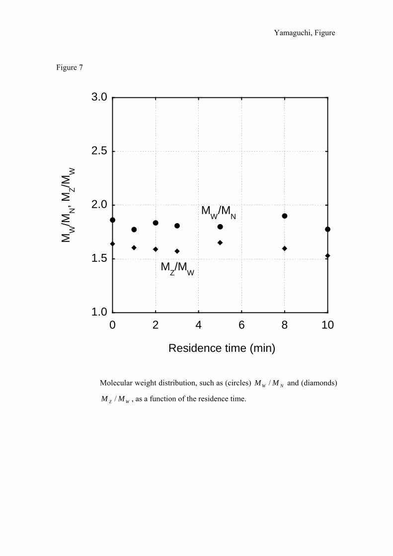
shape with the residence time. Figure 7 shows the molecular weight distributions, such as
and , as a function of the residence time. The g.p.c. results support
the rheological properties in Figure 3.
NW MM / WZ MM /
[Figure 6] [Figure 7]
DISCUSSION

Yamaguchi 8
Figure 7 demonstrates that molecular weight distribution is almost independent of
the residence time whereas the average molecular weight decreases rapidly. Equation (1)
gives the number-average molecular weight as the following simple relation,
0,,
11
N
d
tN Mmtk
M+= (3)
where is the molecular weight of the monomer unit. m
Consequently, is written by; tNM ,
bat
M tN +=
1, (4)
where and . mka d /= 0,/1 NMb =
Further, considering is constant, is expressed by the following relation; NW MM / tWM ,
batcM tW +
=, (5)
where . NW MMc /=
The generalized Newtonian fluid (GNF) representation of the wall shear stress
( )γσ & is given by the product of shear rate γ& and γ& –dependent shear viscosity ( )γη & as,
( ) ( )γγηγσ &&& = (6)
According to the Carreau GNF equation,19,20 shear viscosity of GNF is expressed by
( ) ( )[ ] 21
20 1
−
+=n
wγτηγη && (7)
where 0η the zero-shear viscosity, (0 < n < 1) the dimensionless parameter dependent
on molecular weight distribution, and
n
wτ the weight-average relaxation time defined by
equation (8).
( )
( )0
0
2
ln
lnew J
dH
dHη
τττ
ττττ =≡
∫∫ (8)
where ( )τH the relaxation spectrum and the steady-state compliance. 0eJ
When , equation (7) becomes a simple power law relation as, 1−>> wτγ&
(9) ( ) 1−= nKγγη &&

Yamaguchi 9
where K is so-called consistency.20
Because molecular weight distribution, and thus, n in equation (7), is assumed to
be a constant value, the flow curve of 0/ηη versus γτ &w is independent of the residence
time, whereas both 0η and wτ decrease rapidly. Accordingly, shear viscosity at the
residence time t, ),( tγη & , can be written as;
( ) { }[ ] 21
20 )(1)(,
−
+=n
w ttt γτηγη && (10)
[Table I], [Figure 8]
Table I shows the weight-average molecular weights and zero-shear
viscosities
WM
0η at various residence times, t = 0, 5, and 10 min. It is found that 0η is
proportional to , which is close to the well-known relation,6.3WM 21 i.e., .
Therefore,
4.30 WM∝η
0η at t = 0 is estimated to be 7000 [Pa s]. A fitting curve following equation
(10) with 7000)0(0 =η [Pa s] is shown in Figure 8 with the experimental values of
complex shear viscosity. The fitting curve, denoted by a solid line, gives 5.0=wτ [s] and
n = 0.62.
Considering the empirical relation, , suggested by Mill,7.34.30 )/( −∝ WZe MMJ 21
wτ is crudely proportional to . Since as well as keeps a
constant irrespective of the residence time as demonstrated in Figure 7, is given by;
6.3ZM WZ MM / NW MM /
tZM ,
bat
dM tZ +=, (11)
where is cd / WZ MM / .
Therefore, )(0 tη and )(twτ at a residence time t are given by the initial values at t
= 0, i.e., )0(0η and )0(wτ , as follows;
4.3
00 )0()( ⎟⎠⎞
⎜⎝⎛
+=
batbt ηη (12)
4.3
)0()( ⎟⎠⎞
⎜⎝⎛
+=
batbt ww ττ (13)

Yamaguchi 10
Consequently, the flow curves of the PHB, which are the function of the residence
time, are predictable from equations (10), (12), and (13), as long as )0(0η and )0(wτ are
given.
The predicted values by the equations are also plotted in Figure 8 denoted as
dotted lines with the experimental data of complex shear viscosities represented as
circles. The figure demonstrates that the change of flow curve during processing, i.e.,
applied thermal history, is calculated quantitatively. Further, apparent activation energy
of chain scission reaction reported by Kunioka and Doi and Daly et al. would make it
possible to estimate the flow curve at various processing temperatures. Moreover, the
expression in equation (10) will be widely available for PHB and its copolymers because
microbial polyhydroxyalkanoates, including PHB homopolymer, has a similar molecular
weight distribution,3 i.e., a similar n.
CONCLUSION
Rheological properties for PHB homopolymer at processing temperature have
been studied considering the chain scission reaction during processing. It was found that
the oscillatory shear modulus and the steady-state shear stress decrease with the residence
time in a rheometer in accord with the reduction of molecular weight. Further, the
depression of shear stress and melt elasticity diminishes the onset of gross, chaotic melt
fracture with surface roughness of the extrudates at capillary extrusion. Furthermore, the
inverse of molecular weight is proportional to the residence time in a rheometer with a
constant molecular weight distribution. Finally, the change in the flow curve due to
thermal degradation at processing temperature is successfully predicted by Carreau’s
generalized Newtonian fluid model, which will give useful information on the actual
processing for PHB and its copolymers.
Acknowledgement
The authors express their gratitude to PHB Industrial S/A in Brazil for their kind supply
of the sample employed in the study.

Yamaguchi 11
REFERENCES
1. Lemoigne M. Bull Soc Chem Biol 1926;8:770.
2. Asrar J, Gruys KJ, Biodegradable Polymer Biopol, In: Doi Y, Steinbüchel A,
editors. Biopolymers Vol. 3b. Wiley-VCH; 2002. chapter 3.
3. Abe H, Doi Y, Molecular and Material Design of Biodegradable
Poly(hydroxyalkanoate)s, In: Doi Y, Steinbüchel A, editors. Biopolymers Vol. 3c.
Wiley-VCH; 2002. chapter 5.
4. Satkowski MM, Melik DH, Autran J, Green PR, Noda I, Schechtman LA. Physical
and Processing Properties of Polyhydroxyalkanoate Copolymers, In: Doi Y,
Steinbüchel A, editors. Biopolymers Vol. 3c. Wiley-VCH; 2002. chapter 9.
5. Grassie N, Murray EJ, Holmes PA. Polym Degrad Stab 1984; 6:47.
6. Grassie N, Murray EJ, Holmes PA. Polym Degrad Stab 1984;6:95.
7. Grassie N, Murray EJ, Holmes PA. Polym Degrad Stab 1984;6:127.
8. Kunioka M, Doi Y. Macromol 1990;23:1933.
9. Daly PA, Bruce DA, Melik DH, Harrison GM. J Appl Polym Sci 2005;98:66.
10. Melik DH, Schechtman LA. Polym Eng Sci 1995;35:1795.
11. Yamaguchi M, Gogos CG. Adv Polym Technol 2001;20:261.
12. Yamaguchi M. J Appl Polym Sci 2001;82:1277.
13. Tordella JP. In: Erich FR, editor. Rheology. New York: Academic Press; 1969. p.57.
14. White JL. Appl Polym Symp 1973;20:155.
15. Cogswell FN. Polymer Melt Rheology. New York: Wiley; 1981.
16. Yamaguchi M, Todd DB, Gogos CG. Adv Polym Technol 2003;22:179.
17. Zhu Z, Dakwa P, Tapadia P, Whitehouse RS, Wang S. Macromol 2003;36:4891.
18. Yamaguchi M, Miyata H, Tan V, Gogos CG. Polym 2002;43:5249.
19. Carreau PJ. Ph.D. thesis, Univ. Wisconsin, 1968.
20. Tadmor Z, Gogos CG. Principles of Polymer Processing, New York: Wiley; 1979.
chapter 6.
21. Ferry JD. Viscoelastic Properties of Polymers. New York: Wiley; 1980.

Yamaguchi 12
Figure Captions
Figure 1 Residence time dependence of shear storage modulus (○) and loss
modulus G (●) at 180 °C at (a) 0.1 Hz, (b) 1 Hz, and (c) 10 Hz for PHB.
'G
′′
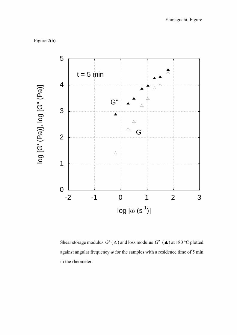
Figure 2 Shear storage modulus 'G (○) and loss modulus G ′′ (●) at 180 °C plotted
against angular frequency ω for the samples with various residence times in
the rheometer; (a) 0 min, (b) 5 min, and (c) 10 min.
Figure 3 Master curves of shear storage modulus (open symbols) and loss
modulus (closed symbols) at 180 °C for the samples with various
residence times in the rheometer; (circles) t = 0 min, (triangles) t = 5 min,
and (diamonds) t = 10 min. a
'G
G ′′
D is the shift factor, and the residence time for
the reference sample is 0 min, i.e., aD = 1.
Figure 4 Apparent shear stress σ at a shear rate of 6.3 s-1 plotted against the
residence time at 180 °C.
Figure 5 Optical photographs of strands extrudated from a capillary rheometer at a
shear rate of 6.3 s-1 at 180 ºC with various residence times.
Figure 6 Inverse of number-average molecular weight, , against the residence
time in the rheometer at 180 ºC.
NM/1
Figure 7 Molecular weight distribution, such as (circles) and (diamonds)
, as a function of the residence time.
NW MM /
WZ MM / Figure 8 Experimental data of absolute value of complex shear viscosity
for the sample with various residence times at 180 ºC; circles t = 0 min,
triangles t = 5 min, and diamonds t = 10 min. In the figure, a fitting curve by
equation (10) with
) ;(* tωη
7000)0(0 =η [Pa s] is represented by a solid line. The

Yamaguchi 13
dotted lines are the predicted ones at t = 5 and 10 min from equation (10)
considering the parameters given by the fitting curve.
Table 1 Weight-average molecular weight and zero-shear viscosity at various residence
times
Residence time
in a rheometer (min)
Weight-average molecular
weight, MW
Zero-shear viscosity, η0
(Pa s)
0 434,000 -
5 302,000 1140
10 228,000 313

Yamaguchi, Figure
Figure 1(a)
0
1
2
3
4
5
6
0 2 4 6 8 10
log
[G' (
Pa)
], lo
g [G
" (P
a)]
Residence time (min)
0.1 Hz
G"
G'
12
Residence time dependence of shear storage modulus (○) and loss
modulus G (●) at 180 °C at 0.1 Hz for PHB.
'G
′′

Yamaguchi, Figure
Figure 1(b)
0
1
2
3
4
5
6
0 2 4 6 8 10
log
[G' (
Pa)
], lo
g [G
" (P
a)]
1 Hz
G"
G'
Residence time (min)
12
Residence time dependence of shear storage modulus (○) and loss
modulus G (●) at 180 °C at 1 Hz for PHB.
'G
′′

Yamaguchi, Figure
Figure 1(c)
0
1
2
3
4
5
6
0 2 4 6 8 10
log
[G' (
Pa)
], lo
g [G
" (P
a)]
10 Hz
G"
G'
Residence time (min)
12
Residence time dependence of shear storage modulus (○) and loss
modulus G (●) at 180 °C at 10 Hz for PHB.
'G
′′

Yamaguchi, Figure
Figure 2(a)
0
1
2
3
4
5
-2 -1 0 1 2 3
log
[G' (
Pa)
], lo
g [G
" (P
a)]
log [ω (s-1)]
G'
G"t = 0 min
Shear storage modulus 'G (○) and loss modulus G ′′ (●) at 180 °C plotted
against angular frequency ω for the samples with a residence time of 0 min
in the rheometer.
Yamaguchi, Figure
Figure 2(b)
0
1
2
3
4
5
-2 -1 0 1 2 3
log
[G' (
Pa)
], lo
g [G
" (P
a)]
log [ω (s-1)]
G'
G"
t = 5 min
Shear storage modulus 'G ( ∆ ) and loss modulus G ′′ (▲) at 180 °C plotted
against angular frequency ω for the samples with a residence time of 5 min
in the rheometer.

Yamaguchi, Figure
Figure 2(c)
0
1
2
3
4
5
-2 -1 0 1 2 3
log
[G' (
Pa)
], lo
g [G
" (P
a)]
log [ω (s-1)]
G'
G"
t = 10 min
Shear storage modulus ' (◇) and loss modulus G G ′′ (◆) at 180 °C plotted
against angular frequency ω for the samples with a residence time of 10 min
in the rheometer.

Yamaguchi, Figure
Figure 3
0
1
2
3
4
5
-2 -1 0 1 2 3
log
[G' (
Pa)],
log
[G" (
Pa)]
log [ωaD (s-1)]
t = 0 min180 C
G"
G'
Master curves of shear storage modulus and loss modulus at 180 °C
for the samples with various residence times, t = 0, 5, 10 min, in the
rheometer; The symbols are the same as in Figure 2. a
'G G ′′
D is the shift factor,
and the residence time for the reference sample is 0 min, i.e., aD = 1.

Yamaguchi, Figure
Figure 4
0
0.1
0.2
0.3
0 2 4 6 8
log
[σ(t)
(MP
a)]
Residence time (min)
180 C
10
Apparent shear stress σ at a shear rate of 6.3 s-1 plotted against the
residence time at 180 °C.
Yamaguchi, Figure
Figure 5
10mm10mm10mm10mm10mm
0min 2min 5min 7min 10min
5mm 5mm 5mm 5mm 5mm
0min 2min 5min 7min 10min
10mm10mm10mm10mm10mm10mm10mm10mm10mm
0min 2min 5min 7min 10min
5mm5mm 5mm5mm 5mm5mm 5mm5mm 5mm5mm
0min 2min 5min 7min 10min
Optical photographs of strands extrudated from a capillary rheometer at a
shear rate of 6.3 s-1 at 180 ºC with various residence times.

Yamaguchi, Figure
Figure 6
0 2 4 6 8
Mn-1
x 1
06 (mol
/g)
Residence time (min)
10
8
6
4
2
0
180 C
10
Inverse of number-average molecular weight, , against the residence
time in the rheometer at 180 ºC.
NM/1
Yamaguchi, Figure
Figure 7
1.0
1.5
2.0
2.5
3.0
0 2 4 6 8
MW
/MN, M
Z/MW
Residence time (min)
MW
/MN
MZ/MW
10
Molecular weight distribution, such as (circles) and (diamonds)
, as a function of the residence time.
NW MM /
WZ MM /

Yamaguchi, Figure
Figure 8
log
[η*
(ω; t
) (P
a s)
]
log [ω (s-1)]
-1 0 1 2
2
3
1
4
180 C
t = 10 min
t = 5 min
t = 0 min
Experimental data of absolute value of complex shear viscosity
for the sample with various residence times at 180 ºC; circles t = 0 min,
triangles t = 5 min, and diamonds t = 10 min. In the figure, a fitting curve by
equation (10) with
) ;(* tωη
7000)0(0 =η [Pa s] is represented by a solid line. The
dotted lines are the predicted ones at t = 5 and 10 min from equation (10)
considering the parameters given by the fitting curve.