Bmail

EFFECT OF WIND FARMS AT THE

NORTH SEA ON METEOROLOGICAL

CONDITIONS IN THE NETHERLANDS

An analyses of the most gross weather types

Duin, Mathijs mathijs.duin@wur.nl

MSc Thesis in Meteorology and Air Quality

Mathijs Duin Supervised by Gert-Jan Steeneveld

April 2nd 2019

1

Abstract In recent years the production of wind energy in the Netherlands and the European Union has substantially

increased (Global Wind Energy Council, 2017). In 2017, the wind energy production in Europe increased

with 16.8 GW to 177.5 GW. In the Netherlands, the amount of wind energy increased with 81 MW in 2017.

This increase in wind energy generation raises concerns about the effect of wind farms on climate

downwind. This study deals with the effect of wind farms on changes in weather patterns in the

Netherlands. To make a climatological overview, we selected seven events in summer and seven events

in winter. Each event represents a certain gross weather type. This study is performed in WRF, using a

very fine resolution of 3 x 3 km. The wind farms modelled in WRF are based on a future scenario in which

the wind turbines are equipped by 8 MW turbines. We conclude that the average 10-m wind speed around

the wind farms decreases up to 1 m/s, which logically has influence on the expected available wind energy.

Side effects on humidity, radiation and temperature are found as well. Humidity decreases in general

directly vertically above the wind farms by 0.04 g/kg outside of wind farms areas. In general, less

shortwave-in radiation occurs at the wind farms. However, more shortwave-in radiation will be received

east of the wind farms, for example in the western part of the Netherlands. The changes in temperature

are more variable. However, on average, the temperature in the western part of the Netherlands decreases

by 0.1 K in winter and 0.2 K in some individual case runs.

2

Table of Contents Abstract ................................................................................................................................... 1

1. Introduction ................................................................................................................... 3

2. Research questions .......................................................................................................... 4

3. Methodology ................................................................................................................... 4

3.1. Case selection ............................................................................................................. 4

3.2. Model setup ................................................................................................................ 5

3.3. Wind farm parametrisation ............................................................................................ 5

3.4. Model validation and statistical analyses .......................................................................... 6

3.5. Model parameters ........................................................................................................ 6

4. Results .......................................................................................................................... 8

4.1. Validation ................................................................................................................... 8

4.2. Change in climatology ................................................................................................ 11

4.2.1. Wind speed ........................................................................................................... 11

4.2.2. Temperature .......................................................................................................... 13

4.2.3. Humidity ............................................................................................................... 14

4.2.4. Precipitation .......................................................................................................... 14

4.2.5. Solar radiation and clouds ....................................................................................... 14

4.3. Individual cases ......................................................................................................... 16

4.3.1. Wind Speed ........................................................................................................... 16

4.3.2. Humidity ............................................................................................................... 17

4.3.3. Solar radiation and clouds ....................................................................................... 17

4.3.4. Temperature .......................................................................................................... 17

4.3.5. Precipitation .......................................................................................................... 19

5. Discussion .................................................................................................................... 25

6. Conclusion.................................................................................................................... 27

References ........................................................................................................................ 28

Acknowledgements ............................................................................................................. 30

Appendix ........................................................................................................................... 30

3

1. Introduction In the recent years the production of wind energy in the Netherlands and the European Union has

increased substantially. In the Netherlands, the amount of wind energy increased with 81 MW in 2017. In

the UK, the increase in amount of wind energy is much larger, to be exactly: 4270 MW (Global Wind

Energy Council, 2017). Also, in the coming years, the amount of energy gained by wind turbines will

increase (Ministerie van Economische Zaken en Klimaat, 2018). In the so called “energieakkoord”

(energy agreement) of the Netherlands states that 16% of the energy production should be renewable in

2023. The ambitions for 2050 are even higher; then 90 – 95 % of the energy production should originate

from renewable resources (Ministerie van Economische Zaken, & Ministerie van Volkshuisvesting en

Milieubeheer, 2018). In this plan, renewable energy resources should be built. Wind energy is one of

these renewable resources on the North Sea. The countries around the North Sea are building more and

more wind farms. Though, some countries build more than other countries (Tom Remy, 2018). Also the

Netherlands aim to increase the amount of wind energy. For this reason some new wind farms are

planned, especially between 2024 and 2030. In these years the total wind power production of the

Netherlands should increase from respectively 4.5 to 11.5 GW (Ministerie van Economische Zaken en

Klimaat, 2018). In 4cOffshore, an image of all actual and projected wind arms is presented.

Due to this increase in wind farm application, we start to concern what the effect is on weather patterns.

Increasing surface friction logically reduces the wind speed. In earlier studies, the effect of wind farms on

different scales has been found (e.g. Lauridsen & Ancell, 2018; Platis et al., 2018; Vautard et al., 2014).

Just an example, according to Platis et al. (2018), the decrease in wind speed is higher in stable

boundary layers than in unstable boundary layers.

Local influences of wind farms have already been quite well studied. After applying wind farms, the 2-m

temperature increases by 0.72 K (Zhou et al., 2012). This also means that the day-night difference in

temperature decreases (Lauridsen & Ancell, 2018). Other studies found comparable surface temperature

changes of 1-2 K (Fitch, Olson, & Lundquist, 2013). For example, Slawsky et al. (2015) found a lower

change in temperature by using remote sensing data, depending on the different surfaces and

conditions, between 0.18 and 0.70 K.

Another local influence of wind turbines is the reduction in day-night temperature difference (Zhou et al.,

2012). This reduction may prevent plants from freezing. For this reason, it is useful to install a wind

turbine next to a field with a frost-intolerant crop or trees (Xia & Zhou, 2017).

These studies made clear that the influence of wind farms on local weather is evident. However, even on

continental scale, wind farms can have an influence on the presence of different weather systems in

winter caused by a more anticyclonic circulation over Europe (Vautard et al., 2014). In such an extreme

case, maybe even the weather predictions should be changed.

In this thesis, I studied the effect of wind farms on the scale of weather patterns in between local and

continental scale. To be exact, I studied the effect of wind farms on the North Sea on weather patterns in

the Netherlands. Since the Netherlands has, most often, a westerly circulation (Werner & Gerstengarbe,

2010), this country is mostly located downwind of these windfarms. In this thesis I will discuss the

situation of the wind farms on the North Sea with all planned wind farms included (Tom Remy, 2018).

On the mesoscale, already some research has been done. Examples of studies on these themes are

Slawsky et al. (2015), who studied on a domain of less than 50 x 50 km in Illinois (USA). Another

example is Pryor et al. (2018), who studied the effect of multiple windfarms on the domain of Iowa

(USA). Similar studies are done over land, but in China (e.g. Sun, Luo, Zhao, & Chang, 2018; Yuan et

al., 2017). These areas have something in common with the North Sea, because these areas are open

areas too. However, the wind farms out of these four studies are located over land, where the large

projected wind farms of the Netherlands are projected over sea.

4

Jiménez et al. (2015) performed already a study about the downwind effect of wind farms over the sea.

They studied the Hornsrev, located in the exclusive economic zone of Denmark, close to its west coast.

They found still an effect 15 km downwind of the windfarm using a model resolution of 333 m.

Unfortunately, the surface area of this wind farm is limited in size. The area of the wind farm is 21 km2

(4cOffshore). As already mentioned in the introduction, the North Sea countries have large ambitions to

build wind farms much larger than the Hornsrev. Possibly, a larger wind farm means a larger effect or an

effect over a larger area.

Summarised, this means that some studies have already been done on the local scale, the continental

scale and over land. According to our knowledge, studies on the effect of wind farms in a marine

environment on a regional scale are currently. In this study, we modelled the effect of a realistic future

pattern of wind farms on wind speed, temperature, humidity, and radiation.

In this thesis first the methodology will be described. Afterwards the results of all gross weather types

will be discussed, before a weighted climatological average will be made.

2. Research questions Based on previous studies and the present knowledge gap, we can define the research question related to

the effect of wind warms on the atmosphere downwind:

- What is the effect of wind farms in the North Sea on weather patterns along the coast of the

Netherlands?

Sub question for this topic are:

o How much is the reduction in wind speed?

o In which areas is this reduction in wind speed?

o How much does the precipitation change?

o What is the change in temperature?

o What is the change in specific humidity?

3. Methodology In this section the methodology of this research will be discussed. At first, the meteorological cases will

be selected. After the case selection the model setup will be discussed. This will be continued with the

wind farm parameterisation in the model setup. Finally the data analyses methods will be discussed.

3.1. Case selection The WRF simulations are performed for the most 7 common large-scale weather types (gross weather

types) (Grabau, 1987) in the Netherlands in winter and in summer. The most common gross weather types

in North-West Europe are a western, northern, calm weather, eastern, north-western, southern, and south-

western circulation (Werner & Gerstengarbe, 2010). These 7 gross weather types together represent 97

% and 96 % of all weather patterns in winter and summer respectively. For each gross weather type, a

typical 8-day event is selected. The case selection strategy is based on the case selection strategy of

Koopmans et al. (2015). They selected the cases from Werner & Gerstengarbe (2010), who identified the

gross weather type of each day in approximately the last century for Germany. However, this research

focusses on the North Sea, which means that it is important to check if the gross weather type is the same

at the North Sea as in Werber & Gerstengarbe (2010). In this study, it is important to analyses a weather

pattern which is constant and stable for a relatively long time. For that reason, all cases have a duration,

excluding spinup time, of 7 days. The 24 hours before the event starts are used as spinup time, like in

Koopmans et al. (2015). The selected cases are described in table 1.

5

Table 1 Gross weather types, occurrence of each gross weather type and the selected events for

this thesis . Case selection partly based on Koopmans et al. (2015)

Gross

weather

type

Description Winter season Weight

in

winter

Summer season Weight

in

summer

W Westerly

circulation

December 1st 1999 –

December 8th 1999

28.8 % June 28th 2004 –

July 5th 2004

25.0 %

SW South-westerly

circulation

December 1st 2000 –

December 8th 2000

6.3 % April 27th 2003 –

May 4th 2003

3.8 %

NW North-westerly

circulation

January 16th 2000 –

January 23rd 2000

7.9 % September 5th 2001 –

September 12th 2001

9.0%

HM Calm weather December 7th 2004 –

December 14th 2004

17.2 % July 23rd 2001 –

July 30th 2001

16.0 %

N Northerly

circulation

February 14th 2005 –

February 21st 2005

13.4 % June 24th 2000 –

July 1st 2000

18.4 %

E Easterly

circulation

February 14th 2003 –

February 21st 2003

15.4 % April 4th 2002 –

April 11th 2002

15.5 %

S Southerly

circulation

October 14th 2000 –

October 21st 2000

8.0 % July 30th 1994 –

August 6th 1994

8.6 %

3.2. Model setup This study is performed using WRF version 3.7.1 (Skamarock et al., 2008). An advantage WRF is its

windfarm parameterisation (Fitch et al., 2012). For the actual weather conditions, operational analyses

data with a 6 hour resolution based on a 0.25 degree spatial resolution of the European Centre of Median-

range Weather Forecast (ECMWF) is used. This because a lot of weather services also use ECMWF boundary

conditions and because WRF is able to implement ECMWF data.

The vertical resolution is such that the lowest 100 meters are covered by 6 vertical grid cells. The model

heights are presented in the appendix. The horizontal resolution should be not more than 5 times the rotor

diameter (Fitch et al., 2012). The rotor size of different wind turbines vary, but nowadays rotors exist with

a diameter of 167 m (WINDPOWER). For modelling a wind farm covered by turbines with rotor diameters

of this size, a minimal horizontal resolution of more than 835 m is required. High resolution modelling

takes of course a lot of time. For this reason the resolution of the inner domain is 3 km x 3 km. This

resolution is still sufficient to resolve convection (Pryor et al., 2018). The outer domain, which should be

large enough to cover entire weather systems, can be much larger. The outer domain contains a resolution

of 15 km x 15 km. The inner domain is nested in this outer domain. The locations of the two nested

domains are presented in figure 1.

Because at least one of the selected cases contains precipitation at a temperature close to 0ºC, a high-

class microphysics scheme developed by Hong & Lim (2006) is used. Because the wind farm

parameterisation of Fitch et al. (2012) uses the MYNN boundary-layer physics scheme, this scheme is used

in this thesis. The feedback from inner to outer domain is switched off. When this feedback was switched

on, an unrealistic difference appeared in the outer domain between the grid cells which are also covered

by the inner domain and the grid cells which are not covered by the inner domain.

3.3. Wind farm parametrisation The wind turbines in WRF are parameterised according to the scheme developed by Fitch et al. (2012). A

difference between this wind turbine parameterisation scheme and previous parameterisation schemes is

that this scheme converts kinetic energy into turbulent kinetic energy and electric energy based on a thrust

coefficient and a power curve (Fitch et al., 2012). This thrust coefficient is based on the study of a modern

commercial wind turbine (Fitch et al., 2012). The thrust coefficient is a non-dimensional coefficient which

quantifies the stow caused by the wind hitting the turbine (Bianchi, Battista, & Mantz, 2007). The

commercial wind turbine on which the power curve and thrust coefficient are based is of the type Vestas

V164 and has a maximum power of 8 MW. The power curve and thrust coefficient of this wind turbine are

described by Desmond, Murphy, Blonk, & Haans (2016) and presented in figure 3. The rotor diameter of

this wind turbine is 164 m (Desmond et al., 2016).

6

For each gross weather type, a run including and a run excluding windfarms is performed. The turbines

are located at present wind parks, future wind parks, planned wind parks and projected wind parks

described in 4COffshore. These locations are obtained at 4cOffshore (4cOffshore). In figure 2 the locations

of these wind parks are presented. Within these wind farms the wind turbines are positioned at a raster of

0.01 degree longitude x 0.02 degree latitude. To avoid boundary problems, only wind farms located more

than 3 grid cells within the boundary of the inner domain are modelled. The wind farm parameterisation is

only switched on in the inner domain and not in the outer domain. When the wind turbine parameterisation

is switched on in both domains, the same wind turbines may be taken into account twice, once in the inner

domain and once in the outer domain.

3.4. Model validation and statistical analyses First, the runs are averaged per simulation. These average results will be described in the “individual

results” section. Second, the results of all gross weather types are merged using a weighted average made

for quantifying the effect of the wind farms. The weight of the contribution of each gross weather type is

the fraction of occurrence of this weather type. The weight is presented in table 1.

The output of the control run is validated with hourly weather station observations obtained by the national

meteorological institute of the Netherlands (KNMI, retrieved at 09/24/2018) and hourly data of North Sea

stations (KNMI, retrieved at 09/24/2018). Locations of the validation points are presented in figure 2.

3.5. Model parameters A list of model parameters, used in the namelist is presented in the appendix.

Figure 1 Map of the two domains

7

Figure 2 Power curve used in this study, based on Desmond et al. (2016)

Figure 3 Map of the North Sea basin with the location of wind parks and locations of KNMI weather observations: A = De Kooy, B = Schiphol, C = De Bilt, D = Leeuwarden, E = Deelen, F =

Groningen, G = Vlissingen, H = Rotterdam, I = Eindhoven, J = K13 K = F3, L = Maastricht, M = Europlatform, N = Twenthe

0

1000

2000

3000

4000

5000

6000

7000

8000

9000

0 5 10 15 20 25 30

Po

we

r (k

W)

wind speed (m/s)

Power curve based on Desmond et al., 2016

8

4. Results First, the model performance of the control runs will be discussed. Second, the change in climate due to

the wind farms will be discussed. This change in climate is based on a weighted average of different runs

in which each of them represent a gross weather type. Finally, the individual contribution of each

simulation will be discussed.

4.1. Validation The validation is performed for all KNMI observation stations highlighted in figure 2. The results of this

validation is presented in figure 4 -7. The averaged values of all gross weather types are weighted averages

where the weight is presented in table 1. The wind measurement equipment of the KNMI, used for this

validation, is required to have a maximal average error of 0.5 m/s (KNMI, 2001). On average, the wind

speed is overestimated by 0.15 m/s, which is smaller than the maximal measurement error of the KNMI

wind measurement equipment (KNMI, 2001). This overestimation is similar in summer and in winter. In

general, land locations show larger under- and overestimations in model wind speed than marine locations.

The average absolute error for wind speed is between 1.1 and 1.7 m/s on all analysed observation stations.

On average, the absolute wind error amounts to 1.33 m/s with a small difference between winter and

summer and between land located observation stations and marine observation stations. Regarding the

wind directions, the simulation with the largest absolute wind errors is the summer simulation with a

dominating southern wind circulation.

The average bias is quite comparable or even better than biases found in literature (Giannakopoulou &

Nhili, 2014; X. M. Hu, Klein, & Xue, 2013). Giannakopoulou & Nhili (2014) found a similar bias when the

MYNN scheme was used. Important to mention is that this study focussed on large parts of Europe, in

which, next to sea and low relief areas, also areas with more relief are included. Hu et al. (2013) found a

larger positive bias of 0.3 m/s. Their bias is larger than the bias found in this study, but their study was

focussing on a land located on a land covered area in Oklahoma (USA) using the YSU scheme. On the

contrary, the absolute error in this study is nearly 50 % larger than in Giannakopouou & Nhili (2014),

because they found an average wind bias of 0.91 m/s. Because the absolute error is approximately constant

with height in Giannakopoulou & Nhili (2014), if using the MYNN scheme, the 10 m error could be estimated

with a similar magnitude. However, Hu et al. (2013) found a root mean squared error of 1.3 m/s using

either the YSU or the MYJ scheme, which is comparable to the average absolute error in this study for land

located stations.

For the 2-m temperature this is different. It is important to notice that the KNMI thermometers have a

measurement uncertainty. For average hourly temperature values, which are used to validate the model

performance, the measurement uncertainty amounts to 0.1 K (Bijma, 2012). On average, the model

temperatures are lower than the observed temperatures. This underestimation occurs at all stations in

summer, and all stations in winter except F3 and K13, which are both located in the North Sea. At these

stations, the model overestimates the temperature in winter. On the contrary, over land, the negative

model bias is strong, with a magnitude of 0.9 K and 1.1 K in winter and summer respectively. These errors

are much larger than the measurement errors of the measurement equipment. Another study found a

negative bias in their model comparison as well (X.-M. Hu, Nielsen-Gammon, & Zhang, 2010). They found

an average negative 2-m temperature bias of 1.25, 0.63 and 0.9 K for the MYJ (Mellor-Yamada-Janic),

YSU (Yonsei University), and ACM2 (asymmetric convective model, version 2) boundary-layer schemes

respectively over south-east Texas. Also Hu et al. (2013) found mean temperature bias of 0.54 K using

the MYJ scheme in a study focussing on Oklahoma (USA). However, in the same study nearly no model

bias was modelled when using the YSU scheme.

The temperature biases and absolute errors are compared to García-Diez, Fernández, Fita, & Yagüe (2013),

who did a study on model temperature biases at various locations in Europe using different boundary layer

schemes. In summer, the majority of their simulations found a negative bias in summer too, which agrees

with this study. On the contrary, they found a positive temperature bias in winter, but with a large standard

9

deviation. The negative winter model temperature bias of 0.66 K fits still in the standard variation of the

majority of the simulations of García-Diez et al. (2013).

The temperature underestimation of our simulations is also visible in the absolute temperature error. All

land located stations, including coastal stations, have an absolute temperature error over 1.3 K in winter

and, except for De Kooy, over 1.8 K in summer which is similar to other studies. These simulations perform

worse over land in summer compared to García-Diez et al. (2013) and comparable to Hu et al. (2013).

García-Diez (2013) found maximal errors of approximately 1.4 K over land and 0.4 K over sea. This means

that our simulation, with an absolute temperature error of 0.78 K in winter and 0.28 K in summer, performs

at least as well in summer as García-Diez et al. (2013). However, Hu et al. (2013) found a larger root

mean squared error of 1.5 K in the YSU scheme and 1.6 K in the MYJ boundary scheme.

Also over land, the temperature errors are much smaller in simulations dominated by western, marine

wind directions (south-west, west and north-west) than during other simulations. Possible explanation for

this difference in model quality is that during marine wind events, the temperature fluctuations are lower

than during the calm weather or continental wind events. According to García-Diez et al. (2013), the model

has difficulties with simulating these large temperature fluctuations, which is the reason for the better

model performance over sea than over land. This could also be the reason that the model performs during

marine wind events (NW, W, SW) than during events dominated by wind over land and northern winds (N,

HM, E, S). Also in Hu et al. (2010), the model has difficulties with modelling the diurnal cycle during the

day. They found a model underestimation of 2 K for all three boundary-layer schemes during daytime

which is much larger than their average biases.

Overall we can conclude that, especially over land, the absolute temperature error is relatively large,

compared to García-Diez et al. (2013), but that the biases are not larger than their biases. However, the

biases for both wind speed and temperature are not too large based on literature. This study focusses on

climatology, in this case on average differences between a run including wind farms and a run excluding

wind farms, which means a low bias is more essential then a low absolute error. Out of this, we can

conclude that the model is acceptable for executing this study.

Figure 4 Difference between modelled and observed temperature and wind speed sorted by gross weather type, AV is a weighted average.

-2,50

-2,00

-1,50

-1,00

-0,50

0,00

0,50

1,00

1,50

Win

d b

ias

(m/s

)Te

mp

era

ture

bia

s (K

)

Gross weather type

Model biases

Difference wind winter Difference wind summer

Difference temperature winter Difference temperature summer

10

Figure 5 Root mean squared error between the modelled and observed temperature and wind speed sorted by gross weather type, AV is a weighted average.

Figure 6 Difference in modelled and observed temperature and wind speed per validated location.

0,00

0,50

1,00

1,50

2,00

2,50

3,00

W SW NW CW N E S AV

Win

d b

ias

(m/s

)Te

mp

era

ture

bia

s (K

)

Gross weather type

Model root mean squared errors

RMS wind winter RMS wind summer RMS temperature winter RMS temperature summer

-2,00

-1,50

-1,00

-0,50

0,00

0,50

1,00

1,50

Win

d b

ias

(m/s

)Te

mp

era

ture

bai

s (K

)

Station biases

Wind bias winter Wind bias summer

Temperature bias winter Temperature bias summer

11

Figure 7 Root mean squared error between modelled and observed temperature and wind speed per validated location

4.2. Change in climatology

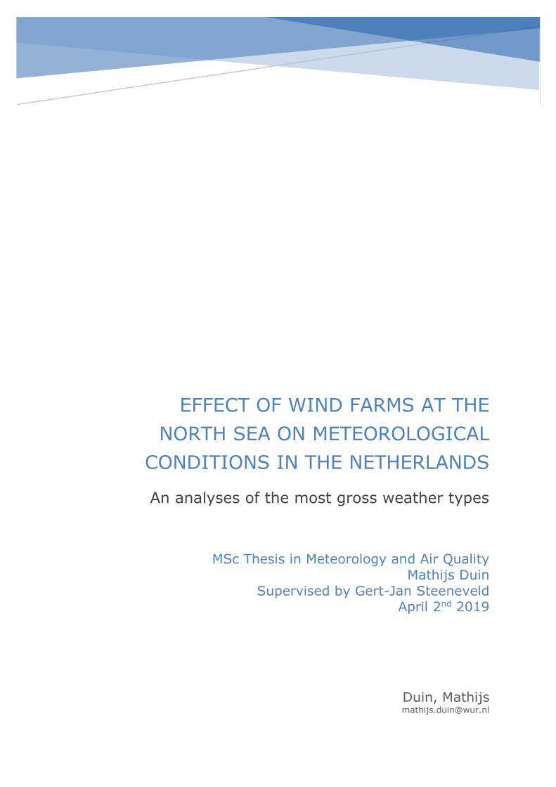
4.2.1. Wind speed In figure 8 the modelled climatological mean wind speed difference for the summer season is presented.

This climatological mean is defined by a weighted average over all 7 analysed summer season gross

weather types. In theory, in this climatological mean all wind directions should be averaged out. This is

also quite visible, because, on the contrary to the single map plots, the wakes of the wind farms do not

show a certain direction anymore but an average wind speed reduction in all sides. Especially at the wind

parks, the wind speed will be reduced by more than 1 m/s as well as in winter as in summer. An important

difference to notice is that in summer, the wind speed reduction wakes do not reach the Dutch mainland,

where in winter the wakes do. In general, the impacted wind speed area is larger than in summer. Also

between the wind parks, the wind speed will be reduced on average.

An important detail in wind reduction is that the wind only reduces over sea and in the first approximately

20 km in the coastal area. A possible explanation for this is, next to the fact that no wind parks are modelled

on land, the wind speed on land is already much lower. A wind speed reduction of 1 m/s is modelled on a

large part of the North Sea. For example, the magnitude of the average wind speed at K13 and

Europlatform is 8.25 m/s and 8.1 m/s respectively (Coelingh, Van Wijk, & Holtslag, 1996). Assuming a

similar mean wind speed at the rest of the North Sea, a wind speed reduction of about 1 m/s means a

wind speed reduction of over 10 % since P~U3 for wind speeds between 4 and approximately 10 m/s. This

wind speed reduction is of course also present at 100 m. This wind speed reduction at 100 m height (hub

height) is very important for wind energy production since the energy production correlates with the third

power of the wind speed at lower wind speeds. Important to mention is that at larger wind speeds, the

wind energy production does not correlate anymore with the third power wind speed. Here the correlation

is linear first, and not important anymore at wind speeds larger than 14 m/s. However, if we only apply a

third power to the wind speeds at hub height for both the control run and the wind farm run, we observe

a decrease in this third power number of 10 % in large parts of the western areas in the Netherlands

(figure 9). This decrease in wind speed power three is more than 20 % at the western and southern North

0,00

0,50

1,00

1,50

2,00

2,50

3,00

Win

d b

ias

(m/s

)Te

mp

erat

ure

bia

s (K

)Model RMS stations

RMS wind winter RMS wind summer

RMS temperature winter RMS temperature summer

12

Sea and North of the West Frisian islands. At the wind parks itself, this number decreases even more.

However, this is not relevant since these areas are already covered by wind farms in the model.

Figure 8 Modelled average change in 10-m wind speed in m/s due to installation of wind parks, left

winter, right summer.

Figure 9 Modelled percentage of change in wind speed to the power three at +/- 100 m height due to the installation of wind parks.

13

4.2.2. Temperature In figure 10 the modelled average temperature change is presented. In case of temperature change there

are two specifically interesting zones. First the provinces North-Holland and South-Holland, are expected

to experience a temperature reduction over 0.1 K in both winter and in summer. In winter, this temperature

decrease occurs in the entire northern and western area of the Netherlands. In winter, this temperature

decrease is quite consistent, and occurs in both daytime and night-time. In summer, this reduction is

mainly caused by daytime temperature reduction, while during the night, no large temperature reduction

is observed in this region. Another region with a summer temperature decrease is the coast of East Anglia.

This is because during two events, the summer south and the summer east circulation, the temperature

reduces with more than 0.2 K. Comparing this temperature change to the long term climate change, this

number is quite small. In De Bilt, the Netherlands, the average temperature has increased by 1.8 K

between 1903 and 2013. Since 1954, the temperature has increased with 1.4 K (KNMI, 2014). A decrease

in temperature by wind farms of 0.1-0.2 K looks minor, but this reduces actually 5 – 10 % of the

temperature increase in the last century to a magnitude between 1.2 and 1.3 K.

A controversial change in temperature happens in the summer in the Central Netherlands. In this region a

strong decrease in temperature is located next to a strong increase in temperature. There are mainly two

events contributing to this “wave” in temperature change; the summer southern circulation event and the

summer northern event. These two events have a large difference magnitude. There is no single conclusion

about the effect on the location of the wind farms.

Figure 10 Modelled change in average 2-m temperature in Kelvin. Left winter, right summer

14

4.2.3. Humidity When the wind farms are constructed, the humidity will decrease too (figure 11). This can be explained by

the increase in boundary-layer height above the wind parks. This boundary-layer height increase can be

explained by the increased turbulence due to turbine rotation (Frandsen et al., 2006). The reduction will

be the strongest in summer, but also in winter is a clear effect visible. The moisture content above the

windfarms reduces approximately 0.15 g/kg. In summer the effect is stronger, and the decrease in

humidity is also visible further from the wind farms. For example, Noord-Holland experiences a humidity

decrease of 0.1 g/kg.

Figure 11 Modelled change in 2-m average atmospheric moisture content in g/kg, left winter, right summer.

4.2.4. Precipitation For precipitation a much less clear effect is modelled (figure 12). The changes in precipitation presented

in the map are the change in modelled accumulated precipitation of all gross weather types in the presented

season. This means, the decrease is modelled over 56 days. For a yearly change in precipitation one needs

to multiply this number by approximately 6.75. In the climatological picture are some regions presented

with an increase in precipitation, and some regions with a decrease in precipitation. However, the patterns

are very irregular. Only some detail is visible in both pictures, and that is that above the wind farms the

precipitation increases. The largest areas with decrease in precipitation are located south-east of the wind

farms and the areas with the largest increase in precipitation are located at the wind farms.

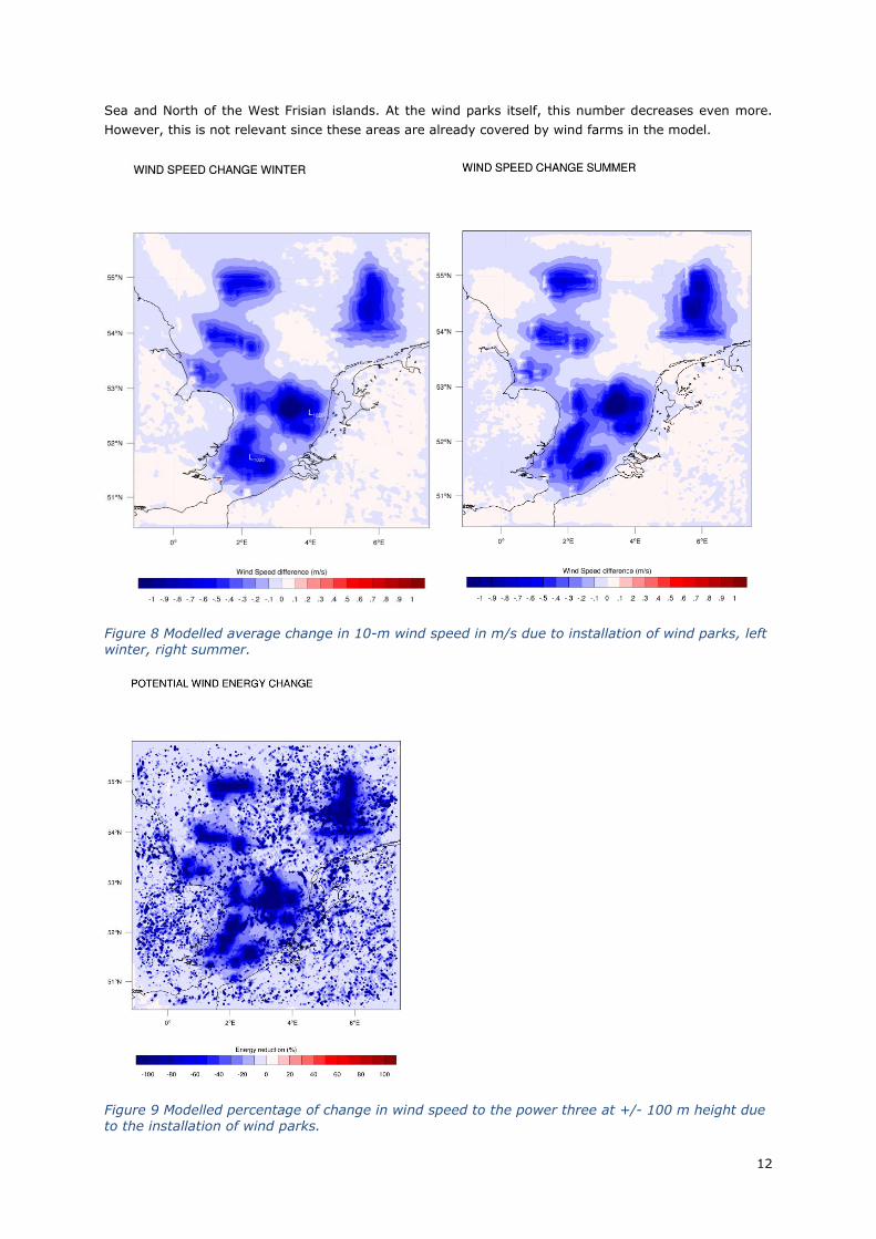
4.2.5. Solar radiation and clouds The change in precipitation is also supported by the radiation map (figure 13). Indeed, at the locations

with more precipitation, at which the wind farms are located, less net radiation will be received. A reduction

in radiation is actually only modelled in areas above large wind farms, not on small wind farms. This in

contrary to the effect of wind farms on humidity, where the humidity decreases above all wind farms of

each size significantly. In winter there is no clear effect, but in summer, the regions south-east and east

of the wind farms, including North and South-Holland will receive more radiation. In theory, this means

15

that these regions will get more suitable for solar energy. The largest decreases are above the existing

wind farms. Here a reduction of approximately 20 W/m2 can be expected. This corresponds to

approximately 10 %. The maximal increase in solar radiation averaged over 24 hours corresponds to an

increase of approximately 4 %. Note that the time over night is also included in the average and daylight

duration varies within the seisons. If we put this in a perspective of energy production, the western part

of the Netherlands and the North Sea will have slightly lower wind speeds, but a higher solar incoming

radiation.

Figure 12 idem, change in modelled cumulative precipitation in mm during simulated period (all simulations in the described season), left winter, right summer.

16

Figure 13 Modelled change in average surface shortwave-in radiation in W/m2, left winter, right summer. Note that the legend scale of these two figures differ.

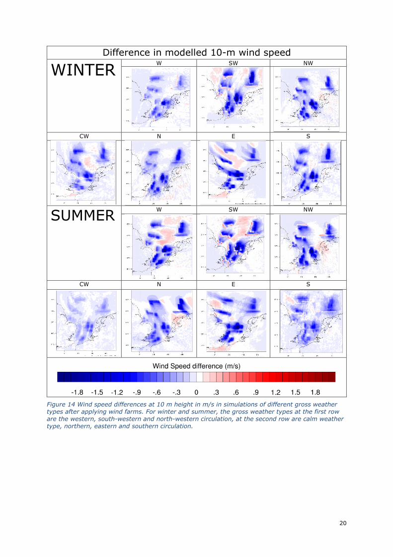
4.3. Individual cases The climatological outputs are based on the contribution of 7 gross weather types. In this section the

individual contribution of each gross weather type simulation to the climatological mean will be discussed.

4.3.1. Wind Speed During the westerly circulation in winter (figure 14), the downwind wind speed reduction exceeds 1 m/s

until the coast of North-Holland and South-Holland. During the north-westerly circulation (figure 14 Winter

NW) the wind speed reduction is similar. Also during this circulation, the wind speed reduction reaches the

Dutch coast. During the southern and south-westerly circulation (figure 14 Winter-S and -SW) the wind

speed reduction is downwind too. However, due to the direction of the wind, the wind speed reduction only

occurs at the North Sea. At the coastal and land areas no wind speed reduction occurs. Also, during the

northerly circulation (figure 14 Winter – N), the wind speed reduction area does not reach the Dutch coast,

this because the wind farms north of the Netherlands, are located at a large distance from the coast. For

the eastern wind (figure 14 Winter -E) the effect is different, but due to the probably stable atmosphere,

the wakes are very visible. The wakes are very far stretched and reach the coast of England. Between

these wakes of wind speed reduction, there are regions modelled with an average wind speed increase of

0.3 m/s. During the north-west circulation event, a similar effect occurs around the West Frisian islands.

During the calm weather event (figure 14 Winter-CW), there is wind speed reduction at the wind farms

and a local increase in wind speed in-between the wind farms. Another important detail in the wind speed

change prediction is the local increase in wind speed just upwind of the wind farm. During the westerly

circulation (figure 14 Winter-W) the reduction is not that strong with a magnitude of 0.3 m/s, but during

the south-west and north-west circulation (figure 14 Winter-NW and -SW) the wind speed increase upwind

of the wind farms is up to 0.5 m/s.

17

In summer, the patterns are quite similar as in winter. A difference is that during the westerly circulation

(figure 14 Summer -W), a wind speed increase region occurs with a magnitude of more than 0.3 m/s. The

entire coastal region of North and South-Holland is involved in the wind speed reduction. Along the coast,

the wind speed reduction is on average more than 0.3 m/s.

4.3.2. Humidity For the humidity the situation is totally not similar (figure 15). As already mentioned in the climatology

chapter, the humidity content decreases at the surface in almost the entire studied domain. For individual

cases, this is also true in winter, except for the southerly circulation (figure 15 Winter-SW). For this change,

no direct explanation is available, since the locations with humidity increase are not located downwind

from the wind farms, which means that in these regions no influence should be expected. In model terms,

the change in humidity can possible be explained by the modelled change in temperature in these regions.

If related to the validation, it is clear that the summer south circulation everywhere overestimates the

temperature, which could affect the atmospheric moisture concentrations in general. This could be a reason

that this model simulation does not agree with the other model simulations which give an overall humidity

decrease in winter.

On the contrary, in summer, for individual cases, the humidity at the surface increases in some situations.

This occurs for example in the summer northerly circulation in the middle of the Netherlands (figure 15

Summer -N). A possible explanation for this occurrence is a relocated squall line, because the precipitation,

temperature and radiation plots for this simulation has large changes in this location. Important to notice

is that this squall line does possible not have a correlation with the wind parks. In this simulation, the high

pressure areas have shifted northward and pressure is increased by 0.1 hPa in the north and decreased

by 0.1 hPa in the south. In the summer easterly circulation event (figure 15 Summer-E), the humidity

increases over land, but not over sea. This is quite suspicious, because this decrease in humidity is not

going parallel with an decrease in boundary-layer height. Neither the radiation or wind speed is changing

on average in these regions. The only explanation for this increase in humidity in coastal areas is the

increase in temperature. According to the Clausius-Clapeyron equation (August, 1828), air with a higher

temperature can contain a larger humidity. This explanation is supported by the fact that in areas (north

part of Noord-Holland), where the humidity decreases over land, the temperature also decreases. During

the south-west case (figure 15 Summer -SW), the humidity increases often directly downwind of the wind

farm. Also these areas experience a temperature decrease. When the calm weather event occurs in

summer, the situation is more divers. In general, the humidity decreases at the wind parks. On the

contrary, in areas between the wind parks, large areas occur with increasing humidity. Also here, the

temperature is higher in these areas with increased humidity.

4.3.3. Solar radiation and clouds As already mentioned in the climatology section, the shortwave downwelling radiation at the surface

decreases at the wind farm areas and increases east of these areas in summer (figure 16). The west coast

will receive more short wave-in radiation. This is mainly the case in the south-west and the west simulation

in summer (figure 16 Summer -SW and -W). In these two simulations the amount of short wave-in

radiation increases over the northern half of Noord-Holland. In other simulations the radiation amount does

not change that much or changes in a spread pattern.

4.3.4. Temperature

Winter

In figure 17, the change in temperature per simulation is presented. In winter, in the westerly circulation,

the temperature decreases with 0.1 K in a number of mainland areas in the Netherlands (figure 17 Winter-

W). The westerly circulation at the surface also reduces, which means that less warm marine air was

advected from the North Sea, which indeed reduces the humidity and temperature in the western part of

the Netherlands. This decrease in temperature is the strongest during night-time.

In the south-west winter simulation (figure 17 Winter-SW), the temperature increases at the wind farms

and downwind of the wind farms, basically in the areas where the humidity also increases. A possible

18

explanation is that the turbulence increases which means more heat from the sea surface is taken up. This

is supported because above land, the temperature does not increase and even decrease in the region of

Friesland. Also in this simulation, the temperature increases at locations with a boundary-layer height

increase. This increase in boundary-layer height is over 50 m at the wind farms, and up to 30 m between

the wind farms. In the region of Friesland, where the temperature decreases, the boundary-layer height

decreases by 20 m. Here the temperature decreases with 0.1 K. A change in boundary-layer height has

influence on the temperature since more warm upper air will be entrained when the boundary layer grows

(Tennekes & Driedonks, 1981).

In the north-west case (figure 17 Winter-NW), there is a lot spread in temperature change, both these

changes are of approximately 0.1 K. These changes correlate with the squall lines brought by the north-

westerly circulation (figure 18 Winter-NW). This is also the case during the northern circulation. These

squall lines are also recognisable on the radiation plot (figure 16 Winter-NW) and the humidity plot (figure

15 Winter-NW) of this simulation. These changes in squall lines could be a sign that weather systems are

relocated and shifted, which could have an effect on the surface temperature. In this case the changes in

temperature do not directly correlate with the presence of wind farms.

During the winter southerly wind simulation (figure 17 Winter-S), similar to the change in humidity (figure

15 Winter-S), the temperature changes over large areas without a certain explanation. However, these

changes in temperature correlate with changes in boundary-layer height and humidity in these regions. A

change in boundary-layer height has influence on the temperature since more warm upper air will be

entrained when the boundary layer grows (Tennekes & Driedonks, 1981). In the areas with the largest

temperature decrease, the boundary-layer height also decreases with approximately 30 m. In areas with

a temperature increase the boundary-layer height also increases up to 20 m.

In the eastern simulation (figure 17 Winter-E) the temperature decreases by 0.1 K, where downwind of

the wind farm the temperature often increase by 0.075 K. These temperature increase areas do not visually

correlate with a change in boundary-layer height downwind.

In the calm weather simulation (figure 17 Winter-CW) the temperature change varies over sea, but over

land, especially in nearly the entire part of the Netherlands, the temperature shows a strong decrease,

locally over 0.25 K. On the contrary, over sea, especially at wind parks, the temperature increases with

0.15 K. The temperature decreases in areas with a lower boundary-layer height and higher wind speed,

where the areas with a higher boundary-layer height and strongly reduced wind speeds experience a higher

temperature. Over land, the temperature decrease only correlates with the boundary-layer height. Here

the boundary-layer height decreases by 20 m on average. Important to mention is that during high

pressure situations, the wind speed is often below 4 m/s, which means that the wind turbines are not in

practise. In this simulation, the strongest increases are during daytime, and the strongest decreases at

night-time.

Summer

In the westerly circulation in summer there is a different pattern than in winter (figure 17 Summer-W).

The areas downwind of the wind farms, mostly at the sea, get a higher temperature of 0.1 K, dryer

atmosphere and a higher boundary-layer height. At the wind farms itself the temperature does not

increase, probably due to a reduction in radiation (increase of clouds) simultaneous with an increase in

boundary-layer height. Probably this increase in temperature is due to an increase in radiation. This

statement is supported because this temperature increase is happening during daytime, locally by more

than 0.15 K. On the contrary, the temperature decreases strongly further at the mainland.

In the south-west summer circulation (figure 17 Summer-SW), the temperature upwind of the wind farms,

decreases downwind of the wind farms and increases in the Netherlands by more than 0.15 K, locally this

temperature increase is over 0.2 K. In the areas with the highest temperature increases the shortwave-in

radiation also strongly increases (figure 16 Summer-SW). This increase is the strongest during daytime,

but also present at night-time. The increase in temperature during the day goes parallel with a strong

19

decrease in humidity (figure 15 Summer-SW), equal to the decrease in humidity at the wind farms, and

an increase in shortwave radiation.

In the summer north-westerly simulation (figure 17 Summer-NW), similar to the winter simulation, there

is again a lot of spread in temperature change simultaneous changes in squall lines, but in general, it gets

cooler at the mainland and at the wind farms. Here the temperature decreases up at 0.075 K. At the land

surface the temperature change fluctuates, due to squall lines which is also in this simulation visible on

the precipitation map (figure 18 Summer-NW). This is also the case in the summer northerly circulation

(figure 17 Summer-N & figure 18 Summer-N). The summer north simulation simulates a lot of spread in

temperature change. This because there are usually a lot of squall lines which could change location. That

is also the case in this simulation, in the areas with a large temperature increase or decrease, also a large

change in precipitation and locally even a large increase in humidity occurs (figure 15 Summer-N).

In the summer calm weather event (figure 17 Summer-CW), there are both large areas at the North Sea

experiencing an increase or decrease up to 0.2 K. Over land there is a lot of spread. Important to mention

again is that calm weather situations, the wind speed is often below 4 m/s, which means that the wind

parks are not in practise. In this simulation, the strongest increases are during daytime, and the strongest

decreases at night-time.

In summer, during the easterly circulation (figure 17 Summer-E), the temperature decreases over several

wind farms, probably due to an increased exchange with the cooler sea surface. Also, at the Dutch

mainland, the temperature changes. Over land, there is a lot of spread in temperature change. This change

in temperature is quite unexpected, since the Dutch mainland is not located downwind of the wind farm.

For the southern part of the North Sea, the radiation decreases and the boundary-layer height increases

up to 20 m, which causes more surface fluxes, which means that more water, which is still cold at the

moment of simulation in April, gets evaporated and decreases the temperature. At the east coast of

England this effect is even stronger. Here an average increase of over 0.2 K occurs where it is only 0.1 K

at the southern part of the southern North Sea.

In the southerly circulation (figure 17 Summer-S), the temperature changes are very strong. Also here,

these changes can only partly be explained by a change in a squall line. Side note for this simulation is

that this is the simulation with the highest temperature error (figure 5).

4.3.5. Precipitation For precipitation, as already mentioned in the climatology, the precipitation in general increases at and

upwind of the wind farms, and decreases downwind of the wind farms (figure 18). Actually, due to the

probable replacement of squall lines, there is a lot of spread in the outcomes with large increases and

decreases on short distance difference.

20

Difference in modelled 10-m wind speed

WINTER

W SW NW

CW N E S

SUMMER W SW NW

CW N E S

Figure 14 Wind speed differences at 10 m height in m/s in simulations of different gross weather

types after applying wind farms. For winter and summer, the gross weather types at the first row are the western, south-western and north-western circulation, at the second row are calm weather type, northern, eastern and southern circulation.

21

Difference in modelled humidity at 2 m

WINTER

W SW NW

CW N E S

SUMMER W SW NW

CW N E S

Figure 15 Differences in modelled atmospheric moisture content at 2 m in g/kg in simulations of

different gross weather types after applying wind farms. For winter and summer, the gross weather types at the first row are the western, south-western and north-western circulation, at the second row are calm weather type, northern, eastern and southern circulation

22

Difference in modelled surface shortwave-in radiation

WINTER

W SW NW

CW N E S

SUMMER W SW NW

CW N E S

Figure 16 Modelled surface shortwave-in differences in W/m2 in simulations of different gross weather types after applying wind farms. For winter and summer, the gross weather types at the first row are the western, south-western and north-western circulation, at the second row are calm weather type, northern, eastern and southern circulation. The differences in axes are due to the differences in magnitude between radiation in winter and in summer.

23

Difference in modelled 2-m temperature

WINTER

W SW NW

CW N E S

SUMMER W SW NW

CW N E S

Figure 17 Modelled 2-m temperature differences in K in simulations of different gross weather

types after applying wind farms. For winter and summer, the gross weather types at the first row are the western, south-western and north-western circulation, at the second row are calm weather type, northern, eastern and southern circulation.

24

Difference in modelled precipitation

WINTER

W SW NW

CW N E S

SUMMER W SW NW

CW N E S

Figure 18 Differences in modelled precipitation in mm simulations of different gross weather types after applying wind farms. For winter and summer, the gross weather types at the first row are the western, south-western and north-western circulation, at the second row are calm weather type,

northern, eastern and southern Circulation. The precipitation is defined as the cumulative precipitation in one simulation (excluding spinup time)

25

5. Discussion In this section the weaknesses and recommendations of this study will be discussed. At first, the most

basic subject for discussion is the resolution. In this study a 3 x 3 km resolution, nested in a 15 x 15 km

resolution is used. A 3 x 3 km resolution is just sufficiently course or sufficiently fine to switch on the

convection parameterisation. In this study, the advection is still switched on, but of course, the atmospheric

moisture advection only has an influence on the precipitation and not on the wind speed. Possibly, after

this 3 km resolution, the 3 km resolution gives a lot of spread in precipitation differences. In the test case,

which was run on a 15 x 15 km resolution, this spread was out and gave a more clear result. On the

contrary, the small resolution of 3 km is needed to model the wind speed reduction and to resolve

convection (Pryor et al., 2018). This is in contrary to Tang et al. (2013) who stated that even a resolution

of 1.5 km can estimate biases in precipitation. The vertical resolution could even have been finer. According

to Lee & Lundquist (2017), the minimal vertical resolution should be 12 meters in the lowest 400 meters

of the atmosphere. This is not completely accomplished in my thesis.

Second, results of WRF are strongly dependent on which parameters are used in the MYNN scheme (Berg

et al., 2018). Also the definition of the turbine height is important. The definition of other turbine

parameters is very important too, especially for the parameters which have a strong influence on the

turbulent kinetic energy dissipation at hub height (Yang et al., 2017). They performed a sensitivity study

on the wind at turbine height based on different parameters in the MYNN scheme and found a significant

effect on vertical wind profiles.

The third aspect of discussion is the wind turbine parameterisation. Because only one type of turbines is

analysed, the choice of turbine types is very important. This because the modelled decreases in wind speed

are of course based on the power curve. Of course, the wind farm and wind turbine parameterisation aims

to be as representative as possible, but this study is based on future scenarios which are always insecure

to happen.

From the test case, we found that it makes sense in which domain or which domains the wind farms are

switched on. In this study, the wind farms are only switched on in the inner domain. It also was an option

to switch the wind farms on in both the inner domain and the outer domain. Advantage of this would be

that the situation is more realistic, because future wind farms will exist in both domains. Disadvantage of

this choice would be that WRF possibly calculates the wind parks twice, which is of course not realistic at

all. Summarized, this means that the largest lack in wind the turbine parameterisation and wind park

parameterisation in this study is that everything is based on one scenario. Due to computational costs, and

a different focus on this study which focusses on the effect of wind farms on climatology, only one scenario

is analysed. This brings us to a challenge for future research. Out of this study, the effect of different types

of wind turbines or different wind park scenarios, on the downwind meteorology can be studied.

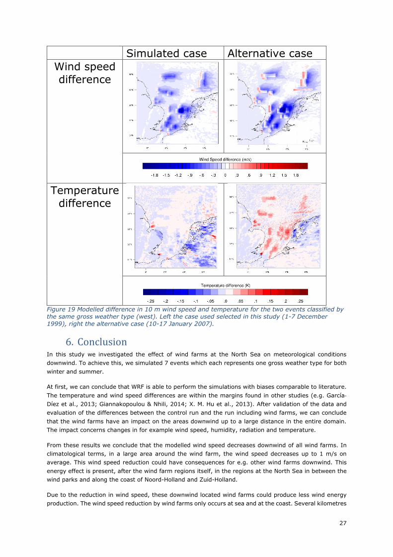
A fourth dilemma in this discussion is the case selection. In this study, the case selections strategy is

mostly based on Koopmans et al. (2015). Advantage of this selection method is the relatively low

computational coast (only 2*7*8 = 112 days) compared to for example a one year simulation. Another

advantage is that all common weather conditions which occur in this region over a longer time period are

represented. Disadvantage of this method of case selection is that there is variability between different

events which are still classified under the same gross weather type. To illustrate this difference, we

compared the selected winter west circulation with another event which is classified under the same gross

weather type. The case used in this study (1-8 December 1999) is an event which is classified as “westerly

cyclonic” in Werner & Gerstengarbe (2010). This circulation type is dominated by depressions which move

from west to east over Europe (Werner & Gerstengarbe, 2010). We compared this case with another

westerly circulation event in winter, occuring from January 10th until January 17th 2007, which also included

some days classified as “westerly anticyclonic”. A difference of this pattern is that the low pressure centre

is much further north and the Azoren High is much closer (Werner & Gerstengarbe, 2010). The differences

of these two events are presented in figure 19.

26

For wind speed the large-scale pattern between the simulated case and the alternative case is similar. The

surface wind speed reduction basically happens east of the wind farms until the Dutch coast. Even the

small zone with wind speed increase upwind of the windfarms is present. However, the magnitude of the

wind speed reduction is up to 0.5 m/s at the Dutch coast, which is much larger. Also, the wakes in the

alternative case are much more south-west north-east orientated, which is a sign for more south-westerly

wind.

This is also visible in the temperature graph. In both cases, the 2-m temperature decreases in the

Netherlands. However, the alternative case shows much more similarities with the south-western case of

this study (1-8 December 2000).

To solve the randomness of this selection method, multiple events, for example two or three events, can

be used to represent a certain gross weather type, especially when the gross weather type has a large

weight in the climatological average. Another solution could be to perform a one year simulation.

Advantage of a one year simulation would have been that simply one year would be simulated without any

interruptions. On the contrary to our simulation, nearly no spinup time would have been lost, where in our

simulations 14 days of spinup time are lost. The largest disadvantage of a long simulation of one year

would have been that one year, for example 2018, could be an exceptional year instead of a representative

year. To avoid this problem, the run could be performed for a climatological period, but regarding the

current computer capacity, that is not realistic when using this fine resolution which is used in this study.

From our model simulations we can conclude that wind farms could have a substantial influence on

downwind weather and even on downwind climate. We found several effects on wind, temperature,

precipitation, radiation and atmospheric moisture content. In case more wind farms will be constructed in

the future it could be useful to take these changes in weather into account with for example weather

predictions or climate scenarios. Also for future planned wind farms, it is, according to the results in this

study, useful to check if the wind at these projected wind farms is not too much disturbed by already

constructed wind farms upwind.

27

Simulated case Alternative case

Wind speed

difference

Temperature

difference

Figure 19 Modelled difference in 10 m wind speed and temperature for the two events classified by the same gross weather type (west). Left the case used selected in this study (1-7 December 1999), right the alternative case (10-17 January 2007).

6. Conclusion In this study we investigated the effect of wind farms at the North Sea on meteorological conditions

downwind. To achieve this, we simulated 7 events which each represents one gross weather type for both

winter and summer.

At first, we can conclude that WRF is able to perform the simulations with biases comparable to literature.

The temperature and wind speed differences are within the margins found in other studies (e.g. García‐

Díez et al., 2013; Giannakopoulou & Nhili, 2014; X. M. Hu et al., 2013). After validation of the data and

evaluation of the differences between the control run and the run including wind farms, we can conclude

that the wind farms have an impact on the areas downwind up to a large distance in the entire domain.

The impact concerns changes in for example wind speed, humidity, radiation and temperature.

From these results we conclude that the modelled wind speed decreases downwind of all wind farms. In

climatological terms, in a large area around the wind farm, the wind speed decreases up to 1 m/s on

average. This wind speed reduction could have consequences for e.g. other wind farms downwind. This

energy effect is present, after the wind farm regions itself, in the regions at the North Sea in between the

wind parks and along the coast of Noord-Holland and Zuid-Holland.

Due to the reduction in wind speed, these downwind located wind farms could produce less wind energy

production. The wind speed reduction by wind farms only occurs at sea and at the coast. Several kilometres

28

inland the wind speed reduction is less than 0.1 m/s, and at the coast of Noord-Holland and South-Holland,

the wind speed is reduced within 0.1 and 0.2 m/s in summer and less than 0.1 m/s in winter. For individual

cases, the wind speed change is different, but in general, the wind speed is of comparable magnitude of 2

m/s, but downwind of the wind farm.

Humidity decreases directly at the wind farm locations in both seasons summer and winter. The decrease

is up to 0.2 g/kg at the wind farms. At other locations in the domain, there is also reduction in humidity.

The magnitude of this decrease is in winter approximately 0.04 g/kg. In summer, the reduction is larger,

approximately 0.06 g/kg. Only Noord-Holland experiences a larger decrease, but this is caused by one

simulation event.

The temperature also changes. In summer, this change is not always clear, due to the contribution of some

gross weather type simulations which show a lot of spread. In winter, the conclusion is more clear. Large

parts of the Netherlands will experience a decrease in average 2-m temperature. This decrease is the

largest in the western part of the Netherlands, where the 2-m temperature in winter decreases with 0.1 K

on average.

References 4cOffshore. Global Offshore Renewable Map. Retrieved from https://www.4coffshore.com/offshorewind/

August, E. (1828). Ueber die Berechnung der Expansivkraft des Wasserdunstes. Annalen der Physik, 89(5), 122-137.

Berg, L. K., Liu, Y., Yang, B., Qian, Y., Olson, J., Pekour, M., . . . Hou, Z. (2018). Sensitivity of Turbine-Height Wind Speeds to Parameters in the Planetary Boundary-Layer Parametrization Used in the Weather Research and Forecasting Model: Extension to Wintertime Conditions. Boundary-Layer Meteorology, 1-12.

Bianchi, F. D., Battista, H., & Mantz, R. (2007). Kordesch, Wind Turbine Control Systems. In: Springer. Bijma, J. (2012). Nauwkeurigheid van operationele temperatuurmetingen, De Bilt, Netherlands: Technical

report; TR-328 Retrieved from http://bibliotheek.knmi.nl/knmipubTR/TR328.pdf

Coelingh, J., Van Wijk, A., & Holtslag, A. (1996). Analysis of wind speed observations over the North Sea. Journal of Wind Engineering and Industrial Aerodynamics, 61(1), 51-69.

Danish Wind Energy Association. (2003 June 1st ). Wind Speeds & Energy, The Power of the Wind: Cube of Wind Speed Retrieved from http://drømstørre.dk/wp-content/wind/miller/windpower%20web/en/tour/wres/enrspeed.htm

Desmond, C., Murphy, J., Blonk, L., & Haans, W. (2016). Description of an 8 MW reference wind turbine. Journal of Physics: Conference Series, 753. doi:10.1088/1742-6596/753/9/092013

Fitch, A. C., Olson, J. B., & Lundquist, J. K. (2013). Parameterization of Wind Farms in Climate Models. Journal of Climate, 26(17), 6439-6458. doi:10.1175/Jcli-D-12-00376.1

Fitch, A. C., Olson, J. B., Lundquist, J. K., Dudhia, J., Gupta, A. K., Michalakes, J., & Barstad, I. (2012). Local and Mesoscale Impacts of Wind Farms as Parameterized in a Mesoscale NWP Model. Monthly Weather Review, 140(9), 3017-3038. doi:10.1175/Mwr-D-11-00352.1

Frandsen, S., Barthelmie, R., Pryor, S., Rathmann, O., Larsen, S., Højstrup, J., & Thøgersen, M. (2006). Analytical modelling of wind speed deficit in large offshore wind farms. Wind Energy: An International Journal for Progress and Applications in Wind Power Conversion Technology, 9(1‐2), 39-53.

García‐Díez, M., Fernández, J., Fita, L., & Yagüe, C. (2013). Seasonal dependence of WRF model biases and

sensitivity to PBL schemes over Europe. Quarterly Journal of the Royal Meteorological Society, 139(671), 501-514.

Giannakopoulou, E. M., & Nhili, R. (2014). WRF Model Methodology for Offshore Wind Energy Applications. Advances in Meteorology. doi:Artn 3198 1910.1155/2014/319819

Global Wind Energy Council. (2017). Global Wind Report. Retrieved from http://files.gwec.net/files/GWR2017.pdf

Grabau, J. (1987). Klimaschwankungen und Großwetterlagen in Mitteleuropa seit 1881. Geographica Helvetica. Geographica Helvetica, 1, 35-40.

Hong, S.-Y., & Lim, J.-O. (2006). The WRF Single-Moment 6-Class Microphysics Scheme (WSM6). Journal of the Korean Meteorological Society, 42(2), 129-151.

Hu, X.-M., Nielsen-Gammon, J. W., & Zhang, F. (2010). Evaluation of three planetary boundary layer schemes in the WRF model. Journal of Applied Meteorology and Climatology, 49(9), 1831-1844.

Hu, X. M., Klein, P. M., & Xue, M. (2013). Evaluation of the updated YSU planetary boundary layer scheme within WRF for wind resource and air quality assessments. Journal of Geophysical Research: Atmospheres, 118(18), 10,490-410,505.

Jimenez, P. A., Navarro, J., Palomares, A. M., & Dudhia, J. (2015). Mesoscale modeling of offshore wind turbine wakes at the wind farm resolving scale: a composite-based analysis with the Weather Research and Forecasting model over Horns Rev. Wind Energy, 18(3), 559-566. doi:10.1002/we.1708

29

KNMI. Uurgegevens van het weer in Nederland. Retrieved from https://www.knmi.nl/nederland-nu/klimatologie/uurgegevens

KNMI. Uurgegevens van Noordzee stations. Retrieved from https://www.knmi.nl/nederland-nu/klimatologie/uurgegevens_Noordzee

KNMI. (2001). Handboek Waarnemingen. In (Vol. March 2001). De Bilt, Netherlands. KNMI. (2014). KNMI’14 climate scenarios for the Netherlands; A guide for professionals in climate adaptation.

Retrieved from KNMI, De Bilt, The Netherlands: http://www.climatescenarios.nl/images/Brochure_KNMI14_EN_2015.pdf

Koopmans, S., Theeuwes, N. E., Steeneveld, G. J., & Holtslag, A. A. M. (2015). Modelling the influence of urbanization on the 20th century temperature record of weather station De Bilt (The Netherlands). International Journal of Climatology, 35(8), 1732-1748. doi:10.1002/joc.4087

Lauridsen, M. J., & Ancell, B. C. (2018). Nonlocal Inadvertent Weather Modification Associated with Wind Farms in the Central United States. Advances in Meteorology. doi:Artn 2469683 10.1155/2018/2469683

Lee, J. C. Y., & Lundquist, J. K. (2017). Evaluation of the wind farm parameterization in the Weather Research and Forecasting model (version 3.8.1) with meteorological and turbine power data. Geoscientific Model Development, 10(11), 4229-4244. doi:10.5194/gmd-10-4229-2017

Ministerie van Economische Zaken en Klimaat. (2018). Kabinet maakt plannen bekend voor windparken op zee 2024-2030. Retrieved from https://www.rijksoverheid.nl/onderwerpen/duurzame-energie/nieuws/2018/03/27/kabinet-maakt-plannen-bekend-voor-windparken-op-zee-2024-2030

Ministerie van Economische Zaken en Ministerie van Volkshuisvesting en Milieubeheer. Rijksoverheid stimuleert duurzame energie. Retrieved from https://www.rijksoverheid.nl/onderwerpen/duurzame-energie/meer-duurzame-energie-in-de-toekomst

Platis, A., Siedersleben, S. K., Bange, J., Lampert, A., Barfuss, K., Hankers, R., . . . Emeis, S. (2018). First in situ evidence of wakes in the far field behind offshore wind farms. Scientific Reports, 8. doi:ARTN 2163 10.1038/s41598-018-20389-y

Pryor, S. C., Barthelmie, R. J., Hahmann, A., Shepherd, T. J., & Volker, P. (2018). Downstream effects from contemporary wind turbine deployments. Journal of Physics: Conference Series, 1037. doi:10.1088/1742-6596/1037/7/072010

Skamarock, W. C., Klemp, J. B., Dudhia, J., Gill, D. O., Barker, D. M., Duda, M. G., . . . Powers, J. G. (2008). A description of the Advanced Research WRF Version 3. NCAR technical note, Mesoscale and Microscale Meteorology Division

Slawsky, L. M., Zhou, L. M., Roy, S. B., Xia, G., Vuille, M., & Harris, R. A. (2015). Observed Thermal Impacts of Wind Farms Over Northern Illinois. Sensors, 15(7), 14981-15005. doi:10.3390/s150714981

Sun, H. W., Luo, Y., Zhao, Z. C., & Chang, R. (2018). The Impacts of Chinese Wind Farms on Climate. Journal of Geophysical Research-Atmospheres, 123(10), 5177-5187. doi:10.1029/2017jd028028

Tang, Y. M., Lean, H. W., & Bornemann, J. (2013). The benefits of the Met Office variable resolution NWP model for forecasting convection. Meteorological Applications, 20(4), 417-426. doi:10.1002/met.1300

Tennekes, H., & Driedonks, A. (1981). Basic entrainment equations for the atmospheric boundary layer. Boundary-Layer Meteorology, 20(4), 515-531.

Tom Remy, A. M. (2018, February 2018). Offshore Wind in Europe. Key trends and statistics 2017. Retrieved from https://windeurope.org/wp-content/uploads/files/about-wind/statistics/WindEurope-Annual-Offshore-Statistics-2017.pdf

Vautard, R., Thais, F., Tobin, I., Breon, F. M., de Lavergne, J. G. D., Colette, A., . . . Ruti, P. M. (2014). Regional climate model simulations indicate limited climatic impacts by operational and planned European wind farms. Nature Communications, 5. doi:ARTN 319610.1038/ncomms4196

Werner, P., & Gerstengarbe, F. (2010). Katalog der Grosswetterlagen Europas (1881–2009). Retrieved from Potsdam, Germany: https://research.fit.edu/media/site-specific/researchfitedu/coast-climate-adaptation-library/europe/germany-amp-poland/Werner--Gerstengarbe.-2010.-Synoptic-Weather-Documents-1881-2009-[DEU].pdf

WINDPOWER. TEN of the Biggest Turbines. Wind Power Monthly. Retrieved from https://www.windpowermonthly.com/10-biggest-turbines

Xia, G., & Zhou, L. M. (2017). Detecting Wind Farm Impacts on Local Vegetation Growth in Texas and Illinois Using MODIS Vegetation Greenness Measurements. Remote Sensing, 9(7). doi:ARTN 698 10.3390/rs9070698

Yang, B., Qian, Y., Berg, L. K., Ma, P.-L., Wharton, S., Bulaevskaya, V., . . . Shaw, W. J. (2017). Sensitivity of turbine-height wind speeds to parameters in planetary boundary-layer and surface-layer schemes in the weather research and forecasting model. Boundary-Layer Meteorology, 162(1), 117-142.

Yuan, R. Y., Ji, W. J., Luo, K., Wang, J. W., Zhang, S. X., Wang, Q., . . . Cen, K. F. (2017). Coupled wind farm parameterization with a mesoscale model for simulations of an onshore wind farm. Applied Energy, 206, 113-125. doi:10.1016/j.apenergy.2017.08.018

Zhou, L. M., Tian, Y. H., Roy, S. B., Thorncroft, C., Bosart, L. F., & Hu, Y. L. (2012). Impacts of wind farms on land surface temperature. Nature Climate Change, 2(7), 539-543. doi:10.1038/Nclimate1505

30

Acknowledgements I would like to thank the ECMWF for making available the ECMWF reanalyses.

Appendix

namelist.wps

max_dom = 2, parent_grid_ratio = 1, 5, i_parent_start = 1, 62,

j_parent_start = 1, 56, number of parent domain cells = 150 x 150 number of nested domain cells = 201, 201, parent domain = 15000 x 15000 m

nested domain = 3000 x 3000 m

ref_lat = 53.10,

ref_lon = 1.75,

truelat1 = 53.10,

truelat2 = 1.75,

stand_lon = 1.75,

namelist.input (as far as not mentioned in previous namelist)

number of vertical levels = 41

parent_grid_ratio = 1, 5,

parent_time_step_ratio = 1, 5,

eta_levels = 1.000, 0.998, 0.996, 0.994, 0.992, 0.990, 0.988, 0.984, 0.980,

0.976, 0.972, 0.968, 0.964, 0.960, 0.956, 0.952, 0.946, 0.940, 0.930, 0.920, 0.910, 0.900,

0.890, 0.880, 0.870, 0.860, 0.850, 0.825,

0.800, 0.750, 0.700, 0.600, 0.500,

0.400, 0.300, 0.200, 0.10, 0.048,

0.029, 0.014, 0.000,

mp_physics = 6, 6,

bl_pbl_physics = 5, 5,

moist_adv_opt = 1, 1,

windfarm_opt = 0, 1, ; in case of wind farm parameterisation switched on