Effective Component Tuning in a Diesel Engine Model Using

EFFECTIVE COMPONENT TUNING IN A DIESEL ENGINE MODEL USINGSENSITIVITY ANALYSIS

Rasoul Salehi∗Mechanical EngineeringUniversity of Michigan

Ann Arbor, Michigan, 48109Email: [email protected]

Anna StefanopoulouMechanical EngineeringUniversity of Michigan

Ann Arbor, Michigan, 48109Email: [email protected]

ABSTRACT

Error propagation and accumulation is a common problemfor system level engine modeling at which individually modeledcomponents are connected to form a complete engine model. En-gines with exhaust gas recirculation (EGR) and turbocharginghave components connected in a feedback configuration (the ex-haust conditions affect the intake and the intake, consequently,affects the exhaust), thus they have a challenging model tuningprocess. This paper presents a systematic procedure for effectivetuning of an engine air-charge path model to improve accuracy atthe system level as well as reducing the computational complex-ity of tuning a large set of components. Based on using sensitivityanalysis, the presented procedure is used to inspect which com-ponent influences more a set of selected outputs in a model withhigh degree of freedom caused by many parameters of differentcomponents. After selecting the influential component, which isthe turbocharger in this study, further tuning is applied to pa-rameters in the component to increase the overall accuracy ofthe complete engine model. The corrections applied to the air-charge path model of a 6 cylinder 13L heavy duty diesel enginewith EGR and twin-scroll turbocharger was shown to effectivelyimprove the model accuracy.

∗Address all correspondence to this author.

NOMENCLATUREVARIABLESA Area (m2) Cp Heat capacity (J/kg/K)F Burned gas fraction (-) I Inertia (kg.m2)m Mass flow rate (kg/sec) M Torque (N.m)P Pressure (Pa) PR Pressure ratio (-)PW Power (W) T Temperature (K)R Gas constant (J/kg/K) r Comp. wheel radius (m)η Efficiency (-) ρ Density (kg/m3)ω Speed (RPM) γ Ratio of Cp/Cv (-)

SUBSCRIPTSc Compressor corr Correcteddst Downstream turbine e Engineeff Effective EGR Exh. gas recirculationeml Large scroll exh. man. ems Small scroll exh. man.im Intake manifold tc Turbochargert Turbine upc Upstream compressorupt Upstream turbine WG Wastegate

INTRODUCTIONControl and monitoring strategies in modern engine control

unites (ECUs) require use of many physical engine variables.The measurement cost or/and the sensibility of measuring a vari-able at harsh operating conditions of an internal combustion en-gine limits utilizing sensors on a production engine. Thereforeimplementation of engine models inside the ECU, instead of ad-dition of sensors, has been a common interest for engine man-ufacturers. The modeling work can be as simple as simulating

DSCC2015-9729

1 Copyright © 2015 by ASME

Proceedings of the ASME 2015 Dynamic Systems and Control Conference DSCC2015

October 28-30, 2015, Columbus, Ohio, USA

Downloaded From: http://proceedings.asmedigitalcollection.asme.org/ on 03/21/2016 Terms of Use: http://www.asme.org/about-asme/terms-of-use

pressure drop over the air filter [1] or as complicated as simulat-ing engine’s pollution gas and the emission system [2, 3]. What-ever the model is, a general approach in many developed enginemodels is physics-based modeling. The development of physicalengine models usually follows two steps. The first step, calledcomponent level modeling in this paper, comprises modeling in-dividual components based on their inputs and outputs measuredat steady state operating conditions. The second step is a systemlevel modeling at which all individual steady-state componentmodels are connected to form a complete engine model. When acomplete engine model (i.e. a system level model) is formed byconnecting models of individual components, the final accuracyreduces due to reasons such as error accumulation/propagationor mismatch between conditions of data collection for compo-nent level modeling and system level model verification (e.g. gasbench conditions used to provide a turbocharger map and condi-tions on an engine [4]). Therefore an overall parameter tuning atthe system level is required to improve the final performance ofthe complete engine model.

There are many candidates of parameters and components ina complete engine model to be considered in the final tuning pro-cess. To reduce the number of the candidates, this paper presentsa systematic methodology based on sensitivity analysis (SA) todetermine the major component influencing the complete enginemodel. Sensitivity analysis determines how selected model out-puts are affected by a small deviation in an individual compo-nent’s output. Then a metric is used to quantify the importance ofcomponents based on applying the principle component analysisto the sensitivity matrix. When the major influencing componentis detected, a fine tuning process is applied to that componentwhich improves performance of the engine model in predictingmeasured outputs.

DIESEL ENGINE MODEL

A control-oriented model of the air path of a 13 liters 6-cylinder heavy duty diesel engine, represented by the schematicin Fig. 1, is presented. The considered engine is equipped withan asymmetric twin-scroll turbine which has benefit in increas-ing exhaust gas recirculation (EGR) while keeping low the backpressure and smoke by mitigating long delays from the EGRpath. The engine is also equipped with a wastegate valve, whichbypasses the large scroll avoiding over-boosting and reducing thepumping loss.

Model development for this engine has two steps. The firststep is the component level where parameters to individuallymodel each component is estimated. At the system level, whichis the second step, all components are connected and final struc-ture of the complete engine model is formed. The following sub-sections describe each step respectively.

FIGURE 1: Schematic of the twin-scroll heavy duty diesel en-gine.

Component Level ModelingFor the engine schematically shown in Fig. 1, all compo-

nents (namely: engine block, turbocharger, intercooler, EGR andwastegate) are modeled individually. Inputs and outputs of eachcomponent are measured explicitly (except for the wastegate andEGR where their output flows are estimated). The components’models are mainly from the work presented in [5] with few re-estimation of parameters given that the engine considered hereis a different model year and has a smaller level of asymmetryin the turbine scroll. Since the turbocharger, EGR and waste-gate will be discussed further in later sections of the paper, theirmodels are presented briefly here.

The compressor map provided by the turbo supplier is themain data source for modeling its flow and efficiency at steadystate points. Two non-dimensional parameters are defined, thehead parameter (Ψ) and the flow parameter (Φ) [6] which areused to create a Φ−Ψ relation at each compressor speed using apolynomial regression. Then the compressor flow and efficiencycan be calculated as:

mc,map = θc ∗πr3ρωtc f1(Ψ) (1)

ηc = f2(Ψ) (2)

where r, ρ, ωtc are the compressor wheel radius, the inlet airdensity, the turbo speed and f1 and f2 come from regressionscorrelating Ψ−Φ and Ψ−η , respectively. The regression co-efficients are calculated by interpolating polynomial coefficientsindividually found at each compressor rotational speed [7]. Theparameter θc is introduced here to mathematically apply pertur-bations to the compressor flow as required by the sensitivity anal-ysis. The twin-scroll turbine flow is simulated as a function of thescrolls pressure ratio ( Pdst

Peml, Pdst

Pems) and the turbo shaft speed (ωtc).

The parametric model for the turbine flow can be found withgood accuracy using test with closed wastegate at the engine test



bench, unlike the compressor for which the high interaction be-tween the compressor variables (pressure ratio, speed and flow)implies using its characteristic map. The turbine efficiency iscalculated by creating a balance between the compressor and theturbine powers:

ηt =PWc

mtTuptCp(1− PdstPupt

γ/γ−1)

(3)

The turbine efficiency calculated from Eq. 3 takes values in therange of [.7− .8] and it can effectively be approximated as a con-stant [5]. The EGR flow is modeled using the standard isentropicorifice flow model as:

mEGR = θEGR ∗Ae f f ,EGRPems√RTems

F(PR), PR =Pim

Pems(4)

in which the parameter θEGR again is a mathematical param-eter defined to facilitate implementing the sensitivity analysiswithin the simulation. The effective area in Eq. 4, Ae f f ,EGR =gEGR(uEGR,ωe,PR), is a function of ECU command, uEGR, andalso pressure ratio and engine speed which are included to ac-count for the pulsation effects. The same isentropic orifice modelis used to simulate the WG flow rate:

mWG = θWG ∗Ae f f ,WG(xWG)Peml√RTeml

F(PR), PR =Pim

Peml(5)

where θWG is the parameter for the sensitivity analysis andxWG = gWG(uWG,Peml ,Pdst) is the wastegate displacement takenfrom the wastegate mechanism force balance [5].

The performance of the components’ models are presentedin Fig. 2. Figure 2-a,b compares the regression models to the datafrom the compressor map and in Fig. 2-c,d the modeled waste-gate and EGR mass flow rates are compared to their correspond-ing estimated values collected from tests at a highly instrumentedengine test bench [5]. As the plot shows, for most of the operat-ing points, there is good agreement (within a 10% error bound)between the modeled and measured data.

System Level ModelingThe complete engine model (shown schematically in Fig. 3)

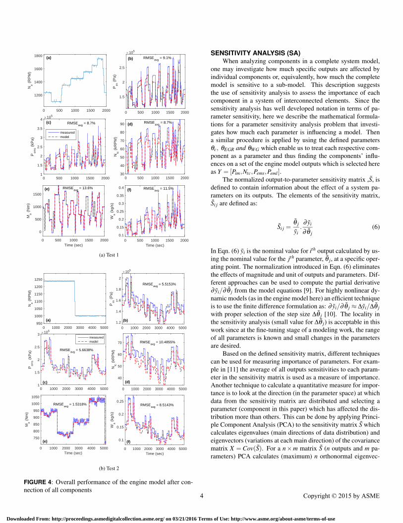
is formed by connecting individual components described in theformer subsection along with dynamical models for pressure(Pim, Pems, Peml , Pdst ), air fractions (Fim, Fem) and the turbochargerspeed (ωtc) as presented in [5]. Moreover, a temperature dynami-cal model has been augmented to the airflow dynamics to accountfor heat accumulation in the engine body [8] which improves theengine model capability to follow very slow dynamics observedin the measured data. The final performance of the complete

FIGURE 2: A summery of modeling results at the componentlevel

FIGURE 3: Overview of the complete engine model, its inputsand selected outputs

model is presented in Fig. 4. As plotted the general trend of theengine model follows that of the measurements. However, steadystate offset at different points is clearly observed. The averagedroot mean square (RMSEavg) in Fig. 4 is defined as the conven-tional RMSE divided by the average of measured data over theentire time window at each test. To remove the offset, a param-eter fine-tuning is required. The question is which componentshave the most influence and should be tuned. This is decidedusing the sensitivity analysis as described in the next section.



0 500 1000 1500 2000

Ne (

RP

M)

1200

1400

1600

1800 (a)

0 500 1000 1500 2000P

im (

Pa)

×105

1.5

2

2.5

RMSEavg

= 9.1%(b)

0 500 1000 1500 2000

Pem

s (kP

a)

×105

1

1.5

2

2.5

3

3.5

4RMSE

avg = 8.7%(c)

measuredmodel

0 500 1000 1500 2000

Ntc

(kR

PM

)

30

40

50

60

70

80

90 RMSEavg

= 8.7%(d)

Time (sec)0 500 1000 1500 2000

Me (

Nm

)

0

500

1000

1500

RMSEavg

= 13.6%(e)

Time (sec)0 500 1000 1500 2000

Wa (

kg/s

)

0.1

0.15

0.2

0.25

0.3

0.35

0.4 RMSEavg

= 11.5%(f)

(a) Test 1

0 1000 2000 3000 4000 5000

Ne (

RP

M)

950

1000

1050

1100

1150

1200

1250

(a)

0 1000 2000 3000 4000 5000

Pim

(P

a)

×105

1.2

1.4

1.6

1.8

2

RMSEavg

= 5.5153%

(b)

0 1000 2000 3000 4000 5000

Pem

s (kP

a)

×105

1

1.5

2

2.5

3

RMSEavg

= 5.6638%

(c)

measuredmodel

0 1000 2000 3000 4000 5000

Ntc

(kR

PM

)

40

50

60

70 RMSEavg

= 10.4855%

(d)

Time (sec)0 1000 2000 3000 4000 5000

Me (

Nm

)

750

800

850

900

950

1000

1050

RMSEavg

= 1.5318%

(e)

Time (sec)0 1000 2000 3000 4000 5000

Wa (

kg/s

)

0.1

0.15

0.2

0.25RMSE

avg = 8.5143%

(f)

(b) Test 2

FIGURE 4: Overall performance of the engine model after con-nection of all components

SENSITIVITY ANALYSIS (SA)When analyzing components in a complete system model,

one may investigate how much specific outputs are affected byindividual components or, equivalently, how much the completemodel is sensitive to a sub-model. This description suggeststhe use of sensitivity analysis to assess the importance of eachcomponent in a system of interconnected elements. Since thesensitivity analysis has well developed notation in terms of pa-rameter sensitivity, here we describe the mathematical formula-tions for a parameter sensitivity analysis problem that investi-gates how much each parameter is influencing a model. Thena similar procedure is applied by using the defined parametersθc, θEGR and θWG which enable us to treat each respective com-ponent as a parameter and thus finding the components’ influ-ences on a set of the engine model outputs which is selected hereas Y = [Pim,Ntc,Pems,Peml ].

The normalized output-to-parameter sensitivity matrix ,S, isdefined to contain information about the effect of a system pa-rameters on its outputs. The elements of the sensitivity matrix,Si j are defined as:

Si j =θ j

yi.

∂ yi

∂ θ j(6)

In Eqn. (6) yi is the nominal value for ith output calculated by us-ing the nominal value for the jth parameter, θ j, at a specific oper-ating point. The normalization introduced in Eqn. (6) eliminatesthe effects of magnitude and unit of outputs and parameters. Dif-ferent approaches can be used to compute the partial derivative∂ yi/∂ θ j from the model equations [9]. For highly nonlinear dy-namic models (as in the engine model here) an efficient techniqueis to use the finite difference formulation as: ∂ yi/∂ θ j ≈ ∆yi/∆θ jwith proper selection of the step size ∆θ j [10]. The locality inthe sensitivity analysis (small value for ∆θ j) is acceptable in thiswork since at the fine-tuning stage of a modeling work, the rangeof all parameters is known and small changes in the parametersare desired.

Based on the defined sensitivity matrix, different techniquescan be used for measuring importance of parameters. For exam-ple in [11] the average of all outputs sensitivities to each param-eter in the sensitivity matrix is used as a measure of importance.Another technique to calculate a quantitative measure for impor-tance is to look at the direction (in the parameter space) at whichdata from the sensitivity matrix are distributed and selecting aparameter (component in this paper) which has affected the dis-tribution more than others. This can be done by applying Princi-ple Component Analysis (PCA) to the sensitivity matrix S whichcalculates eigenvalues (main directions of data distribution) andeigenvectors (variations at each main direction) of the covariancematrix X = Cov(S). For a n×m matrix S (n outputs and m pa-rameters) PCA calculates (maximum) n orthonormal eigenvec-



tors in a m-dimensional space. The first eigenvector is the maindirection (in the m-dimensional space) at which data of S are dis-tributed. Therefor the weight of each element in an eigenvectorshows how much the corresponding parameter has contributed todata alignment in that direction [12].

The eigenvectors, [C1i, ...,C ji, ...,Cmi]T , and eigenvalues, λi,

from PCA of S are used to calculate the following importancemeasure for the j th parameter [13]:

µ j =

n∑

i=1|λiC ji|

n∑

i=1|λi|

(7)

with 0≤ µ j ≤ 1. As the numerator in Eqn. 7 suggests, the impor-tance of each parameter in a principle direction, C ji, is multipliedby the direction’s importance, λi. Since elements of S representdeviation of outputs due to perturbation in parameters, thus themeasure, µ j, shows how much perturbing the jth parameter hascontributed to deviation in the vector of outputs Y .

The importance measure introduced in Eqn. 7 for parameteranalysis is extended here to detect effectiveness of each com-ponent (instead of parameters) on the model outputs within thefollowing implementation procedure.

Implementation Procedure for SA

1- Select the outputs, components and design an operating pro-cedure. This procedure should allow all components (andtheir outputs) to be practiced in their effective range. Then,simulate the model without perturbing outputs of any com-ponent. This provides the base line (nominal) data.

2- Select a step size for perturbation in components outputs.The step size should be selected properly to estimate the par-tial derivative term in Eqn. 6 with finite differences. Perturbthe output of one component by the step size and run themodel. Use Eqn. 6 to calculate the first column of the sensi-tivity matrix. Repeat this step for all desired components.

3- Run PCA for the sensitivity matrix derived at the last stepand then use Eqn. 7 to calculate the importance measure foreach component.

Using SA For The Engine ModelThe 3-step proposed implementation procedure for SA is ap-

plied to the heavy duty diesel engine model described in section2. The first 2 steps calculate the sensitivity matrix and at step 3,the sensitivity of the engine model to each component is calcu-lated. The following describes details of applying the SA to theengine model.

Step1 The selected output vector is Y =[Pim, Ntc, Pems, Peml ]. Flow models for the compressor,

the EGR and wastegate are selected to be analyzed for theireffect on the output vector Y . To do this, the parameter vectorΘ = [θc,θEGR,θWG] with the initial value of Θ0 = [1,1,1] is usedto apply perturbations to the components’ flows. Two differenttest procedures were selected, one with major changes in theengine torque and engine speed and the other by major changesin the wastegate and EGR positions (Test 1 and Test 2 in Fig. 4respectively).

Step2 To estimate the derivative term in Eqn. 6 with afinite difference, ∆yi/∆θ j, the step size for ∆θ j should be prop-erly selected to ensure the required linearity condition ( whichneeds small ∆θ j) and to avoid treating noise and computation er-rors as sensitivities (which needs big ∆θ j) [10]. To select ∆θ j,the following criteria is calculated over a drive cycle time (T ) toevaluate the linearity:

L =

T∑

t=0(

θ j∆yiyi∆θ j

(t))−

T∑

t=0(

θ j∆yiyi∆θ j

)(t)+

(8)

where ((θ j∆yi)/(yi∆θ j))− is deviation in output yi due to a nega-tive perturbation (e.g. Θ= [1, .95,1] for 5% negative perturbationin EGR flow model) in the parameter θ j and ((θ j∆yi)/(yi∆θ j))+is due to a positive perturbation. Figure 5 shows L for Pim andωtc at different perturbation levels (defined as |θ j−1| ∗100) forperturbed EGR and compressor flows. As observed, a 5% pertur-bation has relatively linear influence while giving enough excita-tion to the outputs. Using the 5% perturbation for each element inthe parameter vector Θ, the sensitivity matrix is calculated fromEqn. 6

Step3 The importance measure µ j is calculated both withon-line and off-line calculations. At on-line approach, at eachsingle simulation step time the sensitivity matrix is calculatedfrom Eqn. 6 and, by using PCA, the corresponding µ j

′s are cal-culated. Figure 6 shows the results for both Test-1 and Test-2.As observed, the turbocharger has the main effect on the out-puts (though µθc is close to µθEGR in Test-1 which has trajecto-ries with high variations in engine speed and torque). The EGRcomes as the second influential component of the air-charge pathmodel and the wastegate shows the least influence on the model.One reason for higher EGR influence (compared to WG) is thatchanging the EGR affects both the turbine and engine flows di-rectly while the WG only has a direct effect on the turbine flow.

For off-line calculation of the importance measures, the sen-sitivity matrices calculated form Eqn. 6 at each step time are av-eraged over the whole range of a test procedure. In addition, theoperating points at which a component does not have any flow(such as when the wastegate is closed) were removed from the



Disturbance level, |θEGR

-1|*100 (%)0 5 10 15 20

L (

-)

1

1.2

1.4

1.6(a)

ωtc

Pems

Disturbance level, |θC

-1|*100 (%)0 5 10 15 20

L (

-)

0.7

0.8

0.9

1(b)

FIGURE 5: Linearity analysis with disturbance applied to theEGR and compressor flows

averaging procedure. Figure 7 shows the results for the off-lineanalysis. An interesting result from Fig 7 is that when the waste-gate and EGR are swept (i.e. Test-2) their effect is relativelycloser compared to the test (Test-1) at which there is no specificpattern for actuating (exciting) these two components. Thus, de-pending on the test cycle, each component may be found withdifferent importance for the model designer.

TUNING THE ORIGINAL MODELFrom the sensitivity analysis it was found that the compres-

sor flow used in the turbocharger dynamical model is the keyflow influencing the complete engine model. The compressorflow is a function of its pressure ratio and rotational speed whichboth have estimation errors as Fig. 4 shows. Even if the pres-sure ratio and the rotational speed are estimated accurately, therewould be deviations between the compressor characteristic mapdata provided by a turbo supplier and the one measured when itis integrated into an engine air path system. Therefore the tuningprocedure should reduce the estimation error for three variables;compressor pressure ratio, rotational speed and air flow. To doso, the turbocharger dynamical model is parameterized as:

Itcωtcωtc = α1mtTuptCp,t(1−Pdst

Pupt

(1−1/γt )

)−

[α2mc,map +α3]TupcCp,c(Pim

Pupc

(1−1/γc)

−1)

(9)

Time (sec)0 500 1000 1500 2000

Imp.

Mea

s., µ

(-)

0

0.2

0.4

0.6

0.8

1µθ,C

µθ,EGR

µθ,WG

(a) Test 1

Time (sec)0 1000 2000 3000 4000 5000

Imp.

Mea

s., µ

(-)

0

0.2

0.4

0.6

0.8

1µθ,C

µθ,EGR

µθ,WG

(b) Test 2

FIGURE 6: Importance measure for different components fromthe on-line analysis

θC

θEGR

θWG

Imp.

Mea

s., µ

(-)

0

0.2

0.4

0.6

0.8

(a) Test 1

θC

θEGR

θWG

Imp.

Mea

s., µ

(-)

0

0.2

0.4

0.6

0.8

(b) Test 2

FIGURE 7: Importance measure for different components fromthe off-line analysis

In Eqn. 9, α1 is included to cancel the inaccuracy in the tur-bocharger efficiency caused by pulsation and heat transfer whichhappen during the engine operation and α2 and α3 correct thecompressor flow model. An optimization problem can be definedto calculate these three parameters as the following:

[α1,α2,α3] = argminα1,α2,α3

||Pim,meas−Pim

Pim,meas||2 + ||

ωtc,meas−ωtc

ωtc,meas||2+

||mc,meas− mc

mc,meas||2

(10)



Estimated flow (kg/sec)0 0.1 0.2 0.3 0.4 0.5

Mea

sure

d fl

ow (

kg/s

ec)

0

0.1

0.2

0.3

0.4

0.5

10% boundary

(a)

Engine speed (RPM)1100 1300 1500 1700 1900

α1

1.02

1.04

1.06

1.08

1.1

1.12

(b)

FIGURE 8: (a) Comparison between measured and estimatedcompressor flow. (b) α1 as a function of the engine speed.

where Pim is the estimated intake manifold pressure from the fill-ing dynamics and

mc = α2mc,map +α3 (11)

It is difficult to solve the optimization problem for all three pa-rameters simultaneously from Eqn. 10 subjected to the nonlinearengine equations. Instead, a specific procedure is proposed hereto tune all three parameters within a 2-step solution as describedin the following.

Step1: Tuning the Compressor Flow ModelAt the first step, α2, α3 used to apply the bi-linear correction

to the compressor flow model were estimated using linear leastsquare method to remove the compressor flow error defined as:emc = mc,meas− ˆmc using measurements collected during the en-gine mapping tests. The compressor flow corrected by α2 = 0.9and α3 =−0.027 is compared to the measured air flow in Fig. 8-(a). As shown, the model matches the measured data within the10% accuracy bound as plotted.

Step2: Tuning the turbocharger efficiencyThe compressor model from Step1 assures that if Pim and ωtc

are estimated accurately, the compressor air flow from Eqn.11would be accurate as well. Therefore, the optimization problemdefined in Eqn. 10 is reduced to:

α1 = argminα1

||Pim,meas− Pim

Pim,meas||2 + ||

ωtc,meas− ωtc

ωtc,meas||2 (12)

Equation. 12 is solved numerically using the steepest descent al-gorithm over drive cycles different to what is shown in Fig. 4in which the engine speed was kept constant and calculated α1is tabulated as shown in Fig. 8-(b). Final results of the modelwith applied corrections to the turbocharger model are shown inFig. 9 within test procedures similar to those shown in Fig. 4.Compared to Fig. 4, both test cycles show noticeable accuracyimprovements for all variables except the engine torque. The rea-son for this observation is that in a diesel engine, torque is mainlyaffected by the amount of injected fuel [5].

CONCLUSIONA new methodology to detect main elements in a complete

engine model was presented in this paper. A heavy duty 6-cylinder engine model with high pressure EGR was developedat first. For the modeling, each component was modeled indi-vidually using data from steady state engine tests and then thecomplete engine model was formed by connecting componentmodels. Despite the fact that individual component models hadacceptable accuracy, noticeable offset from measured data wasobserved when the complete engine model was simulated. Tofurther tune the model, sensitivity analysis was used to deter-mine how much specific components affect the complete enginemodel and select the most influential one. This was done byprinciple component analysis of the sensitivity matrix and useof a measure for quantifying the importance. It was found thatthe turbocharger was the main component among selected ones.Moreover, the importance measure was found dependent on theselected test procedure by showing different levels of importancefor each selected component at different test procedures. Finaltuning was applied to the turbocharger model in a two step pro-cedure showed remarkable improvement of the complete enginemodel.

ACKNOWLEDGMENTThe authors would like to thank Dan Potter, Jasman S. Malik

and Peter Attema of Detroit Diesel Corporation (DDC) for theirtechnical advice. We also appreciate Michael Uchanski and De-jan Kihas of Honeywell for sharing their experiences in modeltuning from OnRAMP Design Suite. Funding for this work wasprovided by DDC.



(a) Test 1

(b) Test 2

FIGURE 9: Performance of the tuned engine model

REFERENCES[1] L. Guzzella, C.H. Onder, 2010 Introduction to Model-

ing and Control of Internal Combustion Engine Systems.,Springer, Berlin.

[2] A. Schilling, et al., 2006 Real-time model for the predictionof the NOx emissions in DI diesel engines., IEEE Interna-tional Conference on Control Applications.

[3] D. N. Tsinoglou, M. Weilenmann, 2009 A Simplied Three-Way Catalyst Model for Transient Hot-Mode Driving Cy-cles., Ind. Eng. Chem. Res. 48: 17721785.

[4] S. Marelli, M. Capobianco 2011 Steady and pulsating flowefficiency of a waste-gated turbocharger radial flow turbinefor automotive application, Energy 36(1): 459-465

[5] Hand M. J., et. al., 2013 Model and calibration of adiesel engine air path with an asymmetric twin scroll tur-bine.,ASME 2013 internal combustion engine conference.

[6] R. Salehi, et. al., 2014 Air Leak Detection for a Tur-bocharged SI Engine using Robust Estimation of the Tur-bocharger Dynamics, SAE Int. J. Passeng. Cars Electron.Electr. Syst. 7(1)

[7] J. E. Hadef, et. al., 2012 Physical-Based Algorithms for In-terpolation and Extrapolation of Turbocharger Data Maps,SAE Int. J. Engines 5(2): 363-378.

[8] L. Eriksson, 2002 Mean Value Models for Exhaust Sys-tem Temperatures., SAE world congress, Technical paper,2002-01-0374.

[9] A. Sandu, et al., 2003 Direct and adjoint sensitivity analy-sis of chemical kinetic systems with KPP: Part Itheory andsoftware tools., Atm. Env. 37(36): 5083-5096.

[10] D.J.W. DE Pauw and P. A. Vanrolleghem, 2006 Practicalaspects of sensitivity function approximation for dynamicmodels, Math. and Comp. Modelling of Dynamical Sys-tems 12(5): 395-414.

[11] S.R. Weijers and P. A. Vanrolleghem, 1997 A procedurefor selecting best identifiable parameters in calibrating ac-tivated sludge model no. 1 to full-scale plant data., WaterScience and Technology 36(5): 69-79.

[12] G.H. Dunteman, 1989 Principal component analysis(Quantitative applications in the social sciences), Sagepublications, inc.

[13] L. Rujun, et al., 2004 Selection of model parameters for off-line parameter estimation., IEEE Control Systems Technol-ogy, 12(3): 402-412.



Documents

Effective Component Tuning in a Diesel Engine Model Using