HAL Id: hal-03185532https://hal.inria.fr/hal-03185532v1

Preprint submitted on 30 Mar 2021 (v1), last revised 14 Apr 2021 (v2)

HAL is a multi-disciplinary open accessarchive for the deposit and dissemination of sci-entific research documents, whether they are pub-lished or not. The documents may come fromteaching and research institutions in France orabroad, or from public or private research centers.

L’archive ouverte pluridisciplinaire HAL, estdestinée au dépôt et à la diffusion de documentsscientifiques de niveau recherche, publiés ou non,émanant des établissements d’enseignement et derecherche français ou étrangers, des laboratoirespublics ou privés.

Effective Controllability Test for Fast Oscillating ControlSystems. Application to Solar Sailing

Alesia Herasimenka, Jean-Baptiste Caillau, Lamberto Dell’Elce, Jean-BaptistePomet

To cite this version:Alesia Herasimenka, Jean-Baptiste Caillau, Lamberto Dell’Elce, Jean-Baptiste Pomet. Effective Con-trollability Test for Fast Oscillating Control Systems. Application to Solar Sailing. 2021. �hal-03185532v1�

Effective Controllability Test for Fast Oscillating Control Systems.Application to Solar Sailing

Alesia Herasimenka,a Jean-Baptiste Caillau,a Lamberto Dell’Elce,b and Jean-Baptiste Pometb

Abstract— Geometric tools for the assessment of local control-lability often require that the control set has the origin within itsinterior. This study gets rid of this assumption, and investigatesthe controllability of fast-oscillating dynamical systems subjectto positivity constraints on the control variable, i.e., the convexexterior approximation of the control set is a cone with vertex atthe origin. A constructive methodology is offered to determinewhether the averaged state of the system with controls in theexterior convex cone can be locally moved to an arbitrarydirection of the tangent manifold. The controllability of asolar sail in orbit about a planet is analysed to illustrate thecontribution. It is shown that, given an initial orbit, a minimumcone angle exists which allows the sail to move slow orbitalelements to any arbitrary direction.

I. INTRODUCTION

A classical approach to study controllability of a controlsystem is to evaluate the rank of its Lie algebra. The socalled Lie algebra rank condition (LARC) requires that thisrank be equal to the dimension of the state space. It is alwaysnecessary, at least in the real analytic case, but sufficiencyrequires additional conditions. For a general control affinesystem of the form ¤G = -0 (G) + D1-

1 (G) + · · · + D<-< (G), awell known condition (classical, stated e.g. as [1, theorem 5,chap. 4]) requires that the drift -0 be recurrent, a propertythat is true if all solutions of ¤G = -0 (G) are periodic, but ismore general. The LARC plus this recurrence property implycontrollability if there are no constraints on the control inR<; when the control D = (D1, . . . , D<) is constrained to asubset * of R<, the origin has to be in * for the condition tobe relevant, but [1, theorem 5, chap. 4] asserts controllabilityunder the condition that * not only contains the origin butis a neighborhood of the origin. Here, we are interested insystems where the origin is on the boundary of *; this ismotivated by solar sail control, see Fig. 1 where * is the setin blue.

The scope of the study is limited to so called fast-oscillatingdynamical systems, of the form1

d �d C

= Y

<∑8=1

D8�8 (�, i)

d id C

= l(�)(1)

This work was partially supported by ESAaUniversité Côte d’Azur, CNRS, Inria, LJADalesia.herasimenka@univ-cotedazur.frbInria, Université Côte d’Azur, CNRS, LJAD1It would be natural to also have a “small” term as a perturbation on the

dynamics of the fast variable. In order to facilitate the notation, we do notconsider this possibility here.

Fig. 1. Example of orbital control with solar sails. Equations are of theform of System (1), the control D = (D1, D2, D3) is homogeneous to a force,and the solar sail only allows forces contained in the set * figured in bluein the picture (for some characteristics of the sail). The minimal convexcone containing the control set * is depicted in red. Neither * nor thiscone are neighborhoods of the origin.

where Y > 0 is a small parameter, � ∈ " denotes the slowcomponent of the state and the angle i ∈ S1 = R/2cZ the fastcomponent. " is a real analytic manifold of dimension = andthe state space is naturally " × S1. Each �8 , 1 ≤ 8 ≤ <, canbe considered either as a smooth map " × S1 → )" or as avector field on " × S1 whose projection on the second factorof the product is zero, there will be no ambiguity. From thesmooth map l : " → R, one defines the drift �0 = l m/mi,it is a vector field on " × S1 whose projection on the firstfactor of the product is zero. The control D = (D1, . . . , D<)is constrained to belong to some fixed bounded subset * ofR<. When the control is a function of time, it has to havevalues in * for all time. We assume * bounded to ensurethat the variable � is slow. The solutions of the differentialequation associated to �0 are obviously all periodic (the onestarting from (�0, i0) has period 2c/l(�0)), so [1, theorem 5,chap. 4] yields controllability of System (1) if the LARCholds and * is a neighborhood of 0. As stated above, we areinterested in cases where the LARC does hold but 0 is onthe boundary of *.

The target here is to apply this methodology to orbitalcontrol of a spacecraft in orbit around a planet using solarsails. The possibility of using solar radiation pressure (SRP)as an inexhaustible source of propulsion intrigued researchers

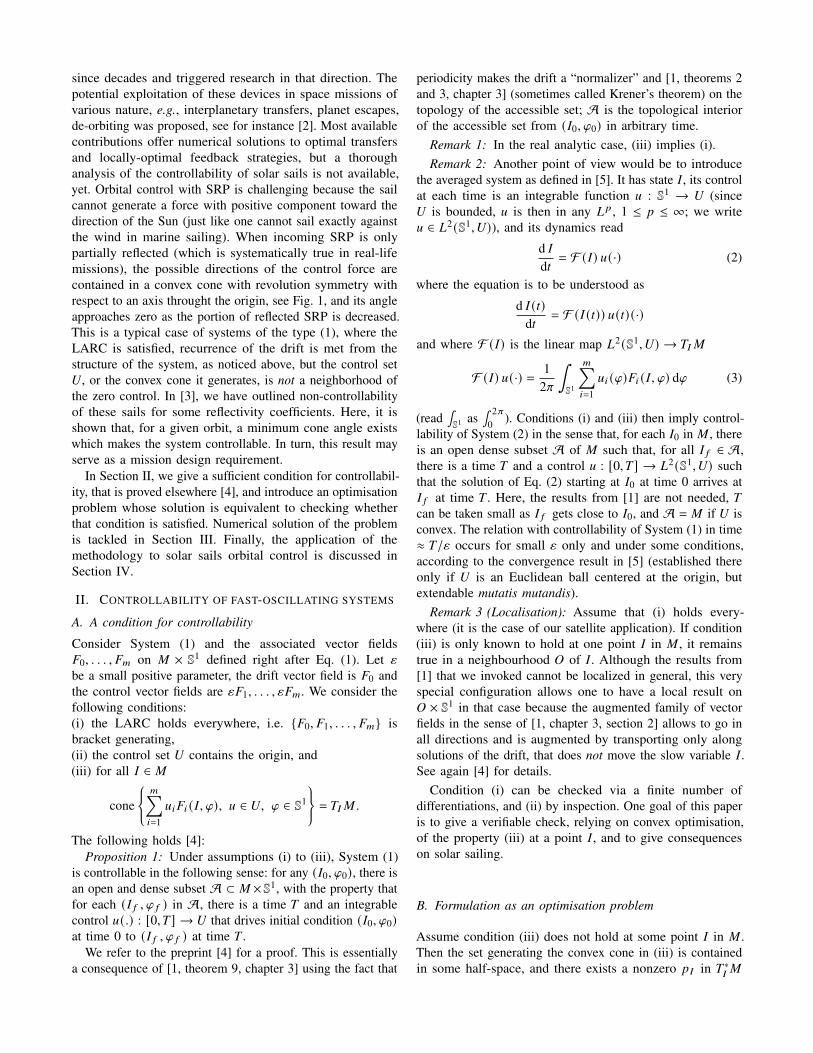
since decades and triggered research in that direction. Thepotential exploitation of these devices in space missions ofvarious nature, e.g., interplanetary transfers, planet escapes,de-orbiting was proposed, see for instance [2]. Most availablecontributions offer numerical solutions to optimal transfersand locally-optimal feedback strategies, but a thoroughanalysis of the controllability of solar sails is not available,yet. Orbital control with SRP is challenging because the sailcannot generate a force with positive component toward thedirection of the Sun (just like one cannot sail exactly againstthe wind in marine sailing). When incoming SRP is onlypartially reflected (which is systematically true in real-lifemissions), the possible directions of the control force arecontained in a convex cone with revolution symmetry withrespect to an axis throught the origin, see Fig. 1, and its angleapproaches zero as the portion of reflected SRP is decreased.This is a typical case of systems of the type (1), where theLARC is satisfied, recurrence of the drift is met from thestructure of the system, as noticed above, but the control set*, or the convex cone it generates, is not a neighborhood ofthe zero control. In [3], we have outlined non-controllabilityof these sails for some reflectivity coefficients. Here, it isshown that, for a given orbit, a minimum cone angle existswhich makes the system controllable. In turn, this result mayserve as a mission design requirement.

In Section II, we give a sufficient condition for controllabil-ity, that is proved elsewhere [4], and introduce an optimisationproblem whose solution is equivalent to checking whetherthat condition is satisfied. Numerical solution of the problemis tackled in Section III. Finally, the application of themethodology to solar sails orbital control is discussed inSection IV.

II. CONTROLLABILITY OF FAST-OSCILLATING SYSTEMS

A. A condition for controllability

Consider System (1) and the associated vector fields�0, . . . , �< on " × S1 defined right after Eq. (1). Let Ybe a small positive parameter, the drift vector field is �0 andthe control vector fields are Y�1, . . . , Y�<. We consider thefollowing conditions:(i) the LARC holds everywhere, i.e. {�0, �1, . . . , �<} isbracket generating,(ii) the control set * contains the origin, and(iii) for all � ∈ "

cone

{<∑8=1

D8�8 (�, i), D ∈ *, i ∈ S1

}= )�".

The following holds [4]:Proposition 1: Under assumptions (i) to (iii), System (1)

is controllable in the following sense: for any (�0, i0), there isan open and dense subset A ⊂ " ×S1, with the property thatfor each (� 5 , i 5 ) in A, there is a time ) and an integrablecontrol D(.) : [0, )] → * that drives initial condition (�0, i0)at time 0 to (� 5 , i 5 ) at time ) .

We refer to the preprint [4] for a proof. This is essentiallya consequence of [1, theorem 9, chapter 3] using the fact that

periodicity makes the drift a “normalizer” and [1, theorems 2and 3, chapter 3] (sometimes called Krener’s theorem) on thetopology of the accessible set; A is the topological interiorof the accessible set from (�0, i0) in arbitrary time.

Remark 1: In the real analytic case, (iii) implies (i).Remark 2: Another point of view would be to introduce

the averaged system as defined in [5]. It has state �, its controlat each time is an integrable function D : S1 → * (since* is bounded, D is then in any ! ?, 1 ≤ ? ≤ ∞; we writeD ∈ !2 (S1,*)), and its dynamics read

d �dC= F (�) D(·) (2)

where the equation is to be understood as

d � (C)dC

= F (� (C)) D(C) (·)

and where F (�) is the linear map !2 (S1,*) → )�"

F (�) D(·) = 12c

∫S1

<∑8=1

D8 (i)�8 (�, i) di (3)

(read∫S1 as

∫ 2c0 ). Conditions (i) and (iii) then imply control-

lability of System (2) in the sense that, for each �0 in " , thereis an open dense subset A of " such that, for all � 5 ∈ A,there is a time ) and a control D : [0, )] → !2 (S1,*) suchthat the solution of Eq. (2) starting at �0 at time 0 arrives at� 5 at time ) . Here, the results from [1] are not needed, )can be taken small as � 5 gets close to �0, and A = " if * isconvex. The relation with controllability of System (1) in time≈ )/Y occurs for small Y only and under some conditions,according to the convergence result in [5] (established thereonly if * is an Euclidean ball centered at the origin, butextendable mutatis mutandis).

Remark 3 (Localisation): Assume that (i) holds every-where (it is the case of our satellite application). If condition(iii) is only known to hold at one point � in ", it remainstrue in a neighbourhood $ of �. Although the results from[1] that we invoked cannot be localized in general, this veryspecial configuration allows one to have a local result on$ × S1 in that case because the augmented family of vectorfields in the sense of [1, chapter 3, section 2] allows to go inall directions and is augmented by transporting only alongsolutions of the drift, that does not move the slow variable �.See again [4] for details.

Condition (i) can be checked via a finite number ofdifferentiations, and (ii) by inspection. One goal of this paperis to give a verifiable check, relying on convex optimisation,of the property (iii) at a point �, and to give consequenceson solar sailing.

B. Formulation as an optimisation problem

Assume condition (iii) does not hold at some point � in " .Then the set generating the convex cone in (iii) is containedin some half-space, and there exists a nonzero ?� in )∗

�"

such that, for all D in * and all i in S1,⟨?� ,

<∑8=1

D8�8 (�, i)⟩≤ 0.

Actually this property even holds true for all D in

:= cone(*). (4)

This implies the weaker property that, for any squareintegrable control function D : S1 → ,

〈?� , F (�) D〉 ≤ 0 (5)

with F defined in Eq. (3). Let 40, . . . , 4= in )�" be thevertices of an =-simplex containing 0 in its interior. Thenegation of Eq. (5) is that, for all : = 0, . . . , =, there exists acontrol D in !2 (S1,R<) valued in such that

2c F (�) D = 4: .

This condition together with the cone constraint of Eq. (4)define feasibility conditions for the optimal control problemover )�" (remember that � is fixed) with quadratic cost∫

S1|D(i) |2 di→ min . (6)

This is indeed a control problem associated with the followingdynamics with state X� ∈ )�" and time i, where � appearsas a fixed parameter:

d X�di

=

<∑8=1

D8 �8 (�, i),

with control constraint D ∈ and boundary conditionsX� (0) = 0 and X� (2c) = 4: . Note that we have chosena quadratic cost in order to preserve the convexity of theproblem.

Remark 4: Given �: such that there is some curve in "

connecting �0 to �: with tangent vector 4: at �0, Problem (6)can serve as a proxy to find an admissible curve for theaveraged dynamics of System (2); this proxy being all themore accurate as �: is close to �0 in the manifold of slowvariables.

We show in the next section that this problem is accuratelyapproximated by a convex optimisation after approximating by a polyhedral cone and truncating the Fourier series ofthe control. Eventually, by proving feasibility of these controlproblems for every vertex 4: , one has an effective check oflocal controllability around � of the original problem.

III. DISCRETISATION OF THE SEMI-INFINITEOPTIMISATION PROBLEM

The discretisation of Problem (6) is achieved in two steps.First, is approximated by the polyhedral cone 6 ⊂

generated by �1, . . . , �6 chosen in m : admissible controlsare given by a conical combination of the form

D(i) =6∑9=1W 9 (i)� 9 , W 9 (i) ≥ 0, i ∈ S1, 9 = 1, . . . , 6.

Second, an #-dimensional basis of trigonometric polynomi-als, Φ(i) =

(1, 48i , 428i , . . . , 4 (#−1)8i ) , is used to model

functions W 9 as

W 9 (i) = (Φ(i) |2 9 )�where 2 9 ∈ C# are complex-valued vectors (serving asdesign variables of the finite-dimensional problem), and where(·|·)� is the Hermitian product on C# . Positivity constraintson the functions W 9 define a semi-infinite optimisationproblem; these constraints are enforced by leveraging on theformalism of squared functional systems outlined in [6] whichallows to recast continuous positivity constraints into linearmatrix inequalities (LMI). Specifically, given a trigonometricpolynomial ?(i) = (Φ(i) |2)� and the linear operatorΛ∗ : C#×# → C# associated to Φ(i) (more details areprovided in Appendix A), it holds

(∀i ∈ S1) : ?(i) ≥ 0⇐⇒ (∃ . � 0) : Λ∗ (. ) = 2.

For an admissible control D valued in 6, one has∫S1

<∑8=1

D8 (i)�8 (i) di =6∑9=1

(! 92 9 + !̄ 9 2̄ 9

)with ! 9 (�) in C=×# defined by

! 9 (�) =12

<∑8=1

∫S1�8 9�8 (�, i)Φ� (i) di,

where Φ� (i) denotes the Hermitian transpose and where� 9 = (�8 9 )8=1,...,<. We note that the components of ! 9 (�)are Fourier coefficients of the function

∑<8=1 �8 9�8 (�, i). The

discrete Fourier transform (DFT) can be used to approximate! 9 (�). Since vector fields �8 are smooth, truncation of theseries is justified by the fast decrease of the coefficients.Finally, for a control D valued in 6 with coefficients W 9that are truncated Fourier series of order # − 1, the !2 normover S1 is easily expressed in terms the coefficients 2 9 usingorthogonality of the family of complex exponentials:

12

∫S1|D(i) |2 di =

12

6∑9 ,;=1

#−1∑:=0

�); � 9

(2̄;:2 9: + 2;: 2̄ 9:

)=

6∑;, 9=1

�); � 9 (2 9 |2;)� .

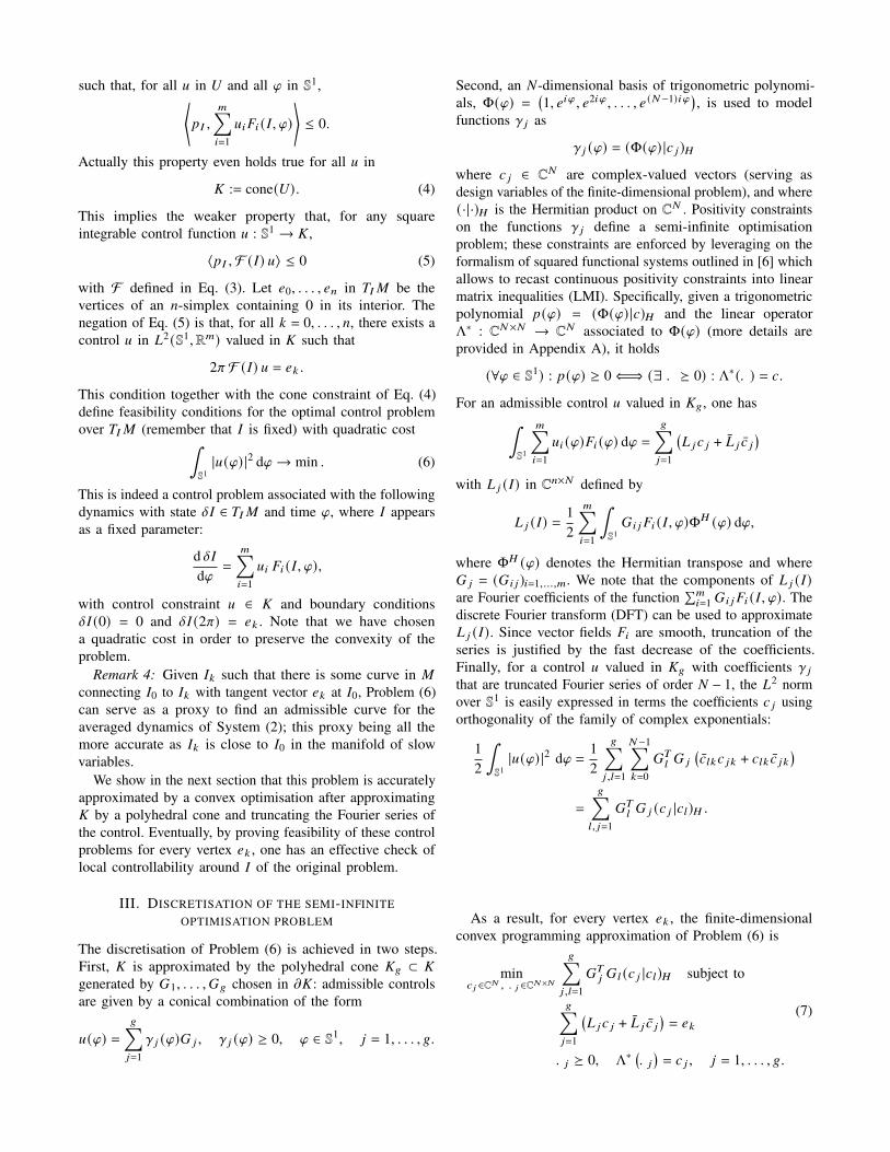
As a result, for every vertex 4: , the finite-dimensionalconvex programming approximation of Problem (6) is

min2 9 ∈C# , .9 ∈C#×#

6∑9 ,;=1

�)9 �; (2 9 |2;)� subject to

6∑9=1

(! 92 9 + !̄ 9 2̄ 9

)= 4:

. 9 � 0, Λ∗(. 9

)= 2 9 , 9 = 1, . . . , 6.

(7)

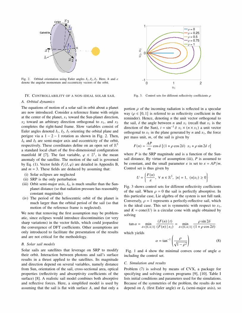
Fig. 2. Orbital orientation using Euler angles �1, �2, �3. Here, ℎ and 4denote the angular momentum and eccentricity vectors of the orbit.

IV. CONTROLLABILITY OF A NON-IDEAL SOLAR SAIL

A. Orbital dynamics

The equations of motion of a solar sail in orbit about a planetare now introduced. Consider a reference frame with originat the center of the planet, G1 toward the Sun-planet direction,G2 toward an arbitrary direction orthogonal to G1, and G3completes the right-hand frame. Slow variables consist ofEuler angles denoted �1, �2, �3 orienting the orbital plane andperigee via a 1 − 2 − 1 rotation as shown in Fig. 2. Then,�4 and �5 are semi-major axis and eccentricity of the orbit,respectively. These coordinates define on an open set of R5

a standard local chart of the five-dimensional configurationmanifold " [7]. The fast variable, i ∈ S1, is the meananomaly of the satellite. The motion of the sail is governedby Eq. (1). Vector fields �8 (�, i) are detailed in Appendix B,and < = 3. These fields are deduced by assuming that:

(i) Solar eclipses are neglected(ii) SRP is the only perturbation

(iii) Orbit semi-major axis, �4, is much smaller than the Sun-planet distance (so that radiation pressure has reasonablyconstant magnitude)

(iv) The period of the heliocentric orbit of the planet ismuch larger than the orbital period of the sail (so thatmotion of the reference frame is neglected).

We note that removing the first assumption may be problem-atic, since eclipses would introduce discontinuities (or verysharp variations) in the vector fields, which could jeopardisethe convergence of DFT coefficients. Other assumptions areonly introduced to facilitate the presentation of the resultsand are not critical for the methodology.

B. Solar sail models

Solar sails are satellites that leverage on SRP to modifytheir orbit. Interaction between photons and sail’s surfaceresults in a thrust applied to the satellites. Its magnitudeand direction depend on several variables, namely distancefrom Sun, orientation of the sail, cross-sectional area, opticalproperties (reflectivity and absorptivity coefficients of thesurface) [8]. A realistic sail model combines both absorptiveand reflective forces. Here, a simplified model is used byassuming that the sail is flat with surface �, and that only a

0 1 2-1

0

1 = 0

= 0.25

= 0.5

= 0.75

= 1

Fig. 3. Control sets for different reflectivity coefficients d

portion d of the incoming radiation is reflected in a specularway (d ∈ [0, 1] is referred to as reflectivity coefficient in thereminder). Hence, denoting = the unit vector orthogonal tothe sail, X the angle between = and G1 (recall that G1 is thedirection of the Sun), C = sin−1 X G1 × (= × G1) a unit vectororthogonal to G1 in the plane generated by = and G1, the forceper mass unit, <, of the sail is given by

� (=) = �%

<cos X [(1 + d cos 2X) G1 + d sin 2X C]

where % is the SRP magnitude and is a function of the Sun-sail distance. By virtue of assumption (iii), % is assumed tobe constant, and the small parameter Y is set to Y = �%/<.Control set is thus given by

* =

{� (=)Y

, ∀ = ∈ R3, |=| = 1, (=|G1) ≥ 0}

Fig. 3 shows control sets for different reflectivity coefficientsof the sail. When d = 0 the sail is perfectly absorptive. Inthis particular case, Lie algebra of the system is not full rank.Conversely, d = 1 represents a perfectly-reflective sail, whichis the ideal case. This set is symmetric with respect to G1,and = cone(*) is a circular cone with angle obtained bysolving

tanU = minX∈[0, c/2]

(� (=) | C)(� (=) | G1)

= minX∈[0, c/2]

d sin 2X(1 + d cos 2X)

which yields

U = tan−1

(d√

1 − d2

)(8)

Fig. 1 and 4 show the minimal convex cone of angle Uincluding the control set.

C. Simulation and results

Problem (7) is solved by means of CVX, a package forspecifying and solving convex programs [9], [10]. Table Ilists initial conditions and parameters used for the simulations.Because of the symmetries of the problem, the results do notdepend on �1 (first Euler angle) or �4 (semi-major axis), so

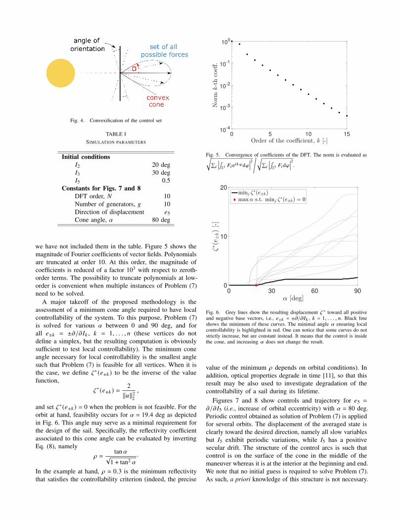
Fig. 4. Convexification of the control set

TABLE ISIMULATION PARAMETERS

Initial conditions�2 20 deg�3 30 deg�5 0.5

Constants for Figs. 7 and 8DFT order, # 10Number of generators, 6 10Direction of displacement 45Cone angle, U 80 deg

we have not included them in the table. Figure 5 shows themagnitude of Fourier coefficients of vector fields. Polynomialsare truncated at order 10. At this order, the magnitude ofcoefficients is reduced of a factor 103 with respect to zeroth-order terms. The possibility to truncate polynomials at low-order is convenient when multiple instances of Problem (7)need to be solved.

A major takeoff of the proposed methodology is theassessment of a minimum cone angle required to have localcontrollability of the system. To this purpose, Problem (7)is solved for various U between 0 and 90 deg, and forall 4±: = ±m/m�: , : = 1, . . . , = (these vertices do notdefine a simplex, but the resulting computation is obviouslysufficient to test local controllability). The minimum coneangle necessary for local controllability is the smallest anglesuch that Problem (7) is feasible for all vertices. When it isthe case, we define Z∗ (4±: ) to be the inverse of the valuefunction,

Z∗ (4±: ) =2‖D‖22

,

and set Z∗ (4±: ) = 0 when the problem is not feasible. For theorbit at hand, feasibility occurs for U = 19.4 deg as depictedin Fig. 6. This angle may serve as a minimal requirement forthe design of the sail. Specifically, the reflectivity coefficientassociated to this cone angle can be evaluated by invertingEq. (8), namely

d =tanU

√1 + tan2 U

·

In the example at hand, d ' 0.3 is the minimum reflectivitythat satisfies the controllability criterion (indeed, the precise

0 5 10 1510

-4

10-3

10-2

10-1

100

Fig. 5. Convergence of coefficients of the DFT. The norm is evaluated as√∑8

���∫S1 �8e8:idi���2/√∑

8

���∫S1 �8di���2.

0 30 60 900

10

20

Fig. 6. Grey lines show the resulting displacement Z ∗ toward all positiveand negative base vectors, i.e., 4±: = ±m/m�: , : = 1, . . . , =. Black lineshows the minimum of these curves. The minimal angle U ensuring localcontrollability is highlighted in red. One can notice that some curves do notstrictly increase, but are constant instead. It means that the control is insidethe cone, and increasing U does not change the result.

value of the minimum d depends on orbital conditions). Inaddition, optical properties degrade in time [11], so that thisresult may be also used to investigate degradation of thecontrollability of a sail during its lifetime.

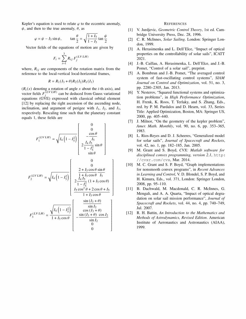
Figures 7 and 8 show controls and trajectory for 45 =m/m�5 (i.e., increase of orbital eccentricity) with U = 80 deg.Periodic control obtained as solution of Problem (7) is appliedfor several orbits. The displacement of the averaged state isclearly toward the desired direction, namely all slow variablesbut �5 exhibit periodic variations, while �5 has a positivesecular drift. The structure of the control arcs is such thatcontrol is on the surface of the cone in the middle of themaneuver whereas it is at the interior at the beginning and end.We note that no initial guess is required to solve Problem (7).As such, a priori knowledge of this structure is not necessary.

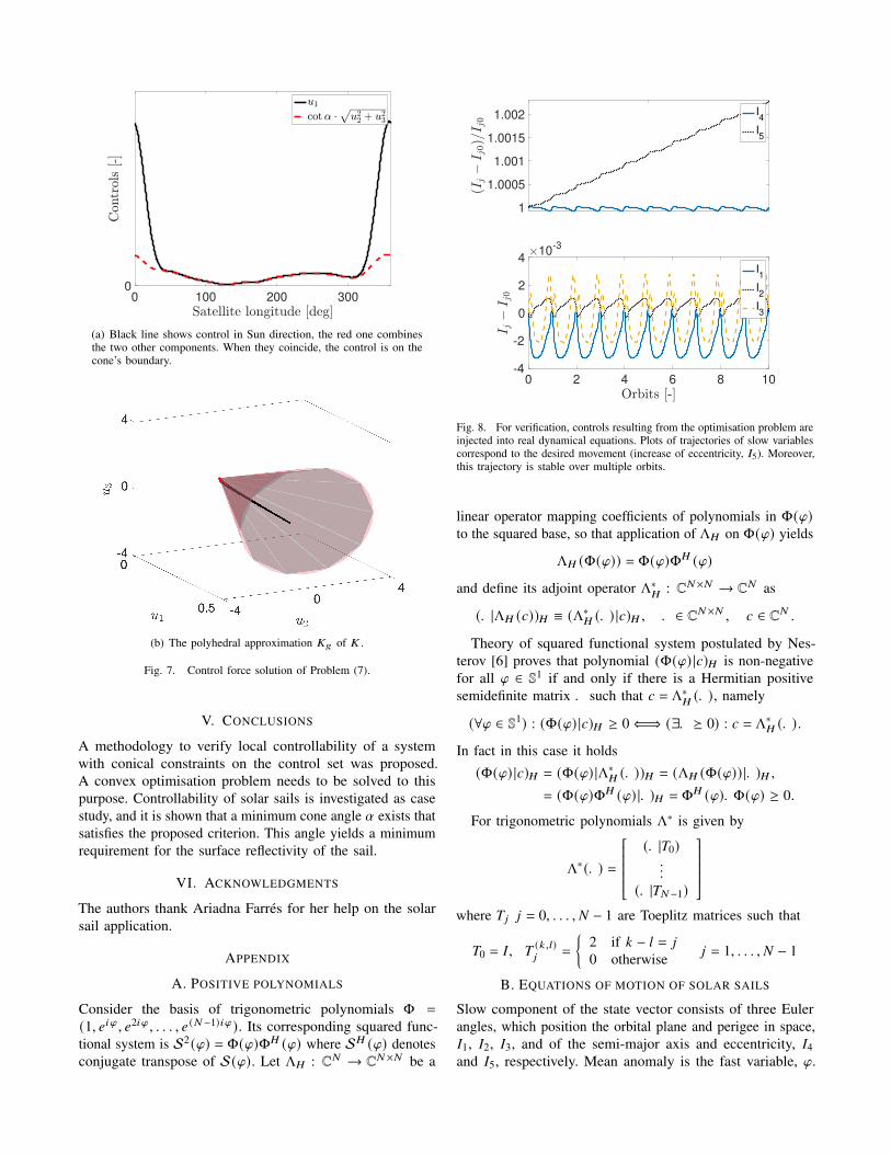
0 100 200 3000

(a) Black line shows control in Sun direction, the red one combinesthe two other components. When they coincide, the control is on thecone’s boundary.

(b) The polyhedral approximation 6 of .

Fig. 7. Control force solution of Problem (7).

V. CONCLUSIONS

A methodology to verify local controllability of a systemwith conical constraints on the control set was proposed.A convex optimisation problem needs to be solved to thispurpose. Controllability of solar sails is investigated as casestudy, and it is shown that a minimum cone angle U exists thatsatisfies the proposed criterion. This angle yields a minimumrequirement for the surface reflectivity of the sail.

VI. ACKNOWLEDGMENTS

The authors thank Ariadna Farrés for her help on the solarsail application.

APPENDIX

A. POSITIVE POLYNOMIALS

Consider the basis of trigonometric polynomials Φ =

(1, 48i , 428i , . . . , 4 (#−1)8i). Its corresponding squared func-tional system is S2 (i) = Φ(i)Φ� (i) where S� (i) denotesconjugate transpose of S(i). Let Λ� : C# → C#×# be a

1

1.0005

1.001

1.0015

1.002 I4

I5

0 2 4 6 8 10-4

-2

0

2

410

-3

I1

I2

I3

Fig. 8. For verification, controls resulting from the optimisation problem areinjected into real dynamical equations. Plots of trajectories of slow variablescorrespond to the desired movement (increase of eccentricity, �5). Moreover,this trajectory is stable over multiple orbits.

linear operator mapping coefficients of polynomials in Φ(i)to the squared base, so that application of Λ� on Φ(i) yields

Λ� (Φ(i)) = Φ(i)Φ� (i)

and define its adjoint operator Λ∗�

: C#×# → C# as

(. |Λ� (2))� ≡ (Λ∗� (. ) |2)� , . ∈ C#×# , 2 ∈ C# .

Theory of squared functional system postulated by Nes-terov [6] proves that polynomial (Φ(i) |2)� is non-negativefor all i ∈ S1 if and only if there is a Hermitian positivesemidefinite matrix . such that 2 = Λ∗

�(. ), namely

(∀i ∈ S1) : (Φ(i) |2)� ≥ 0⇐⇒ (∃. � 0) : 2 = Λ∗� (. ).

In fact in this case it holds

(Φ(i) |2)� = (Φ(i) |Λ∗� (. ))� = (Λ� (Φ(i)) |. )� ,= (Φ(i)Φ� (i) |. )� = Φ� (i).Φ(i) ≥ 0.

For trigonometric polynomials Λ∗ is given by

Λ∗ (. ) =(. |)0)...

(. |)#−1)

where )9 9 = 0, . . . , # − 1 are Toeplitz matrices such that

)0 = �, )(:,;)9

=

{2 if : − ; = 90 otherwise 9 = 1, . . . , # − 1

B. EQUATIONS OF MOTION OF SOLAR SAILS

Slow component of the state vector consists of three Eulerangles, which position the orbital plane and perigee in space,�1, �2, �3, and of the semi-major axis and eccentricity, �4and �5, respectively. Mean anomaly is the fast variable, i.

Kepler’s equation is used to relate i to the eccentric anomaly,k, and then to the true anomaly, \, as

i = k − �5 sink, tan\

2=

√1 + �51 − �5

tank

2Vector fields of the equations of motion are given by

�8 =

3∑8=1

'8 9 �(!+ !� )9

where, '8 9 are components of the rotation matrix from thereference to the local-vertical local-horizontal frames,

' = '1 (�3 + \)'2 (�2)'1 (�1)

('8 (G) denoting a rotation of angle G about the 8-th axis), andvector fields � (!+ !� )

9can be deduced from Gauss variational

equations (GVE) expressed with classical orbital element[12] by replacing the right ascension of the ascending node,inclination, and argument of perigee with �1, �2, and �3,respectively. Rescaling time such that the planetary constantequals 1, these fields are

�(!+ !� )1 =

√�4

(1 − �2

5

)

00

−cos \�5

2�4 �5

1 − �25

sin \

sin \

�(!+ !� )2 =

√�4

(1 − �2

5

)

00

2 + �5 cos \1 + �5 cos \

sin \�5

2�4 �5

1 − �25(1 + �5 cos \)

�5 cos2 \ + 2 cos \ + �51 + �5 cos \

�(!+ !� )3 =

√�4

(1 − �2

5

)1 + �5 cos \

sin (�3 + \)sin �2

cos (�3 + \)− sin (�3 + \) cos �2

sin �200

REFERENCES

[1] V. Jurdjevic, Geometric Control Theory, 1st ed. Cam-bridge University Press, Dec. 28, 1996.

[2] C. R. McInnes, Solar Sailing. London: Springer Lon-don, 1999.

[3] A. Herasimenka and L. Dell’Elce, “Impact of opticalproperties on the controllability of solar sails”, ICATT2021.

[4] J.-B. Caillau, A. Herasimenka, L. Dell’Elce, and J.-B.Pomet, “Control of a solar sail”, preprint.

[5] A. Bombrun and J.-B. Pomet, “The averaged controlsystem of fast-oscillating control systems”, SIAMJournal on Control and Optimization, vol. 51, no. 3,pp. 2280–2305, Jan. 2013.

[6] Y. Nesterov, “Squared functional systems and optimiza-tion problems”, in High Performance Optimization,H. Frenk, K. Roos, T. Terlaky, and S. Zhang, Eds.,red. by P. M. Pardalos and D. Hearn, vol. 33, SeriesTitle: Applied Optimization, Boston, MA: Springer US,2000, pp. 405–440.

[7] J. Milnor, “On the geometry of the kepler problem”,Amer. Math. Monthly, vol. 90, no. 6, pp. 353–365,1983.

[8] L. Rios-Reyes and D. J. Scheeres, “Generalized modelfor solar sails”, Journal of Spacecraft and Rockets,vol. 42, no. 1, pp. 182–185, Jan. 2005.

[9] M. Grant and S. Boyd, CVX: Matlab software fordisciplined convex programming, version 2.1, http://cvxr.com/cvx, Mar. 2014.

[10] M. C. Grant and S. P. Boyd, “Graph implementationsfor nonsmooth convex programs”, in Recent Advancesin Learning and Control, V. D. Blondel, S. P. Boyd, andH. Kimura, Eds., vol. 371, London: Springer London,2008, pp. 95–110.

[11] B. Dachwald, M. Macdonald, C. R. McInnes, G.Mengali, and A. A. Quarta, “Impact of optical degra-dation on solar sail mission performance”, Journal ofSpacecraft and Rockets, vol. 44, no. 4, pp. 740–749,Jul. 2007.

[12] R. H. Battin, An Introduction to the Mathematics andMethods of Astrodynamics, Revised Edition. AmericanInstitute of Aeronautics and Astronautics (AIAA),1999.