Effective ﬁeld theory for halo nuclei: shallow p-wave …faculty.tamuc.edu/cbertulani/cab/papers/NPA_712_37.pdfEffective ﬁeld theory for halo nuclei: shallow p-wave states C.A

Nuclear Physics A 712 (2002) 37–58

www.elsevier.com/locate/npe

Effective field theory for halo nuclei:shallowp-wave states

C.A. Bertulania, H.-W. Hammerb, U. van Kolckc,d

a National Superconducting Cyclotron Laboratory, Michigan State University, East Lansing, MI 48824, USAb Department of Physics, The Ohio State University, Columbus, OH 43210, USA

c Department of Physics, University of Arizona, Tucson, AZ 85721, USAd RIKEN-BNL Research Center, Brookhaven National Laboratory, Upton, NY 11973, USA

Received 24 May 2002; received in revised form 12 August 2002; accepted 5 September 2002

Abstract

Halo nuclei are a promising new arena for studies based on effective field theory (EFT). Wedevelop an EFT for shallowp-wave states and discuss the application to elasticnα scattering. Incontrast to thes-wave case, both the scattering length and effective range enter at leading order. Wealso discuss the prospects of using EFT in the description of other halos, such as the three-body halonucleus6He. 2002 Elsevier Science B.V. All rights reserved.

PACS: 21.45.+v; 25.40.Dn

Keywords: Effective field theory; Shallowp-wave states; Halo nuclei

1. Introduction

Nuclear halo states have been found in a number of light nuclei close to the nucleondrip lines. They are characterized by a very low separation energy of the valence nucleon(or cluster of nucleons). As a consequence, the nuclear radius is very large compared to thesize of the tightly bound core. The large size of halo nuclei leads to threshold phenomenawith important general consequences for low-energy reaction rates in nuclear astrophysics.One example is the reactionp + 7Be→ 8B + γ which is important for solar neutrinoproduction. The nucleus8B is believed to be a two-body proton halo, consisting of a7Becore and a proton [1]. Somewhat more complicated are three-body halos consisting of a

E-mail address: [email protected] (H.-W. Hammer).

0375-9474/02/$ – see front matter 2002 Elsevier Science B.V. All rights reserved.PII: S0375-9474(02)01270-8

38 C.A. Bertulani et al. / Nuclear Physics A 712 (2002) 37–58

core and two slightly bound nucleons. Particularly interesting are Borromean three-bodyhalos, where no two-body subsystem is bound. Typical examples are6He and11Li, whichconsist of a4He and9Li core, respectively, and two neutrons. For reviews of halo nuclei,see Ref. [2]. The physics of halo nuclei is an important part of the physics program at RIA[3]. A thorough discussion of reactions with rare isotopes can be found in Ref. [4].

The physics of halo nuclei is a promising new arena for effective field theory (EFT).EFTs provide a powerful framework to explore separation of scales in physical systemsin order to perform systematic, model-independent calculations [5]. If, for example, therelative momentumk of two particles is much smaller than the inverse range of theirinteraction 1/R, observables can be expanded in powers ofkR. All short-distance effectsare systematically absorbed into a few low-energy constants using renormalization. TheEFT approach allows for systematically improvable calculations of low-energy processeswith well-defined error estimates. The long-distance physics is included explicitly, whilethe corrections from short-distance physics are calculated in an expansion in the ratio ofthese two scales.1 The inherent separation of length scales in halo nuclei makes them anideal playing ground for EFT.

In recent years, there has been much interest in applying EFT methods to nuclearsystems [6,7]. Up to now, nuclear EFT has mainly been applied to two-, three-, and four-nucleon systems starting from a fundamental nucleon–nucleon interaction. The originalmotivation was to understand the gross features of nuclear systems from a QCD perspectiveby deriving the nuclear potential and currents relevant for momenta comparable to the pionmass (p ∼ mπ ) [8]. More recently, it has been realized that it is possible to carry outvery precise calculations for fundamental physics processes at lower energies. For verylow momenta (p mπ ), even pion exchange can be considered “short-distance” physics.In this case, one can use an effective Lagrangian including only contact interactions. Thelarge s-wave scattering lengths require that the leading two-body contact interaction betreated non-perturbatively [9,10]. In the two-nucleon system, this program has been verysuccessful (see, e.g., Refs. [6,11] and references therein).

Using EFT, one can relate low-energy measurements in one reaction to observablesin a similar (but unmeasured) reaction in a controlled expansion with reliable errorestimates. This is in contrast to standard potential model calculations where errors canonly be estimated by comparing different potentials. An example of a precise calculationin the “pionless” EFT is the reactionn + p → d + γ [12], which is relevant to big-bang nucleosynthesis (BBN). As for many other reactions of astrophysical interest, theuncertainty in the cross section is difficult to determine due to the lack of data at lowenergies and the lack of information about theoretical estimates. In the energy of relevanceto BBN, both E1 and M1 capture are important. They have been calculated to fifth and thirdorder, respectively, where two new counterterms appear. Using the measured cold-capturerate and data for the deuteron photodisintegration reaction to fix the counterterms, then+p→ d+γ cross section was computed to 1% for center-of-mass energiesE 1 MeV.

1 Note that “effective theory” is sometimes used in reference to a model that captures the essence of therelevant long-distance physics without necessarily accounting for the short-distance physics in a systematic way.Here we use “EFT” in the model-independent sense described above, in which “power counting” of the differentorders in the expansion is a crucial ingredient.

C.A. Bertulani et al. / Nuclear Physics A 712 (2002) 37–58 39

Much of the strength of EFT lies in the fact that it can be applied without off-shellambiguities to systems with more nucleons. The crucial issue of the relative size ofthree-body forces has been investigated in the three-body system [13]. Nucleon–deuteronscattering in all channels except thes1/2-wave can be calculated to high orders usingtwo-nucleon input only, with results in striking agreement with data and potential-modelcalculations [14]. For example, to third order, thes3/2 scattering length is found to be

a(EFT)3/2 = 6.33± 0.10 fm, to be compared to the measureda

(expt)3/2 = 6.35± 0.02 fm. In

contrast, in thes1/2-wave channel, the non-perturbative running of the renormalizationgroup requires a momentum-independent three-body force in leading order [15]. Once thenew parameter is fitted to (say) the scattering length, the energy dependence is predicted.The triton binding energy, for example, is found to beB

(EFT)3 = 8.0 MeV in leading order,

already pretty close to the experimentalB(expt)3 = 8.5 MeV. Recently, this approach was

also applied toΛd scattering and the hypertriton [16]. Using the hypertriton binding energyto fix the three-body force, the low-energyΛd scattering observables can be predicted. Theresults are very insensitive to the poorly knownΛN low-energy parameters. In a relatedstudy, theΛd Phillips line was established [17].

However, in an EFT it is, by no means, necessary to start from a fundamental nucleon–nucleon interaction. If, as in halo nuclei, the core is much more tightly bound than theremaining nucleons, it can be treated as an explicit degree of freedom. One can write anEFT for the contact interactions of the nucleons with the core and include the substructureof the core perturbatively in a controlled expansion. This approach is appropriate forenergies smaller than the excitation energy of the core. In other words, one can accountfor the spatial extension of the core by treating it as a point particle with corrections fromits finite size entering in a derivative expansion of the interaction. This is a consequenceof the limited resolution of a long wavelength probe which cannot distinguish between apoint and an extended particle of sizeR if the wavelengthλR.

In this paper, we consider the virtualp-wave state innα scattering as a test case. Eventhough there is no bound state in this channel, it has all the characteristics of a two-bodyhalo nucleus. Furthermore it is relevant for the study of the Borromean three-body halo6He, which will be addressed in a forthcoming publication [18]. Elasticnα scattering isrelatively well-known experimentally. Since the nucleon hasj = 1/2 and theα particlehasj = 0, there are contributions from ans-wave (s1/2), two p-waves (p1/2 andp3/2),etc. Arndt et al. performed a phase-shift analysis of low-energy data and extracted theeffective-range parameters in thes- andp-waves [19]. Thep3/2 partial wave displays aresonance atE ∼ 1 MeV corresponding to a shallow virtual bound state, while thes1/2andp1/2 partial waves are non-resonant at low energies. We will show that thisp-waveresonance leads to a power counting different from the one fors-wave bound states [9,10]that has been discussed extensively in the literature because of its relevance for the no-coreEFT.2 In particular, proper renormalization requires two low-energy parameters at leadingorder, namely the scattering length and the effective range. The extension to higher ordersis straightforward. As we will see, the EFT describes the low-energy data very well.

2 By no-core EFT we mean an EFT where all nuclei are dynamically generated from nucleon (and possiblypion and delta isobar) degrees of freedom.


The organization of this paper is as follows: in Section 2, we work out renormalizationand power counting for ap-wave resonance in the simpler context of spinless fermions.In Section 3, we include the spin and isospin of the nucleon and apply our formalismto elasticnα scattering. In Section 4, we summarize our results and present an outlook. Inparticular, we discuss the extension to the Borromean three-body halo6He and the reactionp+ 7Be→ 8B+ γ .

2. EFT for shallow p-wave states

In this section, we develop the power counting for shallowp-wave states (bound statesor virtual states) in the particularly simple case of a hypothetical system of two spinlessfermions of common massm. Our arguments are a generalization of those in Ref. [9].

In order to have a shallow bound state, we need at least two momentum scales: thebreakdown scale of the EFT,Mhi, and a second scale,Mlo Mhi, that characterizesthe shallow bound state. The scaleMhi is set by the degrees of freedom that have beenintegrated out. In the case of an EFT without explicit pions and core excitations,Mhi isthe smallest between the pion massmπ and the momentum corresponding to the energy ofthe first excited state. The scaleMlo is not a fundamental scale of the underlying theory. Itcan be understood as arising from a fine-tuning of the parameters in the underlying theory.If the values of these parameters were changed slightly, the scaleMlo would disappear.We seek an ordering of contributions at the scaleMlo in powers ofMlo/Mhi. Due to thepresence of fine-tuning, naive dimensional analysis cannot be applied.

For simplicity we neglect relativistic corrections. They are generically small becausethey are suppressed by powers of the particle massm, and in the cases of interest heremMhi. They can be included along the lines detailed in Ref. [9].

2.1. Natural case

First, we will consider the natural case without any fine-tuning. The scale of all low-energy parameters is then set byMhi and naive dimensional analysis can be applied.

TheT -matrix for the non-relativistic scattering of two spinless fermions with massm

in the center-of-mass frame can be expanded in partial waves as

T (k,cosθ)=∑l0

Tl(k,cosθ)= 4π

m

∑l0

2l + 1

k cotδl − ikPl(cosθ), (1)

where k is the center-of-mass momentum,θ the scattering angle, andPl(cosθ) is aLegendre polynomial.3 The generalized effective-range expansion for arbitrary angularmomentuml reads:

k2l+1 cotδl =− 1

al+ rl

2k2− Pl

4k4+ · · · , (2)

3 Note that we assume the two fermions are distinguishable.


whereal , rl , andPl are the scattering length, effective range, and shape parameter in thelth partial wave, respectively. Forl = 0, Eq. (2) reproduces the familiar effective-rangeexpansion fors-waves. Note that the dimension of the effective-range parameters dependson the partial wave. In thes-wave,a0 and r0 have dimensions of length, whileP0 hasdimensions of (length)3. For p-waves,a1 has dimension of (length)3 (it is a scattering“volume”), r1 has dimension 1/(length) (it is an “effective momentum”), andP1 hasdimension of length.

Thes-wave contributionT0 has been discussed in detail in the literature [9,10]. Our goalhere is to set up an EFT that reproduces thep-wave contributionT1 in a low-momentumexpansion,

T1(k,cosθ) = −12πa1

mk2 cosθ

(1+ a1r1

2k2− ia1k

3+ a1

4

(a1r

21 −P1

)k4+ · · ·

).

(3)

We start with the most general Lagrangian for spinless fermions withp-waveinteractions:

L = ψ†[i∂0+

−→∇ 2

2m

]ψ + C

p

2

8

(ψ↔∇i ψ

)†(ψ↔∇ i ψ

)

− Cp4

64

[(ψ↔∇ 2 ↔∇ i ψ

)†(ψ↔∇ i ψ

)+H.c.]+ · · · , (4)

where↔∇= ←−∇ − −→∇ is the Galilean invariant derivative, H.c. denotes the Hermitian

conjugate, and the dots denote higher-derivative interactions that are suppressed at lowenergies. The fermion propagator is simply

iS(p0,p)= i

p0− p2/2m+ iε, (5)

and the Feynman rules for the vertices can be read off Eq. (4). Around the non-relativisticlimit, all interaction coefficients contain a common factor of 1/m that follows fromGalilean invariance. From dimensional analysis, we haveC

p

2 ∼ 12π/mM3hi and C

p

4 ∼12π/mM5

hi. The exact relation ofCp

2 andCp

4 to the scattering length and effective rangewill be obtained in the end from matching to Eq. (3).

We work in the center-of-mass frame and assign the momenta±k and±k′ to theincoming and outgoing particles, respectively. The total energy isE = k2/m = k′2/m.The EFT expansion is in powers ofk/Mhi. The leading contribution toT1 is of order12πk2/mM3

hi. It is given by the tree-level diagram with theCp

2 interaction shown inFig. 1(a). The result is simply

iT1(a) =−iCp

2 k · k′. (6)

The second term in the low-momentum expansion is suppressed byk2/M2hi compared to

the leading order. It is given by the tree-level diagram with theCp4 interaction shown in

Fig. 1(b):

iT1(b) =−iCp

4 k2 k · k′. (7)


Fig. 1. Lowest-order diagrams for the perturbative expansion ofT1. Particle propagators are represented by solidlines. TheCp

2 (Cp4 ) vertex is indicated by the open circle (crossed circle).

At order 12πk5/mM6hi, we have the one-loop diagram with twoCp

2 interactions shown inFig. 1(c). The contribution of this diagram is

iT1(c) =(−iCp

2

)2∫ d4q

(2π)4

iq · kE2 + q0− q2

2m + iε

iq · k′E2 − q0− q2

2m + iε

= (C

p

2

)2imk′ikj

∫d3q

(2π)3

qiqj

q2− k2− iε, (8)

where thedq0 integral was performed via contour integration. The remaining integral mustbe proportional toδij since no other vectors are available. Adding and subtractingk2 in thenumerator, we find

iT1(c) =(C

p2

)2 im

6π2 k · k′∫

dq q2+ k2∫

dq + k4∫

dq1

q2− k2− iε

= (C

p

2

)2 im

6π2k · k′

L3+ k2L1+ π

2ik3, (9)

whereL3 and L1 are infinite constants. These two ultraviolet divergent terms can beabsorbed by redefining the low-energy constantsC

p

2 and Cp

4 , respectively, which arealready present inT1(a) and T1(b). No new parameter enters at this order. The seriesproceeds in an obvious way.

We can now match to Eq. (3) to relate the renormalized coefficients to the effective-range parameters. We find from Eq. (6) thatC

p

2 = 12πa1/m, and from Eq. (7) thatCp

4 =C

p

2 r1a1/2. After renormalization,T1(c) reproduces the third term in the low-momentumexpansion of Eq. (3). Note that diagram 1(c) cannot be renormalized byC

p

2 alone eventhough it does not contain aCp

4 vertex. This observation has important consequences inthe unnatural case with fine-tuning.

2.2. Unnatural case

Now we turn to the more interesting case with a shallowp-wave state. In Refs. [9,10],it was shown that for a shallows-wave state the leading-order contact interactionC0 hasto be treated non-perturbatively. In this case,C0 is enhanced by a factorMhi/Mlo over theexpectationC0 ∼ 4π/mMhi from naive dimensional analysis. Adding a new rung in theladder forming the amplitude means adding an intermediate state (∼ mk/4π ) and aC0(∼ 4π/mMlo). Since the physics of the bound state is determined byk ∼Mlo, C0 has tobe summed to all orders.


For p-waves matters are slightly more complicated. We have seen above that therenormalization of the one-loop diagram with twoCp

2 interactions requires tree-levelcounterterms corresponding to both the leadingC

p

2 and subleadingCp

4 interaction. Asconsequence, at least theCp

2 andCp4 interactions have to be treated non-perturbatively if a

shallowp-wave state is present.Bound (virtual) states are associated with poles in theS-matrix on the upper (lower)

half of the complex momentum plane. The characteristic momentumγ of the bound/virtualstate is given by position of the pole,|k| ≡ γ . For a shallowp-wave state withγ ∼Mlo,the magnitude of both the effective range and the scattering length must be set byMlo. Thisis a consequence of the renormalization argument from the previous subsection. EitherC

p

2andCp

4 are both enhanced or they are both natural. Assuming that the higher terms in theeffective-range expansion are natural, the order of magnitude of the first three terms in theexpansion is

k3 cotδ1∼M3lo +Mlok

2+ 1

Mhik4+ · · · , (10)

and the effective-range parameters scale as

1

a1∼M3

lo,r1

2∼Mlo and

P1

4∼ 1

Mhi. (11)

Both Cp

2 andCp

4 are enhanced over the expectation from naive dimensional analysis andscale as

Cp

2 ∼12π

mM3lo

and Cp

4 ∼12π

mM5lo

. (12)

Consequently, for momenta of orderMlo neither interaction can be treated perturbatively.The shape parameterP1, however, is of order 1/Mhi and its contribution is suppressed byMlo/Mhi compared to the leading order.

In the following, we will demonstrate that treating theCp

2 and Cp

4 interactions toall orders is indeed sufficient for proper renormalization and, moreover, required toreproduce the physics of the shallowp-wave state. We will also work out the leading-orderdescription of a shallowp-wave state.

For convenience, we will not use the Lagrangian (4) but follow Ref. [20] and introducean auxiliary field (the dimeron) for the two-particle state. The corresponding Lagrangianis,

L = ψ†[i∂0+

−→∇ 2

2m

]ψ + η1d

†i

(i∂0+

−→∇ 2

4m−∆1

)di

+ g1

4

(d

†i

(ψ↔∇ i ψ

)+H.c.)+ · · · , (13)

where the signη1 =±1 and the parametersg1 and∆1 will be fixed from matching. ThisLagrangian contains exactly the same number of parameters as the original Lagrangian (4).Up to higher-order terms, Eq. (13) is equivalent to Eq. (4), as can be seen by performingthe Gaussian path integral overdi .


Fig. 2. The full dimeron propagator (thick shaded line) is obtained by dressing the bare dimeron propagator(double solid line) with particle bubbles (solid lines) to all orders.

The bare dimeron propagator is given by

iD01(p0,p)ij = iη1δij

p0− p2/4m−∆1+ iε. (14)

Summing theCp2 andC

p4 interactions to all orders in the theory without the dimeron

corresponds to dressing the bare dimeron propagator with particle bubbles to all orders.This summation is shown diagrammatically in Fig. 2. The full dimeron propagator is mosteasily calculated by first computing the self-energy from the particle bubble−iΣ1 whichup to overall factors is given by the one-loop diagram from Fig. 1(c). We have

−iΣ1(p0,p)ij

= g21

∫d4q

(2π)4

qiqj(p02 + q0− (p/2+q)2

2m + iε)(p0

2 − q0− (p/2−q)22m + iε

)= iδij

mg21

12π

2

πL3+ 2

πL1(mp0− p2/4

)+ i(mp0− p2/4

)3/2, (15)

whereL3 andL1 are infinite constants as in Eq. (9). The full dimeron propagator nowsimply follows from the geometric series

iD1(p0,p) = iD01(p0,p)+ iD0

1(p0,p)(−iΣ1(p0,p)

)iD0

1(p0,p)+ · · ·= iD0

1(p0,p)(1−Σ1(p0,p)D0

1(p0,p))−1

, (16)

where the vector indices have been suppressed. Using Eqs. (14), (15), we find

iD1(p0,p)ij = −iδij 12π

mg21

(12π∆1

η1mg21

− 12π

η1m2g21

(mp0− p2/4

)

− 2

πL3− 2

πL1(mp0− p2/4

)− i(mp0− p2/4

)3/2)−1

= −iδij 12π

mg21

(η1

12π∆R1

m(gR1 )2− η1

12π

m2(gR1 )2

(mp0− p2/4

)

− i(mp0− p2/4

)3/2)−1

, (17)

where the last line defines the renormalized parameters∆R1 andgR

1 .Thep-wave scattering amplitude is obtained by attaching external particles lines to the

full dimeron propagator. In the center-of-mass system,(p0,p)= (k2/m,0), this leads to


T1(k,cosθ) = 12π

mk2 cosθ

(η1

12π∆R1

m(gR1 )2− η1

12π

m2(gR1 )2

k2− ik3)−1

≡ 12π

mk2 cosθ

(− 1

a1+ r1

2k2− ik3

)−1

, (18)

from which the matching conditions can be read off easily. We see that, as advertised, twocoefficients are necessary and sufficient to remove any significant cutoff dependence.

2.3. Pole structure

In this subsection, we discuss the pole structure of theS-matrix in the unnatural case.Neglecting terms suppressed byMlo/Mhi, the equation determining the poles is, from theamplitude (18),

− 1

a1+ r1

2κ2− iκ3= 0. (19)

For definiteness, we concentrate on the casea1, r1 < 0 that is relevant tonα scattering.Other cases can be examined as easily. The solutions are one poleκ1 on the positiveimaginary axis and two complex-conjugated poles in the lower half-plane. They have thestructure

κ1= iγ1 and κ± = i(γ ± iγ ), (20)

where

γ1= 1

6

(|r1| + |a1|1/3|r1|2

v+ v

|a1|1/3

),

γ = 1

6

(|r1| − |a1|1/3|r1|2

2v− v

2|a1|1/3

),

γ =−√

3

12

( |a1|1/3|r1|2v

− v

|a1|1/3

),

v =(108+ |a1||r1|3+ 108

√1+ |a1||r1|3/54

)1/3. (21)

This pole structure is illustrated in Fig. 3. This general structure remains qualitativelyunchanged in the limit|r1| → 0.

Thep-wave contribution to theS-matrix can be written as

S1= e2iδ1 =−k+ κ1

k− κ1

k + κ+k − κ+

k + κ−k − κ−

=−k + iγ1

k − iγ1

E −E0− i2Γ (E)

E −E0+ i2Γ (E)

, (22)

where we have defined

E = k2

2µ, E0= γ 2+ γ 2

2µand Γ (E)=−4γ

√E

2µ, (23)

with µ the reduced mass of the system. The phase shift can therefore be written as

δ1= 1

2ilnS1= δs(E)− arctan

(Γ (E)

2(E −E0)

). (24)


Fig. 3. The pole structure of theS-matrix for ap-wave resonance.

Here

δs(E)= 1

2arctan

(2√EB

E −B

), (25)

is the contribution from the bound state with binding energyB = γ 21 /2µ. It changes by

π/2 as the energy varies acrossB. δs(E) is a relatively smooth function of the energyE.The two complex-conjugated polesκ± generate the resonance that is given by the secondterm in Eq. (24). This term changes byπ as the energy varies acrossE0.

In the case ofs-waves, the EFT determines in leading order the position of a shallowreal or virtual bound state. In thep-waves the physics is richer: the two leading-orderparameters provide the position and width of a resonance (in addition to the position of abound state).

3. Application to elastic nα scattering

We are now in position to extend the EFT for shallowp-wave states from the previoussection to then-4He system, including the spin of the nucleon. We calculate the leading-and next-to-leading-order contributions to low-energy elasticnα scattering. First, webriefly review the structure of the cross section and scattering amplitude.

3.1. Cross section and scattering amplitude

The differential cross section for elasticnα scattering in the center-of-mass frame canbe written as

dσ

dΩ= ∣∣F(k, θ)

∣∣2+ ∣∣G(k, θ)∣∣2, (26)


wherek andθ are the magnitude of the momentum and the scattering angle, respectively.The so-called spin-no-flip and spin-flip amplitudesF andG can be expanded in partialwaves as

F(k, θ) =∑l0

[(l + 1)fl+(k)+ lfl−(k)

]Pl(cosθ), (27)

G(k, θ) =∑l1

[fl+(k)− fl−(k)

]P 1l (cosθ), (28)

wherePl is a Legendre polynomial and

P 1l (x)=

(1− x2)1/2 d

dxPl(x). (29)

The partial wave amplitudesfl± are related to the phase shiftsδl± via

fl±(k)= 1

2ik

[e2iδ± − 1

]= 1

k cotδl± − ik. (30)

The total cross section can be obtained from the optical theorem,

σT = 4π

kImF(k,0). (31)

TheT -matrix calculated in EFT is related to the amplitudesF andG via

T = 2π

µ(F + iσ · nG), (32)

whereµ=mαmN/(mα +mN) is the reduced mass,n= k× k′/|k× k′| with k andk′ theinitial and final momenta in the center-of-mass frame, andσ = (σ1, σ2, σ3) is a three-vectorof the usual Pauli matrices.

For nα scattering at low energies only thes- andp-waves are important. There is ones-wave: l± = 0+ with lj = s1/2, and twop-waves:l± = 1+ and 1− corresponding tolj = p3/2 andp1/2, respectively. In the remainder of the paper, we use thel± notation forthe partial waves. In Ref. [19], a phase-shift analysis including the 0+, 1−, and 1+ partialwaves was performed and the effective-range parameters were extracted. The effective-range expansion for a partial wave with orbital angular momentuml was given in Eq. (2).The effective-range parameters extracted in Ref. [19] are listed in Table 1. The 1+ partialwave has a large scattering length and somewhat small effective range, as expected fromEq. (11). Indeed, the phase shift in this wave has a resonance corresponding to a shallowp-wave state [19]. As a consequence, the 1+ partial wave has to be treated non-perturbativelyusing the formalism for shallowp-wave states developed in the previous section. In the 0+wave, on the other hand, the scattering length and effective range are clearly of natural size.The 0+ partial wave can be treated in perturbation theory. The situation is less clear in the1− wave. Although the pattern is similar to the 1+ wave, the phase shifts in the 0+ and1− partial waves show no resonant behavior at low energies [19]. We therefore expect thatperturbation theory can be applied to the 1− partial wave as well.

These points can be made slightly more precise. We can estimate the scalesMlo andMhi from the effective-range parameters. Using the parameters for the 1+ partial wave


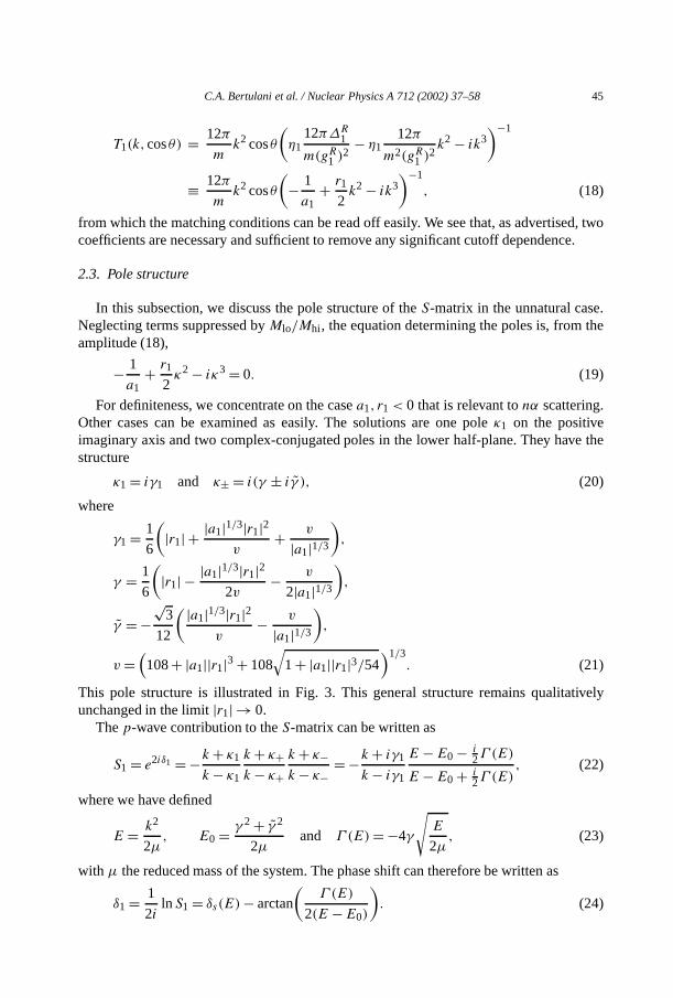
Table 1The values of the scattering lengthal±, the effective rangerl±, and the shape parameterPl± in elasticnα scattering for the 0+, 1−, and 1+ partial waves from Ref. [19]. Thenumbers in parenthesis indicate the error in the last quoted digits. All values are given inunits of the appropriate powers of fm as determined by the orbital angular momentuml

of the partial wave

Partial wavel± al± [fm1+2l ] rl± [fm1−2l ] Pl± [fm3−2l ]

0+ 2.4641(37) 1.385(41) –1− −13.821(68) −0.419(16) –1+ −62.951(3) −0.8819(11) −3.002(62)

from Table 1, we find forMlo 50 MeV from the scattering length and 90 MeV from theeffective range. The average value isMlo ≈ 70 MeV. From the shape parameter, we extractMhi ≈ 260 MeV. This is consistent with the hierarchyMloMhi ∼mπ ∼√mNEα , whereEα = 20.21 MeV is the excitation energy of theα core [21], and suggests that our powercounting is appropriate for the 1+ partial wave. We would expect that the scale of alleffective-range parameters in the remaining channels is set byMhi. Extracting the numbers,however, we find forMhi the scales 80 MeV froma0+, 280 MeV fromr0+, 80 MeV froma1−, and 40 MeV fromr1−. While some spread is not surprising given the qualitativenature of the argument, these numbers suggest that, even though the 1− phase shift issmall, this partial wave might also be dominated byMlo. For the moment we will assumethis is not the case and treat the 1− wave in perturbation theory. We can certainly improveconvergence by resumming 1− contributions. We return to this point in Section 3.4.

3.2. Scattering amplitude in the EFT

A real test of the power counting comes only by calculating the amplitude at variousorders and comparing the results among themselves and with data. In the following, wewill computenα scattering to next-to-leading order in the EFT. For characteristic momentak ∼Mlo, the leading-order contribution to theT -matrix is of order 12π/mMlo. The EFTexpansion is inMlo/Mhi and the NLO and N2LO contributions are suppressed by powersof Mlo/Mhi andM2

lo/M2hi, respectively. The parameters in the effective Lagrangian will

be determined from matching to effective-range parameters. We then compare our resultswith the phase-shift analysis [19] and also directly with low-energy data.

We represent the nucleon and the4He core by a spinor/isospinorN field and ascalar/isoscalarφ field, respectively. We also introduce isospinor dimeron fields that canbe thought of as bare fields for the variousNα channels. In the following we will employs, d , andt , which are spinor, spinor and four-spinor fields associated with thes1/2, p1/2,andp3/2 channels, respectively.

The parity- and time-reversal-invariant Lagrangians for LO and NLO are4

4 We make a particular choice of fields here. TheS-matrix is independent of this choice. One can, for example,redefine thet field so as to remove theg′1+ term. In this case, its contribution (see Eq. (47) below) is reproduced

by a t†Nφ(+ H.c.) interaction with three derivatives.


LLO = φ†[i∂0+

−→∇ 2

2mα

]φ +N†

[i∂0+

−→∇ 2

2mN

]N

+ η1+t†[i∂0+

−→∇ 2

2(mα +mN)−∆1+

]t

+ g1+2

t†S† · [N−→∇φ − (

−→∇N)φ]+H.c.− r

[t†S† · −→∇(Nφ)+H.c.

], (33)

LNLO = η0+s†[−∆0+]s + g0+

[s†Nφ + φ†N†s

]+ g′1+t†[i∂0+

−→∇ 2

2(mα +mN)

]2

t,

(34)

wherer = (mα − mN)/(mα + mN). The notation is analogous to that in Eq. (13). TheSi ’s are the 2× 4 spin-transition matrices connecting states with total angular momentumj = 1/2 andj = 3/2. They satisfy the relations

SiS†j =

2

3δij − i

3εijkσk, S

†i Sj =

3

4δij − 1

6

J

3/2i , J

3/2j

+ i

3εijkJ

3/2k , (35)

where theJ 3/2i are the generators of theJ = 3/2 representation of the rotation group, with[

J3/2i , J

3/2j

]= iεijkJ3/2k . (36)

These Lagrangians generate contributions in the 1+ and 0+ partial waves. There are nocontributions in N2LO, and the 1− partial wave enters first at N3LO.

The propagator for theφ field is

iSφ(p0,p)= i

p0− p2/2mα + iε, (37)

while the nucleon propagator is

iSN(p0,p)abαβ =iδαβδab

p0− p2/2mN + iε. (38)

In Eq. (38),α andβ (a andb) are the incoming and outgoing spin (isospin) indices of thenucleon, respectively. The bare propagator for the 1+ dimeron is

iD01+(p0,p)abαβ =

iη1+δαβδabp0− p2/2(mα +mN)−∆1+ + iε

, (39)

with α andβ (a andb) the incoming and outgoing spin (isospin) indices of the dimeron,respectively. Note thatδαβ is a 4× 4 unit matrix, since the dimeron carriesj = 3/2. Thebare propagator for the 0+ is slightly different because its kinetic terms do not appear untilhigher order:

iD00+(0,0)abαβ =−

iη0+δαβδab∆0+

, (40)

with δαβ now a 2× 2 unit matrix. The bare propagator for the 1− dimeron is the same asfor the 0+ dimeron, with the index 0+ replaced by 1− where appropriate.

The leading contribution to thenα scattering amplitude fork ∼ Mlo is of order12π/mMlo and comes solely from the 1+ partial wave with the scattering-length and


effective-range terms included to all orders. The next-to-leading order correction is sup-pressed byMlo/Mhi and fully perturbative. It consists of the correction from the shape pa-rameterP1+ in the 1+ partial wave and the tree-level contribution of the scattering lengtha0+ in the 0+ partial wave. The 1− partial wave still vanishes at next-to-leading order.

First, we calculate the leading-orderT -matrix elementT LO. As demonstrated forspinless fermions in the previous section, this is most easily achieved by first calculatingthe full dimeron propagator for the 1+ dimeron and attaching the external particle linesin the end. Apart from the spin/isospin algebra, the calculation is equivalent to the onefor spinless fermions that was discussed in detail in the previous section. The proper selfenergy is given by

−iΣ1+(p0,p)abαβ

= g21+∫

ddl

(2π)d

(l− rp/2)i(S†i )βγ (l− rp/2)j (Sj )γ αδab(p0

2 + l0− (p/2+l)22mα

+ iε)(p0

2 − l0− (p/2−l)22mN

+ iε)

=−ig21+(S

†i Sj

)βα

δba

∫dd−1l

(2π)d−1

(l− rp/2)i(l− rp/2)jp0− (p2/4+ l2− rp · l)/2µ+ iε

, (41)

where we have performed thedl0 integral via contour integration. Evaluating the remainingintegral using dimensional regularization with minimal subtraction for simplicity, weobtain

Σ1+(p0,p)abαβ =−δαβδabg2

1+µ6π

[2µ

(−p0+ p2

2(mα +mN)− iε

)]3/2

. (42)

Using Eq. (16), the full dimeron propagator is then given by

iD1+(p0,p)abαβ

= iη1+δαβδab

(p0− p2

2(mα +mN)−∆1+

+ η1+µg21+

6π(2µ)3/2

[−p0+ p2

2(mα +mN)− iε

]3/2

+ iε

)−1

.

(43)

The leading-orderT -matrix element in the center-of-mass system is obtained by setting(p0,p)= (k2/2µ,0) and attaching external particles lines to the full dimeron propagator.This leads to

T LO(k,cosθ) = 2π

µk2(2 cosθ + iσ · n sinθ)

×(η1+

6π∆1+µg2

1+− η1+

6π

µ2g21+

k2

2− ik3

)−1

. (44)

Using Eqs. (2) and (27)–(32), we find the matching conditions

a1+ =−η1+µg2

1+6π∆1+

and r1+ =−η1+6π

µ2g21+

, (45)


which determine the parametersg1+, ∆1+, and the signη1+ in terms of the effective-rangeparametersa1+ andr1+. Then,

F LO(k, θ)= 2k2 cosθ

−1/a1+ + r1+k2/2− ik3 ,

GLO(k, θ)= k2 sinθ

−1/a1+ + r1+k2/2− ik3. (46)

At next-to-leading order, we include all contributions that are suppressed byMlo/Mhicompared to the leading order. These contributions come from the shape parameterP1+and thes-wave scattering lengtha0+. Using the Lagrangian (33) and (34), we find for theT -matrix element:

T NLO = η0+g20+

∆0++ 3πg′1+

2µ3g21+

2π

µ

k6(2 cosθ + iσ · nsinθ)

(−1/a1+ + r1+k2/2− ik3)2. (47)

The first term in Eq. (47) corresponds to the scattering length in the 0+ wave, whilethe second term corresponds to the 1+ amplitude with the shape parameter treated as aperturbation. Using Eqs. (2) and (27)–(32), we find

a0+ =−η0+g2

0+µ2π∆0+

and P1+ =6πg′1+µ3g2

1+. (48)

Note that to this orderη0+, g0+, and∆0+ are not independent and only the combinationappearing in Eq. (48) is determined. The next-to-leading-order pieces ofF andG are then

FNLO(k, θ)=−a0+ + P1+4

2k6 cosθ

(−1/a1+ + r1+k2/2− ik3)2,

GNLO(k, θ)= P1+4

k6 sinθ

(−1/a1+ + r1+k2/2− ik3)2. (49)

3.3. Phase shifts and cross sections in the EFT

In order to see how good our expansion is, we need to fix our parameters. In principle wecould determine the parameters by matching our EFT to the underlying EFT whose degreesof freedom are nucleons (and possibly pions and delta isobars), but no core. Unfortunately,calculations with the latter EFT have not yet reached systems of five nucleons [6]. Forthe time being, we need to determine the parameters from data. For simplicity, we use theeffective-range parameters from Table 1 together with Eqs. (45), (48).

In Fig. 4, we show the phase shifts for elasticnα scattering in the 1+ partial wave as afunction of the neutron kinetic energy in theα rest frame. The filled circles show the phase-shift analysis of Ref. [19]. The dashed line shows the EFT result at leading order. The LOresult already shows a good agreement with the full phase-shift analysis. As expected,the agreement deteriorates with energy. NLO corrections improve the agreement: the EFTresult at NLO shown by the solid line reproduces the phase-shift analysis exactly. If betterdata were available and a more complete phase-shift analysis were performed, some smalldiscrepancies would survive, to be remedied by higher orders.


Fig. 4. The phase shift fornα scattering in the 1+ partial wave as a function of the neutron kinetic energy in theα rest frame. The dashed (solid) line shows the EFT result at LO (NLO). The filled circles show the phase-shiftanalysis [19] which the EFT at NLO reproduces exactly. The dotted line shows the contribution of the scatteringlength alone.

The sharp rise in the 1+ phase shift pastπ/2 denotes the presence of a resonance.To LO, the pole structure of theS-matrix is given in Section 2.3. We findγ1 = 99 MeV,γ = −6 MeV, andγ = 34 MeV. Using Eq. (23), the position and width of the resonanceareE0= 0.8 MeV andΓ (E0)= 0.6 MeV, respectively. The two virtual states that producethe resonance are indeed at|k| ∼ Mlo. The real bound state, for reasons that cannotbe understood from the EFT itself, turns out numerically to be at considerably highermomentum, where the EFT can no longer be trusted. This is consistent with the knownabsence of a real5He bound state.

We also illustrate in Fig. 4 an important aspect of the power counting. The dottedline shows the result from iteratingCp

2 alone. In other words, it is the contribution ofthe scattering length only. This curve, which would come from a naive application of thepower counting fors-waves [9,10], does not correspond to any order in the power countingdeveloped here, and clearly fails to describe the resonance nearEn = 1 MeV.

In Fig. 5, we show the phase shifts for elasticnα scattering in the 0+ partial wave asa function of the neutron kinetic energy in theα rest frame. In LO the phase shift is zero.The solid line shows the EFT result at next-to-leading order. The NLO result already showsgood agreement with the full phase-shift analysis [19], depicted by the filled circles.

The phase shifts in the 1− and all other partial waves are identically zero to NLO. Thefirst non-zero contribution appears at N3LO in the 1− channel. All other waves appear ateven higher orders. That they are indeed very small one can conclude from their absencein the phase-shift analysis [19].

Obviously, not all partial waves are treated equally in our power counting. In orderto further assess if the power counting is appropriate, we compare the EFT predictionsdirectly to some observables. In Fig. 6, we compare the EFT predictions with data for the


Fig. 5. The phase shift fornα scattering in the 0+ partial wave as a function of the neutron kinetic energy in theα rest frame. The solid line shows the EFT result at NLO; at LO this phase shift is zero. The filled circles showthe result of the phase-shift analysis [19].

total cross section as a function of the neutron kinetic energy in theα rest frame. Thediamonds are “evaluated data points” from Ref. [22]. In order to have an idea of the errorbars from individual experiments we also show data from Ref. [23] as the black squares.The dashed line shows the EFT result at LO which already gives a fair description ofthe resonance region but underestimates the cross section at threshold. The NLO resultgiven by the solid curve gives a good description of the cross section from threshold up toenergies of about 4 MeV.

We can also calculate other observables. As another example, we show in Fig. 7the center-of-mass differential cross section at a momentumkCM = 49.6 MeV. (Thiscorresponds to a neutron kinetic energyEn = 2.05 MeV in theα rest frame.) The diamondsare evaluated data from Ref. [22].5 The dashed line shows the EFT results at LO, whichis purep-wave. At NLO, shown as a solid line, interference with thes-wave term givesessentially the correct shape.

If we carry out the EFT to a sufficiently high order, we will have included all terms usedin the phase-shift analysis [19], and more. At this order, the high quality of our fit is purelya consequence of the high quality of that fit. Note, however, that this is by no means true atthe lower orders explicitly displayed above. In particular, it is perhaps surprising that our1− wave does not appear until relatively high order. The fact that the EFT converges fast todata shows that the power counting developed here is reasonable. The 1− wave is furtherdiscussed in the next section.

5 In order to obtain the differential cross section from the NNDC neutron emission spectra we divide by 2π

and multiply by the total cross section.


Fig. 6. The total cross section fornα scattering in barns as a function of the neutron kinetic energy in theα

rest frame. The diamonds are evaluated data from Ref. [22], and the black squares are experimental data fromRef. [23]. The dashed and solid lines show the EFT results at LO and NLO, respectively. The dash-dotted lineshows the LO result in the modified power counting where the 1− partial wave is promoted to leading order.

Fig. 7. The differential cross section fornα scattering in the center-of-mass frame in barn/sr as a function of thescattering angleθCM at a momentumkCM = 49.6 MeV. The diamonds are evaluated data from Ref. [22]. Thedashed and solid lines show the EFT results at LO and NLO, respectively. The dash-dotted line shows the LOresult in the modified power counting where the 1− partial wave is promoted to leading order.


3.4. Further discussion of the power counting

As we have shown, the EFT describes the data pretty well at least up toEn = 4 MeVor so. One way to improve the convergence at higher energies is to take the scale of non-perturbative phenomena in the 1− wave as a low scale. We can modify the power countingand count the 1− parameters the same as the 1+ parameters. The LO Lagrangian fromEq. (33) then has an additional term

LALO = η1−d†[i∂0+

−→∇ 2

2(mα +mN)−∆1−

]d

+ g1−2

d†σ † · [N−→∇φ − (

−→∇N)φ]+H.c.− r

[d†σ † · −→∇(Nφ)+H.c.

].

(50)

The calculation of theT -matrix for the 1− partial wave proceeds exactly as for the 1+partial wave. The amplitudesF andG acquire the following additional contributions atleading order

FALO(k, θ)= k2 cosθ

−1/a1− + r1−k2/2− ik3 ,

GALO(k, θ)=− k2 sinθ

−1/a1− + r1−k2/2− ik3. (51)

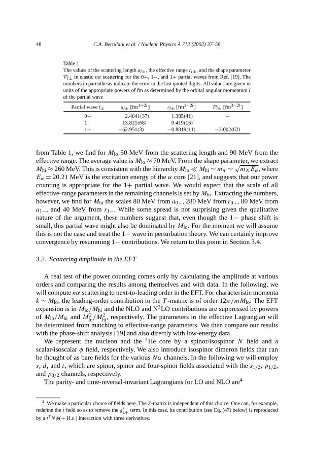
In Fig. 8, we show the phase shifts fornα scattering in the 1− partial wave obtainedin this alternative power counting. The filled circles show the result of the partial-wave analysis of Ref. [19] which is exactly reproduced by the leading-order EFT withthe modified power counting given by the dash-dotted line. The dotted line shows thecontribution of the scattering length only. The next-to-leading order in the modifiedcounting cannot be easily computed at present becauseP1− is not known.

The cross sections corresponding to the leading order in the modified power countingare shown by the dash-dotted curve in Figs. 6 and 7. In the total cross section, promotingthe 1− partial wave to leading order gives almost no improvement compared to the originalcounting except at higher energies, but even there the NLO result in the original countinggives better results. In the differential cross section atkCM = 49.6 MeV (corresponding toEn = 2.05 MeV in theα rest frame), the alternative power counting gives no improvementover the LO result (compare the dashed and dash-dotted lines in Fig. 7). We did notfind a significant improvement in the differential cross section over the leading order bypromoting the 1− partial wave for neutron energies up toEn ≈ 4 MeV. For reproducingthe differential cross section, the interference betweens1/2- andp3/2-waves is much moreimportant than the additionalp1/2 contribution. As a consequence, we deem the originalpower counting most appropriate for elasticnα scattering atk ∼Mlo.

Finally, note that fork Mlo the power counting has to discriminate betweenmomentumk and the low-energy scaleMlo. Thep-waves, for example, die faster thanthes-waves. That is the reason our results for the cross section in this region are not gooduntil we get to NLO. It is easy to adapt the power counting forkMlo: in fact, the fullamplitude—all waves, that is—can be treated in perturbation theory, as in Section 2.1. Formore details, see Ref. [9].


Fig. 8. The phase shift fornα scattering in the 1− partial wave as a function of the neutron kinetic energy intheα rest frame. The filled circles show the result of the phase-shift analysis [19] which is exactly reproducedby leading-order EFT with the modified power counting given by the dash-dotted line. The dotted line shows thecontribution of the scattering length only.

4. Conclusion and outlook

In this paper we have examined the problem of the interaction between a neutron andan α particle at low energies. We showed that a power counting can be formulated thatleads to consistent renormalization. In leading order, two interactions have to be fullyiterated. These two interactions generate a shallowp3/2-wave resonance near the observedenergy and width. In subleading orders the phase shifts in all waves can be systematicallyimproved. Observables calculated directly are very well reproduced.

The crucial ingredient for the applicability of the EFT to bound states and resonancesof halo type is their low characteristic energies. In this sense, the deuteron can be thoughtof as the simplest halo nucleus whose core is a nucleon.nα scattering plays an analogousrole here asnp plays in the nucleons-only EFT. It is clear now how to extend the EFTto more complicated cores: one simply introduces an appropriate field for the core underconsideration, extends the power counting to the relevant channels, and determines thestrength of interactions order-by-order from data.

With the parameters of the nucleon–core interaction fixed in lowest orders, we canproceed to more-body halos. The simplest example is6He. In addition to thenα interaction,thenn interaction has also been determined from data.6He, like the triton, can be describedas a three-body system of a core and two neutrons. The role of a three-body interaction canbe addressed by renormalization group techniques [13,18].

Note that the EFT approach is by no means restricted to neutron halos. The Coulombinteraction can be included in the same way as in the nucleons-only sector [24], allowing


for the analysis of nuclei such as8B. Radiative capture on halo nuclei, such asp+ 7Be→8B+ γ , can then be calculated much liken+ p→ d + γ .

Our approach is not unrelated to traditional single-particle models. In the latter, thenucleon–core interaction is frequently parametrized by a simple potential with centraland spin-orbit components [25]. The parameters of the potential are adjusted to reproducewhatever information is accessible experimentally. In the EFT, we make the equivalent toa multipole expansion of the underlying interaction. The spin–orbit splitting, in particular,results from the different parameters of the dimeron fields with different spins. In the EFTthe nucleon–nucleon interaction is treated in the same way as the nucleon–core interaction,mutatis mutandis. ContactNN interactions have in fact already been used in the studyof Borromean halos [26]. It was found that density dependence, representing three-body effects, needed to be added in order to reproduce results from more sophisticatedparametrizations of theNN interaction. In the EFT, the need for an explicit three-bodyforce can be decided on the basis of the renormalization group before experiment isconfronted. A zero-range model with purelys-waveNN and nucleon–core interactionswas examined in Ref. [27].

The EFT unifies single-particle approaches in a model-independent framework, with theadded power counting that allows for an a priori estimate of errors. It also casts halo nucleiwithin the same framework now used to describe few-nucleon systems consistently withQCD [6,8]. Therefore, the EFT with a core can in principle be matched to the underlying,nucleons-only EFT. Nuclei near the drip lines open an exciting new field for the applicationof EFT ideas. It remains to be seen, however, whether these developments will prove to bea significant improvement over more traditional approaches.

Acknowledgements

We would like to thank Martin Savage for an interesting question, and Henry Weller andRon Tilley for help in unearthingnα scattering data. H.-W.H. and U.v.K. are grateful to theKellogg Radiation Laboratory of Caltech for its hospitality, and to RIKEN, BrookhavenNational Laboratory and to the US Department of Energy (DE-AC02-98CH10886) forproviding the facilities essential for the completion of this work. This research wassupported in part by the National Science Foundation under Grant No. PHY-0098645(H.-W.H.) and by a DOE Outstanding Junior Investigator Award (U.v.K.).

References

[1] B.A. Brown, A. Csótó, R. Sherr, Nucl. Phys. A 597 (1996) 66;H. Esbensen, G.F. Bertsch, Nucl. Phys. A 600 (1996) 37.

[2] M.V. Zhukov, B.V. Danilin, D.V. Fedorov, J.M. Bang, I.J. Thompson, J.S. Vaagen, Phys. Rep. 231 (1993)151;K. Riisager, Rev. Mod. Phys. 66 (1994) 1105.

[3] Scientific opportunities with fast fragmentation beams from RIA, NSCL-report, March 2000.[4] C.A. Bertulani, M.S. Hussein, G. Münzenberg, Physics of Radioactive Beams, Nova Science Publishers,

Huntington, NY, 2002.


[5] G.P. Lepage, in: T. De Grand, D. Toussaint (Eds.), From Actions to Answers, TASI’89, World Scientific,Singapore, 1990;D.B. Kaplan, nucl-th/9506035.

[6] P.F. Bedaque, U. van Kolck, nucl-th/0203055, Annu. Rev. Nucl. Part. Sci., in press;S.R. Beane, P.F. Bedaque, W.C. Haxton, D.R. Phillips, M.J. Savage, in: M. Shifman (Ed.), Boris IoffeFestschrift, World Scientific, Singapore, 2001.

[7] P.F. Bedaque, M.J. Savage, R. Seki, U. van Kolck (Eds.), Nuclear Physics with Effective Field Theory II,World Scientific, Singapore, 1999;R. Seki, U. van Kolck, M.J. Savage (Eds.), Nuclear Physics with Effective Field Theory, World Scientific,Singapore, 1998.

[8] S. Weinberg, Phys. Lett. B 251 (1990) 288;S. Weinberg, Nucl. Phys. B 363 (1991) 3;M. Rho, Phys. Rev. Lett. 66 (1991) 1275;C. Ordóñez, U. van Kolck, Phys. Lett. B 291 (1992) 459.

[9] U. van Kolck, in: A. Bernstein, D. Drechsel, T. Walcher (Eds.), Proceedings of the Workshop on ChiralDynamics 1997, Theory and Experiment, Springer, Berlin, 1998, hep-ph/9711222;U. van Kolck, Nucl. Phys. A 645 (1999) 273.

[10] D.B. Kaplan, M.J. Savage, M.B. Wise, Phys. Lett. B 424 (1998) 390;D.B. Kaplan, M.J. Savage, M.B. Wise, Nucl. Phys. B 534 (1998) 329.

[11] J.-W. Chen, G. Rupak, M.J. Savage, Nucl. Phys. A 653 (1999) 386;S.R. Beane, M.J. Savage, Nucl. Phys. A 694 (2001) 511.

[12] J.-W. Chen, M.J. Savage, Phys. Rev. C 60 (1999) 065205;G. Rupak, Nucl. Phys. A 678 (2000) 405.

[13] P.F. Bedaque, H.-W. Hammer, U. van Kolck, Phys. Rev. Lett. 82 (1999) 463;P.F. Bedaque, H.-W. Hammer, U. van Kolck, Nucl. Phys. A 646 (1999) 444.

[14] P.F. Bedaque, U. van Kolck, Phys. Lett. B 428 (1998) 221;P.F. Bedaque, H.-W. Hammer, U. van Kolck, Phys. Rev. C 58 (1998) R641;F. Gabbiani, P.F. Bedaque, H.W. Grießhammer, Nucl. Phys. A 675 (2000) 601.

[15] P.F. Bedaque, H.-W. Hammer, U. van Kolck, Nucl. Phys. A 676 (2000) 357;H.-W. Hammer, T. Mehen, Phys. Lett. B 516 (2001) 353.

[16] H.-W. Hammer, Nucl. Phys. A 705 (2002) 173.[17] D.V. Fedorov, A.S. Jensen, Nucl. Phys. A 697 (2002) 783.[18] C.A. Bertulani, H.-W. Hammer, U. van Kolck, in preparation.[19] R.A. Arndt, D.L. Long, L.D. Roper, Nucl. Phys. A 209 (1973) 429.[20] D.B. Kaplan, Nucl. Phys. B 494 (1997) 471.[21] D.R. Tilley, H.R. Weller, G.M. Hale, Nucl. Phys. A 541 (1992) 1.[22] Evaluated Nuclear Data Files, National Nuclear Data Center, Brookhaven National Laboratory,

http://www.nndc.bnl.gov/.[23] B. Haesner, et al., Phys. Rev. C 28 (1983) 995;

M.E. Battat, et al., Nucl. Phys. 12 (1959) 291.[24] X. Kong, F. Ravndal, Nucl. Phys. A 665 (2000) 137.[25] S. Ali, A.A.Z. Ahmad, N. Ferdous, Rev. Mod. Phys. 57 (1985) 923.[26] G.F. Bertsch, H. Esbensen, Ann. Phys. 209 (1991) 327;

H. Esbensen, G.F. Bertsch, K. Hencken, Phys. Rev. C 56 (1997) 3054.[27] A.E.A. Amorim, T. Frederico, L. Tomio, Phys. Rev. C 56 (1997) R2378;

A. Delfino, T. Frederico, M.S. Hussein, L. Tomio, Phys. Rev. C 61 (2000) 051301.

http://www.nndc.bnl.gov/

Documents

Effective ﬁeld theory for halo nuclei: shallow p-wave …faculty.tamuc.edu/cbertulani/cab/papers/NPA_712_37.pdfEffective ﬁeld theory for halo nuclei: shallow p-wave states C.A