Embed Size (px)
Citation preview
EFFECTIVE EQUIDISTRIBUTION AND THE SATO-TATE LAW FORFAMILIES OF ELLIPTIC CURVES
STEVEN J. MILLER AND M. RAM MURTY
ABSTRACT. Extending recent work of others, we provide effective bounds on the fam-ily of all elliptic curves and one-parameter families of elliptic curves modulo p (for pprime tending to infinity) obeying the Sato-Tate Law. We present two methods of proof.Both use the framework of Murty-Sinha [MS]; the first involves only knowledge of themoments of the Fourier coefficients of the L-functions and combinatorics, and saves alogarithm, while the second requires a Sato-Tate law. Our purpose is to illustrate howthe caliber of the result depends on the error terms of the inputs and what combinatoricsmust be done.
1. INTRODUCTION
Recently M. Ram Murty and K. Sinha [MS] proved effective equidistribution resultsshowing the eigenvalues of Hecke operators on the space S(N, k) of cusp forms ofweight k and level N agree with the Sato-Tate distribution. Our goal here is to use theirframework to prove similar results for families of elliptic curves. We shall do this forthe family of all elliptic curves and for one-parameter families of elliptic curves.
We first review notation and previous results. Let E : y2 = x3 + Ax + B withA,B ∈ ℤ be an elliptic curve over ℚ with associated L-function
L(E, s) =∞∑n=1
aE(n)
ns=
∏p
(1− aE(p)
ps+
Â0(p)
p2s−1
)−1
, (1.1)
2000 Mathematics Subject Classification. 11H05 (primary) 11K38, 14H52, 11M41 (secondary).Key words and phrases. Sato-Tate, Elliptic Curves, Erdös-Turan, Effective Equidistribution.The authors would like to thank Andrew Granville for pointing out the implicit normalization in
Birch’s work, Igor Shparlinski for discussions on previous results as well as sharing his recent work,and Frederick Strauch for conversations on a hypergeometric proof of Lemma A.3; the first named au-thor would also like to thank Cameron and Kayla Miller for quietly sleeping on him while many of thecalculations were done. Much of this paper was written when the authors attended the Graduate Work-shop on L-functions and Random Matrix Theory at Utah Valley University in 2009, and it is a pleasureto thank the organizers. The first named author was partly supported by NSF grants DMS0600848 andDMS0970067. The second named author was partially supported by an NSERC Discovery grant.
1
2 STEVEN J. MILLER AND M. RAM MURTY
where Δ = −16(4A3 + 27B2) is the discriminant of E, Â0 is the principal charactermodulo Δ, and
aE(p) = p−#{(x, y) ∈ (ℤ/pℤ)2 : y2 ≡ x3 + Ax+B mod p}= −
∑
x mod p
(x3 + Ax+B
p
). (1.2)
By Hasse’s bound we know ∣aE(p)∣ ≤ 2√p, so we may write aE(p) = 2
√p cos µE(p),
where we may choose µE(p) ∈ [0, ¼]. See [Sil1, Sil2, ST] for more details and proofsof all the needed properties of elliptic curves.
How the aE(p)’s vary is of great interest. One reason for this is that they encodelocal data (the number of solutions modulo p), and are then combined to build the L-function, whose properties give global information about E. For example, the Birch andSwinnerton-Dyer conjecture [BS-D1, BS-D2] states the order of the group of rationalsolutions of E equals the order of vanishing of L(E, s) at the central point. While weare far from being able to prove this, the evidence for the conjecture is compelling,especially in the case of complex multiplication and rank at most 1 [Bro, CW, GKZ,GZ, Kol1, Kol2, Ru]. In addition there is much suggestive numerical evidence for theconjecture; for example, for elliptic curves with modest geometric rank r, numericalapproximations of the first r−1 Taylor coefficients are consistent with these coefficientsvanishing (see for instance the families studied in [Fe1, Fe2, Mil3]).
If E has complex multiplication1 then aE(p) = 0 for half the primes; i.e., µE(p) =¼/2. The remaining angles µE(p) are uniformly distributed in [0, ¼] (this follows from[Deu, He1, He2]).
If E does not have complex multiplication, which is the case for most elliptic curves,then Sato and Tate [Ta] conjectured that as we vary p, the distribution of the µE(p)’sconverges to 2 sin2 µdµ/¼. More precisely, for any interval I ⊂ [0, ¼] we have
limx→∞
#{p : p ≤ x : µE(p) ∈ I}#{p : p ≤ x} =
∫
I
2 sin2 µdµ
¼; (1.3)
we call 2 sin2 µdµ/¼ the Sato-Tate measure, and denote it by ¹ST. By recent results ofClozel, Harris, Shepherd-Barron and Taylor [CHT, HS-BT, Tay], this is now knownfor all such E that have multiplicative reduction at some prime; see also [BZ] for re-sults on the error terms when ∣I∣ is small (these results are not for an individual curve,but rather averaged over the family of all elliptic curves) and [B-LGG, B-LGHT] forgeneralizations to other families of L-functions.
Instead of fixing an elliptic curve and letting the prime vary, we can instead fix aprime p and study the distribution of µE(p) as we vary E. Before describing our results,we briefly summarize related results in the literature concerning Sato-Tate behavior in
1This means the endomorphism ring is larger than the integers. For example, y2 = x3−x has complexmultiplication, as can be seen by sending (x, y) → (−x, iy). Note aE(p) = 0 if p ≡ 3 mod 4 (this canbe seen from the definition of aE(p) as a sum of Legendre symbols, sending x → −x).
EFFECTIVE EQUIDISTRIBUTION AND SATO-TATE FOR ELLIPTIC CURVES 3
families. Serre [Ser] considered a similar question, not for elliptic curves, but rather forS(N, k), the space of cusp forms of weight k on Γ0(N). He proved that for even k withN + k → ∞ the eigenvalues of the normalized pth Hecke operators are equidistributedin [−2, 2] with respect to the measure
¹p =p+ 1
¼
√1− x2/4 dx
(p1/2 + p−1/2)2 − x2; (1.4)
changing variables by setting x = 2 cos µ this is equivalent to the measure ¹p on [0, ¼]given by
¹p =2(p+ 1)
¼
sin2 µdµ
(p1/2 + p−1/2)2 − 4 cos2 µ. (1.5)
Note that as p → ∞, ¹p → ¹ST; for p large these two measures assign almost the sameprobability to an interval I , differing by O(1/p). See [CDF, Sar] for other families witha similar distribution.
Serre’s theorem was ineffective, and has recently been improved by M. R. Murty andK. Sinha [MS]. They show that if {an(p)/p(k−1)/2}1≤i≤#S(N,k) denote the normalizedeigenvalues of the Hecke operator Tp on S(N, k), then
#{1 ≤ n ≤ N : an(p)/p(k−1)/2 ∈ I}
#S(N, k)=
∫
I
¹p +O
(log p
log kN
), (1.6)
where #S(N, k) is the number of cusp forms of weight k and level N , and if N ≥ 61then by Corollary 15 of [MS] we have
3Ã(N)
200≤ #S(N, k) ≤ Ã(N)
12+ 1, (1.7)
where Ã(N) = N∏
p∣N(1 + 1
p
). This effective version of equidistribution allows
Murty and Sinha to derive many results, such as
∙ an effectively computable constant Bd such that if J0(N) (the Jacobian of themodular curve X0(N)) is isogenous to a product of ℚ-simple abelian varietiesof dimensions at most d, then N ≤ Bd;
∙ the multiplicity of any given eigenvalue of the Hecke operators is ≪ s(N,k) log plog kN
.
The purpose of this paper is to expand the techniques in [MS] to families of ellipticcurves. Unlike [MS, Ser], we cannot keep the prime fixed throughout the argument, asthere are only finitely many distinct reductions of elliptic curves modulo p. Instead wefix a prime and study the angles µE(p) for one of the two families below, and then sendp → ∞. We study
(1) The family of all elliptic curves modulo p for p ≥ 5. We may write these curvesin Weierstrass form as y2 = x3 − ax− b with a, b ∈ ℤ/pℤ and 4a3 ∕= 27b2. The
4 STEVEN J. MILLER AND M. RAM MURTY
number of pairs (a, b) satisfying these conditions2 is p(p− 1).
(2) One-parameter families over ℚ(T ): let A(T ), B(T ) ∈ ℤ[T ] and consider thefamily y2 = x3 + A(T )x + B(T ) with non-constant j(T ).3 We specialize Tto be a t ∈ ℤ/pℤ. The cardinality of the family is p + OA,B(1) (we lose afew values when we specialize as we require the reduced curves to be ellipticcurves modulo p), where the error is a function of the discriminant of the family.
Notations:∙ We let ℱp denote either family, and write Vp for its cardinality (which is p(p−1)
in the first case and p+O(1) in the second).
∙ While we may denote the angles by µE(p), µa,b(p) or µt(p), as p is fixed for no-tational convenience and to unify the presentation we shall denote these by µn,with 1 ≤ n ≤ Vp.
∙ We let e(x) = e2¼ix.
Normalizations:
∙ For the family of all elliptic curves, we may match the elliptic curves in pairs(E,E ′) such that µE′(p) = ¼ − µE(p) (and each curve is in exactly one pair);see Remark 1.1 for a proof. Thus, if we let xn = µn(p)/¼, we see that the set{2xn}n≤Vp is symmetric about ¼. This will be very important later, as it means∑
n≤Vpsin(2¼mxn) = 0 for any integer m.
∙ For a one-parameter family of elliptic curves, in general we cannot match the el-liptic curves in pairs, and thus the set {2µt(p)} is not typically symmetric about¼; see Remark 1.2 for some results about biases in the µt(p)’s. This leads tosome complications in proving equidistribution, as certain sine terms no longervanish. To overcome this, following other researchers we consider the techni-cally easier situation where for each elliptic curve we include both µt(p) and2¼ − µt(p). To unify the presentation, instead of normalizing these angles bydividing by 2¼ (to obtain a distribution supported on [0, 1]), we first study theangles modulo ¼ and then divide by ¼. We thus consider the normalized anglesxt = µt(p)/¼ and xt+Vp = 1 − µt(p)/¼ for 1 ≤ t ≤ Vp. Thus we study 2Vp
2If a = 0 then the only b which is eliminated is b = 0. If a is a non-zero perfect square there are twob that fail, while if a is not a square than no b fail. Thus the number of bad pairs of (a, b) is p.
3Up to constants, j(T ) is A(T )3/(4A(T )3 + 27B(T )2).
EFFECTIVE EQUIDISTRIBUTION AND SATO-TATE FOR ELLIPTIC CURVES 5
normalized angles in [0, 1], unlike the case of all elliptic curves where we hadVp angles.
∙ We set Vp = Vp for the family of all elliptic curves, and 2Vp for a one-parameterfamily of elliptic curves. We study the distribution of the normalized angles{xn}1≤n≤Vp
.
Remark 1.1. To see that we may match the angles as claimed for the family of allelliptic curves, consider the elliptic curve y2 = x3 − ax − b with 4a3 ∕= 27b2. Let c beany non-residue modulo p, and consider the curve y2 = x3 − ac2x − bc3. Using theLegendre sum expressions for aE(p) and aE′(p), using the automorphism x → cx wesee the second equals
(cp
)times the first; as we have chosen c to be a non-residue, this
means 2√p cos(µE′(p)) = −2
√p cos(µE(p)), or µE′(p) = ¼ − µE(p) as claimed.
Remark 1.2. If the one-parameter family of elliptic curves has rank r over ℚ(T ) andsatisfies Tate’s conjecture (see [Ta, RS]), then Rosen and Silverman [RS] prove a con-jecture of Nagao [Na], which states
limX→∞
− 1
X
∑p≤X
A1(p) log p
p= r (1.8)
where A1(p) :=∑
t mod p at(p). Tate’s conjecture is known for rational surfaces.4 Thisbias has been used by S. Arms, Á. Lozano-Robledo and S. J. Miller [AL-RM] to con-struct one-parameter families with moderate rank by finding families where A(p) isessentially −rp. As there are about p curves modulo p, this represents a bias of about−r on average per curve; as each at(p) is of order
√p, we see in the limit that this bias
should be quite small per curve (though significant enough to lead to rank, it gives alower order contribution to the distribution for each prime, and will be dwarfed by ourother errors).
Our goal is to prove effective theorems on the rate of convergence as p → ∞ to theSato-Tate measure, which requires us to obtain effective estimates for∣∣∣#{n ≤ Vp : µn ∈ I} − ¹ST(I)Vp
∣∣∣ . (1.9)
Here ¹ST is the Sato-Tate measure on [0, ¼] given by
¹ST(T ) =
∫
I
2
¼sin2 tdt I ⊂ [0, ¼], (1.10)
4An elliptic surface y2 = x3 + A(T )x + B(T ) is rational if and only if one of the following is true:(1) 0 < max{3degA, 2degB} < 12; (2) 3degA = 2degB = 12 and ordt=0t
12Δ(t−1) = 0.
6 STEVEN J. MILLER AND M. RAM MURTY
and for n ≤ Vp, 2√p cos(µn) is the number of solutions modulo p of the elliptic curve
En : y2 = x3 + anx+ bn. Equivalently, using the normalization xn = µn/¼ to obtain adistribution on [0, 1], the Sato-Tate measure become
¹st(I) =
∫
I
2 sin2(¼x)dx, I ⊂ [0, 1]. (1.11)
For a sequence of numbers xn modulo 1, a measure ¹ and an interval I ⊂ [0, 1], let
NI(Vp) = #{n ≤ Vp : xn ∈ I}¹(I) =
∫
I
¹(t)dt. (1.12)
The discrepancy DI,Vp(¹) is
DI,Vp(¹) =
∣∣∣NI(Vp)− Vp¹(I)∣∣∣ , (1.13)
and trivially DI,Vp(¹) ≤ Vp. The goal is to obtain the best possible estimate for how
rapidly DI,Vp(¹)/Vp tends to 0.
Previous work has obtained a power savings in convergence to Sato-Tate for two-parameter families of elliptic curves (such as the entire family of all elliptic curves, orparametrizations such as y2 = x3 + f(a)x + g(b) with a and b varying in appropriateranges); see the papers by Banks and Shparlinski [BS, Sh1, Sh2] for saving V
1/4p in
Sato-Tate convergence. The key step in these arguments is1
(p− 1)2
∑a,b mod p
4a3+27b2 ∕≡0 mod p
sin((k + 1)µa,b(p))
sin(µa,b(p)≪ kp−1/2, k = 1, 2, . . . ; (1.14)
see Theorem 13.5.3 from [Ka] for a proof. One can obtain new and similar resultsfor one-parameter families of elliptic curves by appealing to a result of Michel [Mic],which we do in §4. Our main results are the following.
Theorem 1.3 (Family of all curves). For the family of all elliptic curves modulo p, asp → ∞ we have
DI,Vp(¹st) ≤ C
Vp
log Vp
(1.15)
for some computable C. Note that in this family, Vp = Vp and for each curve we includeone normalized angle, xn = µn/¼ ∈ [0, 1].
Theorem 1.4 (One-parameter family of elliptic curves). For a one-parameter family ofelliptic curves over ℚ(T ) with non-constant j-invariant, we have
DI,Vp(¹st) ≤ CV 3/4
p (1.16)
for some computable C. Note that in this family, Vp = 2Vp and for each curve weinclude two normalized angles, xn = µn/¼ and xn+Vp = 1− µn/¼, with µn ∈ [0, ¼].
EFFECTIVE EQUIDISTRIBUTION AND SATO-TATE FOR ELLIPTIC CURVES 7
Stronger results than Theorem 1.3 are known; as remarked above, convergence toSato-Tate with an error of size V
3/4p instead of Vp/ log Vp is obtained in [BS, Sh1, Sh2].
We present these weaker arguments to highlight how one may attack these problemspossessing only knowledge of the moments, and not the functions of the angles, inthe hope that these arguments might be of use to other researchers attacking similarquestions where we only have formulas for the moments of the coefficients. We willthus illustrate the effectiveness (in both senses of the word) of the techniques in [MS],as well as illustrate the loss of information that comes from having to trivially boundcertain combinatorial sums. As we have not found similar effective results in the liter-ature for one-parameter families, in order to get the best possible results we do not useformulas for the moments but rather estimates for the analogue of (1.14). It is worth re-marking that we can recover the results of [BS, Sh1, Sh2] by our generalization of [MS]provided we also use (1.14) (see [Ka]) instead of results from Birch [Bi] on moments;this shows the value of the formulation in [MS].
We summarize the key ingredients of the proofs, and discuss why the second resulthas a much better error term than the first. Similar to [MS], both theorems followfrom an analysis of
∑n≤Vp
e(mxn) (we use xn = µn/¼ in order to have a distributionsupported on [0, 1]). For the family of all elliptic curves, after some algebra we see thisis equivalent to understanding
∑n≤Vp
cos(2mµn); using a combinatorial identity (see[Mil4]) this is equivalent to a linear combination of sums of the form
∑n≤Vp
(cos µn)2r.
These sums are essentially the 2rth moments of the Fourier coefficients of the family ofall elliptic curves modulo p. Birch [Bi] evaluated these, and showed the answers are theCatalan numbers5 plus lower order terms. Our equidistribution result then follows froma combinatorial identity of a sum of weighted Catalan numbers; our error term is poordue to the necessity of losing cancelation in bounding the contribution from the sumsof the error terms.
The proof of Theorem 1.4 is easier, as now instead of inputting results on the mo-ments we instead use a result of Michel [Mic] for the sum over the family of symk(µn) =sin((k + 1)µn)/ sin µn. This is easily related to our quantity of interest, cos(2mµn),through identities of Chebyshev polynomials:
cos(2mµn) =1
2sym2m(µn)−
1
2sym2m−2(µn). (1.17)
The advantage of having a formula for the quantity we want and not a related quantityis that we avoid trivially estimating the errors in the combinatorial sums. These cal-culations increased the size of the error significantly, and this is why Theorem 1.4 isstronger than Theorem 1.3, though the error term in Theorem 1.3 is comparable to the
5The Catalan numbers are the moments of the semi-circle distribution, which is related to the Sato-Tatedistribution through a simple change of variables.
8 STEVEN J. MILLER AND M. RAM MURTY
error terms of the equivalent quantities in [MS] for the family of cuspidal newforms.Michel proves his result by using a cohomological interpretation, and this results in theerror term being p−1/2 smaller than the main term; it is this savings in the quantity weare directly interested in that leads to the superior error estimates.
The paper is organized as follows. After reviewing the needed results from Murty-Sinha [MS] in §2, we prove Theorem 1.3 in §3 and Theorem 1.4 in §4. For completenessthe needed combinatorial identities are proved in Appendix A, and in Appendix B wecorrect some errors in explicit formulas for moments in Birch’s paper [Bi] (where heneglected to mention that his sums are normalized by dividing by p− 1).
2. EFFECTIVE EQUIDISTRIBUTION PRELIMINARIES
We quickly review some needed results from Murty-Sinha [MS]; while our settingis similar to the problems they investigated, there are slight differences which requiregeneralizations of some of their results. Assume ¹ = F (−x)dx with
F (x) =∞∑
m=−∞cme(mx) (2.1)
where e(z) = exp(2¼iz). Theorem 8 from [MS] is
Theorem 2.1. Let {xn} be a sequence of real numbers in [0, 1] and let the notation beas above. Assume for each m that
limVp→∞
1
Vp
∑
n≤Vp
e(mxn) = cm and∞∑
m=−∞∣cm∣ < ∞. (2.2)
Let ∣∣¹∣∣ = supx∈[0,1] ∣F (x)∣ with ¹ = F (−x)dx. Then the discrepancy satisfies
DI,Vp(¹) ≤ Vp∣∣¹∣∣
M + 1
+∑
1≤m≤M
(1
M + 1+min
(b− a,
1
¼∣m∣)) ∣∣∣∣∣∣
Vp∑n=1
e(mxn)− Vpcm
∣∣∣∣∣∣(2.3)
for any natural numbers Vp and M .
Unfortunately, Theorem 2.1 is not directly applicable in our case. The reason is thatthere we have a limit as Vp → ∞ in the definition of the cm, where for us we fix a primep and have Vp = p(p−1) for the family of all elliptic curves curves modulo p, or p+O(1)for a one-parameter family. Analyzing the proof of Theorem 8 from [MS], however, wesee that the claim holds for any sequence cm (obviously if V −1
p
∑n≤Vp
e(mxn) is notclose to cm then the discrepancy is large). We thus obtain
EFFECTIVE EQUIDISTRIBUTION AND SATO-TATE FOR ELLIPTIC CURVES 9
Theorem 2.2. Let {xn} be a sequence of real numbers in [0, 1] and let the notation beas above. Let {cm} be a sequence of numbers such that
∑∞m=−∞ ∣cm∣ < ∞ (we will
take c0 = 1, c±1 = −1/2 and all other cm’s equal to zero). Let ∣∣¹∣∣ = supx∈[0,1] ∣F (x)∣with ¹ = F (−x)dx. Then the discrepancy satisfies
DI,Vp(¹) ≤ Vp∣∣¹∣∣
M + 1
+∑
1≤m≤M
(1
M + 1+min
(b− a,
1
¼∣m∣)) ∣∣∣∣∣∣
Vp∑n=1
e(mxn)− Vpcm
∣∣∣∣∣∣(2.4)
for any natural numbers Vp and M .
To simplify applying the results from [MS], we study the normalized angles xn. Un-der our normalization, the Sato-Tate measure becomes
¹st(I) =
∫
I
2 sin2(¼x)dx, I ⊂ [0, 1]. (2.5)
The Fourier coefficients of ¹st are readily calculated.
Lemma 2.3. Let ¹st = F (−x)dx be the normalized Sato-Tate distribution on [0, 1] withdensity 2 sin2(¼x). We have
F (x) = 1− 1
2(e(x) + e(−x)) , (2.6)
which implies that the Fourier coefficients are c0 = 1, c±1 = −1/2 and cm = 0 for∣m∣ ≥ 2.
Proof. The proof is immediate from the expansion of F as a sum of exponentials, whichfollows from the identities cos(2µ) = 1 − 2 sin2(µ) and e(µ) = cos(2¼µ) + i sin(2¼µ).
□
3. PROOF OF EFFECTIVE EQUIDISTRIBUTION FOR ALL CURVES
We use Birch’s [Bi] results on the moments of the family of all elliptic curves modulop (there are some typos in his explicit formulas; we correct these in Appendix B); unfor-tunately, these are results for quantities such as (2
√p cos µn)
2R, and the quantity whichnaturally arises in our investigation is e(mxn) (with xn running over the normalizedangles µa,b(p)/¼), specifically ∣∣∣∣∣∣
Vp∑n=1
e(mxn)− Vpcm
∣∣∣∣∣∣. (3.1)
By applying some combinatorial identities we are able to rewrite our sum in terms ofthe moments, which allows us to use Birch’s results. The point of this section is not to
10 STEVEN J. MILLER AND M. RAM MURTY
obtain the best possible error term (which following [BS, Sh1, Sh2] could be obtainedby replacing Birch’s bounds with (1.14)) but rather to highlight how one may generalizeand apply the framework from [MS].
We first set some notation. Let ¾k(Tp) denote the trace of the Hecke operator Tp
acting on the space of cusp forms of dimension −2k on the full modular group. Wehave ¾k+1(Tp) = O(pk+c+²), where from [Sel] we see we may take c = 3/4 (thereis no need to use the optimal c, as our final result, namely (3.17), will yield the sameorder of magnitude result for c = 3/4 or c = 0). Let ℳp(2R) denote the 2Rth momentof 2 cos(µn) = 2 cos(¼xn) (as we are concerned with the normalized values, we useslightly different notation than in [Bi]):
ℳp(2R) =1
Vp
Vp∑n=1
(2 cos(¼xn))2R . (3.2)
Lemma 3.1 (Birch). Notation as above, we have
ℳp(2R) =1
R + 1
(2R
R
)+O
(22RV
− 1−c−²2
p
); (3.3)
we may take c = 3/4 and thus there is a power saving.6
Proof. The result follows from dividing the equation for S∗R(p) on the bottom of page 59
of [Bi] by pR, as we are looking at the moments of the normalized Fourier coefficientsof the elliptic curves, and then using the bound ¾k+1(Tp) = O(pk+c+²), with c = 3/4
admissible by [Sel]. Recall Vp = p(p− 1) is the cardinality of the family. We have
ℳp(2R) =1
R + 1
(2R
R
)p(p− 1)
Vp
+ O
ÃR∑
k=1
2k + 1
R + k + 1
(2R
R + k
)p1+c+²
Vp
+p
pRVp
)
=1
R + 1
(2R
R
)+O
(22RV
− 1−c−²2
p
)(3.4)
since Vp = p(p− 1). □A simple argument (see Remark 1.1) shows that the normalized angles are symmetric
about 1/2. This implies
Vp∑n=1
e(mxn) =
Vp∑n=1
cos(2¼mxn) + i
Vp∑n=1
sin(2¼mxn) =
Vp∑n=1
cos(2mµn), (3.5)
6Note 1R+1
(2RR
)is the Rth Catalan number. The Catalan numbers are the moments of the semi-circle
distribution, which is related to the Sato-Tate distribution by a simple change of variables.
EFFECTIVE EQUIDISTRIBUTION AND SATO-TATE FOR ELLIPTIC CURVES 11
where the sine piece does not contribute as the angles are symmetric about 1/2, and weare denoting the Vp non-normalized angles by µn.
Thus it suffices to show we have a power saving in∣∣∣∣∣∣
Vp∑n=1
cos(2mµn)− Vpcm
∣∣∣∣∣∣. (3.6)
By symmetry, it suffices to consider m ≥ 0.
Lemma 3.2. Let c0 = 1, c±1 = −1/2 and cm = 0 otherwise. There is some c < 1 suchthat ∣∣∣∣∣∣
Vp∑n=1
cos(2mµn)− Vpcm
∣∣∣∣∣∣≪
(m223mV
− 1−c−²2
p
); (3.7)
by the work of Selberg [Sel] we may take c = 3/4.
Proof. The case m = 0 is trivial. For m = 1 we use the trigonometric identitycos(2µn) = 2 cos2(µn)− 1. As c±1 = −1/2 we have
Vp∑n=1
cos(2µn)− Vp
2=
Vp∑n=1
[(2 cos2 µn − 1
)+
1
2
]
=1
2
Vp∑n=1
((2 cos µn)
2 − 1)
=1
2
Vp∑n=1
((2√p cos µn)
2
p− 1
). (3.8)
Note the sum of (2√p cos µn)
2 is the second moment of the number of solutions modulop. From [Bi] we have that this is p + O(1); the explicit formula given in [Bi] for thesecond moment is wrong; see Appendix B for the correct statement. Substituting yields
∣∣∣∣∣∣
Vp∑n=1
cos(2µn)− Vp
2
∣∣∣∣∣∣≪ O(1). (3.9)
The proof is completed by showing that∑Vp
n=1 cos(2mµn) = Om(V1/2p ) provided
2 ≤ m ≤ M . In order to obtain the best possible results, it is important to understandthe implied constants, as M will have to grow with Vp (which is of size p2). While it ispossible to analyze this sum for any m by brute force, we must have M growing withp, and thus we need an argument that works in general. As c±1 ∕= 0 but cm = 0 for∣m∣ ≥ 2, we expect (and we will see) that the argument below does break down when∣m∣ = 1.
12 STEVEN J. MILLER AND M. RAM MURTY
There are many possible combinatorial identities we can use to express cos(2mµn)in terms of powers of cos(µn). We use the following (for a proof, see Definition 2 andequation (3.1) of [Mil4]):
2 cos(2mµn) =m∑r=0
c2m,2r(2 cos µn)2r, (3.10)
where c2r = (2r)!/2, c0,0 = 0, c2m,0 = (−1)m2 for m ≥ 1, and for 1 ≤ r ≤ m set
c2m,2r =(−1)r+m
c2r
r−1∏j=0
(m2 − j2) =(−1)m+r
c2r
m ⋅ (m+ r − 1)!
(m− r)!. (3.11)
We now sum (3.10) over n and divide by Vp, the cardinality of the family. In theargument below, at one point we replace 22r in an error term with 2012 1
r+1
(2rr
) ⋅m2; thisallows us to pull the rth Catalan number, 1
r+1
(2rr
), out of the error term.7 Using Lemma
3.1 we find
1
Vp
Vp∑n=1
2 cos(2mµn) =m∑r=0
c2m,2r1
Vp
Vp∑n=1
(2 cos µn)2r
=m∑r=0
(1
r + 1
(2r
r
)+O
(22rV
− 1−c−²2
p
))c2m,2r
=m∑r=0
(1
r + 1
(2r)!
r!r!
(−1)m+r2
(2r)!
m ⋅ (m+ r)!
(m− r)! ⋅ (m+ r)
)
⋅(1 +O
(m2V
− 1−c−²2
p
))
= (−1)m2mm∑r=0
((−1)r
m!
r!(m− r)!
(m+ r)!
m!r!
1
(r + 1)(m+ r)
)
⋅(1 +O
(m2V
− 1−c−²2
p
))
= (−1)m2mm∑r=0
((−1)r
(m
r
)(m+ r
r
)1
(r + 1)(m+ r)
)
⋅(1 +O
(m2V
− 1−c−²2
p
)). (3.12)
We first bound the error term. For our range of r,(m+rr
) ≤ (2mm
) ≤ 22m. The sum of(mr
)over r is 2m, and we get to divide by at least m + r ≥ m. Thus the error term is
7The reason this is valid is that the largest binomial coefficient is the middle (or the middle two whenthe upper argument is odd). Thus 22r = (1 + 1)2r ≤ (2r + 1)
(2rr
) ≤ 2(m+ 1)(2rr
)(as m ≤ r), and the
claim follows from 2012m2
r+1 ≥ 2(m+ 1) for m ≥ 2 and 0 ≤ r ≤ m.
EFFECTIVE EQUIDISTRIBUTION AND SATO-TATE FOR ELLIPTIC CURVES 13
bounded by
O(m223mV
− 1−c−²2
p
). (3.13)
We now turn to the main term. It it just (−1)m2m times the sum in Lemma A.3, whichis shown in that lemma to equal 0 for any ∣m∣ ≥ 2. □Remark 3.3. Without Lemma A.3, our combinatorial expansion would be useless. Wethus give several proofs in the appendix (including a brute force, hypergeometric andan application of Zeilberger’s Fast Algorithm).
Remark 3.4. It is possible to get a better estimate for the error term by a more de-tailed analysis of
∑r≤m
(mr
)(m+rr
); however, the improved estimates only change the
constants in the discrepancy estimates, and not the savings. This is because this sum isat least as large as the term when r ≈ m/2, and this term contributes something of theorder 33m/2/m by Stirling’s formula. We will see that any error term of size 3am for afixed a gives roughly the same value for the best cutoff choice for M , differing only byconstants. Thus we do not bother giving a more detailed analysis to optimize the errorhere.
We now prove the first of our two main theorems.
Proof of Theorem 1.3. We must determine the optimal M to use in (2.4):
DI,Vp(¹st) ≪ Vp
M + 1+
∑1≤m≤M
(1
M + 1+
1
m
)(m223mV
− 1−c−²2
p
)
≪ Vp
M+M23M V
− 1−c−²2
p
(3.14)
as 1M+1
≪ 1m
and∑
m≤m 23m ≪ 23M . For all c > 0 we find the minimum error bysetting the two terms equal to each other, which yields
V3−c−²
2p = M223M ≪ e3M , (3.15)
which when equating yields8
e3M ≈ e3−c−²
2log Vp , (3.16)
which implies
M ≈ 3− c− ²
6log Vp. (3.17)
We thus see that we may find a constant C such that
DI,Vp(¹st) ≤ C
Vp
log Vp
. (3.18)
8We could obtain a slightly better constant below with a little more work; however, as it will not affectthe quality of our result we prefer to give the simpler argument with a slightly worse constant.
14 STEVEN J. MILLER AND M. RAM MURTY
□
4. PROOF OF EFFECTIVE EQUIDISTRIBUTION FOR ONE-PARAMETER FAMILIES
Instead of studying the family of all elliptic curves, we can also investigate one-parameter families overℚ(T ). Thus, consider the family ℰ : y2 = x3+A(T )x+B(T ),where A(T ) and B(T ) are in ℤ(T ). We assume that j(T ) is not constant for the family.Michel [Mic] proved a Sato-Tate law for such families. In particular, he proved
Theorem 4.1 (Michel [Mic]). Consider a one-parameter family of elliptic curves overℚ(T ) with non-constant j-invariant. Let cΔ denote the number of complex zeros ofΔ(z) = 0 (where Δ is the discriminant), Ãp an additive character (and set ±Ãp = 0 ifthis character is trivial and 1 otherwise), and write at,p as 2
√p cos µt,p with µt,p ∈ [0, ¼].
Let
symk(µ) =sin((k + 1)µ)
sin µ. (4.1)
Then ∣∣∣∣∣∣∣1
p
∑t mod pΔ(t) ∕=0
symkµt,p
∣∣∣∣∣∣∣≤ (k + 1)(cΔ − ±Ãp − 1)√
p. (4.2)
Additionally, we have ∣∣∣∣∣∣∣1
p
∑t mod pΔ(t) ∕=0
cos µt,p
∣∣∣∣∣∣∣≤ C√
p(4.3)
for some C depending on the family. Finally, we may drop the additive character anddrop the restriction that Δ(t) ∕= 0 at the cost of a bounded number of summands, eachof which is at most (k+1),9 which implies these relations still hold provided we multiplythe bounds on the right hand side by some constant C ′.
Remark 4.2. Miller [Mil2] showed that the error term in Theorem 4.1 is sharp. Specif-ically, the second moment of the family y2 = x3 + Tx2 +1 of elliptic curves over ℚ(T )for p > 2 is
A2(p) :=∑
t mod p
at(p)2 = p2 − n3,2,pp− 1 + p
∑
x mod p
(4x3 + 1
p
), (4.4)
where n3,2,p denotes the number of cube roots of 2 modulo p. For any [a, b] ⊂ [−2, 2]there are infinitely many primes p ≡ 1 mod 3 such that
A2(p)−(p2 − n3,2,pp− 1
) ∈ [a ⋅ p3/2, b ⋅ p3/2]. (4.5)
9This is readily seen by writing sin((k + 1)µ) = sin(µ) cos(kµ) + cos(µ) sin(kµ) and proceeding byinduction.
EFFECTIVE EQUIDISTRIBUTION AND SATO-TATE FOR ELLIPTIC CURVES 15
Theorem 4.1 is used by Michel to obtain good estimates for the average rank in thesefamilies, as well as (of course) proving Sato-Tate laws. Using our techniques above, wecan convert Michel’s bounds to a quantified equidistribution law.
We recall the notation for Theorem 1.4. Consider a one-parameter family of ellipticcurves over ℚ(T ) with non-constant j(T ). Let there be Vp = p + O(1) reduced curvesmodulo p, and set Vp = 2Vp. For each curve Et consider the angles µt,p and ¼ − µt,p,with µt,p ∈ [0, 1], and the normalized angles xn = µt,p/¼ and xn+Vp = 1 − µt,p/¼ (for1 ≤ n ≤ Vp).
Proof of Theorem 1.4. We must show DI,Vp(¹st) ≪ V
3/4p (where Vp ≈ 2p). As in the
proof of Theorem 1.3, it suffices to show∣∣∣∣∣∑
t mod p
cos(2mµt,p)− cmp
∣∣∣∣∣ , (4.6)
with c0 = 1, c1 = −1/2 and all other cm = 0. This is because we have enlarged ourset of normalized angles to be symmetric about 1/2. Thus when we study e(mxn) =cos(2¼mxn) + i sin(2¼mxn), the sine sum vanishes. We are therefore left with thecosine sum, with the normalized angles xn and xn+Vp contributing equally. Thus wemay replace the sum of the cosine piece over n with a sum over the angles µt,p, so longas we remember to multiply by 2 when computing the discrepancy later. While weshould subtract cmVp and not cmp, as Vp = p + O(1) the error in doing this is dwarfedby the error of the piece we are studying.
The case of 2m = 0 is trivial. If 2m = 2, then we are studying cos 2µt,p = −12+
12sym2(µ). By Theorem 4.1, we thus find that
∣∣∣∣∣∑
t mod p
cos(2µt,p) +p
2
∣∣∣∣∣ =
∣∣∣∣∣∑
t mod p
1
2sym2(µ)
∣∣∣∣∣ ≤ C√p. (4.7)
For higher m, we use Chebyshev polynomials (see [Wi]). The Chebyshev polynomialsof the first kind are given by Tℓ(cos µ) = cos(ℓµ); the Chebyshev polynomials of thesecond kind are Uℓ(cos µ) = symℓ+1(µ). These polynomials are related by
Tℓ(cos µ) =Uℓ(cos µ)− Uℓ−2(cos µ)
2=
symℓ(µ)− symℓ−2(µ)
2; (4.8)
we use this with ℓ = 2m ≥ 4. Using Theorem 4.1 we see that for m ≥ 2,∣∣∣∣∣∑
t mod p
cos(2mµt,p)
∣∣∣∣∣ ≤ Cm√p. (4.9)
16 STEVEN J. MILLER AND M. RAM MURTY
From (2.4), the discrepancy satisfies1
2DI,Vp
(¹st) ≤ p∣∣¹∣∣M + 1
+∑
1≤m≤M
(1
M + 1+min
(b− a,
1
¼∣m∣)) ∣∣∣∣∣
p∑t=1
e(mxn)− cmp
∣∣∣∣∣ .
(4.10)
Using our bounds, we have
DI,p(¹) ≪ p∣∣¹∣∣M + 1
+M∑
m=1
Cm√p
m≪ p
M+M
√p. (4.11)
The two error terms are of the same order of magnitude when M2 =√p, or M = p1/4.
This leads toDI,p(¹) ≪ p3/4. (4.12)
□Remark 4.3. Note we could have used the Chebyshev identities to handle the m = 1case as well, as in fact we implicitly did when we rewrote cos 2µ; we prefer to break theanalysis into two cases as the m = 1 case has cm ∕= 0.
Remark 4.4. Rosen and Silverman [RS] proved a conjecture of Nagao [Na] relatingthe distribution of the aE(p)’s and the rank. Unfortunately the known lower order termdue to the rank of the family is of size p1/2, which is significantly smaller than the errorterms of size p3/4 analyzed above. As noted in Remark 4.2, the error term is sharp andcannot be improved for all families.
APPENDIX A. COMBINATORIAL IDENTITIES
We first state some needed properties of the binomial coefficients. For n, r non-negative integers we set
(nk
)= n!
k!(n−k)!. We generalize to real n and k a positive integer
by setting (n
k
)=
n(n− 1) ⋅ ⋅ ⋅ (n− (k − 1))
k!, (A.1)
which clearly agrees with our original definition for n a positive integer. Finally, we set(n0
)= 1 and
(nk
)= 0 if k is a negative integer.
To prove our main result we need the following two lemmas; we follow the proofs in[Ward].
Lemma A.1 (Vandermonde’s Convolution Lemma). Let r, s be any two real numbersand k,m, n integers. Then
∑
k
(r
m+ k
)(s
n− k
)=
(r + s
m+ n
). (A.2)
EFFECTIVE EQUIDISTRIBUTION AND SATO-TATE FOR ELLIPTIC CURVES 17
Proof. It suffices to prove the claim when r, s are integers. The reason is that both sidesare polynomials, and if the polynomials agree for an infinitude of integers then theymust be identical. It suffices to consider the special case m = 0, in which case we arereduced to showing
(r
k
)(s
n− k
)=
(r + s
n
). (A.3)
Consider the polynomial
(x+ y)r(x+ y)s = (x+ y)r+s. (A.4)
If we use the binomial theorem to expand the left hand side of (A.4), we get the coeffi-cient of the xnyr+s−n is the left hand side of (A.3), while if we use the binomial theoremto find the coefficient of xnyr+s−n on the right hand side of (A.4) we get (A.3), whichcompletes the proof. □
Lemma A.2. Let ℓ,m, s be non-negative integers. Then
∑
k
(−1)k(
ℓ
m+ k
)(s+ k
n
)= (−1)ℓ+m
(s−m
n− ℓ
). (A.5)
Proof. Using(ab
)=
(a
a−b
), we rewrite
(s+kn
)as
(s+k
s+k−n
), and we then rewrite
(s+k
s+k−n
)as
(−1)s+k−n( −n−1s+k−n
)by using the extension of the binomial coefficient, where we have
pulled out all the negative signs in the numerators. The advantage of this simplificationis that the summation index is now only in the denominator; further, the power of −1 isnow independent of k. Factoring out the sign, our quantity is equivalent to
(−1)s−n∑
k
(ℓ
m+ k
)( −n− 1
s+ k − n
)
= (−1)s−n∑
k
(ℓ
ℓ−m− k
)( −n− 1
s+ k − n
), (A.6)
where we again use(ab
)=
(a
a−b
). By Vandermonde’s Convolution, this equals (−1)s−n
(ℓ−n−1
ℓ−m−n+s
). Using
(s−m
ℓ−m−n+s
)=
(s−mn−ℓ
)and collecting powers of −1 completes the proof
(note (−1)ℓ−m = (−1)ℓ+m). □
Lemma A.3. Let m be an integer greater than or equal to 1. Then
m∑r=0
(−1)r(m
r
)(m+ r
r
)1
(r + 1)(m+ r)=
{1/2 if m = 1
0 if m ≥ 2.(A.7)
18 STEVEN J. MILLER AND M. RAM MURTY
Proof. The case m = 1 follows by direct evaluation. Consider now m ≥ 2. We have
Sm =m∑r=0
(−1)r(m
r
)(m+ r
r
)1
(r + 1)(m+ r)
=m∑r=0
(−1)r(m
r
)m+ 1
m+ 1
(m+ r
r
)1
(r + 1)(m+ r)
=m∑r=0
(−1)rm!(m+ 1)
(r + 1) ⋅ r!m!
1
m+ 1
(m+ r)(m+ r − 1)!
r!m ⋅ (m− 1 + r)!
1
m+ r
=m∑r=0
(−1)r(m+ 1
r + 1
)(m− 1 + r
r
)1
m(m+ 1)
=1
m(m+ 1)
m∑r=0
(−1)r(m+ 1
r + 1
)(m− 1 + r
m− 1
). (A.8)
We change variables and set u = r + 1; as r runs from 0 to m, u runs from 1 to m+ 1.To have a complete sum, we want u to start at 0; thus we add in the u = 0 term, whichis(m−2m−1
). As m ≥ 2, this is 0 from the extension of the binomial coefficient (this is the
first of two places where we use m ≥ 2). Our sum Sm thus equals
Sm = − 1
m(m+ 1)
m+1∑u=0
(−1)u(m+ 1
u
)(m− 2 + u
m− 1
). (A.9)
We now use Lemma A.2 with k = u, m = 0, ℓ = m+1, s = m−2 and n = m−1; notethe conditions of that lemma require s to be a non-negative integer, which translates toour m ≥ 2. We thus find
Sm = − 1
m(m+ 1)(−1)m+1
(m− 2
−2
)= 0, (A.10)
which completes the proof. □
We give another proof of Lemma A.3 below using hypergeometric functions; wethank Frederick Strauch for showing us this approach.
Remark A.4. We present an alternative proof of Lemma A.3 using the hypergeometricfunction
2F1(a, b, c; z) =Γ(c)
Γ(b)Γ(c− b)
∫ 1
0
tb−1(1− t)c−b−1dt
(1− tz)a. (A.11)
The following identity for the normalization constant of the Beta function is crucial inthe expansions:
B(x, y) =
∫ 1
0
tx−1(1− t)y−1dt =Γ(x)Γ(y)
Γ(x+ y). (A.12)
EFFECTIVE EQUIDISTRIBUTION AND SATO-TATE FOR ELLIPTIC CURVES 19
We can use the geometric series formula to expand (A.11) as a power series in z in-volving Gamma factors. Rewriting
(mr
)as (−1)r
(r−m−1
r
), after some algebra we find
Sm =Γ(m)2F1(−m,m, 2; 1)
Γ(2)Γ(1 +m)=
Γ(m)
Γ(1 +m)Γ(2 +m)Γ(2−m)(A.13)
(our summation over r in the definition of Sm has become the series expansion of2F1(−m,m, 2; 1)), where the last step uses
2F1(a, b, c; 1) =Γ(c)Γ(c− a− b)
Γ(c− a)Γ(c− b)(A.14)
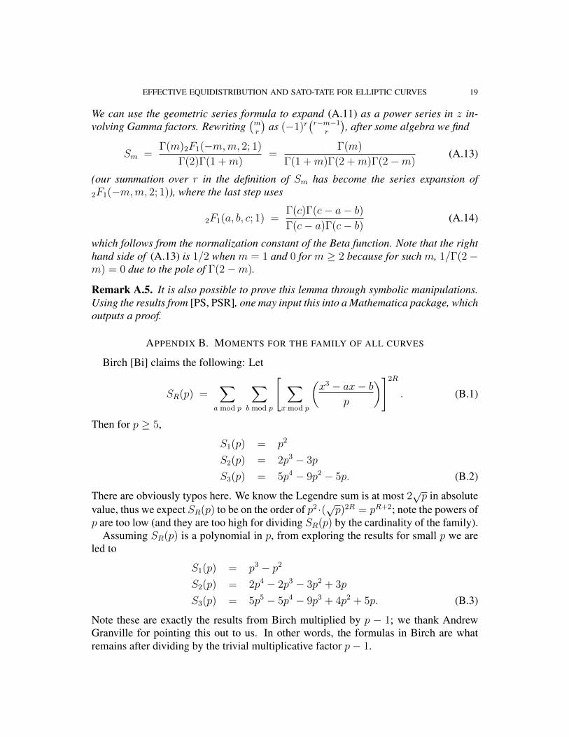
which follows from the normalization constant of the Beta function. Note that the righthand side of (A.13) is 1/2 when m = 1 and 0 for m ≥ 2 because for such m, 1/Γ(2−m) = 0 due to the pole of Γ(2−m).
Remark A.5. It is also possible to prove this lemma through symbolic manipulations.Using the results from [PS, PSR], one may input this into a Mathematica package, whichoutputs a proof.
APPENDIX B. MOMENTS FOR THE FAMILY OF ALL CURVES
Birch [Bi] claims the following: Let
SR(p) =∑
a mod p
∑
b mod p
[ ∑
x mod p
(x3 − ax− b
p
)]2R
. (B.1)
Then for p ≥ 5,
S1(p) = p2
S2(p) = 2p3 − 3p
S3(p) = 5p4 − 9p2 − 5p. (B.2)
There are obviously typos here. We know the Legendre sum is at most 2√p in absolute
value, thus we expect SR(p) to be on the order of p2 ⋅(√p)2R = pR+2; note the powers ofp are too low (and they are too high for dividing SR(p) by the cardinality of the family).
Assuming SR(p) is a polynomial in p, from exploring the results for small p we areled to
S1(p) = p3 − p2
S2(p) = 2p4 − 2p3 − 3p2 + 3p
S3(p) = 5p5 − 5p4 − 9p3 + 4p2 + 5p. (B.3)
Note these are exactly the results from Birch multiplied by p − 1; we thank AndrewGranville for pointing this out to us. In other words, the formulas in Birch are whatremains after dividing by the trivial multiplicative factor p− 1.
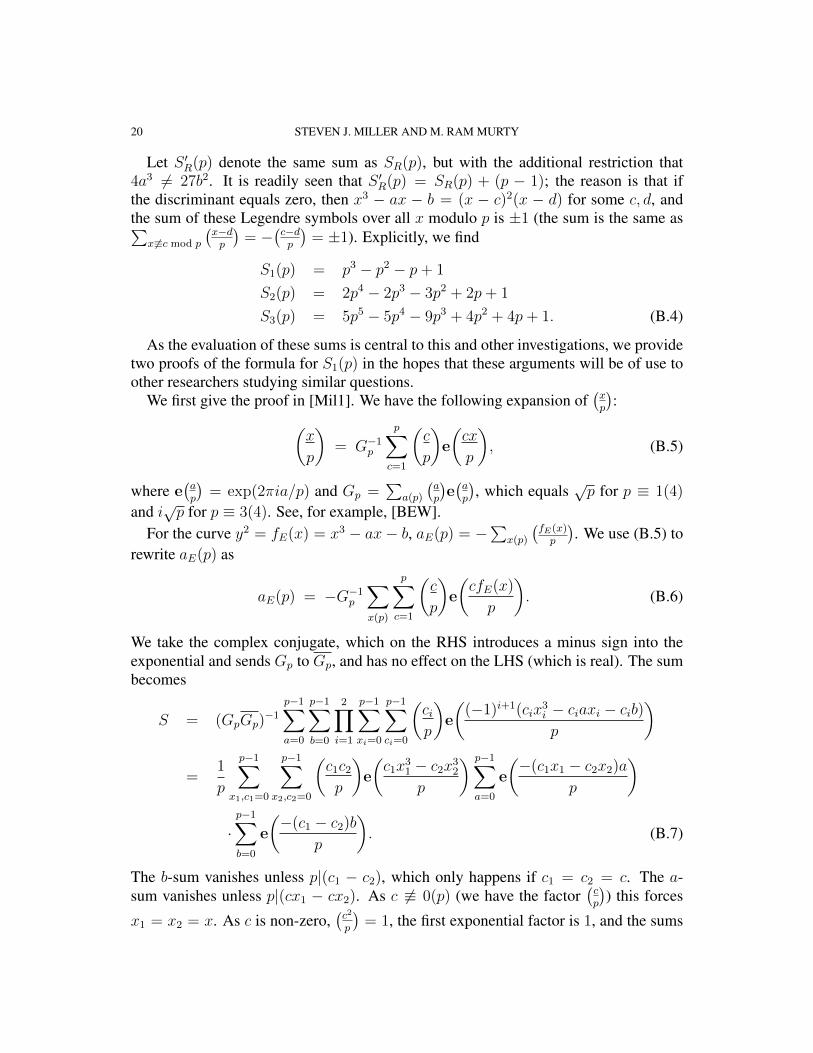
20 STEVEN J. MILLER AND M. RAM MURTY
Let S ′R(p) denote the same sum as SR(p), but with the additional restriction that
4a3 ∕= 27b2. It is readily seen that S ′R(p) = SR(p) + (p − 1); the reason is that if
the discriminant equals zero, then x3 − ax − b = (x − c)2(x − d) for some c, d, andthe sum of these Legendre symbols over all x modulo p is ±1 (the sum is the same as∑
x ∕≡c mod p
(x−dp
)= −(
c−dp
)= ±1). Explicitly, we find
S1(p) = p3 − p2 − p+ 1
S2(p) = 2p4 − 2p3 − 3p2 + 2p+ 1
S3(p) = 5p5 − 5p4 − 9p3 + 4p2 + 4p+ 1. (B.4)
As the evaluation of these sums is central to this and other investigations, we providetwo proofs of the formula for S1(p) in the hopes that these arguments will be of use toother researchers studying similar questions.
We first give the proof in [Mil1]. We have the following expansion of(xp
):
(x
p
)= G−1
p
p∑c=1
(c
p
)e
(cx
p
), (B.5)
where e(ap
)= exp(2¼ia/p) and Gp =
∑a(p)
(ap
)e(ap
), which equals
√p for p ≡ 1(4)
and i√p for p ≡ 3(4). See, for example, [BEW].
For the curve y2 = fE(x) = x3 − ax− b, aE(p) = −∑x(p)
(fE(x)
p
). We use (B.5) to
rewrite aE(p) as
aE(p) = −G−1p
∑
x(p)
p∑c=1
(c
p
)e
(cfE(x)
p
). (B.6)
We take the complex conjugate, which on the RHS introduces a minus sign into theexponential and sends Gp to Gp, and has no effect on the LHS (which is real). The sumbecomes
S = (GpGp)−1
p−1∑a=0
p−1∑
b=0
2∏i=1
p−1∑xi=0
p−1∑ci=0
(cip
)e
((−1)i+1(cix
3i − ciaxi − cib)
p
)
=1
p
p−1∑x1,c1=0
p−1∑x2,c2=0
(c1c2p
)e
(c1x
31 − c2x
32
p
) p−1∑a=0
e
(−(c1x1 − c2x2)a
p
)
⋅p−1∑
b=0
e
(−(c1 − c2)b
p
). (B.7)
The b-sum vanishes unless p∣(c1 − c2), which only happens if c1 = c2 = c. The a-sum vanishes unless p∣(cx1 − cx2). As c ∕≡ 0(p) (we have the factor
(cp
)) this forces
x1 = x2 = x. As c is non-zero,(c2
p
)= 1, the first exponential factor is 1, and the sums
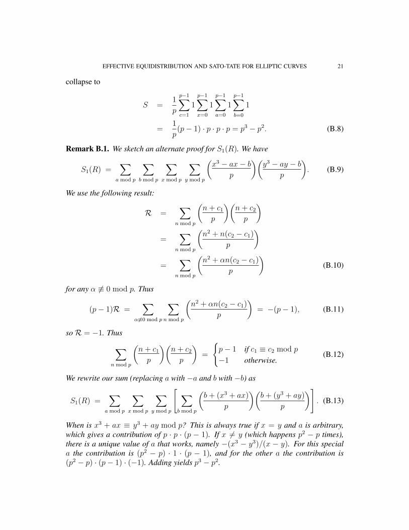
EFFECTIVE EQUIDISTRIBUTION AND SATO-TATE FOR ELLIPTIC CURVES 21
collapse to
S =1
p
p−1∑c=1
1
p−1∑x=0
1
p−1∑a=0
1
p−1∑
b=0
1
=1
p(p− 1) ⋅ p ⋅ p ⋅ p = p3 − p2. (B.8)
Remark B.1. We sketch an alternate proof for S1(R). We have
S1(R) =∑
a mod p
∑
b mod p
∑
x mod p
∑
y mod p
(x3 − ax− b
p
)(y3 − ay − b
p
). (B.9)
We use the following result:
ℛ =∑
n mod p
(n+ c1
p
)(n+ c2
p
)
=∑
n mod p
(n2 + n(c2 − c1)
p
)
=∑
n mod p
(n2 + ®n(c2 − c1)
p
)(B.10)
for any ® ∕≡ 0 mod p. Thus
(p− 1)ℛ =∑
® ∕≡0 mod p
∑
n mod p
(n2 + ®n(c2 − c1)
p
)= −(p− 1), (B.11)
so ℛ = −1. Thus
∑
n mod p
(n+ c1
p
)(n+ c2
p
)=
{p− 1 if c1 ≡ c2 mod p
−1 otherwise.(B.12)
We rewrite our sum (replacing a with −a and b with −b) as
S1(R) =∑
a mod p
∑
x mod p
∑
y mod p
[ ∑
b mod p
(b+ (x3 + ax)
p
)(b+ (y3 + ay)
p
)]. (B.13)
When is x3 + ax ≡ y3 + ay mod p? This is always true if x = y and a is arbitrary,which gives a contribution of p ⋅ p ⋅ (p − 1). If x ∕= y (which happens p2 − p times),there is a unique value of a that works, namely −(x3 − y3)/(x − y). For this speciala the contribution is (p2 − p) ⋅ 1 ⋅ (p − 1), and for the other a the contribution is(p2 − p) ⋅ (p− 1) ⋅ (−1). Adding yields p3 − p2.
22 STEVEN J. MILLER AND M. RAM MURTY
REFERENCES
[AL-RM] S. Arms, Á. Lozano-Robledo and S. J. Miller, Constructing one-parameter families of el-liptic curves over ℚ(T ) with moderate rank, Journal of Number Theory 123 (2007), no. 2,388–402.
[BZ] S. Baier and L. Zhao, The Sato-Tate conjecture on average for small angles, Transactionsof the AMS 361 (2009), no. 4, 1811–1832.
[BS] W. D. Banks and I. E. Shparlinski, Sato-Tate, cyclicity, and divisibility statistics on averagefor elliptic curves of small height, Israel J. Math. 173 (2009), 253–277.
[B-LGG] T. Barnet-Lamb, T. Gee and D. Geraghty, The Sato-Tate conjecture for Hilbert modularforms, preprint (2009). http://arxiv.org/abs/0912.1054.
[B-LGHT] T. Barnet-Lamb, D. Geraghty, M. Harris and R. Taylor, A familyof Calabi-Yau varieties and potential automorphy II., preprint (2009).http://www.math.harvard.edu/ rtaylor/cy2.pdf.
[BEW] B. Berndt, R. Evans and K. Williams, Gauss and Jacobi Sums, Canadian Mathematical So-ciety Series of Monographs and Advanced Texts, vol. 21, Wiley-Interscience Publications,John Wiley & Sons, Inc., New York, 1998.
[Bi] B. Birch, How the number of points of an elliptic curve over a fixed prime field varies, J.London Math. Soc. 43, 1968, 57− 60.
[BS-D1] B. Birch and H. Swinnerton-Dyer, Notes on elliptic curves. I, J. reine angew. Math. 212,1963, 7− 25.
[BS-D2] B. Birch and H. Swinnerton-Dyer, Notes on elliptic curves. II, J. reine angew. Math. 218,1965, 79− 108.
[BCDT] C. Breuil, B. Conrad, F. Diamond and R. Taylor, On the modularity of elliptic curves overQ: wild 3-adic exercises, J. Amer. Math. Soc. 14, no. 4, 2001, 843− 939.
[Bro] M. L. Brown, Heegner modules and elliptic curves, Lecture Notes In Mathematics, vol.1849, Springer-Verlag, 2004.
[CHT] L. Clozel, M. Harris and R. Taylor, Automorphy for some ℓ-adic lifts of automorphic mod ℓGalois representations, Publications Mathématiques de L’IHÉS 108 (2008), no. 1, 1–181.
[CW] J. Coates and A. Wiles, On the conjecture of Birch and Swinnerton-Dyer, Invent. Math. 39(1977), no. 3, 223–251.
[CDF] J. Brian Conrey, W. Duke and D. Farmer, The distribution of the eigenvalues of Heckeoperators, Acta Arithmetica 78 (1997), no. 4, 405–409.
[De] P. Deligne, La conjecture de Weil. II Inst. Hautes Études Sci. Publ. Math. 52, 1980, 137 −252.
[Deu] M. Deuring, Die Typen der Multiplikatorenringe elliptischer Funktionenkörper, Abh. Math.Sem. Hansischen Univ. 14 (1941), 197–272.
[Di] F. Diamond, On deformation rings and Hecke rings, Ann. Math. 144, 1996, 137− 166.[Fe1] S. Fermigier, Zéros des fonctions L de courbes elliptiques, Exper. Math. 1, 1992, 167−173.[Fe2] S. Fermigier, Étude expérimentale du rang de familles de courbes elliptiques sur ℚ, Exper.
Math. 5, 1996, 119− 130.[GKZ] B. H. Gross, W. Kohnen and D. B. Zagier, Heegner points and derivatives of L-series. II,
Mathematische Annalen 278 (1987), no. 1U4, 497–562.[GZ] B. H. Gross and D. B. Zagier, Heegner points and derivatives of L-series, Inventiones Math-
ematicae 84 (1986), no. 2, 225–320.[HS-BT] M. Harris, N. Shepherd-Barron and R. Taylor, A family of Calabi-Yau varieties and potential
automorphy, to appear in the Annals of Math.[He1] M. Hecke, Eine neue Art von Zetafunktionen und ihre Beziehungen zur Verteilung der
Primzahlen, I, Math. Z. 1 (1918), 357–376.
EFFECTIVE EQUIDISTRIBUTION AND SATO-TATE FOR ELLIPTIC CURVES 23
[He2] M. Hecke, Eine neue Art von Zetafunktionen und ihre Beziehungen zur Verteilung derPrimzahlen, II, Math. Z. 6 (1920), 11–51.
[Ka] N. Katz, Gauss Sums, Kloosterman Sums, and Monodromy Groups, Princeton UniversityPress, Princeton, NJ 1988.
[Kol1] V. A. Kolyvagin, The Mordell-Weil and Shafarevich-Tate groups for Weil elliptic curves,Izv. Akad. Nauk SSSR Ser. Mat. 52 (1988), no. 6, 1154–1180, 1327; translation in Math.USSR-Izv. 33 (1989), no. 3, 473–499
[Kol2] V. A. Kolyvagin, Finiteness of E(Q) and Shah(E,Q) for a subclass of Weil curves, Izv.Akad. Nauk SSSR Ser. Mat. 52 (1988), no. 3, 522–540, 670–671; translation in Math.USSR-Izv. 32 (1989), no. 3, 523–541.
[Mic] P. Michel, Rang moyen de familles de courbes elliptiques et lois de Sato-Tate, Monat. Math.120, 1995, 127− 136.
[Mil1] S. J. Miller, 1- and 2-Level Densities for Families of Elliptic Curves: Evidence for theUnderlying Group Symmetries, Princeton University, Ph. D. thesis, 2002.http://www.williams.edu/go/math/sjmiller/public html/math/thesis/thesis.html
[Mil2] S. J. Miller, Variation in the number of points on elliptic curves and applications to excessrank, C. R. Math. Rep. Acad. Sci. Canada 27 (2005), no. 4, 111–120.
[Mil3] S. J. Miller, Investigations of zeros near the central point of elliptic curve L-functions,Experimental Mathematics 15 (2006), no. 3, 257–279.
[Mil4] S. J. Miller, An identity for sums of polylogarithm functions, Integers: Electronic Journal OfCombinatorial Number Theory 8 (2008), #A15.
[MS] M. Ram Murty and K. Sinha, Effective equidistribution of eigenvalues of Hecke operators,Journal of Number Theory 129 (2009) 681–714.
[Na] K. Nagao, ℚ(t)-rank of elliptic curves and certain limit coming from the local points,Manuscr. Math. 92, 1997, 13− 32.
[PS] P. Paule and M. Schorn, A Mathematica Version of Zeilberger’s Algorithm for Proving Bi-nomial Coefficient Identities, J. Symbolic Computation 11 (1994), 1-25.
[PSR] P. Paule, M. Schorn and A. Riese, An Implementation Of Zeilberger’s Fast Algorithm,http://www.risc.uni-linz.ac.at/research/combinat/software/PauleSchorn/index.php
[RS] M. Rosen and J. Silverman, On the rank of an elliptic surface, Invent. Math. 133 (1998),43–67.
[Ru] K. Rubin, The one-variable main conjecture for elliptic curves with complex multiplication,L-functions and arithmetic (Durham, 1989), in London Math. Soc. Lecture Note Series 153,Cambridge Univ. Press, Cambridge, 1991, pages 353–371.
[Sar] P. Sarnak, Statistical properties of eigenvalues of the Hecke operators, in Analytic NumberTheory and Diophantine Problems (Stillwater, OK, 1984), Progr. Math. 70, Birkhäuser,Boston, 1987, 321–331.
[Sel] A. Selberg, On the estimation of Fourier Coefficients of Modular Forms, Proc. Amer. Math.Soc., Symposia in Pure Math. VIII: Theory of Numbers (Pasedena, 1963), 1–15.
[Ser] J.-P. Serre, Répartition Asymptotique des Valuers Propres de l’Operateur de Hecke Tp, J.Amer. Math. Soc. 10 (1997), no. 1, 75–102.
[Sh1] I. E. Shparlinski, On the Lang-Trotter and Sato-Tate Conjectures on Average for Some Fam-ilies of Elliptic Curves, preprint.
[Sh2] I. E. Shparlinski, On the Sato-Tate Conjecture on Average for Some Families of EllipticCurves, preprint.
24 STEVEN J. MILLER AND M. RAM MURTY
[Sil1] J. Silverman, The Arithmetic of Elliptic Curves, Graduate Texts in Mathematics 106,Springer-Verlag, Berlin - New York, 1986.
[Sil2] J. Silverman, Advanced Topics in the Arithmetic of Elliptic Curves, Graduate Texts in Math-ematics 151, Springer-Verlag, Berlin - New York, 1994.
[ST] J. Silverman and J. Tate, Rational Points on Elliptic Curves, Springer-Verlag, New York,1992.
[Ta] J. T. Tate, Algebraic cycles and poles of zeta-functions, in Arithmetical Algebraic geometry(Proc. Purdue Conf. 1963), O. F. G. Schilling (ed.), Harper & Row, 1965, pp. 93–110.
[Tay] R. Taylor, Automorphy for some ℓ-adic lifts of automorphic mod ℓ Galois representations.II, Publications Mathématiques de L’IHÉS 108 (2008), no. 1, 183–239.
[TW] R. Taylor and A. Wiles, Ring-theoretic properties of certain Hecke algebras, Ann. Math.141, 1995, 553− 572.
[Ward] K. J. Ward, Series Sums of Binomial Coefficients, webpage:http://www.trans4mind.com/personal development/mathematics/series/summingBinomialCoefficients.htm
[Wa] L. Washington, Class numbers of the simplest cubic fields, Math. Comp. 48, number 177,1987, 371− 384.
[Wi] Wikipedia, Chebyshev Polynomials, June 21, 2009.http://en.wikipedia.org/wiki/Chebyshev polynomials.
E-mail address: [email protected]
DEPARTMENT OF MATHEMATICS AND STATISTICS, WILLIAMS COLLEGE, WILLIAMSTOWN, MA01267
E-mail address: [email protected]
DEPARTMENT OF MATHEMATICS, QUEEN’S UNIVERSITY, KINGSTON, ONTARIO, K7L 3N6, CANADA


![Arakelov geometry, heights, equidistribution, and the ... › pdf › 1904.05630.pdfarXiv:1904.05630v2 [math.NT] 4 Nov 2019 Arakelov geometry, heights, equidistribution, and the Bogomolov](https://img.pdfslide.net/doc/110x75/5ed8366b0fa3e705ec0e0b81/arakelov-geometry-heights-equidistribution-and-the-a-pdf-a-190405630pdf.jpg)