Embed Size (px)
Citation preview
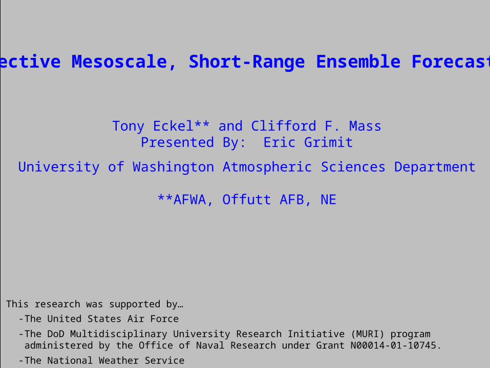
Effective Mesoscale, Short-Range Ensemble Forecasting
Tony Eckel** and Clifford F. MassPresented By: Eric Grimit
University of Washington Atmospheric Sciences Department
**AFWA, Offutt AFB, NE
This research was supported by…
- The United States Air Force
- The DoD Multidisciplinary University Research Initiative (MURI) program administered by the Office of Naval Research under Grant N00014-01-10745.
- The National Weather Service
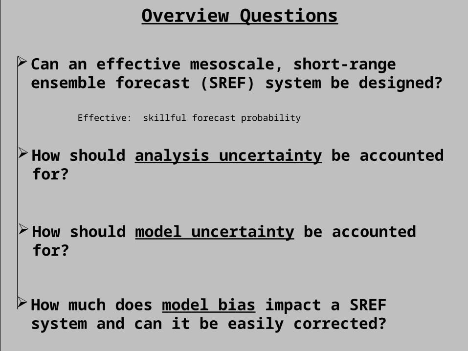
Overview Questions
Can an effective mesoscale, short-range ensemble forecast (SREF) system be designed?
Effective: skillful forecast probability
How should analysis uncertainty be accounted for?
How much does model bias impact a SREF system and can it be easily corrected?
How should model uncertainty be accounted for?
FP = 93%
Event Threshold
FP = ORF = 72%
Fre
qu
en
cy
Initial State
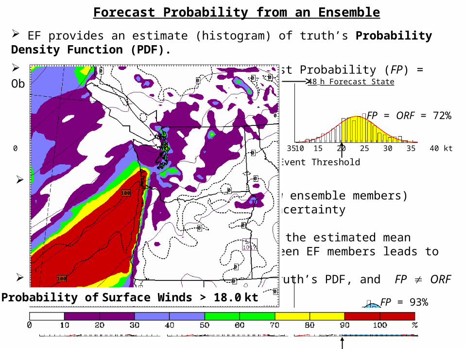
Forecast Probability from an Ensemble
EF provides an estimate (histogram) of truth’s Probability Density Function (PDF).
In a large, ideal EF system, Forecast Probability (FP) = Observed Relative Frequency (ORF)
24 h Forecast State 48 h Forecast State
True
0 5 10 15 20 25 30 35 40 kt0 5 10 15 20 25 30 350 5 10 15 20 25 30 35Surface Wind Speed (kt)
Fre
qu
ency
Fre
qu
en
cy
In practice, things go awry from…• Undersampling of the PDF (too few ensemble members)• Poor representation of initial uncertainty• Model deficiencies
-- Model bias causes a shift in the estimated mean-- Sharing of model errors between EF members leads to reduced variance
EF’s estimated PDF does not match truth’s PDF, and FP ORF
Fre
qu
ency
Probability of Surface Winds > 18.0 kt
0
0
0
0
0
0
0
0
0
0
0
0
0
0
100
100
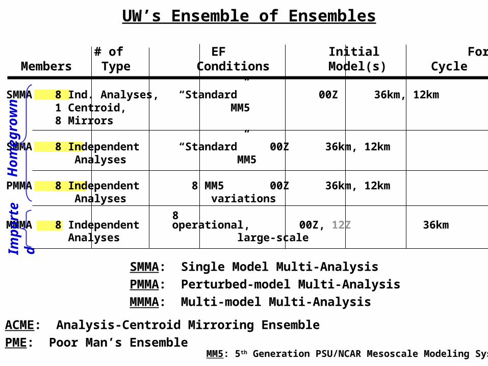
UW’s Ensemble of Ensembles
# of EF Initial Forecast Forecast Name Members Type Conditions Model(s) Cycle Domain
ACME 17 SMMA 8 Ind. Analyses, “Standard” 00Z 36km, 12km1 Centroid, MM58 Mirrors
UWME 8 SMMA 8 Independent “Standard” 00Z 36km, 12km Analyses MM5
UWME+ 8 PMMA 8 Independent 8 MM5 00Z 36km, 12km Analyses variations
8 PME 8 MMMA 8 Independent operational, 00Z, 12Z 36km
Analyses large-scale
Hom
egro
wn
Impo
rted
ACME: Analysis-Centroid Mirroring Ensemble
PME: Poor Man’s Ensemble MM5: 5th Generation PSU/NCAR Mesoscale Modeling System
SMMA: Single Model Multi-Analysis
PMMA: Perturbed-model Multi-Analysis
MMMA: Multi-model Multi-Analysis
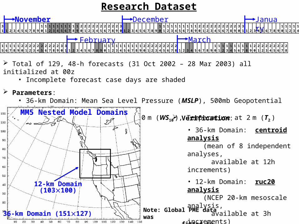
Total of 129, 48-h forecasts (31 Oct 2002 – 28 Mar 2003) all initialized at 00z• Incomplete forecast case days are shaded
Parameters:• 36-km Domain: Mean Sea Level Pressure (MSLP), 500mb Geopotential Height (Z500 )• 12-km Domain: Wind Speed at 10 m (WS10 ), Temperature at 2 m (T2 )
Research Dataset
Verification:
• 36-km Domain: centroid analysis (mean of 8 independent analyses, available at 12 h increments)
• 12-km Domain: ruc20 analysis (NCEP 20-km mesoscale analysis, available at 3 h increments)
November December January
February March
3 1 1 1 1 1 1 1 1 1 1 2 2 2 2 2 2 2 2 2 2 3 1 1 1 1 1 1 1 1 1 1 2 2 2 2 2 2 2 2 2 2 3 3 1 1 1 1 11 1 2 3 4 5 6 7 8 9 0 1 2 3 4 5 6 7 8 9 0 1 2 3 4 5 6 7 8 9 0 1 2 3 4 5 6 7 8 9 0 1 2 3 4 5 6 7 8 9 0 1 2 3 4 5 6 7 8 9 0 1 1 2 3 4 5 6 7 8 9 0 1 2 3 4
1 1 1 1 1 2 2 2 2 2 2 2 2 2 2 3 3 1 1 1 1 1 1 1 1 1 1 2 2 2 2 2 2 2 2 2 1 1 1 1 1 1 1 1 1 1 2 2 2 2 2 2 2 2 2 25 6 7 8 9 0 1 2 3 4 5 6 7 8 9 0 1 1 2 3 4 5 6 7 8 9 0 1 2 3 4 5 6 7 8 9 0 1 2 3 4 5 6 7 8 1 2 3 4 5 6 7 8 9 0 1 2 3 4 5 6 7 8 9 0 1 2 3 4 5 6 7 8 9
36-km Domain (151127)
12-km Domain(103100)
Note: Global PME data was fitted to the 36-km domain
MM5 Nested Model Domains
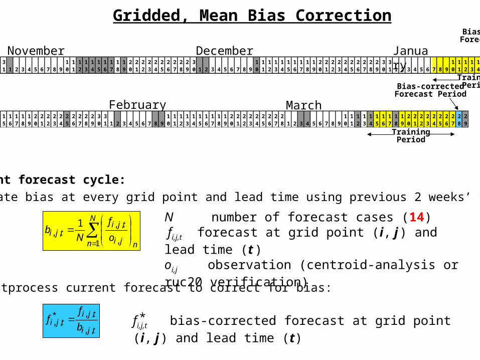
TrainingPeriod
Bias-correctedForecast Period
TrainingPeriod
Bias-correctedForecast Period
Gridded, Mean Bias Correction
N
n nji
tjitji o
f
Nb
1 ,
,,,,
1 N number of forecast cases (14) fi,j,t forecast at grid point (i, j ) and lead time (t )oi,j observation (centroid-analysis or ruc20 verification)
For the current forecast cycle:
1) Calculate bias at every grid point and lead time using previous 2 weeks’ forecasts
2) Postprocess current forecast to correct for bias:
tji
tjitji b
ff
,,
,,*,, fi,j,t bias-corrected forecast at grid point (i, j ) and lead time (t)*
November December January
February March
3 1 1 1 1 1 1 1 1 1 1 2 2 2 2 2 2 2 2 2 2 3 1 1 1 1 1 1 1 1 1 1 2 2 2 2 2 2 2 2 2 2 3 3 1 1 1 1 11 1 2 3 4 5 6 7 8 9 0 1 2 3 4 5 6 7 8 9 0 1 2 3 4 5 6 7 8 9 0 1 2 3 4 5 6 7 8 9 0 1 2 3 4 5 6 7 8 9 0 1 2 3 4 5 6 7 8 9 0 1 1 2 3 4 5 6 7 8 9 0 1 2 3 4
1 1 1 1 1 2 2 2 2 2 2 2 2 2 2 3 3 1 1 1 1 1 1 1 1 1 1 2 2 2 2 2 2 2 2 2 1 1 1 1 1 1 1 1 1 1 2 2 2 2 2 2 2 2 2 25 6 7 8 9 0 1 2 3 4 5 6 7 8 9 0 1 1 2 3 4 5 6 7 8 9 0 1 2 3 4 5 6 7 8 9 0 1 2 3 4 5 6 7 8 1 2 3 4 5 6 7 8 9 0 1 2 3 4 5 6 7 8 9 0 1 2 3 4 5 6 7 8 9
Ave
rage
RM
SE
(C
)an
d
(sh
aded
) A
vera
ge B
ias
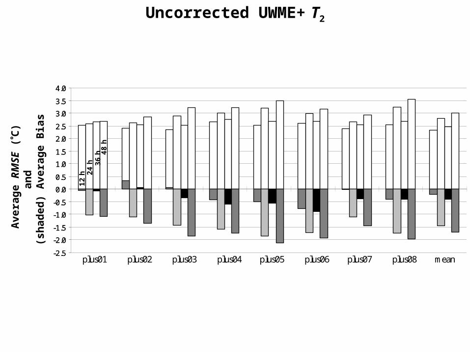
Uncorrected UWME+ T2
-2.5
-2.0
-1.5
-1.0
-0.5
0.0
0.5
1.0
1.5
2.0
2.5
3.0
3.5
4.0
Ave
rag
e R
MS
E a
nd
Bia
s (C
)
plus01 plus02 plus03 plus04 plus05 plus06 plus07 plus08 mean -2.5
-2.0
-1.5
-1.0
-0.5
0.0
0.5
1.0
1.5
2.0
2.5
3.0
3.5
4.0
Ave
rag
e R
MS
E a
nd
Bia
s (m
b)
12 h
24 h 36
h 48 h
-2.5
-2.0
-1.5
-1.0
-0.5
0.0
0.5
1.0
1.5
2.0
2.5
3.0
3.5
4.0
Ave
rag
e R
MS
E a
nd
Bia
s (m
b)
plus01 plus02 plus03 plus04 plus05 plus06 plus07 plus08 mean -2.5
-2.0
-1.5
-1.0
-0.5
0.0
0.5
1.0
1.5
2.0
2.5
3.0
3.5
4.0
Ave
rag
e R
MS
E a
nd
Bia
s (m
b)
Ave
rage
RM
SE
(C
)an
d
(sh
aded
) A
vera
ge B
ias
Bias-Corrected UWME+ T2
12 h
24 h 36
h 48 h
-2.5
-2.0
-1.5
-1.0
-0.5
0.0
0.5
1.0
1.5
2.0
2.5
3.0
3.5
4.0
plus01 plus02 plus03 plus04 plus05 plus06 plus07 plus08 mean -2.5
-2.0
-1.5
-1.0
-0.5
0.0
0.5
1.0
1.5
2.0
2.5
3.0
3.5
4.0
MultimodelVs.
Perturbed Model
PMEVs.
UWME+
36-km
Domain
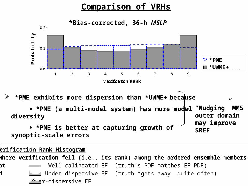
*PME exhibits more dispersion than *UWME+ because
*PME (a multi-model system) has more model diversity
*PME is better at capturing growth of synoptic-scale errors
1 2 3 4 5 6 7 8 936h PME0.0
0.1
0.2
0.3
0.4
Verification Rank
36h PME
36h ACMEcore+
*PME*UWME+
Pro
bab
ilit
y
Verification Rank Histogram
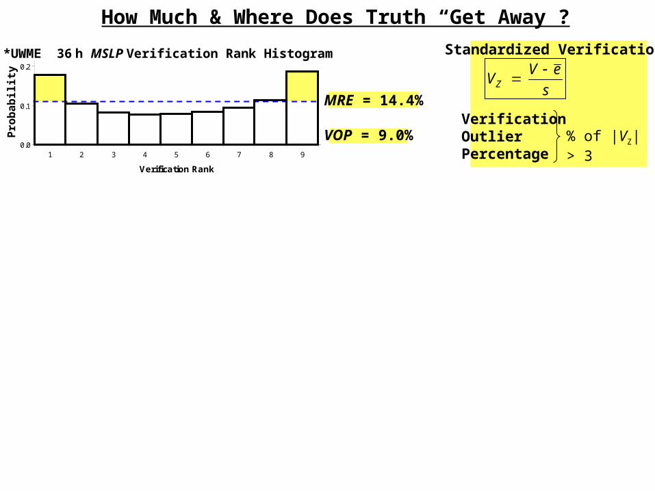
Record of where verification fell (i.e., its rank) among the ordered ensemble members:
Flat Well calibrated EF (truth’s PDF matches EF PDF)
U’d Under-dispersive EF (truth “gets away” quite often)
Humped Over-dispersive EF
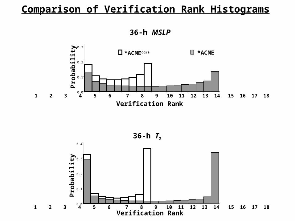
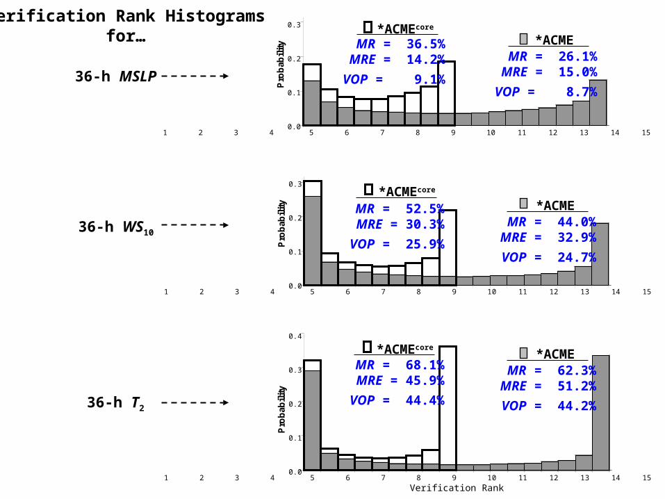
*Bias-corrected, 36-h MSLP
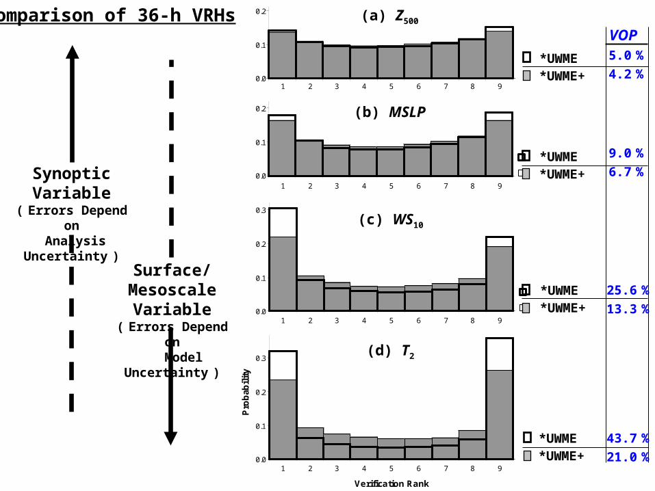
Comparison of VRHs
“Nudging” MM5 outer domain may improve SREF
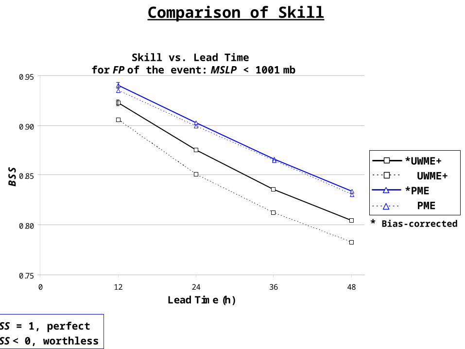
Skill vs. Lead Time for FP of the event: MSLP < 1001 mb
BSS = 1, perfect
BSS < 0, worthless
Comparison of Skill
-0.1
0.0
0.1
0.2
0.3
0.4
0.5
0.6
00 03 06 09 12 15 18 21 24 27 30 33 36 39 42 45 48
*ACMEcoreACMEcore*ACMEcore+ACMEcore+Uncertainty
*UWME+
UWME+
*PME
PME
0.75
0.80
0.85
0.90
0.95
0 12 24 36 48
Lead Time (h)
BSS
0.75
0 12 24 36 48
*PME
PME
0.75
0 12 24 36 48
* Bias-corrected

Value ofModel Diversity
For a Mesoscale SREF
UWMEVs.
UWME+
12-km
Domain
s
eVVZ
Standardized Verification
VerificationOutlierPercentage
% of |VZ| > 3
Pro
bab
ilit
y
*UWME 36 h MSLP Verification Rank Histogram
MRE = 14.4%
VOP = 9.0%
How Much & Where Does Truth “Get Away”?
1 2 3 4 5 6 7 8 936h ACMEcore0.0
0.1
0.2
0.3
0.4
Pro
bab
ilit
y
Verification Rank
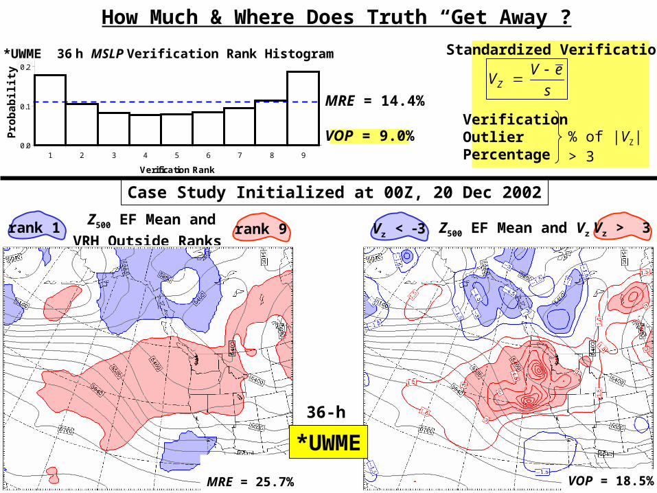
Case Study Initialized at 00Z, 20 Dec 2002
rank 9 Vz < 3 Vz > 3Z500 EF Mean and Vzrank 1Z500 EF Mean and
VRH Outside Ranks
MRE = 25.7% VOP = 18.5%
*UWME
36-h
s
eVVZ
Standardized Verification
VerificationOutlierPercentage
% of |VZ| > 31 2 3 4 5 6 7 8 9
36h ACMEcore0.0
0.1
0.2
0.3
0.4
Pro
bab
ilit
y
Verification Rank
Pro
bab
ilit
y
*UWME 36 h MSLP Verification Rank Histogram
MRE = 14.4%
VOP = 9.0%
How Much & Where Does Truth “Get Away”?
1 2 3 4 5 6 7 8 936h *ACMEcore0.0
0.1
0.2
0.3
0.4
1 2 3 4 5 6 7 8 936h *ACMEcore0.0
0.1
0.2
0.3
0.4
36h *ACMEcore
36h *ACMEcore+
1 2 3 4 5 6 7 8 936h *ACMEcore0.0
0.1
0.2
0.3
0.4
36h *ACMEcore
36h *ACMEcore+
1 2 3 4 5 6 7 8 936h *ACMEcore0.0
0.1
0.2
0.3
0.4
Pro
bab
ilit
y
Verification Rank
(d) T2
(c) WS10
(b) MSLP
1 2 3 4 5 6 7 8 936h ACMEcore0.0
0.1
0.2
0.3
0.4
1 2 3 4 5 6 7 8 936h ACMEcore0.0
0.1
0.2
0.3
0.4
Verification Rank
(a) Z500
1 2 3 4 5 6 7 8 936h ACMEcore0.0
0.1
0.2
0.3
0.4
Verification Rank
1 2 3 4 5 6 7 8 936h ACMEcore0.0
0.1
0.2
0.3
0.4
*UWME*UWME+
VOP 5.0 %
4.2 %
9.0 %
6.7 %
25.6 %
13.3 %
43.7 %
21.0 %
Surface/Mesoscale Variable
( Errors Depend on Model Uncertainty )
SynopticVariable
( Errors Depend on Analysis Uncertainty )
Comparison of 36-h VRHs
*UWME*UWME+
*UWME*UWME+
*UWME*UWME+
-0.1
0.0
0.1
0.2
0.3
0.4
0.5
0.6
00 03 06 09 12 15 18 21 24 27 30 33 36 39 42 45 48
*ACMEcoreACMEcore*ACMEcore+ACMEcore+Uncertainty
*UWME
UWME
*UWME+
UWME+
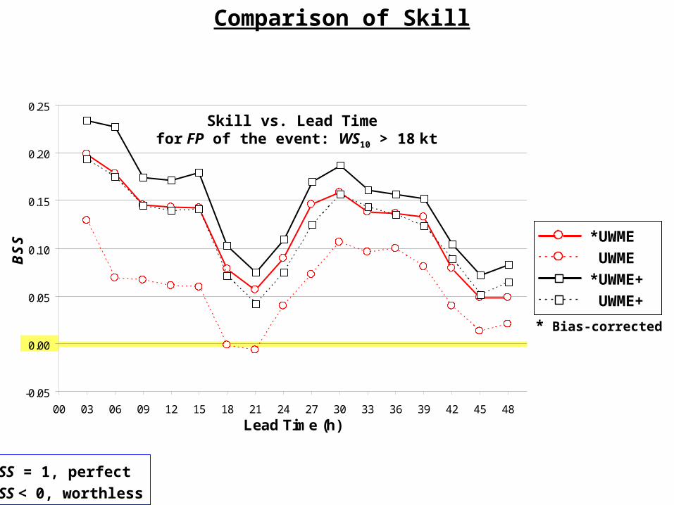
Comparison of Skill
Skill vs. Lead Time for FP of the event: WS10 > 18 kt
-0.05
0.00
0.05
0.10
0.15
0.20
0.25
00 03 06 09 12 15 18 21 24 27 30 33 36 39 42 45 48
Lead Time (h)
BSS
-0.05
00 03 06 09 12 15 18 21 24 27 30 33 36 39 42 45 48
BSS = 1, perfect
BSS < 0, worthless
* Bias-corrected
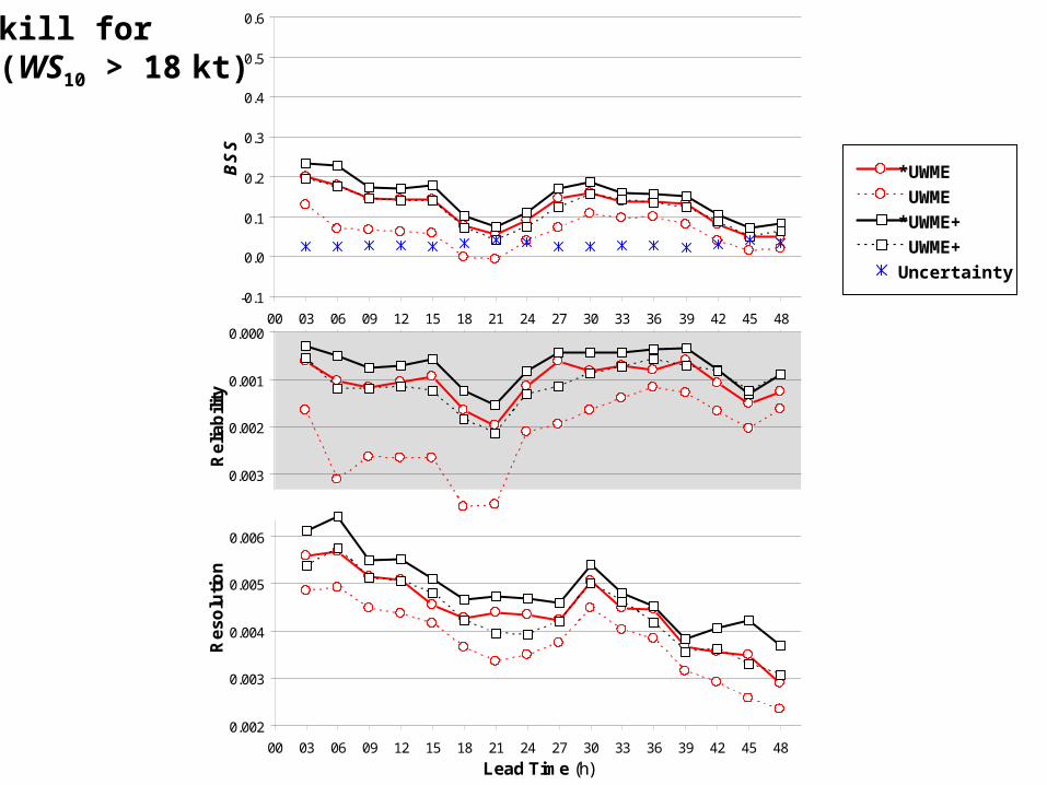
0.000
0.001
0.002
0.003
0.004
Re
liab
ility
0.002
0.003
0.004
0.005
0.006
0.007
00 03 06 09 12 15 18 21 24 27 30 33 36 39 42 45 48
Lead Time (h)
Re
so
luti
on
-0.1
0.0
0.1
0.2
0.3
0.4
0.5
0.6
00 03 06 09 12 15 18 21 24 27 30 33 36 39 42 45 48
BSS
-0.1
0.0
0.1
0.2
0.3
0.4
0.5
0.6
00 03 06 09 12 15 18 21 24 27 30 33 36 39 42 45 48
*ACMEcoreACMEcore*ACMEcore+ACMEcore+Uncertainty
*UWME
UWME
*UWME+
UWME+
Uncertainty
Skill forP(WS10 > 18 kt)
Conclusions
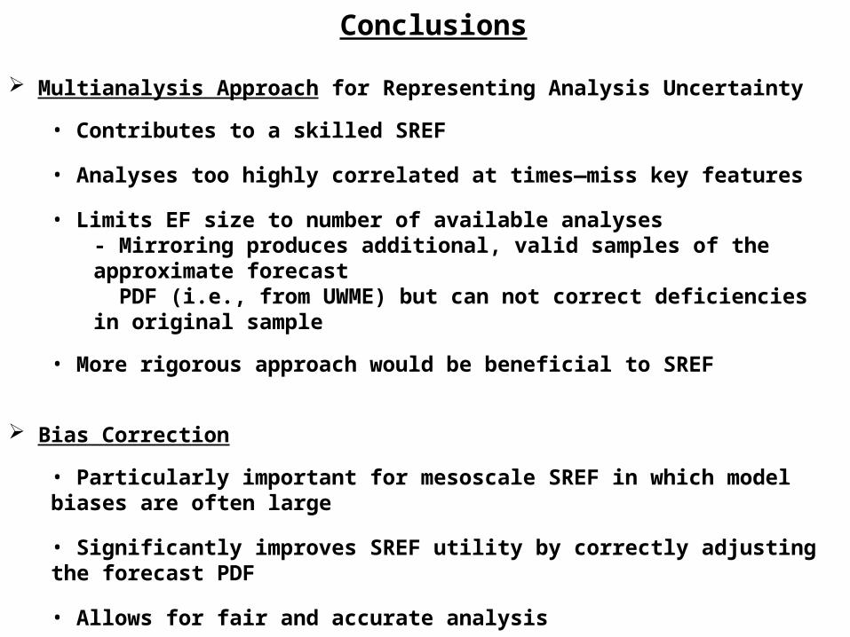
Bias Correction
• Particularly important for mesoscale SREF in which model biases are often large
• Significantly improves SREF utility by correctly adjusting the forecast PDF
• Allows for fair and accurate analysis
Multianalysis Approach for Representing Analysis Uncertainty
• Contributes to a skilled SREF
• Analyses too highly correlated at times—miss key features
• Limits EF size to number of available analyses- Mirroring produces additional, valid samples of the approximate forecast PDF (i.e., from UWME) but can not correct deficiencies in original sample
• More rigorous approach would be beneficial to SREF
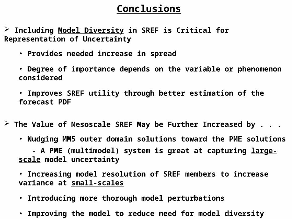
Including Model Diversity in SREF is Critical for Representation of Uncertainty
• Provides needed increase in spread
• Degree of importance depends on the variable or phenomenon considered
• Improves SREF utility through better estimation of the forecast PDF
Conclusions
The Value of Mesoscale SREF May be Further Increased by . . .
• Nudging MM5 outer domain solutions toward the PME solutions
- A PME (multimodel) system is great at capturing large-scale model uncertainty
• Increasing model resolution of SREF members to increase variance at small-scales
• Introducing more thorough model perturbations
• Improving the model to reduce need for model diversity

The End

Backup Slides
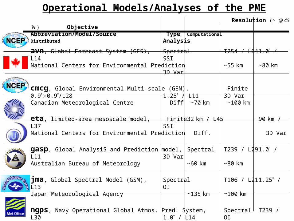
Resolution (~ @ 45 N ) ObjectiveAbbreviation/Model/Source Type Computational Distributed Analysis
avn, Global Forecast System (GFS), Spectral T254 / L64 1.0 / L14 SSINational Centers for Environmental Prediction ~55 km ~80 km 3D Var cmcg, Global Environmental Multi-scale (GEM), Finite 0.90.9/L28 1.25 / L11 3D VarCanadian Meteorological Centre Diff ~70 km ~100 km eta, limited-area mesoscale model, Finite 32 km / L45 90 km / L37 SSINational Centers for Environmental Prediction Diff. 3D Var gasp, Global AnalysiS and Prediction model, Spectral T239 / L29 1.0 / L11 3D VarAustralian Bureau of Meteorology ~60 km ~80 km
jma, Global Spectral Model (GSM), Spectral T106 / L21 1.25 / L13 OIJapan Meteorological Agency ~135 km ~100 km ngps, Navy Operational Global Atmos. Pred. System, Spectral T239 / L30 1.0 / L14 OIFleet Numerical Meteorological & Oceanographic Cntr. ~60 km ~80 km
tcwb, Global Forecast System, Spectral T79 / L18 1.0 / L11 OITaiwan Central Weather Bureau ~180 km ~80 km ukmo, Unified Model, Finite 5/65/9/L30 same / L12 3D VarUnited Kingdom Meteorological Office Diff. ~60 km
Operational Models/Analyses of the PME
Perturbed surface boundary parameters according to their suspected uncertainty
Assumed differences between model physics options approximate model error
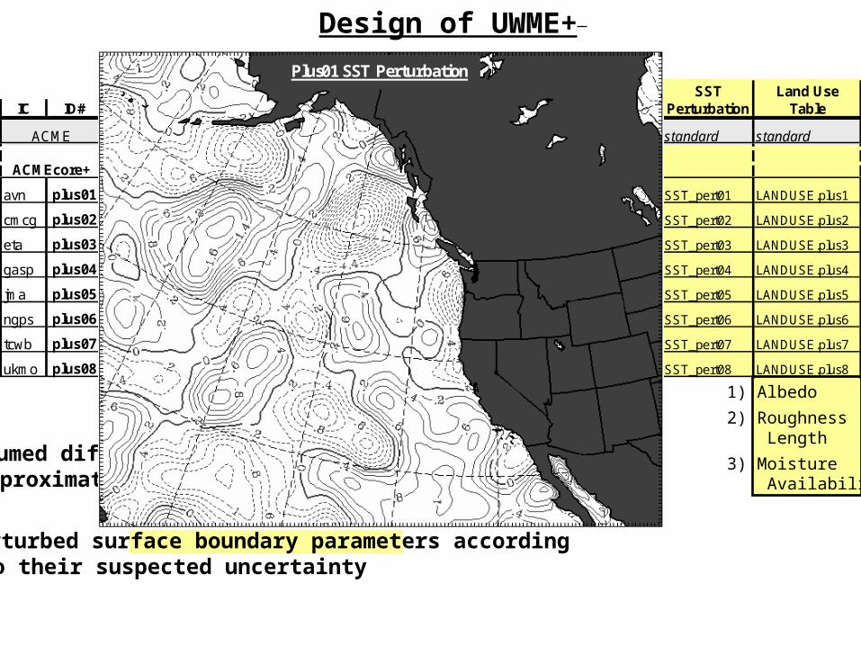
Design of UWME+
vertical Cloud 36-km 12-km shlw. SST Land UseIC ID# Soil diffusion Microphysics Domain Domain cumls. Radiation Perturbation Table
MRF 5-Layer Y Simple Ice Kain-Fritsch Kain-Fritsch N cloud standard standard
avn plus01 MRF LSM Y Simple Ice Kain-Fritsch Kain-Fritsch Y RRTM SST_pert01 LANDUSE.plus1
cmcg plus02 MRF 5-Layer Y Reisner II Grell Grell N cloud SST_pert02 LANDUSE.plus2
eta plus03 Eta 5-Layer N Goddard Betts-Miller Grell Y RRTM SST_pert03 LANDUSE.plus3
gasp plus04 MRF LSM Y Shultz Betts-Miller Kain-Fritsch N RRTM SST_pert04 LANDUSE.plus4
jma plus05 Eta LSM N Reisner II Kain-Fritsch Kain-Fritsch Y cloud SST_pert05 LANDUSE.plus5
ngps plus06 Blackadar 5-Layer Y Shultz Grell Grell N RRTM SST_pert06 LANDUSE.plus6
tcwb plus07 Blackadar 5-Layer Y Goddard Betts-Miller Grell Y cloud SST_pert07 LANDUSE.plus7
ukmo plus08 Eta LSM N Reisner I Kain-Fritsch Kain-Fritsch N cloud SST_pert08 LANDUSE.plus8Perturbations to
moisture availability,
albedo, and
roughness length
ACMEcore+
CumulusPBL
ACME
1) Albedo
2) Roughness Length
3) Moisture Availability
Plus01 SST PerturbationPlus01 SST Perturbation
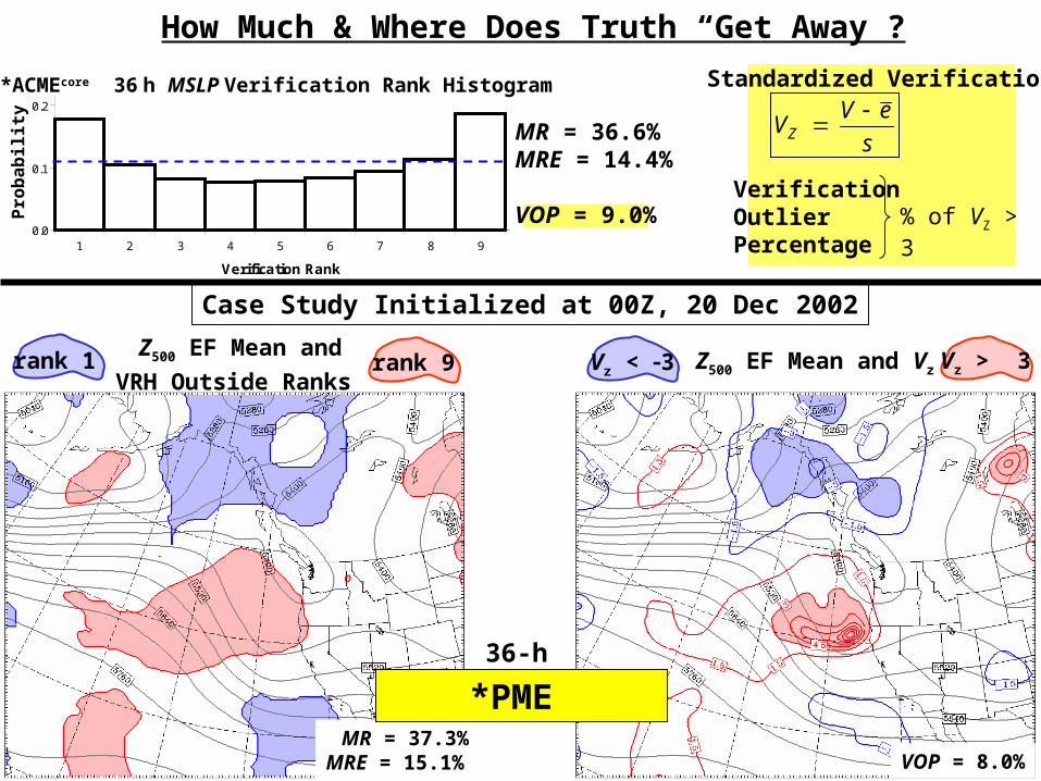
VOP = 8.0% MR = 37.3%MRE = 15.1%
*PME
Case Study Initialized at 00Z, 20 Dec 2002
rank 9 Vz < 3 Vz > 3Z500 EF Mean and Vzrank 1Z500 EF Mean and
VRH Outside Ranks
s
eVVZ
Standardized Verification
VerificationOutlierPercentage
% of VZ > 31 2 3 4 5 6 7 8 9
36h ACMEcore0.0
0.1
0.2
0.3
0.4
Pro
bab
ilit
y
Verification Rank
Pro
bab
ilit
y
*ACMEcore 36 h MSLP Verification Rank Histogram
MR = 36.6%MRE = 14.4%
VOP = 9.0%
36-h
How Much & Where Does Truth “Get Away”?
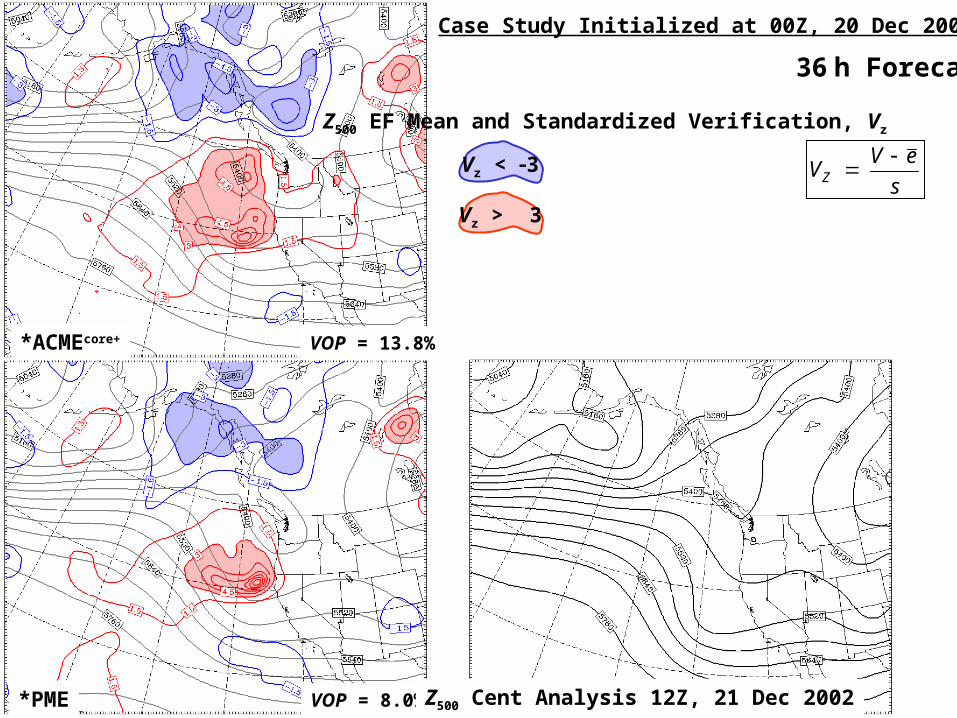
VOP = 13.8%
VOP = 8.0%
*ACMEcore+
*PME Z500 Cent Analysis 12Z, 21 Dec 2002
Case Study Initialized at 00Z, 20 Dec 2002
36 h Forecast
Z500 EF Mean and Standardized Verification, Vz
Vz < 3
Vz > 3s
eVVZ
-0.1
0.0
0.1
0.2
0.3
0.4
0.5
0.6
00 03 06 09 12 15 18 21 24 27 30 33 36 39 42 45 48
BSS
-0.1
0.0
0.1
0.2
0.3
0.4
0.5
0.6
00 03 06 09 12 15 18 21 24 27 30 33 36 39 42 45 48
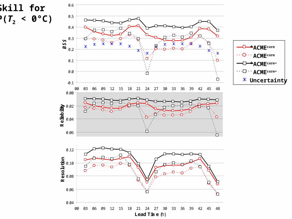
*ACMEcoreACMEcore*ACMEcore+ACMEcore+Uncertainty
0.00
0.02
0.04
0.06
Re
liab
ility
0.04
0.06
0.08
0.10
0.12
0.14
00 03 06 09 12 15 18 21 24 27 30 33 36 39 42 45 48
Lead Time (h)
Re
so
luti
on
*ACMEcore
ACMEcore
*ACMEcore+
ACMEcore+
Uncertainty
Skill forP(T2 < 0°C)
0.0
0.5
1.0
1.5
2.0
2.5
3.0
3.5
4.0
4.5
5.0
0 12 24 36 48
Lead Time (h)
EF
Sp
rea
d
or
M
SE
of
EF
Me
an
0.0
0.5
1.0
1.5
2.0
2.5
3.0
3.5
4.0
4.5
0 12 24 36 48
Lead Time (h)
EF
Sp
rea
d
or
M
SE
of
EF
Me
an
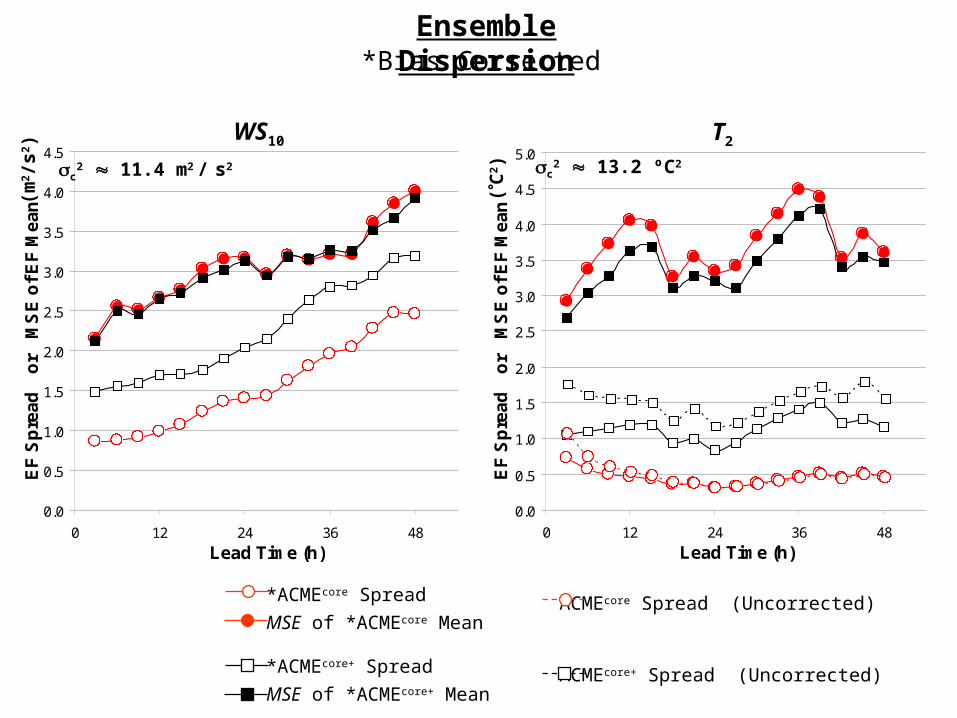
(m2 /
s2 )
(C2 )
WS10 T2
*ACMEcore Spread
MSE of *ACMEcore Mean
*ACMEcore+ Spread
MSE of *ACMEcore+ Mean
c2 11.4 m2 / s2 c
2 13.2 ºC2
Ensemble Dispersion*Bias Corrected
0.0
0 12 24 36 48
ACMEcore Spread (Uncorrected)
ACMEcore+ Spread (Uncorrected)
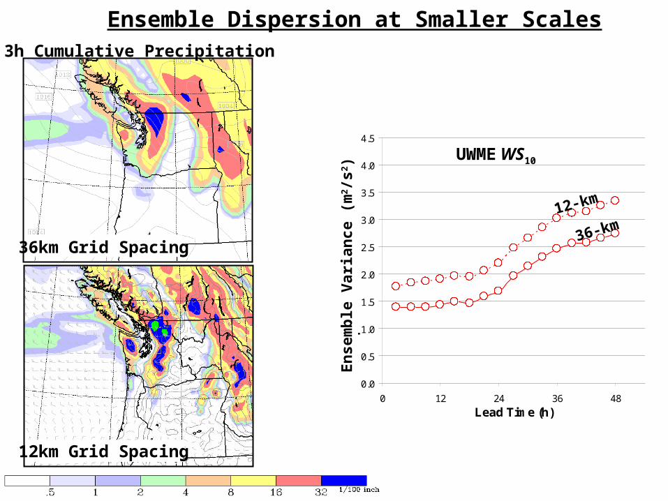
Ensemble Dispersion at Smaller Scales
0.0
0.5
1.0
1.5
2.0
2.5
3.0
3.5
4.0
4.5
0 12 24 36 48
Lead Time (h)
EF
Sp
rea
d
or
M
SE
of
EF
Me
an
En
sem
ble
Var
ian
ce (
m2 /
s2 )
UWME WS10
36-km12-km
36 km Grid Spacing
12 km Grid Spacing
3 h Cumulative Precipitation
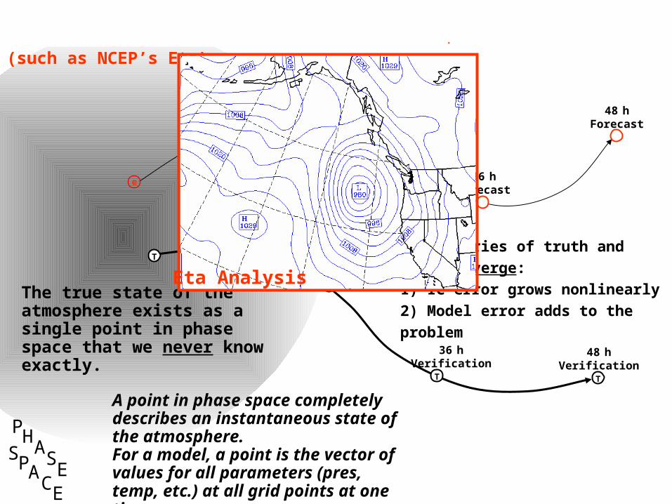
An analysis is just one possible initial condition (IC) used to run a numerical model (such as NCEP’s Eta).
T
The true state of the atmosphere exists as a single point in phase space that we never know exactly.
A point in phase space completely describes an instantaneous state of the atmosphere.For a model, a point is the vector of values for all parameters (pres, temp, etc.) at all grid points at one time.
e
Trajectories of truth and model diverge:
1) IC error grows nonlinearly
2) Model error adds to the problem
PHA
SE
SPACE
12 hForecast
36 hForecast
24 hForecast
48 hForecast
T
48 hVerification
T
36 hVerification
T
24 hVerification
T
12 hVerification
Eta Analysis
e
a
uc
j
tg
n
2 1 0 1 2 34
2
0
2
4
6
7
-2.96564
Core ,i 2
Cent ,1 2
32.5 ,Core ,i 1 Cent ,1 1
T
T
Analysis Region
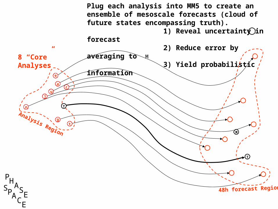
8 “Core” Analyses
Plug each analysis into MM5 to create an ensemble of mesoscale forecasts (cloud of future states encompassing truth).
1) Reveal uncertainty in forecast 2) Reduce error by averaging to M 3) Yield probabilistic information
M
48h forecast Region
PHA
SE
SPACE
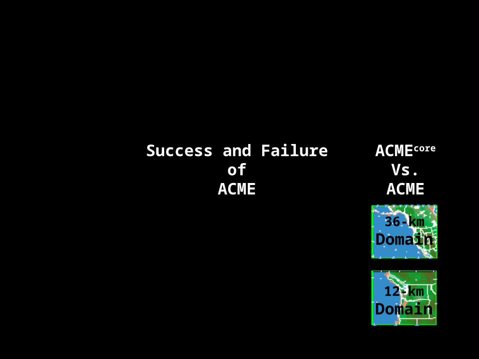
Success and Failureof
ACME
ACMEcore
Vs.ACME
36-km
Domain
12-km
Domain
cmcg*
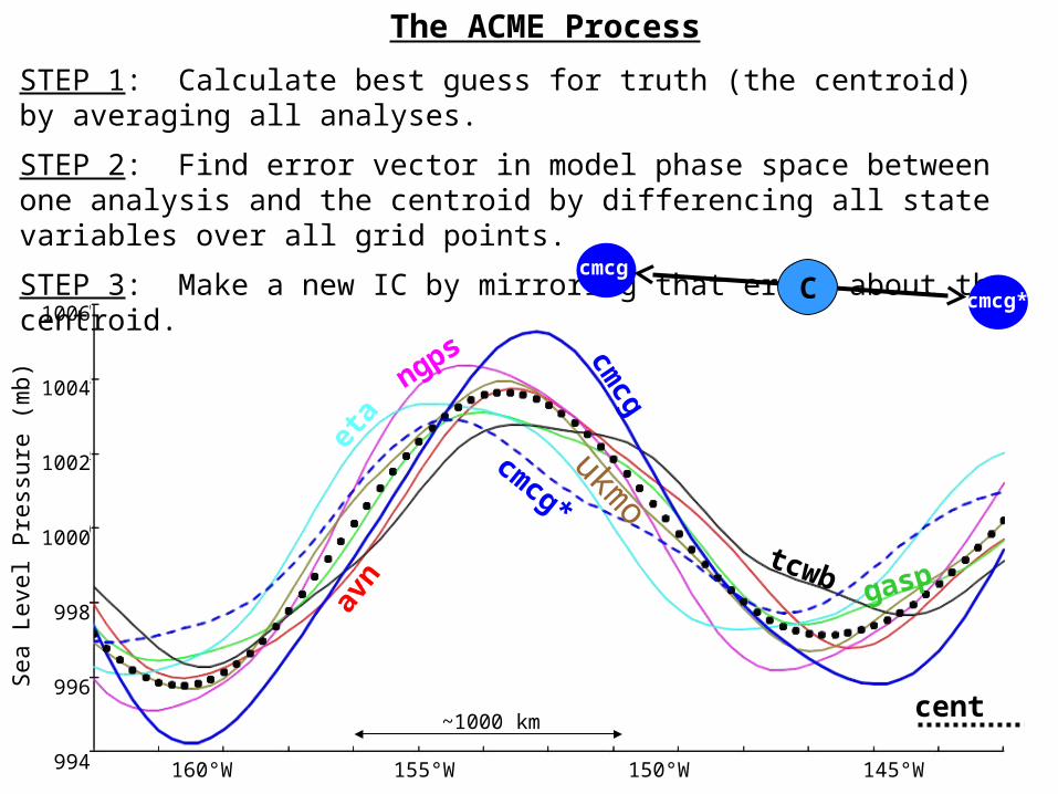
The ACME Process
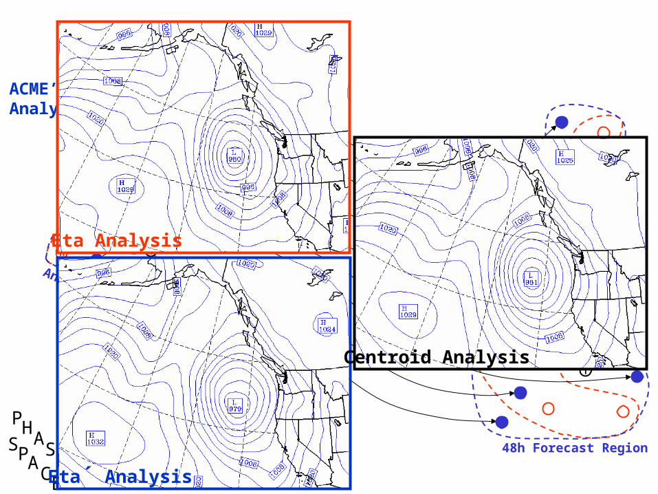
STEP 1: Calculate best guess for truth (the centroid) by averaging all analyses.
STEP 2: Find error vector in model phase space between one analysis and the centroid by differencing all state variables over all grid points.
STEP 3: Make a new IC by mirroring that error about the centroid.
cmcgC cmcg*
Sea
Lev
el P
ress
ure
(mb)
~1000 km
1006
1004
1002
1000
998
996
994
cent
170°W 165°W 160°W 155°W 150°W 145°W 140°W 135°W
eta
ngps
tcwbgasp
avn
ukmo
cmcg
e
a
uc
j
tg
n
c
2 1 0 1 2 34
2
0
2
4
6
7
-2.96564
Core ,i 2
Cent ,1 2
32.5 ,Core ,i 1 Cent ,1 1
T
M
T
Analysis Region
48h forecast Region
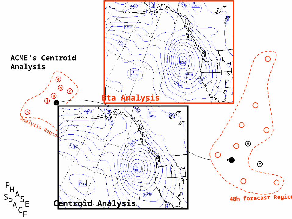
ACME’s Centroid Analysis
Eta Analysis
Centroid Analysis
PHA
SE
SPACE
PHA
SE
SPACE
e
n
ac
u
tg
T
j
T
Analysis RegionM
48h Forecast Region
e
a
uc
j
tg
n
c
2 1 0 1 2 34
2
0
2
4
6
7
-2.96564
Core ,i 2
Cent ,1 2
32.5 ,Core ,i 1 Cent ,1 1
ACME’s Mirrored Analyses
Eta Analysis
Eta´ Analysis
Centroid Analysis
1 2 3 4 5 6 7 8 9 10 11 12 13 14 15 16 17 1836h *ACMEcore0.0
0.1
0.2
0.3
0.4
1 2 3 4 5 6 7 8 9 10 11 12 13 14 15 16 17 1836h *ACMEcore0.0
0.1
0.2
0.3
0.4
0.4
0.3
0.2
0.1
0.01 2 3 4 5 6 7 8 9 10 11 12 13 14 15 16 17 18
36-h T2
36-h MSLP
*ACMEcore *ACME0.3
0.2
0.1
0.0
Comparison of Verification Rank Histograms
Verification Rank
Pro
bab
ilit
yP
rob
abil
ity
1 2 3 4 5 6 7 8 9 10 11 12 13 14 15 16 17 18
Verification Rank
1 2 3 4 5 6 7 8 9 10 11 12 13 14 15 16 17 18
36h *ACMEcore0.0
0.1
0.2
0.3
0.4
1 2 3 4 5 6 7 8 9 10 11 12 13 14 15 16 17 1836h *ACMEcore0.0
0.1
0.2
0.3
0.4
1 2 3 4 5 6 7 8 9 10 11 12 13 14 15 16 17 1836h *ACMEcore0.0
0.1
0.2
0.3
0.4
36-h WS10
MR = 52.5%MRE = 30.3%
VOP = 25.9%
MR = 44.0%MRE = 32.9%
VOP = 24.7%
*ACMEcore
*ACME
MR = 68.1%MRE = 45.9%
VOP = 44.4%
MR = 62.3%MRE = 51.2%
VOP = 44.2%
*ACMEcore*ACME
1 2 3 4 5 6 7 8 936h ACMEcore0.0
0.1
0.2
0.3
0.4
Pro
bab
ilit
y
0.4
0.3
0.2
0.1
0.01 2 3 4 5 6 7 8 9 10 11 12 13 14 15 16 17 18
Verification Rank
1 2 3 4 5 6 7 8 936h ACMEcore0.0
0.1
0.2
0.3
0.4
Pro
bab
ilit
y
0.3
0.2
0.1
0.01 2 3 4 5 6 7 8 9 10 11 12 13 14 15 16 17 18
36-h T2
MR = 36.5% MRE = 14.2%
VOP = 9.1%36-h MSLP
MR = 26.1%MRE = 15.0%
VOP = 8.7%
*ACMEcore
*ACME
1 2 3 4 5 6 7 8 936h ACMEcore0.0
0.1
0.2
0.3
0.4
Pro
bab
ilit
y
0.3
0.2
0.1
0.01 2 3 4 5 6 7 8 9 10 11 12 13 14 15 16 17 18
Verification Rank Histogramsfor…