Student thesis series INES nr 400

Sofia Sjögren

Effective Methods for Prediction and

Visualization of Contaminated Soil

Volumes in 3D with GIS

2016

Department of

Physical Geography and Ecosystem Science

Lund University

Sölvegatan 12

S-223 62 Lund

Sweden

ii

Sofia Sjögren (2016).

Effective Methods for Prediction and Visualization of Contaminated Soil Volumes in 3D with GIS

Effektiva metoder för att förutsäga och visualisera förorenade jordvolymer i 3D med hjälp av GIS

Master degree thesis, 30 credits in Geomatics

Department of Physical Geography and Ecosystem Science, Lund University

Level: Master of Science (MSc)

Course duration: January 2016 until June 2016

Disclaimer

This document describes work undertaken as part of a program of study at the University of Lund. All

views and opinions expressed herein remain the sole responsibility of the author, and do not

necessarily represent those of the institute.

iii

Effective Methods for Prediction and Visualization of

Contaminated Soil Volumes in 3D with GIS

Sofia Sjögren

Master thesis, 30 credits, in Geomatics

Supervisors:

Helena Eriksson,

Department of Physical Geography and Ecosystem Science, Lund University

Patrik Andersson,

Sweco Position

Exam committee:

Lars Eklundh, Department of Physical Geography and Ecosystem Science, Lund

University

Anton Lundkvist, Department of Physical Geography and Ecosystem Science,

Lund University

iv

Preface

This thesis has been written in cooperation with Sweco in Linköping. I would like to thank

my supervisor at Sweco, Patrik Andersson, for his time and valuable support. I would also

like to thank everyone else at the office for answering questions and their company. I would

like to thank my academic supervisor Helena Eriksson for her support throughout the project.

Finally, I want to say a big thank to my family for their great support. This project would not

have been possible to do without you.

2016-08-31

Sofia Sjögren

v

I. Abstract

Geographical Information Systems (GISs) have shown to be of great help in the work at

contaminated sites. Today there is an increase in the development of 3D modeling in many

fields. However, to combine the advantage working with spatial data in a GIS and 3D

modeling for subsurface soil data is limited. In this study, the possibilities of interpolating

volumes of soil contamination in 3D were investigated. The study is focused on the ability of

integrating 3D modeling with the GIS-environment in projects for contaminated land. Three

different interpolation techniques were evaluated; Kriging-, Inverse Distance Weighting

(IDW)-, and Nearest Neighbor interpolation. The data used in the study originates from a

contamination project at a former gasworks site in Norrköping, Sweden. The data was

sampled by the consultancy company Sweco. Three major contaminants of different

characteristics were evaluated for potential of volume interpolation in 3D (lead, benzene, and

polycyclic aromatic hydrocarbons (PAHs)). The study also aimed at determining if the

interpolation method with greatest potential differs in relation to contaminant type. Prior the

3D interpolation possible GIS software and other methods for 3D interpolation were

identified. Geostatistical analyses were performed where the optimized parameters for the

interpolations were determined. In the geostatistical analyses a spatial dependence at short

distances was found for all contaminants in the vertical direction (1-2 m) but not in the

horizontal plane. The lack of spatial dependence in the horizontal plane indicates an effect of

the coarse sampling density (about 10 m compared to 0.5 m for the vertical direction). The

distribution patterns of the three contaminants are expected. Lead and PAH are both

distributed differently depending on the soil material. Benzene seems to be distributed equally

in all material and was interpolated with the same parameters in all soil types. All

contaminants show greatest potential for volume interpolation with Kriging and secondly

IDW. The least accurate method was Nearest Neighbor. The optimized parameters for

interpolation are similar for lead and PAH but differed for benzene. That reflects their

difference in grade of mobility. Benzene shows the most accurate 3D volume interpolation

while PAH the least. It is suggested that an effective volume interpolation of pollutants in 3D

must combine regular GISs with software handling 3D volumes, or a development of the GIS-

software is necessary.

Keywords: 3D interpolation, 3D volumes, GIS, geostatistics, Kriging, remediation, soil

contamination

vi

II. Sammanfattning

Geografiska Informationssystem (GIS) har visat sig vara bra hjälpmedel i projekt för

förorenad mark. Idag utvecklas 3D-modellering inom många områden mer och mer. Att

kombinera 3D-modellering under markytan med fördelarna med att använda GIS för rumslig

data är däremot begränsad. I den här studien har möjligheterna till interpolering av förorenade

jordvolymer i 3D undersökts. Studien är fokuserad på integrering av 3D-modellering och GIS

i projekt för förorenad mark. De tre olika interpoleringsmetoderna Kriging, avståndsviktad

medelvärdesinterpolation (IDW) och närmaste-granne interpolering är undersökta. Det data

som används i studien kommer från ett markföroreningsprojekt vid ett gammalt gasverk i

Norrköping. Det är konsultbolaget Sweco som har tagit prover på jorden. Tre olika

markföroreningar med olika karaktär och som är viktiga i området undersöks för att utvärdera

möjligheterna till interpolering av volymer i 3D (bly, bensen och polycykliska aromatiska

kolväten (PAH)). I studien undersöks också om det är någon skillnad i bästa

interpoleringsmetoden beroende på typ av förorening. Innan 3D-interpoleringen utfördes

identifierades vilka möjliga metoder och GIS-program som är tillgängliga. Geostatistiska

analyser utfördes för att hitta de optimala parametrarna för interpoleringen. Ett kort rumsligt

samband (1-2 m) i vertikal riktning men inte i horisontell riktning hittades i de geostatistiska

analyserna för alla föroreningar. Avsaknaden av ett rumsligt samband indikerar en effekt av

den låga tätheten i provtagningen (10 m jämfört med 0,5 m i vertikal riktning).

Spridningsmönstret hos de tre föroreningarna är förväntat. Både bly och PAH har spridits på

olika sätt beroende på jordtypen. Bensen verkar ha samma spridningsmönster oavsett material

och interpolerades med samma parametrar i alla jordtyper. Resultatet från alla föroreningar visar på att Kriging ger den bästa volyminterpoleringen och IDW den näst bästa. Resultatet av

närmaste granne interpoleringen var minst korrekt. De optimala parametrarna för

interpolering är liknande för bly och PAH men annorlunda för bensen. Det reflekterar deras

olikheter i mobilitet. Bensen är den förorening med noggrannast resultat vid interpolering av

volymer medan PAH minst korrekt. Studien visar på att en effektiv 3D-interpolering av

föroreningar måste kombinera GIS med andra program som hanterar 3D-volymer, alternativt

krävs en utveckling av GIS-programvarorna.

Nyckelord: 3D-interpolering, 3D-volymer, geostatistik, GIS, Kriging, markföroreningar,

sanering

vii

Table of Contents

1. Introduction ................................................................................................... 1

2. Background .................................................................................................... 3

a) Contaminated Land ..................................................................................................................... 3

i) Soil Pollutants and their Characteristics .................................................................................. 3

ii) Environmental Pollutant Effects .............................................................................................. 5

iii) The Soil Remediation Process ................................................................................................. 6

b) Geostatistics ................................................................................................................................. 7

i) The Variogram ........................................................................................................................ 8

ii) Interpolation Techniques ....................................................................................................... 10

c) Geographical Information Systems (GISs) in Three Dimensions ............................................. 12

i) 3D Data Structures ................................................................................................................ 12

ii) 3D Software ........................................................................................................................... 13

3. Methods ........................................................................................................ 16

a) Site Description ......................................................................................................................... 16

b) Sampling Procedure .................................................................................................................. 17

c) Data ........................................................................................................................................... 18

d) Choice of Software .................................................................................................................... 18

e) Geostatistical Analysis .............................................................................................................. 19

f) 3D Interpolations ....................................................................................................................... 20

4. Results .......................................................................................................... 21

a) Geostatistical Analysis .............................................................................................................. 21

i) Statistical Analysis and Data Transformation ....................................................................... 21

ii) Trend Analysis ...................................................................................................................... 24

iii) Variogram Modeling ............................................................................................................. 26

iv) Soil Dependence .................................................................................................................... 30

v) Summary ............................................................................................................................... 32

b) 3D Interpolations ....................................................................................................................... 33

i) Validation .............................................................................................................................. 34

ii) Visualization and Implementation ......................................................................................... 36

5. Discussion ..................................................................................................... 42

a) Evaluation of 3D Interpolation Models ..................................................................................... 42

b) Evaluation on Contaminant Differences.................................................................................... 42

c) Evaluation on Methods for 3D Interpolation with GIS ............................................................. 43

d) Reliability of the Results and Future Research ......................................................................... 44

viii

6. Conclusion .................................................................................................... 45

7. References .................................................................................................... 47

1

1. Introduction

A major problem and important subject in the environmental protection field is the issue

concerning remediation of contaminated land. Today large areas around Europe are exposed

to contamination of soil and groundwater (Panagos et al., 2013). The contamination can be

harmful when spread to the ground, ecosystem or humans (Fent, 2004). The problem with

contaminated land is partly inherited from the past when the industrialization was intensive.

Industrial activities such as sawmills and gasworks utilized toxic substances. Contaminated

materials were used to level out or expand industry sites that today are abandoned. The

remnants from the industrial activities have led to contamination of the ground (Panagos et

al., 2013). Today urbanization and new developments demand for reusing the land for new

purposes. Prior to exploitation of a contaminated area the land must be remediated from

harmful levels of pollutants. Investigations and remediation of former industrialized sites are

expensive and time consuming projects (Brandon, 2013).

A core problem with remediation of contaminated land includes how to predict the

distribution of pollutants in the ground. How far and deep the pollutant is spread and to what

degree must be measured to decide on an appropriate remediation method. However, the

number of soil samples at a contaminated site is often limited. Moreover, every project

requires the commitment of financial and human capital. A highly prioritized goal in

remediation work is to find a method that is cost effective, and still accurate enough to

minimize the risk of spread to the humans and the environment.

Geographical Information Systems (GISs) and geostatistical methods are an aid in

determining pollution levels in soil volumes. Previous studies have shown that GIS-

technology and geostatistical methods are useful in the evaluation of contaminated sites for

characterizing contamination levels (Henshaw et al., 2004; Largueche, 2006; Henriksson et

al., 2013). Most geostatistical studies focus on the horizontal dimensions. However, soil

contamination is a three dimensional phenomenon. There is an advantage of working with

quantitative spatial data in GISs but it has been a slow development of integrating 3D

volumes (Abdul-Raman & Pilouk, 2008).

Another complicating factor for 3D evaluation at contaminated sites is the differences in

vertical and horizontal sampling densities. The soil is usually sampled in boreholes with a

high vertical sampling density and low horizontal sampling density. It is easy to take many

samples in each borehole but time consuming and expensive to drill many holes. GIS-based

systems for management of borehole data in 3D have been developed (Chen et al., 2002;

McCarthy & Granerio, 2006; Ranga Vital et al., 2015), although, these systems do not

visualize volumes of the data. The study of Delarue et al., (2009) applies a 3D approach for

soil horizons with a capability of 3D volume rendering. However, it is not built on

geostatistics and not applied on soil contaminants. Nevertheless, there are studies as Neteler

(2001), Piedade et al. (2014) and Wei et al. (2014) that show a great potential of predicting

soil contamination volumes in 3D.

The advances in computer technology allow for increasingly applied 3D models. There are

examples on various applications in studies of chemical dispersion in the atmosphere (Nichol

et al., 2010; Zahran et al., 2013). The advantages working with 3D models are that they

resemble the reality, and are more easily interpreted than 2D maps. The 3D evaluation are

historically and today common in mining geology and reservoir modeling (Mallet et al., 1989;

Cairns & Feldkamp, 1993; Chambers et al., 1999; Xikui et al., 2016) but rarer in soil science.

2

Hence, the application of subsurface volume models for contamination evaluation is still

scarce.

Sweco is a consultancy company that performs remediation and risk assessments of

contaminated sites. They are currently working with a project at the harbor in Norrköping,

Sweden (Sweco, 2015). The site has a complex contamination history due to industrial

activities and the utilization at former gasworks. Therefore, there is a need to increase the

information base at the contaminated site. Three contaminants have shown to be of

importance in the area; lead, benzene and polycyclic aromatic hydrocarbons (PAHs). These

are common soil pollutants expected to be found at former gasworks sites (Luthy et al., 1994).

Metals and PAHs are known as the most widespread contaminants around the world

(Swartjes, 2011). The three contaminants are also contaminants with different characteristics

regarding degradation and transportation in the ground.

A large amount of data is sampled and the use of GIS is well developed throughout the

remediation project at Sweco. The soil samples are collected as features with depth attributes

and other information of importance for each sample within a GIS. Today the contamination

levels are visualized as 2D maps or as 3D points. To get further information about the

contamination situation volume interpolation in 3D is requested. There is also a need for a

method for 3D interpolation to use in remediation projects. The method should preferably be

applicable within the work method with GIS in projects for contaminated sites.

Aim

The overall objective of this study is to investigate the possibilities to predict variations of soil

pollution levels from soil samples in 3D. Based on a preferable prediction model an aim is

also to investigate a work method for 3D interpolation and volume visualization in projects

for contaminated land. The study focuses on 3D interpolation from a GIS perspective.

The specific objectives of this study are:

Is it possible to predict 3D volumes of contaminated soil?

If so, which prediction model or interpolation method is preferable?

Does the preferred method depend on type of contaminant?

Propose a suitable methodology for performing analyses and visualizations of

contaminated soils in 3D.

To achieve the aim data sampled by Sweco at the contaminated area in Norrköping that will

undergo remediation is used as a case study. The three contaminants lead, benzene and PAH

are investigated. Geostatistical analyses of the contaminants are performed in order to find

suitable prediction parameters. Various interpolation methods in 3D are tested and evaluated,

both geostatistical and deterministic methods. The work method with projects for

contaminated sites and GIS at Sweco is studied, as well as suitable software and methods for

3D interpolation and visualization.

3

2. Background

a) Contaminated Land

The definition of contaminated land differs around the world. The European Environment

Agency define a contaminated site as “a potentially contaminated site in which the quantities

and/or concentrations of waste or harmful substances are such that – on the basis of the results

of risk assessment- they constitute danger to human health and/or the environment” (Prokop

et al., 2000). Soil contamination has mainly an anthropogenic source and is found in

proximity to cities (Swartjes, 2011). Local soil contamination is a result from intensive

industrial activities, insufficient waste disposal, mining, military activities or accidents that

have introduced excessive amounts of contaminants to the soil (Brandon, 2013).

Industrialization in more than 200 years in Europe has led to a widespread problem of soil

contamination. There are approximately 2.5 million sites in Europe where potential polluting

activities have occurred (Panagos et al., 2013). The Swedish Environmental Protection

Agency (Swedish EPA) estimates contaminated sites with high risk to about 8000 in Sweden.

Most are associated with past or present industrial activities (Naturvårdsverket, 2016).

Contamination from past industrial activities mainly originates from the time before 1970. At

that time there was not yet any environmental legislation or concern of contaminants

(Brandon, 2013).

i) Soil Pollutants and their Characteristics

Soil contamination can be constituted of inorganic and organic pollutants. The most common

pollutants in European soils and groundwater are heavy metals, mineral oils, chlorinated

hydrocarbons (CHC), PAHs, cyanides, phenols, and BTEX (benzene, toluene, ethylbenzene,

and xylenes) (Brandon, 2013).

Depending on contaminant it might end up in water by leaching through the soil to the

underlying groundwater, evaporate into the air or bind to the soil. The main processes

occurring when pollutants are introduced to the soil are:

Adsorption to soil particles; this is a process where the pollutant is bound to the

surface of a soil particle. The degree of adsorption is dependent on both the chemical

properties of the pollutant and the soil particle where pH is an important factor. Clay

minerals are for example in general adsorbing fewer amounts of heavy metals than

organic pollutants.

Evaporation to the atmosphere; the pollutant might volatilize into gaseous form and

evaporate into the atmosphere which most commonly occur with organic compounds.

Biological uptake or degradation; once the pollutants are in the ground they become

bioavailable to organisms in the soil that metabolizes the contaminant. The

contaminant might accumulate or degrade in the organism.

Abiotic degradation; the influences of light (photolysis) or water (hydrolysis) might

change the composition of the pollutant compound.

4

Transportation through the soil; the pollutants may diffuse down in the soil system

where main factors regulating the transportation are amount of infiltrating water, soil

pore space, and dimensions of the pollutant. At last the contaminant will end up in the

ground- or surface water.

The aggregative effect from these processes will decide the distribution in the ground system

and further transport to the hydrosphere, biosphere and atmosphere (Warfinge, 1997; Mirsal,

2008).

Lead

One of the most common heavy metals found at contaminated sites are lead (Pb) (Wuana &

Okieimen, 2011). Lead in surface soils origin from high-temperature processes such as lead

ore smelting, coal burning, and leaded petrol. In uncontaminated soils lead is present at

concentrations of < 20 mg/kg (Steinnes, 2013). Compared with many other pollutants lead has

a long residence time in the environment (Wuana & Okieimen, 2011). The tendency to

accumulate can be derived from the low solubility in water (Table 1) and that no microbial or

chemical degradation occurs (Steinnes, 2013).

The chemical behavior of lead has shown to be dependent on the content of organic matter. It

is strongly adsorbed to soil particles of humic matter, although that requires a pH in the soil

above 4. If organic material is absent, lead will bound to clay minerals. In mineral soils

adsorption occurs mainly on iron oxides. According to Steinnes (2013) lead is immobile in the

soil unless very high concentrations are present. The findings of Jensen (2005) show that the

first factor determining the bonding of lead in industrially contaminated soils are the

contamination levels.

Benzene

Benzene is an easily evaporated compound belonging to the group of volatile organic

compounds (VOCs). The main sources of benzene to the environment are petroleum and

chemical industries. The high volatility is the controlling physical property in the

environmental transportation of benzene. Benzene is highly mobile in the soil and easily

transported to the groundwater. This is due to its low adsorption capacity, although with a

higher organic content in the soil the adsorption of benzene to the soil tends to increase.

Other parameters that influence leaching potential include the soil type, amount of rainfall,

depth of the groundwater, and extent of degradation. Benzene is moderately soluble in water

and has a high vapor pressure (Table 1). In aerobic conditions benzene is biodegraded in the

soil (ATSDR, 2007a).

Polycyclic aromatic hydrocarbon (PAH)

PAHs are a group of organic compounds highly persistent and widespread in the environment.

The major source of PAHs is the incomplete combustion of organic material such as coal, oil

and wood and is commonly related to energy production. The PAHs consist of only carbon

and hydrogen compounds. They have two or more aromatic rings with a pair of carbon atoms

shared. PAHs that share up to six rings are called “small PAHs” and those with more than six

aromatic rings are called “large PAHs”. Polycyclic aromatic carbons are persistent in the

environment since they have high melting and boiling points, low vapor pressure, and have a

5

Table 1: Chemical properties of the studied contaminants lead, benzene and PAH

from ATSDR (1995, 2007a, 2007b) and general characteristics in the ground.

very low solubility in water (Table 1). The solubility and vapor pressure decreases with

heavier compounds and additional aromatic rings. In this investigation the group of large

PAHs is studied.

When the PAHs are introduced to the soil the major part will bound to soil particles and

become mobile. The factors that are influencing the grade of mobility is sorbent particle size

and pore size of the soil. If the PAHs are bound to particles that cannot move through the soil

then the mobility of PAHs are limited as well. The tendency to be adsorbed to soil particles

has been found to have the most significant correlation with organic carbon content (Abdel-

Shafy & Mansour, 2016).

ii) Environmental Pollutant Effects

Once contaminants are in the soil they can undergo chemical changes or degrade into toxic

products of different degrees (Fent, 2004). People can be exposed to soil contaminants

through ingestion (eating and drinking), skin contact or inhalation. The contaminant can

undergo bioaccumulation in the food chain; from a plant growing in the soil to an animal and

end up in humans (Wuana & Okieimen, 2011). Soil contaminants may be responsible for a

number of health effects from symptoms as skin eruption, to cancer and deaths. The

likelihood that health effects occur from exposure to soil contaminants depend on the toxicity,

how much of the contaminant is in contact with humans, how long and often the exposure

occurs (Swartjes, 2011).

In addition to possible health effects on humans, contamination of the ground can have

negative effect on the environment. Elevated levels of contaminants in the soil can harmfully

affect plant uptake, animal health, microbial processes and overall soil and groundwater

health. Contaminants may change plants metabolic processes and reduce yields or cause

visible damage to crops. Reduced plant uptake will decrease the food quality and the soils

usability for agricultural production. Contaminated groundwater that ends up in surface

waters will cause negative effects on aquatic organisms (Fent, 2004).

Lead Benzene PAHs

Chemical type Chemical formula

Heavy metal Pb

VOC C₆H₆

Organic compound C13-22H10-14

Molecular weight 207.2 78.11 152.2 - 276.3

Melting point 327.4 °C 5.5 °C 11 - 273 °C

Boiling point 1740 °C 80.1 °C 96.2 - 530 °C

Water solubility (at 25°C) Insoluble 1900 mg/L > 3.93 mg/L

Vapor pressure Soil adsorption Soil transportation Degradation in soil

2.77 mm Hg high (organic) immobile

low

75 mm Hg low

mobile moderate

> 0.00032 mm Hg moderate immobile

low

6

Table 2: The general steps performed in projects

for soil remediation (Mirsal, 2008).

iii) The Soil Remediation Process

The term ‘soil remediation’ refers to actions designed to eliminate or reduce the risk

associated with contaminated sites (Carlon et al., 2009). A soil remediation project is

performed if contamination of a site can be suspected due to the history and past activities.

The remediation processes differ depending on type of site and remediation aim. However,

there are a variety of general steps performed in all projects for cleaning up contaminated sites

(Table 2). These are performed at Sweco and also presented in Mirsal (2008).

General steps in soil remediation projects

1) Site information gathering

2) Creating sampling plan

3) Field sampling

4) Lab analysis 5) Risk assessment and description of

contamination situation

6) Remediation action

The preliminary preparation in a soil remediation project (step 1, Table 2) is to collect all

available information of a contaminated site in order to characterize it. The geographic and

geologic conditions are reviewed as well as photographs, maps, and data about previous land

use activities. A sampling plan is determined to form the framework of the data collection

(step 2, Table 2). The sampling design and sampling locations are dependent on the sampling

purpose, topography and geologic conditions of the area. A common design is to specify a

grid with equal space covering the investigation area. In each grid cell either a systematic or

random sampling pattern is applied.

The soil and groundwater in the contaminated area are sampled (step 3, Table 2). The samples

are then sent to a lab for analysis of their chemical concentrations (step 4, Table 2). These

results are the information basis to specify the spatial dimensions of the contamination (step 5,

Table 2). The analyses of the soil and ground water samples are the foundation for a risk

assessment. The general purpose of a risk assessment is to estimate the risks associated with a

contaminated site. It aims to evaluate to what degree the risks need to be minimized

(Naturvårdsverket, 2009a).

In Sweden, generic guideline values that should not be exceeded are defined by the Swedish

EPA (Naturvårdsverket, 2009b). Risk values for two types of land use are defined; ‘sensitive

land use’ and ‘less sensitive land use’. At sites with sensitive land use contamination levels

should not limit activities for residents, agriculture, and schools. Additionally, surface- and

ground water should be protected from contamination in areas classified as sensitive land use.

Areas defined as less sensitive land use should allow for activities like commerce, industry,

and transport facilities. The generic guideline values for the studied contaminants are shown

in Table 3. In the risk assessment the sampled contamination concentrations are compared to

the generic guideline values (Naturvårdsverket, 2009a).

7

Table 3: The generic guideline values for the studied contaminants

lead, benzene, and PAH (Naturvårdsverket, 2009b).

Sensitive land use (mg/Kg)

Less sensitive land use (mg/Kg)

Lead 50 400 Benzene 0.012 0.04 PAH 1 10

At last an action for reducing the risk or other necessary measures is designed (step 6, Table

2). There are a variety of available remediation methods; removal of the soil, in-situ- and ex-

situ methods. The action used is a trade-off between the degree of remediation desired to

lower the exposure for humans and the environment, what is technically possible to

accomplish and economically reasonable (Carlon et al., 2009).

b) Geostatistics

Geostatistics is a set of statistical techniques used in the analysis of georeferenced data that

can be applied to environmental contamination and remediation studies. The geostatistical

theory originates from the gold mining industry where it evolved from requirements for

improved prediction of gold grades in the 1960s. The application incorporates location, spatial

relationships and classical statistics into the estimation process (Goovaerts, 1997).

Matheron (1963) developed the geostatistical techniques and introduced the concept

regionalized variables. According to the theory regionalized variables exhibit a statistically

measurable degree of continuity within a limited region. Within that region a statistical

relationship between the value of a pair of regionalized variables and their distance apart can

be determined. At greater distances the difference should be statistically independent of each

other (Matheron, 1971). The theory of the regionalized variables was later stated in Tobler’s

first law of geography ‘Everything is related to everything else, but near things are more

related than distant things’ (Tobler, 1971).

If the spatial variation (or spatial autocorrelation) of a regionalized variable can be

determined, then that information can be used to predict the values at unknown locations. A

regionalized variable has a spatial variation that is unknown but its variability with respect to

distance is statistically measurable within a finite area. An underlying assumption in

geostatistics is that the regionalized variables have a statistical normal distribution (Houlding,

2000).

8

i) The Variogram

Variogram modeling is an analysis for establishing the variance of regionalized variables and

the distance between them (Houlding, 2000). Samples are divided into lags (distances

intervals) to compute the variogram and determine the variance. Sample pairs in each lag with

similar distances are compared. The variogram can be derived from the equation (1) of semi-

variance.

𝛾(ℎ) = 1

2𝑝∑ (𝑧𝑖

𝑝𝑖=1 − 𝑧𝑖+ℎ)2 (Equation 1)

where

𝛾(ℎ) is the semivariance in lag ℎ,

𝑝 is the number of sample pairs within the lag ℎ,

𝑧𝑖 is the measured value of sample 𝑖, and

𝑧𝑖+ℎ is the measured value for a sample within the lag distance ℎ from sample 𝑖 (Goovaerts,

1997).

Each lag distance in the variogram must be large enough to contain a sufficient number of

pairwise sample comparisons and small enough for detecting the spatial variability. Figure 1a

shows a typical appearance of a variogram with a determined spatial variability. Such

variogram has three properties; a sill, range and a nugget. The sill is the semi-variance value

where the spatial variance ends. The range is the lag distance at which the spatial variance

ends. The nugget is the noise in the data or variability in the data at distances smaller than the

sampling space. Figure 1b shows a variogram where the spatial variability is random and

independent from the distance (Isaaks & Srivastava, 1989).

Geostatistical interpolation methods need to replace the experimental variogram (points in

Figure 2) with a variogram model (lines in Figure 2). Variogram values for lag distances that

are not computed (between the points) need to be accessed. Spherical, experimental and

Gaussian models are the most frequent used. These are commonly fitted by an iterative least

squares estimation. As seen in Figure 2 the different models result in different properties for

the sill, range and nugget (Goovaerts, 1997).

Figure 1a: A characteristic appearance of a vario-gram with a detected spatial autocorrelation, and its properties; range, sill and nugget.

Figure 1b: A characteristic appearance of a variogram from a random process without detection of any spatial variability.

Figure 1a-b adopted and modified from Hengl (2007)).

9

Within a region the sampled values can have different spatial variance in different directions.

This is called anisotropy. To determine if anisotropy exists in a dataset the variogram must be

computed in different directions. If the spatial variability only depends on the lag distance the

variogram is isotropic (Figure 3a). If the variogram changes with respect to both lag distance

and direction (Figure 3b) the variogram is anisotropic (Manto, 2005).

There are two kinds of anisotropy; geometric and zonal anisotropy. Zonal anisotropy occurs

when the sill of a variogram changes in different directions. Geometric anisotropy is a more

common model for anisotropy. The geometric anisotropy variogram reaches the same sill in

all directions but at different ranges. That implies a stronger correlation in one direction than

in other directions (Goovaerts, 1997). Directions in both the plane and vertical direction must

be considered when working with subsurface data. Geometric anisotropy is commonly

occurring in geological settings due to stratification of different soil material. In such a setting

the vertical variogram reaches the sill at much shorter distances than the horizontal variogram

(Bohling, 2005).

Figure 3a: An example of an isotropic vario-gram that does not vary in different directions.

Figure 3b: An example of an aniso-tropic variogram that has different variogram properties in different directions.

Figure 2: An example of three different variogram models (Spherical, Exponential, and Gaussian) fitted to a variogram (Adopted and modified from Goovaerts (1997)).

Exponential

10

Plotting the directional ranges of a variogram with geometric anisotropy in 3D space they

would fall on the surface of an ellipsoid (Figure 4a). The major and minor axes of the

ellipsoid correspond to the largest and shortest ranges of the directional variogram. Six

parameters are needed to specify the ellipsoid: three ranges (ℎ𝑥, ℎ𝑦, ℎ𝑧) and three rotation

angles (𝑎𝑥, 𝑎𝑦, 𝑎𝑧) to quantify orientation in a coordinate system (Manto, 2005).

Geostatistical interpolation methods are based on isotropic variogram models. To implement

such interpolations correction for anisotropic structures are necessary. The six parameters

defining the ellipsoid of anisotropic variogram can be used to transform it to an isotropic one.

A three-dimensional lag vector can be transformed into an equivalent isotropic lag vector (ℎ)

(Equation 2). Plotting the ranges in 3D space after the transformation they would correspond

to a sphere (Figure 4b) (Bohling, 2005).

ℎ = √(ℎ𝑥

𝑎𝑥)

2

+ (ℎ𝑦

𝑎𝑦)

2

+ (ℎ𝑧

𝑎𝑧)

2

(Equation 2)

ii) Interpolation Techniques

There are various techniques available for predicting values between locations of existing

samples. Some of them are more sophisticated and based on statistical analysis and

geostatistics while others are deterministic and based on subjective parameters. The simplest

form of interpolation is the average value of all sampled points. The equation (3) for the

weighted average value is the foundation for the more sophisticated interpolations.

�̂�𝑝 = ∑ 𝜆𝑖×𝑧𝑖

𝑛𝑖=1

∑ 𝜆𝑖𝑛𝑖=1

(Equation 3)

where

�̂�𝑝 is the interpolated value in point p,

n is the number of observed samples,

𝑧𝑖 is the attribute value of sample i,

𝜆𝑖 is the weight of 𝑧𝑖

The mean value interpolation has a 𝜆𝑖 value of 1 for all sample observations.

Figure 4a: An ellipsoid corresponding to the ranges from an anisotropic variogram in 3D space.

Figure 4b: A sphere corresponding to the variogram ranges from an isotropic variogram in 3D space (adopted and modified from Manto (2005)).

11

Nearest Neighbor

The Nearest Neighbor interpolation assigns an interpolated value to an unknown point the

same value as the nearest sampled point. It is an area based method where Thiessen polygons

are created around the sampled value. The method aims to preserve the local differences. In a

three dimensional approach if the vertical sampling resolution is denser than the horizontal a

scale effect can be added to reduce the resolution differences. In this case all the weight (𝜆𝑖)

in Equation 3 are given to the Nearest Neighbor of a sampling point. It is a simple form of

interpolation where no further parameter needs to be assigned to the Nearest Neighbor.

Splines

Another deterministic group of interpolation techniques are based on splines. A spline is a

type of piecewise polynomial that generates smooth, curved lines that can be conformed to a

smooth surface. The interpolated values in spline interpolation are not adapted to the

measured values to avoid local maximum and minimum values. This method aims to keep the

global smoothness. There are many versions of spline interpolation where one of the most

widely used is regularized spline with tension and smoothing (RST) (Mitášová and Mitáš,

1993). The RST interpolation is deterministic in the way that both a smoothing and a tension

parameter need to be determined. The equation for RST can be obtained from Mitášová and

Mitáš (1993).

Inverse distance weighting (IDW)

IDW interpolation is another deterministic interpolation technique described by Shepard

(1968). IDW interpolation gives a weight for each measured sample inversely proportional to

its distance from the point being interpolated. The principle of using inverse distances are

based on Tobler’s first law of geography (Tobler, 1970), and emphasizes the spatial similarity

of near points.

The equation for IDW interpolation is similar to the mean value (Equation 3). However, the

weight (𝜆𝑖) in Equation 3 is equal to the inverse of the distance from sample i to point p (1

𝑑𝑖𝑘).

k is an estimated weight exponent for the spatial dependence. The exponent k decides how

strong the influence of near points should be. A high value of k corresponds to a strong spatial

influence. Another factor influencing the values of the interpolated points is the search radius

and how many points that should be included in the interpolation. The search radius in both

horizontal and vertical directions must be considered when interpolating subsurface data at

different depths (Isaaks & Srivastava, 1989).

Kriging

Kriging is a geostatistical interpolation method for optimal spatial estimation. It was first

published by Krige (1951). The Kriging interpolation is more advanced than previous

mentioned interpolation methods and requires a geostatistical analysis and variogram

modeling before it can be applied. Kriging interpolation produces more objective maps, and

apart from interpolating based on the spatial autocorrelation it can produce an error estimation

of the prediction.

The simplest form of Kriging and most commonly applied is called ‘Ordinary Kriging’. In

Kriging interpolation the weights (𝜆𝑖) in Equation 3 is based on the variogram properties. The

12

kriging algorithm will give more importance to semi-variance values with a large number of

sample pairs and at short distances (Oliver, 2009). Important requirements for Ordinary

Kriging interpolation are that no trend exists in the data, the variogram is constant in the

studied area, and that the interpolated value follows a normal distribution (Hengl, 2007).

c) Geographical Information Systems (GISs) in Three Dimensions

GISs are tools for capturing, storing, manipulating, and analyzing data with a spatial

dimension. Many GISs used within geoscience are based on two-dimensional (2D) or two-and

a half-dimensional (2.5D) spatial data. Spatial objects are represented in the form of vector

points, lines, polygons and raster surfaces. A general GIS has difficulties managing and

visualizing geographical data with a greater dimension. There are limits in 3D representation

of such data since multiple z-values cannot be displayed within the same surface (Figure 5).

Samples from the subsurface and borehole data have in most cases multiple z-values at the

same location. Therefore, for a general GIS there are limitations in subsurface geologic

modeling (Abdul-Rahman & Pilouk, 2008). To find boundary and limits of soil contamination

there is a need of representing the samples as volumes rather than surfaces. Subsurface data

requires exploratory interpolation tools that traditionally are not part of a GIS (Setijadji,

2003). GIS software that handles 3D representations is rarer due to the complexity of the 3D

data structure (Abdul-Rahman & Pilouk, 2008).

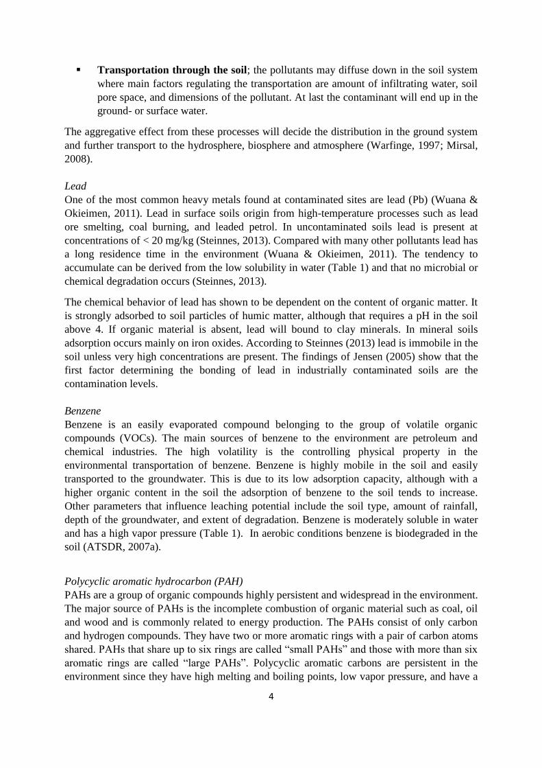
i) 3D Data Structures

In a GIS the most common and simple data structure representing a volume or a body is the

“voxel”. The term voxel represents “volume”, “pixel” and “element”. That is a regular 3D

grid of cells, each with its unique attributes and coordinates (Figure 6a). Typically these data

structures are stored as a one-dimensional array of element (Abdul-Rahman & Pilouk, 2008).

Each element is defined by the x, y, and z coordinates of the voxel centroid. Each voxel

centroid in the data structure represents a finite equal volume. In that way the 3D grid

simulates a spatially continuous measure of a variable. That by assigning values which are

representative of a determined, small volume to points at regular intervals. One disadvantage

of this data structure is that it requires large computer space for a high resolution grid

(Houlding, 2012).

Figure 5: A 3D surface and samples with multiple z-values that are not represented in the surface.

13

A more sophisticated form of the 3D grid structure is the Octree (Figure 6b). The Octree

structure allows for irregular voxels with different sizes. The Octree voxels are stored in a tree

data structure. The root in the tree structure is conceptually a “universe cube” containing all

voxels in the object. The cube has eight nodes representing eight identical cubes inside the

root cube called octants. These cubes can either be inside or outside the object. Each octant is

subdivided into eight octants repetitively until the smallest size of the object is represented

(Abdul-Rahman & Pilouk, 2008).

Constructive solid geometry (CSG) is a way of representing objects as predefined geometric

solids (Figure 6c). These could be spheres, cubes, cylinders etc. and are more commonly used

in solid 3D modelling such as CAD (Mallet, 1992), and will not be presented further in this

study.

Another way of representing 3D volumes in GIS is a 3D tetrahedral network (TEN) (Figure

6d). That is an extension of the 2D triangular network (TIN). An object is described by

connected tetrahedral with four vertices, six edges, and four faces. The TEN structure has the

advantage of having a simple data structure and fast topological structure. However, the

representations of TENs in many GIS are limited (Abdul-Rahman & Pilouk, 2008).

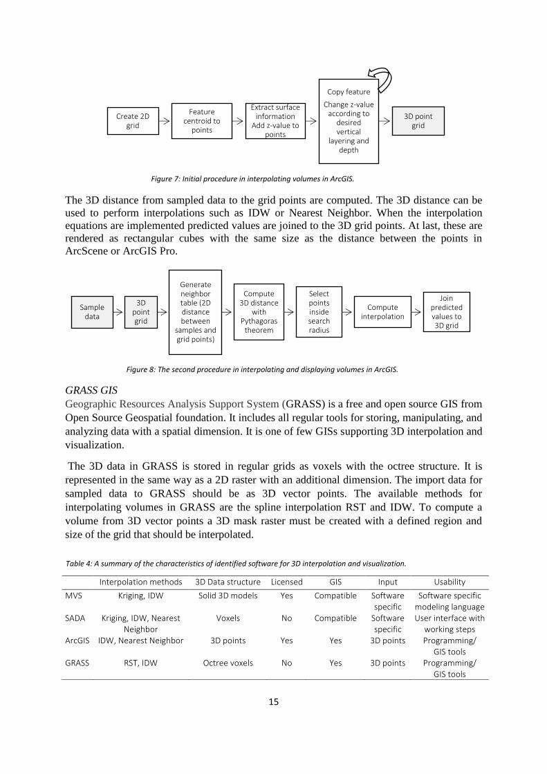
ii) 3D Software

In the following section examples of identified software for interpolation and visualization of

3D soil contamination volumes are presented. A further overview of geostatistical 3D

software is found in Goovaerts (2009). Table 4 summarizes the general characteristics of the

identified software.

Mining Visualization System (MVS)

C´Techs Mining Visualization System (MVS) is a solid 3D modeling software for

visualization of subsurface data. It is used as extension to a GIS for computing and visualizing

3D models. MVS is just one of many solid 3D modeling software and it is not the only one

concentrated on subsurface data. This kind of software is in general licensed and expensive.

Figure 6a: The voxel data structure of with cells in a regular 3D grid.

Figure 6b: The Octree data structure allowing for varying sizes of the 3D cells.

Figure 6c: The constructive solid geometry (CSG) data structure used in 3D modeling.

Figure 6d: The tetrahedral network (TEN) data structure for trianulated representations of 3D data.

Figures 6a – 6d adopted and modified from Xikui et al. 2016.

14

MVS uses its own type of modeling language to perform operations. It is a visual

programming environment where modules are connected in a flow chart of input and output

ports. Necessary inputs are coordinates, elevation, surface elevation, and contaminant

concentrations for a chosen number of contaminants. To compute volumes MVS perform

Kriging interpolation. The computation is completely automated where no previous

knowledge from the user is needed. That is, without specifying any parameters the optimal

variogram and Kriging interpolation is performed according to the system. However, there are

options for specialists with knowledge of the data to manipulate the variogram variables.

MVS displays the data in a format of a regular grid. For example, there are options for

visualizing soil pollution concentrations in different geological layers and as volumetric

plumes of certain soil pollution concentrations (C’Tech, 2015).

SADA

Spatial Analysis and Decision Assistance (SADA) is a freeware program developed at the

University of Tennessee. It is designed for environmental characterization and remediation.

The functionalities of SADA are multidisciplinary and provide tools recognized from a GIS

but include also sampling design, risk assessment, remedial design, and cost/benefit analysis.

SADA comes with the possibilities of 2- and 3D interpolation and visualization (Purucker et

al., 2009).

The available 3D interpolation methods in SADA are: Nearest Neighbor, IDW, Ordinary

Kriging, Ordinary Cokriging, and Indicator Kriging. The input to SADA requires a strict

format where only one contaminant can be imported at the time. No elevation surface is used,

the samples are computed as depth below the surface. The workflow for computing volumes

and visualize the data in SADA is an approach where the user is lead through a number of

steps. At first the site is set up, and grid spacing and vertical layers are defined. The grid and

vertical layers defines the voxels used to visualize the data. An interpolation method is chosen

and parameters are specified. In Kriging interpolation the variogram must be computed and

the optimal parameters defined. SADA suggest default values for the variogram but these are

not intended to be the optimal ones (SADA, 2005).

ArcGIS

ArcGIS is one of the most developed and widespread GISs in various fields. It is a group of

software routines developed by Environmental Sciences Research Institute (ESRI). ArcGIS

requires a license but in Sweden many municipalities and consultancy companies have access

to the software. The most common ArcGIS software is ArcMap that handles and visualizes

geospatial information in 2D. In the software ArcScene and ArcGIS Pro the data can be

visualized in 3D as well. ArcGIS does not have a data type for volumes but can still render

data in 3D. The outputs of the 3D analysist tools found in the software are 2.5D surfaces and

not volumes.

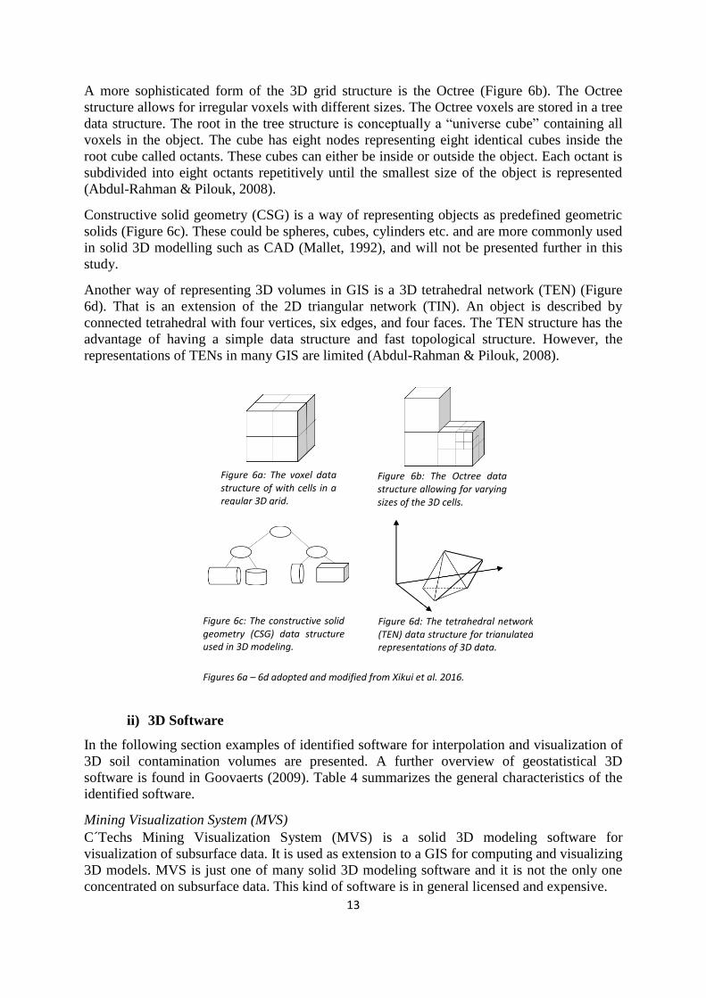
The software can be manipulated to perform 3D interpolation and then render points as 3D

cubes. A proposed method for volume interpolation and visualization is presented in figures 7

and 8. At first a 3D point grid is created at the site to be interpolated. It is created from a 2D

grid that is copied with changing z-values for the desired depth.

15

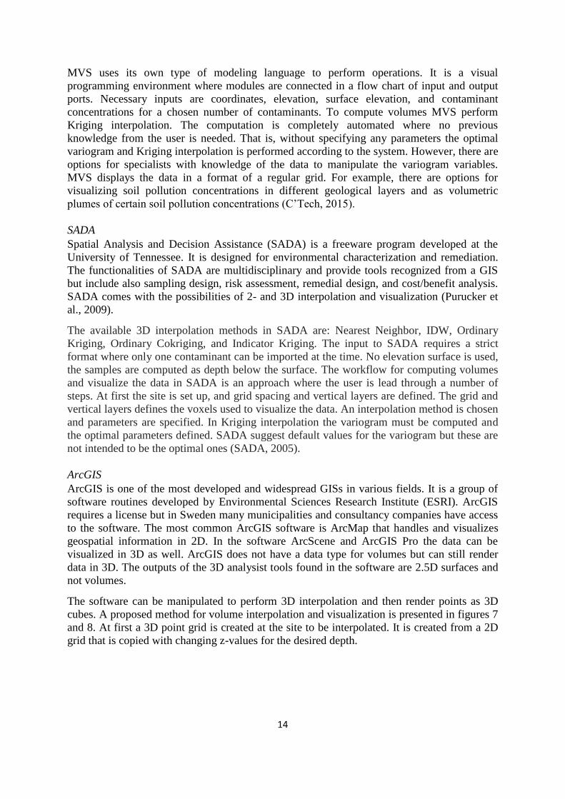
The 3D distance from sampled data to the grid points are computed. The 3D distance can be

used to perform interpolations such as IDW or Nearest Neighbor. When the interpolation

equations are implemented predicted values are joined to the 3D grid points. At last, these are

rendered as rectangular cubes with the same size as the distance between the points in

ArcScene or ArcGIS Pro.

GRASS GIS

Geographic Resources Analysis Support System (GRASS) is a free and open source GIS from

Open Source Geospatial foundation. It includes all regular tools for storing, manipulating, and

analyzing data with a spatial dimension. It is one of few GISs supporting 3D interpolation and

visualization.

The 3D data in GRASS is stored in regular grids as voxels with the octree structure. It is

represented in the same way as a 2D raster with an additional dimension. The import data for

sampled data to GRASS should be as 3D vector points. The available methods for

interpolating volumes in GRASS are the spline interpolation RST and IDW. To compute a

volume from 3D vector points a 3D mask raster must be created with a defined region and

size of the grid that should be interpolated.

Interpolation methods 3D Data structure Licensed GIS Input Usability

MVS Kriging, IDW Solid 3D models Yes Compatible Software specific

Software specific modeling language

SADA Kriging, IDW, Nearest Neighbor

Voxels No Compatible Software specific

User interface with working steps

ArcGIS IDW, Nearest Neighbor 3D points Yes Yes 3D points Programming/ GIS tools

GRASS RST, IDW Octree voxels No Yes 3D points Programming/ GIS tools

Sample data

3D point grid

Generate neighbor table (2D distance between

samples and grid points)

Compute 3D distance

with Pythagoras

theorem

Select points inside search radius

Compute interpolation

Join predicted values to 3D grid

Figure 8: The second procedure in interpolating and displaying volumes in ArcGIS.

Create 2D grid

Feature centroid to

points

Extract surface information

Add z-value to points

Copy feature

Change z-value according to

desired vertical

layering and depth

3D point grid

Figure 7: Initial procedure in interpolating volumes in ArcGIS.

Table 4: A summary of the characteristics of identified software for 3D interpolation and visualization.

16

3. Methods

a) Site Description

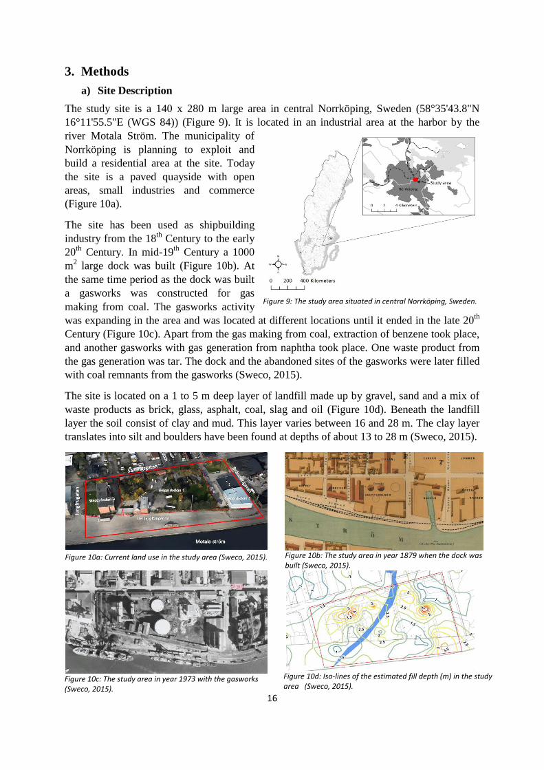
The study site is a 140 x 280 m large area in central Norrköping, Sweden (58°35'43.8"N

16°11'55.5"E (WGS 84)) (Figure 9). It is located in an industrial area at the harbor by the

river Motala Ström. The municipality of

Norrköping is planning to exploit and

build a residential area at the site. Today

the site is a paved quayside with open

areas, small industries and commerce

(Figure 10a).

The site has been used as shipbuilding

industry from the 18th

Century to the early

20th

Century. In mid-19th

Century a 1000

m2 large dock was built (Figure 10b). At

the same time period as the dock was built

a gasworks was constructed for gas

making from coal. The gasworks activity

was expanding in the area and was located at different locations until it ended in the late 20th

Century (Figure 10c). Apart from the gas making from coal, extraction of benzene took place,

and another gasworks with gas generation from naphtha took place. One waste product from

the gas generation was tar. The dock and the abandoned sites of the gasworks were later filled

with coal remnants from the gasworks (Sweco, 2015).

The site is located on a 1 to 5 m deep layer of landfill made up by gravel, sand and a mix of

waste products as brick, glass, asphalt, coal, slag and oil (Figure 10d). Beneath the landfill

layer the soil consist of clay and mud. This layer varies between 16 and 28 m. The clay layer

translates into silt and boulders have been found at depths of about 13 to 28 m (Sweco, 2015).

Figure 9: The study area situated in central Norrköping, Sweden.

Figure 10b: The study area in year 1879 when the dock was built (Sweco, 2015).

Figure 10a: Current land use in the study area (Sweco, 2015).

Figure 10c: The study area in year 1973 with the gasworks (Sweco, 2015).

Figure 10d: Iso-lines of the estimated fill depth (m) in the study area (Sweco, 2015).

17

b) Sampling Procedure

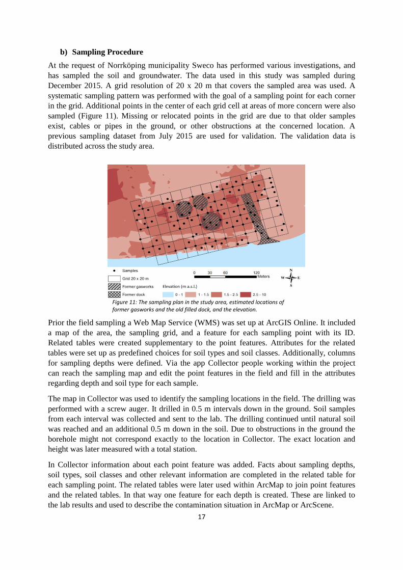
At the request of Norrköping municipality Sweco has performed various investigations, and

has sampled the soil and groundwater. The data used in this study was sampled during

December 2015. A grid resolution of 20 x 20 m that covers the sampled area was used. A

systematic sampling pattern was performed with the goal of a sampling point for each corner

in the grid. Additional points in the center of each grid cell at areas of more concern were also

sampled (Figure 11). Missing or relocated points in the grid are due to that older samples

exist, cables or pipes in the ground, or other obstructions at the concerned location. A

previous sampling dataset from July 2015 are used for validation. The validation data is

distributed across the study area.

Prior the field sampling a Web Map Service (WMS) was set up at ArcGIS Online. It included

a map of the area, the sampling grid, and a feature for each sampling point with its ID.

Related tables were created supplementary to the point features. Attributes for the related

tables were set up as predefined choices for soil types and soil classes. Additionally, columns

for sampling depths were defined. Via the app Collector people working within the project

can reach the sampling map and edit the point features in the field and fill in the attributes

regarding depth and soil type for each sample.

The map in Collector was used to identify the sampling locations in the field. The drilling was

performed with a screw auger. It drilled in 0.5 m intervals down in the ground. Soil samples

from each interval was collected and sent to the lab. The drilling continued until natural soil

was reached and an additional 0.5 m down in the soil. Due to obstructions in the ground the

borehole might not correspond exactly to the location in Collector. The exact location and

height was later measured with a total station.

In Collector information about each point feature was added. Facts about sampling depths,

soil types, soil classes and other relevant information are completed in the related table for

each sampling point. The related tables were later used within ArcMap to join point features

and the related tables. In that way one feature for each depth is created. These are linked to

the lab results and used to describe the contamination situation in ArcMap or ArcScene.

Figure 11: The sampling plan in the study area, estimated locations of former gasworks and the old filled dock, and the elevation.

18

Table 6: A summary of the software used in the study.

Table 5: A summary of the data used in the study.

c) Data

The data used in the study is summarized in Table 5. In total 763 samples from 126 boreholes

were used. The validation dataset consist of 188 samples. The validation data has a mean

depth of 1.9 m and maximum depth of 2.9 m. An elevation model was used for surface height

information.

Data Type Coordinate System Projection Origin

763 samples Feature class

SWEREF 99 TM SWEREF 99 1630 Field sampling, 12-2015 (Sweco)

188 validation samples Feature class

SWEREF 99 TM SWEREF 99 1630 Field sampling, 07-2015 (Sweco)

Elevation model TIN SWEREF 99 TM SWEREF 99 1630 Laser scanning (Sweco)

d) Choice of Software

SADA was chosen for the computation of 3D interpolations (Table 6). In SADA it is possible

to define the parameters that should be used in the computation. Moreover, SADA allows for

evaluation of many different interpolation methods, both geostatistical and deterministic

methods which was not possible in the other software (Table 4). It was also the only

comprehensive software available where no programming or license is necessary.

Prior the interpolations, the statistical and geostatistical analyses were performed in R and the

subprogram Rstudio (Table 6). R allows for handling data in three dimensions. With the

GSTAT package it is also possible to compute variogram models in three dimensions

(Pebesma, 2004). Beyond that, R is used due to the large freedom and control of the analyzed

data. Variogram computation is also available in SADA but R allows for more detailed and

controlled analyses necessary for some of the aims of the study.

The interpolated outcomes were later transferred back into ArcGIS (Table 6) for validation

and the subsequent visualization since the possibilities to control the data are limited in

SADA. The reason for that is to be able to use the validation dataset, combine the interpolated

outcome, and easily work with the data. ArcGIS was used for visualization to avoid more data

processing than necessary. To keep the data in ArcGIS allows for continuous data processing

at Sweco and further risk assessments.

Software Application Origin

Rstudio Statistical and geostatistical analysis Rstudio Team (2015)

R 3.2.4 Statistical and geostatistical analysis R Core Team (2016)

SADA 5.0 3D interpolation, validation http://www.sadaproject.net/

ArcMap 10.3.1 Validation, 2D visualization http://www.arcgis.com/

ArcScene 10.3.1 3D visualization http://www.arcgis.com/

19

e) Geostatistical Analysis

The procedure to investigate the spatial dependence in the data is described in Figure 12 (step

a-e). At first, a statistical analysis is performed in R to get an idea of the distribution of the

data (a). Since the normal distribution is an underlying assumption in geostatistics the data

must be transformed if the data is skewed (b). Another underlying assumption is that there

should not be any trend in the data. The data is investigated to find any existing trend (c).

At last, variogram can be computed to look for any spatial dependence in the data, and if that

dependence is correlated (e-f). The variogram parameters that are determined in R are

described in Figure 13.

The covariance of the regionalized variable and the lagged regionalized variable is computed.

It is used to confirm the correlation and is computed with Equation 4.

𝐶(ℎ) =1

𝑛−1∑ (𝑧(𝑥𝑖) − 𝜇𝑛

𝑖=1 ) × (𝑧(𝑥𝑖 + ℎ) − 𝜇ℎ (Equation 4)

where

𝐶(ℎ) is the covariance in lag h

n is the number of samples in lag h

Figure 13: The parameters that should be determined in R for variogram computation are dip direction, plane direction, lag width, horizontal- and vertical tolerance.

Statistical Analysis (a)

Normal distribution? (b)

If yes; use the data

If no; transform the

data

Global trend? (c)

If yes; detrend and use residuals

If no; use mean

Geostatistical Analysis (d)

Compute Variogram (e)

Is the spatial dependence

correlated? (f)

If yes; fit variogrom

model

If no; no spatial

dependence

Figure 12: The method performed in steps from a to f in the geostatistical analysis and determine the spatial dependence of the data.

20

𝑧(𝑥𝑖) is the attribute value at location x of pair i

𝑧(𝑥𝑖 + ℎ) is the attribute value at location x + h of pair i

𝜇 is the mean value in the corresponding lag (Goovaerts, 1997).

Additionally, correlation with soil types and soil classes were investigated. If a significant

correlation was found it was investigated if the spatial dependence varied in different soils.

f) 3D Interpolations

The method from interpolation to implementation is described in Figure 14. 3D interpolations

are performed in SADA with parameters based on the geostatistical analysis. Three different

interpolation methods available in SADA were tested; Ordinary Kriging, IDW and Nearest

Neighbor. All parameters in the interpolations cannot be determined from the geostatistical

analyses. One of these was the length of the search radius which was tested for in the Kriging

and IDW interpolations. The IDW interpolation was also tested for different exponents,

whereas the Nearest Neighbor interpolation was tested for different vertical exaggerations.

The 3D distances between points that will be interpolated with new values must be

predefined. That is the thickness of the vertical layering and the horizontal grid spacing. The

grid spacing and layering should be set to 5-10 times smaller than the range, or in general one

fifth of the sampling density (Houlding, 2000). This was considered when deciding on the

resolution of the interpolations.

In SADA, the outcomes of the interpolations with different parameters were evaluated with

cross validation. In cross validation the interpolations are computed where one sample at the

time is excluded and then used for validation with the predicted value. From cross validation

an RMSE value can be obtained. The RMSE is a measure of the difference between sampled

data and predicted data. It is a common measure for validity prediction. The RMSE value was

computed using Equation 5 (Isaaks & Srivastava, 1989).

𝑅𝑀𝑆𝐸 = √1

𝑁∑ {𝑧(𝑥𝑖) − �̂�(𝑥𝑖)}2𝑁

𝑖=1 (Equation 5)

where

N, is the number of samples

z is the sampled value at location 𝑥𝑖

�̂� is the predicted value at location 𝑥𝑖

The predictions with parameters resulting in lowest RMSE from cross validation were chosen.

These were imported into ArcGIS for back transformation and adding the trend back for the

Kriging interpolations. The validation dataset was used to find the nearest interpolated values

in 3D distance from a validation sample. The value of the validation sample and the predicted

value were compared. The validity of the final predictions was obtained from the RMSE

value.

21

To see how the predicted contamination levels change with depth, the mean concentration of

each contaminant at different depths are computed. Lastly the predicted models for each

interpolation method and contaminant are visualized based on their risk levels. The

contaminated volumes are computed from the number of samples and their grid size.

4. Results

a) Geostatistical Analysis

In the following sections the outcomes of the statistical and geostatistical analyses are

presented.

i) Statistical Analysis and Data Transformation

The results from the lab analysis are shown in figure 16a-c and are based on the risk levels in

Table 3. The results are the foundation for the continued statistical analyses. There is a high

frequency of samples close to the surface and down to about 2.5 m (Figure 17). The sampling

frequency deeper than 4 m is less than 20 in each 0.5 m interval.

Figure 14: The procedure performed to interpolate the soil samples, optimize the parameters, and validate and visualize the results.

22

Figure 16a: The sampling and concentration distributions of lead.

Figure 16b: The sampling and concentration distributions of benzene.

Figure 16c: The sampling and concentration distributions of PAH.

Figures 16a-c: The classifications originate from Table 3. Less sensitive land and sensitive land are divided into two classes for each contaminant.

23

Table 7: Statistical summary of the sampled contaminants.

In Table 7 the descriptive statistics of the contaminant levels are presented. All three

contaminants have lower medians than mean values. That indicates positively skewed data.

That is a result of a high frequency of low concentrations and some exceptional high

concentrations in the datasets. This is a common distribution of soil contaminants (Juang et

al., 2001).

Lead

(mg/Kg) Benzene (mg/Kg)

PAH (mg/Kg)

Min. 0.55 0.00175 0.15 1st Quartile 9.2 0.00175 0.15 Median 18 0.00175 1.1 Mean 106.5 13.11 37.81 3rd Quartile 58.5 14 13 Max. 8300 130 1700 NA 8 0 8 Std 464.14 25.05 152.12 Variance 215426.2 627.26 23139.71

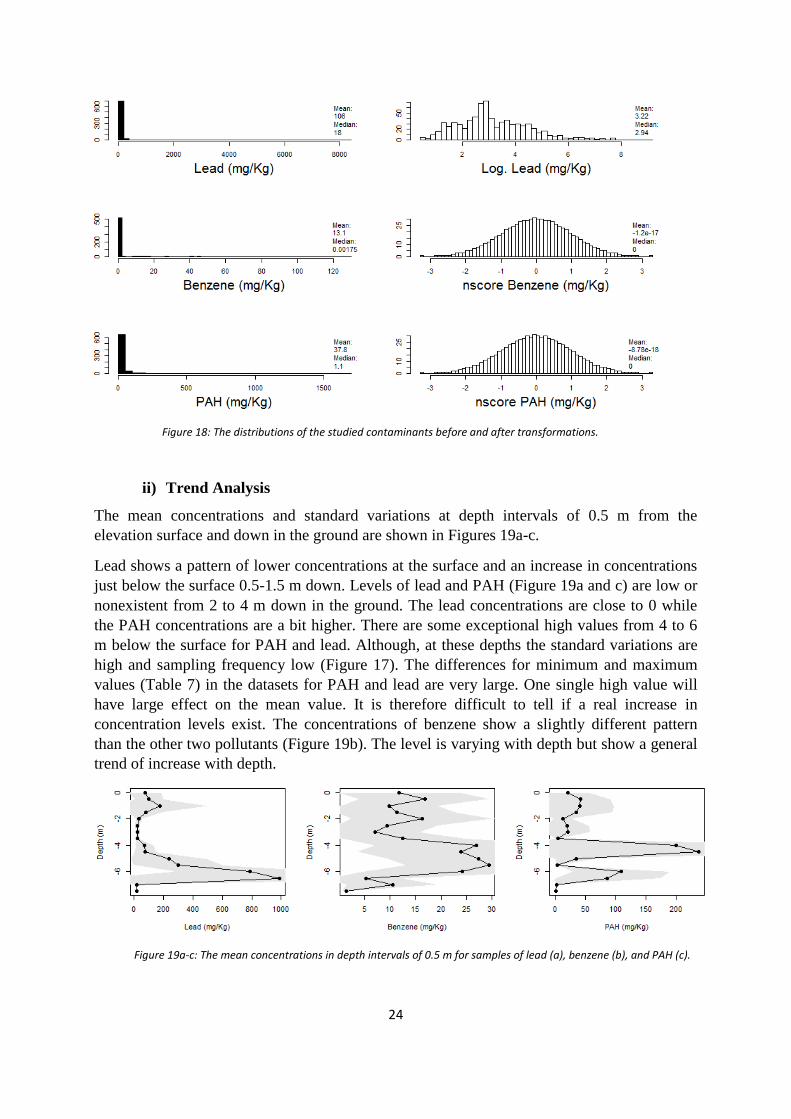
The skewed distributions of the data required a transformation (Figure 18). The most

commonly used transformation is the logarithmic transformation (Houlding, 2000).

Logarithmic transformations of the data result in a normal distribution for lead. The other two

contaminants were transformed with a normal score transformation. A normal score

transformation ranks the data from highest to lowest. The ranks are matched to equivalent

ranks generated from a normal distribution. The mean and median in a distribution of normal

scores are 0.

Figure 17: The sampling frequency in depth intervals of 0.5 m from the surface and down to a depth of 7.5 m.

24

ii) Trend Analysis

The mean concentrations and standard variations at depth intervals of 0.5 m from the

elevation surface and down in the ground are shown in Figures 19a-c.

Lead shows a pattern of lower concentrations at the surface and an increase in concentrations

just below the surface 0.5-1.5 m down. Levels of lead and PAH (Figure 19a and c) are low or

nonexistent from 2 to 4 m down in the ground. The lead concentrations are close to 0 while

the PAH concentrations are a bit higher. There are some exceptional high values from 4 to 6

m below the surface for PAH and lead. Although, at these depths the standard variations are

high and sampling frequency low (Figure 17). The differences for minimum and maximum

values (Table 7) in the datasets for PAH and lead are very large. One single high value will

have large effect on the mean value. It is therefore difficult to tell if a real increase in

concentration levels exist. The concentrations of benzene show a slightly different pattern

than the other two pollutants (Figure 19b). The level is varying with depth but show a general

trend of increase with depth.

Figure 19a-c: The mean concentrations in depth intervals of 0.5 m for samples of lead (a), benzene (b), and PAH (c).

Figure 18: The distributions of the studied contaminants before and after transformations.

25

A regression line is fitted to see if there is a trend in depth. As seen in figure 20a-c, visually

looking at the trend lines and the R2–values, there are no strong correlation with

concentrations and depths. The PAH concentrations are decreasing with depth as well as the

lead concentrations, although not that strong. Benzene behaves differently and indicates an

opposite trend or no trend at all in concentration level and depth. It needs to be considered

that the samples are clustered closer to the surface and less frequently sampled at deeper

levels (Figure 17).

Another analysis was performed to search for significant global trend surfaces in the area.

Linear trend surfaces and polynomial trend surfaces (degree 2) were fitted to the data in 3D.

As seen in Figure 21, all three contaminants have significant (*) trend surfaces at a 0.001

significance level. Benzene and PAH have significant trend surfaces for both linear and

polynomial trends. The residuals of the linear trend surfaces for benzene and PAH were used

in the continued analyses since the simplest trend is preferred. The residuals of the polynomial

trend surface for lead were used in the continued analyses.

Figure 20a-c: The concentrations variation with depth for samples of lead (a), benzene (b), and PAH (c), and their trend lines.

Linear, P-value: 1.1102e-15* Polynomial, P-value: < 2.22e-16*

Linear, P-value: 0.00047968* Polynomial, P-value: 1.6786e-10*

Linear, P-value: 0.57076 Polynomial, P-value: 0.0065445*

Figure 21: Linear and polynomial trend surfaces fitted to the three contaminants. The trend surfaces used in continued analysis are marked with dashed lines.

26

Table 9: The number of pairwise comparisons in each lag with the final variogram parameters.

Table 8: The parameters used in the variogram computation.

iii) Variogram Modeling

The parameters of the variogram are specified in Table 8, and were set to suit the sample

spacing in the studied area. The lag width for the variogram analyses in the vertical and

horizontal directions was set equal to the sampling spacing. The maximum distance to

compute semi-variance in was set to the maximum width and depth of the sampling area.

Various horizontal- and vertical tolerances (Figure 14) were tested to include a sufficient

amount of samples. Different dip- and plane directions were tested to detect any spatial

dependence in the area. The main directions are presented in Figures 22 and 23.

Horizontal Parameter

Vertical Parameters

Lag width 10 (m) 0.5 (m) Max. distance 250 (m) 9 (m) Direction in plane (x,y) 0° 0° Horizontal tolerance 30° 30° Dip direction (z) 0° -90° Vertical tolerance 30° 30°

The actual lag widths and number of pairs in each lag that the parameters were set to are

found in Table 9. The number of sample pairs in each lag must contain a sufficient amount of

pairs to detect the variance of the samples (Isaaks & Srivastava, 1989). In the horizontal

variograms sample pairs up to about 140 m are included, and samples down to about 4 m in

the vertical variograms.

Horizontal Vertical

Number of pairs

Lag distance

Number of pairs

Lag distance

2571 2.08 595 0.47 2780 16.74 509 0.95 2884 24.12 371 1.46 3394 34.68 300 1.96 5566 44.87 202 2.47 5863 55.37 132 2.98 4704 65.68 92 3.47 5135 74.27 83 3.96 5171 84.82 60 4.50 3585 95.34 45 5.00 3446 104.17 35 5.50 2848 114.75 31 6.00 1627 125.58 19 6.50 704 134.23 6 7.00 550 143.06 2 7.50 94 153.94 4 173.14

27

Figure 22 shows the results of the experimental variogram for the contaminants in the

horizontal and vertical direction. Both the original transformed concentrations and their

residuals after trend removal are plotted. Benzene is the only contaminant showing a clear

difference after trend removal.

The first lag in the horizontal plots is shorter than the sample spacing in the plane (Table 9).

That lag is present due to the vertical tolerance (Table 8) that include pairs with a vertical

sampling spacing of 0.5 m. If the first lag in the horizontal plots is disregarded no increase or

range in semi-variance can be found. The semi-variance structure for all three contaminants in

the horizontal plane does not seem to be related to distance; at this scale no spatial

dependence is detected. The semi-variance structures in the vertical plots show a sign of

spatial dependence. All contaminants have an increasing semi-variance up to about 2 m

before they reach the sill. At larger distances the plots become noisy due to decreasing pair

numbers.

Figure 22: The results of the horizontal and vertical variogram computations of the studied contaminants.

28

In Figure 23a-c, directional variogram in the plane are plotted. The sill values do not change

for any of the contaminants in different directions. Neither spatial dependence nor differences

in dependence are found for any of the contaminants for various directions.

Figure 23a: Directional variogram of lead samples in six directions in the plane (0 equals North and 180 South).

Figure 23b: Directional variogram of benzene samples in six directions in the plane (0 equals North and 180 South)

Figure 23c: Directional variogram of PAH samples in six directions in the plane (0 equals North and 180 South)

29

In Figure 24a the covariance of different lags in vertical direction for lead concentrations are

shown. The first lag (0-0.5 m) shows a correlation of lead concentrations with lagged

concentrations. In the next lag (0.5 – 1 m) the correlation decreases. In the following lags the

correlation continues to decrease. A decreasing correlation at larger distances is a sign of

spatial dependence. There is an indication of spatial autocorrelation up to about 1 m. No

correlation was found in covariance for concentrations in the horizontal plane.

In Figure 24b, the covariance of different lags in vertical direction for benzene concentrations

are shown. The correlation is strongest in the first lag (0-0.5 m) and decreases with lag

distance. The correlation seems to be stronger for low concentrations than for high

concentrations. There is a sign of spatial dependence up to about 2 m.

Lead (𝑥𝑖)

Lead

(𝑥𝑖

+h

)

Figure 24a: The covariance of lead in short lags of 0.5 m intervals in the vertical plane down to a depth of 9 m.

Benzene (𝑥𝑖)

Ben

zen

e ( 𝑥

𝑖+

h)

Figure 24b: The covariance of benzene in short lags of 0.5 m intervals in the vertical plane down to a depth of 9 m.

30

In Figure 24c, the covariance of different lags in vertical direction for PAH concentrations are

shown. As for the other contaminants, the correlation is strongest in the first lag (0-0.5 m) and

decreases with increase in lag distance. There is a sign of spatial dependence up to about 1 m.

Variogram models are fitted to the variogram where a spatial dependence was found (Figures

25a-c). The variogram model used was the spherical model since this is one of the most

common models for variogram fit (Goovaerts, 1997), although other models were also

investigated in case of a better fit. The initial model parameters were set from the

experimental variogram. A nugget needs to be defined to get an adequate suit of the

variogram model for benzene. The final parameters are defined in Table 14.

iv) Soil Dependence

The transportation in the ground of the three contaminants is expected to differ in different

soils, as well as their ability to travel with the groundwater. Each sample in the datasets has

attributes for soil type and soil class (fill material or natural soil). Initially, a geologist at

Sweco (Sweco, 2016) divided the soil types into seven soil groups with similar properties for

analysis. It turned out that the frequency of samples in the soil groups vary from 7 to 412

(Table 10). There is a difficulty performing accurate statistics on groups with these

differences in size. Finally, the division into two soil classes was used for analysis.

PAH (𝑥𝑖)

PA

H (𝑥𝑖

+h

)

Figure 24c: The covariance of PAH in short lags of 0.5 m intervals in the vertical plane down to a depth of 9 m.

Figure 25a-c: The vertical variograms where a spatial dependence was found and fitted variogram models.

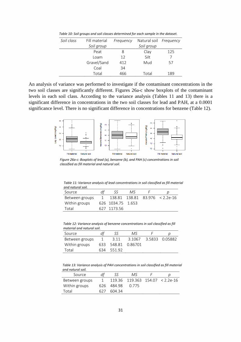
31

Table 10: Soil groups and soil classes determined for each sample in the dataset.

Table 11: Variance analysis of lead concentrations in soil classified as fill material and natural soil.

Figure 26a-c: Boxplots of lead (a), benzene (b), and PAH (c) concentrations in soil classified as fill material and natural soil.

Table 12: Variance analysis of benzene concentrations in soil classified as fill material and natural soil.

Table 13: Variance analysis of PAH concentrations in soil classified as fill material and natural soil.

Soil class Fill material Frequency Natural soil Frequency Soil group Soil group

Peat 8 Clay 125 Loam 12 Silt 7 Gravel/Sand 412 Mud 57 Coal 34

Total 466 Total 189

An analysis of variance was performed to investigate if the contaminant concentrations in the

two soil classes are significantly different. Figures 26a-c show boxplots of the contaminant

levels in each soil class. According to the variance analysis (Tables 11 and 13) there is a

significant difference in concentrations in the two soil classes for lead and PAH, at a 0.0001

significance level. There is no significant difference in concentrations for benzene (Table 12).

Source df SS MS F p

Between groups 1 138.81 138.81 83.976 < 2.2e-16 Within groups 626 1034.75 1.653

Total 627 1173.56

Source df SS MS F p

Between groups 1 3.11 3.1067 3.5833 0.05882 Within groups 633 548.81 0.86701

Total 634 551.92

Source df SS MS F p

Between groups 1 119.36 119.363 154.07 < 2.2e-16 Within groups 626 484.98 0.775

Total 627 604.34

32

Table 14: The parameters determined for lead, benzene and PAH from the geostatistical analysis.

Variation in spatial dependence in the two soil classes were investigated for lead and PAH. A

difference in the semi-variance in the two soil classes for both lead and PAH is detected

(Figures 27a-b). The sill value for lead concentrations in natural soil is about 0.6 and in fill

material about 2. The sill value for PAH concentrations in natural soil is about 0.6 and in fill

material about 0.8. That indicates that different semi-variance weights should be applied when

interpolating in the soil classes.

v) Summary

In the following interpolations residuals from the trend surface of the log transformed lead

concentrations are used. For benzene and PAH, the residuals of the normal score transformed

values are used.

No anisotropic relationship was found in the data, therefore no correction for 3D anisotropy

needs to be performed (Equation 2). A spatial dependence was found at short scales up to

about 2 m. The spatial dependence could only be seen in vertical directions. The shortest

sampling spacing in the horizontal plane is about 10 m. Therefore, the spatial dependence in

the horizontal plane shorter than 10 m is unknown.

There is a significant difference in concentrations in the upper fill material and the underlying

natural soil for lead and PAH. The semi-variance values vary in the two soil classes.

Therefore, the following interpolations of concentration levels in fill material and natural soil

for lead and PAH will be performed separately.

The final outcome of the geostatistical analysis and parameters used in the following

interpolations are presented in Table 14.

Lead (fill material)

Lead (natural soil)

Benzene PAH (fill material)

PAH (natural soil)

Model Spherical Spherical Spherical Spherical Spherical

Sill 1.81 0.6 0.66 0.84 0.6

Range 1.18 1.18 2.36 1.32 1.32

Nugget 0 0 0.31 0 0

Figure 27a-b: Variogram for lead (a) and PAH (b) in two different soil classes as well as semi-variance values for the whole dataset.

33

Table 15: The parameters used in the interpolations of lead concentrations.

b) 3D Interpolations

Considering computational complexity, sampling density and ranges a common 3D grid for

all interpolations and contaminants were decided. It was set to 5 x 5 m in the horizontal plane

and 0.20 m in the vertical plane. Other common parameters in the interpolations were the

minimum and maximum included samples. These were set to include at least 2 samples and

maximum 20 samples which is default in SADA. In Tables 15, 16 and 17 the final parameters

used in the interpolations for the three contaminants are summarized.

The interpolations of fill material and natural soil are separated by the mean depth of the fill

material. SADA cannot handle interpolations of a final volume with a varying depth. Points

deeper than the mean depth of the fill material (2.6 m) are interpolated with the parameters of

the natural soil. Points above 2.6 m are interpolated with parameters for the fill material.

The determined ranges for all three contaminants are shorter than the horizontal sampling

spacing. If these ranges were used as search radius in both horizontal and vertical plane there

would be no volume outcome. Therefore, different search radius was tested from the shortest

sampling spacing to the maximum separated distance between points. It was tested for three

different horizontal search radius; 10, 50, and 150 m. The final horizontal search radius for all

interpolations was the shortest radius (10 m), except from Kriging of benzene and lead in fill

material.

In the Kriging interpolations the discovered range, sill, and nugget parameters were used. The

length of the vertical search radius was set to the mean depth of the fill material and the

maximum depth of the natural soil. In the IDW interpolation the discovered ranges were used

as the vertical search radius length. For each of the search radius lengths three different

exponents (k) were tested as well; 1, 2, 3. The final exponent in the IDW interpolation

differed among the contaminants. An exponent of 2 was used for PAH interpolations, the

exponent 1 was used for benzene, as well as for lead in fill material. The exponent for lead in

natural soil was 2.

In the Nearest Neighbor interpolation three different vertical exaggerations were tested; no

exaggeration (1), double horizontal distance than vertical (10), and equal distance in

horizontal and vertical plane (20). The exaggeration did not affect the error validation since

the closets point was the same in all interpolations. The vertical exaggeration of 20 was used

in the final interpolations.

Lead Range Sill Horizontal

search radius Vertical

search radius Exponent Vertical

exaggeration

OK Fill material 1.18 1.81 150 2.6 - -

Natural soil 1.18 0.6 10 6 - - IDW

Fill material - - 10 1.18 1 - Natural soil - - 10 1.18 2 -

NN

Fill material - - - - - 20 Natural soil - - - - - 20

34

Table 16: The parameters used in the interpolations of benzene concentrations.

Table 17: The parameters used in the interpolations of PAH concentrations.

PAH Range Sill Horizontal

search radius Vertical

search radius Exponent Vertical

exaggeration

OK Fill material 1.32 0.84 10 2.6 - -

Natural soil 1.32 0.6 10 6 - - IDW

Fill material - - 10 1.32 2 - Natural soil - - 10 1.32 2 -

NN Fill material - - - - - 20

Natural soil - - - - - 20

i) Validation

The error validation with the validation dataset has an RMSE value for each interpolation. An

acceptable interpolation should have a low RMSE as close to 0 as possible. The RMSE values

depend on the data range in the original dataset. Therefore, the RMSE cannot be compared

among the contaminants.

The RMSE values from the predictions of lead shows that the Kriging interpolation and IDW

interpolation are equally good, and better than the Nearest Neighbor interpolation (Figure 28).

The difference in RMSE between Kriging and IDW when the interpolations in fill material

and natural soil are combined is negligible. The interpolations in the natural soil show the

least accurate result from the Kriging interpolation.

Benzene Range Sill Nugget Horizontal

search radius Vertical

search radius Exponent Vertical

exaggeration

OK 2.36 0.66 0.31 150 9 - - IDW - - - 10 2.36 1 - NN - - - - - - 20

Figure 28: The RMSE values for lead interpolations when compared to the validation dataset in the fill material, natural soil and total RMSE when the two are combined.

35

The RMSE values from the predictions of benzene shows a difference in accuracy among the

three interpolation methods (Figure 29). The most accurate interpolation method for benzene

is Kriging and the least accurate is the Nearest Neighbor interpolation.

The RMSE values from the predictions of PAH show the least difference in accuracy among

the interpolation methods (Figure 30). The interpolations in the fill material and the combined

interpolations show equal accuracy for all interpolations, although Kriging and IDW are

slightly better than the Nearest Neighbor interpolation. As for the lead interpolations in

natural soil, Kriging is the least accurate method for PAH in natural soil.

Figure 30: The RMSE values for PAH interpolations when compared to the validation dataset in the fill material, natural soil and total RMSE when the two are combined.

Figure 29: The RMSE values for benzene interpolations when compared to the validation dataset.

36

ii) Visualization and Implementation

In this section the final visualizations of the different interpolation methods are presented. The

figures show the combined interpolations in fill material and natural soil for lead and PAH.

The vertical dimension is exaggerated 5 times to enhance the vertical differences.

Lead

It is clear that the estimates of lead show enhanced levels from the surface and 2 m down in

the ground (Figure 31). At deeper levels no enhanced levels are estimated. It is due to few

samples and low concentrations in the original samples (Figure 17). The Kriging interpolation

is the method with largest effect of smoothing. The Nearest Neighbor interpolation does not

build on any geostatistics and interpolates the whole volume of natural soil (Figure 32). This

method also estimates a larger volume of high concentrations (Figure 33). The estimated

volume is just over 10,000 m3

for the Kriging and IDW interpolations. The least accurate

interpolation is Nearest Neighbor and estimates a contaminated soil volume of above 40,000

m3 (Figure 33).

Figure 31: The estimated mean concentrations of lead in 0.5 m depth intervals in the sampled volume for Kriging (OK), IDW and Nearest Neighbor (NN) interpolations. In the background the standard deviation of the original samples are shown.

Figure 32: Estimated volumes in percentage above risk

levels for lead interpolations in the sampled volume.

Figure 33: Estimated contaminated volumes above

risk levels for lead interpolations in the sampled

volume. Less sensitive land (400 mg/kg) and sensitive

land (50 mg/Kg)

37

The difference in level of smoothing between the interpolation methods for lead is also found

visually in Figure 34a-c. The few original samples at deeper levels in the natural soil results in

that no volume can be estimated in Kriging and IDW. All interpolations show similar areas of

highest concentrations.

Figure 35 shows the contaminated volume in 3D for the most accurate prediction, the Kriging

interpolation. It is only the upper soil layer close to the surface that shows contamination

levels above the risk level of lead. The major lead contamination does not exceed the risk

level of less sensitive land use nor sensitive land use.

Figure 34a-c: The results from the different interpolations of lead. The concentration classes are based on the limits in Table 3.

Figure 35: The soil volume estimated to be contaminated with lead according to the Kriging interpolation.

38

Benzene

Figure 36 shows that the IDW interpolation and Nearest Neighbor interpolation to a large

extent follow the distribution of the original samples of benzene concentrations. The Kriging

interpolation shows another pattern of lower mean values from the surface down to about 4 m

below the ground to increase further down in the soil volume. That shows the difference in a

geostatistical interpolation and deterministic.

The Kriging and Nearest Neighbor interpolations are able to estimate concentrations in larger

volumes than the IDW interpolation (Figure 37). The Kriging and Nearest Neighbor

interpolations also estimate larger contaminated volumes, from 160,000 m3 to almost 200,000

m3

(Figure 38). The IDW interpolation estimates the contaminated volume to less than 60,000

m3.

Figure 36: The estimated mean concentrations of benzene in 0.5 m depth intervals in the sampled volume for Kriging (OK), IDW and Nearest Neighbor (NN) interpolations. In the background the standard deviation of the original samples are shown.

Figure 38: Estimated contaminated volumes above

risk levels for benzene interpolations in the sampled

volume. Less sensitive land (0.012 mg/kg) and

sensitive land (0.04 mg/Kg)

Figure 37: Estimated volumes in percentage above risk

levels for benzene interpolations in the sampled volume.

39

All three interpolations show high benzene concentrations allocated around the old gasworks

(Figures 39a-c). There are also traces of contamination by the old dock. The Kriging

interpolation estimates high concentrations at deeper levels to a larger extent than can be seen

in the Nearest Neighbor interpolation. The IDW interpolation does not estimate the

concentrations at deeper levels.

Figure 40 shows the most accurate prediction of benzene contamination, the Kriging

interpolation. The prediction shows a large volume of high concentrations and a transportation

of benzene to deeper levels in the ground. The contamination is concentrated in close

proximity to the approximate locations of the old gasworks and dock. The contamination is

estimated to be spread further down in the volume and towards the river (South).

Figure 39a-c: The results from the different interpolations of benzene. The concentration classes are based on the limits in Table 3.

Figure 40: The soil volume estimated to be contaminated with benzene according to the Kriging interpolation.

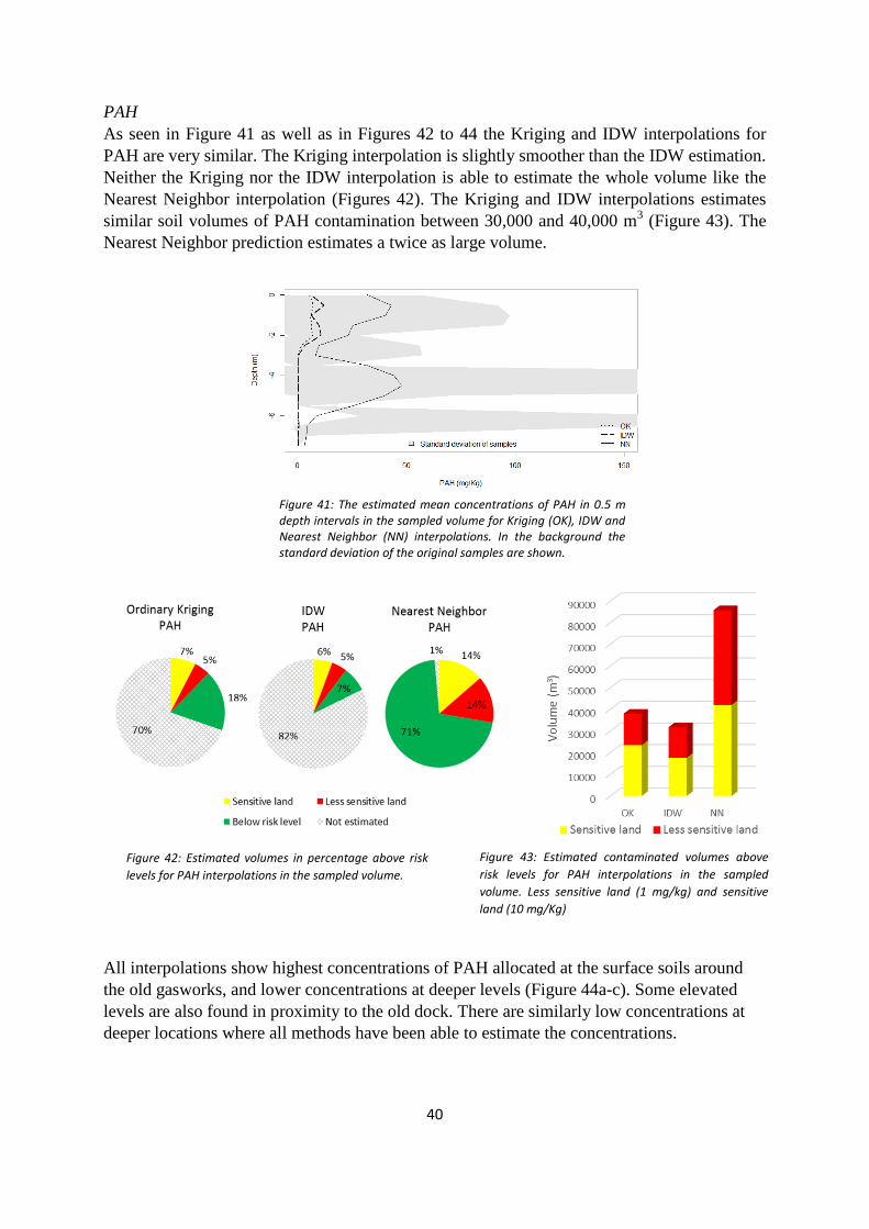
40

PAH

As seen in Figure 41 as well as in Figures 42 to 44 the Kriging and IDW interpolations for

PAH are very similar. The Kriging interpolation is slightly smoother than the IDW estimation.

Neither the Kriging nor the IDW interpolation is able to estimate the whole volume like the

Nearest Neighbor interpolation (Figures 42). The Kriging and IDW interpolations estimates

similar soil volumes of PAH contamination between 30,000 and 40,000 m3 (Figure 43). The

Nearest Neighbor prediction estimates a twice as large volume.

All interpolations show highest concentrations of PAH allocated at the surface soils around

the old gasworks, and lower concentrations at deeper levels (Figure 44a-c). Some elevated

levels are also found in proximity to the old dock. There are similarly low concentrations at

deeper locations where all methods have been able to estimate the concentrations.

Figure 41: The estimated mean concentrations of PAH in 0.5 m depth intervals in the sampled volume for Kriging (OK), IDW and Nearest Neighbor (NN) interpolations. In the background the standard deviation of the original samples are shown.

Figure 43: Estimated contaminated volumes above

risk levels for PAH interpolations in the sampled

volume. Less sensitive land (1 mg/kg) and sensitive

land (10 mg/Kg)

Figure 42: Estimated volumes in percentage above risk

levels for PAH interpolations in the sampled volume.

41

Figure 45 shows the most accurate prediction of PAH contamination, the Kriging

interpolation. The prediction of PAH concentrations above the risk level for less sensitive

land are in the upper layer of the soil in close proximity to the gasworks. The concentrations

decrease to above the risk level for sensitive land at deeper locations and at the old dock.

Figure 44a-c: The results from the different interpolations of PAH. The concentration classes are based on the limits in Table 3.

Figure 45: The soil volume estimated to be contaminated with PAH according to the Kriging interpolation.

42

5. Discussion

a) Evaluation of 3D Interpolation Models

Three different interpolation methods have been compared; Kriging, IDW, and Nearest

Neighbor. The parameters of the Kriging and IDW interpolations were optimized using the

results from geostatistical analyses and validations while the Nearest Neighbor does not allow

for such optimization.

All three interpolation methods detected the assumed locations of the former gasworks as

areas of high risk levels. The Nearest Neighbor method was able to estimate the whole

volume of the study area. Yet it was the least accurate, and if the predicted volume is

inaccurate it will not help the evaluation of remediation measures. From the RMSE values

(Figure 28-30) and since a spatial relation was found, the best method of the evaluated ones

are Kriging and secondly the IDW interpolation for all contaminants. Both are based on the

parameters from the geostatistical analyses. A similar 3D evaluation of the three methods on

lead contamination was performed by Wei et al. (2014). They also found that Kriging was the

most accurate method. This is also in line with previous studies on soil contamination data in

2D (Xie et al., 2011).

The findings emphasize the importance of a geostatistical analysis before a useful

interpolation can be performed. In most cases the Kriging and IDW methods are able to

estimate around 25% of the volume in the study area (Figure 34a, 39a, 44a). That means that

the interpolations will help to size up a picture of the contamination situation, especially

compared to a situation where the actual sampling points are the only available information.

The evaluated interpolations were restricted to the available methods in one software.

Therefore, spline interpolation for example was not evaluated. Some studies suggest that the

spline method RST is the optimal interpolation method. One example is the study of Piedade

et al. (2014) that evaluated the RST method in three dimensions for lead with a satisfying

result. According to Mitáš & Mitášová (1999) RST is the easiest and best interpolation

method to use for unexperienced users.

b) Evaluation on Contaminant Differences

Contaminants with different characteristics were studied. From the analyses, their different

characteristics induced varying parameters and methods for interpolation. Benzene was

distinguished from the other two contaminants having a larger spatial dependence and being

spread into the natural soil. This is in line with the characteristics of benzene being a

lightweight pollutant easily traveling with the groundwater (Table 1). The benzene

interpolations were also the ones with the greatest potential of a valid prediction model. The

differences in RMSE among the studied interpolation methods were greatest for benzene

compared to the other two contaminants. It gives a clear indication on that Kriging

interpolation is a good method for modeling soil contaminants that easily transports down into

the ground.

The analyses of lead and PAH showed more similarities than differences. That is presumably

due to their similar characteristics of being persistent in the environment and too large for

transportation downwards (Table 1). Their persistence is also detected in their short ranges

determining the spatial dependence (Table 14). The results show that Kriging and IDW

interpolations give equal results for these types of contaminants. Lead has the highest sill of

43

the three contaminants. The high sill emphasizes the inability of lead to be distributed in the

ground resulting in a large variability of high and low concentrations. The estimated

contamination of lead is low (below the level of less sensitive land) and concentrated at the

surface (Figure 45). According to Steinnes (2013) high concentrations of lead are necessary

for transportation downwards indicating that the result is valid.

The results of the analyses show that PAH is not spread extensively in the natural soil. The fill

material consists of more organic soils than natural (Table 10). A high organic content is

important for transportation of PAH (Abdel-Shafy & Mansour, 2016). Therefore, it is

reasonable to believe that the estimated contamination levels at deeper locations in the natural

soil are valid.

According to the RMSE values the interpolation results of PAH might be questioned. The

standard variation of the PAH samples (Table 7) is smaller than the RMSE values (Figure 30).

That means that the variation of PAH might not be captured in the interpolation. The standard

variation of the benzene samples are a lot larger than the RMSE values from both Kriging and

IDW, the same goes for lead. Lead and benzene are both on the extremes, lead is a very

persistent contaminant and benzene a very volatile one. PAH however, is more intermediate.

PAH is persistent but not to the same extent as lead. Noticeably, it is more difficult to predict

the distribution of a more varying contaminant (Xie et al., 2011).

The lower concentrations of lead and PAH in the natural soil (Figure 26a and c) suggests that

the contaminants have not been transported to a large extent to the natural soil. Therefore,

samples in the natural soil could be excluded to speed up the process when these are

interpolated.

c) Evaluation on Methods for 3D Interpolation with GIS

To keep the contamination data within a GIS-environment increases the possibilities for

further analyses. Compared to a 3D modeling software a GIS keeps the spatial attributes and

relationships. Information that is important for remediation decisions and other conclusions

that should be drawn from the data.

The ultimate solution for a project with risk assessment of soil contamination would be to

work within the GIS-environment from start to end with planning, sampling, analysis and

describing the situation, to the remediation measure. That could give a more effective work

process as well as ease the work for people with less GIS- and computer skills. In ArcGIS, as

Sweco use, many of these steps are possible today. With further work of the suggested

prototype for 3D interpolation (Figures 7-8) the possibility exists to perform 3D interpolation

in ArcGIS. In reality, this is not an optimal solution. The optimal solution has a wide range of

interpolation techniques to choose from since different sampling densities and contaminants

might need different approaches. Instead the technique of integrating 3D volumes in GISs

needs to be further developed before a complete work process including 3D interpolation

within a GIS is feasible in a comprehensive way.

GRASS GIS was suggested as software for 3D interpolation that is both a GIS and can handle

3D volumes. The study of Neteler (2001) suggests that the methods in GRASS are good for

volume interpolation of soil contaminants with the strength of seamless integration into a GIS.

However, GRASS lacks the streamlined approach from sampling to visualization. These are

important qualities in a method suitable for larger projects for contaminated sites. The largest

44

downside with GRASS is the lacking possibility of Kriging interpolation suggested to be the

most accurate method. Programming and additional open source alternatives might be useful

to overcome these issues and still use GRASS.

MVS and other 3D modeling software are certainly alternatives for robust and reliable 3D

models. The downside is the high license cost that might not increase the final outcome of the

remediation measure distinctly from more simple software. Furthermore, these are not

incorporated in any GIS and need time consuming data processing before performance. They

also need a certain skill of data processing to be used. On the positive side, MVS performs the

geostatistical analyses with optimal solutions in an automatic way. SADA is free but has the

same problem with data processing as other more sophisticated 3D software. However, the

interface of SADA is easy to use and ordered in a logic manner for both beginners and experts

in data processing. In SADA geostatistical analysis can be performed within the user interface

giving the user more control on the final outcome. Although compared to MVS that can

perform optimal interpolations without integration from the user, geoscientific knowledge is

needed in SADA.

According to Mitáš & Mitášová (1999) methods have been presented which are capable of

treatment of multi-dimensional data. However, the current GIS computational infrastructure

does not effectively support a wide application of multi-dimensional modeling. This seems to

be valid today as well. Until the technique is further developed or other methods exists the

proposed method for 3D interpolation is to perform the geostatistical analysis and

interpolations in another software, as SADA or MVS, and then transfer the data back into a

GIS again to make use of the pros a GIS comes with. The method for geostatistical analyses

and interpolation performed in this study is too complex for a general contamination project

since too many software is involved.

d) Reliability of the Results and Future Research

The results suggest that soil contamination prediction in 3D is possible to different extents

and certain degree of reliability. However, the sampling density in the horizontal plane is too

coarse to find any spatial dependence. Or possibly, the study area is too small to detect the

spatial dependence. That makes the result more unreliable than if a clear spatial dependence

was found also in the horizontal plane. Although, one might suggests, as in the study, that the

relationship is isotropic and the spatial dependence very small. That means a fine layering and

grid spacing must be used to interpolate in 3D. Consequently, that increases the computational

complexity especially working within a GIS where each grid point is stored as a separate unit.

All parameters in the interpolations have not been optimized. Grid size and included samples

are examples of non-optimized parameters. However, the sampling density does not allow for

a finer grid. There is a possibility that the number of included samples for each estimated

point could have an effect on the results. It is something that could have been further studied

in future research. Furthermore, since no spatial dependence was found in the horizontal plane

three different lengths of search radius were tested for Kriging and IDW interpolations. The

optimal search radiuses of these three were used, although it can still be another search radius

with another length not investigated that is more suitable.

Another weakness of the study is the interpolations at deeper levels. Firstly, the numbers of

samples in natural soil at levels deeper than about 2.5 m are less than half of the samples in

the fill material. Still, the natural soil is interpolated as a separate part although the samples

might be too few for interpolation.

45

Secondly, the division in natural soil and fill material is performed on the mean depth of the

fill material. Since the depth in reality is varying, samples in fill material has been

interpolated with natural soil parameters and vice versa. This is a limitation in the software

used which might be solvable in more solid 3D modeling software. For more reliable results

more samples at deeper levels are necessary as well as a higher sampling density in the

horizontal plane.

An additional suggestion for future research is to compare the 3D volume interpolations with

2D interpolations at surfaces on different depths. If the result is similar, that would mean an

easier interpolation approach where the whole process can be performed in a GIS.

The back transformation of logarithmic transformed with exponentiation might exaggerate the

data values (Goovaerts, 1997). The exaggeration affect can in the future be mitigated with the

use of an unbiased back transformation (Deutsch & Journel, 1998). Also, the normal score

transformation of the data can have an effect on the result. In this case, the back

transformation was set to keeping the original minimum and maximum from the samples in

the interpolated values. However, it is the exceeding of the two risk levels that is important in

projects for contaminated land. Small differences as transformation errors would not affect the

final outcome of the risk levels.

The results in the study are validated with RMSE values from another sampling dataset. That

means that these samples are not located at the same spot as the interpolated points. The

distribution of the validation points might also have an effect. The outcomes of the

interpolations had volumes not estimated. That means that a varying numbers of validation

points were included in the validation. Also, to state with confidence which method that is the

best, even more types of validations are desirable.

All in all, every model is just an estimate about the real world situation. There is not only one

model that can describe the whole reality. Finally, the approach is based on the assumption

that the samples used are representative in themselves, this is not always true (Houlding,

2000).

6. Conclusion

Volume interpolation of soil pollutants has a high potential to add knowledge and insight into

the contamination situation at a site. The interpolations performed here were able to detect

differences regarding the distribution patterns of the three contaminants. Estimates of volumes

above risk levels could be computed, areas of high risk have been detected as well as the

transportation down in the ground. However, no spatial dependence in the horizontal plane

was found making the results more unreliable. A higher sampling density is necessary for a

more solid result.

Lead, benzene, and PAH all show the greatest potential of interpolation with Kriging.

Nevertheless, for lead and PAH the IDW interpolations show similar potentials. The different

characteristics of the three contaminants resulted in different optimal parameters for the

interpolations. A major detected difference was the distribution in the ground which was

notable for benzene but not for the other two contaminants. Mobile contaminants as benzene

should be interpolated with different parameters than the more immobile contaminants lead

and PAH.

46

Benzene showed the greatest potential of interpolating 3D volumes. It had a high accuracy

and the whole volume in the study area could be interpolated. Lead showed a good potential

of interpolating in the fill material of the soil. For a reliable interpolation in the natural soil

more samples are needed. PAH showed the least potential of volume interpolation with a low

accuracy of the interpolation and only parts of the whole volume of the study area could be

interpolated.

Based on the results a complete, accurate and effective interpolation of 3D volumes is today

difficult to perform in a GIS-environment alone. It is therefore suggested to combine the work

with contamination data in a GIS with more solid 3D modeling. The geostatistical analysis is

an important part in the interpolation since the method not based on geostatistics was least

accurate. Geostatistical analysis of 3D data is difficult to perform within a GIS and additional

software is needed. The effectiveness is higher in software as MVS which optimize the

parameters within the software while software as SADA gives more control to the user.

A three dimensional visualization of the contamination may increase the understanding and

increase the foundation for remediation measures. Nevertheless, one must be aware of that it

is a model and not the real situation.

47

7. References

Abdel-Shafy, H. I., & Mansour, M. S. (2016). A review on polycyclic aromatic hydrocarbons: source,

environmental impact, effect on human health and remediation. Egyptian Journal of Petroleum, 25(1),

107-123.

Abdul-Rahman, A., & Pilouk, M. (2008). Spatial data modelling for 3D GIS. Berlin: Springer Science &

Business Media.

Agency for Toxic Substances and Disease Registry (ATSDR). 1995. Toxicological profile for Polycyclic

Aromatic Hydrocarbons (PAHs). Atlanta, GA: U.S. Department of Health and Human Services, Public

Health Service.

Agency for Toxic Substances and Disease Registry (ATSDR). 2007a. Toxicological profile for Benzene.

Atlanta, GA: U.S. Department of Health and Human Services, Public Health Service.

Agency for Toxic Substances and Disease Registry (ATSDR). 2007. Toxicological profile for Lead. Atlanta,

GA: U.S. Department of Health and Human Services, Public Health Service.

ArcGIS. [Computer software] http://www.arcgis.com/

ArcGIS Online. http://www.arcgisonline.com/

Bohling, G. (2005). Introduction to geostatistics and variogram analysis. Kansas geological survey, 20p.

Brandon, E. (2013). The Nature and Extent of Site Contamination. In Global Approaches to Site Contamination

Law (pp. 11-39). Dordrecth: Springer Science & Business Media.

Cairns, J. L., & Feldkamp, L. D. (1993). 3D visualization for improved reservoir characterization. SPE

Computer Applications, 5(03), 13-24.

Carlon, C., Hope, B., & Quercia, F. (2009). Contaminated land: a multi-dimensional problem. In Marcomini, A.,

Suter, G. W., & Critto, A. (Eds.). Decision Support Systems for Risk-Based Management of Contaminated

Sites (pp. 1-23). New York: Springer Science & Business Media.

Chambers, J., Ogilvy, R., Meldrum, P., & Nissen, J. (1999). 3D resistivity imaging of buried oil- and tar-

contaminated waste deposits. European Journal of Environmental and Engineering Geophysics, 4(1), 3-

14.

C’tech. (2015). EVS/MVS Help Version 9.94. http://www.ctech.com/

Deutsch, C.V., & Journel, A.G. (1998). GSLIB, Geostatistical Software Library and User’s Guide. New York:

Oxford University Press.

Fent, K. (2004). Ecotoxicological effects at contaminated sites. Toxicology, 205(3), 223-240.

Goovaerts, P. Geostatistical software. (2009). In Fischer, M. M., & Getis, A. (Eds.) Handbook of applied spatial

analysis: software tools, methods and applications. Springer Science & Business Media.

Goovaerts, P. (1997). Geostatistics for natural resources evaluation. New York: Oxford University Press.

GRASS GIS. [Computer software] https://grass.osgeo.org/

Hengl, T. (2007). A practical guide to geostatistical mapping. EUR 22904 EN. Luxembourg: Office for Official

Publications of the European Communities.

Henriksson, S., Hagberg, J., Bäckström, M., Persson, I., & Lindström, G. (2013). Assessment of PCDD/Fs levels

in soil at a contaminated sawmill site in Sweden–A GIS and PCA approach to interpret the contamination

pattern and distribution. Environmental pollution, 180, 19-26.

48

Henshaw, S. L., Curriero, F. C., Shields, T. M., Glass, G. E., Strickland, P. T., & Breysse, P. N. (2004).

Geostatistics and GIS: tools for characterizing environmental contamination. Journal of medical systems,

28(4), 335-348.

Houlding, S. (2000). Practical geostatistics: modeling and spatial analysis. Berlin: Springer Science & Business

Media.

Houlding, S. (2012). 3D geoscience modeling: computer techniques for geological characterization. Berlin:

Springer Science & Business Media.

Isaaks, E. H., & Srivastava, R. M. (1989). Applied geostatistics. New York: Oxford University Press.

Juang, K. W., Lee, D. Y., & Ellsworth, T. R. (2001). Using rank-order geostatistics for spatial interpolation of

highly skewed data in a heavy-metal contaminated site. Journal of Environmental Quality, 30(3), 894-

903.

Largueche, F. Z. B. (2006). Estimating soil contamination with Kriging interpolation method. American Journal

of Applied Sciences, 3(6), 1894-1898.

Luthy, R. G., Dzombak, D. A., Peters, C. A., Roy, S. B., Ramaswami, A., Nakles, D. V., & Nott, B. R. (1994).

Remediating tar-contaminated soils at manufactured gas plant sites. Environmental Science &

Technology, 28(6), 266A-276A.

Mallet, J. L., Jacquemin, P., & Cheimanoff, N. (1989). GOCAD project: Geometric modeling of complex

geological surfaces. In 1989 SEG Annual Meeting. Society of Exploration Geophysicists.

Mallet, J. L. (1992). GOCAD: a computer aided design program for geological applications. In Three-

dimensional modeling with geoscientific information systems (pp. 123-141). Dordrecth: Springer Science

& Business Media.

Manto, H. (2005). Modelling of geometric anisotropic spatial variation. Mathematical Modelling and Analysis,

361-366.

Matheron, G. (1963). Principles of geostatistics. Economic geology, 58(8), 1246-1266.

Matheron, G. (1971). The theory of regionalized variables and its applications (Vol. 5, p. 211pp). École national

supérieure des mines.

McCarthy, J. D., & Graniero, P. A. (2006). A GIS-based borehole data management and 3D visualization

system. Computers & Geosciences, 32(10), 1699-1708.

Mirsal, I. A. (2008). Soil Pollution. Origin, Monitoring & Remediation. Berlin: Springer Science & Business

Media.

Mitáš, L., & Mitášová, H. (1999). Spatial interpolation. Geographical information systems: principles,

techniques, management and applications, 1, 481-492.

Mitášová, H., & Mitáš, L. (1993). Interpolation by regularized spline with tension: I. Theory and

implementation. Mathematical geology, 25(6), 641-655.

MVS. [Computer software] http://www.ctech.com/

Naturvårdsverket. (2016). Lägesbeskrivning av arbetet med efterbehandling av förorenade områden 2015.

Stockholm: Naturvårdsverkets förlag.

Naturvårdsverket. (2009a). Riskbedömning av förorenade områden. En vägledning från förenklad till fördjupad

riskbedömning. Stockholm: Naturvårdsverkets förlag.

Naturvårdsverket. (2009b). Riktvärden för förorenad mark. Modellbeskrivning och vägledning. Stockholm:

Naturvårdsverkets förlag.

49

Neteler, M. Volume modeling of soils using GRASS GIS 3D-Tools. (2001). In Brovelli, M. (Ed.). The geomatics

workbook 2 (2001). Politecnico di Milano.

Nichol, J. E., Wong, M. S., & Wang, J. (2010). A 3D aerosol and visibility information system for urban areas

using remote sensing and GIS. Atmospheric Environment, 44(21), 2501-2506.

Oliver, M. A. The variogram and Kriging. (2009). In Fischer, M. M., & Getis, A. (Eds.) Handbook of applied

spatial analysis: software tools, methods and applications. Springer Science & Business Media.

Panagos, P., Van Liedekerke, M., Yigini, Y., & Montanarella, L. (2013). Contaminated sites in Europe: review

of the current situation based on data collected through a European network. Journal of environmental

and public health, 2013.

Pebesma, E.J., 2004. Multivariable geostatistics in S: the gstat package. Computers & Geosciences, 30: 683-691.

Piedade, T. C., Souza, L. C. P., & Dieckow, J. (2014). Three-dimensional data interpolation for environmental

purpose: lead in contaminated soils in southern Brazil. Environmental monitoring and assessment, 186(9),

5625-5638.

Prokop, G., Schamann, M., Edelgaard I. (2000). Management of contaminated sites in Western Europe.

Copenhagen: European Environmental Agency.

Purucker, S. T., Stewart, R. N., & Welsh, C. J. (2009). SADA: ecological risk based decision support system for

selective remediation. In Marcomini, A., Suter, G. W., & Critto, A. (Eds.). Decision Support Systems for

Risk-Based Management of Contaminated Sites (pp. 1-18). New York: Springer Science & Business

Media.

R Core Team (2016). R: A language and environment for statistical computing. R Foundation for Statistical

Computing, Vienna, Austria. https://www.R-project.org/

Ranga Vital, T., Trpathy, G.K., & Mishra, B. (2015). A GIS-borehole data management and 3D visualization

system: a case study of Pitisal sand deposit along Puri Coast, Odisha, India. Journal of Coastal Sciences,

2(1).

RStudio Team .(2015). RStudio: Integrated Development for R. RStudio, Inc., Boston, MA.

http://www.rstudio.com/

SADA. [Computer software] http://www.sadaproject.net/

SADA. (2005). V5 SADA User guide. http://www.sadaproject.net/

Setijadji, D.L. (2003). GIS for subsurface modeling. Prepared for ESRI Book Publication entitled: Subsurface

Modeling With GIS.

Shepard, D. (1968). A two-dimensional interpolation function for irregularly-spaced data. In Proceedings of the

1968 23rd ACM national conference (pp. 517-524). ACM.

Steinnes, E. (2013). Lead. In Alloway, B. J. (Ed.), Heavy metals in soils: trace metals and metalloids in soils and

their bioavailability (pp. 395-409). Dordrecth: Springer Science & Business Media.

Swartjes, F. A. (2011). Introduction to contaminated site management. In Dealing with contaminated sites (pp.

3-89). Dordrecth: Springer Science & Business Media.

Sweco .(2015). Huvudstudie omfattande gasverksområdet (fastigheterna Skeppsdockan 1, 3, 5 samt del av

Saltängen 1:1) i Norrköpings kommun.

Tobler, W. R. (1970). A computer movie simulating urban growth in the Detroit region. Economic geography,

46, 234-240.

Warfvinge, P. (1997). Miljökemi: miljövetenskap i biogeokemiska perspektiv. Lund: KFS.

50

Wei, W. X., Quan, T., Wang, Y., Wang, H. J., & Li, P. Z. (2014). Application of Three-dimensional

Interpolation Methods in Contaminated Site Evaluation. Advanced Materials Research, 878, 782-790.

Wuana, R. A., & Okieimen, F. E. (2011). Heavy metals in contaminated soils: a review of sources, chemistry,

risks and best available strategies for remediation. ISRN Ecology, 2011.

Xie, Y., Chen, T. B., Lei, M., Yang, J., Guo, Q. J., Song, B., & Zhou, X. Y. (2011). Spatial distribution of soil

heavy metal pollution estimated by different interpolation methods: accuracy and uncertainty analysis.

Chemosphere, 82(3), 468-476.

Xikui, L., Yongfa, L., & Peipei, S. (2016). Study on Three Dimensional Modeling and Visualization in Geology.

The Open Civil Engineering Journal, 10(1).

Zahran, E. S. M., Smith, M. J., & Bennett, L. D. (2012). 3D visualization of traffic-induced air pollution impacts

of urban transport schemes. Journal of Computing in Civil Engineering, 27(5), 452-465.

51

Institutionen för naturgeografi och ekosystemvetenskap, Lunds Universitet.

Student examensarbete (Seminarieuppsatser). Uppsatserna finns tillgängliga på institutionens

geobibliotek, Sölvegatan 12, 223 62 LUND. Serien startade 1985. Hela listan och själva uppsatserna är

även tillgängliga på LUP student papers (https://lup.lub.lu.se/student-papers/search/) och via

Geobiblioteket (www.geobib.lu.se)

The student thesis reports are available at the Geo-Library, Department of Physical Geography and Ecosystem Science, University of Lund, Sölvegatan 12, S-223 62 Lund, Sweden. Report series started 1985. The complete list and electronic versions are also electronic available at the LUP student papers (https://lup.lub.lu.se/student-papers/search/) and through the Geo-library (www.geobib.lu.se)

350 Mihaela – Mariana Tudoran (2015) Occurrences of insect outbreaks in Sweden in

relation to climatic parameters since 1850

351 Maria Gatzouras (2015) Assessment of trampling impact in Icelandic natural areas in

experimental plots with focus on image analysis of digital photographs

352 Gustav Wallner (2015) Estimating and evaluating GPP in the Sahel using MSG/SEVIRI

and MODIS satellite data

353 Luisa Teixeira (2015) Exploring the relationships between biodiversity and benthic

habitat in the Primeiras and Segundas Protected Area, Mozambique

354 Iris Behrens & Linn Gardell (2015) Water quality in Apac-, Mbale- & Lira district,

Uganda - A field study evaluating problems and suitable solutions

355 Viktoria Björklund (2015) Water quality in rivers affected by urbanization: A Case

Study in Minas Gerais, Brazil

356 Tara Mellquist (2015) Hållbar dagvattenhantering i Stockholms stad - En

riskhanteringsanalys med avseende på långsiktig hållbarhet av Stockholms stads

dagvattenhantering i urban miljö

357 Jenny Hansson (2015) Trafikrelaterade luftföroreningar vid förskolor – En studie om

kvävedioxidhalter vid förskolor i Malmö

358 Laura Reinelt (2015) Modelling vegetation dynamics and carbon fluxes in a high

Arctic mire

359 Emelie Linnéa Graham (2015) Atmospheric reactivity of cyclic ethers of relevance to

biofuel combustion

360 Filippo Gualla (2015) Sun position and PV panels: a model to determine the best

orientation

361 Joakim Lindberg (2015) Locating potential flood areas in an urban environment using

remote sensing and GIS, case study Lund, Sweden

362 Georgios-Konstantinos Lagkas (2015) Analysis of NDVI variation and snowmelt

around Zackenberg station, Greenland with comparison of ground data and remote

sensing.

363 Carlos Arellano (2015) Production and Biodegradability of Dissolved Organic Carbon

from Different Litter Sources

364 Sofia Valentin (2015) Do-It-Yourself Helium Balloon Aerial Photography - Developing

a method in an agroforestry plantation, Lao PDR

365 Shirin Danehpash (2015) Evaluation of Standards and Techniques for Retrieval of

Geospatial Raster Data - A study for the ICOS Carbon Portal

52

366 Linnea Jonsson (2015) Evaluation of pixel based and object based classification

methods for land cover mapping with high spatial resolution satellite imagery, in the

Amazonas, Brazil.

367 Johan Westin (2015) Quantification of a continuous-cover forest in Sweden using

remote sensing techniques

368 Dahlia Mudzaffar Ali (2015) Quantifying Terrain Factor Using GIS Applications for

Real Estate Property Valuation

369 Ulrika Belsing (2015) The survival of moth larvae feeding on different plant species in

northern Fennoscandia

370 Isabella Grönfeldt (2015) Snow and sea ice temperature profiles from satellite data

and ice mass balance buoys

371 Karolina D. Pantazatou (2015) Issues of Geographic Context Variable Calculation

Methods applied at different Geographic Levels in Spatial Historical Demographic

Research -A case study over four parishes in Southern Sweden

372 Andreas Dahlbom (2016) The impact of permafrost degradation on methane fluxes -

a field study in Abisko

373 Hanna Modin (2016) Higher temperatures increase nutrient availability in the High

Arctic, causing elevated competitive pressure and a decline in Papaver radicatum

374 Elsa Lindevall (2016) Assessment of the relationship between the Photochemical

Reflectance Index and Light Use Efficiency: A study of its seasonal and diurnal

variation in a sub-arctic birch forest, Abisko, Sweden

375 Henrik Hagelin and Matthieu Cluzel (2016) Applying FARSITE and Prometheus on the

Västmanland Fire, Sweden (2014): Fire Growth Simulation as a Measure Against

Forest Fire Spread – A Model Suitability Study –

376 Pontus Cederholm (2016) Californian Drought: The Processes and Factors Controlling

the 2011-2016 Drought and Winter Precipitation in California

377 Johannes Loer (2016) Modelling nitrogen balance in two Southern Swedish spruce

plantations

378 Hanna Angel (2016) Water and carbon footprints of mining and producing Cu, Mg

and Zn: A comparative study of primary and secondary sources

379 Gusten Brodin (2016) Organic farming’s role in adaptation to and mitigation of

climate change - an overview of ecological resilience and a model case

study

380 Verånika Trollblad (2016) Odling av Cucumis Sativus L. med aska från träd som

näringstillägg i ett urinbaserat hydroponiskt system

381 Susanne De Bourg (2016) Tillväxteffekter för andra generationens granskog efter

tidigare genomförd kalkning

382 Katarina Crafoord (2016) Placering av energiskog i Sverige - en GIS analys

383 Simon Nåfält (2016) Assessing avalanche risk by terrain analysis An experimental GIS-approach to The Avalanche Terrain Exposure Scale (ATES)

384 Vide Hellgren (2016) Asteroid Mining - A Review of Methods and Aspects

385 Tina Truedsson (2016) Hur påverkar snömängd och vindförhållande

vattentrycksmätningar vintertid i en sjö på västra Grönland?

386 Chloe Näslund (2016) Prompt Pediatric Care Pediatric patients’ estimated travel

times to surgically-equipped hospitals in Sweden’s Scania County

387 Yufei Wei (2016) Developing a web-based system to visualize vegetation trends by a nonlinear regression algorithm

53

388 Greta Wistrand (2016) Investigating the potential of object-based image analysis to

identify tree avenues in high resolution aerial imagery and lidar data

389 Jessica Ahlgren (2016) Development of a Web Mapping Application for grazing

resource information in Kordofan, Sudan, by downloading MODIS data automatically

via Python

390 Hanna Axén (2016) Methane flux measurements with low-cost solid state sensors in

Kobbefjord, West Greenland

391 Ludvig Forslund (2016) Development of methods for flood analysis and response in a

Web-GIS for disaster management

392 Shuzhi Dong (2016) Comparisons between different multi-criteria decision analysis

techniques for disease susceptibility mapping

393 Thirze Hermans (2016) Modelling grain surplus/deficit in Cameroon for 2030

394 Stefanos Georganos (2016) Exploring the spatial relationship between NDVI and

rainfall in the semi-arid Sahel using geographically weighted regression

395 Julia Kelly (2016) Physiological responses to drought in healthy and stressed trees: a

comparison of four species in Oregon, USA

396 Antonín Kusbach (2016) Analysis of Arctic peak-season carbon flux estimations based

on four MODIS vegetation products

397 Luana Andreea Simion (2016) Conservation assessments of Văcărești urban wetland

in Bucharest (Romania): Land cover and climate changes from 2000 to 2015

398 Elsa Nordén (2016) Comparison between three landscape analysis tools to aid

conservation efforts

399 Tudor Buhalău (2016) Detecting clear-cut deforestation using Landsat data: A time

series analysis of remote sensing data in Covasna County, Romania between 2005

and 2015

400 Sofia Sjögren (2016) Effective methods for prediction and visualization of

contaminated soil volumes in 3D with GIS