1

Effective Sampling: Fast Segmentation UsingRobust Geometric Model Fitting

Ruwan Tennakoon, Alireza Sadri, Reza Hoseinnezhad, and Alireza Bab-Hadiashar, Senior Member, IEEE

Abstract—Identifying the underlying models in a set of datapoints contaminated by noise and outliers, leads to a highlycomplex multi-model fitting problem. This problem can be posedas a clustering problem by the projection of higher order affinitiesbetween data points into a graph, which can then be clusteredusing spectral clustering. Calculating all possible higher orderaffinities is computationally expensive. Hence in most casesonly a subset is used. In this paper, we propose an effectivesampling method to obtain a highly accurate approximation ofthe full graph required to solve multi-structural model fittingproblems in computer vision. The proposed method is based onthe observation that the usefulness of a graph for segmentationimproves as the distribution of hypotheses (used to build thegraph) approaches the distribution of actual parameters forthe given data. In this paper, we approximate this actualparameter distribution using a k-th order statistics based costfunction and the samples are generated using a greedy algorithmcoupled with a data sub-sampling strategy. The experimentalanalysis shows that the proposed method is both accurate andcomputationally efficient compared to the state-of-the-art robustmulti-model fitting techniques. The code is publicly availablefrom https://github.com/RuwanT/model-fitting-cbs.

Index Terms—Model-fitting , Spectral clustering , Data seg-mentation , motion segmentation , Hyper-graph

I. INTRODUCTION

Robust fitting of geometric models to data contaminatedwith both noise and outliers is a well studied problem withmany applications in computer vision [1, 2, 3, 4]. Visualdata often contain multiple underlying structures and there arepseudo-outliers (measurements representing structured otherthan the structure of interest [5]) as well as gross-outliers(produced by errors in the data generation process). Fittingmodels to this combination of data involves solving a highlycomplex multi-model fitting problem. The above multi-modelfitting problem can be viewed as a combination of twosub problems: data labeling and model estimation. Althoughsolving one of the sub-problems, when the solution to the otheris given, is straightforward, solving both problems simultane-ously remains a challenge.

Traditional approaches to multi-model fitting were basedon fit and remove strategy: apply a high breakdown robustestimator (e.g. RANSAC [1], least k-th order residual) togenerate a model estimate and remove its inliers to preventthe estimator from converging to the same structure again.However, this approach is not optimal as errors made in theinitial stages tend to make the subsequent steps unreliable (e.g.small structures can be absorbed by models that are createdby accidental alignment of outliers with several structures)[6]. To address this issue, energy minimization methods havebeen proposed. They are based on optimizing a cost func-

R.B. Tennakoon, A. Sadri, R. Hoseinnezhad and A. Bab-Hadiashar are withthe School of Engineering, RMIT University, Melbourne, Australia.E-mail: ruwan.tennakoon@rmit.edu.au

tion consisting of a combination of data fidelity and modelcomplexity (number of model instances) terms [7]. In thisapproach, the cost function is optimized to simultaneouslyrecover the number of structures and their data association.Commonly such cost functions are optimized using discreteoptimization methods (metric labeling [2]). They start form alarge number of proposal hypotheses and gradually convergeto the true models. The outcome of those methods dependson the appropriate balance between the two terms in the costfunction (controlled by an input parameter) as well as thequality of initial hypotheses. The method proposed in thispaper is primarily designed to avoid the use of parameters thatare difficult to tune. Sensitivity to the parameters included forthe summation of terms with different dimensions is also anissue associated with the application of several other subspacelearning and clustering methods. For instance, Robust-PCA[8] splits the data matrix into a low-rank matrix and a sparseerror matrix. The aim is to minimize the cost function (whichis a norm of the error matrix) while it is regularized by arank of representation matrix. In factorization methods suchas [9] the low-rank representation is obtained by learning adictionary and coefficients for each data point. The effect ofregularization is included using a parameter. These parametersoften depend on noise scales, complexity of structures andeven depend on the number of underlying structures and theirdata points. As such, these variables vary between data-setsand therefore limits the application of those methods.

Another approach to multi-model fitting is to pose theproblem as a clustering problem [10] [11]. In this approach, theidea is that a pure sample (members of the same structure) ofthe observed data from a cluster can be represented by a linearcombination of other data points from the same cluster. Thenthe relations of all points to each sampled subset can encodethe relations between data points. For example Sparse Sub-space Clustering SSC [3] tries to find a sparse block-diagonalmatrix that relates data points in each cluster. The optimizationtask in this work is to minimize the error as well as the L1

norm of this latent sparse matrix. In contrast, the regularizationterm in LRR [12] uses nuclear norm of this sparse matrix. Ourproposed method is computationally faster than these methodsand does not need the parameter brought in both cases for theregularization. Recently [13] gave a deterministic analysis ofLRR and suggested that the regularization parameter can beestimated by looking at the number of data points. Althoughthis improves the speed and accuracy of those methods, itremains unclear what would happen when the number of datapoints is very high (similar to databases studied in this work).We should also note that methods such as LRSR [14] andCLUSTEN [15], with more constraints for the regularization

arX

iv:1

705.

0943

7v1

[cs

.CV

] 2

6 M

ay 2

017

2

and therefore more parameters, have also been proposed. Asimilar strategy is also taken to solve the problem of GlobalDimension Minimization in [16] which is used to estimatethe fundamental matrix for the problem of two-view motionsegmentation. The method is somewhat more accurate thanLRR and SSC but it is computationally expensive.

Another widely used clustering method is called SpectralClustering [17]. The main idea is to search for possiblerelations between data points and form a graph that encodesthe relations obtained by this search. Spectral clustering,based on eigen-analysis of a pairwise similarity graph, findsa partitioning of the similarity graph such that the data pointsbetween different clusters have very low similarities and thedata points within a cluster have high similarities. A simplemeasure of similarity between a pair of points lying on avector field is the euclidean distance. However, such measuresbased on just two points will not work when the problemis to identify data points that are explained by a knownstructure with multiple degrees of freedom. For instance, in a2D line fitting problem, any two points will perfectly fit a lineirrespective of their underlying structure, hence a similaritycannot be derived by just using two points. In such cases aneffective similarity measure can be devised using higher orderaffinities (e.g. for a 2D line fitting problem least square errorbetween three or more points will provide a suitable affinitymeasure indicating how well those points approximate a line[10]).

There are several methods to represent higher order affinitiesusing either a hyper-graph or a higher order tensor. Sincespectral clustering cannot be applied directly to those higherorder representations, they are commonly projected to a graph(discussed further in Section II). It is also known that thenumber of elements in a higher order affinity tensor (or numberof edges in a hyper-graph) will increase exponentially withthe order of the affinities (h), which is directly related to thecomplexity of the model (p). Hence, for complex models itwould not be computationally feasible (in terms of memoryutilization or computation time) to generate the full affinitytensor (or hyper-graph) even for a moderate size dataset. Thecommonly used method to overcome this problem is to use asampled version of the full tensor (or hyper-graph) obtainedusing random sampling [11], [10]. The information content ofthe projected graph heavily dependents on the quality of thesamples used [18], [19], [20] and we analyze this behavior inSection II.

In this paper, we propose an efficient sampling methodcalled cost based sampling (CBS), to obtain a highly accurateapproximation of the full graph required to solve multi-structural model fitting problems in computer vision. The pro-posed method is based on the observation that the usefulnessof a graph for segmentation improves as the distribution ofhypotheses (used to build the graph) approaches the actualparameter distribution for the given data. The approach issimilar to the one proposed in [21] where Mixture of Gaussianis used to find the structures in the parameter space. Thesearch is initialized by a few Gaussians and the parametersof the mixture is obtained through Expectation-Maximizationsteps. The grouping strategy is based on the above mentioned

optimization approach and similarly involves the use of aregularization parameter that is difficult to tune. When thenumber of Gaussians is too low, which is to seek a few perfectsamples, the noise cannot be characterized properly and somestructures may be missed. Increasing the number of Gaussiansis computationally expensive for the EM part. This is whereour approach is most effective. Our proposed method benefitsfrom a fast greedy optimization method to generate manysamples and makes use on the inherent robustness of SpectralClustering for occasional samples that may not be perfect.

The underlying assumption in this approach is that theparameter distribution can reveal the underlying structuresand the generation of many good samples is the key toproperly construct the distribution for successful clustering.This basic approach can be implemented with different choicesof cost functions and optimization methods. The choice ofthe optimization method mostly determines the speed and thechoice of the cost function affects the accuracy. For example,LBF [22] attempts to improve the generated samples of thecost function (chosen to be the β-number of the residuals ofa model) by guiding the samples and increasing their size.Its optimization method is slower than our proposed method,which uses the derivatives of the cost function and the chosencost function is very steep around the structures, which makesthe initialization of the method very difficult and can lead tomissing structures. The recipe to overcome these shortcomingsis based on using extra constraint, such as spatial contiguity,to ensure the purity of samples before increasing their sizes. Inthis paper, we approximate this actual parameter distributionusing the k-th order cost function, which in turn enables us togenerate samples using a greedy algorithm that incorporatesa faster optimization method. The advantage of the proposedmethod is that it only uses information present in data withrespect to a putative model and does not require any additionalassumptions such as spatial smoothness.

The main contribution of this paper is the introduction of afast and accurate data segmentation method based on effectivecombination of the accuracy of a new sampling method withthe speed of a good clustering method. The paper presentsa reformulation of these methods in way that it makes themcomplementary. The proposed sampler is ensured to visit allstructures in data (by a high probability) and guide eachsample to represent the closest structure. This is achieved byfocusing on the distribution of putative models in parameterspace and by providing samples with highest likelihoods fromeach structure. The choice of maximum likelihood methodplays an important role in the speed of the sampler where theaccuracy is still preserved. Furthermore, compared to othertechniques, the proposed method incorporates less sensitiveparameters that are difficult to tune. In particular, we comparethe proposed method with ones using a scale parameter tocombine two unrelated cost functions. Such a parameter isoften data dependent and difficult to tune for a generalsolution.

The rest of this paper is organized as follows. Section IIdiscusses the use of clustering techniques for robust modelfitting and the need for better sampling methods. Section IIIdescribes the proposed method in detail and Section IV

3

presents experimental results involving real data, and com-parisons with state-of-the-art model-fitting techniques. Addi-tional discussion regarding the merits and shortcomings of themethod is presented in Section V followed by a conclusion inSection VI.

II. BACKGROUND

Consider the problem of clustering data points X =[xi]

Ni=1 ;xi ∈ Rd assuming that there are underlying models

(structures) Θ =[θ(j)]mj=1

; θ(j) ∈ Rp that relate some of thosepoints together. Here N is the number of data points and mis the number of structures in the dataset with zeroth structureassigned for outliers. Clustering a data-set, in such a way thatelements of the same group have higher similarity than theelements in different groups is a well-studied problem withattractive solutions like spectral clustering. Spectral clusteringoperates on a pairwise undirected graph with affinity matrix,G, that contain affinities between pairs of points in the dataset.As explained earlier, for model fitting applications, only higherthan pairwise order affinities reveal useful similarity measureand spectral clustering cannot be directly applied to higherorder affinities.

Agrawal et al. [10] introduced an algorithm where thehigher order affinities (in multi-structural multi-model fittingproblems) were represented as a hyper-graph. They proposeda two step approach to partition a hyper-graph with h = p+ 1(p is the number of parameters of the model) affinities. In thefirst step, the hyper-graph was approximated with a weightedgraph using clique averaging technique. The resulting graphwas then segmented using spectral clustering. Constructing thehyper-graph with all possible p + 1 edges is very expensiveto implement. As such, they used a sampled version of thehyper-graph constructed by random sampling.

Govindu [11] posed the same problem in a tensor theoreticapproach where the higher order affinities were representedas an h-dimensional tensor P . Using the relationship betweenhigher order SVD (HOSVD) of the h-mode representation andthe eigan value decomposition [11] showed that the suppersymmetric tensor P (the similarity does not depend on theordering of points in the h-tuple) can be decomposed in toa pairwise affinity matrix using G = PP>. Here P is theflattened matrix representation1 of P along any dimension.The size of the matrix P is still very large. For example, thesize of P for a similarity tensor constructed using h-tuplesfrom a dataset containing N data points is N×Nh−1. As withthe hyper-graphs, to make the computation tractable Govindu[11] suggested a sampled version of the flattened matrix (H ≈P ) to be used. Each column of H was obtained using theresiduals to a model (θ) estimated using randomly picked h−1data points. In the remainder of the text we adopt this tensortheoretic approach.

The sampling strategy used to construct the sample matrixH critically affects the clustering and thus, overall perfor-mance of the model fitting solution.

1The flattened matrix (Pd) along dimension d is a matrix with each columnobtained by varying the index along dimension d while holding all otherdimensions fixed.

A. Why distribution of sampling is important?

In tensor theoretic approach, pairwise affinity matrix G isconstructed by multiplying the matrix H with its transposewhere H(i, l) = e−r

2θl

(i)/2σ2

, r2θl

(i) is the squared residual ofpoint i to model θl (obtained by fitting to a tuple τl) and σ isa normalization constant.

G[N×N ] = HH> =

nH∑l=1

[H(l)H(l)>

]︸ ︷︷ ︸

G(l)

[N×N]

(1)

where H(l) is the lth column of H corresponding to thehypothesis θl, G(l) is the contribution of hypothesis θl tothe overall affinity matrix (G) and nH is the total numberof hypotheses.

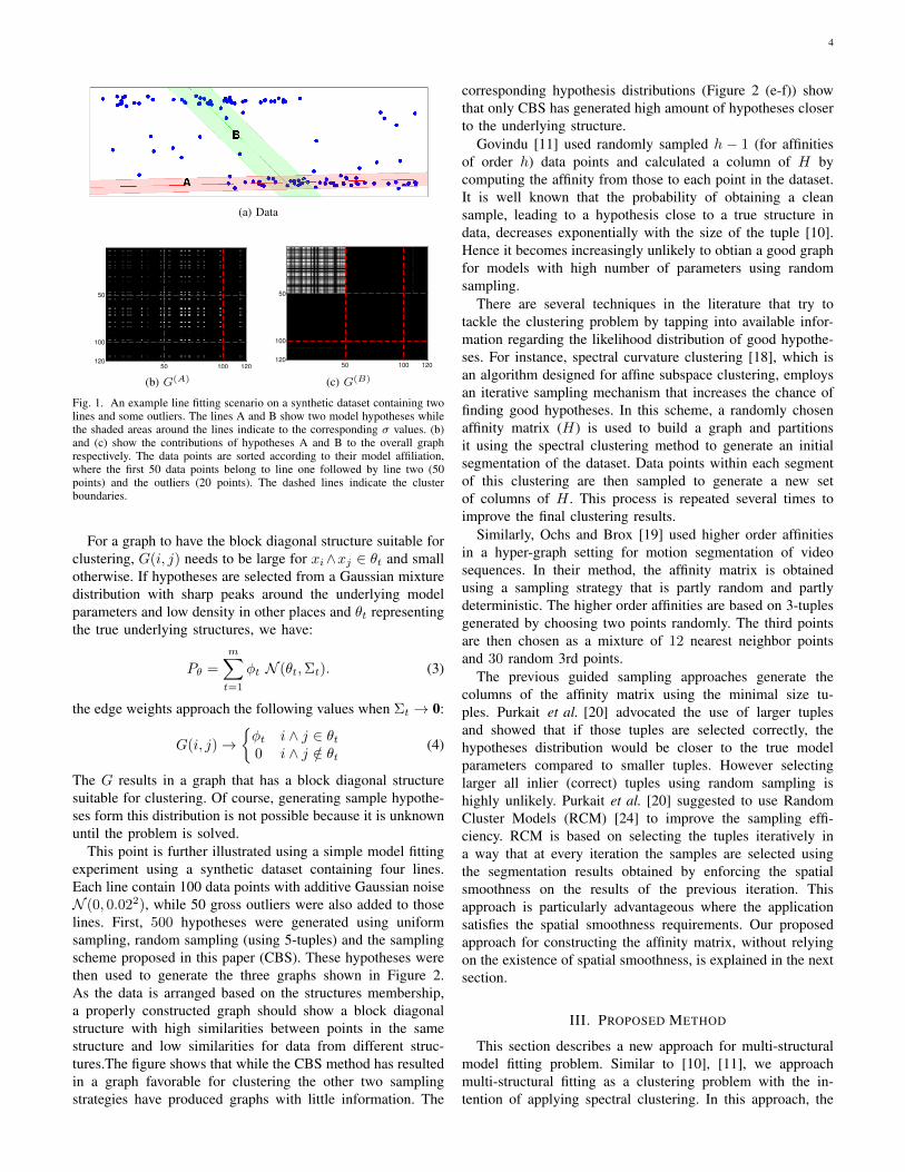
When a model hypothesis θl is close to an underlyingstructure in data (Hypothesis A in Figure 1a), the inlierpoints of that structure would have relatively small residualsand the resulting G(l) (Figure 1b) would have high affinitiesbetween the inliers and low affinity values for all other pointpairs (outlier-outlier, outlier-inlier). On the other hand, whena model hypothesis θl is far (in parameter space) from anyunderlying structure, the presumption is that the resultingresidual would be large, leading to a G(l) ≈ 0[N×N ]. However,as seen in Figure 1a (for Hypothesis B), this is not alwaysthe case in model fitting. It is highly likely that there existssome data points that give small residuals even for suchhypothesis (far from any underlying model) leading to highH(i, l) values. The resulting G(l) (Figure 1c) would have highaffinities between some unrelated points that can be seen asnoise in the overall graph. The effect of these bad hypothesiscan be amplified by the fact that the normalization factor,σ is often overestimated (using robust statistical methods)when the hypothesis θl is far (in parameter space) from anyunderlying structure. It is important to note that if none ofthe hypotheses (used in constructing the graph) are close toa underlying structure, then the overall graph would not havehigher affinities between the data points in that structure andthe clustering methods would not be able to segment thatstructure.

The above example shows that the sampling process influ-ences the level of noise in the graph. While spectral clusteringcan tolerate some level of noise, it has been proved that thisnoise level is related to the size of the smallest cluster we wantto recover (tolerable noise level goes up rapidly with the sizeof the smallest cluster) [23]. As model fitting often involvesrecovering small structures, it is highly important to limit thenoise level in the affinity matrix.

For any two data points xi, xj we can write:

G(i, j) =1

nH

nH∑l=1

e−(r2θl (i)+r

2θl

(j))2σ2︸ ︷︷ ︸

gij(θl)

as−−−→nH↑

∫Pθ · gij(θl) dθ

(2)For any model fitting problem with p > 2 there exists infinitenumber of models θl where gij(θl) → 1. This implies thatfor any two points, G(i, j) (according to Equation 2) can bemaximized or minimized by choosing Pθ accordingly.

4

(a) Data

50 100 120

50

100

120

(b) G(A)

50 100 120

50

100

120

(c) G(B)

Fig. 1. An example line fitting scenario on a synthetic dataset containing twolines and some outliers. The lines A and B show two model hypotheses whilethe shaded areas around the lines indicate to the corresponding σ values. (b)and (c) show the contributions of hypotheses A and B to the overall graphrespectively. The data points are sorted according to their model affiliation,where the first 50 data points belong to line one followed by line two (50points) and the outliers (20 points). The dashed lines indicate the clusterboundaries.

For a graph to have the block diagonal structure suitable forclustering, G(i, j) needs to be large for xi∧xj ∈ θt and smallotherwise. If hypotheses are selected from a Gaussian mixturedistribution with sharp peaks around the underlying modelparameters and low density in other places and θt representingthe true underlying structures, we have:

Pθ =

m∑t=1

φt N (θt,Σt). (3)

the edge weights approach the following values when Σt → 0:

G(i, j)→{φt i ∧ j ∈ θt0 i ∧ j /∈ θt

(4)

The G results in a graph that has a block diagonal structuresuitable for clustering. Of course, generating sample hypothe-ses form this distribution is not possible because it is unknownuntil the problem is solved.

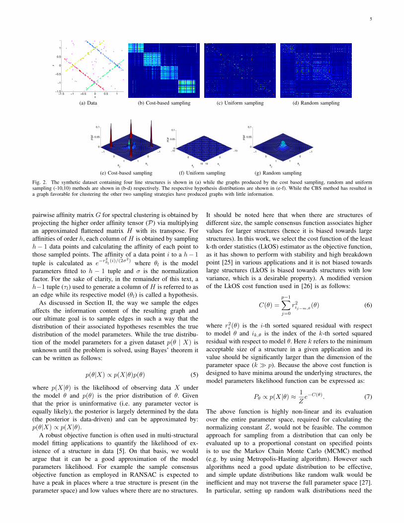
This point is further illustrated using a simple model fittingexperiment using a synthetic dataset containing four lines.Each line contain 100 data points with additive Gaussian noiseN (0, 0.022), while 50 gross outliers were also added to thoselines. First, 500 hypotheses were generated using uniformsampling, random sampling (using 5-tuples) and the samplingscheme proposed in this paper (CBS). These hypotheses werethen used to generate the three graphs shown in Figure 2.As the data is arranged based on the structures membership,a properly constructed graph should show a block diagonalstructure with high similarities between points in the samestructure and low similarities for data from different struc-tures.The figure shows that while the CBS method has resultedin a graph favorable for clustering the other two samplingstrategies have produced graphs with little information. The

corresponding hypothesis distributions (Figure 2 (e-f)) showthat only CBS has generated high amount of hypotheses closerto the underlying structure.

Govindu [11] used randomly sampled h − 1 (for affinitiesof order h) data points and calculated a column of H bycomputing the affinity from those to each point in the dataset.It is well known that the probability of obtaining a cleansample, leading to a hypothesis close to a true structure indata, decreases exponentially with the size of the tuple [10].Hence it becomes increasingly unlikely to obtian a good graphfor models with high number of parameters using randomsampling.

There are several techniques in the literature that try totackle the clustering problem by tapping into available infor-mation regarding the likelihood distribution of good hypothe-ses. For instance, spectral curvature clustering [18], which isan algorithm designed for affine subspace clustering, employsan iterative sampling mechanism that increases the chance offinding good hypotheses. In this scheme, a randomly chosenaffinity matrix (H) is used to build a graph and partitionsit using the spectral clustering method to generate an initialsegmentation of the dataset. Data points within each segmentof this clustering are then sampled to generate a new setof columns of H . This process is repeated several times toimprove the final clustering results.

Similarly, Ochs and Brox [19] used higher order affinitiesin a hyper-graph setting for motion segmentation of videosequences. In their method, the affinity matrix is obtainedusing a sampling strategy that is partly random and partlydeterministic. The higher order affinities are based on 3-tuplesgenerated by choosing two points randomly. The third pointsare then chosen as a mixture of 12 nearest neighbor pointsand 30 random 3rd points.

The previous guided sampling approaches generate thecolumns of the affinity matrix using the minimal size tu-ples. Purkait et al. [20] advocated the use of larger tuplesand showed that if those tuples are selected correctly, thehypotheses distribution would be closer to the true modelparameters compared to smaller tuples. However selectinglarger all inlier (correct) tuples using random sampling ishighly unlikely. Purkait et al. [20] suggested to use RandomCluster Models (RCM) [24] to improve the sampling effi-ciency. RCM is based on selecting the tuples iteratively ina way that at every iteration the samples are selected usingthe segmentation results obtained by enforcing the spatialsmoothness on the results of the previous iteration. Thisapproach is particularly advantageous where the applicationsatisfies the spatial smoothness requirements. Our proposedapproach for constructing the affinity matrix, without relyingon the existence of spatial smoothness, is explained in the nextsection.

III. PROPOSED METHOD

This section describes a new approach for multi-structuralmodel fitting problem. Similar to [10], [11], we approachmulti-structural fitting as a clustering problem with the in-tention of applying spectral clustering. In this approach, the

5

−1.5 −1 −0.5 0 0.5 1−1.5

−1

−0.5

0

0.5

1

5

x

y

(a) Data (b) Cost-based sampling (c) Uniform sampling (d) Random sampling

−1

0

1

−1

0

1

0

0.05

0.1

θ1θ

2

PD

F

(e) Cost-based sampling

−10

0

10

−10

0

10

0

0.05

0.1

θ1θ

2P

DF

(f) Uniform sampling

−1

0

1

−1

0

1

0

0.05

0.1

θ1θ

2

PD

F

(g) Random sampling

Fig. 2. The synthetic dataset containing four line structures is shown in (a) while the graphs produced by the cost based sampling, random and uniformsampling (-10,10) methods are shown in (b-d) respectively. The respective hypothesis distributions are shown in (e-f). While the CBS method has resulted ina graph favorable for clustering the other two sampling strategies have produced graphs with little information.

pairwise affinity matrix G for spectral clustering is obtained byprojecting the higher order affinity tensor (P) via multiplyingan approximated flattened matrix H with its transpose. Foraffinities of order h, each column of H is obtained by samplingh− 1 data points and calculating the affinity of each point tothose sampled points. The affinity of a data point i to a h− 1

tuple is calculated as e−r2θl

(i)/(2σ2) where θl is the modelparameters fitted to h − 1 tuple and σ is the normalizationfactor. For the sake of clarity, in the remainder of this text, ah−1 tuple (τl) used to generate a column of H is referred to asan edge while its respective model (θl) is called a hypothesis.

As discussed in Section II, the way we sample the edgesaffects the information content of the resulting graph andour ultimate goal is to sample edges in such a way that thedistribution of their associated hypotheses resembles the truedistribution of the model parameters. While the true distribu-tion of the model parameters for a given dataset p(θ | X) isunknown until the problem is solved, using Bayes’ theorem itcan be written as follows:

p(θ|X) ∝ p(X|θ)p(θ) (5)

where p(X|θ) is the likelihood of observing data X underthe model θ and p(θ) is the prior distribution of θ. Giventhat the prior is uninformative (i.e. any parameter vector isequally likely), the posterior is largely determined by the data(the posterior is data-driven) and can be approximated by:p(θ|X) ∝ p(X|θ).

A robust objective function is often used in multi-structuralmodel fitting applications to quantify the likelihood of ex-istence of a structure in data [5]. On that basis, we wouldargue that it can be a good approximation of the modelparameters likelihood. For example the sample consensusobjective function as employed in RANSAC is expected tohave a peak in places where a true structure is present (in theparameter space) and low values where there are no structures.

It should be noted here that when there are structures ofdifferent size, the sample consensus function associates highervalues for larger structures (hence it is biased towards largestructures). In this work, we select the cost function of the leastk-th order statistics (LkOS) estimator as the objective function,as it has shown to perform with stability and high breakdownpoint [25] in various applications and it is not biased towardslarge structures (LkOS is biased towards structures with lowvariance, which is a desirable property). A modified versionof the LkOS cost function used in [26] is as follows:

C(θ) =

p−1∑j=0

r2ij−m,θ

(θ) (6)

where r2i (θ) is the i-th sorted squared residual with respect

to model θ and ik,θ is the index of the k-th sorted squaredresidual with respect to model θ. Here k refers to the minimumacceptable size of a structure in a given application and itsvalue should be significantly larger than the dimension of theparameter space (k � p). Because the above cost function isdesigned to have minima around the underlying structures, themodel parameters likelihood function can be expressed as:

Pθ ∝ p(X|θ) ≈1

Ze−C(θ). (7)

The above function is highly non-linear and its evaluationover the entire parameter space, required for calculating thenormalizing constant Z, would not be feasible. The commonapproach for sampling from a distribution that can only beevaluated up to a proportional constant on specified pointsis to use the Markov Chain Monte Carlo (MCMC) method(e.g. by using Metropolis-Hasting algorithm). However suchalgorithms need a good update distribution to be effective,and simple update distributions like random walk would beinefficient and may not traverse the full parameter space [27].In particular, setting up random walk distributions need the

6

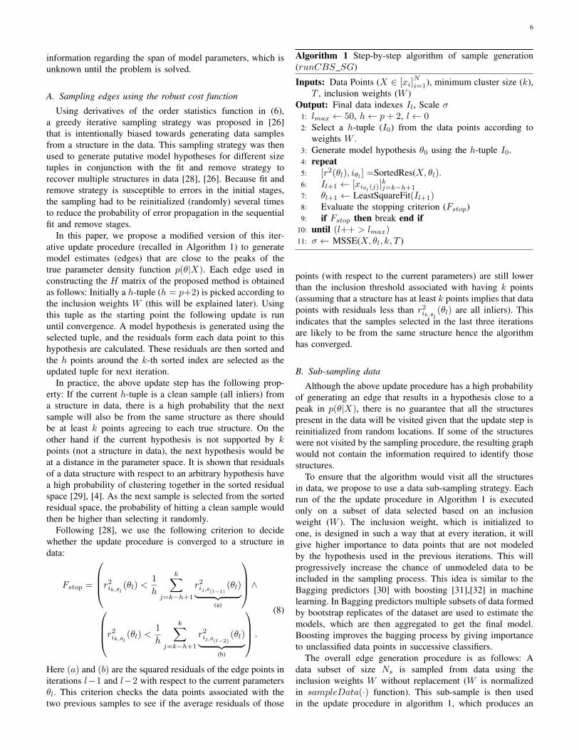
information regarding the span of model parameters, which isunknown until the problem is solved.

A. Sampling edges using the robust cost function

Using derivatives of the order statistics function in (6),a greedy iterative sampling strategy was proposed in [26]that is intentionally biased towards generating data samplesfrom a structure in the data. This sampling strategy was thenused to generate putative model hypotheses for different sizetuples in conjunction with the fit and remove strategy torecover multiple structures in data [28], [26]. Because fit andremove strategy is susceptible to errors in the initial stages,the sampling had to be reinitialized (randomly) several timesto reduce the probability of error propagation in the sequentialfit and remove stages.

In this paper, we propose a modified version of this iter-ative update procedure (recalled in Algorithm 1) to generatemodel estimates (edges) that are close to the peaks of thetrue parameter density function p(θ|X). Each edge used inconstructing the H matrix of the proposed method is obtainedas follows: Initially a h-tuple (h = p+2) is picked according tothe inclusion weights W (this will be explained later). Usingthis tuple as the starting point the following update is rununtil convergence. A model hypothesis is generated using theselected tuple, and the residuals form each data point to thishypothesis are calculated. These residuals are then sorted andthe h points around the k-th sorted index are selected as theupdated tuple for next iteration.

In practice, the above update step has the following prop-erty: If the current h-tuple is a clean sample (all inliers) froma structure in data, there is a high probability that the nextsample will also be from the same structure as there shouldbe at least k points agreeing to each true structure. On theother hand if the current hypothesis is not supported by kpoints (not a structure in data), the next hypothesis would beat a distance in the parameter space. It is shown that residualsof a data structure with respect to an arbitrary hypothesis havea high probability of clustering together in the sorted residualspace [29], [4]. As the next sample is selected from the sortedresidual space, the probability of hitting a clean sample wouldthen be higher than selecting it randomly.

Following [28], we use the following criterion to decidewhether the update procedure is converged to a structure indata:

Fstop =

r2ik,θl

(θl) <1

h

k∑j=k−h+1

r2ij,θ(l−1)

(θl)︸ ︷︷ ︸(a)

∧r2

ik,θl(θl) <

1

h

k∑j=k−h+1

r2ij,θ(l−2)

(θl)︸ ︷︷ ︸(b)

.

(8)

Here (a) and (b) are the squared residuals of the edge points initerations l−1 and l−2 with respect to the current parametersθl. This criterion checks the data points associated with thetwo previous samples to see if the average residuals of those

Algorithm 1 Step-by-step algorithm of sample generation(runCBS SG)

Inputs: Data Points (X ∈ [xi]Ni=1), minimum cluster size (k),

T , inclusion weights (W )Output: Final data indexes Il, Scale σ

1: lmax ← 50, h← p+ 2, l← 02: Select a h-tuple (I0) from the data points according to

weights W .3: Generate model hypothesis θ0 using the h-tuple I0.4: repeat5: [r2(θl), iθl ] =SortedRes(X, θl).6: Il+1 ← [xiθl (j)]

kj=k−h+1

7: θl+1 ← LeastSquareFit(Il+1)8: Evaluate the stopping criterion (Fstop)9: if Fstop then break end if

10: until (l++ > lmax)11: σ ← MSSE(X, θl, k, T )

points (with respect to the current parameters) are still lowerthan the inclusion threshold associated with having k points(assuming that a structure has at least k points implies that datapoints with residuals less than r2

ik,θl(θl) are all inliers). This

indicates that the samples selected in the last three iterationsare likely to be from the same structure hence the algorithmhas converged.

B. Sub-sampling data

Although the above update procedure has a high probabilityof generating an edge that results in a hypothesis close to apeak in p(θ|X), there is no guarantee that all the structurespresent in the data will be visited given that the update step isreinitialized from random locations. If some of the structureswere not visited by the sampling procedure, the resulting graphwould not contain the information required to identify thosestructures.

To ensure that the algorithm would visit all the structuresin data, we propose to use a data sub-sampling strategy. Eachrun of the the update procedure in Algorithm 1 is executedonly on a subset of data selected based on an inclusionweight (W ). The inclusion weight, which is initialized toone, is designed in such a way that at every iteration, it willgive higher importance to data points that are not modeledby the hypothesis used in the previous iterations. This willprogressively increase the chance of unmodeled data to beincluded in the sampling process. This idea is similar to theBagging predictors [30] with boosting [31],[32] in machinelearning. In Bagging predictors multiple subsets of data formedby bootstrap replicates of the dataset are used to estimate themodels, which are then aggregated to get the final model.Boosting improves the bagging process by giving importanceto unclassified data points in successive classifiers.

The overall edge generation procedure is as follows: Adata subset of size Ns is sampled from data using theinclusion weights W without replacement (W is normalizedin sampleData(·) function). This sub-sample is then usedin the update procedure in algorithm 1, which produces an

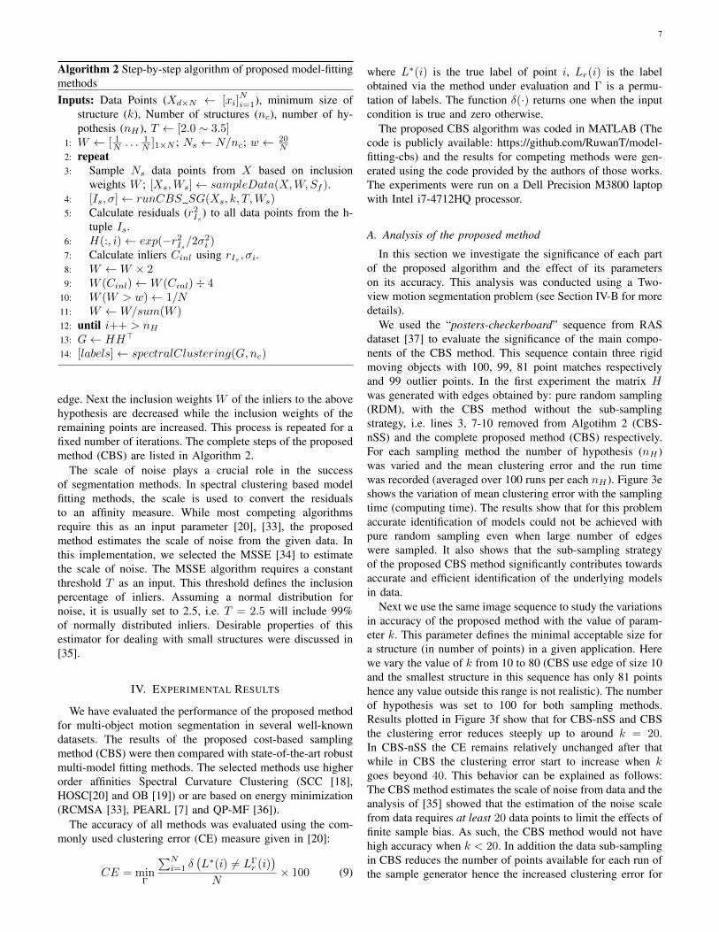
7

Algorithm 2 Step-by-step algorithm of proposed model-fittingmethodsInputs: Data Points (Xd×N ← [xi]

Ni=1), minimum size of

structure (k), Number of structures (nc), number of hy-pothesis (nH ), T ← [2.0 ∼ 3.5]

1: W ← [ 1N . . . 1

N ]1×N ; Ns ← N/nc; w ← 20N

2: repeat3: Sample Ns data points from X based on inclusion

weights W ; [Xs,Ws]← sampleData(X,W,Sf ).4: [Is, σ]← runCBS SG(Xs, k, T,Ws)5: Calculate residuals (r2

Is) to all data points from the h-

tuple Is.6: H(:, i)← exp(−r2

Is/2σ2

i )7: Calculate inliers Cinl using rIs , σi.8: W ←W × 29: W (Cinl)←W (Cinl)÷ 4

10: W (W > w)← 1/N11: W ←W/sum(W )12: until i++ > nH13: G← HH>

14: [labels]← spectralClustering(G,nc)

edge. Next the inclusion weights W of the inliers to the abovehypothesis are decreased while the inclusion weights of theremaining points are increased. This process is repeated for afixed number of iterations. The complete steps of the proposedmethod (CBS) are listed in Algorithm 2.

The scale of noise plays a crucial role in the successof segmentation methods. In spectral clustering based modelfitting methods, the scale is used to convert the residualsto an affinity measure. While most competing algorithmsrequire this as an input parameter [20], [33], the proposedmethod estimates the scale of noise from the given data. Inthis implementation, we selected the MSSE [34] to estimatethe scale of noise. The MSSE algorithm requires a constantthreshold T as an input. This threshold defines the inclusionpercentage of inliers. Assuming a normal distribution fornoise, it is usually set to 2.5, i.e. T = 2.5 will include 99%of normally distributed inliers. Desirable properties of thisestimator for dealing with small structures were discussed in[35].

IV. EXPERIMENTAL RESULTS

We have evaluated the performance of the proposed methodfor multi-object motion segmentation in several well-knowndatasets. The results of the proposed cost-based samplingmethod (CBS) were then compared with state-of-the-art robustmulti-model fitting methods. The selected methods use higherorder affinities Spectral Curvature Clustering (SCC [18],HOSC[20] and OB [19]) or are based on energy minimization(RCMSA [33], PEARL [7] and QP-MF [36]).

The accuracy of all methods was evaluated using the com-monly used clustering error (CE) measure given in [20]:

CE = minΓ

∑Ni=1 δ

(L∗(i) 6= LΓ

r (i))

N× 100 (9)

where L∗(i) is the true label of point i, Lr(i) is the labelobtained via the method under evaluation and Γ is a permu-tation of labels. The function δ(·) returns one when the inputcondition is true and zero otherwise.

The proposed CBS algorithm was coded in MATLAB (Thecode is publicly available: https://github.com/RuwanT/model-fitting-cbs) and the results for competing methods were gen-erated using the code provided by the authors of those works.The experiments were run on a Dell Precision M3800 laptopwith Intel i7-4712HQ processor.

A. Analysis of the proposed method

In this section we investigate the significance of each partof the proposed algorithm and the effect of its parameterson its accuracy. This analysis was conducted using a Two-view motion segmentation problem (see Section IV-B for moredetails).

We used the “posters-checkerboard” sequence from RASdataset [37] to evaluate the significance of the main compo-nents of the CBS method. This sequence contain three rigidmoving objects with 100, 99, 81 point matches respectivelyand 99 outlier points. In the first experiment the matrix Hwas generated with edges obtained by: pure random sampling(RDM), with the CBS method without the sub-samplingstrategy, i.e. lines 3, 7-10 removed from Algotihm 2 (CBS-nSS) and the complete proposed method (CBS) respectively.For each sampling method the number of hypothesis (nH )was varied and the mean clustering error and the run timewas recorded (averaged over 100 runs per each nH ). Figure 3eshows the variation of mean clustering error with the samplingtime (computing time). The results show that for this problemaccurate identification of models could not be achieved withpure random sampling even when large number of edgeswere sampled. It also shows that the sub-sampling strategyof the proposed CBS method significantly contributes towardsaccurate and efficient identification of the underlying modelsin data.

Next we use the same image sequence to study the variationsin accuracy of the proposed method with the value of param-eter k. This parameter defines the minimal acceptable size fora structure (in number of points) in a given application. Herewe vary the value of k from 10 to 80 (CBS use edge of size 10and the smallest structure in this sequence has only 81 pointshence any value outside this range is not realistic). The numberof hypothesis was set to 100 for both sampling methods.Results plotted in Figure 3f show that for CBS-nSS and CBSthe clustering error reduces steeply up to around k = 20.In CBS-nSS the CE remains relatively unchanged after thatwhile in CBS the clustering error start to increase when kgoes beyond 40. This behavior can be explained as follows:The CBS method estimates the scale of noise from data and theanalysis of [35] showed that the estimation of the noise scalefrom data requires at least 20 data points to limit the effects offinite sample bias. As such, the CBS method would not havehigh accuracy when k < 20. In addition the data sub-samplingin CBS reduces the number of points available for each run ofthe sample generator hence the increased clustering error for

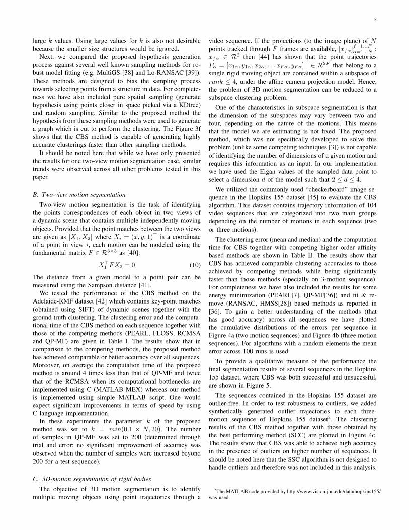
8

large k values. Using large values for k is also not desirablebecause the smaller size structures would be ignored.

Next, we compared the proposed hypothesis generationprocess against several well known sampling methods for ro-bust model fitting (e.g. MultiGS [38] and Lo-RANSAC [39]).These methods are designed to bias the sampling processtowards selecting points from a structure in data. For complete-ness we have also included pure spatial sampling (generatehypothesis using points closer in space picked via a KDtree)and random sampling. Similar to the proposed method thehypothesis from these sampling methods were used to generatea graph which is cut to perform the clustering. The Figure 3fshows that the CBS method is capable of generating highlyaccurate clusterings faster than other sampling methods.

It should be noted here that while we have only presentedthe results for one two-view motion segmentation case, similartrends were observed across all other problems tested in thispaper.

B. Two-view motion segmentation

Two-view motion segmentation is the task of identifyingthe points correspondences of each object in two views ofa dynamic scene that contains multiple independently movingobjects. Provided that the point matches between the two viewsare given as [X1, X2] where Xi = (x, y, 1)> is a coordinateof a point in view i, each motion can be modeled using thefundamental matrix F ∈ R3×3 as [40]:

X>1 FX2 = 0 (10)

The distance from a given model to a point pair can bemeasured using the Sampson distance [41].

We tested the performance of the CBS method on theAdelaide-RMF dataset [42] which contains key-point matches(obtained using SIFT) of dynamic scenes together with theground truth clustering. The clustering error and the computa-tional time of the CBS method on each sequence together withthose of the competing methods (PEARL, FLOSS, RCMSAand QP-MF) are given in Table I. The results show that incomparison to the competing methods, the proposed methodhas achieved comparable or better accuracy over all sequences.Moreover, on average the computation time of the proposedmethod is around 4 times less than that of QP-MF and twicethat of the RCMSA when its computational bottlenecks areimplemented using C (MATLAB MEX) whereas our methodis implemented using simple MATLAB script. One wouldexpect significant improvements in terms of speed by usingC language implementation.

In these experiments the parameter k of the proposedmethod was set to k = min(0.1 × N, 20). The numberof samples in QP-MF was set to 200 (determined throughtrial and error: no significant improvement of accuracy wasobserved when the number of samples were increased beyond200 for a test sequence).

C. 3D-motion segmentation of rigid bodies

The objective of 3D motion segmentation is to identifymultiple moving objects using point trajectories through a

video sequence. If the projections (to the image plane) of Npoints tracked through F frames are available, [xfα]

f=1...Fα=1...N :

xfα ∈ R2 then [44] has shown that the point trajectoriesPα = [x1α, y1α, x2α, . . . xFα, yFα]

> ∈ R2F that belong to asingle rigid moving object are contained within a subspace ofrank ≤ 4, under the affine camera projection model. Hence,the problem of 3D motion segmentation can be reduced to asubspace clustering problem.

One of the characteristics in subspace segmentation is thatthe dimension of the subspaces may vary between two andfour, depending on the nature of the motions. This meansthat the model we are estimating is not fixed. The proposedmethod, which was not specifically developed to solve thisproblem (unlike some competing techniques [3]) is not capableof identifying the number of dimensions of a given motion andrequires this information as an input. In our implementationwe have used the Eigan values of the sampled data point toselect a dimension d of the model such that 2 ≤ d ≤ 4.

We utilized the commonly used “checkerboard” image se-quence in the Hopkins 155 dataset [45] to evaluate the CBSalgorithm. This dataset contains trajectory information of 104video sequences that are categorized into two main groupsdepending on the number of motions in each sequence (twoor three motions).

The clustering error (mean and median) and the computationtime for CBS together with competing higher order affinitybased methods are shown in Table II. The results show thatCBS has achieved comparable clustering accuracies to thoseachieved by competing methods while being significantlyfaster than those methods (specially on 3-motion sequence).For completeness we have also included the results for someenergy minimization (PEARL[7], QP-MF[36]) and fit & re-move (RANSAC, HMSS[28]) based methods as reported in[36]. To gain a better understanding of the methods (thathas good accuracy) across all sequences we have plottedthe cumulative distributions of the errors per sequence inFigure 4a (two motion sequences) and Figure 4b (three motionsequences). For algorithms with a random elements the meanerror across 100 runs is used.

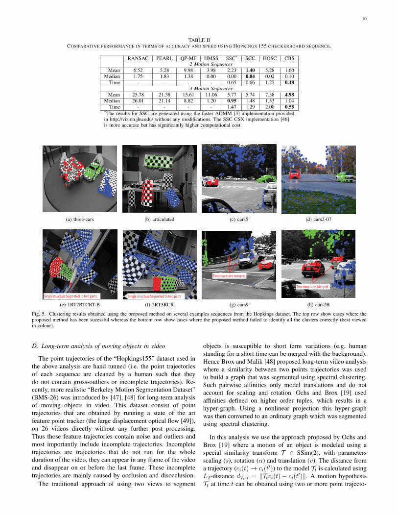
To provide a qualitative measure of the performance thefinal segmentation results of several sequences in the Hopkins155 dataset, where CBS was both successful and unsucessful,are shown in Figure 5.

The sequences contained in the Hopkins 155 dataset areoutlier-free. In order to test robustness to outliers, we addedsynthetically generated outlier trajectories to each three-motion sequence of Hopkins 155 dataset2. The clusteringresults of the CBS method together with those obtained bythe best performing method (SCC) are plotted in Figure 4c.The results show that CBS was able to achieve high accuracyin the presence of outliers on higher number of sequences. Itshould be noted here that the SSC algorithm is not designed tohandle outliers and therefore was not included in this analysis.

2The MATLAB code provided by http://www.vision.jhu.edu/data/hopkins155/was used.

9

OutliersGroup 1Group 2Group 3

(a) Ground truth

OutliersGroup 1Group 2Group 3

(b) Random

OutliersGroup 1Group 2Group 3

(c) CBS-nSS

OutliersGroup 1Group 2Group 3

(d) CBS

0 0.5 1 1.5 2 2.50

10

20

30

40

50

60

70

80

Sampling Time (s)

Clu

ste

rin

g

Err

or(

%)

RDMCBS−nSSCBS

1000 edges

50 edges

50 edges

(e)

0 20 40 60 800

5

10

15

20

25

30

35

40

Value of parameter k

Clu

stering E

rror

(%)

CBSCBS−nSS

(f)

0 0.5 1 1.5 2 2.50

10

20

30

40

50

60

70

80

Sampling Time (s)

Clu

ste

rin

g

Err

or(

%)

RDMSpatialMultiGSLo−RANSACCBS

200 edges50 edges

(g)

Fig. 3. The results on “posters-checkerboard” sequence, 3a shows the ground truth clustering while 3b - 3d shows the clustering obtained with RDM, CBS-nssand CBS at 1s. 3e and 3f shows the variation of clustering error with time and the value of parameter k respectively, while 3g shows the variation in clusteringerror with the value of parameter k (best viewed in color).

TABLE ITWO-VIEW MOTION SEGMENTATION RESULTS ON ADELAIDE-RMF DATASET. THE MEDIAN CE VALUES OF PEARL AND FLOSS [43] REPOTED IN [33]

ARE USED HERE.

PEARL FLOSS QP-MF RCMSA CBSMedian CE Median CE Median CE Time Median CE Time Median CE Time

biscuitbookbox 8.11 11.58 5.02 4.78 7.72 0.56 0.00 0.95boardgame 16.85 17.92 17.38 4.49 12.09 0.50 11.28 0.99

breadcartoychips 12.24 15.82 8.65 4.52 9.97 0.64 5.63 0.93breadcubechips 9.57 11.74 3.04 4.47 9.78 0.54 0.87 0.85

breadtoycar 10.24 11.75 6.33 4.20 8.73 0.44 3.96 0.75carchipscube 10.30 16.97 17.27 3.59 4.85 0.42 2.44 0.65

cubebreadtoychips 9.02 11.31 2.14 5.07 8.87 0.71 1.91 1.13dinobooks 19.17 20.28 17.92 5.20 17.50 0.73 12.98 1.25

toycubecar 12.00 13.75 14.50 3.71 11.00 0.38 19.19 0.70

0 10 20 30 40 500

20

40

60

80

100

Clustering Error (%)

Perc

enta

ge o

f S

equence

s

CBSSCCHOSCSSC

(a) Two motion sequences

0 10 20 30 40 500

20

40

60

80

100

Clustering Error (%)

Perc

enta

ge o

f S

equence

s

CBSSCCHOSCSSC

(b) Three motion sequences

0 10 20 30 40 500

20

40

60

80

100

Clustering Error (%)

Perc

enta

ge o

f S

equence

s

CBSSCC

(c) Three motion with Outliers

Fig. 4. Cumulative distributions of the clustering errors (CE) per sequence of the Hopkings dataset. Figure 4a Two motion sequences, Figure 4b Three motionsequences and Figure 4c Three motion sequences with added synthetic outliers.

10

TABLE IICOMPARATIVE PERFORMANCE IN TERMS OF ACCURACY AND SPEED USING HOPKINGS 155 CHECKERBOARD SEQUENCE.

RANSAC PEARL QP-MF HMSS SSC* SCC HOSC CBS2 Motion Sequences

Mean 6.52 5.28 9.98 3.98 2.23 1.40 5.28 1.60Median 1.75 1.83 1.38 0.00 0.00 0.04 0.02 0.10

Time - - - - 0.65 0.66 1.27 0.483 Motion Sequences

Mean 25.78 21.38 15.61 11.06 5.77 5.74 7.38 4.98Median 26.01 21.14 8.82 1.20 0.95 1.48 1.53 1.04

Time - - - - 1.47 1.29 2.00 0.55*The results for SSC are generated using the faster ADMM [3] implementation providedin http://vision.jhu.edu/ without any modifications. The SSC CSX implementation [46]is more accurate but has significantly higher computational cost.

(a) three-cars

(b) articulated (c) cars5

(d) cars2-07

Single structure Segmeted to two parts

(e) 1RT2RTCRT-B

Single structure Segmeted to two parts

(f) 2RT3RCR

Two structures merged

(g) cars9

Two structures Merged

(h) cars2B

Fig. 5. Clustering results obtained using the proposed method on several examples sequences from the Hopkings dataset. The top row show cases where theproposed method has been sucessful whereas the bottom row show cases where the proposed method failed to identify all the clusters correctly (best viewedin colour).

D. Long-term analysis of moving objects in video

The point trajectories of the “Hopkings155” dataset used inthe above analysis are hand tunned (i.e. the point trajectoriesof each sequence are cleaned by a human such that theydo not contain gross-outliers or incomplete trajectories). Re-cently, more realistic “Berkeley Motion Segmentation Dataset”(BMS-26) was introduced by [47], [48] for long-term analysisof moving objects in video. This dataset consist of pointtrajectories that are obtained by running a state of the artfeature point tracker (the large displacement optical flow [49]),on 26 videos directly without any further post processing.Thus those feature trajectories contain noise and outliers andmost importantly include incomplete trajectories. Incompletetrajectories are trajectories that do not run for the wholeduration of the video, they can appear in any frame of the videoand disappear on or before the last frame. These incompletetrajectories are mainly caused by occlusion and disocclusion.

The traditional approach of using two views to segment

objects is susceptible to short term variations (e.g. humanstanding for a short time can be merged with the background).Hence Brox and Malik [48] proposed long-term video analysiswhere a similarity between two points trajectories was usedto build a graph that was segmented using spectral clustering.Such pairwise affinities only model translations and do notaccount for scaling and rotation. Ochs and Brox [19] usedaffinities defined on higher order tuples, which results in ahyper-graph. Using a nonlinear projection this hyper-graphwas then converted to an ordinary graph which was segmentedusing spectral clustering.

In this analysis we use the approach proposed by Ochs andBrox [19] where a motion of an object is modeled using aspecial similarity transform T ∈ SSim(2), with parametersscaling (s), rotation (α) and translation (v). The distance froma trajectory (ci(t)→ ci(t

′)) to the model Tt is calculated usingL2-distance dTt,i = ‖Ttci(t)− ci(t′)‖. A motion hypothesisTt at time t can be obtained using two or more point trajecto-

11

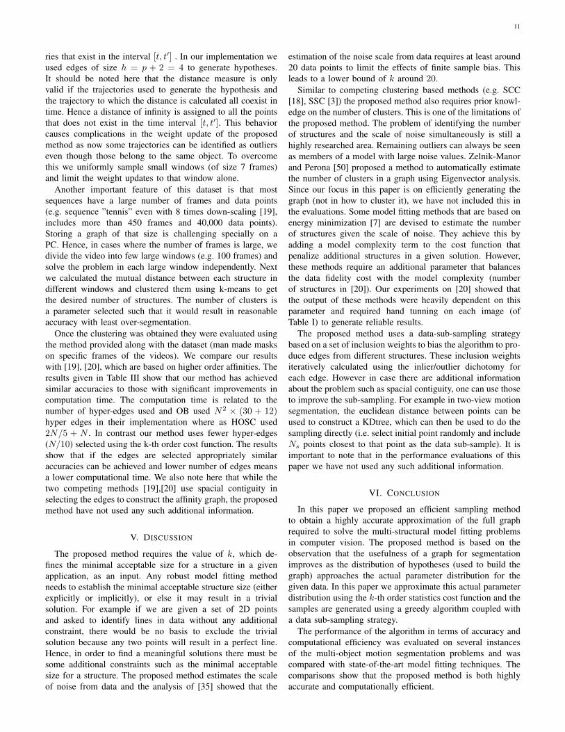
ries that exist in the interval [t, t′] . In our implementation weused edges of size h = p + 2 = 4 to generate hypotheses.It should be noted here that the distance measure is onlyvalid if the trajectories used to generate the hypothesis andthe trajectory to which the distance is calculated all coexist intime. Hence a distance of infinity is assigned to all the pointsthat does not exist in the time interval [t, t′]. This behaviorcauses complications in the weight update of the proposedmethod as now some trajectories can be identified as outlierseven though those belong to the same object. To overcomethis we uniformly sample small windows (of size 7 frames)and limit the weight updates to that window alone.

Another important feature of this dataset is that mostsequences have a large number of frames and data points(e.g. sequence ”tennis” even with 8 times down-scaling [19],includes more than 450 frames and 40,000 data points).Storing a graph of that size is challenging specially on aPC. Hence, in cases where the number of frames is large, wedivide the video into few large windows (e.g. 100 frames) andsolve the problem in each large window independently. Nextwe calculated the mutual distance between each structure indifferent windows and clustered them using k-means to getthe desired number of structures. The number of clusters isa parameter selected such that it would result in reasonableaccuracy with least over-segmentation.

Once the clustering was obtained they were evaluated usingthe method provided along with the dataset (man made maskson specific frames of the videos). We compare our resultswith [19], [20], which are based on higher order affinities. Theresults given in Table III show that our method has achievedsimilar accuracies to those with significant improvements incomputation time. The computation time is related to thenumber of hyper-edges used and OB used N2 × (30 + 12)hyper edges in their implementation where as HOSC used2N/5 + N . In contrast our method uses fewer hyper-edges(N/10) selected using the k-th order cost function. The resultsshow that if the edges are selected appropriately similaraccuracies can be achieved and lower number of edges meansa lower computational time. We also note here that while thetwo competing methods [19],[20] use spacial contiguity inselecting the edges to construct the affinity graph, the proposedmethod have not used any such additional information.

V. DISCUSSION

The proposed method requires the value of k, which de-fines the minimal acceptable size for a structure in a givenapplication, as an input. Any robust model fitting methodneeds to establish the minimal acceptable structure size (eitherexplicitly or implicitly), or else it may result in a trivialsolution. For example if we are given a set of 2D pointsand asked to identify lines in data without any additionalconstraint, there would be no basis to exclude the trivialsolution because any two points will result in a perfect line.Hence, in order to find a meaningful solutions there must besome additional constraints such as the minimal acceptablesize for a structure. The proposed method estimates the scaleof noise from data and the analysis of [35] showed that the

estimation of the noise scale from data requires at least around20 data points to limit the effects of finite sample bias. Thisleads to a lower bound of k around 20.

Similar to competing clustering based methods (e.g. SCC[18], SSC [3]) the proposed method also requires prior knowl-edge on the number of clusters. This is one of the limitations ofthe proposed method. The problem of identifying the numberof structures and the scale of noise simultaneously is still ahighly researched area. Remaining outliers can always be seenas members of a model with large noise values. Zelnik-Manorand Perona [50] proposed a method to automatically estimatethe number of clusters in a graph using Eigenvector analysis.Since our focus in this paper is on efficiently generating thegraph (not in how to cluster it), we have not included this inthe evaluations. Some model fitting methods that are based onenergy minimization [7] are devised to estimate the numberof structures given the scale of noise. They achieve this byadding a model complexity term to the cost function thatpenalize additional structures in a given solution. However,these methods require an additional parameter that balancesthe data fidelity cost with the model complexity (numberof structures in [20]). Our experiments on [20] showed thatthe output of these methods were heavily dependent on thisparameter and required hand tunning on each image (ofTable I) to generate reliable results.

The proposed method uses a data-sub-sampling strategybased on a set of inclusion weights to bias the algorithm to pro-duce edges from different structures. These inclusion weightsiteratively calculated using the inlier/outlier dichotomy foreach edge. However in case there are additional informationabout the problem such as spacial contiguity, one can use thoseto improve the sub-sampling. For example in two-view motionsegmentation, the euclidean distance between points can beused to construct a KDtree, which can then be used to do thesampling directly (i.e. select initial point randomly and includeNs points closest to that point as the data sub-sample). It isimportant to note that in the performance evaluations of thispaper we have not used any such additional information.

VI. CONCLUSION

In this paper we proposed an efficient sampling methodto obtain a highly accurate approximation of the full graphrequired to solve the multi-structural model fitting problemsin computer vision. The proposed method is based on theobservation that the usefulness of a graph for segmentationimproves as the distribution of hypotheses (used to build thegraph) approaches the actual parameter distribution for thegiven data. In this paper we approximate this actual parameterdistribution using the k-th order statistics cost function and thesamples are generated using a greedy algorithm coupled witha data sub-sampling strategy.

The performance of the algorithm in terms of accuracy andcomputational efficiency was evaluated on several instancesof the multi-object motion segmentation problems and wascompared with state-of-the-art model fitting techniques. Thecomparisons show that the proposed method is both highlyaccurate and computationally efficient.

12

TABLE IIIMOTION SEGMENTATION RESULTS ON BERKELEY MOTION SEGMENTATION DATASET (BMS-26).

Density Overall error Average error Over-segmentation rate Extracted objects Total Time(s)OB 1.03% 5.68% 24.74% 1.48 30 434545

HOSC 1.03% 8.05% 27.84% 2.1 22 11966CBS 1.03% 7.80% 22.60% 2.08 22 7875

ACKNOWLEDGMENT

This research was partly supported under Australian Re-search Council (ARC) Linkage Projects funding scheme.

REFERENCES

[1] M. A. Fischler and R. C. Bolles, “Random sample con-sensus: A paradigm for model fitting with applicationsto image analysis and automated cartography,” Commun.ACM, vol. 24, no. 6, pp. 381–395, Jun. 1981.

[2] A. Delong, L. Gorelick, O. Veksler, and Y. Boykov, “Min-imizing energies with hierarchical costs,” InternationalJournal of Computer Vision, vol. 100, no. 1, pp. 38–58,2012.

[3] E. Elhamifar and R. Vidal, “Sparse subspace clustering:Algorithm, theory, and applications,” Pattern Analysis andMachine Intelligence, IEEE Transactions on, vol. 35,no. 11, pp. 2765–2781, 2013.

[4] C. Haifeng and P. Meer, “Robust regression with pro-jection based m-estimators,” in Proceedings. Ninth IEEEInternational Conference on Computer Vision, 2003, pp.878–885 vol.2.

[5] C. V. Stewart, “Bias in robust estimation caused by discon-tinuities and multiple structures,” IEEE Transactions onPattern Analysis and Machine Intelligence, vol. 19, no. 8,pp. 818–833, 1997.

[6] M. Zuliani, C. S. Kenney, and B. S. Manjunath, “Themultiransac algorithm and its application to detect pla-nar homographies,” in IEEE International Conference onImage Processing, ICIP., vol. 3, 2005, pp. III–153–6.

[7] Y. Boykov, O. Veksler, and R. Zabih, “Fast approximateenergy minimization via graph cuts,” Pattern Analysisand Machine Intelligence, IEEE Transactions on, vol. 23,no. 11, pp. 1222–1239, 2001.

[8] E. J. Candes, X. Li, Y. Ma, and J. Wright, “Robust prin-cipal component analysis?” Journal of the ACM (JACM),vol. 58, no. 3, p. 11, 2011.

[9] R. Cabral, F. De La Torre, J. P. Costeira, andA. Bernardino, “Unifying nuclear norm and bilinear fac-torization approaches for low-rank matrix decomposition,”in Proceedings of the IEEE International Conference onComputer Vision, 2013, pp. 2488–2495.

[10] S. Agarwal, L. Jongwoo, L. Zelnik-Manor, P. Perona,D. Kriegman, and S. Belongie, “Beyond pairwise cluster-ing,” in IEEE Computer Society Conference on ComputerVision and Pattern Recognition, CVPR., vol. 2, 2005, pp.838–845.

[11] V. M. Govindu, “A tensor decomposition for geometricgrouping and segmentation,” in IEEE Computer SocietyConference on Computer Vision and Pattern Recognition,CVPR., vol. 1, 2005, pp. 1150–1157 vol. 1.

[12] G. Liu, Z. Lin, S. Yan, J. Sun, Y. Yu, and Y. Ma, “Robustrecovery of subspace structures by low-rank representa-tion,” IEEE Transactions on Pattern Analysis and MachineIntelligence, vol. 35, no. 1, pp. 171–184, 2013.

[13] G. Liu, H. Xu, J. Tang, Q. Liu, and S. Yan, “A deter-ministic analysis for lrr,” IEEE Transactions on PatternAnalysis and Machine Intelligence, vol. 38, no. 3, pp. 417–430, 2016.

[14] J. Wang, D. Shi, D. Cheng, Y. Zhang, and J. Gao, “Lrsr:Low-rank-sparse representation for subspace clustering,”Neurocomputing, 2016.

[15] E. Kim, M. Lee, and S. Oh, “Robust elastic-net subspacerepresentation,” IEEE Transactions on Image Processing,2016.

[16] B. Poling and G. Lerman, “A new approach to two-viewmotion segmentation using global dimension minimiza-tion,” International Journal of Computer Vision, vol. 108,no. 3, pp. 165–185, 2014.

[17] A. Y. Ng, M. I. Jordan, and Y. Weiss, “On spectralclustering: Analysis and an algorithm,” in Advances inNeural Information Processing Systems 14, T. Dietterich,S. Becker, and Z. Ghahramani, Eds. MIT Press, 2002,pp. 849–856.

[18] G. Chen and G. Lerman, “Spectral curvature clustering(scc),” International Journal of Computer Vision, vol. 81,no. 3, pp. 317–330, 2009.

[19] P. Ochs and T. Brox, “Higher order motion models andspectral clustering,” in IEEE Conference on ComputerVision and Pattern Recognition, CVPR., 2012, pp. 614–621.

[20] P. Purkait, T.-J. Chin, H. Ackermann, and D. Suter,Clustering with Hypergraphs: The Case for Large Hyper-edges, ser. Lecture Notes in Computer Science. SpringerInternational Publishing, 2014, vol. 8692, ch. 44, pp. 672–687.

[21] B. Li, Y. Zhang, Z. Lin, and H. Lu, “Subspace clusteringby mixture of gaussian regression,” in Proceedings ofthe IEEE Conference on Computer Vision and PatternRecognition, 2015, pp. 2094–2102.

[22] T. Zhang, A. Szlam, Y. Wang, and G. Lerman, “Hybridlinear modeling via local best-fit flats,” International jour-nal of computer vision, vol. 100, no. 3, pp. 217–240, 2012.

[23] S. Balakrishnan, M. Xu, A. Krishnamurthy, and A. Singh,“Noise thresholds for spectral clustering,” in Advancesin Neural Information Processing Systems 24, J. Shawe-Taylor, R. S. Zemel, P. L. Bartlett, F. Pereira, and K. Q.Weinberger, Eds. Curran Associates, Inc., 2011, pp. 954–962. [Online].

[24] R. H. Swendsen and J.-S. Wang, “Nonuniversal criticaldynamics in monte carlo simulations,” Physical review

13

letters, vol. 58, no. 2, p. 86, 1987.[25] P. J. Rousseeuw and A. M. Leroy, Robust regression and

outlier detection. John Wiley & Sons, 2005, vol. 589.[26] A. Bab-Hadiashar and R. Hoseinnezhad, “Bridging pa-

rameter and data spaces for fast robust estimation incomputer vision,” in Digital Image Computing: Tech-niques and Applications (DICTA), 2008, 2008, ConferenceProceedings, pp. 1–8.

[27] C. Andrieu, N. de Freitas, A. Doucet, and M. Jordan,“An introduction to mcmc for machine learning,” MachineLearning, vol. 50, no. 1-2, pp. 5–43, 2003.

[28] R. Tennakoon, A. Bab-Hadiashar, Z. Cao, R. Hosein-nezhad, and D. Suter, “Robust model fitting using higherthan minimal subset sampling,” Pattern Analysis and Ma-chine Intelligence, IEEE Transactions on, vol. PP, no. 99,pp. 1–1, 2015.

[29] R. Toldo and A. Fusiello, Robust Multiple StructuresEstimation with J-Linkage, ser. Lecture Notes in ComputerScience. Springer Berlin Heidelberg, 2008, vol. 5302,book section 41, pp. 537–547.

[30] L. Breiman, “Bagging predictors,” Machine Learning,vol. 24, no. 2, pp. 123–140, 1996.

[31] Y. Freund and R. E. Schapire, “Experiments with a newboosting algorithm,” in ICML Vol. 96, pp. 148-156, 1996,Conference Proceedings.

[32] ——, “A decision-theoretic generalization of on-linelearning and an application to boosting,” Journal of Com-puter and System Sciences, vol. 55, no. 1, pp. 119–139,1997.

[33] T. T. Pham, C. Tat-Jun, Y. Jin, and D. Suter, “Therandom cluster model for robust geometric fitting,” PatternAnalysis and Machine Intelligence, IEEE Transactions on,vol. 36, no. 8, pp. 1658–1671, 2014.

[34] A. Bab-Hadiashar and D. Suter, “Robust segmentationof visual data using ranked unbiased scale estimate,”Robotica, vol. 17, no. 06, pp. 649–660, 1999.

[35] R. Hoseinnezhad, A. Bab-Hadiashar, and D. Suter, “Fi-nite sample bias of robust estimators in segmentation ofclosely spaced structures: a comparative study,” Journalof mathematical Imaging and Vision, vol. 37, no. 1, pp.66–84, 2010.

[36] Y. Jin, C. Tat-Jun, and D. Suter, “A global optimiza-tion approach to robust multi-model fitting,” in IEEEConference on Computer Vision and Pattern Recognition(CVPR), 2011, Conference Proceedings, pp. 2041–2048.

[37] S. Rao, A. Yang, S. S. Sastry, and Y. Ma, “Robustalgebraic segmentation of mixed rigid-body and planarmotions from two views,” International Journal of Com-puter Vision, vol. 88, no. 3, pp. 425–446, 2010.

[38] C. Tat-Jun, Y. Jin, and D. Suter, “Accelerated hypothesisgeneration for multistructure data via preference analysis,”Pattern Analysis and Machine Intelligence, IEEE Trans-actions on, vol. 34, no. 4, pp. 625–638, 2012.

[39] O. Chum, J. Matas, and J. Kittler, “Locally optimizedransac,” in Lecture Notes in Computer Science (includingsubseries Lecture Notes in Artificial Intelligence and Lec-ture Notes in Bioinformatics), 2003, vol. 2781, pp. 236–243.

[40] P. H. S. Torr and D. W. Murray, “The developmentand comparison of robust methods for estimating thefundamental matrix,” International Journal of ComputerVision, vol. 24, no. 3, pp. 271–300, 1997.

[41] R. Hartley and A. Zisserman, Multiple view geometry incomputer vision. Cambridge university press, 2003.

[42] W. Hoi Sim, C. Tat-Jun, Y. Jin, and D. Suter, “Dynamicand hierarchical multi-structure geometric model fitting,”in Computer Vision (ICCV), 2011 IEEE InternationalConference on, 2011, Conference Proceedings, pp. 1044–1051.

[43] N. Lazic, I. Givoni, B. Frey, and P. Aarabi, “Floss:Facility location for subspace segmentation,” in IEEE12th International Conference on Computer Vision, 2009,Conference Proceedings, pp. 825–832.

[44] Y. Sugaya and K. Kanatani, Geometric Structure ofDegeneracy for Multi-body Motion Segmentation, ser.Lecture Notes in Computer Science. Springer BerlinHeidelberg, 2004, vol. 3247, book section 2, pp. 13–25.

[45] R. Tron and R. Vidal, “A benchmark for the comparisonof 3-d motion segmentation algorithms,” in ComputerVision and Pattern Recognition, 2007. CVPR ’07. IEEEConference on, 2007, Conference Proceedings, pp. 1–8.

[46] E. Elhamifar and R. Vidal, “Sparse subspace clustering,”in IEEE Conference on Computer Vision and PatternRecognition, CVPR., 2009, Conference Proceedings, pp.2790–2797.

[47] P. Ochs, J. Malik, and T. Brox, “Segmentation of movingobjects by long term video analysis,” Pattern Analysisand Machine Intelligence, IEEE Transactions on, vol. 36,no. 6, pp. 1187–1200, 2014.

[48] T. Brox and J. Malik, Object Segmentation by LongTerm Analysis of Point Trajectories, ser. Lecture Notesin Computer Science. Springer Berlin Heidelberg, 2010,vol. 6315, book section 21, pp. 282–295.

[49] ——, “Large displacement optical flow: Descriptormatching in variational motion estimation,” IEEE Trans-actions on Pattern Analysis and Machine Intelligence,vol. 33, no. 3, pp. 500–513, 2011.

[50] L. Zelnik-Manor and P. Perona, “Self-tuning spectralclustering,” in Advances in neural information processingsystems, 2004, Conference Proceedings, pp. 1601–1608.