Embed Size (px)
Citation preview

University of South CarolinaScholar Commons
Theses and Dissertations
2018
Effectiveness Of Conventional And LidStormwater Management Approaches WithSWMM Modeling: Rocky Branch Watershed,Columbia, SCJohn M. WilliamsUniversity of South Carolina
Follow this and additional works at: https://scholarcommons.sc.edu/etd
Part of the Earth Sciences Commons, and the Natural Resources Management and PolicyCommons
This Open Access Thesis is brought to you by Scholar Commons. It has been accepted for inclusion in Theses and Dissertations by an authorizedadministrator of Scholar Commons. For more information, please contact [email protected].
Recommended CitationWilliams, J. M.(2018). Effectiveness Of Conventional And Lid Stormwater Management Approaches With SWMM Modeling: Rocky BranchWatershed, Columbia, SC. (Master's thesis). Retrieved from https://scholarcommons.sc.edu/etd/4914
EFFECTIVENESS OF CONVENTIONAL AND LID STORMWATER MANAGEMENT
APPROACHES WITH SWMM MODELING: ROCKY BRANCH WATERSHED, COLUMBIA, SC
by
John M. Williams
Bachelor of Science University of South Carolina, 2016
Submitted in Partial Fulfillment of the Requirements
For the Degree of Master of Earth and Environmental Resources Management in
Earth and Environmental Resources Management
College of Arts and Sciences
University of South Carolina
2018
Accepted by:
L. Allan James, Director of Thesis
Alicia Wilson, Reader
Neal Woods, Reader
Cheryl L. Addy, Vice Provost and Dean of the Graduate School

ii
© Copyright by John M. Williams, 2018 All Rights Reserved.

iii
ACKNOWLEDGEMENTS
First and foremost, I would like to thank my academic advisor and Director of
Thesis Dr. L. Allan James for his tireless efforts, without which completion of this thesis
would not have been possible. Thank you for your constant guidance and support
throughout the entirety of this process. I would also like to thank my readers and committee
members Dr. Alicia Wilson and Dr. Neal Woods for your commitment and input, which
are very much appreciated. Thank you to Jenny Hung for the time you dedicated to
preparing the model and for all your help and support. Thank you to Folwer Del Porto of
KCI Technologies for providing the base model used for this thesis, and thank you to Logan
Ress for your support with the spatial analysis for the updated model. Finally, I would like
to thank Michael Jasper of the City of Columbia Department of Engineering and Michael
Long of Woolpert Inc. for provision of both your data and expertise, without which
calibration of the model would not have been possible.

iv
ABSTRACT
Increases in percent impervious area and storm-sewer densities in an urbanized
watershed lead to increased flood risk in urban areas. Conventional flood-risk management
strategies such as detention ponds and low impact development (LID) can reduce peak
flows. Research is needed to resolve questions about which strategy is best-suited for
stormwater management under various schemes of sizing, distribution, and cost.
Conventional and LID strategies differ in associated costs and benefits in addition to
effectiveness and location feasibility. Previous research suggests that conventional
strategies require less initial investment for design and construction, though LID is more
cost effective in the long-term due to reduced annual maintenance requirements and the
potential to distribution costs between centralized programs and public participation. This
study used EPA’s Storm Water Management Model (SWMM) for rainfall-runoff
simulations to test and compare the effectiveness of conventional and LID management
scenarios in reducing runoff depths and peak flows of moderate-magnitude storms in the
upper Rocky Branch Watershed (RBW) in Columbia, SC. The SWMM was calibrated and
validated with six independent storm events using flow-stage data at a very small, highly
urbanized watershed, and Acoustic Doppler Current Profiler (ADCP) discharge data at a
larger watershed. Model calibrations and validations were assessed with a Nash Sutcliffe
Efficiency (NSE) and each of the six storms yielded NSEs ≥ 0.712. Various configurations
and locations of detention ponds and LID were modeled to compare the effectiveness of
individual strategies under two levels of initial investment based on unit storage costs

v
($/m3). Individual application of both strategies was only effective placed upstream in the
smaller, highly impervious subcatchment, in which case detention ponds were more
effective in reducing peak discharges at both initial investment levels. A localized scenario
in which bioretention was clustered in the upper, most-urbanized sub-basin provided a
2.1% greater reduction of peak flow at the primary watershed than a distributed scenario
in which bioretention was spread across three different locations.
vi
TABLE OF CONTENTS
Acknowledgements ............................................................................................................ iii
Abstract .............................................................................................................................. iv
List of Tables ................................................................................................................... viii
List of Figures .................................................................................................................... ix
List of Abbreviations ...........................................................................................................x
Chapter 1: Introduction ........................................................................................................1
1.1 Hydrologic Effects of Urbanization and Management Strategies ........................1
1.2 Economics of Stormwater Management ...............................................................2
1.3 Hydrologic (Rainfall/Runoff) Modeling with SWMM.........................................5
Chapter 2: Methods ..............................................................................................................8
2.1 Study Area ............................................................................................................8
2.2 Model Overview and Data Preparation...............................................................13
2.3 Model Sensitivity ................................................................................................16
2.4 Model Calibration and Validation ......................................................................18
2.5 Management Scenarios and Scenario Development ...........................................19
Chapter 3: Results ..............................................................................................................28
3.1 Model Calibration and Validation ......................................................................28
3.2 Test 1 Stormflow Reductions: Conventional and LID Strategies .......................30
3.3 Test 2 Stormflow Reductions: Localized and Distributed LID ..........................36
3.4 Approaches to Economic Analysis of Management Strategies ..........................40

vii
Chapter 4: Discussion ........................................................................................................42
Chapter 5: Conclusions ......................................................................................................44
References ..........................................................................................................................47

viii
LIST OF TABLES
Table 1.1 Hypotheses Regarding Stormwater Management Scenarios for Moderate-Magnitude Storms at Given Levels of Investment ............................7
Table 2.1 Observed Storm Events .....................................................................................16
Table 2.2 Parameters for Sensitivity Analysis ...................................................................17
Table 2.3 Test 1 and 2 Details ...........................................................................................20
Table 2.4 Unit Prices Per Cubic Meter of Storage in 2016 Dollars (Source: Mateleska, 2016) .....................................................................................22
Table 2.5 SWMM Bioretention Parameters (Source: Lucas, 2005; Rossman, 2010; 2015) ...........................................................................................25
Table 3.1 Nash Sutcliffe Efficiency for Observed Storm Events ......................................29
Table 3.2 Test 1 Change in Peak Discharge Rates ............................................................31
Table 3.3 Test 1 Change in Runoff Volume from Bioretention ........................................35
Table 3.4 Test 2 Change in Peak Discharge Rates ............................................................36
Table 3.5 Stormwater Control Initial Capital and O&M Cost per Acre Treated (Source: Houle et al., 2013) ......................................................................41

ix
LIST OF FIGURES
Figure 2.1 Place figure name here .....................................................................................10 Figure 2.2 McCormick Taylor (2016) subwatershed delineation. The area observed for this study includes GS, MLK, UH, DB, and HRH ............................................................................................................................11 Figure 2.5 Upper RBW (above bold line) including 5 test subcatchments for stormwater controls and computation of runoff volumes and 5 test links examined for Qpk ...............................................................................................12
Figure 2.4 SWMM Model Layout including all subcatchments, links, and nodes. Only the upper portion of the model above Pickens was calibrated and used for this study .......................................................................................15
Figure 2.5 Observed rainfall at the ROCA rain gage and discharge at the Above Pickens stream gage for the base storm 5/29/2017 ................................................16 Figure 2.6 Test 1 locations and observation links. Each location models individual stormwater controls. Runoff results are observed at the test location, and Qpk is observed at the link closest to the test location as well as the Pickens-Link for all scenarios .......................................................21 Figure 2.7 SWMM representation of bioretention (Source: Rossman, 2010) ...................23 Figure 2.8 Test 2A (Localized) bioretention locations and observation links ...................26 Figure 2.9 Test 2B bioretention locations and observation links.......................................27 Figure 3.1 Above Gervais calibration results for 5/29/2017 (C2) .....................................29 Figure 3.2 Above Pickens calibration results for 5/29/2017 (C2) .....................................30 Figure 3.3 Reductions in discharge at the Gervais-Link....................................................34 Figure 3.4 Reductions in discharge at the Pickens-Link....................................................35 Figure 3.5 Five Points-Link discharge for Initial Conditions, Test 2A, and Test 2B ........39 Figure 3.6 Pickens-Link Discharge for initial Conditions, Test 2A, and Test 2B .............39

x
LIST OF ABBREVIATIONS
ADCP .............................................................................. Acoustic Doppler Current Profiler
BCA ................................................................................................... Benefit-Cost Analysis
CoC ............................................................................................................City of Columbia
DB ............................................................................................................... Devine-Blossom
FV .....................................................................................................................Future Value
GIS ..................................................................................... Geographic Information System
GS ..................................................................................................................... Gregg Street
HRH .................................................................................................... Hollywood-Rose Hill
IL1 ........................................................................................................... Investment Level 1
IL2 ........................................................................................................... Investment Level 2
LCB ......................................................................................................... Life-Cycle Benefit
LCC .............................................................................................................. Life-Cycle Cost
LID ...............................................................................................Low Impact Development
MLK .......................................................................................... Martin Luther King Jr. Park
NSE ...............................................................................................Nash-Sutcliffe Efficiency
PIA .................................................................................................Percent Impervious Area
Qpk ................................................................................................................Peak Discharge
RBW ............................................................................................ Rocky Branch Watershed
SS ...................................................................................................................... Storm Sewer
SWMM ............................................................................ Storm Water Management Model
T1 ................................................................................................................................. Test 1

xi
T2A ........................................................................................................................... Test 2A
T2B ........................................................................................................................... Test 2B
TIA .................................................................................................... Total Impervious Area
UH ................................................................................................................. University Hill
WTP ........................................................................................................ Willingness to Pay
1
CHAPTER 1
INTRODUCTION
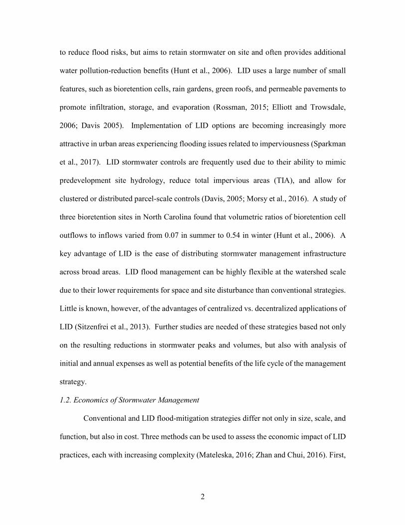
1.1 Hydrologic Effects of Urbanization and Management Strategies
Urbanized watersheds can have a high percent impervious area (PIA) that leads to
increased runoff (Jacobson, 2011; Walsh et al., 2005; Scheuler, 1994). They also tend to
have an extensive network of storm sewers (SS) that accelerates the arrival of flood waves.
Combined, PIA and SS systems can greatly multiply peak discharge in urban watersheds
and accelerate stormflow arrival times (Leopold, 1968; Putnam, 1972; Bohman, 1992;
Meierdiercks et al., 2010).
Stormwater management planning can best mitigate these hydrologic changes if
flows through the physical infrastructure and processes are well understood, which can be
assisted by the use of hydrologic simulations. Stormwater designs to reduce flood risks in
urbanized watersheds typically can be classified as conventional or low impact
development. Conventional stormwater management techniques emphasize the removal of
water from developed sites via concentrated flows in ditches, gutters or storm sewers to
local storage facilities, such as retention or detention ponds, that delay the release to
streams (Wanielista and Yousef 1993). These stormwater-mitigation strategies focus
primarily on reduction of peak flow rates for larger storm events (Sparkman et al., 2017).
Due to the cost and scale of structures, conventional stormwater design is inherently
centralized. Low impact development (LID), also known as green infrastructure, green
engineering, spatially distributed, or source-control stormwater management, is also used
2
to reduce flood risks, but aims to retain stormwater on site and often provides additional
water pollution-reduction benefits (Hunt et al., 2006). LID uses a large number of small
features, such as bioretention cells, rain gardens, green roofs, and permeable pavements to
promote infiltration, storage, and evaporation (Rossman, 2015; Elliott and Trowsdale,
2006; Davis 2005). Implementation of LID options are becoming increasingly more
attractive in urban areas experiencing flooding issues related to imperviousness (Sparkman
et al., 2017). LID stormwater controls are frequently used due to their ability to mimic
predevelopment site hydrology, reduce total impervious areas (TIA), and allow for
clustered or distributed parcel-scale controls (Davis, 2005; Morsy et al., 2016). A study of
three bioretention sites in North Carolina found that volumetric ratios of bioretention cell
outflows to inflows varied from 0.07 in summer to 0.54 in winter (Hunt et al., 2006). A
key advantage of LID is the ease of distributing stormwater management infrastructure
across broad areas. LID flood management can be highly flexible at the watershed scale
due to their lower requirements for space and site disturbance than conventional strategies.
Little is known, however, of the advantages of centralized vs. decentralized applications of
LID (Sitzenfrei et al., 2013). Further studies are needed of these strategies based not only
on the resulting reductions in stormwater peaks and volumes, but also with analysis of
initial and annual expenses as well as potential benefits of the life cycle of the management
strategy.
1.2. Economics of Stormwater Management
Conventional and LID flood-mitigation strategies differ not only in size, scale, and
function, but also in cost. Three methods can be used to assess the economic impact of LID
practices, each with increasing complexity (Mateleska, 2016; Zhan and Chui, 2016). First,

3
a simple cost comparison can be made between the initial construction costs of differing
methods of LID treatment. Second, a life-cycle cost (LCC) analysis can be completed,
adding another dimension of costs throughout the life of the stormwater control (Chui et
al., 2016; Houle et al., 2013). Life-cycle costs (LCC) can be calculated starting with initial
costs including land acquisition, design and construction, and annual operation and
maintenance (O&M) costs over the expected life of the management strategy (Mateleska,
2016; Chui et al., 2015;). Mateleska (2016) found that detention pond design and
construction had a lower unit storage cost ($/m3) than bioretention, $240.04 and $547.70
respectively, however bioretention cells were estimated to require 20.6% less annual
investment related to O&M. Houle et al. (2013) reported similar results in a study reporting
annual costs and required maintenance hours, with bioretention providing a 17.7%
reduction in annual O&M costs over the course of their life-cycle. Benefit-cost analysis
(BCA) provides a third means of comparing economic efficiency of management
strategies, considering all relevant LCC and net life-cycle benefits (LCB), including
environmental and social non-market benefits. While LCC analysis provides a more
realistic long term understanding of stormwater management costs than a basic comparison
of initial investment costs, a full BCA can provide a more accurate assessment of
differences in total cost over the life cycle of a management strategy (Zhan and Chui, 2016;
EPA, 2013). Typical life-cycles of stormwater controls range from 20-30 years, although
these types of analysis often consider a longer period of 50 years or more (Zhan and Chui,
2016; Veseley, 2005). CBA can be significantly more complex than LCC analysis because
many of these benefits do not have a direct economic value attached to them and therefore
value must be inferred through non-market valuation strategies. Although both

4
conventional and LID strategies provide direct economic benefits from runoff and
discharge quantity reductions as well as various water quality benefits, LID provides more
extensive environmental and societal benefits than conventional strategies including
improved air quality, CO2 sequestration, and thermal benefits from reduction of the urban
heat island effect, as well as benefits to society such as improved citizen health and
aesthetic benefits (Zhan et al., 2016; EPA 2013; Veseley, 2005). Environmental benefits
can often be quantified through assessment of potential savings from avoided
consequences, while social benefits must be inferred from contingent valuation strategies
in which willingness to pay (WTP) for the infrastructure in question is evaluated by
observing the preferences of an individual or group, either directly stated or ‘observed’
preferences (Zhan and Chui, 2016). A study based on contingent valuation surveys,
experimental real estate negotiations, and spatial hedonic price methods found that
individuals revealed an increased WTP for LID (Bowman et al., 2012). Individuals with
prior knowledge of LID also showed higher WTP than those who were unfamiliar. This is
an important advantage of LID, as public use of LID practices such as disconnecting
rooftop runoff or the use of rain barrels can increase storage within a watershed without
adding additional government and institutional expenses. Evaluation of the LCC and LCB
of stormwater control must also include a discount rate and an inflation rate in order to
observe these monetary values in the context of future value (FV). While there is no agreed
upon value for these rates, previous research has used discount rates from 3.5 – 4.25% and
inflation rates from 2 – 5% (Zhan and Chui, 2016; EPA, 2013; Veseley, 2005). While the
management scenarios designed for this study based on initial design and construction

5
costs per unit of storage ($/m3), a review of the economic benefits of LID revealed through
BCA addresses the potential long-term efficiency of these strategies.
1.3. Hydrologic (Rainfall/Runoff) Modeling With SWMM
Rainfall-runoff models can be used to simulate hydrologic responses, such as
infiltration, surface runoff, and channel and pipe flow to changes in land use or stormwater
treatment practices. These models typically incorporate observed rainfall data, land use,
and geospatial characteristics, as well as conveyance relationships between open channels,
culverts, and floodplains. They are calibrated and validated with stream flow data. The
models provide a tool that can be used to test scenarios of changes to the hydrologic system.
One such model is the EPA’s Storm Water Management Model (SWMM) (Rossman,
2015), which is an open-source model intended for urbanized watersheds. First developed
in 1971 and now on its fifth version, SWMM is a dynamic rainfall-runoff simulation model
capable of single-event or continuous simulations of water quantity and quality (Rossman,
2015; Barco et al., 2008). SWMM routes runoff for subcatchments with storm drains,
combined sewers, and natural drainage through a network of pipes, channels, and
storage/treatment units (Rossman, 2015; Barco 2008). The SWMM simulates three
primary processes: stormwater infiltration, surface runoff, and flow routing. The latest
versions of SWMM (e.g., version 5.1.012) can model hydrologic performance of typical
conventional and LID controls with varying sizes, coverage, and geographic distributions.
The LID controls include, but are not limited to, bioretention and green roofs (Rossman,
2015).
The primary applications of SWMM, as related to this research, include simulations
of runoff volumes and discharge, that can be used for planning, analysis, and design of

6
stormwater drainage systems. The SWMM has the ability to simulate runoff volumes and
timing as stormwater flows through conventional detention infrastructure and eight
different LID configurations, including bioretention cells, green roofs, and permeable
pavements (Rossman, 2015). The model can also account for numerous hydrologic
processes and water budgeting including precipitation time series, runoff storage,
infiltration, evapotranspiration, and interaction with groundwater layers and interflow
(Rossman, 2015). Three flow routing methods can be used for SWMM: steady flow,
kinematic wave, or, where the purpose is for event-based storm events such as this study,
dynamic wave, which accounts for backwater effects (Rossman, 2015). Once calibrated to
observed rainfall and stream-flow data, SWMM can simulate the implementation of virtual
conventional storage units or LID scenarios in order to evaluate their effectiveness in
reducing surface runoff depth and peak discharge. Modeling flood-control implementation
scenarios of varying type, size, and spatial location can accurately determine which
stormwater management scenarios are most effective. Rosa et al. (2015) compared the
accuracy of calibrated and uncalibrated SWMM models that incorporate LID controls and
found that uncalibrated models underpredicted key runoff components by as much as 80%.
In contrast, calibrated models produced results within 12% of observed values.
The objectives of this study are to (1) observe and compare the effectiveness of
both conventional and LID strategies in reducing peak flow for moderate-magnitude storms
in a small, highly urbanized watershed, (2) observe the effectiveness of LID in reducing
total runoff volume (locally) within the test subcatchment of implementation (3) observe
and compare the effectiveness of LID strategies when implemented in different patterns in
the watershed, both localized (lumped) and distributed, and (4) observe SWMM results in
7
reference to the economic effectiveness of conventional and LID strategies. A series of
simple hypotheses are presented to structure objective tests for objectives one and two
(Table 1.1). These hypotheses will be applied independently at each of the two stream
gauges.
Table 1.1. Hypotheses regarding stormwater management scenarios for moderate-
magnitude storms at given levels of investment
1. Conventional vs LID
H1A LID reduces peak discharges more than conventional management practices.
H1B LID reduces local subcatchment runoff volume.
2. Spatial Patterns of LID
H2 LID grouped in the most urbanized sub-basin is more effective in
reducing peak discharge than LID distributed across multiple sub-basins.
8
CHAPTER 2
METHODS
2.1 Study Area
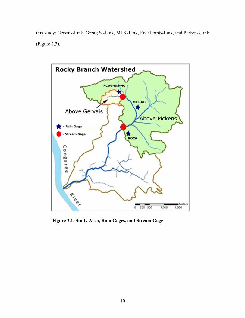
Rocky Branch Watershed (RBW) is contained within an area of roughly 10.3km2
and includes 14.5 km of open stream channels that flow into the Congaree River (Figure
2.1). The RBW contains most of the University of South Carolina campus, much of the
downtown Columbia central business district, the Five Points Commercial District, and
several old residential neighborhoods. With an imperviousness of 49%, the dominant land
use in RBW is developed land of high, medium, and low intensity (McCormick Taylor,
2016). RBW falls entirely within the Sandhills ecoregion and physiographic province with
topographically variable Cretaceous-age marine and aeolian sand (Sweezy et al., 2016).
The high sand content of soils results in high contrasts in infiltration rates and runoff
generation between impervious and pervious surfaces. Intense urban development over the
course of the past century left RBW subject to extreme stormwater and water quality issues
based on high longitudinal channel connectivity, low latitudinal floodplain connectivity,
lack of open channel area, upstream imperviousness, and an absence of stormwater
management (McCormick Taylor, 2016). The RBW demonstrates the increase in flood
risk that often accompanies urbanization, as increased PIA and SS densities in the
watershed have generated frequent flood events and water degradation. The area simulated
in this study is the Pickens Basin in the upper RBW and the Gervais
9
Sub-basin nested within the Pickens Basin. Three rain gages provide data for the
SWMM and two streamflow gages were used for calibration and validation.
An assessment for the City of Columbia (hereafter the Assessment) of the current
condition of RBW utilized field mapping, hydrologic and hydraulic analysis, and GIS-
based sub-watershed characterizations (McCormick Taylor, 2016). It subdivided RBW
into 11 sub-watersheds as proposed by the Rocky Branch Watershed (Figure 2.2). This
study refers to the total area of the upper watershed contributing to the Above Pickens gage,
referred to as the Above Pickens Basin (Figure 2.1). Contained within this area are the
Gregg Street (GS), Martin Luther King Park (MLK), Devine Blossom (DB), Hollywood-
Rose Hill (HRH), and a portion of the University Hill (UH) subwatersheds. The
Assessment made recommendations for watershed-restoration projects including five
flood-water detention areas and thirty-two potential LID projects. Ultimately, their
recommendations prioritized potential storm-water management projects for these areas
using a cumulative ranking index system derived from potential reductions in peak
discharge, total runoff, and unit runoff for the regional 2-year flood. The hydrologic
analysis for the assessment was based largely on a SWMM model developed by KCI
Technologies which was the initial basis for the model used in this study. The 11 sub-
watersheds were further subdivided into sixty subcatchments in the SWMM model in order
to produce a semi-distributed model (McCormick Taylor, 2016). This study is focused on
the portion of the model above the Pickens Street streamflow gage, which includes 27
subcatchments. Of these subcatchments, five are used as locations for modeled stormwater
controls: GS-1, GS-2, GS-3, MLK-9, and UH-3 (Figure 2.3). SWMM defines sections of
open channel or SS conduits as ‘links,’ and peak flows within five links are observed in
10
this study: Gervais-Link, Gregg St-Link, MLK-Link, Five Points-Link, and Pickens-Link
(Figure 2.3).
Figure 2.1. Study Area, Rain Gages, and Stream Gage

11
Figure 2.2. McCormick Taylor (2016) subwatershed delineation. The area
observed for this study includes GS, MLK, UH, DB, and HRH

12
Figure 2.3. Upper RBW (above bold line) including 5 test subcatchments
for stormwater controls and computation of runoff volumes and 5 test links
examined for Qpk
A previous study utilized a SWMM model in RBW to model the effectiveness of
LID controls, specifically rain gardens (Morsy et al., 2016). While incorporating
parameters similar to the model developed in this study, the focus of that study was on
flow-stage reduction based on different runoff-routing scenarios and focused on how much
runoff must be diverted to proposed LID controls in order to account for runoff from
various precipitation frequencies (Morsy et al., 2016). The study reported here compares
13
the mitigation of stormwater resulting from the implementation of conventional and LID
management practices.
2.2. Model Overview and Data Preparation
Initial model parameter estimation was based on existing literature, previous model
settings, and model defaults. The GREEN-AMPT infiltration was adopted from previous
versions of the model for RBW developed by KCI. The SS network was mapped by the
City of Columbia (CoC) and imported the existing SWMM by KCI (McCormick Taylor,
2016). Soil characteristics were chosen based on SURGO digital data (USDA, 1978;
1994). The dynamic wave model was selected for flow routing because it accounts for
channel storage, backwater effects, entrance and exit losses, flow reversals, and pressurized
flow, all of which are known to occur during floods in RBW. Spatial data for RBW
subcatchments, including drainage area, slope, and percent impervious area (PIA), were
analyzed through geographic information system (GIS) procedures and used to update the
model.
GREEN-AMPT parameters, such as suction head and hydraulic conductivity, were
adjusted based on values appropriate for loamy sand, the dominant soil type in RBW
(Rossman, 2015; Rawls and Brackensiek, 1993; Rawls et al., 1983;). Ranges for detention
storage and Manning’s roughness for overland flow were based on values cited in the 2016
SWMM Manual and other standard hydrology sources (Rossman, 2015; McCuen, 1996;
ASCE, 1983; 1992). Stream channel and conduit profiles, dimensions, and roughness
(Manning’s n) were adopted from the existing model, although some open channel
roughness values (Manning’s n) were adjusted to more realistic values, and an updated
channel profile was added to the model for the ‘Above Gervais’ calibration point. The

14
SWMM model used in this study utilized 5-minute rainfall data from three gages. Rain
gage RCWINDS-HQ was operated by the Richland County Weather Information Network
Data System and rain gages MLK-RG and ROCA were operated by Woolpert Inc., LLC
for the CoC. The initial model was calibrated to stage data at Pickens and was recalibrated
for this study using flow data from two locations: stage data (m) at the ‘Above Gervais’
gage and discharge data at the ‘Above Pickens’ gage (Figure 2.1). The stage data at
Gervais were measured at two-minute intervals using a Solinst barometrically corrected
level logger, and converted to five-minute intervals for model assessments. The discharge
data at Pickens were collected by Woolpert Inc., LLC for the CoC using an acoustic
Doppler current profiler (ADCP) at five-minute intervals (Figure 2.4).
Observed storm events for calibration and modeling were screened and selected for
the study period of July 1, 2016 to February 1, 2018 at the RCWINDS-HQ and ROCA
rainfall stations, the closest locations to the streamflow gages used for calibration at Above
Gervais and Above Pickens, respectively. Precipitation events were screened visually and
eliminated if rainfall was highly variable in time or between gage locations to avoid multi-
modal hydrographs and spatially variate intensities. Events were discarded with discharges
exceeding 15 m3/s at the Above Pickens gage due to observed difficulties with SWMM
computation of overbank discharges. Precipitation durations for chosen storms ranged
from 20 to 105 minutes, and precipitation depths ranged from 7.5 – 20 mm. Selected
stormflow durations were determined using a factor of 5.4 times the time-to-peak following
the time of peak discharge, calculated based on the end of stormflow for the storm event
on May 29, 2017, a 35-min, 14 mm rainfall at HQ rain gage, resulting in the peak stage of
0.802 m at Gervais and the peak discharge of 9.97 m3/s at Pickens. Six storm events were

15
selected, three for calibration and three for validation (Table 2.1). The 5/29/2017 event was
selected as the base storm for scenario modeling due to its moderate-magnitude intensity
and short duration (Figure 2.5).
Figure 2.4. SWMM Model Layout including all subcatchments, links,
and nodes. Only the upper portion of the model above Pickens was
calibrated and used for this study

16
Table 2.1. Observed Storm Events
Event Code Event Date Duration Cumulative
Rainfall Depth
Rainfall
Intensity
ROCA
Qpk
(m3/s)
C1 5/22/2017 105 20 4.4 1.7
C2 5/29/2017 40 19.3 9.7 10.0
C3 8/13/2017 55 21 7.6 14.5
V1 5/24/2017 75 12 3.7 9.6
V2 7/25/2017 35 14 14.0 7.8 V3 10/16/2017 35 14 8.0 8.3
Figure 2.5. Observed rainfall at the ROCA rain gage and discharge at the Above
Pickens stream gage for the base storm 5/29/2017
2.3. Model Sensitivity
Sensitivity analysis was performed to asses which parameter changes would be
most effective in minimizing differences between simulated and observed concentrated
stormflow values during calibration (Rosa et al., 2015). Parameters were adjusted over a
0.000
0.200
0.400
0.600
0.800
1.000
1.200
1.400
0
2
4
6
8
10
12
0 0.5 1 1.5 2 2.5 3 3.5
Ra
infa
ll (
mm
)
Dis
cha
rge
(m
3/s
)
Elapsed Time (Hours)
May 29, 2017 Storm Event
ROCA Rainfall Pickens-Link Q
17
range of ±50% of their original value with all other parameters remaining constant and the
resulting changes in peak flow were noted at calibration locations. Relative sensitivity was
computed by the method used by Rosa et al. (2015):
Sensitivity=(∂R/∂P)(P/R) (1)
where ∂R is the difference between the original and new model output, ∂P is the difference
between the original and adjusted parameter value, R is the original model output, and P is
the original value of the chosen parameter of interest (Rosa et al., 2015; James and Burges,
1982). Green-Ampt infiltration parameters have been used as sensitive parameters for
calibration, as well as Manning’s n (roughness), saturated hydraulic conductivity, and
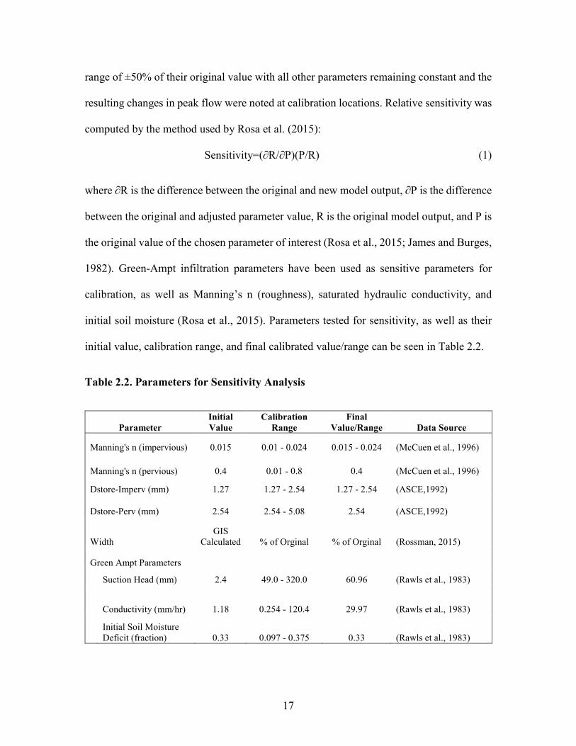
initial soil moisture (Rosa et al., 2015). Parameters tested for sensitivity, as well as their
initial value, calibration range, and final calibrated value/range can be seen in Table 2.2.
Table 2.2. Parameters for Sensitivity Analysis
Parameter
Initial
Value
Calibration
Range
Final
Value/Range Data Source
Manning's n (impervious) 0.015 0.01 - 0.024 0.015 - 0.024 (McCuen et al., 1996)
Manning's n (pervious) 0.4 0.01 - 0.8 0.4 (McCuen et al., 1996)
Dstore-Imperv (mm) 1.27 1.27 - 2.54 1.27 - 2.54 (ASCE,1992)
Dstore-Perv (mm) 2.54 2.54 - 5.08 2.54 (ASCE,1992)
Width GIS
Calculated % of Orginal % of Orginal (Rossman, 2015)
Green Ampt Parameters
Suction Head (mm) 2.4 49.0 - 320.0 60.96 (Rawls et al., 1983)
Conductivity (mm/hr) 1.18 0.254 - 120.4 29.97 (Rawls et al., 1983)
Initial Soil Moisture Deficit (fraction) 0.33 0.097 - 0.375 0.33 (Rawls et al., 1983)
18
2.4. Model Calibration and Validation
Event-based calibration was completed using three of the six events chosen during
storm screening. Sensitive parameters were changed one at a time during calibration until
differences between simulated and observed flows were minimized, or until a limit of the
accepted range of the parameter was reached (Rosa et al., 2015; Morsy et al., 2016).
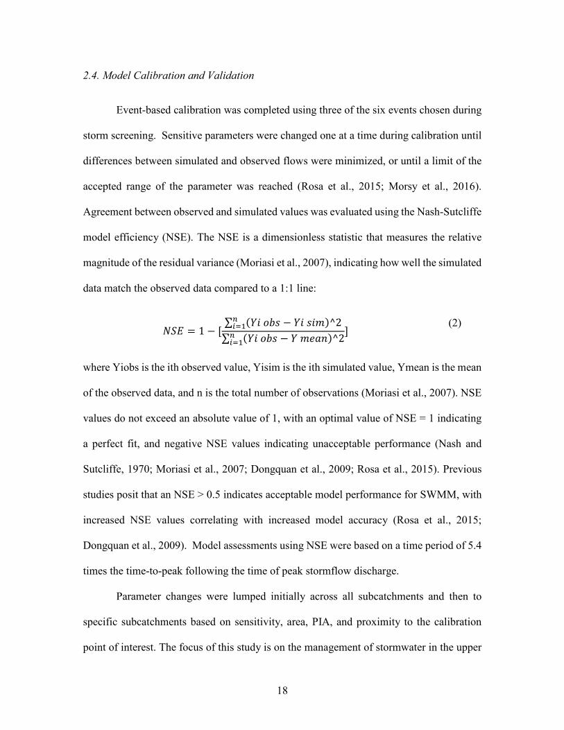
Agreement between observed and simulated values was evaluated using the Nash-Sutcliffe
model efficiency (NSE). The NSE is a dimensionless statistic that measures the relative
magnitude of the residual variance (Moriasi et al., 2007), indicating how well the simulated
data match the observed data compared to a 1:1 line:
��� = 1 − [∑ � �� − � ����^2�
���
∑ � �� − �����^2����
] (2)
where Yiobs is the ith observed value, Yisim is the ith simulated value, Ymean is the mean
of the observed data, and n is the total number of observations (Moriasi et al., 2007). NSE
values do not exceed an absolute value of 1, with an optimal value of NSE = 1 indicating
a perfect fit, and negative NSE values indicating unacceptable performance (Nash and
Sutcliffe, 1970; Moriasi et al., 2007; Dongquan et al., 2009; Rosa et al., 2015). Previous
studies posit that an NSE > 0.5 indicates acceptable model performance for SWMM, with
increased NSE values correlating with increased model accuracy (Rosa et al., 2015;
Dongquan et al., 2009). Model assessments using NSE were based on a time period of 5.4
times the time-to-peak following the time of peak stormflow discharge.
Parameter changes were lumped initially across all subcatchments and then to
specific subcatchments based on sensitivity, area, PIA, and proximity to the calibration
point of interest. The focus of this study is on the management of stormwater in the upper

19
watershed above Pickens, therefore, the model is not considered to be calibrated below this
point.
2.5. Management Scenarios and Scenario Development
Management scenarios were designed to test the hypotheses concerning
comparisons of LID and conventional treatment and geographic locations of treatments.
The conventional and LID configurations were narrowly defined to control comparisons,
but each of those configurations could be modified to substantially change results. For
example, peak discharges under conventional management were highly sensitive to the
outlet structures of detention structures that changed arrival times of flow peaks.
Optimization of outlet structures for the moderate-magnitude flows in this study would not
likely be optimal for larger flows, and optimizing over a large range of flows was beyond
the scope of this study. Management scenarios were broken into a set of tests with varying
locations of virtual stormwater management controls based on recommendations from the
assessment for potential restoration opportunities within RBW (McCormick Taylor 2016).
Although varying somewhat in size and treatment area, all bioretention cell locations were
derived from the assessment. Conversely, placement of only one detention pond—located
at GS-5—was derived from the assessment, as GS-5 was the only catchment with both a
conventional and LID recommendation. Remaining detention pond locations were chosen
based on recommended LID locations for the purpose of direct comparisons. All SWMM
scenarios for this study were modeled using precipitation data from the May 29, 2017
calibration storm, a 40-minute event with rainfall intensities of 8 mm/20 min and 9.7
mm/20 min at RCWINDS-HQ and ROCA, respectively. This storm was selected as the
base storm for modeling due to its relatively high intensities and consistency between

20
intensities at both calibration locations. This study observes modeling results from two
tests shown in Table 2.3.
Table 2.3. Test 1 and 2 Details
Test Details Links Observed for Qpk
Test 1 (T1)
Detention Ponds and bioretention implemented one at a time in GS-5, MLK9, and UH3. Tests H1A and H1B.
T1L1 (GS-5): Gervais Link, Pickens Link T1L2 (MLK-9): MLK-Link, Pickens Link T1L3 (UH-3): Pickens Link
Test 2A (T2A) Localized Scenario; Bioretention implemented at GS-1, GS-2, and GS-3. Tests H2.
Gervais-Link; Gregg St-Link; MLK-Link; Five Points-Link; Pickens-Link
Test 2B (T2B) Distributed Scenario; Bioretention implementd at GS-5, MLK-9, and UH-3. Tests H2.
Gervais-Link; Gregg St-Link; MLK-Link; Five Points-Link; Pickens-Link
Stormwater management Test 1 (T1) was designed to compare the effectiveness of
conventional detention basins to that of bioretention cells (LID) in reducing peak discharge
(m3/s) of concentrated flows within conduit and channel links. Bioretention scenarios were
assessed for effectiveness in reduction of local runoff volume (106 m3), but simulations of
detention ponds were not expected to show changes in runoff volume due to the way in
which the model views the storage unit as a subcatchment outlet node rather than a part of
the subcatchment itself. The configuration and size of detention ponds or bioretention cells
were based on assumptions of initial investment for design and construction costs only,
each modeled separately at three locations for a total of six SWMM runs. Location 1,
Location 2, and Location 3 were at GS-5, MLK-9, and UH-3 respectively (Figure 2.6).

21
Figure 2.6. Test 1 locations and observation links. Each location
models individual stormwater controls. Runoff results are observed
at the test location, and Qpk is observed at the link closest to the test
location as well as the Pickens-Link for all scenarios
Sizing of detention ponds and bioretention cells were based on unit storage costs
($/m3) of $240.04 and $545.70 for detention ponds and bioretention structures,
respectively (Table 2.4) (Mateleska, 2016). Costs of bioretention structures were computed
based on the volumes of their storage areas only, not including void space within the soil
layer or surface ponding depth. These estimates indicate that the initial installation of
bioretention cells cost more than twice that of detention ponds on a dollar-per-volume of

22
storage basis. Each iteration of T1 was performed twice based on initial investment
assumptions, with Investment Level 1 (IL1) and Investment Level 2 (IL2) equaling
$100,000 and $200,000 respectively., Based on this doubling of investment between IL1
and IL2, the second model run in each case had twice the storage volume as the first. For
example, the given unit storage costs, IL1 and IL2 resulted in detention pond storage of
417 m3 and 832 m3 and bioretention cell storage of 183 m3 and 367 m3, respectively.
Changes in Qpk (m3/s) for all Test 1 scenarios are observed at the closest observation link
to the location being tested and at the downstream Pickens-Link, which acts as a control
observation point for all T1 locations. Test 1 also observes changes in total runoff volume
(m3) for bioretention only within the test subcatchment of implementation.
Table 2.4. Unit Prices Per Cubic Meter of Storage in 2016 Dollars (Source:
Mateleska, 2016)
Management Strategy Unit Costs ($/m3) – 2016
Dollars Volume (m3) / $100,000
Detention Pond $240.04 417
Bioretention Cell $545.70 183
Detention ponds were designed in SWMM as basic storage units with a depth/area
relationship defined using the tabular curve method. Subcatchments within the SWMM
model are set up to route all overland flow to an outlet node with no routing between
subcatchments due to drainage divides. For this reason, modeled detention ponds were
designed to function at the outlet node for their respective subcatchments, with pond
inflows conveyed through a conduit to the original outlet node of the subcatchment. Based

23
on a sensitivity analysis, outlet conduits for detention ponds used a 46-cm (18”) outlet pipe
to be small enough to store and delay conveyance of inflows while draining outflows
quickly enough for the pond to have available storage for storm events larger than the one
chosen for this study.
Bioretention cells in SWMM include three vertical layers (Figure 2.7)—a surface
layer where ponding can occur up to a specified height, a soil media layer, and a storage
layer with the option of loss via infiltration, a drain outlet, or both (Rossman, 2010).
Figure 2.7. SWMM representation of
bioretention (Rossman, 2010)
Bioretention cell parameters were selected largely based on existing literature (Table 2.5)
(Lucas, 2005; Rossman, 2010; 2015). Storage capacity was calculated based on void space
within the storage layer and did not include the surface or soil layers. The storage layer was
assumed to have a depth of 1 m and a void ratio of 0.75, resulting in an area of 245 m2 at
the $100,000 investment level. SWMM allows for LID to be designed separately and then
24
applied to the desired subcatchment(s), with the ability to apply multiple identical units to
the same subcatchment. For this reason, a bioretention cell design based on the assumed
$100,000 initial investment was treated as the base unit, and a doubling of assumed
investment level for IL2 was represented by an application of an additional identical unit,
therefore doubling the storage. Bioretention cell drains were positioned 600 mm from the
bottom of the bioretention cells so infiltration is the primary means of storage loss and
drainage to the SS network occurs only for larger events where LID storage exceeds 60%
of capacity. The proportion of sheet flow from impervious surfaces that flows into the
bioretention cell was set at 25%, based on a sensitivity and optimization to reduce runoff
and Qpk while leaving storage available for larger storms.
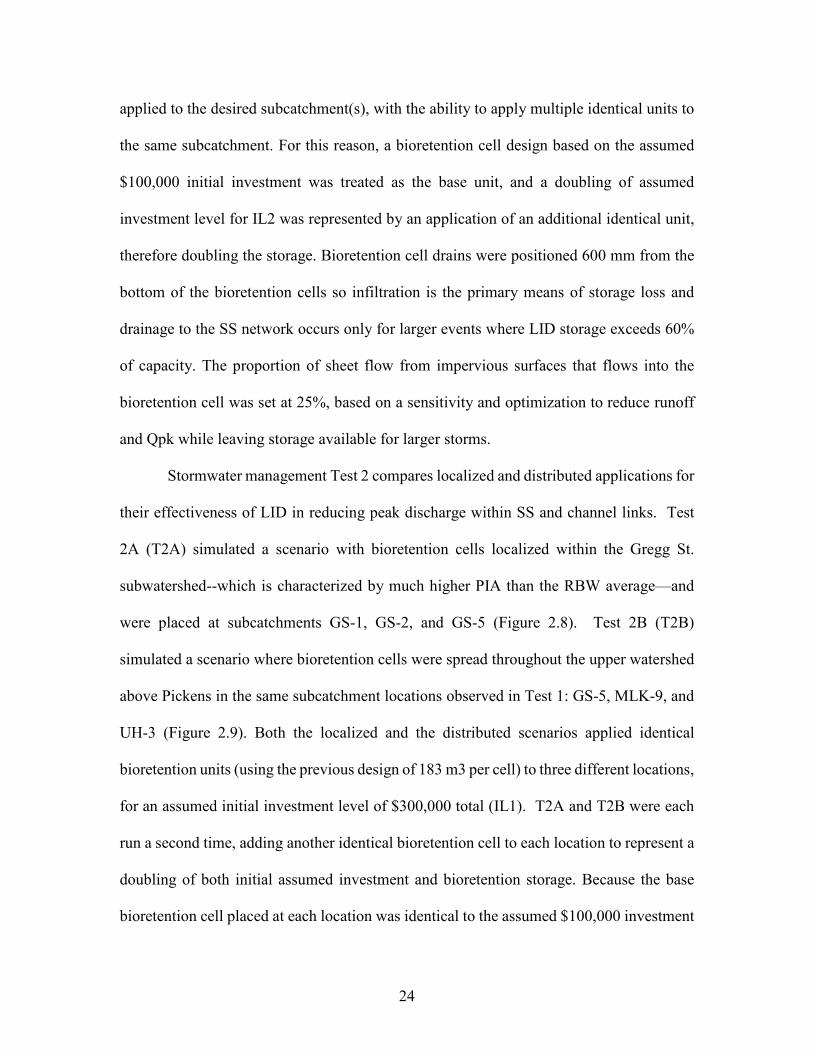
Stormwater management Test 2 compares localized and distributed applications for
their effectiveness of LID in reducing peak discharge within SS and channel links. Test
2A (T2A) simulated a scenario with bioretention cells localized within the Gregg St.
subwatershed--which is characterized by much higher PIA than the RBW average—and
were placed at subcatchments GS-1, GS-2, and GS-5 (Figure 2.8). Test 2B (T2B)
simulated a scenario where bioretention cells were spread throughout the upper watershed
above Pickens in the same subcatchment locations observed in Test 1: GS-5, MLK-9, and
UH-3 (Figure 2.9). Both the localized and the distributed scenarios applied identical
bioretention units (using the previous design of 183 m3 per cell) to three different locations,
for an assumed initial investment level of $300,000 total (IL1). T2A and T2B were each
run a second time, adding another identical bioretention cell to each location to represent a
doubling of both initial assumed investment and bioretention storage. Because the base
bioretention cell placed at each location was identical to the assumed $100,000 investment

25
from T1, Test 2 observed initial investment levels of $300,000 (IL1) and $600,000 (IL2).
Both the localized and distributed scenarios modeled the cumulative effects of
implementing three cells at once on Qpk (m3s/) at the five observation links shown in
Figures 2.8 and 2.9, with emphasis on Qpk at the downstream Pickens-Link.
Table 2.5. SWMM Bioretention Parameters (Source: Lucas, 2005; Rossman, 2010;
2015)
Surface Layer Value Soil Layer Value Storage Layer Value Drain Value
Berm Height (mm)
450 Thickness (mm) 750 Thickness (mm)
1000 Flow Coefficient
1
Vegetative Volume (Fraction)
0.1 Porosity (volume fraction)
0.5 Void Ratio (voids/solids)
0.75 Flow Exponent
0.5
Surface Roughness (Manning’s n)
0.24 Field Capacity (volume fraction)
0.105 Infiltration Rate (mm/hr)
12.7 Offset Height (mm)
600
Surface Slope (percent)
1 Wilting Point (volume fraction)
0.047 Clogging Factor
0
Conductivity (mm/hr)
29.97
Conductivity Slope
10
Suction Head (mm)
60.97

26
Figure 2.8. Test 2A (Localized) bioretention locations and observation links

27
Figure 2.9. Test 2B bioretention locations and observation links
28
CHAPTER 3
RESULTS
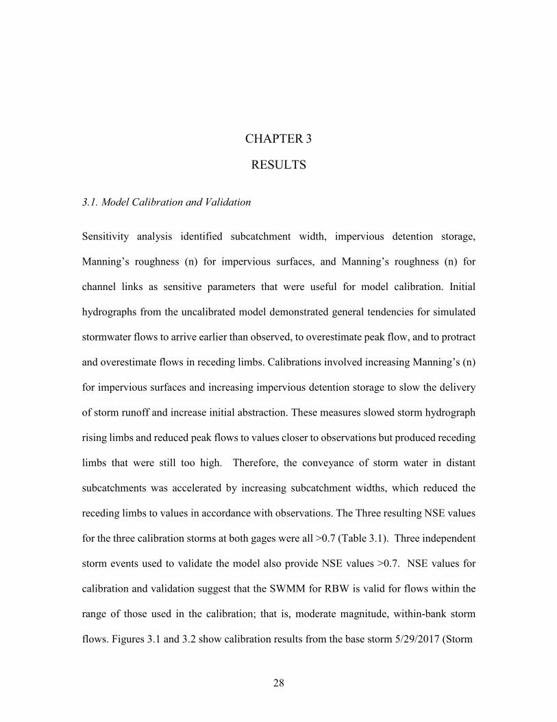
3.1. Model Calibration and Validation
Sensitivity analysis identified subcatchment width, impervious detention storage,
Manning’s roughness (n) for impervious surfaces, and Manning’s roughness (n) for
channel links as sensitive parameters that were useful for model calibration. Initial
hydrographs from the uncalibrated model demonstrated general tendencies for simulated
stormwater flows to arrive earlier than observed, to overestimate peak flow, and to protract
and overestimate flows in receding limbs. Calibrations involved increasing Manning’s (n)
for impervious surfaces and increasing impervious detention storage to slow the delivery
of storm runoff and increase initial abstraction. These measures slowed storm hydrograph
rising limbs and reduced peak flows to values closer to observations but produced receding
limbs that were still too high. Therefore, the conveyance of storm water in distant
subcatchments was accelerated by increasing subcatchment widths, which reduced the
receding limbs to values in accordance with observations. The Three resulting NSE values
for the three calibration storms at both gages were all >0.7 (Table 3.1). Three independent
storm events used to validate the model also provide NSE values >0.7. NSE values for
calibration and validation suggest that the SWMM for RBW is valid for flows within the
range of those used in the calibration; that is, moderate magnitude, within-bank storm
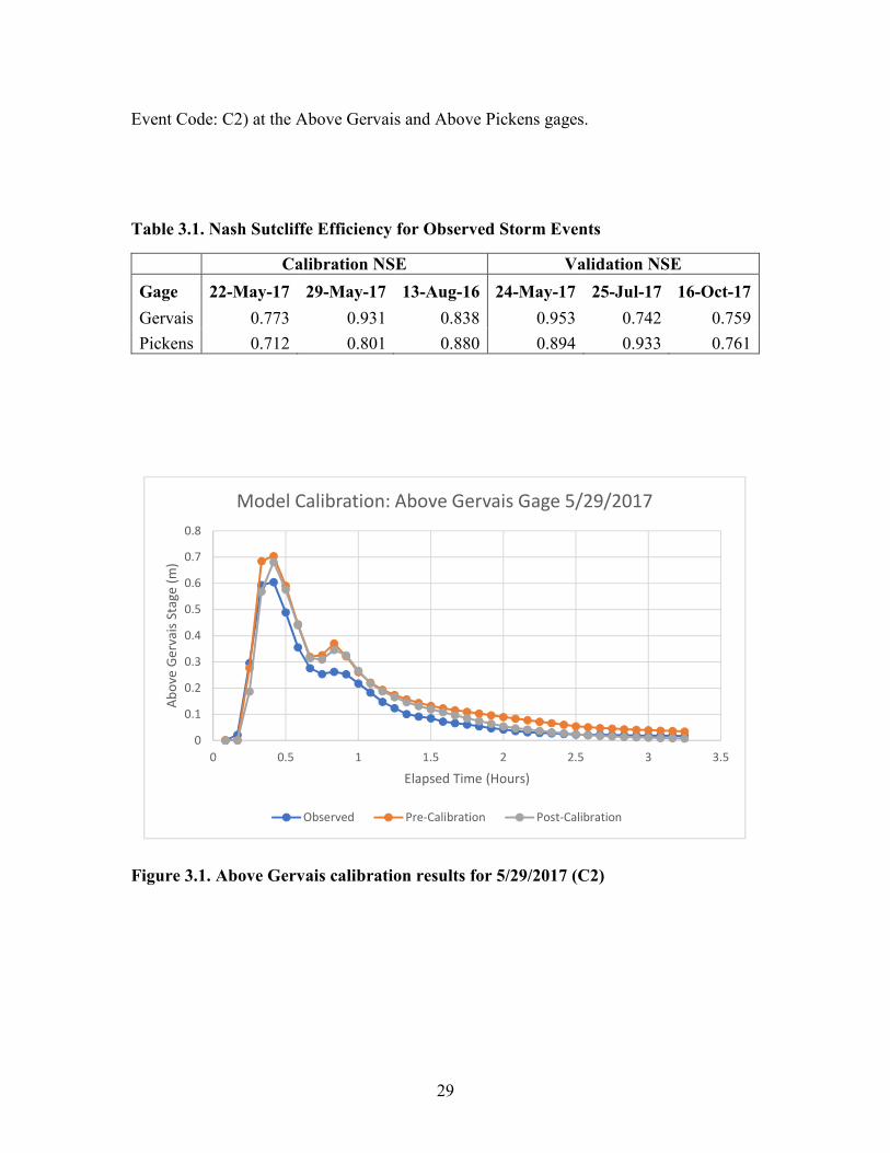
flows. Figures 3.1 and 3.2 show calibration results from the base storm 5/29/2017 (Storm
29
Event Code: C2) at the Above Gervais and Above Pickens gages.
Table 3.1. Nash Sutcliffe Efficiency for Observed Storm Events
Calibration NSE Validation NSE
Gage 22-May-17 29-May-17 13-Aug-16 24-May-17 25-Jul-17 16-Oct-17
Gervais 0.773 0.931 0.838 0.953 0.742 0.759
Pickens 0.712 0.801 0.880 0.894 0.933 0.761
Figure 3.1. Above Gervais calibration results for 5/29/2017 (C2)
0
0.1
0.2
0.3
0.4
0.5
0.6
0.7
0.8
0 0.5 1 1.5 2 2.5 3 3.5
Ab
ove
Ge
rva
is S
tag
e (
m)
Elapsed Time (Hours)
Model Calibration: Above Gervais Gage 5/29/2017
Observed Pre-Calibration Post-Calibration
30
Figure 3.2. Above Pickens calibration results for 5/29/2017 (C2)
3.2. Test 1 Stormflow Reductions: Conventional and LID Strategies
Each of the Test 1 scenarios simulate a single stormwater management type
concentrated in a single sub-basin. Peak discharge (Qpk) results were measured from
specific channel or conduit links in the SWMM and represent all contributing flows above
that point, which were reported as change in Qpk (m3/s), as well as percent change from
initial values (Table 3.2). When management treatments are isolated, both detention ponds
and bioretention cells influenced Qpk, although the effectiveness in stormwater reductions
differed between scenarios. Both types of management were most effective when
positioned at Location 1 (GS-5). The largest reductions were locally at the Gervais-Link,
where detention pond Qpk percent reductions were -11.2% and -17.4% for Investment
Level 1 (IL1) and Investment Level 2 (IL2).
0
2
4
6
8
10
12
14
0 0.5 1 1.5 2 2.5 3 3.5
Ab
ove
Pic
ke
ns
Dis
cha
rge
(m
3/s
)
Elapsed Time (Hours)
Model Calibration: Above Pickens Gage 5/29/2017
Observed Pre-Calibration Post-Calibration

31
Table 3.2. Test 1 Change in Peak Discharge Rates
Investment Level 1
(IL1): $100,000 Investment Level 2 (IL2): $200,000
Test Location
Management Control
Observation Link
Change in Qpk (m3/s)
% Change
Change in Qpk (m3/s)
% Change
Test Location 1 (T1L1): GS-5 Detention Pond
Gervais-Link -0.26 -11.2% -0.40 -17.4%
Pickens-Link -0.17 -1.5% -0.23 -2.0%
Bioretention
Gervais-Link -0.14 -6.0% -0.14 -6.0%
Pickens-Link -0.07 -0.6% -0.09 -0.7%
Test Location 2 (T1L2): MLK-9 Detention Pond MLK-Link 0.12 2.5% 0.07 1.3%
Pickens-Link 0.01 0.1% -0.04 -0.3%
Bioretention MLK-Link -0.01 -0.2% -0.04 -0.9%
Pickens-Link -0.04 -0.4% -0.06 -0.6%
Test Location 3 (T1L3): UH-3 Detention Pond
Pickens-Link 0.15 1.3% 0.13 1.2%
Bioretention
Pickens-Link 0.00 0.0% 0.01 0.1%
This scenario of detention pond placement at GS-5 also produced the greatest reductions
in Qpk and percent change in Qpk downstream at the Pickens gage, although reductions
were still modest ranging from -1.5% to -2% for IL1 and IL2. In comparison, bioretention
Qpk reductions at the Gervais-Link were only 6% at both investment levels. The lack of

32
increased reduction with a doubling in bioretention volume suggests that the increased
storage capacity at that one subcatchment based on a doubled initial investment is not
needed for the moderate magnitude storms examined in this study. This effect is only seen
with the increase in investment level at GS-5, likely due to its lower drainage area
compared to Location 2 (MLK-9) and Location 3 (UH-3). Implementation of detention
ponds within the Gervais subcatchment led to Qpk reductions at Pickens that were more
than twice the reductions achieved by bioretention at both investment levels, with the
maximum reduction of 2% resulting from IL2.
Test 1 simulations of detention ponds at Location 2 (MLK) generally failed to
produce reductions in Qpk at both the MLK-Link and Pickens-Link. The only reduction
occurs downstream at Pickens at IL2. In every other case, detention pond implementation
increased Qpk within the MLK-Link by 2.5% and 1.3%, respectively, at IL1 and IL2. In
either case, the pond is never more than 53% filled, suggesting that the limitation is in the
design of the pond. This increased Q, however, reveals a danger with conventional storage
methods that may temporarily store flows and release them later when stormwater is
arriving from distant catchments, adding to the peak discharge. Bioretention cells at
Location 2 barely reduced flow rates at the MLK-Link and Pickens-Link at IL1, although
at IL2 the local reduction at MLK of 0.2% was smaller than the downstream reduction at
Pickens of 0.4%. At IL2 the Qpk reduction at the MLK-Link increased to 0.9% (the largest
of any Location 2 percent Qpk reduction) but percent reductions downstream at the
Pickens-Link were only 0.6%.
Simulations at Location 3 (UH-3) showed that neither detention pond nor
bioretention controls were highly effective in reducing Qpk at the Pickens-Link. Detention

33
ponds caused an increase of ~1.2% in Qpk at both investment levels. In contrast to Location
2 (MLK) detention pond results, Location 3 (UH-3) pond results suggest a need for greater
storage capacity in order to be efficient, as ponds were filled to 88% and 100% capacity,
for IL1 and IL2 respectively. Location 3 bioretention reductions were the least effective
for both total runoff volume and Qpk and were negligible at both investment levels.
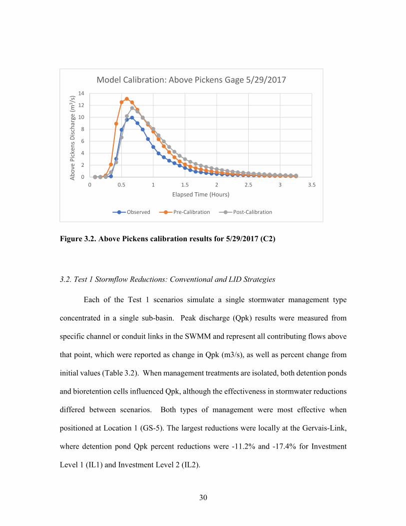
Results from all three of the Test 1 location scenarios show that the local and
downstream discharge or percentage reductions for both detention ponds and bioretention
structures are greatest when implemented at Location 1 (GS-5) and designed based on an
assumed $200,000 initial investment (Figure 3.3 and 3.4). This may be explained by its
higher PIA or lower drainage area and therefore total runoff volume as compared to both
Location 2 (MLK-9) and Location 3 (UH-3). Although changing the location, type of
treatment, or additional allocations had substantial local effects under Test 1 scenarios, the
relatively small amount of variation in peak discharge responses at Pickens suggests that
the effectiveness of the different scenarios in generating reductions in Qpk downstream are
limited.
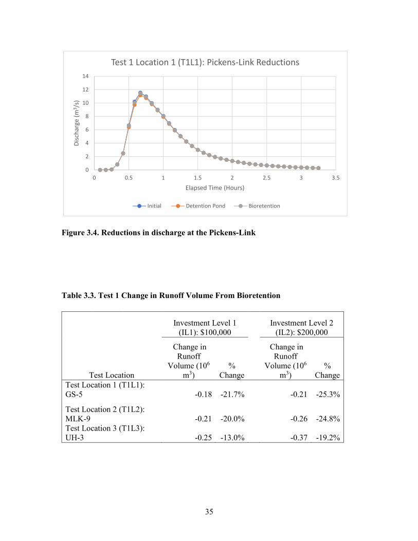
Test 1 simulations of bioretention cells show local reductions in runoff volume
(106 m3) at all three locations and these reductions increase when doubling the assumed
initial investment from IL1 to IL2 (Table 3.3). Percent reductions were greatest at GS-5
for both investment levels, with reductions of 21.7% and 25.3%, respectively, although
greater volumetric and similar percent reductions were achieved with the MLK scenarios.
Simulations of bioretention Location 3 (UH-3) showed the lowest percent reduction in
total runoff volume, with reductions within the subcatchment of 13% at the IL1 and
19.2% at IL2, although these reductions were associated with the greatest volumetric

34
reductions in Qpk (-0.25 to -0.37 m3/s). Simulations of detention ponds did not show
changes in runoff volume due to the way in which they are designed within the SWMM.
For this reason, the 0% reductions in runoff volume from detention ponds were omitted
and not analyzed further.
Figure 3.3. Reductions in discharge at the Gervais-Link
0
0.5
1
1.5
2
2.5
0 0.5 1 1.5 2 2.5 3 3.5
Dis
cha
rge
(m
3/s
)
Elapsed Time (Hours)
Test 1 Location 1 (T1L1): Gervais-Link Reductions
Initial Detention Pond Bioretention
35
Figure 3.4. Reductions in discharge at the Pickens-Link
Table 3.3. Test 1 Change in Runoff Volume From Bioretention
Investment Level 1
(IL1): $100,000 Investment Level 2
(IL2): $200,000
Test Location
Change in Runoff
Volume (106 m3)
% Change
Change in Runoff
Volume (106 m3)
% Change
Test Location 1 (T1L1): GS-5 -0.18 -21.7% -0.21 -25.3%
Test Location 2 (T1L2): MLK-9 -0.21 -20.0% -0.26 -24.8% Test Location 3 (T1L3): UH-3 -0.25 -13.0% -0.37 -19.2%
0
2
4
6
8
10
12
14
0 0.5 1 1.5 2 2.5 3 3.5
Dis
cha
rge
(m
3/s
)
Elapsed Time (Hours)
Test 1 Location 1 (T1L1): Pickens-Link Reductions
Initial Detention Pond Bioretention

36
3.3. Test 2 Stormflow Reductions: Localized and Distributed LID
Test 2 scenarios group LID stormwater management treatments in subcatchments
to compare localized (Test 2A) versus distributed (Test 2B) bioretention approaches.
Resulting Qpk values were observed at five channel or conduit links within the upper
watershed, each representing flow from all contributing links above (Table 3.4).
Table 3.4. Test 2 Change in Peak Discharge Rates
Investment Level 1
(IL1): $300,000 Investment Level 2 (IL2):
$600,000
Scenario Change in Qpk (m3/s)
% Change
Change in Qpk (m3/s) % Change
LOCALIZED (GS-1, GS-2, and GS-5)
Conduit/Channel
Gervais -0.14 -6.0% -0.14 -6.0%
Gregg St -0.52 -13.7% -0.55 -14.5%
MLK 0.00 0.0% 0.00 0.0%
Five Points -0.36 -5.5% -0.37 -5.7%
Pickens -0.27 -2.4% -0.37 -3.2%
DISTRIBUTED (GS-5, MLK-9, and
UH-3)
Conduit/Channel
Gervais -0.14 -6.0% -0.14 -6.0%
Gregg St -0.06 -1.6% -0.06 -1.6%
MLK 0.00 -0.1% -0.04 -0.8%
Five Points -0.09 -1.4% -0.11 -1.7%
Pickens -0.11 -0.9% -0.13 -1.1%
Of particular importance are the Pickens-Link due to its position downstream of all
subcatchments with bioretention scenarios, as well as the Five Points-Link, which is

37
located within the Five-Points commercial district that is associated with frequent flooding
events. These tests represent four bioretention scenarios in which three LID treatments are
lumped within the Gregg St subwatershed (Investment Level 1 (IL1) of $300,000 and
Investment Level 2 (IL2) of $600,000) or are distributed between three sub-basins (at both
IL1 and IL2). Both localized and distributed patterns of bioretention cells resulted in a
change in peak discharges, although results varied between scenarios and investment levels
(Table 3.4).
For the localized scenario (Test 2A), reductions were greatest at the Gregg St.-Link
for both investment levels, with a 13.7% reduction at IL1 and 14.5% reduction at IL2.
These results are consistent with initial expectations, as the Gregg St.-Link is at the
confluence of the three contributing LID subcatchments, GS-1, GS-2, and GS-5.
Reductions in Qpk at the Gervais-Link remained at a constant 6% for both Test 2A and
Test 2B at both investment levels, which is consistent with findings from Test 1, which had
the same configuration. Larger storms, however, would likely show an increase in
effectiveness from a larger investment as is the case with the other subcatchments. Qpk
was unchanged at the MLK-Link for both investment scenarios, as was expected because
the link received no treatment by the Test 2A scenarios.
For the distributed bioretention scenario (Test 2B), the percent reduction in Qpk at
the Gervais-Link was the largest observed for both investment levels, again at 6% for both
investments. The MLK-Link showed the lowest reductions under this scenario at both
investment levels, with reductions of only 0.1% and 0.8% for IL1 and IL2, respectively.
These findings are consistent with those from Test 1 in which bioretention resulted in
minimal reductions in local Qpk when placed at MLK-9. Aside from the Gervais-Link, all
38
links observed in the distributed scenario demonstrated increased reduction of Qpk with a
doubled initial investment assumption, but reductions were modest (≤ -1.7%).
A comparison of both spatial scenarios shows the localized pattern was more
effective in Qpk reduction at all observation links except at the MLK-Link, where Qpk
reductions are minimal. At Five Points, a heavily commercialized zone that is prone to high
flood damages, the localized pattern has clear advantages over the distributed pattern in
Qpk reduction at both investment levels. There, localized scenario reductions provided a
reduction of Qpk 4.1% greater than distributed scenario at IL1 and 4% greater at IL2
(Figure 3.5). It should be noted however, that one third of the distributed treatment is
downstream of the Five Points-link, so it is expected that the scenario with treatment
localized upstream should be more effective. A good way to assess the cumulative
effectiveness of the two LID spatial orientations modeled in Test 2, is by observing the
reduction of Qpk at Pickens, where flows are contributed from all three LID implemented
subcatchments. At Pickens the localized grouping of bioretention cells in the Gregg St sub-
watershed is more effective in reducing Qpk with percent decreases of 2.4% versus 0.9%
at IL1 and 3.2% versus 1.1% at IL2 for localized versus distributed reductions,
respectively, although these reductions are modest in relation to the total volume of flow
at the Pickens-Link, hydrographs of the cumulative effects of both scenarios at Investment
Level 2 ($600,000) show these relationships (Figures 3.6).

39
Figure 3.5. Five Points-Link discharge for initial conditions, Test 2A, and Test 2B
Figure 3.6. Pickens-Link discharge for initial conditions, Test 2A, and Test 2B
0
1
2
3
4
5
6
7
0 0.5 1 1.5 2 2.5 3 3.5
Dis
cha
rge
(m
^3
/s)
Elapsed Time (Hours)
Test 2: Five Points-Link Reductions
Initial Localized Distributed
0
2
4
6
8
10
12
14
0 0.5 1 1.5 2 2.5 3 3.5
Dis
cha
rge
(m
^3
/s)
Elapsed Time (Hours)
Test 2: Pickens-Link Reductions
Initial Localized Distributed
40
3.4. Approaches to Economic Analysis of Management Strategies
The stormwater management scenarios modeled in this study were designed using
unit storage costs ($/m3) for only initial design and construction costs of detention ponds
and bioretention cells (Mateleska, 2016). A long-term analysis of economic efficiencies,
however, requires analysis of annual expenditures over the life-cycle of the stormwater
control. Using estimates of both initial investment costs and annual estimated maintenance
expenses from Houle et al. (2013), the following framework can be used to calculate the
length of time required for a bioretention cell to become more cost effective than a
detention pond by calculating the value of n (years) for which detention and bioretention
expenses are equivalent:
��������� + ��� &��� = #$����� + #$�� &��� (3)
Where LIDinitial is bioretention design and construction cost, LIDO&M is annual
bioretention maintenance cost, PONDinitial is detention pond design and construction cost,
PONDO&M is annual detention pond maintenance cost, and n is the number of years until
total investment in both management strategies are equal, at which LID becomes cheaper
over the remainder of the life-cycle. This framework was applied with estimates of
bioretention initial and annual costs ($/acre treated) of $22,500 (initial) and $1,210 (annual)
and detention pond initial and annual costs of $63,200 (initial) and $4,940 (annual) (Table
3.5). These calculations indicate that investments in controls of identical storage capacity
would be equal after 18.6 years.

41
Table 3.5. Stormwater Control Initial Capital and O&M Cost
Management Strategy Capital Cost ($/acre
treated) Annual O&M ($/acre treated)
Detention Pond $40,700.00 $6,150.00
Bioretention Cell $63,200.00 $4,940.00

42
CHAPTER 4
DISCUSSION
Reductions in stormwater peak flows come at a high cost. All 12 of the Test 1 scenarios
(LID vs. conventional; $100,000 vs. $200,000 levels; and three sites) resulted in relatively
small percent changes in peak flow rates at Pickens, which ranged from a decrease of 2.0%
to an increase in 1.3% m3/s (-1.3% to 2.0%). The greatest reduction in Qpk achieved
downstream at the Pickens gage site under any of the modeled scenarios was -2.0% at an
initial cost of $200,000 or -3.2% at an initial cost of $600,00 (Tables 3.2 and 3.4). These
costs do not include life-cycle costs such as operating costs or maintenance that tend to be
cheaper for LID (Mateleska, 2016; Houle et al., 2013). Nor is it clear that reductions of
3.2% would be enough to counter projected increases in stormflow that could result from
future land-use or climate changes. The economic analysis presented here assumes that a
centralized program will be tasked with paying for the cost of LID, but much may be
achieved through widespread applications by individuals distributed through the
watershed. The high price of ex post facto, government-sponsored stormwater
management measures to reduce discharge suggests that it is economically worthwhile for
local governments to seek voluntary participation and to establish regulations to prevent
further reductions in infiltration and increases in runoff generation. Citizens should be
encouraged with education and incentive programs to install green infrastructure such as
rain barrels, pervious driveways and patios, or

43
disconnecting rooftops from impervious surfaces. Participation can also be ensured by
requiring green infrastructure in future developments. Thus, initial economic analysis may
show that conventional is cheaper than LID on the basis of $/m3 reductions in the short
term, but it’s still expensive, and voluntary efforts may greatly reduce the costs of
distributed approaches to stormwater management.

44
CHAPTER 5
CONCLUSIONS
The first set of tests, based on twelve model runs, was designed to compare the
effects of conventional detention ponds and bioretention cells on surface runoff volume
and peak discharge rates of concentrated flows when modeled in different locations
throughout the upper RBW. Test 1 demonstrated that—contrary to the first hypothesis—
conventional stormwater management by construction of detention ponds at Location 1
was more effective on an initial unit-cost basis than bioretention cells both locally and
downstream at the Pickens-Link. Bioretention was, however, effective in reducing local
runoff volumes, therefore Hypothesis H1B was accepted. The analysis did not include life-
cycle costs that are usually cheaper for LID, and extended only to moderate magnitude
floods. In addition, detention ponds exacerbated peak discharges in some cases. In
accordance with the second hypothesis, grouping of management strategies upstream in
the highly impervious Gregg Street subwatershed (Location 1; GS-5) was most effective
in reducing Qpk both locally and downstream at the Pickens streamflow gage. Presumably,
this maximum reduction was due to the above-average PIA of this basin. Bioretention
modeled at Location 1 (GS-5) showed no change in Qpk reduction with a doubled initial
investment, suggesting that storage was sufficient at IL1 ($100,000), although detention
ponds at Location 1 were more than twice as effective as

45
bioretention in Qpk reduction locally and downstream at the lower investment level.
Bioretention cells at Location 2 (MLK-9) resulted in minimal downstream reductions in
Qpk for both strategies at both investment levels, while neither strategy was effective in
reducing Qpk when placed at Location 3 (UH-3) for either investment level.
Test 2 modeling scenarios compared the effectiveness of grouping LID into various
spatial configurations within the watersheds. Specifically, these scenarios tested the effect
of clustering LID in a small, high priority area versus distributing an equal amount of LID
storage across the upper RBW. Simulations indicate that clustering LID in the Gregg Street
basin was more effective in reducing peak discharges at all observation links except the
MLK-Link, which received no treatment. Focusing remedial measures within the highly
impervious and heavily urbanized Gregg Street sub-basin was more effective than a
distributed pattern in reducing stormwater in the Five Points commercial district, an area
within the watershed with a history of flooding. Downstream at the Pickens-Link, localized
use of LID within the Gregg Street subwatershed was more than twice as effective in
reducing Qpk at IL1 ($300,000) and almost three times as effective at IL2 ($600,000) than
the distributed approach. Based on these results, both Hypothesis H2A and H2B were
accepted.
Analysis of economic efficiencies should go beyond a comparison of initial capital
required for design and construction and should include assessment of life-cycle costs
(LCC). In general, conventional stormwater management has proved to be cheaper based
on initial cost, but LCC analysis has demonstrated a trend toward reduced annual O&M
expenses for LID as opposed to conventional strategies. A comparison of LCC based on

46
Houle et al. (2016) demonstrates this, as a comparison of $/acre treated for both strategies
reveals that LID management becomes cheaper after an estimated 18.6 years.
Within the range of treatments and distributions tested, results from this study show
that (1) storage from both conventional and LID practices can reduce peak discharge rates
for moderate magnitude storms, although in this case, detention ponds outperformed LID;
(2) the application of LID strategies such as bioretention cells can be more flexible in
scaling and pattern of deployment; and (3) clustering LID in priority locations such as
highly urbanized headwaters characterized by above average PIA that generate large
volumes of runoff can be a more effective strategy than distributing them across a
watershed. These findings, when considered with life-cycle costs and benefits of various
stormwater management strategies, as well as consideration of the potential for public
participation through citizen use of LID strategies, suggest that LID is a more flexible and
cost-effective means of flood risk reduction in RBW, although conventional strategies can
provide immediate cost-effective means of reducing peak flows when sufficient space is
available for their implantation.
47
REFERENCES
ASCE. (1982). Gravity Sanitary Sewer Design and Construction. ASCE Manual of Practice No. 60, New York, NY.
———. (1992). Design & Construction of Urban Stormwater Management Systems. New York, NY.
Barco, J., Wong, K.M., & Stenstrom, M.K. (2008). Automatic Calibration of the U.S. EPA SWMM Model for a Large Urban Catchment. Journal of Hydraulic Engineering,
134(4): 466-474. https://doi.org/10.1061/(ASCE)0733-9429(2008)134:4(466)
Bohman, L.R. (1992). Determination of Flood Hydrographs for Streams in South Carolina: Volume 2. Estimation of Peak-Discharge Frequency, Runoff Volumes, and Flood Hydrographs for Urban Watersheds. Water-Resources Investigations Report 92-4040. Retrieved from https://pubs.usgs.gov/wri/1992/4040/report.pdf
Bowman, T., Tyndall, J.C., Thompson, J., Kliebenstein, J., & Collet, J.P. (2012). Multiple approaches to valuation of conservation design and low-impact development features in residential subdivisions. Journal of Environmental Management, 104: 101-113. https://doi.org/ 10.1016/j.jenvman.2012.02.006
Chui, T.F.M., Liu, X., & Zhan, W. (2015). Assessing cost-effectiveness of specific LID practice designs in response to large storm events. Journal of Hydrology, 533: 353-364. https://doi.org/ 10.1016/j.jhydrol.2015.12.011
Davis, A.P. (2005). Green engineering principles promote low-impact development. Environmental Science & Technology, 39 (16):338A-344A. https://doi.org/10.1021/es053327e
Dongquan, Z., Jining, C., Haozheng, W., Qingyan, T., Shangbing, C., & Zheng, S. (2009). GIS-Based Urban Rainfall-Runoff Modeling Using an Automatic Catchment-Discretization Approach: A Case Study in Macau. Environmental Earth Sciences, 59(2):465-472. https://doi.org/10.1007/s12665-009-0045-1.
Elliott, A.H., & Trowsdale, S.A. (2007). A review of models for low impact urban stormwater drainage. Environmental Modelling & Software, 22: 394-405. https:// doi.org/10.1016/j.envsoft.2005.12.005

48
Environmental Protection Agency. (2013). Case Studies Analyzing the Economic Benefits of Low Impact Development and Green Infrastructure Programs. Available at https://www.epa.gov/sites/production/files/2015-10/documents/lid-gi-programs_report_8-6-13_combined.pdf
Houle, J.J., Roseen, R.M., Ballestero, T.P., Puls, T.A., & Sherrard, J. (2013). Comparison of Maintenance Cost, Labor Demands, and System Performance for LID and Conventional Stormwater Management. Journal of Environmental Engineering, 139: 932-938.
Hunt, W.F., Jarrett, A.R., Smith, J.T., & Sharkey, L.J. (2006). Evaluating Bioretention Hydrology and Nutrient Removal at Three Field Sites in North Carolina. Journal
of Irrigation and Drainage Engineering, 132(6): 600-608, https://doi.org/10.1061/(asce)0733-9437(2006)132:6(600).
Jacobson, C.R. (2011). Identification and quantification of the hydrological impacts of imperviousness in urban catchments: A review. Journal of Environmental
Management, 92, 1438-1448. https://doi.org/ 10.1016/j.jenvman.2011.01.018
James, L.D., & S.J. Burges, (1982). Selection, Calibration, and Testing of Hydrologic Models. In: Hydrologic Modeling of Small Watersheds. American Society of
Agricultural Engineers. St. Joseph, Michigan, pp. 437-472. Retrieved from https://www.researchgate.net/publication/309736708_Selection_Calibration_and_Testing_of_Hydrologic_Models_Chapter_11_in_CT_Haan_HP_Johnson_and_DL_Brakensiek_Eds_Hydrologic_Modeling_of_Small_Watersheds_American_Society_of_Agricultural_Engineers_Hydrolo
Leopold, L.B. (1968). Hydrology for Urban Land Planning—A Guidebook on the Hydrologic Effects of Urban Land Use. Geologic Survey Circular 554. Retrieved from https://pubs.usgs.gov/circ/1968/0554/report.pdf
Lucas, W.C. (2005). Green Technology: The Delaware Urban Runoff Management Approach. Prepared for Delaware Department of Natural Resources and Environmental Control Division of Soil and Water Conservation. Retrieved from http://arkansaswater.org/319/pdf/05-1100%20Urban%20Low%20Impact%20Appendix%202.pdf
Mateleska, K. (2016). Methodology for developing cost estimates for Opti-Tool. EPA Memorandum. Available at https://www3.epa.gov/region1/npdes/stormwater/ma/green-infrastructure-stormwater-bmp-cost-estimation.pdf
McCormick Taylor and KCI Technologies. (2016). Rocky Branch Watershed Assessment (Prepared for the City of Columbia). Available at https://www.columbiasc.net/depts/utilities-engineering/docs/sw/watershedplans/ws-plan-rocky-branch-2016-may20.pdf
49
McCuen, R. et al. (1996). Hydrology. FHWA-SA-96-067, Federal Highway Administration, Washington, DC.
Meierdiercks, K.L., Smith, J.A., Baeck, M.L., & Miller, A.J. (2010). Analyses of Urban Drainage Network Structure and Its Impact on Hydrologic Response. Journal of
the American Water Resources Association, 46(5):932-943. https://doi.org/10.1111 ⁄ j.1752-1688.2010.00465.x
Moriasi, D.N., Arnold, J.G., Van Liew, M.W., Bingner, R.K., Harmel, R.D., & Veith, T.L. (2007). Model Evaluation Guidelines for Systematic Quantification of Accuracy in Watershed Simulations. American Society of Agricultural and Biological
Engineers, 50(3): 885-900.
Morsy, M.M., Goodall, J.L., Shatnawl, F.M., & Meadows, M.E. (2016). Distributed Stormwater Controls for Flood Mitigation within Urbanized Watersheds: Case Study of Rocky Branch Watershed in Columbia, South Carolina. Journal of
Hydrologic Engineering, 21(11): 05016025-1:10. https://doi.org/ 10.1061/(ASCE)HE.1943-5584.0001430
Nash, J.E., & Sutcliffe, J.V. (1970). River Flow Forecasting through Conceptual Models Part I — A Discussion of Principles. Journal of Hydrology, 10(3):282-290, doi: 10.1016/0022-1694(70)90255-6.
Putnam, A. L. (1972). Effect of Urban Development on Floods in the Piedmont Province of North Carolina. U.S. Gelogical Survey Open – File Report. Retrieved from https://pubs.usgs.gov/of/1972/0304/report.pdf
Rawls, W.J., Brankensiek, D.L., & Saxton, K.E. (1983). Estimation of Soil Water Properties. J. Hyd. Engr., 109: 1316-1328.
Rawls, W.J., Ahuja, L.R., Brakensiek, D.L., and Shirmohammadi, A. (1993). Infiltration
and Soil Water Movement. pp 5.1-5.51, Maidment, D. (Ed.). Handbook of Hydrology. McGraw-Hill, N.Y.
Rosa, J.D., Clausen, J.C., & Dietz, M.E. (2015). Calibration and Verification of SWMM for Low Impact Development. Journal of the American Water Resource
Association, 51(3). 746-757. https://doi.org/10.1111/jawr.12272
Rossman, L.A. (2010). "Modeling Low Impact Development Alternatives with SWMM." Journal of Water Management Modeling R236-11. https://doi.org/10.14796/JWMM.R236-11
———. 2015. Storm Water Management Model, User's Manual Version 5.1. EPA/600/R-14/413b. Retrieved from https://nepis.epa.gov/Exe/ZyPDF.cgi?Dockey=P100N3J6.TXT
Schueler, T. (2000). The Importance of Imperviousness. Watershed Protection Techniques 1(3): 100-111.
Sitzenfrei, R., Möderl, M., & Rauch, W. (2013). Assessing the impact of transitions from
50
centralised to decentralised water solutions on existing infrastructures e Integrated city-scale analysis with VIBe. Water Research 47(20): 7251–7263. https://doi/org/10.1016/j.watres.2013.10.038
Sparkman, S.A., Hogan, D.M., Hopkins, K.G., & Loperfido, J.V. (2017). Modeling watershed-scale impacts of stormwater management with traditional versus low impact development design. Journal of the American Water Resources Association, 53: 1081-1094. https://doi.org/10.1111/1752-1688.12559
Swezey, C.S., Fitzwater, B.A., Whittecar, G.R., Mahan, S.A., Garrity, C.P., Gonzalez, W.B.A., & Dobbs, K.M. (2016). The Carolina Sandhills: Quaternary eolian sand sheets and dunes along the updip margin of the Atlantic Coastal Plain province, southeastern United States. Quaternary Research, 86(3): 271-286. https://doi.org/10.1016/j.yqres.2016.08.007
U.S. Department of Agriculture. (1994). Soil Survey Geographic (SSURGO) Data Base: Data use information. Soil Conserv. Serv. Available at https://databasin.org/datasets/bdeb4bf4020b42679c37781436fb80eb
U.S. Department of Agriculture Natural Resource Conservation Service. (2016). Web Soil Survey. Natural Resource Conservation Service. Available at http://websoilsurvey.nrcs.usda.gov/app/
U.S. Department of Agriculture Soil Conservation Service. (1978). Soil Survey of Richland County, South Carolina. Natural Resource Conservation Service. Washington, D.C.
Veseley, E.T., Heijs, J., Stubles, C., & Kettle, D. (2005). The economics of low impact stormwater management in practice – Glencourt Place. Proceedings of the 4th South
Pacific Conference on Stormwater and Aquatic Resource Protection, 4-6 May 2005 Auckland. Retrieved from http://www.landcareresearch.co.nz/research/urban/liudd/documents/Vesely_et_al_200 5.pdf
Walsh, C.J., Roy H.R, Feminella, J.W., Cottingham, P.D., Groffman, P.M., & Morgan II, R.P. (2005). The urban stream syndrome: current knowledge and the search for a cure. Journal of the North American Benthological Society, 24(3): 706-723. https://doi.org/10.1899/04-028.1
Wanielista, M.P. & Yousef, Y.A. (1993). Stormwater Management. J. Wiley & Sons. New York, NY.
Zhan, W. & Chui, T.F.M. (2016). Evaluating the life cycle net benefit of low impact development in a city. Urban Forestry & Urban Greening, 20: 295-304. https:// doi.org/10.1016/j.ufug.2016.09.006