1

EFFECTIVENESS OF SOUND WALL-VEGETATION COMBINATION

BARRIERS AS NEAR-ROADWAY POLLUTANT MITIGATION

STRATEGIES

CONTRACT NO. 13-306

FINAL REPORT

May 10, 2017

Principal Investigator: Suzanne E. Paulson1

Co-Principal Investigators: Yifang Zhu2 and A. Venkatram3

Co-Investigator: Ulrike Seibt1

Researchers: Dilhara Ranasinghe1, Eon S. Lee2, Seyedmorteza Amini3, Faraz Enayati Ahangar3, Isis Frausto-Vicencio1, Wonsik Choi1, Wu Sun1

[1] University of California, Los Angeles, Department of Atmospheric and Oceanic Sciences, 405 Hilgard Ave., Los Angeles, California, USA.

[2] University of California, Los Angeles, Fielding School of Public Health, Environmental Health Sciences Department, 650 Charles Young Dr., Los Angeles, California 90095, USA

[3] Department of Mechanical Engineering, University of California, Riverside California, USA

   

2

i. Abstract Traffic-related air pollutants are a significant public health concern near freeways. Previous studies have suggested that soundwall (more information on soundwalls in California can be found at http://www.dot.ca.gov/dist07/resources/soundwalls/) and/or vegetation barriers (defined here as any substantial installation of vegetation on either side of the sound barrier, trees or tall bushes etc.) may reduce near-freeway air pollution, but the literature is inconsistent, and data for vegetation and other conditions common in California are very limited. Here we combine mobile and stationary measurement and modeling approaches to evaluate the impact of various barrier configurations at four sites in California, and make pair-wise comparisons of the following configurations: no wall, sound wall only, vegetation only, and combined vegetation-soundwall barriers (eight study locations in total, each with a perpendicular transect). If present, trees were substantially taller than the solid barriers, and were planted outside of the wall in some locations and inside on others, if any. Chosen study sites were located along major highways in Santa Monica, Encino, Sacramento and Riverside. Three of these sites were chosen as test sites for daytime conditions (Sacramento, Encino and Riverside) and one was chosen for nighttime and early morning conditions (Santa Monica).

Mobile measurements were conducted on transects perpendicular to the main roadway using an electric vehicle for several hours each day during each one- to three-week field campaign. All mobile measurements included ultrafine particles (UFP), and some also included high time-resolution measurements of oxides of nitrogen, carbon dioxide and PM2.5 (diameter ≤ 2.5 µm). Stationary measurements, located at residences or on sidewalks, allowed data collection for 6 – 24 hours/day were conducted at upwind and downwind locations, and included ultrafine particles, PM2.5, and black carbon (BC). A series of passive NOx monitors also provided multi-day average profiles of the freeway plumes.

To characterize vegetation, with a goal to allow comparability for future studies, but also for intercomparisons for our sites, horizontal optical porosity was calculated for each site. Optical porosity of the canopy vertical profile is a key parameter determining horizontal dispersion of pollutants, and is defined as the fraction of pore spaces and gaps in the total area of the tree crown profile. Mean optical porosity was calculated along the highway canopy profile for each site. Vegetation at all sites was dominated by evergreen broadleaf trees that are tolerant of California's semi-arid climate. Typical tree species include Californian pepper tree (Schinus molle), desert willow (Chilopsis linearis), silver dollar gum (Eucalyptus polyanthemos), Brazilian pepper tree (Schinus terebinthifolius). However, coniferous trees such as Mediterranean cypress (Cupressus sempervirens) and Canary Island pine (Pinus canariensis) were present at the Santa Monica sites. The Sacramento site was dominated by honey locust (Gleditsia triacanthos) and Australian pine (Casuarina equisetifolia). While we chose sites with reasonably dense vegetation by the standards of their respective regions of California, optical porosity values were substantial; except for one transect, the optical porosity of the vegetation averaged 50% or more at the average canopy height.

A dispersion model was developed and applied to analyze data from two of the field studies at Riverside and Sacramento. The other two sites at Santa Monica and Encino had confounding features, such as upwind buildings and elevated roads, which could not be readily incorporated into the model to isolate the impact of vegetation on near road air pollution. Results from the Riverside site confirm earlier results from tracer experiments indicating that solid noise barriers have a mitigating impact on near-road concentrations of highway emissions. The presence of the

3

barrier is equivalent to shifting the line sources on the road upwind by a distance of about the barrier height multiplied by the ratio of the near surface wind speed and the vertical turbulent velocity. For typical conditions, the mitigation effect of a 5 m barrier is equivalent to shifting the highway upwind of a receptor by about 25 m. The dispersion and planning guidance model developed under this project is titled “Model for Impact of Roads with Barriers (MIRB)”, and is available at https://www.arb.ca.gov/research/single-project.php?row_id=65195.

The addition of vegetation behind a solid barrier 1) increases the vertical lofting of the plume caused by the solid barrier, thus increasing vertical dispersion and decreasing downwind concentrations relative to those downwind of the solid barrier, 2) reduces turbulence levels governing dispersion downwind of the barrier, thus increasing concentrations relative to those downwind of the solid barrier. The data from the field study indicate that 25% of the UFP concentrations measured downwind of the barrier with vegetation were higher than those measured simultaneously behind the plain barrier. This result appeared to be related to the second effect related to the addition of vegetation, the reduction of turbulence levels relative to those downwind of the plain barrier. This hypothesis is supported by the results of the analysis of turbulence levels measured by the sonic anemometers placed downwind of the barriers. The data indicate that this effect increases with upwind wind speed and turbulence level. While there is as point beyond which vegetation reduces the mitigating effect of a solid wall, only more data will allow us to draw definite conclusions on when this crossover occurs.

Dispersion, supported by the data from field studies, indicates that vegetation, for the most part, adds to the mitigating effect of a solid barrier. However, the impact is small, ranging from 25% next to the barrier to 10% at 300 m from the barrier. The distance from the highway at which the concentration is reduced to a specified level above background is not a fixed quantity. It depends on the emissions from the highway, the geometry of the highway, the governing micrometeorology, and the concentration level that is considered acceptable.

High-resolution profiles developed from mobile measurements show that for roughly perpendicular winds, elevated ultrafine particle concentrations at the edge of the freeway decay within about 150 m during daytime and 500 m or more during calm conditions in the early morning, consistent with earlier studies. In general, under daytime conditions at Sacramento, the combination tree and wall barrier resulted in lower pollution concentrations downwind compared to the site with only a soundwall. However, at higher wind speeds the vegetation became less effective, and was observed to increase pollutant concentrations downwind at the highest wind speed. Additionally, in about 25% of the Sacramento stationary measurements, the vegetation reduced the mitigation effect of the solid barrier, resulting in concentrations higher than those behind the plain barrier. The data indicate that this effect increases with upwind wind speed. nitric oxide (NO) and nitrogen dioxide (NO2) decay curves from multi-day passive sampling at both Encino and Sacramento showed substantial average reductions downwind of the combination barriers compared to soundwall only and vegetation only, respectively. The vegetation at the vegetation-only barrier at Encino was shorter and somewhat less dense than that at the combination barrier.

In the calm early mornings at the Santa Monica site, the taller and rather dense vegetation-only barrier was more effective than the combination barrier at very low wind speeds, but at higher wind speeds (but still <1.5 m/s) the combination vegetation-sound wall was more effective.

4

Under parallel wind conditions, when the freeway plume has a much smaller impact on pollutant concentrations in adjacent communities; pollution was elevated only slightly or not at all near the edge of the freeway. There was no detectable difference between sites with only vegetation only, soundwall only, or combination vegetation-solid wall barriers.

Stationary data was collected for 6 – 24 hours each day and was subjected to difference-in-differences (DID) analyses on the concurrent measurements at three or four stationary sampling locations at each site, immediately upwind and downwind of the freeway. Overall, the results are consistent with the decay profiles described above. With respect to the measurements downwind of a vegetation-only barrier, we found 18% reduction of UFP number concentrations and an 11% reduction of PM2.5 mass concentration at average wind speed of 1.0 m/s in Encino. At lower average wind speed, 0.79 m/s in Santa Monica, the combined soundwall-vegetation barrier was similar to the vegetation only site; UFP and PM2.5 were within 7% and 4.7% respectively. Under the same conditions, the overall reduction of BC was found to be 24% at wind speed of 0.79 m/s in Santa Monica and 28% at 1.0 m/s in Encino. The sizes of impacts of barriers on different pollutants are not expected to be the same. Pollutants such as PM2.5 are only slightly elevated around freeways, while UFP and black carbon tend to be more strongly elevated, and the effects are expected to be smaller for the former compared to the latter.

The overall reduction of UFP number concentration was greater with additional vegetation than with an additional soundwall barrier, potentially because of larger surface area of the foliage, which resulted in greater reductions of the particles smaller than 80 nm. On the other hand, an additional soundwall barrier was more effective (18%) on reducing PM2.5 mass than was vegetation, likely due to differences in dispersion and dilution between the sites.

A dispersion model developed in this project describes the magnitudes and the distribution of the observed concentrations. However, the model cannot produce the enhancement of concentrations behind the vegetation-solid barrier relative to those just behind the solid barrier. The model, supported by the data, indicates that vegetation, for the most part, adds to the mitigating effect of a solid barrier. However, the impact is small, ranging from 25% next to the barrier to 10% at 300 m from the barrier.

Overall, however the decay profiles from both mobile monitoring and passive sampling under daytime conditions support a more substantial reduction in concentrations downwind of the barriers with vegetation than does the model, especially in the first 100 m. While both stationary and mobile measurement showed a tendency toward slight disbenefits at higher wind speeds (> ~1.8 m/s), because higher wind speeds tend to be associated with lower pollutant concentrations, these would seem to be of lesser concern.

In summary, adding dense vegetation that is taller than the barrier appears to be a clear benefit during daytime and this also appears to be a benefit during the early morning. The benefit is significant especially very close to the barriers, but it decays quickly, such that other mitigations might also be worth considering, especially for sensitive receptors.

ii. Executive Summary  Traffic-related gaseous and particulate air pollutants are a significant public health concern particularly near freeways. Previous studies have suggested that soundwall and/or vegetation

5

barriers may reduce near-freeway air pollution; however, the effectiveness of this mitigation strategy is not well understood. Here we combine mobile, stationary and modeling approaches to four sites in California, each with a pair of nearby sites comparing two of the following configurations: no wall (1 site), sound wall only (2 sites), vegetation only (2 sites), and combined vegetation-soundwall barriers (3 sites). Substantial effort was made to find sites with two close-proximity barrier configurations of interest, with consistent and largely perpendicular winds, flat terrain, minimal local traffic, and absence of confounders such as nearby freeway interchanges, major roads, major on- or off-ramps, tunnels, berms etc. Ideal sites are rare in complex urban areas, so some tradeoffs were necessary. Chosen study sites were located along the I-10 in Santa Monica, the I-101 in Encino, CA-99 in Sacramento and the I-60 in Riverside, in California. In all cases one side of the roadway has the good examples of a barrier of interest and is the focus in this report. Three of these sites were chosen as test sites for daytime conditions (Sacramento, Encino and Riverside) and one was chosen for nighttime and early morning conditions (Santa Monica). We note that soundwalls and vegetation are generally considered as mitigation strategies for limited-access freeway and not for busy arterials. In addition to many practical considerations in terms of land use and visibility, barriers along roadways tend to increase concentrations on the roadway itself, which is problematic for roadways intended for mixed-use (such as “complete streets”).

Mobile measurements were conducted on transects perpendicular to the main roadway using an electric vehicle. All mobile measurements included ultrafine particles (UFP) and some also included high time-resolution measurements of oxides of nitrogen, carbon dioxide and PM2.5 (diameter ≤ 2.5 µm). Stationary measurements were conducted at upwind and downwind locations over more hours of each day, and included ultrafine particles, PM2.5, and black carbon (BC). 3-D Sonic anemometers were deployed for meteorological parameters.

ii.1 Vegetation Characterization 

Horizontal optical porosity was calculated for each site. Optical porosity of the canopy vertical profile is a key parameter determining horizontal dispersion of pollutants, and is defined as the fraction of pore spaces and gaps in the total area of the tree crown profile. Mean optical porosity was calculated along the highway canopy profile for each site. Vegetation at all sites was dominated by evergreen broadleaf trees that are tolerant of California's semi-arid climate. Typical tree species include Californian pepper tree (Schinus molle), desert willow (Chilopsis linearis), silver dollar gum (Eucalyptus polyanthemos), Brazilian pepper tree (Schinus terebinthifolius). However, as an exception, coniferous trees such as Mediterranean cypress (Cupressus sempervirens) and Canary Island pine (Pinus canariensis) were present at the Santa Monica sites but were not found at any other site

For the broadleaf-dominated sites, the optical porosity of the vegetation averaged about 50% or more at the average canopy height (clear sky has an optical porosity of 100%); the site with Cypress had an optical porosity of about 27%.

6

ii.2 Decay Profiles of Ultrafine Particles 

High spatial resolution profiles perpendicular to the freeways were collected with fast response mobile measurements. These were processed to remove confounders and normalized to avoid under/overweighting of individual profiles (Section 2.4.2). The resulting daily and session-averaged freeway plume profiles show that for roughly perpendicular winds, elevated ultrafine particle concentrations at the edge of the freeway decay within about 150 m during daytime and 500 m or more during calm conditions in the early morning, consistent with earlier studies. In general, under daytime conditions at Sacramento, the combination tree and wall barrier resulted in lower pollution concentrations downwind compared to the site with only a soundwall (Figure 1). However, and although wind speeds had a low level of variability, at higher wind speeds the vegetation became less effective, and was observed to increase pollutant concentrations downwind at the highest wind speeds.

Figure 1. Average profiles for ultrafine particles at the Sacramento site, illustrating reductions attributed to the addition of vegetation behind a solid soundwall. The points show background and traffic normalized average concentrations; black whiskers show standard errors of the means.

In the calm early mornings at the Santa Monica site, the taller and rather dense vegetation-only barrier was more effective than the combination barrier at low wind speeds, but at higher wind speeds the combination vegetation-sound wall was more effective.

Under parallel wind conditions, when the freeway plume has a much smaller impact on pollutant concentrations in adjacent communities; pollution was elevated only slightly or not at all near the edge of the freeway. There was no detectable difference between sites with vegetation only, soundwall only, or combination vegetation-solid wall barriers.

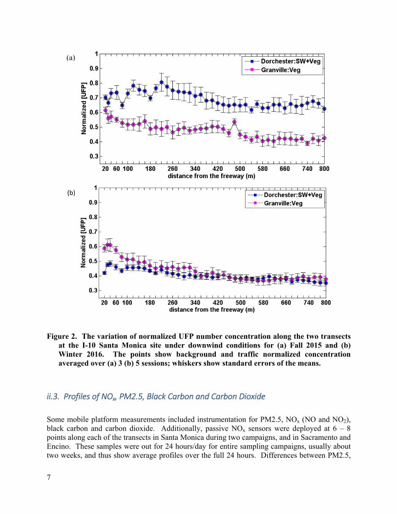
Analysis of data for Santa Monica indicate that under some conditions, concentrations are lower at the combination tree and solid barrier and the relatively thick stand of trees, in other cases the reverse is true (Figure 2). Differences may be due to wind speed. Effects of vegetation under calm conditions need further study.

7

Figure 2. The variation of normalized UFP number concentration along the two transects at the I-10 Santa Monica site under downwind conditions for (a) Fall 2015 and (b) Winter 2016. The points show background and traffic normalized concentration averaged over (a) 3 (b) 5 sessions; whiskers show standard errors of the means.

ii.3.  Profiles of NOx, PM2.5, Black Carbon and Carbon Dioxide 

Some mobile platform measurements included instrumentation for PM2.5, NOx (NO and NO2), black carbon and carbon dioxide. Additionally, passive NOx sensors were deployed at 6 – 8 points along each of the transects in Santa Monica during two campaigns, and in Sacramento and Encino. These samples were out for 24 hours/day for entire sampling campaigns, usually about two weeks, and thus show average profiles over the full 24 hours. Differences between PM2.5,

(a)

(b)

8

black carbon and carbon dioxide upwind and downwind concentrations of the two barriers at the Sacramento site were generally not significant. Profiles for NOx species however, generally did show significant differences, consistent with fact that freeways generally have higher NOx concentrations compared to their backgrounds, and thus have a clearer signal.

For Sacramento, both mobile platform NO and NO2, as well as passive NOx samples all showed significantly lower concentrations downwind of the combination vegetation/solid sound wall compared to the sound wall-only site. The NOx plumes also reached out further than the UFP plumes; 300 – 350 m for NOx vs. 100 – 150 m for UFP. The Encino passive NOx measurements were also significantly lower downwind of the combination barrier compared to the vegetation-only barrier (Figure 3). At this site, the trees at the vegetation-only transect were less dense than those at the combination barrier. At the Santa Monica site, a pronounced decay profile was absent. The Santa Monica site was chosen to study calm atmospheric conditions. These conditions occur in the mornings when pollutant concentrations can be very high, as well as at night when emissions are typically low. However, for most the day, the target area is upwind of the freeway and intersects some busy surface streets. Thus, while there is a pronounced plume from the freeway in the morning, profiles are indistinct over 24 hours, and there is no obvious difference between the two barrier configurations (i.e., vegetation-only barrier vs. combination barrier).

Figure 3. Average profiles for NO and NO2 at the Encino site, illustrating reductions attributed to the combination of vegetation and a solid soundwall, compared to vegetation alone.

ii.4 Continuous Measurements Near the Barriers 

We conducted continuous measurements at fixed sites located close to the barriers. When aggregated, this data provides overall average differences at these sites. We performed spatial difference-in-differences (DID) analyses on the concurrent measurements at three to four stationary sampling locations at each site. Overall findings of this analysis are that the concentration reductions of the listed particle species were greater with a combination barrier of soundwall and vegetation than either one alone. With respect to the measurements downwind of

9

a vegetation-only barrier, we found 18% reduction of total particle number concentration (e.g., UFP number concentration) and 11% reduction of PM2.5 mass concentration at average wind speed of 1.00 m/s in Encino. At lower average wind speed, 0.79 m/s in Santa Monica, an additional soundwall barrier made little differences in UFP (6.9%) and PM2.5 (4.7%). Under the same conditions, the overall reduction of BC was found to be 24% at wind speed of 0.79 m/s in Santa Monica and 28% at 1.00 m/s in Encino. The small change of wind speed is found to increase or decrease the effectiveness of an additional soundwall barrier in the vegetated area.

In addition, examination of the overall reduction of UFP number concentration, especially at smaller sizes was greater with additional vegetation than with an additional soundwall barrier, potentially because of larger surface area of the foliage, which resulted in greater reductions of the particles smaller than 80 nm. On the other hand, an additional soundwall barrier was found more effective (18%) on reducing PM2.5 mass concentration with respect to the existing vegetation, likely due to the dispersion and dilution enhanced by a structure of soundwall barrier.

ii.5 Model Development 

We developed and applied a dispersion model to estimate concentrations of vehicle related emissions downwind of a barrier consisting of vegetation planted next to a solid noise barrier. The model is based on the analysis of UFP data collected in Riverside, and Sacramento. The objective of the Riverside study was to evaluate and, if necessary, modify a model for dispersion of emissions from a highway with solid barriers located on its sides. The results suggest the model provides reliable estimates of the impact of a solid noise barrier on concentrations of highway emissions downwind of the barrier, including both the magnitude as well as the spatial variation of UFP concentrations measured during the field study. The model predicts that a 4 m barrier results in a 35% reduction in average concentration within 40 m (10 barrier heights) of the barrier, relative to the no-barrier site. The predicted reduction is 55% if the barrier height is doubled. The Riverside results reinforce earlier conclusions that the presence of the barrier is equivalent to shifting the line sources on the road upwind by a distance of about the barrier height multiplied by the ratio of the near surface wind speed and the vertical turbulent velocity. If we take a typical value of the ratio as 0.2 and the barrier height as 5 m, the mitigation effect of the barrier is equivalent to shifting the highway upwind of a receptor by a distance of about 25 m.

The Sacramento data were used to investigate the impact of adding vegetation behind a solid wall on downwind concentrations associated with highway emissions. The data indicated that about 25% of the 15-minute averaged UFP concentrations measured downwind of the vegetation-solid barrier were higher than those downwind of the barrier without vegetation: the vegetation reduced the mitigating effect of the solid barrier. This result appeared to be related to the reduction of turbulence caused by vegetation, which decreases dispersion and increases concentrations relative to those downwind of the plain barrier. This hypothesis is supported by the analysis of turbulence levels measured by the sonic anemometers located downwind of the two barriers. We used the ratio of the turbulence levels measured below wall height as surrogates for the ratios of the turbulence levels that governed dispersion of the plumes traveling over the barrier. The ratio of the concentration measured downwind of the vegetation-solid barrier to that measured simultaneously downwind of the plain barrier indicates the benefit of the vegetation added to the solid barrier We found that this ratio increased from values below one

10

to values above one as the ratio of the turbulence levels downwind of the two barriers decreased. The data also show that the ratio of the turbulence levels decreased as the upwind wind speed and turbulence increased. This suggests that the additional mitigation related to the vegetation decreases as the upwind wind speed increases; at some point, the additional vegetation can counteract the mitigating effect of the solid barrier.

As the first step in modeling the complex effects of vegetation, we applied the modified mixed wake model to interpret the results. We accounted for the effects of vegetation through three modifications: 1) the friction velocity is multiplied by the ratio of vertical velocity fluctuation,

, behind the vegetation-wall to wall barrier to model the reduction of turbulence by the vegetation, 2) the entrainment of material into the wake is reduced by the ratio of turbulent velocities, and 3) the effective height of the wall is increased to account for additional plume lofting induced by the vegetation. Evaluation of the model with measurements indicates that over 90% of the model estimates were within a factor of two of the corresponding observations, although the correlation was poor. However, the model could not reproduce the concentrations downwind of the vegetation-solid barrier being higher than those downwind of the solid barrier, although it produced comparable magnitudes for these cases.

The model was then used to estimate the expected spatial variation of concentrations downwind of the two wall sites: wall plus vegetation and the wall. We find that the addition of vegetation increases the mitigation effect of the solid wall within 100 m from the wall; the additional reduction ranges from 25% close to the wall to 10% at 30 m. The model predicts that addition of vegetation to a solid wall does confer additional mitigation, but the effect is relatively small for the type of vegetation considered in this field study (Figure 4). The dispersion and planning guidance model developed under this project is titled “Model for Impact of Roads with Barriers (MIRB)”, and is available at https://www.arb.ca.gov/research/single-project.php?row_id=65195.

Figure 4. Left panel: Concentration gradients predicted by the model for wall, vegetation-wall. Right panel: Concentration ratio predicted by model for wall and vegetation-wall barrier.

11

ii.6 Summary & Conclusion 

In summary, adding vegetation that exceeds the height of the barrier appears to be a clear benefit, especially if the vegetation is tall and dense. This configuration effectively extends the height of the solid barrier. There is evidence of a small dis-benefit at higher wind speeds likely due to reduction in turbulence downwind of the vegetation. However, as pollution dispersion is generally higher and concentrations lower under higher wind speeds regimes, the benefits at lower wind speeds should out-weigh a modest dis-benefit at high wind speeds. The benefit is clear during daytime, and the same conclusion is also supported from results from the early mornings when winds are weak the atmosphere more stable. Table 1 shows recommendations for specific scenarios.

Table 1. Situations for which addition of vegetation to existing solid barriers is likely to reduce concentrations of roadway pollutants.(1)

         Predominant  Wind 

Direction 

 

 

Receptor 

Downwind during daytime; moderate winds 

Downwind during night/morning/under calm conditions (winds < about 1 m/s) 

Downwind during day or night; nights and mornings are often calm 

Usually breezy or windy; calm conditions are uncommon 

Residential Neighborhood within ~150 m(2) 

Residential Neighborhood further than 150 m, within ~500 m(3) 

Minimal impact(4)

Minimal impact(4)

School, hospital, residential facility for the elderly etc.  within ~150 m(2) 

(5)

(5)

School, hospital, residential facility for the elderly etc.  further than 150 m, within ~500 m(3) 

Minimal impact(4)

Minimal impact(4)

Park used mostly in afternoons on weekdays, all day during weekends 

Limited

Impact(6)

Limited to minimal

impact(4) (6)

12

1This Table is provided as a general guide for planners. The specific geometry of a particular site may produce different outcomes; site-specific measurements are advisable. “Roadway pollutants” is limited to pollutants that are elevated around roadways. This usually includes ultrafine particles, oxides of nitrogen (especially NO), traffic-related volatile organic compounds, and especially around roadways with substantial heavy duty truck traffic, black carbon. Road dust and brake wear particles can also be elevated around roadways, but have different spatial dynamics than the gas phase and small particles studied here, and thus is not included. Further, PM2.5 is typically only slightly elevated around roadways, and is also not included. 2See section 3.1 3See section 3.2 4”Minimal impact” indicates very low impact. 5Moving physical education classes to later in the day will also reduce exposures where morning concentrations are high. 6”Limited impact” indicates minimal impact for most of the day, but impacts may be significant during the morning periods.

iii.  Acknowledgements Dr. Wonsik Choi was partially funded by Korean Ministry of Environment through "Climate Change Correspondence Program". The mobile monitoring platform measurements were made possible with the additional assistance of Mr. Steve Mara. We also thank Mr. Steve Mara and Drs. Walter Ham, Nico Schulte, Toshi Kuwayama (ARB) for assistance with Sacramento field measurements. We thank Dr. Matthias Falk for identifying the tree species at the Sacramento site. Ms. Ruiting Christine Qin (UCLA) provided expert editorial assistance. We also ARB staff including Drs. Kathleen Kozawa, Walter Ham, Abhilash Vijayan and Mrs. Bart Croes and Steve Mara, Mses. Emma Plasencia, Trish Chancy and Monica Vejar for contract support.

The views and opinions in this study are those of the authors and do not reflect the official views of CARB.

13

iv. Table of Contents i.  Abstract .................................................................................................................................... 2 

ii.  Executive Summary ................................................................................................................. 4 

ii.1 Vegetation Characterization .................................................................................................. 5 

ii.2 Decay Profiles of Ultrafine Particles .................................................................................... 6 

ii.3. Profiles of NOx, PM2.5, Black Carbon and Carbon Dioxide ............................................. 7 

ii.4 Continuous Measurements Near the Barriers ....................................................................... 8 

ii.5 Model Development .............................................................................................................. 9 

ii.6 Summary & Conclusion ...................................................................................................... 11 

iii. Acknowledgements ................................................................................................................ 12 

iv.  Table of Contents .............................................................................................................. 13 

v.  List of Tables ......................................................................................................................... 16 

vi.  List of Figures ................................................................................................................... 18 

vii.  List of Abbreviations ........................................................................................................ 26 

1.  Introduction and Background ................................................................................................ 27 

1.1 Background ......................................................................................................................... 27 

1.2 The Impact of Solid Barriers ............................................................................................... 28 

1.3 Observations on the Impact of Vegetative Barriers ............................................................ 33 

1.4 Models for the Impact of Vegetative Barriers ..................................................................... 34 

1.5 Summary and Objectives for Current Study ....................................................................... 35 

2.  Methods ................................................................................................................................. 36 

2.1 Descriptions of Sampling Sites ........................................................................................... 36 

2.2 Traffic flow and Overview of Wind Data ........................................................................... 41 

2.2.1 Detailed Traffic Analysis.............................................................................................. 45 

2.2.2 Encino Meterological Measurements ........................................................................... 49 

2.2.3 Santa Monica Meteorological Measurements .............................................................. 54 

14

2.2.4 Sacramento Meteorological Measurements .................................................................. 56 

2.2.5 Riverside Meteorological Measurements ..................................................................... 59 

2.3 Continuous Stationary Measurements ................................................................................. 62 

2.3.1 Particle size distributions, PM2.5 and black carbon ..................................................... 62 

2.3.1.1 Riverside Particle Measurements .......................................................................... 63 

2.3.2 Passive Measurements of NO and NO2 ........................................................................ 64 

2.3.3 Difference-in-Differences Analysis .............................................................................. 65 

2.4 Mobile Measurements ......................................................................................................... 65 

2.4.1 Mobile Measurements Description ............................................................................... 65 

2.4.2 Data Analysis and Concentration Profiles .................................................................... 69 

2.5 Vegetation Characterization ................................................................................................ 71 

3.  Results and Discussion .......................................................................................................... 73 

3.1 Optical Porosity of Vegetation at the Santa Monica, Sacramento and Encino Sites .......... 73 

3.2 I-10 Santa Monica Profiles, Continuous Fixed-Site Results and Vegetation Characterization ........................................................................................................................ 76 

3.2.1 Vegetation Characterization ......................................................................................... 76 

3.2.2 Decay Profiles from Mobile and Passive Measurements ............................................. 79 

3.2.3 Continuous Measurements from Passive Samplers: NO and NO2 Profiles .................. 82 

3.2.4 Continuous Paired-Site Measurements of UFP, PM2.5, and BC ................................. 84 

3.2.5 Difference-in-Differences ............................................................................................. 88 

3.3 I-101 Encino Profiles, Continuous Fixed-Site Results and Vegetation Characterization ... 90 

3.3.1 Vegetation Characterization ......................................................................................... 90 

3.3.2 Decay Profiles from Mobile and Passive Monitoring .................................................. 93 

3.3.3 Continuous Passive NO and NO2 Profiles .................................................................... 94 

3.3.4 Additional Stationary Measurements: UFP, PM2.5, and BC ...................................... 96 

3.3.5 Difference-in-Differences ............................................................................................. 99 

3.3.5.1 Discussion of Encino and Santa Monica Results ................................................ 101 

15

3.4 Sacramento CA-99 Profiles, Continuous Fixed-Site Results and Vegetation Characterization ...................................................................................................................... 102 

3.4.1 Vegetation Characterization ....................................................................................... 102 

3.4.2 Decay Profiles from Mobile and Passive Measurements ........................................... 105 

3.4.3 Profiles from Passive NO and NO2 Profiles ............................................................... 108 

3.4.4 Additional Continuous Measurements: UFP, PM2.5, and BC .................................. 110 

3.4.5 Difference-in-Differences ........................................................................................... 114 

3.4.5.1 Dependence of Differences on Particle Size ....................................................... 117 

3.7 Wind speed dependence of [UFP] pollution reduction ..................................................... 118 

3.8 Modeling the Impact of Vegetation-Solid Barriers on Near Road Air Quality ................ 121 

3.8.1 Introduction ................................................................................................................ 121 

3.8.2 Riverside Results ........................................................................................................ 121 

3.8.2.1 Dispersion Modeling ........................................................................................... 121 

Simple Barrier Model ..................................................................................................... 124 

3.8.2.2 Modified mixed-wake model .............................................................................. 124 

3.8.2.3 Modeling Results ................................................................................................ 126 

3.8.3 Sacramento Results ..................................................................................................... 130 

3.8.3.1 Air Quality and Meteorological Measurements .................................................. 130 

3.8.3.2 Measurement Results .......................................................................................... 132 

3.8.4 Modeling Framework ................................................................................................. 135 

3.8.5Summary and Conclusions for modeling results ......................................................... 137 

4.  Summary and Conclusions .................................................................................................. 139 

4.1 Overview ........................................................................................................................... 139 

4.2 Summary and Conclusions ................................................................................................ 139 

4.3 Summary for Planners ....................................................................................................... 141 

5.  References ........................................................................................................................... 144 

16

v. List of Tables  Table 1. Situations for which addition of vegetation to existing solid barriers is likely to reduce concentrations of roadway pollutants.(1) ....................................................................................... 11 

Table 2. A summary of traffic flow and wind speed data from three sampling sites. The data are given in arithmetic averages and one standard deviations from all data collected under the specific wind direction as noted. This data corresponds to continuous stationary data collected at continuous stationary sampling sites. ........................................................................................... 42 

Table 3. Overview of measurement in Santa Monica .................................................................. 55 

Table 4. Overview of the dates and time of measurement in Sacramento. .................................. 59 

Table 5. Meteorological conditions in Riverside study. .............................................................. 61 

Table 6. Overview of dates and duration of measurements in Riverside. ................................... 63 

Table 7. Monitoring instruments on the mobile monitoring platform. ........................................ 66 

Table 8. Measurement periods and surface meteorology at the sites. ......................................... 69 

Table 9. Average height and average porosity of trees at each location on the primary downwind side, and max height of any vegetation at either of each pair of sites, and the corresponding optical porosity for the max height. .............................................................................................. 74 

Table 10. Very approximate optical porosity for some representative tree species observed at the study sites in Southern California ................................................................................................. 76 

Table 11. Tree species observed at the Santa Monica transects .................................................. 79 

Table 12. A summary of NO and NO2 data in tabular form for the data in Figure 43 along the I-10 freeway in Santa Monica, CA. ................................................................................................. 84 

Table 13. A summary of UFP, PM2.5, BC concentration measurements at the upwind and downwind sampling locations of vegetation only (VO) and vegetation with soundwall (VW) sites along the I-10 freeway in Santa Monica, CA. .............................................................................. 87 

Table 14. A summary of downwind-upwind differences and difference-in-differences (DID) for UFP, PM2.5, BC measurements in the areas with vegetation only (dVO) and with vegetation and soundwall (dVW) near the I-10 in Santa Monica, CA. The DID values are the difference of dVO and dVW. ...................................................................................................................................... 90 

Table 15. NO and NO2 concentrations from Ogawa samplers deployed at Encino Mar. 24 – Apr. 8, 2016. ................................................................................................................................ 95 

Table 16. A summary of UFP, PM2.5, BC concentration measurements at the upwind and downwind sampling locations of vegetation only (VO) and vegetation with soundwall (VW) sites along the I-101 freeway in Encino, CA. ....................................................................................... 98 

17

Table 17. A summary of downwind-upwind differences and difference-in-differences (DID) for UFP, PM2.5, BC measurements in the areas with vegetation only (dVO) and with vegetation and soundwall (dVW) near the I-101 in Encino, CA. The DID values are the difference of dVO and dVW. ........................................................................................................................................... 101 

Table 18. Continuous passive NO and NO2 data for the Sacramento site. ............................... 110 

Table 19. A summary of UFP, PM2.5, BC concentration measurements at the upwind and downwind sampling locations of soundwall only (WO) and vegetation with soundwall (VW) sites along the CA-99 freeway in Sacramento, CA .................................................................... 113 

Table 20. A summary of downwind-upwind differences and difference-in-differences (DID) for UFP, PM2.5, BC measurements in the areas with soundwall only (dWO) and with vegetation and soundwall (dVW) near the CA-99 in Sacramento, CA. The DID values are the difference of dWO and dVW. .......................................................................................................................... 117 

Table 21. Overview of the dates and time of measurement in Sacramento. .............................. 132 

Table 22. Characteristics of plumes around freeways ............................................................... 141 

Table 23. Situations for which addition of vegetation to existing solid barriers is likely to reduce concentrations of roadway pollutants.(1) ..................................................................................... 142 

 

18

vi. List of Figures  Figure 1. Average profiles for ultrafine particles at the Sacramento site, illustrating reductions attributed to the addition of vegetation behind a solid soundwall. The points show background and traffic normalized average concentrations; black whiskers show standard errors of the means. ............................................................................................................................................. 6 

Figure 2. The variation of normalized UFP number concentration along the two transects at the I-10 Santa Monica site under downwind conditions for (a) Fall 2015 and (b) Winter 2016. The points show background and traffic normalized concentration averaged over (a) 3 (b) 5 sessions; whiskers show standard errors of the means. .................................................................................. 7 

Figure 3. Average profiles for NO and NO2 at the Encino site, illustrating reductions attributed to the combination of vegetation and a solid soundwall, compared to vegetation alone. ............... 8 

Figure 4. Left panel: Concentration gradients predicted by the model for wall, vegetation-wall. Right panel: Concentration ratio predicted by model for wall and vegetation-wall barrier. ........ 10 

Figure 5. Flow induced by physical barrier (Steffens et al., 2013). ............................................. 29 

Figure 6. Mock straw bale sound barrier, 6m high and 90 m long (Finn et al. 2010). ............... 30 

Figure 7. Spatial variation of SF6 concentration measured in the Idaho Falls experiment. The barrier height is 6 m. Points represent averages over maximum concentrations measured over the 3 hours of each experiment. Upper lines (blue) indicate concentrations in the absence of the barrier, and lower (red) with the barrier. ....................................................................................... 30 

Figure 8. Vertical distribution of normalized concentrations (χ) at 20 m/3.3H (a), 50 m/8.3H (b), 150 m/25H (c), and 300 m/50H (d) from the edge of the roadway under perpendicular winds, for barriers of 3 to 18 m compared with a no-barrier scenario. The barrier is located 9.5m from the road edge (Hagler et al., 2011). ..................................................................................................... 32 

Figure 9. Comparison between modeled and observed maximum concentrations at different downwind distances. The maximum concentrations are averaged over the 3 hours of each experiment..................................................................................................................................... 33 

Figure 10. Mobile monitoring measurements of (a) 20 nm and (b) 75 nm size particles using the DMA–CPC units at varying distances from the road for open terrain, behind a noise barrier only, and behind a noise barrier with vegetation. Bars represent 95% confidence intervals for each distance (Baldauf et al. 2008). ..................................................................................................... 34 

Figure 11. An aerial image of the sampling site near I-10 freeway in Santa Monica, CA. Each sampling locations are marked in circles of different schemes: solid black line and dashed green line indicate the presence of soundwall and vegetation, respectively. The gray arrow shows the wind direction desirable at this sampling site. .............................................................................. 37 

Figure 12. An aerial image of the sampling site near I-101 freeway in Encino, CA. Each sampling locations are marked in circles of different schemes: solid black line and dashed green line indicate the presence of soundwall and vegetation, respectively. The gray arrow shows the wind direction desirable at this sampling site. .............................................................................. 38 

19

Figure 13. An aerial image of the sampling site near CA-99 freeway in Sacramento, CA. Each sampling locations are marked in circles of different schemes: solid black line and dashed green line indicate the presence of soundwall and vegetation, respectively. The gray arrow shows the wind direction desirable at this sampling site. .............................................................................. 39 

Figure 14. A time-series of diurnal traffic flow (veh./5-min, dark gray) and wind speed (m/s, light gray) under (a) Northerly Wind (WD ≥ 300 ° or WD < 30 °) and (b) Southerly Wind (120 ≤ WD < 210 °) conditions at the I-10 sampling site in Santa Monica, CA. ..................................... 43 

Figure 15. A time-series of diurnal traffic flow (veh./5-min, dark gray) and wind speed (m/s, light gray) at two sampling sites: (a) I-101 in Encino and (b) CA-99 in Sacramento. ................. 44 

Figure 16. The location of PeMS sensors used in the traffic flow calculations at the Santa Monica site. The yellow stars note the location of the measurement transects. The green circles show the main line sensors used in the calculation. Green arrows show the ramps with data available and red arrows show the ramps with no data available. ................................................ 45 

Figure 17. The diurnal traffic flow variation on I 10 at Santa Monica site, during (a) fall and (b) winter measurement sessions. The 30 min mean of the traffic flow in both directions at each measurement transect (color symbols) and the standard deviation of the mean. Different symbols indicate different measurement days. ........................................................................................... 47 

Figure 18. A schematic showing locations of PeMS sensors used in the traffic flow calculations at the Encino site. The yellow starts note the location of the measurement transects. The green circles show the main line sensors used in the calculation. Green arrows show the ramps with data available and red arrows show the ramps with no data available. ........................................ 47 

Figure 19. The diurnal traffic flow variation on I 101 at Encino site. The 30 min mean of the traffic flow in both directions and the standard deviation of the mean. Different symbols indicate different measurement days. ......................................................................................................... 48 

Figure 20. A schematic showing locations of PeMS sensors used in the traffic flow calculations at the Sacramento site. The yellow starts note the location of the measurement transects. The green/yellow circles show the main line sensors used in the calculation. Green arrows show the ramps with data available. ............................................................................................................. 48 

Figure 21. The diurnal traffic flow variation on SR 99 at Sacramento site. (a) The 30 min mean of the traffic flow in both directions at each measurement transect (color symbols) and the standard deviation of the mean. Different symbols indicate different measurement days. (b) The 30 min mean of the traffic flow in both directions, averaged of all measurement days, and the standard deviation of the mean. .................................................................................................... 49 

Figure 22- Location of installed sonic anemometer and Van Nuys meteorological station during Encino field study ......................................................................................................................... 50 

Figure 23- Time series of wind direction data from Feb. 17th 2016– Feb. 28th 2016 collected by the sonic anemometer ( ) and by ASOS ( ). ................................................................................. 52 

20

Figure 24. Frequencies in each wind direction based on a) sonic anemometer and b) ASOS data........................................................................................................................................................ 53 

Figure 25. a) Wind rose for the data collected by Van Nuys sonic anemometer from February 17th to February 29th. b) Wind rose for the data collected by Van Nuys meteorological station from February 17th to February 29th 2016. .................................................................................... 53 

Figure 26. Location of sonic anemometers in Santa Monica study ............................................. 54 

Figure 27. Wind rose for the data collected at Santa Monica during October 2015 .................... 55 

Figure 28. Instrument locations in Sacramento site. .................................................................... 56 

Figure 29. a) view of wall vegetation barrier. b) view of barrier and downwind anemometer behind it. ....................................................................................................................................... 57 

Figure 30. Wind rose from Sacramento Executive Airport meteorological station during June 2016............................................................................................................................................... 58 

Figure 31. Map of the selected site in Riverside. Adapted from Google Earth. ......................... 60 

Figure 32. Wind rose from UC Riverside meteorological station and freeway direction at barrier site during February 2015. ............................................................................................................ 60 

Figure 33. Approximate location of instruments in Riverside site. ............................................. 64 

Figure 34. The mobile sampling route at the I-10 site in Santa Monica, CA (blue lines). The yellow dots denote the upwind semi-stationary measurement locations. The green lines denote the location of the vegetation barriers and the red lines denote location of the sound walls. Map source: Google Earth. .................................................................................................................... 67 

Figure 35. The mobile sampling route at the I-101 site in Encino, CA (blue lines). The yellow dots denote the upwind semi-stationary measurement locations. The green lines denote the location of the vegetation barriers and the red line denotes location of the sound wall. Map source: Google Earth. .................................................................................................................... 68 

Figure 36. The mobile sampling route at the SR-99 site in Sacramento, CA (blue lines). The yellow dots denote the upwind semi-stationary measurement locations. The green lines denote the location of the vegetation barriers and the red lines denote location of the sound wall. Map source: Google Earth. .................................................................................................................... 68 

Figure 37. Effective optical porosity as a function of height. The solid lines indicate the heights up to the maximum height of any tree in the scene; dotted lines include increasing amounts of clear sky. High porosity corresponds to low tree density and/or gaps between trees. ................. 75 

Figure 38. Aerial view and locations of trees labelled in Figure 40 at the Granville transect in Santa Monica. ............................................................................................................................... 77 

Figure 39. Aerial view and locations of trees labelled in Figure 40 at the Granville transect in Santa Monica. ............................................................................................................................... 77 

21

Figure 40. Profile view and top view of the tree canopies along the I-10 sections near Granville Avenue (top two panels) and near Dorchester Avenue (bottom two panels). In the profile view panels, tree columns are colored coded by the optical porosity. .................................................. 78 

Figure 41. The variation of normalized UFP number concentration along the two transects at the I-10 Santa Monica site under downwind conditions for (a) Fall 2015 and (b) Winter 2016 measurement sessions. The background and traffic normalized concentration averaged over (a) 3 (b) 5 sessions (color points) is plotted together with the standard error of the mean (black whiskers). ...................................................................................................................................... 80 

Figure 42. The variation of normalized UFP number concentration along the two transects at the I-10 Santa Monica site, under parallel wind conditions for (a) Fall 2015 and (b) Winter 2016 measurement sessions. The background and traffic normalized concentration averaged over 4 sessions (color points) is plotted together with the standard error of the mean (black whiskers). 81 

Figure 43. NO and NO2 concentration data collected from Ogawa passive samplers distributed near I-10 in Santa Monica during May-June 2015 along (a) Dorchester Ave. (vegetation and soundwall); and, (b) Granville Ave. (vegetation only). ............................................................... 82 

Figure 44. NO and NO2 concentration data collected from Ogawa passive samplers distributed near I-10 in Santa Monica during Sept.-Oct. 2015 along (a) Dorchester Ave. (vegetation and soundwall); and, (b) Granville Ave. (vegetation only). ............................................................... 83 

Figure 45. NO and NO2 concentration data collected from Ogawa passive samplers distributed near I-10 in Santa Monica during Feb. - March 2016 along (a) Dorchester Ave. (vegetation and soundwall); and, (b) Granville Ave. (vegetation only). ............................................................... 83 

Figure 46. Wind rose for data in Figure 43. The gray arrow indicates the orientation of I-10. .. 84 

Figure 47. Particle size distribution data collected under different configurations: (a) vegetation only and (b) vegetation and soundwall at the study site near I-10 in Santa Monica. Different color schemes indicate the data collected at upwind (gray) and downwind (black) sampling locations. The log-normalized particle number concentration (dN/dLogDp) data are the medians of measurements under southerly wind conditions (165 ± 45°) and plotted with respect to aerodynamic diameter (Dp). ......................................................................................................... 85 

Figure 48. Total number particle concentrations for: vegetation only (left) and vegetation with soundwall (right) at the study site near I-10 in Santa Monica. Different color schemes indicate the data collected at upwind (dark gray) and downwind (light gray) sampling locations. The medians of the data collected under southerly wind conditions (165 ± 45°) are plotted. The error bars indicate one standard deviation. ............................................................................................ 86 

Figure 49. (a) PM2.5 and (b) black carbon (BC) data collected under different configurations: vegetation only (left) and vegetation with soundwall (right) at the study site near I-10 in Santa Monica. Different color schemes indicate the data collected at upwind (dark gray) and downwind (light gray) sampling locations. The medians of the data collected under northerly wind conditions (345 ± 45°) are plotted. The error bars indicate one standard deviation of the measurements. ............................................................................................................................... 87 

22

Figure 50. Downwind-upwind differences and Difference-in-Differences (DID) for total number particle concentrations for vegetation only (dVO, black) and vegetation and soundwall (dVW, gray) near the I-10 in Santa Monica, CA. The dark gray bar indicates the DID value (i.e., DID = dVO – dVW). Medians with one standard deviation are shown. ................................................ 88 

Figure 51. Downwind-upwind differences and Difference-in-Differences (DID) for (a) PM2.5 and (b) black carbon. The differences are shown for the study areas with vegetation only (dVO, black) and with vegetation and soundwall (dVW, gray) near the I-10 in Santa Monica, CA. The dark gray bar indicates the DID value (i.e., DID = dVO – dVW). The plotted data are the medians and the error bars indicate one standard deviation. ........................................................ 89 

Figure 52. Aerial view and locations of trees labelled in Figure 40 at the Zelzah Ave. transect in Encino. This location has no soundwall, and a low level of vegetation in the neighborhood. .... 91 

Figure 53. Aerial view and locations of trees labelled in Figure 40 at the Encino Ave. transect in Encino. This location has a soundwall, in addition to relatively dense vegetation in the neighborhood. ............................................................................................................................... 91 

Figure 54. Profile view and top view of the tree canopies along the I-101 sections near Zelzah Avenue (top two panels) and near Encino Avenue (bottom two panels). In the profile view panels, tree columns are colored coded by the optical porosity. .................................................. 92 

Figure 55. The variation of the normalized UFP number concentration along the two transects at the I-101 Encino site, under (a) downwind and (b) parallel wind conditions. The traffic normalized concentration of a session (color plots) is plotted together with the standard error of the mean (black). ........................................................................................................................... 93 

Figure 56. NO and NO2 concentration data collected from Ogawa passive samplers distributed near I-101 in Encino during Mar.-April 2016 along (a) Encino Ave. (vegetation and soundwall); and, (b) Zelzah Ave. (vegetation only). ....................................................................................... 94 

Figure 57. Wind rose for March 24 -Apr 8, 2016 at Encino. The gray arrow indicates the orientation of I-101. ...................................................................................................................... 95 

Figure 58. Particle size distribution data collected under different configurations: (a) vegetation only and (b) vegetation and soundwall at the study site near I-101 in Encino. Different color schemes indicate the data collected at upwind (gray) and downwind (black) sampling locations. The log-normalized particle number concentration (dN/dLogDp) data are the medians of measurements under northerly wind conditions (0 ± 45°) and plotted with respect to aerodynamic diameter (Dp). ............................................................................................................................... 96 

Figure 59. Total number particle concentration data collected under different configurations: vegetation only (left) and vegetation with soundwall (right) at the study site near I-101 in Encino. Different color schemes indicate the data collected at upwind (dark gray) and downwind (light gray) sampling locations. The medians of data collected under northerly wind conditions (0 ± 45°) are plotted. The error bars indicate one standard deviation. ................................................ 97 

Figure 60. (a) PM2.5 and (b) black carbon (BC) data collected under different configurations: vegetation only (left) and vegetation with soundwall (right) at the study site near I-101 in Encino.

23

Different color schemes indicate the data collected at upwind (dark gray) and downwind (light gray) sampling locations. The medians of the data collected under northerly wind conditions (0 ± 45°) are plotted. The error bars indicate one standard deviation of the measurements. ........... 98 

Figure 61. Downwind-upwind differences and Difference-in-Differences (DID) for total number particle concentrations. The differences are shown for the study areas with vegetation only (dVO, black) and with vegetation and soundwall (dVW, gray) near the I-101 in Encino, CA. The dark gray bar indicates the DID value (i.e., DID = dVO – dVW). The plotted data are the medians and the error bars indicate one standard deviation. ........................................................ 99 

Figure 62. Downwind-upwind differences and Difference-in-Differences (DID) for (a) PM2.5 and (b) black carbon. The differences are shown for the study areas with vegetation only (dVO, black) and with vegetation and soundwall (dVW, gray) near the I-101 in Encino, CA. The dark gray bar indicates the DID value (i.e., DID = dVO – dVW). The plotted data are the medians and the error bars indicate one standard deviation. ..................................................................... 100 

Figure 63. Google Earth photograph of CA-99 near the intersection with 9th Ave. in Sacramento, and adjacent streets. Yellow pins and accompanying white numbers indicate specific trees or groups of trees labelled in Figure 65. ............................................................... 102 

Figure 64. Google Earth photograph of CA-99 near the intersection with 19th Ave. in Sacramento, and adjacent streets. Yellow pins and accompanying white numbers indicate specific trees or groups of trees labelled in Figure 65. ............................................................... 103 

Figure 65. Profile view and top view of the tree canopies along the CA-99 sections near the 9th Avenue (top two panels) and near the 19th Avenue (bottom two panels). In the profile view panels, tree columns are colored coded by the optical porosity. The “average optical porosity” indicates the average at the average height of the tree canopy. .................................................. 104 

Figure 66. The variation of normalized UFP number concentration along the two transects at the SR-99 Sacramento site, under (a) downwind and (b) parallel wind conditions. The background and traffic normalized concentration averaged over (a) 6 (b) 4 sessions (color plots) is plotted together with the standard error of the mean (black). ................................................................. 106 

Figure 67. The variation of normalized (a) PM 2.5, (b) Black Carbon and (c) CO2 concentration along the two transects at the SR-99 Sacramento site. ............................................................... 107 

Figure 68. The variation of normalized (a) NO, (b) NO2 concentration along the two transects at the SR-99 Sacramento site. ......................................................................................................... 108 

Figure 69. NO and NO2 concentration data collected from Ogawa passive samplers distributed near CA-99 during June-July 2016 along (a) 19th Ave (soundwall and vegetation); and, (b) 9th Ave. (soundwall only). ............................................................................................................... 109 

Figure 70.Wind rose for the Sacramento study. ......................................................................... 109 

Figure 71. Particle size distribution data collected under different configurations: (a) soundwall only and (b) vegetation and soundwall at the study site near CA-99 in Sacramento. Different color schemes indicate the data collected at upwind (gray) and downwind (black) sampling

24

locations. The log-normalized particle number concentration (dN/dLogDp) data are the medians of measurements under southerly wind conditions (165 ± 45°) and plotted with respect to aerodynamic diameter (Dp). ....................................................................................................... 111 

Figure 72. Total number particle concentration data collected under different configurations: soundwall only (left) and vegetation with soundwall (right) at the study site near CA-99 in Sacramento. Different color schemes indicate the data collected at upwind (dark gray) and downwind (light gray) sampling locations. The medians of the data collected under westerly wind conditions (270 ± 45°) are plotted. The error bars indicate one standard deviation of the measurements. ............................................................................................................................. 112 

Figure 73. Median PM2.5 mass concentrations for soundwall only (left) and vegetation with soundwall (right) at the study site near CA-99 in Sacramento under westerly wind conditions (270 ± 45°). No data were collected at the upwind sampling locations. The error bars indicate one standard deviation. ............................................................................................................... 113 

Figure 74. Median downwind-upwind differences and Difference-in-Differences (DID) for total number particle concentrations for soundwall only (dWO, black) and soundwall and vegetation (dVW, gray) near the CA-99 in Sacramento. The dark gray bar indicates the DID value (i.e., DID = dWO – dVW). The error bars indicate one standard deviation. ..................................... 114 

Figure 75. Median downwind-upwind differences and Difference-in-Differences (DID) for PM2.5 for soundwall only (dWO, black) and with soundwall and vegetation (dVW, gray) sites near CA-99 in Sacramento. The dark gray bar indicates the DID value (i.e., DID = dWO – dVW). The error bars indicate one standard deviation. ............................................................. 116 

Figure 76. Difference-in-differences (DID) of dN/dLogDp data collected with (a) additional soundwall (near I-101 in Encino; DID = dVO – dVW) and (b) additional vegetation (near CA-99 in Sacramento; DID = dWO – dVW). Medians of the DID estimates are plotted with respect to aerodynamic diameter (Dp). ....................................................................................................... 118 

Figure 77. The relative [UFP] reduction by a combination barrier, under downwind conditions, averaged over the first 160 m from the edge of the freeway for (a) Santa Monica: VO-VW/VO and (b) Sacramento: WO-VW/WO, as a function of the wind speed averaged over the session. The vegetation at the vegetation only transect in Santa Monica was taller and denser than that at the combination site. ................................................................................................................... 120 

Figure 78. Averaged particle concentrations at different distances behind the solid barrier in Riverside for a)Test 1, b)Test 2, c)Test 3, d)Test 4, e)Test 5, and f)Test 6. ............................... 123 

Figure 79. Schematic of concentration profile in Mixed-Wake model. .................................... 123 

Figure 80. Comparison of observations in Riverside study and a) simple barrier model estimates and b) the modified mixed-wake model estimates. .................................................................... 127 

Figure 81. Fractional bias versus barrier height for modified mixed-wake model (red solid line) and for simple barrier model (black dashed line). ...................................................................... 127 

25

Figure 82. Concentration gradients for observations and a) simple barrier model for test 3, b) the modified mixed-wake model for test 3, c) simple barrier model for test 4, d) the modified mixed-wake model for test 4, e) simple barrier model for test 6, and f) the modified mixed-wake model for test 6 (Emission factors are calculated for each day using the data measured beyond 40 m from the barrier). ......................................................................................................................... 129 

Figure 83. Comparison of estimated normalized concentrations, to no-barrier case, behind barriers with different heights for a) simple barrier model and b) the modified mixed-wake model........................................................................................................................................... 130 

Figure 84. Time series of 1-min averaged concentrations in Sacramento during a) June 25th and b) June 26th. ................................................................................................................................. 133 

Figure 85. Ratio of behind vegetation-wall to behind wall concentrations under cross-road winds in Sacramento.............................................................................................................................. 133 

Figure 86. Variation of ratio of behind vegetation-wall to behind wall concentrations with upwind wind speed and ........................................................................................................ 134 

Figure 87. Variation of ratio of measured downwind of the two walls as a function of upwind .................................................................................................................................. 134 

Figure 88. Comparison of measured and UFP modeled concentrations for a) wall barrier, and b) wall-vegetation barrier ................................................................................................................ 136 

Figure 89. Left panel: Concentration gradients predicted by the model for wall, vegetation-wall. Right panel: Concentration ratio predicted by model for wall and vegetation-wall barrier. Results correspond to average over the modeled and observed concentrations for June 25th, 26th, and 27th. ....................................................................................................................................... 137 

26

vii. List of Abbreviations ARB/CARB California Air Resources Board

ASOS Automated Surface Observing System

BC Black Carbon

DID Difference-in-Differences

dN/dLogDp Log-normalized Particle Number Concentration (#/cm3)

Dp Aerodynamic Particle Diameter

LA Los Angeles

MMP Mobile Monitoring Platform

PeMS Performance Measurement System

PM Particulate Matter

PM2.5 Total Mass of Particulate Matter with Aerodynamic Diameter Equal to or smaller than 2.5 µm

TPNC Total Particle Number Concentration (#/cm3)

UFP Ultrafine Particle (total number, smaller than 100 nm in Aerodynamic Diameter)

VO Vegetation Only

VW Vegetation with Soundwall

WO Soundwall Only

27

1. Introduction and Background 

1.1 Background  

Although the impact of roadway emissions on air quality has been studied since the 1970s, it is only recently that epidemiological studies have reported associations between living within a few hundred meters of high-traffic roadways and adverse health outcomes. Due to the lack of adequate pollutant measurement data, studies of transportation related air pollutant health effects have generally used freeway or arterial roadway proximity as a proxy for vehicle related air pollution. These roadway pollution studies have shown moderate increases in a long list of adverse health outcomes such as reduced lung function, cancer, respiratory symptoms, asthma, general mortality, depressed immune function, type II diabetes, mortality in heart failure patients, heart attacks, autism, and pre-term birth (Araujo and Nel 2009; Boothe and Shendell 2008; Brook 2008; Brugge et al. 2007; Dominici et al. 2006; Hoek et al. 2002; Janssen et al. 2003; Jerrett et al. 2013; Kim et al. 2002; Knol et al. 2009; Li et al. 2011; Lin et al. 2002; McConnell et al. 2006; Medina-Ramon et al. 2008; Raaschou-Nielsen et al. 2013; Ritz et al. 2000; Stewart et al. 2010; Tonne et al. 2007; Venn et al. 2001; Volk et al. 2011; Weir 2002; Williams et al. 2009). Air quality monitoring studies conducted near major roadways suggest these health effects are associated with elevated concentrations, compared with overall urban background levels, of several compounds emitted by motor vehicles. Roadway combustion emissions include carbon dioxide (CO2); nitrogen oxides (NOx); coarse (PM10-2.5), fine (PM2.5), and ultrafine (PM0.1) particle mass; particle number; black carbon (BC), polycyclic aromatic hydrocarbons (PAHs), and a suite of volatile organic compounds including benzene (Kim et al., 2002; Kittelson et al., 2004).

A large body of work has shown that daytime plumes from major roadways reach a level that is close to the upwind background in 100 m (~300 feet) and in almost all cases has returned to the background by no more than 300 m (~1000 feet) (Karner et al. 2010). However, nighttime and early mornings are frequently associated with radiation inversions that strongly inhibit vertical mixing of surface air. These are commonly associated with weak winds. The result can be much longer plumes from major roadways extending much further into communities, easily extending 500 m (~1600 feet), with significant concentrations remaining at 2000 m (6500 feet) (Choi et al. 2012b; Choi et al. 2014; Hu et al. 2009). As the nighttime/early morning plumes are associated with poor mixing, peak concentrations during the morning can be significantly higher than daytime peak concentrations. However, because of low traffic flows at night, nighttime concentrations are of less concern.

Several approaches have been suggested to mitigate the near-road impact of vehicle emissions. These include optimized noise barriers, roadside vegetation, road canopies in combination with methods to treat the pollutants trapped in the canopies, catalytic coatings on barriers to convert NO2 to nitrate, and dynamic traffic management based on forecasts of conditions that might lead to poor air quality (McCrae, 2010). The removal of pollutants using methods such as electrostatic precipitation of particles is expensive and less than reliable. Catalytic coatings on barriers to absorb or convert pollutants such as NO2 have not been effective because the contact time between the pollutants and the coated surface is not large enough (Hooghwerff et al., 2010). Dynamic traffic management, which is reducing traffic flows when the meteorology is conducive to high air pollution levels, is difficult to implement even if adverse meteorological conditions could be forecast accurately.

28

The most practical and consistently successful mitigation strategy is based on physical barriers. Most studies show that solid barriers next to roads improve near-road air quality (Gallagher et al., 2015). However, results from studies on the impact of vegetative barriers are not conclusive. A small number of field studies (Al-Dabbous and Kumar, 2014; Baldauf et al., 2008; Brantley et al., 2014; Tong et al., 2015) have investigated the effects of vegetation barriers on vehicle related concentrations. A field study conducted in Raleigh, NC (Baldauf et al, 2008) indicates that vegetative barriers reduce concentrations relative to open areas, with the largest reductions occurring downwind of trees taller than 10m with leaves. Concentrations were lower up to about 150-200m downwind of the barrier, after which the concentrations were about the same as in the open field.

In field studies conducted at three locations in North Carolina, Hagler et al. (2012) did not find conclusive evidence to indicate that vegetative barriers reduced near road concentrations relative to those next to roads in open terrain. In some cases, they found that UFP concentrations behind the vegetation barrier were higher than those in the open area. Furthermore, on-road UFP concentrations behind the barrier were not always higher than those in the open area.

Because vegetative barriers are attractive alternatives to solid barriers, there is a need to reduce the uncertainty in the understanding of their impact of near-road air quality. This project is designed to further this understanding through field studies and modeling.

1.2 The Impact of Solid Barriers 

The impact of vegetative barriers on near road concentrations is best understood through a discussion of the effects induced by solid barriers on the flow field and turbulence near the barrier. The pollutant plumes from vehicles are carried over the barrier by the mean flow that is deflected upwards by the barrier, as indicated in Figure 5 (Steffens et al., 2013). A circulating region forms behind the barrier in which the near surface flow is reversed relative to that in the mean flow aloft. Above the cavity, the flow is deflected downwards, and turbulence levels are enhanced in a vertically expanding wake whose effects extend to a distance of about 10-20 times the height of the barrier.

29

Figure 5. Flow induced by physical barrier (Steffens et al., 2013).

Thus, solid barriers raise the height of emissions from near ground-level to the approximate height of the barrier. A fraction of these elevated emissions is entrained into the recirculating cavity and then re-emitted into the wake region of the flow. The material entrained into the cavity represents a ground-level source with an initial vertical spread proportional to the barrier height. In general, the combination of all these barrier-induced effects leads to a reduction in concentrations relative to those without the barrier.

Most barriers studies have focused on “standard” barriers, which are simple walls. One of the exceptions to this includes a study conducted in Putten, the Netherlands (Hooghwerff et al., 2010) where variation in the shape of the barrier top, porous barriers, catalytic coatings, and barriers with vegetation was examined. These different configurations did not lead to noticeable improvements in reducing downwind concentrations relative to that produced by a simple solid wall.

Some of the most definitive information on the impact of barriers is provided by a tracer study (Finn et al., 2010) conducted at the Department of Energy’s Idaho National Laboratory (INL). A 6 m high (1H = 6 m) by 90 m long (15H) straw bale stack, shown in Figure 6, represented a roadway barrier for the primary experiment. The “roadway” was an access track through the sagebrush adjacent to the barrier. The primary and reference control experiments both had a 54 m long (9H) SF6 tracer line source release positioned 1 m above ground level (AGL) representing pollution sources from a roadway. In the primary experiment, the line source was positioned 6 m upwind of the 6 m high barrier with a gridded array of 58 bag samplers downwind of the line source and barrier for measuring mean 15-min concentrations. The control experiments (conducted at an adjacent location and simultaneous to the primary) included identical source and concentration sampling but without the barrier in the array. An array of six 3-d sonic anemometers was deployed for making wind and turbulence measurements, six on the primary experiment and one on the control experiment. Five tests, each lasting 3 hours, were conducted in October, 2008 under the different atmospheric stabilities.

30

Figure 6. Mock straw bale sound barrier, 6m high and 90 m long (Finn et al. 2010).

Figure 7. Spatial variation of SF6 concentration measured in the Idaho Falls experiment.

The barrier height is 6 m. Points represent averages over maximum concentrations measured over the 3 hours of each experiment. Upper lines (blue) indicate concentrations in the absence of the barrier, and lower (red) with the barrier.

31

Figure 7, which summarizes the concentration measurements, in terms of averages over 3 hours of each test, shows that the barrier reduced concentrations (red line) by about 20-50%, relative to open terrain (blue line), out to a distance of 20 barrier heights under different meteorological conditions, including very stable, light wind conditions (See bottom right panel of Figure 7).

The US Environmental Protection Agency conducted several experiments (Heist et al., 2009) in its wind tunnel laboratory in Research Triangle Park, NC, to examine the effect of roadway configurations on the dispersion of traffic-related pollutants at distances up to several hundred meters. All the configurations reduced downwind concentrations relative to the flat terrain case. The study found that the ground-level concentrations beyond a distance of about 10 times the height of the barrier could be modeled as a ground-level source with two modifications: 1) the source is shifted upwind, and 2) and the effective rate of vertical plume spread is enhanced in the presence of a barrier. The upwind shift in source location depends on the particular geometry, with larger shifts necessary when multiple physical effects are combined.

The results from Heist et al. (2009) lead to some important conclusions: the material released behind the barrier is well mixed at heights below the barrier, and the maximum concentration is elevated. These features are also apparent in the results obtained through CFD modeling (Hagler et al., 2011). The CFD study simulated dispersion from a six-lane divided highway with a 750 m long barrier next to the road. Barrier heights ranged from 3-18 m and the incident wind directions were 90, 75, and 45 degrees. The study found that the barrier decreased downwind ground level concentrations. For a 3m barrier, a 20% reduction was found immediately downwind of the barrier while for the very tall (18m) barrier the concentrations were reduced by about 70%, as shown in Figure 8 (Hagler et al., 2011). No evidence was found for increased concentrations at large distances from the road. The barriers caused the vertical location of maximum concentration to move upward, as shown in Figure 8. The concentrations were found to be greater than those for the no-barrier case at heights above about half the barrier height. The horizontal extent of the barrier effect is about 30 times the barrier height. The study also found on-road concentrations increased by 1.1-2.3 times depending on barrier height.

32

Figure 8. Vertical distribution of normalized concentrations (χ) at 20 m/3.3H (a), 50

m/8.3H (b), 150 m/25H (c), and 300 m/50H (d) from the edge of the roadway under perpendicular winds, for barriers of 3 to 18 m compared with a no-barrier scenario. The barrier is located 9.5m from the road edge (Hagler et al., 2011).

Tracer and wind tunnel studies have provided some of the most useful information on the impact of barriers on near-road concentrations. The results from these studies have been largely validated under real world conditions within the past ten years. Baldauf and colleagues (Baldauf et al., 2008) reported that spatial concentrations patterns in the presence of barriers were similar to those in the absence of barriers, but the concentrations were about 20% lower than the corresponding values measured next to an open terrain road. This behavior was contradicted by a measurement program conducted next to two freeways in Los Angeles (Ning et al., 2010). The results of this study are notable because, unlike in other studies, mass and number concentrations of particulate matter were small immediately behind the barrier, increased with distance from the barrier, reaching peaks at distances of 80-100 m, and then decreasing. These peaks were about twice those observed at the same distance in the absence of the barrier. The occurrence of this peak concentration is attributed to the effective elevation of the emissions by the barrier. This spatial pattern is not consistent with a tracer experiments (Finn et al., 2010), in which concentrations always decreased with distance from the barrier.

33

The data from wind tunnel, tracer, field, and simulation studies formed the basis of a semi-empirical dispersion model developed by Schulte et al. (2014) to estimate the impact of solid near-road barriers on concentrations of vehicle-related pollutants next to the road. The model assumes that the concentration is mixed by wake turbulence through the height of the wall, above which dispersion is controlled by atmospheric turbulence enhanced by shear production at the top of the wall. The model was modified slightly (Venkatram et al., 2016) to account for the effect of atmospheric stability on the entrainment of material into the wall cavity. As Figure 9 shows, the model provided an adequate description of the variation of concentrations under a variety of atmospheric stabilities.

Figure 9. Comparison between modeled and observed maximum concentrations at different downwind distances. The maximum concentrations are averaged over the 3 hours of each experiment.

1.3 Observations on the Impact of Vegetative Barriers 

Considerable attention has been focused in recent decades on the question of whether trees and shrubs planted along major roadways can help mitigate the impacts of vehicle-related emissions through enhanced dispersion and filtering through deposition of certain pollutants (Beckett et al.,

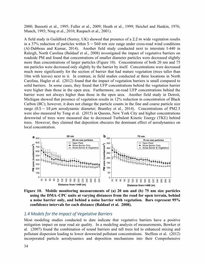
34

2000; Bussotti et al., 1995; Fuller et al., 2009; Heath et al., 1999; Heichel and Hankin, 1976; Munch, 1993; Ning et al., 2010; Raupach et al., 2001).

A field study in Guildford (Surrey, UK) showed that presence of a 2.2 wide vegetation results in a 37% reduction of particles within 5 560 size range under cross-road wind conditions (Al-Dabbous and Kumar, 2014). Another field study conducted next to interstate I-440 in Raleigh, North Carolina (Baldauf et al., 2008) investigated the impact of vegetative barriers on roadside PM and found that concentrations of smaller diameter particles were decreased slightly more than concentrations of larger particles (Figure 10). Concentrations of both 20 nm and 75 nm particles were decreased only slightly by the barrier by itself. Concentrations were decreased much more significantly for the section of barrier that had mature vegetation (trees taller than 10m with leaves) next to it. In contrast, in field studies conducted at three locations in North Carolina, Hagler et al. (2012) found that the impact of vegetation barriers is small compared to solid barriers. In some cases, they found that UFP concentrations behind the vegetation barrier were higher than those in the open area. Furthermore, on-road UFP concentrations behind the barrier were not always higher than those in the open area. Another field study in Detroit, Michigan showed that presence of vegetation results in 12% reduction in concentration of Black Carbon (BC); however, it does not change the particle counts in the fine and coarse particle size range (0.5 10 aerodynamic diameter; Brantley et al., 2014). Concentrations of PM2.5 were also measured by Tong et al. (2015) in Queens, New York City and higher concentrations downwind of trees were measured due to decreased Turbulent Kinetic Energy (TKE) behind trees. However, they claimed that deposition obscures the dominant effect of aerodynamics on local concentration.

Figure 10. Mobile monitoring measurements of (a) 20 nm and (b) 75 nm size particles

using the DMA–CPC units at varying distances from the road for open terrain, behind a noise barrier only, and behind a noise barrier with vegetation. Bars represent 95% confidence intervals for each distance (Baldauf et al. 2008).

1.4 Models for the Impact of Vegetative Barriers 

Most modeling studies conducted to date indicate that vegetative barriers have a positive mitigation impact on near road air quality. In a modeling analysis of measurements, Bowker et al. (2007) found the combination of sound barriers and tall trees led to enhanced mixing and pollutant dispersion leading to lower downwind pollutant concentrations. Steffens et al. (2012) incorporated particle aerodynamics and deposition mechanisms into their Comprehensive

35

Turbulent Aerosol Dynamics and Gas Chemistry (CTAG) model and examined the effects of vegetation on near-road air quality by comparing the results with measurements made in Chapel Hill, North Carolina by Hagler et al. (2012). They concluded that vegetation barriers affect the flow field and concentrations in three ways: 1) they increase vertical mixing by lofting some of the particles, 2) they lower wind speed and turbulence levels behind the vegetation barrier, and 3) they remove some particles by dry deposition. Tong et al. (2016) developed a model by incorporating Large Eddy Simulation (LES) into the CTAG model and evaluated the model performance against the dataset developed by Hagler et al. (2012). Then, they compared common vegetation barrier configurations near roadways to find the most effective configurations to guide urban planners. They concluded that a wide vegetation barrier with high Leaf Area Density (LAD) to increase deposition, and vegetation-solid barrier combinations work best as mitigation strategies.

1.5 Summary and Objectives for Current Study 

The observations on the impact of a vegetative barrier on near-road pollutant concentrations can be summarized by modeling it as a porous solid barrier. Then, part of the incoming flow goes through the barrier, and the remaining is lofted over the barrier. The part of the plume that is embedded in the lofted flow undergoes enhanced dispersion and thus is expected to have a lower concentration than in the absence of the barrier. The flow that goes through the barrier has turbulence levels (Steffens et al., 2012; Tong et al., 2015) that are smaller than those in the absence of the barrier because the porous vegetation reduces eddy sizes and thus increases turbulent dissipation close to the barrier. The turbulent levels recover to their upstream values at some distance from the barrier through entrainment of turbulent kinetic energy from the region above the barrier. This suggests that close to the barrier, the embedded plume undergoes less dispersion and thus results in concentrations that might be larger than those in open terrain. These features suggest that vegetation barriers could be less effective than solid barriers in reducing concentrations. However, vegetation can compensate for this by reducing the concentration of particles and gases in the air passing through the vegetation by deposition and impaction (Raupach et al., 2001). The entrapment of particles by windbreaks show that this removal is a function of the optical porosity of the vegetative barrier, leaf area index, the mass transfer coefficient, and the ‘bleed’ velocity through the barrier. Results from Steffens et al. (2012) suggest that the filtration effect of vegetation is small compared to the vertical mixing effect induced by solid barriers. Filtration can be increased by increasing the thickness of the vegetation barrier (Steffens et al., 2012). However, beyond a certain thickness there is no flow through the vegetation, which then effectively becomes a solid barrier.

The goal of this project is to provide information that can be utilized by the Air Resources Board (ARB) to provide state and local planners and decision makers with additional tools and information to inform their consideration of potential mitigation options for near roadway air pollution. Specific research objectives are to obtain field measurement data in California to evaluate the impacts of sound walls alone, and sound walls in combination with vegetation, on levels of traffic-related pollutants. The scientific objective of the study reported here is to reduce some of the uncertainty associated with our understanding of the impact of roadside vegetative barriers on dispersion of emissions from vehicles. We focus on the combination of solid and vegetative barriers, which is the most common configuration used along highways in California. The vegetation usually consisted of tall trees of varying density planted behind or in front a noise

36

barrier. The major questions that we seek to answer are: 1) Does the vegetative barrier increase or decrease the effectiveness of the solid barrier, 2) What is the magnitude of this effect, and how does it vary with the geometry of the barrier and atmospheric conditions.

The second objective is to develop a comprehensive data base that can be used for modeling studies in the future. Target pollutants include fine particulate matter (PM2.5), ultrafine particles, black carbon, oxides of nitrogen, carbon dioxide, and carbon dioxide, together with the variables that govern the impact of sound wall-vegetation combination barriers on near-road pollutant concentrations. These include the geometry of the sound wall and roadway, micrometeorology in the vicinity of the road, and traffic-activity patterns including traffic volume and speed, and fleet mix. The role of vegetation in deposition, dispersion and filtration of pollutants will be characterized using species and physical characteristics including optical porosity. We will capture the full range of micrometeorological variables that govern dispersion by making measurements at several sites during different times of the day in winter and in summer, as well as tower meteorological measurements. The objectives of the project were achieved through analysis of data collected in four field studies conducted in Encino, Riverside, Sacramento and Santa Monica during two seasons. Stationary measurements were collected 24 hours per day at Encino and Santa Monica and for more focused times during the day at Riverside and Sacramento. Mobile measurements were focused on daytime conditions in Encino and Sacramento and on the calm early mornings in Santa Monica. Some of the data collected at two sites in Riverside and Sacramento were interpreted using dispersion models.

 

2. Methods  

2.1 Descriptions of Sampling Sites 

A series of field sampling campaigns were carried out to collect near-freeway concentration data for UFPs (≤ 100 nm), PM2.5 (≤ 2.5 μm), and Black Carbon (BC) at Santa Monica, Encino and Sacramento. The three selected sampling sites included a site of I-10 freeway in Santa Monica, CA (figure 11); a site of I-101 freeway in Encino, CA (figure 12); and, a site of CA-99 freeway in Sacramento, CA (figure 13). Figure 11-13 present the aerial image of each sampling site. In each figure, four circles identify the continuous sampling sites. Different line schemes of the circles identify different combinations of soundwall and vegetation for each sampling location. For example, dashed green circles in Figure 11are continuous stationary sampling sites next to vegetation barrier along the shown study site of I-10. Similarly, the circles double-lined with solid black and dashed green represent the sampling locations with both soundwall and vegetation as shown in Figure 11. Finally, the target wind direction is indicated by the gray arrow.

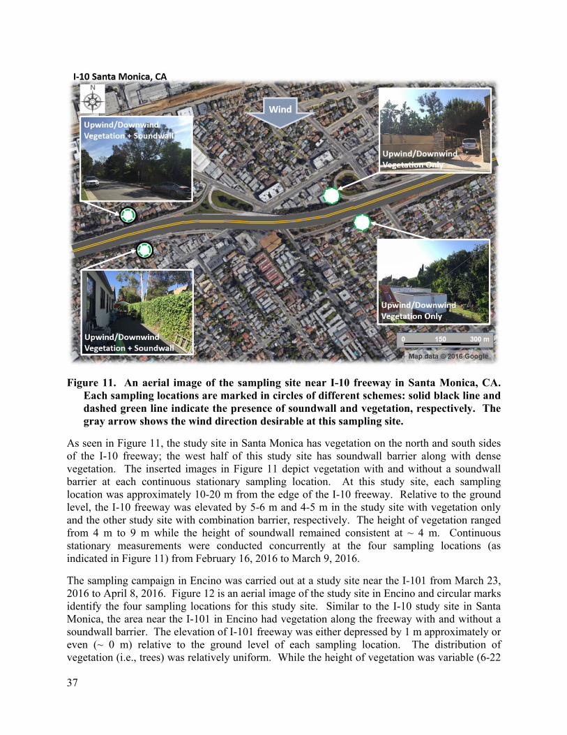
37

Figure 11. An aerial image of the sampling site near I-10 freeway in Santa Monica, CA. Each sampling locations are marked in circles of different schemes: solid black line and dashed green line indicate the presence of soundwall and vegetation, respectively. The gray arrow shows the wind direction desirable at this sampling site.

As seen in Figure 11, the study site in Santa Monica has vegetation on the north and south sides of the I-10 freeway; the west half of this study site has soundwall barrier along with dense vegetation. The inserted images in Figure 11 depict vegetation with and without a soundwall barrier at each continuous stationary sampling location. At this study site, each sampling location was approximately 10-20 m from the edge of the I-10 freeway. Relative to the ground level, the I-10 freeway was elevated by 5-6 m and 4-5 m in the study site with vegetation only and the other study site with combination barrier, respectively. The height of vegetation ranged from 4 m to 9 m while the height of soundwall remained consistent at ~ 4 m. Continuous stationary measurements were conducted concurrently at the four sampling locations (as indicated in Figure 11) from February 16, 2016 to March 9, 2016.

The sampling campaign in Encino was carried out at a study site near the I-101 from March 23, 2016 to April 8, 2016. Figure 12 is an aerial image of the study site in Encino and circular marks identify the four sampling locations for this study site. Similar to the I-10 study site in Santa Monica, the area near the I-101 in Encino had vegetation along the freeway with and without a soundwall barrier. The elevation of I-101 freeway was either depressed by 1 m approximately or even (~ 0 m) relative to the ground level of each sampling location. The distribution of vegetation (i.e., trees) was relatively uniform. While the height of vegetation was variable (6-22

38

m), the height of soundwall was consistent at ~ 4 m along the I-101 freeway at this study site. Continuous stationary data collections were conducted at ~ 15 m away from the edge of the freeway I-101.

Figure 12. An aerial image of the sampling site near I-101 freeway in Encino, CA. Each sampling locations are marked in circles of different schemes: solid black line and dashed green line indicate the presence of soundwall and vegetation, respectively. The gray arrow shows the wind direction desirable at this sampling site.

The third sampling site was located in northern California, near the CA-99 in Sacramento (See Figure 13). Continuous stationary data collection were conducted at this sampling site from June 17, 2016 to Jul 1, 2016. This study site had soundwall barrier of a consistent height (5 m) along the CA-99 freeway with and without vegetation. The height of the vegetation was relatively consistent (i.e., 16-17 m). Similar to the I-101 study site in Encino, the elevation of the CA-99 freeway was depressed slightly (by 0 – 1 m) relative to the ground level of continuous stationary sampling locations next to the freeway. All sampling instruments were located approximately 10-15 m away from the edge of the CA-99 freeway. Table 2 summarizes detailed information about the three study sites near the I-10 in Santa Monica, the I-101 in Encino, and the CA-99 in Sacramento.

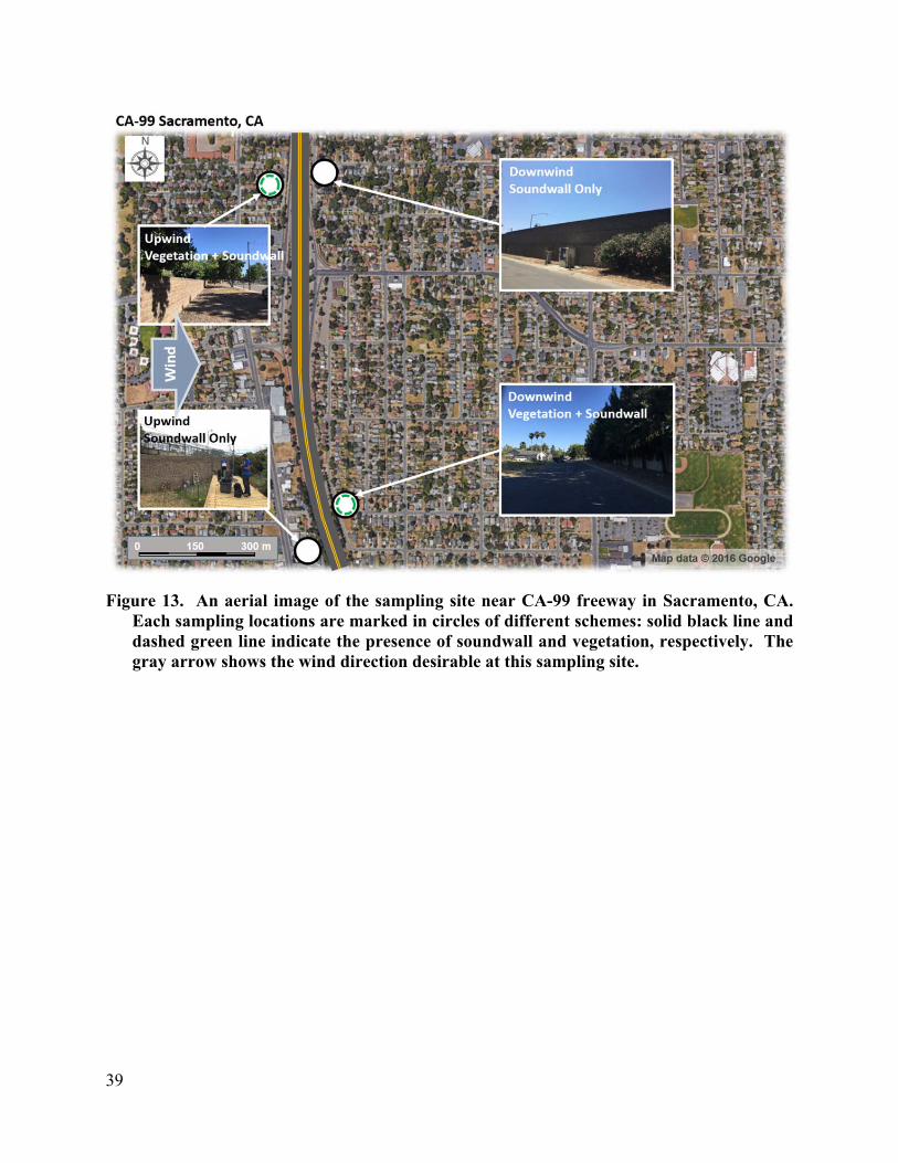
39

Figure 13. An aerial image of the sampling site near CA-99 freeway in Sacramento, CA. Each sampling locations are marked in circles of different schemes: solid black line and dashed green line indicate the presence of soundwall and vegetation, respectively. The gray arrow shows the wind direction desirable at this sampling site.

40

Table 2. A summary of three study sites near the I-10 freeway in Santa Monica, the I-101 freeway in Encino, and the CA-99 freeway in Sacramento.

Study Site I-10 Santa Monica, CA(34°01'40"N 118°27'05"W)

I-101 Encino, CA (34°10'9"N 118°31'46"W)

CA-99 Sacramento, CA(38°32'28"N 121°28'23"W)

Riverside

(34°58'15"N 117°19'45"W)

Experimental Configuration Vegetation Only (VO)

Vegetation with Soundwall (VW)

Vegetation Only (VO)

Vegetation with Soundwall (VW)

Soundwall Only(WO)

Vegetation with Soundwall (VW)

Soundwall only

Nearby Intersection Pearl St. & Granville Ave.

Urban Ave. & Dorchester Ave.

Killion St. & New Castle Ave.

Killion St. & Encino Ave.

32nd St. & 19th Ave.

32nd St. & 9th Ave.

UCR parking lots 5, 6, 30.

Freeway Elevation Elevated by 5-6 m

Elevated by 4-5 m

0 m

(Depressed by 1 m)

0 m

(Depressed by 1 m)

0 m Elevated by 1 m

0 m

Vegetation Height 5-8 m 4-9 m 6-11 m 13-22 m None 16-17 m None

Soundwall Height None 4 m None 4 m 5 m 5 m 5 m

Sampling Distance to Freeway for continuous particle measurements

15 m 15 m 15 m 15 m 10 m 10 m

5-150 m

Stationary Sampling Period February 16 – March 9, 2016

(Continuous 24-h sampling)

March 23 – April 8, 2016

(Continuous 24-h sampling)

June 17 – July 1, 2016

(Variable time of a day; sampling conducted when the wind direction was 270 ± 45°.)

July 2014 – March 2015

(Variable time of the day)

Mobile Sampling Period*

5 days between October 1-9,205 5 days between February 22- March 9,2016

5 days between March 25- April 7,2016

7 days between June 20- June 30,2016

None

*Detailed times are shown in Table .

41

2.2 Traffic flow and Overview of Wind Data 

Table 2 summarizes the wind data and the traffic flow with truck flow (% in parenthesis) observed during sampling campaigns at each study site. Traffic flow data near the sampling sites were reported from two nearby traffic sensors of the CalTrans Performance Measurement System (PeMS) (CalTrans 2016). The traffic flow data used in this study were obtained from the PeMS traffic sensors reporting 99% or greater observations in both directions (e.g., north- and southbound), except for the westbound traffic sensor (PeMS ID: 717513) of the I-101 freeway in Encino. This traffic sensor reported 80%. All traffic sensors were located within the study area of freeway or at least within 2-km distance to a sampling location. When there were on-ramps/off-ramps present between the selected main line sensor and the measurement transect, either measured traffic flow rates from on-ramp/off-ramp sensors or historical traffic data was used to calculate the best estimate of the traffic flow at each transect. All traffic data had 5 min time resolution.

Meteorological variables were measured with Campbell Scientific CSAT3 3-D (three dimensional) sonic anemometers. It can measure horizontal wind velocity at 1 mm/s and vertical wind velocity at 0.5 mm/s resolution. It also records temperature with resolution of 0.025°C. Campbell Scientific CR1000, CR3000, and CR5000 data loggers were used to record the data at 1HZ frequency. Sonic anemometers were powered by deep cycle marine batteries. Wind data (i.e., intensity and direction) were collected using 3-D ultrasonic anemometers during sampling near the I-10 in Santa Monica and the CA-99 in Sacramento. For the data collection at the I-101 study site in Encino, the wind data were obtained from a 2-D ultrasonic anemometer located at the weather station (ID: KVNY) at Van Nuys Airport located at 5 km NW of the study site. This weather station is in part of the Automated Surface Observing Systems (ASOS). Table 2 provides a summary of traffic flow and wind conditions during the three sampling campaigns in Santa Monica, Encino, and Sacramento. Here we analyzed the data collected only under a specific range of wind directions at each site. The data provided in Table 2 are the arithmetic averages of the 1-min data collected under the desirable wind conditions. For analyses presented here, data were divided into approximately perpendicular (within ± 45 ° of the perpendicular to the freeway center-line, and in a direction such that the specified side was downwind) and approximately parallel (within ± 45 ° of the parallel to the freeway center-line) based on wind direction.

42

Table 2. A summary of traffic flow and wind speed data from three sampling sites. The data are given in arithmetic averages and one standard deviations from all data collected under the specific wind direction as noted. This data corresponds to continuous stationary data collected at continuous stationary sampling sites.

Study Sites I-10 Santa Monica, CAPeMS ID: 737249 (EB) & 763490 (WB)

I-101 Encino, CA PeMS ID: 717511 (EB) & 717513 (WB)

CA-99 Sacramento, CAPeMS ID: 312562 (NB) & 318858 (SB)

Desirable

Wind Direction

Northerly Wind(309 ± 45°)

Southerly Wind(150 ± 45°)

Northerly Wind (0 ± 45°)

Westerly Wind (270 ± 45°)

Traffic Flow (Truck Flow in %)

400 ± 289 veh./5-min (1 ± 1%)

638 ± 258 veh./5-min (1 ± 1%)

1221 ± 195 veh./5-min (5 ± 2%)

752 ± 71 veh./5-min (8 ± 3%)

Wind Speed 0.88 ± 1.59 m/s 0.79 ± 1.55 m/s 1.10 ± 0.75 m/s 1.57 ± 0.50 m/s

Wind Direction Northerly Wind(202 ± 157°)

Southerly Wind(150 ± 27°)

Northerly Wind (15.10 ± 21.35°)

Westerly Wind (276.68 ± 22.96°)

Figure 14 shows the diurnal change of traffic flow and wind speed under the given range of wind direction near I-10 in Santa Monica. The traffic flow on the I-10 freeway reached up to ~ 1100 vehicles per 5 minute (veh./5-min) during the morning rush hours and remained high until the afternoon rush hours; whereas, the minimum traffic volume was as low as ~ 30 veh./5-min overnight. For the studied site of the I-10 freeway, traffic flow had relatively low heavy-duty truck flow that was ~ 1% of the total daily average. At this site, northerly or southerly wind conditions provided upwind and downwind conditions that comply with the given experimental design for this study site. There was relatively low wind speed of 0.88 (±1.59) m/s and 0.79 (±1.55) m/s under northerly (345 ± 45°, in Figure 14a) and southerly (165 ± 45°, Figure 14b) wind conditions, respectively.

Figure 15 shows the diurnal changes of traffic flow and wind speed under the wind direction, as specified, at the study site near the I-101 in Encino. The study site in Encino had traffic flow reaching up to ~1300 veh/5-min that is slightly higher than the study site near the I-10 in Santa Monica. The I-101 study site in Encino had a desirable range of wind direction at 0 ± 45 ° (i.e., northerly wind) as the I-101 freeway was running west to east. In Sacramento, the CA-99 was running from north to south; thus, the desirable wind direction became westerly wind direction (270 ± 45 °). Figure 15 provides the diurnal changes of wind speed under the given range of wind direction that this study aimed to conduct data collection. The average wind speed was 1.00 (± 0.65) m/s near the I-101 site in Encino and 1.57 (± 0.50) m/s near the CA-99 in Sacramento. Note that the wind speed data collected in Encino and Sacramento were higher than

43

that from Santa Monica. The study site in Sacramento also had slightly (~ 200 veh./5-min) lower traffic flow at the peak traffic hours than the I-10 in Santa Monica.

Figure 14. A time-series of diurnal traffic flow (veh./5-min, dark gray) and wind speed (m/s, light gray) under (a) Northerly Wind (WD ≥ 300 ° or WD < 30 °) and (b) Southerly Wind (120 ≤ WD < 210 °) conditions at the I-10 sampling site in Santa Monica, CA.

44

Figure 15. A time-series of diurnal traffic flow (veh./5-min, dark gray) and wind speed (m/s, light gray) at two sampling sites: (a) I-101 in Encino and (b) CA-99 in Sacramento.

45

2.2.1 Detailed Traffic Analysis 

Traffic flow rate data was retrieved from the Caltrans Performance Measurement (PeMS system). For each site, for each traffic flow direction, the closest main line sensor on the freeway for each measurement transect was used, if the senor had >99% observation rate (except for one sensor at the Encino site with an 80% observation rate and one sensor at the Sacramento site with 75% observation rate). All main line traffic sensors were within 2 km from the sites. When there were on-ramps/off-ramps present between the selected main line sensor and the measurement transect, either measured traffic flow rates from on-ramp/off-ramp sensors or historical traffic data was used to calculate the best estimate of the traffic flow at each transect. All traffic data had 5 min time resolution.

Santa Monica site: At the Santa Monica site, in the fall session, the west-bound (WB) and east-bound (EB) traffic flows at the two transects were calculated using the main line and on-ramp/off-ramp sensor noted below (Figure 16). The yellow stars indicate the stationary measurement/ mobile measurement transect locations. These sites are Granville (left) and Dorchester (right). In the equations below, Granville WB/EB and Dorchester WB/EB represent traffic flow on the freeway calculated at each site using the observed traffic counts from the mainline sensors (Centinela, Pico and Cloverfield) and on/off ramps.

Granville WB= Pico (+ correction) + 2 × off-ramp Bundy (sample data) Granville EB= Centinela + on-ramp Centinela + on-ramp Bundy (sample data) Dorchester WB= 20th + off-ramp Cloverfield (sample data) Dorchester EB= Cloverfield + on-ramp Cloverfield

Figure 16. The location of PeMS sensors used in the traffic flow calculations at the Santa Monica site. The yellow stars note the location of the measurement transects. The green circles show the main line sensors used in the calculation. Green arrows show the ramps with data available and red arrows show the ramps with no data available.

The main line sensors at Dorchester had poor correlation with other mainline sensors adjacent to them. Hence data from Dorchester main line sensors was not used in the traffic flow calculations. Although WB Centennial sensor was closer to the Dorchester transect, data was not

20th (WB) 

Cloverfield

Centinela (EB) 

Pico (EB)Centinela (WB) 

Bundy

46

available for fall session. Hence the WB 20th sensor was used together with a correction for Cloverfield off-ramp to estimate the WB flow at Dorchester. The closest WB sensor for the Granville transect was the Pico sensor. The WB sensors at Centinela and Pico showed discrepancies. Information was not available to assess the accuracy of each sensor. Therefore, a correction for the WB Pico sensor was calculated as follows. First the mean flow value of the Centinela and Pico sensors was the calculated from a sample data set out side measurement period. Then the flow difference between Pico sensor and the calculated mean was averaged over 5 weekdays to obtain the correction. There are two off-ramps to Bundy Dr. in between the Pico sensor and Granville transect. WB Bundy off-ramp data was not available for the measurement period. A sample data set available outside of the measurement days, were averaged over 5 weekdays to obtain the values used in the above calculations. Furthermore, we assumed that both WB Bundy off-ramps have had equal traffic flow.

At the Santa Monica site, in the winter session, the traffic flow at the two transects were calculated using the following sensors (Figure 16):

Granville WB=mean (Centinela and Pico) + 2 × off-ramp Bundy (sample data) Granville EB= Cloverfield + on-ramp Cloverfield - off-ramp Cloverfield + on-ramp Centinela (sample data) + on-ramp Bundy (sample data) Dorchester WB=mean (Centinela and Pico) + on-ramp Centinela Dorchester EB= Cloverfield + on-ramp Cloverfield

The WB sensors at Centinela and Pico showed discrepancies. Since information was not available to assess the accuracy of each sensor, the mean flow value of these two sensors was used in the calculations. For Bundy and Centinela ramps, sample data sets available outside of the measurement days were averaged over 5 weekdays to obtain the sample data values used in the above calculations.

Figure 17 shows the 30 min mean of the traffic flow in both directions at each measurement transect, together with the standard deviation of the mean, at the Santa Monica site. The day-to-day variation is in the traffic flows was very small. Averaged over the measurement period and all measurement days, the freeway traffic flow near Granville Ave. was 2.5 % higher than the freeway traffic flow near Dorchester Ave. in the fall session and 4.9 % higher than the freeway traffic flow near Dorchester Ave. in the winter session.

47

Figure 17. The diurnal traffic flow variation on I 10 at Santa Monica site, during (a) fall and (b) winter measurement sessions. The 30 min mean of the traffic flow in both directions at each measurement transect (color symbols) and the standard deviation of the mean. Different symbols indicate different measurement days.

Encino site: At the Encino sites, sensors were not available for several on and off ramps in between the sites. Hence, we use a single traffic flow value for both transects at this site. The west-bound (WB) and east-bound (EB) traffic flows at the two transects were calculated using the main line sensors noted below (Figure 18).

Encino/ Zelzah WB= Reseda Encino/ Zelzah EB= Burbank + on-ramp Burbank

Figure 18. A schematic showing locations of PeMS sensors used in the traffic flow calculations at the Encino site. The yellow starts note the location of the measurement transects. The green circles show the main line sensors used in the calculation. Green arrows show the ramps with data available and red arrows show the ramps with no data available.

Figure 19 shows the 30 min mean of the traffic flow in both directions, together with the standard deviation of the mean, at the Encino site. The day time traffic flow at Encino shows larger day-to-day variation compared to the early-morning traffic flow at Santa Monica.

(a (b)

Dorchester Ave. Granville Ave.

Burbank (EB)

Reseda (WB) 

48

Figure 19. The diurnal traffic flow variation on I 101 at Encino site. The 30 min mean of the traffic flow in both directions and the standard deviation of the mean. Different symbols indicate different measurement days.

Sacramento site: At the Sacramento site, the north-bound (NB) and south-bound (SB) traffic flows at the two transects were calculated using the main line and on-ramp/off-ramp sensor noted below (Figure 20).

19th NB = 21st ave (NB) 19th SB= 21st ave (SB) 9th NB= 12st ave (NB) + on-ramp 12th 9th SB= 12st ave (SB)+ off-ramp 12th

Figure 20. A schematic showing locations of PeMS sensors used in the traffic flow calculations at the Sacramento site. The yellow starts note the location of the measurement transects. The green/yellow circles show the main line sensors used in the calculation. Green arrows show the ramps with data available.

21st

12st  

49

Figure 21 shows the 30 min mean of the traffic flow in both directions at each measurement transect, together with the standard deviation of the mean, at the Sacramento site. The daytime traffic flow shows large day-to-day variation, similar to the Encino site. Averaged over the measurement period and all measurement days, the freeway traffic flow near 19th Ave. was 4 % higher than the freeway traffic flow near 9th Ave.

Figure 21. The diurnal traffic flow variation on SR 99 at Sacramento site. (a) The 30 min mean of the traffic flow in both directions at each measurement transect (color symbols) and the standard deviation of the mean. Different symbols indicate different measurement days. (b) The 30 min mean of the traffic flow in both directions, averaged of all measurement days, and the standard deviation of the mean.

 

2.2.2 Encino Meterological Measurements 

A 3D sonic anemometer was installed north of the I-101 freeway to characterize the dominant winds in preparation for the Encino campaign. It was installed on the roof of a residence at a height of 5 m, and was operated from February 17th 2016 to March 9th 2016.

(a) (b)

50

Figure 22- Location of installed sonic anemometer and Van Nuys meteorological station during Encino field study

Unfortunately, the data logger connected to the sonic anemometer failed during the period of the Encino field study, March 15th to April 15th. It became necessary to construct a data set from other sources that could be used to interpret the concentrations measured during the field study. The first step in doing so was to establish similarity between the wind information from the alternate source and the sonic measurements made at the Encino site when the data logger was working.

Discussions among the project team lead to the selection of the following data set as the alternate source: 1-min averaged meteorological data (Automated Surface Observing System, ASOS) reported by National Oceanic and Atmospheric Administration (NOAA) from the Van Nuys weather. The interpretation of the concentration measurements from the mobile platform relied on wind direction, which was used to determine the time during which measurements were made downwind of the freeway. We focused on this variable by comparing the wind directions measured by the sonic anemometer with those measured by ASOS for several days. The comparisons of time series from the two datasets from Feb. 17th 2016 – Feb. 28th 2016 are shown in Figure 23. This figure provides a visual representation of the good agreement between the wind directions from the two sources.

51

52

Figure 23- Time series of wind direction data from Feb. 17th 2016– Feb. 28th 2016 collected by the sonic anemometer ( ) and by ASOS ( ).

We also established similarity between the wind directions from the two sources by comparing histograms of the wind directions binned in 90° intervals around northerly, easterly, westerly, and southerly directions. The 1 minute averaged winds used to construct the histograms covered the interval, 9 am – 3 pm, corresponding to the sampling period of the mobile platform. The histograms, shown in Figure 24, indicate that the sonic anemometer wind direction is northerly

53

36% of the time, which is close to 32%, the frequency of northerly wind directions from the ASOS data.

Figure 24. Frequencies in each wind direction based on a) sonic anemometer and b) ASOS data.

The wind roses from the two sites are also similar as seen in Figure 25.

a) b)

Figure 25. a) Wind rose for the data collected by Van Nuys sonic anemometer from February 17th to February 29th. b) Wind rose for the data collected by Van Nuys meteorological station from February 17th to February 29th 2016.

In order to estimate the reliability of using the ASOS data to determine whether the mobile platform was downwind of I-101, we determined the conditional probability that the sonic anemometer wind direction was northerly given that the ASOS wind direction was northerly. An

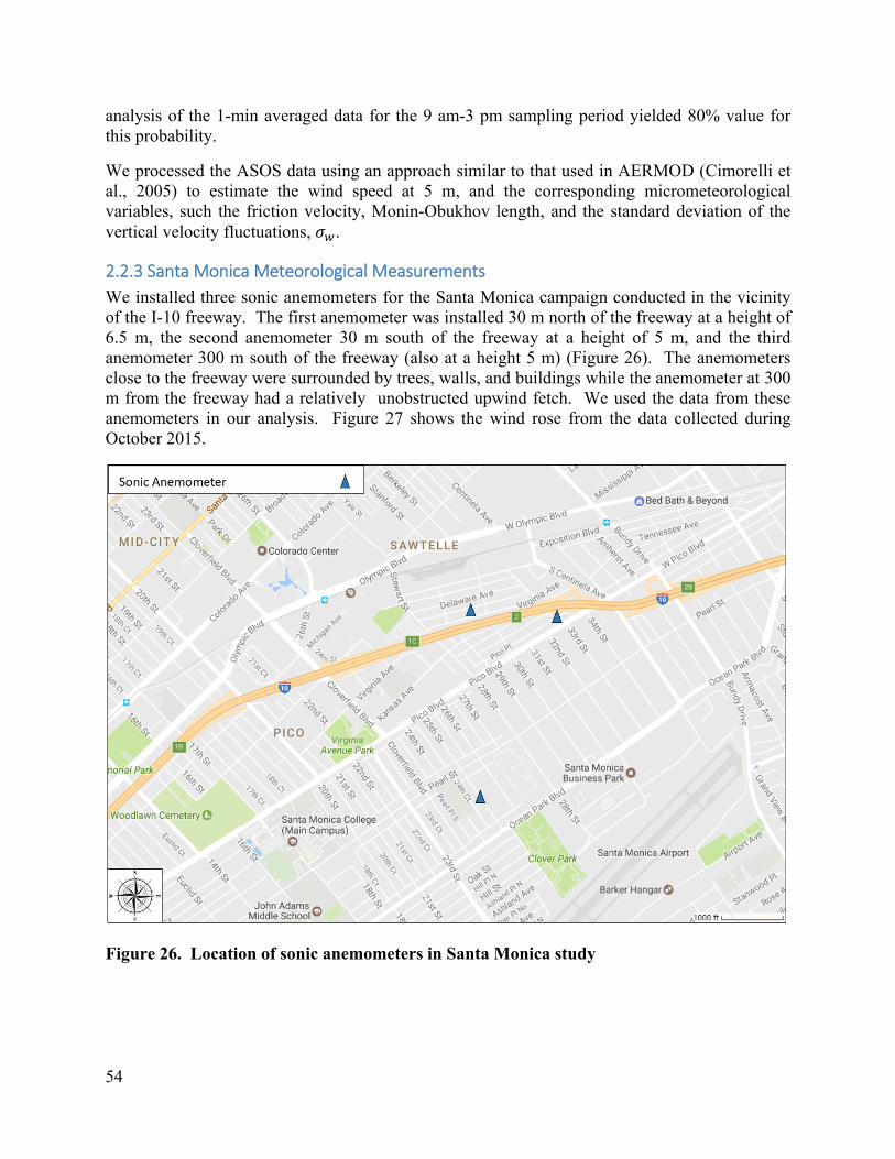
54

analysis of the 1-min averaged data for the 9 am-3 pm sampling period yielded 80% value for this probability.

We processed the ASOS data using an approach similar to that used in AERMOD (Cimorelli et al., 2005) to estimate the wind speed at 5 m, and the corresponding micrometeorological variables, such the friction velocity, Monin-Obukhov length, and the standard deviation of the vertical velocity fluctuations, .

2.2.3 Santa Monica Meteorological Measurements 

We installed three sonic anemometers for the Santa Monica campaign conducted in the vicinity of the I-10 freeway. The first anemometer was installed 30 m north of the freeway at a height of 6.5 m, the second anemometer 30 m south of the freeway at a height of 5 m, and the third anemometer 300 m south of the freeway (also at a height 5 m) (Figure 26). The anemometers close to the freeway were surrounded by trees, walls, and buildings while the anemometer at 300 m from the freeway had a relatively unobstructed upwind fetch. We used the data from these anemometers in our analysis. Figure 27 shows the wind rose from the data collected during October 2015.

Figure 26. Location of sonic anemometers in Santa Monica study

55

Table 3. Overview of measurement in Santa Monica

Location of sonic anemometer

Measurement Dates

300m south of the freeway 5/11/2015-6/4/2015, 9/25/2015-10/25/2015, 8/4/2015-9/4/2015, 2/17/2016-2/23/2016

30m south of the freeway 5/11/2015-6/4/2015, 9/25/2015-10/16/2015

30m north of the freeway 5/11/2015-6/4/2015, 9/25/2015-10/16/2015

Figure 27. Wind rose for the data collected at Santa Monica during October 2015

 

56

2.2.4 Sacramento Meteorological Measurements 

The wind rose (Figure 30) derived from winds measured at the Sacramento Executive Airport shows that the dominant wind direction during the daytime is from the southwest. During the night, the winds are light from the north.

Figure 28. Instrument locations in Sacramento site.

The field study was conducted at two barrier sites (Figure 28). The first site has one 5 m barrier extending over 500 m on the east side of the highway. The other site has a barrier of the same height with tall trees planted behind. The vegetation is a row of pine trees planted next to the barrier extending over 200 m along the highway. The height of the trees is 15-18 meters. The freeway is at the same level behind the barriers at both sites.

57

a)

b)

Figure 29. a) view of wall vegetation barrier. b) view of barrier and downwind anemometer behind it.

At both locations, the areas downwind of the barriers are residential with one story houses. There are also streets behind the barriers at both locations, which made it possible to make measurements within 10 m from the barriers.

58

Figure 30. Wind rose from Sacramento Executive Airport meteorological station during June 2016.

In Sacramento, another set of anemometers were located at west side of the freeway at a local resident house next to the CA-99 to measure temperature and wind velocities. One of the anemometers was used as a backup unit. Since the wind was blowing from the southwest most of the time, measurements at this location were considered background. Both anemometers were installed on a pole at 5 m above ground level (AGL).

A total of four sonic anemometers were installed during the study. Two sonic anemometers were located at west side of the freeway at a local resident house next to the highway 99 to measure temperature and wind velocities. One of the anemometers was used as a backup unit. Since the wind was blowing from the southwest most of the time, measurements at this location are considered as background. The anemometers were installed on a pole at 5 m above ground level (AGL).

Another sonic anemometer was installed at each of the downwind sampling locations to measure the effects of the solid and the solid-vegetation barriers on wind characteristics and turbulence levels. The sonic anemometers were installed on poles at 2.5 m high above the ground and at 4 m behind downwind of the barrier.

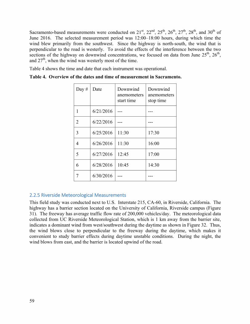
59

Sacramento-based measurements were conducted on 21st, 22nd, 25th, 26th, 27th, 28th, and 30th of June 2016. The selected measurement period was 12:00–18:00 hours, during which time the wind blew primarily from the southwest. Since the highway is north-south, the wind that is perpendicular to the road is westerly. To avoid the effects of the interference between the two sections of the highway on downwind concentrations, we focused on data from June 25th, 26th, and 27th, when the wind was westerly most of the time.

Table 4 shows the time and date that each instrument was operational.

Table 4. Overview of the dates and time of measurement in Sacramento.

Day # Date Downwind anemometers start time

Downwind anemometers stop time

1 6/21/2016 --- ---

2 6/22/2016 --- ---

3 6/25/2016 11:30 17:30

4 6/26/2016 11:30 16:00

5 6/27/2016 12:45 17:00

6 6/28/2016 10:45 14:30

7 6/30/2016 --- ---

2.2.5 Riverside Meteorological Measurements 

This field study was conducted next to U.S. Interstate 215, CA-60, in Riverside, California. The highway has a barrier section located on the University of California, Riverside campus (Figure 31). The freeway has average traffic flow rate of 200,000 vehicles/day. The meteorological data collected from UC Riverside Meteorological Station, which is 1 km away from the barrier site, indicates a dominant wind from west/southwest during the daytime as shown in Figure 32. Thus, the wind blows close to perpendicular to the freeway during the daytime, which makes it convenient to study barrier effects during daytime unstable conditions. During the night, the wind blows from east, and the barrier is located upwind of the road.

60

Figure 31. Map of the selected site in Riverside. Adapted from Google Earth.

Figure 32. Wind rose from UC Riverside meteorological station and freeway direction at barrier site during February 2015.

The barrier, which is 3 m away from the edge of the road, is 4.5 m high and 1 km long. There are three lanes and one High Occupancy Vehicle (HOV) lane on the north bound side and four lanes and one HOV lane on the south bound side of the freeway. There is an entrance to the north bound lanes and an exit on the south bound side of the freeway. The lanes are 3.5 m wide

61

and the median is 10 m across. The freeway is at the same level as the adjacent streets. There is no major source of pollution within a 3.5 km radius of the barrier site except the freeway. The heading of the freeway is 140°. Therefore, the wind direction perpendicular to the freeway is 230° true to north. Two parking lots are located behind the barrier, which provide convenient locations for sampling.

The largest obstacles in the parking lots downwind of the barrier are widely scattered trees. There are no other major obstacles within 170 m of the barrier. A 2-lane street, West Campus Drive, runs parallel to the freeway between the parking lots. The street is mainly used to access the parking lots and the traffic is mainly passenger cars travelling during the morning hours, 08:00-10:00, and in the evening, 16:00-18:00. Another parking lot extends for 300 m west of the freeway. There is no major obstacle in this parking lot and trees are sparser and shorter than in the eastside parking lots.

Two 3-D sonic anemometers were employed to measure upwind and downwind flow characteristics. A sonic anemometer was attached to a light post on the upwind side of the freeway (parking lot 30; assuming wind is WSW) at 4 m height above ground level (AGL) to capture upwind flow characteristics. The UC Riverside Community Garden is located on the west side of the anemometer, which ensured the absence of any major obstacles to upwind wind flow. Another sonic anemometer was attached to a light post within the wake region behind the barrier at 4 m AGL to record flow characteristics behind the barrier.

Information regarding traffic flow on each lane of the freeway was downloaded from the CalTrans Performance Measurement System (www.pems.dot.ca.gov). The detectors record the number of cars and trucks separately.

The wind direction during all the tests was within 45° of perpendicular to the freeway. The wind direction perpendicular to the freeway is 230° true to north. The meteorological conditions used to analyze the data correspond to the upwind 3-D sonic anemometer, which are shown in Table 6. The air quality data, micrometeorological data, and traffic data were averaged over 30-minute periods for analysis.

Table 5. Meteorological conditions in Riverside study.

Test # of data points

Mean Monin-Obukhov Length (m)

Mean Wind Direction (deg true N)

Mean Wind Speed (

Mean Friction Velocity (

Cloud Cover

1 10 -11.5 254° 2.72 0.31 Clear

2 7 -15.7 256° 1.37 0.17 Clear

3 9 -9.1 238° 1.00 0.14 Clear

4 10 -5.8 254° 1.14 0.14 Clear

5 9 -38.8 238° 2.45 0.44 Mostly Cloudy

6 9 -43.0 268° 2.83 0.47 Partly Cloudy

62

Tests 1 through 4 were conducted in unstable conditions. Winds were moderate during test 1 and very light during tests 2, 3, and 4. No major variability in wind direction was observed during the first 4 tests and the wind directions were almost always favorable with respect to the freeway orientation. Skies were clear during the first 4 tests.

The surface boundary layer was unstable even during tests 2, 3, 4, which were conducted in the late evening and night when the sun had set. Tests 5 and 6 were conducted in near neutral conditions. Winds were moderate and the wind direction was steady. Wind directions were almost always favorable during these two tests. Skies were mostly cloudy in test 5 and partly cloudy in test 6.

The meteorological data measured by the UCR meteorological station (Figure 32) were consistent with the on-site sonic anemometer data, which indicated that the upwind anemometer was not affected by local obstacles.

2.3 Continuous Stationary Measurements 

2.3.1 Particle size distributions, PM2.5 and black carbon 

Several concurrent measurements were conducted at 3-4 private residences located at each study site. Four sets of Scanning Mobility Particle Spectrometers (SMPSs) were deployed to measure the total number particle concentrations and particle size distributions in the size range of 10-289 nm. All four sets of SMPSs had the same model Electrical Classifier (EC, model 3080, TSI Inc., Shoreview, MN) with the same model Differential Mobility Analyzer (DMA, model 3081, TSI Inc., Shoreview, MN). For four sets of SMPSs, during the sampling campaigns in Santa Monica and Encino, TSI Condensation Particle Counter (CPC) models 3022 and 3788 were deployed to the upwind locations (i.e., upwind locations with combination barrier and vegetation only, respectively) and TSI CPC models 3785 and 3786 were deployed to the downwind locations (i.e., downwind locations with combination barrier and vegetation only, respectively). During the sampling campaign in Sacramento, two units of the same model CPC (TSI model 3022) were deployed to two upwind locations. At two downwind locations, the CPC models 3785 and 3788 were deployed and periodically exchanged between two downwind sampling locations that have soundwall barrier and combination barrier. Data corrections were made with correlation data acquired from linear regressions of instrument collocation data collected before and after each sampling campaign. The applied scanning and retrace times were 100 and 20 s, respectively.

In addition, three DustTraks were used to concurrently measure PM2.5 mass concentrations at one upwind location (model 8532, TSI Inc., Shoreview, MN) and two downwind locations (model 8520, TSI Inc., Shoreview, MN) that have different combinations of vegetation and soundwall barriers near I-10 in Santa Monica and I-101 in Encino. Two DustTraks (model 8520, TSI Inc., Shoreview, MN) were deployed to measure the PM2.5 concentrations at two downwind locations near CA-99 in Sacramento. Similarly, two Aethalometers (models AE-33 and AE-42, Magee Scientific Co., Berkeley, CA) were deployed to measure BC mass concentrations downwind of freeway. Linear regression of collocation data was conducted to correct any potential error that can occur from the use of different models or among different units of the same model. In addition, PM2.5 data were also corrected for the known discrepancy between optical

63

measurements (i.e., DustTrak, TSI model 8520) and gravimetric measurements. During collocation, the instruments were operated in a temperature-controlled environment (i.e., 17-23 °C) that was within the temperature range (i.e., 10-35 °C) of instrument operation. All instruments were calibrated prior to the deployment for the field sampling campaign, and data logging intervals were set to 1 min.

2.3.1.1 Riverside Particle Measurements 

Ultrafine particles (UFPs) were used as the tracer in this study for several reasons. First, because they have adverse health effects (Pope III 2002), the levels of UFP concentrations next to a major highway are of public interest. Second, their concentrations next to major highways are well above background levels, and can be measured continuously with readily available instruments. Gidhagen et al. (2005) and Zhang et al. (2004) show that at the 100 m scale being considered here, deposition and coagulation play a minor role relative to turbulent dispersion in reducing particle number concentrations. Thus, UFP can be treated as a passive tracer by using particle number concentrations to characterize dispersion. One major problem with using UFP as a tracer is that UFP emission factors from vehicles are highly uncertain (Kumar et al., 2011; Morawska et al., 2008). Thus, it is necessary to treat the emission factor as an unknown whose value is obtained by fitting model estimates to measurements. This process is discussed in more detail in a later section.

Fifteen tests were conducted on different days and at different times of day from July 2014 to May 2015 but due to the malfunction of instruments and unfavorable meteorological conditions, only six tests were selected for analysis. Table 7 shows the dates and duration of measurements. The total duration of the 6 tests is 27 hours.

Table 6. Overview of dates and duration of measurements in Riverside.

Test UFP measurement dates Time of Measurement

1 07/22/2014 12:00-17:00

2 08/11/2014 20:00-23:30

3 08/18/2014-08/19/2014 20:00-00:30

4 08/19/2014-08/20/2014 20:00-01:00

5 04/07/2015 12:30-17:00

6 05/05/2015 14:00-18:30

 

UFP number concentrations were measured using TSI Condensation Particle Counters (CPC), Model 3022A. The cutoff size of these CPCs is 7 nm. The measured concentrations ranged from5 10 10 particles/cm3. The accuracy within this range of concentrations is 10%. The measurements of CPC concentrations were stored on a custom-designed data logger.

64

Several CPCs were used to measure background UFP concentrations and downwind UFP concentrations at several downwind distances. A CPC was placed at the upwind side of the freeway (assuming that the wind is blowing WSW) to measure background UFP number concentrations. The rest of the CPCs were deployed behind the barrier (Figure 33). The downwind CPCs were placed at least 250 m away from the barrier edge to avoid barrier edge effects. CPC locations were changed from one test to another to avoid any systematic bias in measurements. The background concentrations were subtracted from the downwind concentrations to estimate contributions from vehicles on the highway.

Figure 33. Approximate location of instruments in Riverside site.

2.3.2 Passive Measurements of NO and NO2  

Twelve Ogawa passive NO/NOx samplers (Ogawa Inc., Pompano Beach, FL) were deployed during each of three campaigns at Santa Monica, and at Sacramento and Encino. The samplers, which are light and relatively inexpensive, were attached at heights of 2-3 m above ground level to available structures at residents’ houses and on trees, lamp posts or street signs at the beginning of each campaign, At the end of the campaign, they were recovered, sealed and sent to RTI International (Research Triangle, NC). for analysis. Data were corrected for any difference that can occur from relative humidity and temperature. NO2 concentration was determined from subtraction of the time-averaged NO and NOx measurements (i.e., NO2 = NOx – NO).

65

2.3.3 Difference‐in‐Differences Analysis  

Spatial difference-in-differences (DID) analyses were conducted for the data collected at four continuous stationary sampling locations at each sampling site. The DID analyses aimed to determine the effectiveness of an additional road-side barrier (i.e., vegetation or soundwall).

First, the downwind-upwind differences (i.e., the downwind concentration subtracted by the upwind concentration) were estimated from a pair of upwind and downwind datasets. Upwind and downwind sampling locations typically share the same regional background level of air pollution. Thus, the difference calculation eliminates the contribution of regional background to the downwind measurements. Therefore, the estimated difference represents the impact of traffic emissions from the freeway. Mann-Whitney U-test was conducted to determine the statistical significance of the differences observed from the measurements. For comparison at each sampling site, the paired data collection was conducted concurrently at both study sites with different configurations of vegetation and soundwall barriers. For example, the downwind-upwind difference found in the study site with vegetation only was noted as dVO, and the difference found in the study site with vegetation and soundwall is noted as dVW. Similarly, the difference found in the study site with soundwall only is noted as dWO.

Then, DID values were estimated from another subtraction between the differences estimated at two study sites that have different vegetation-soundwall configurations. For I-10 in Santa Monica and I-101 in Encino, while both study sites have vegetation along the freeway, one study site has a soundwall barrier (i.e., dVW), but the other study site does not have a soundwall barrier (i.e., dVO). Thus, DID is estimated as follows: DID = dVO – dVW. Therefore, the estimated DID values indicate the effects of an additional soundwall barrier in the existing vegetation near the I-101 in Encino. In comparison, the study site near the CA-99 in Sacramento has soundwall barrier along the freeway with vegetation (i.e., dVW) and without vegetation (i.e., dWO). Accordingly, DID is estimated as follows: DID = dWO – dVW which shows the effects of an additional vegetation barrier on the existing soundwall barriers near the CA-99 study site in Sacramento.

In summary, the DID analyses in this study aimed to determine the effectiveness of an additional barrier (i.e., vegetation or soundwall) for reducing particulate air pollution near major freeways.

2.4 Mobile Measurements 

2.4.1 Mobile Measurements Description 

When available, mobile measurements were conducted using the ARB mobile monitoring platform (MMP) fitted with suite of instruments that measure several particulate and gas pollutants (Table ). When the MMP was not available, an electric vehicle (Toyota Prius plug-in hybrid) equipped with a DiSCmini and a GPS unit was used to conduct mobile measurements. Wind speed and direction was measured by three sonic anemometers as described above.

66

Table 7. Monitoring instruments on the mobile monitoring platform.

Instrument Measurement Parameter Response timea

(Inlet to record)

TSI Portable CPC, Model 3007 UFP count (0.01-1µm) 4 s

Testo DiSCmini UFP count (10-700 nm), mean size 2 s

TSI FMPS, Model 3091 UFP size (5.6-560 nm) 9 s

TSI OPS, Model 3330 Particle size (0.3-10 µm) 3 s

TSI DustTrak, Model 8520 PM2.5 mass 5 s

EcoChem PAS 2000 Particle-bound PAH 10 s

Teledyne API Model 300E CO 21 s

LI-COR, Model LI-820 CO2 7 s

Teledyne-API Model 200E NO, NO2, NOx 22 s

Magee Scientific Aethalometer Black Carbon (BC) 25 s

Vaisala Sonic Anemometer and

Temperature/RH sensor

Surface winds, temperature, relative

humidity (RH) -

Garmin GPSMAP 76CS and QStar travel

recorder XT Location and speed -

Eurotherm Chessell Graphic DAQ Recorder Data-logger -

Sound level meter SD 4023, Reed Instruments Sound level - a Response time is an averaged value for smoke test results (Choi et al., 2013 (S3))

At each site, mobile measurements were performed on two transects, selected to be as close as possible perpendicular to a heavily trafficked freeway. The MMP was driven 12-14 runs (a run is one pass of the MMP along the full length of the sampling route) on the downwind side on each transect and at least 3 runs on the upwind side. The downwind runs on each transect were conducted in 3 sets of 4-5 runs. The sets of runs were completed alternating between the two transects. After the completion of a set of runs at both downwind transects, an upwind run was conducted at both upwind location. The upwind runs were semi-stationary. While completing each upwind run, the MMP collected stationary measurements for 2-5 min at an upwind location 20-25 m from the edge of the freeway (Figure 34).

At the first site in Santa Monica, CA, the I-10 freeway had an east-west orientation. In the mornings, the prevailing winds were northerly on most days and the soundwall of interest was on the south side of the freeway. Downwind mobile measurements were conducted in the mornings (05:00-07:30) on Dorchester Ave., where a combination (soundwall and vegetation) barrier was present and on Granville Ave. where a vegetation-only barrier was present, on the morning downwind, south side of the freeway (Figure 34). The length of a transect was approximately 840 m. Upwind measurements were conducted on Dorchester Ave. and Granville Ave., north side of the freeway. Upwind semi-stationary locations are marked in Figure 34. Measurements were done in two different seasons, in Fall 2015 and Winter 2016 (Table ).

67

The second site in Encino, CA, the I-101 freeway had an east-west orientation. In the afternoons, the winds were variable. Downwind mobile measurements were conducted in the afternoons (Table ) on Encino Ave. where a combination (soundwall and vegetation) barrier was present and on Zelzah Ave. where a vegetation barrier was present, on the south side of the freeway. The length of a transect was approximately 740 m. Upwind measurements were conducted on Encino Ave. and Zelzah Ave., north side of the freeway. Upwind semi-stationary locations are marked in Figure 35. This site has different built environments, which might have been an interesting contrast, or might have confounded interpretation. Unfortunately, the winds were also not favorable (from the north side of the freeway) for much of the sampling time, this campaign was less successful. We measured the wind at this site before making measurements at this site, but due to an analysis error mistakenly believed winds would have been more favorable than they were.

At the third site in Sacramento, CA, the CA-99 freeway had a north-south orientation. The daytime prevailing winds were westerly/north-westerly on most days, and the barrier of interest were on the east side of the freeway. Downwind mobile measurements were conducted in the afternoons (Table ) on 19th Ave. where a combination (soundwall and vegetation) barrier was present and on and 9th Ave. where a soundwall was present (Figure 36). The length of a transect was approximately 540 m. Upwind measurements were conducted on 19th Ave. and 9th Ave., on the east side of the freeway. Upwind semi-stationary locations are marked in Figure 36.

Figure 34. The mobile sampling route at the I-10 site in Santa Monica, CA (blue lines). The yellow dots denote the upwind semi-stationary measurement locations. The green lines denote the location of the vegetation barriers and the red lines denote location of the sound walls. Map source: Google Earth.

250 m

AM winds

68

Figure 35. The mobile sampling route at the I-101 site in Encino, CA (blue lines). The yellow dots denote the upwind semi-stationary measurement locations. The green lines denote the location of the vegetation barriers and the red line denotes location of the sound wall. Map source: Google Earth.

Figure 36. The mobile sampling route at the SR-99 site in Sacramento, CA (blue lines). The yellow dots denote the upwind semi-stationary measurement locations. The green lines denote the location of the vegetation barriers and the red lines denote location of the sound wall. Map source: Google Earth.

250 m

250 m

PM winds

PM winds

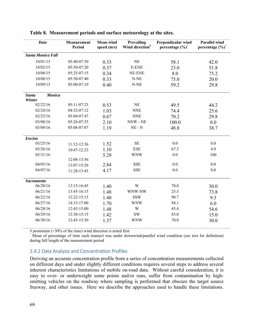
69

Table 8. Measurement periods and surface meteorology at the sites.

Date Measurement Period

Mean wind speed (m/s)

Prevailing Wind direction#

Perpendicular wind percentage (%)^

Parallel wind percentage (%)^

Santa Monica Fall

10/01/15 05:40-07:30 0.33 NE 58.1 42.0 10/02/15 05:50-07:20 0.37 E-ENE 23.0 51.8 10/06/15 05:25-07:15 0.34 NE-ENE 8.0 75.2 10/08/15 05:50-07:40 0.33 N-NE 75.0 20.0 10/09/15 05:00-07:10 0.40 N-NE 59.2 29.8

Santa Monica Winter

02/22/16 05:11-07:25 0.53 NE 49.5 44.2 02/24/16 04:52-07:12 1.03 NNE 74.4 25.6 02/25/16 05:04-07:47 0.67 NNE 70.2 29.8 03/08/16 05:26-07:35 2.10 NNW - NE 100.0 0.0 03/09/16 05:08-07:07 1.19 NE - N 48.8 38.7

Encino

03/25/16 11:12-12:36 1.52 SE 0.0 0.0 03/26/16 10:47-12:23 1.10 ESE 67.3 4.9 03/31/16

12:08-13:56 5.29 WNW 0.0

100

04/05/16 13:07-15:26 2.84 SSE 0.0 0.0 04/07/16 11:28-13:43 4.17 SSE 0.0 0.0

Sacramento

06/20/16 13:15-16:45 1.40 W 70.0 30.0 06/21/16 13:45-16:15 1.48 WNW-NW 25.5 73.8 06/22/16 12:22-15:15 1.40 SSW 90.7 9.3 06/27/16 14:15-17:00 1.70 WNW 94.1 6.0 06/28/16 12:45-15:00 1.48 W 45.4 54.6 06/29/16 12:30-15:15 1.42 SW 83.0 15.0 06/30/16 12:45-15:30 1.37 WNW 70.0 30.0

# prominent (>30% of the time) wind direction is noted first ^ Mean of percentage of time each transect was under downwind/parallel wind condition (see text for definition) during full length of the measurement period

2.4.2 Data Analysis and Concentration Profiles 

Deriving an accurate concentration profile from a series of concentration measurements collected on different days and under slightly different conditions requires several steps to address several inherent characteristics limitations of mobile on-road data. Without careful consideration, it is easy to over- or underweight some points and/or runs, suffer from contamination by high-emitting vehicles on the roadway where sampling is performed that obscure the target source freeway, and other issues. Here we describe the approaches used to handle these limitations.

70

Many of the approaches used here were carefully developed in Ranasinghe et al. (2016) and Choi et al. (2013).

First, data sets from different instruments on the MMP were synchronized, accounting for the different response times of instruments. A time-lag correlation method, described in detail in Choi et al. (2012a), was used for the calculation of the instrument response times and data synchronization. Then the contribution from high-emitting vehicles (HEV) encountered along the sampling route was removed from the concentration time series. HEV data have a strong stochastic element and a potential to obscure general trends in concentration variations. For this analysis, we are interested in the decay trend of the freeway plume. HEV encounters along the transect are not of interest and thus are removed. The method developed by Choi et al. (2013) was modified to identify HEV-related spikes. This method uses an iterative statistical approach to establish a site- and session-specific baseline threshold (BT) to determine events caused by HEVs. For all sites, the BT was calculated for a 60 s smoothing time window. At proximity to the freeway it is hard to distinguish the freeway plume and the local traffic emissions. Therefore, in this study, the threshold value was gradually increased for distance bins closer to the freeway and at very close to the freeway all data points were retained. This method successfully removed the narrow HEV-related spikes from the concentration time series, while retaining the wide freeway-related spikes.

Site specific distance bins were chosen based on the location of local roads and general traffic volume on those roads during the measurement period. At all sites, at very close to the freeway the local roads were very low trafficked, resulting in minimal effects from HEV related spikes. At the Santa Monica, all data points at a distance less than 40 m from the edge of the freeway were retained. For 40-150 m distance bin the threshold was 12×BT, for 150-300 m distance bin the threshold was 9BT, for 300-450 m distance bin the threshold was 6BT and at all distances larger than 450 m the threshold was 3BT. At the Sacramento site, all data points at a distance less than 40 m from the edge of the freeway were retained. For 40-75 m distance bin the threshold was 24BT, for 75-120 m distance bin the threshold was 12BT, for 120-160 m distance bin the threshold was 6BT and at all distances larger than 160 m the threshold was 3BT. All concentration values above the calculated threshold were replaced by the baseline concentration values to obtain the HEV spike-removed concentration time series. At distances less than 40 m from the edge of the freeway, any short-lived HEV related spikes observed were manually removed with the use traffic video from the MMP. The HEV removal calculations were repeated with several small increments and decrements to the distance bins and threshold values to investigate the sensitivity of the final results to the values chosen in the HEV removal process. No observable change was shown in the results, indicating a low sensitivity.

The effect of barriers on pollution dispersion downwind has shown to be heavily dependent on the wind direction (Finn et al., 2010, Steffens et al., 2012). We used the metrological data collected at an upwind location to partition all concentration data according to wind direction. The concentration data was sectioned in to near-perpendicular downwind data sets and a near-parallel data sets. Near perpendicular/downwind was defined as when the wind direction was ± 450 from perpendicular to the freeway. Parallel/near-parallel was defined as when the wind direction was ±450 from the parallel to the freeway. After partitioning by the wind direction, all the concentration data sets were normalized by the freeway traffic flow at each site. The traffic flow calculations are described in section 2.2.1. As the concentration measurement at a

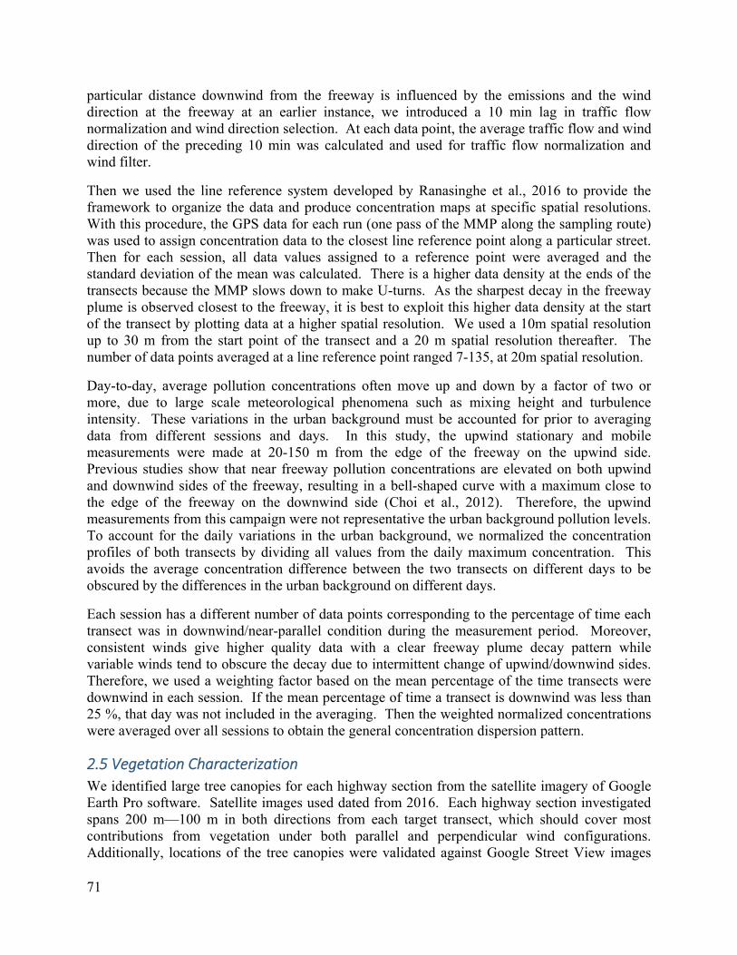
71

particular distance downwind from the freeway is influenced by the emissions and the wind direction at the freeway at an earlier instance, we introduced a 10 min lag in traffic flow normalization and wind direction selection. At each data point, the average traffic flow and wind direction of the preceding 10 min was calculated and used for traffic flow normalization and wind filter.

Then we used the line reference system developed by Ranasinghe et al., 2016 to provide the framework to organize the data and produce concentration maps at specific spatial resolutions. With this procedure, the GPS data for each run (one pass of the MMP along the sampling route) was used to assign concentration data to the closest line reference point along a particular street. Then for each session, all data values assigned to a reference point were averaged and the standard deviation of the mean was calculated. There is a higher data density at the ends of the transects because the MMP slows down to make U-turns. As the sharpest decay in the freeway plume is observed closest to the freeway, it is best to exploit this higher data density at the start of the transect by plotting data at a higher spatial resolution. We used a 10m spatial resolution up to 30 m from the start point of the transect and a 20 m spatial resolution thereafter. The number of data points averaged at a line reference point ranged 7-135, at 20m spatial resolution.

Day-to-day, average pollution concentrations often move up and down by a factor of two or more, due to large scale meteorological phenomena such as mixing height and turbulence intensity. These variations in the urban background must be accounted for prior to averaging data from different sessions and days. In this study, the upwind stationary and mobile measurements were made at 20-150 m from the edge of the freeway on the upwind side. Previous studies show that near freeway pollution concentrations are elevated on both upwind and downwind sides of the freeway, resulting in a bell-shaped curve with a maximum close to the edge of the freeway on the downwind side (Choi et al., 2012). Therefore, the upwind measurements from this campaign were not representative the urban background pollution levels. To account for the daily variations in the urban background, we normalized the concentration profiles of both transects by dividing all values from the daily maximum concentration. This avoids the average concentration difference between the two transects on different days to be obscured by the differences in the urban background on different days.

Each session has a different number of data points corresponding to the percentage of time each transect was in downwind/near-parallel condition during the measurement period. Moreover, consistent winds give higher quality data with a clear freeway plume decay pattern while variable winds tend to obscure the decay due to intermittent change of upwind/downwind sides. Therefore, we used a weighting factor based on the mean percentage of the time transects were downwind in each session. If the mean percentage of time a transect is downwind was less than 25 %, that day was not included in the averaging. Then the weighted normalized concentrations were averaged over all sessions to obtain the general concentration dispersion pattern.

2.5 Vegetation Characterization 

We identified large tree canopies for each highway section from the satellite imagery of Google Earth Pro software. Satellite images used dated from 2016. Each highway section investigated spans 200 m—100 m in both directions from each target transect, which should cover most contributions from vegetation under both parallel and perpendicular wind configurations. Additionally, locations of the tree canopies were validated against Google Street View images

72

seen from the highways and from the local roads. For the two sites in the Los Angeles region (Santa Monica and Encino), the identified tree locations were additionally validated in field visits. We did not find any significant misrepresentation of tree objects in Google Earth Pro compared with field observations, indicating the reliability of the geolocational data in Google Earth Pro.

Horizontal dimensions of the trees and their heights with respect to the highway road surface, and distances to the local road section where air sampling were conducted, were measured in Google Earth Pro. We validated the tree heights at the I-10 sections using trigonometric methods in the field and found that measurements from Google Earth Pro were within 10% accuracy compared with field values.

Optical porosity (also known as foliage transparency in forestry) of the tree crowns were measured according to a field guide for vegetation structure measurements by the US Forest Service (USFS, 2011). The tree crown as seen by the observer is compared with the images of tree crowns with known density values on a standard Crown Density–Foliage Transparency Card to determine the optical porosity. Measurements of the optical porosity values of the canopies in I-10 and 101 sections were conducted in the field near the highway soundwalls using this USFS method (USFS 2011). For canopies in CA-99 sections, we extracted screenshots from the Google Street View at the exact locations on the highway and estimated the optical porosity with the same method. For CA-99 sections, the Google Street View images were shot in August 2016, which is close to the time when we did air sampling.

Average optical porosity for each section was calculated by weighting optical porosity of individual canopy by length along the highway direction, and height. Gaps between tree canopies were also accounted for by assigning 100% porosity. We followed these steps in calculating the average optical porosity:

1. Calculate the average height of the trees weighted by their widths. If the height of the tree is , the width is , and the total length of canopy-covered section is ∗ (excluding gap

segments), then the average height is

∑∗

Note that gaps between trees are not considered in the above equation.

2. Calculate the height-weighted average crown density using the average tree height as the threshold. For overlapping trees, crown density ( ) in the overlapping are cannot exceed one. The reason to use crown density (1 – optical porosity) for the averaging instead of optical porosity is that, the sky portion above a tree canopy will be automatically accounted as having zero density this way. The average crown density of the section is

∑ ⋅

where is the total length of the section including canopies and gaps (200 m).

73

3. The average optical porosity is then the reverse of the average crown density on a 0 to 1 scale, i.e.,

1

The average heights and porosities for each location are listed in Table 10 in the results section. Photographs and porosity for each tree are also shown in the results.

 

3. Results and Discussion Several types of measurement approaches as well as data analyses were performed to probe the differences between different barrier configurations, including stationary measurements. The results and discussion are organized primarily by site (Santa Monica, Sacramento, Encino and Riverside). Additional sections describe model development and analyses performed on subsets of the data to address focused questions and look in more detail to parts of the data, including a discussion of the role of particle losses on leaves. The results for main sites (those with vegetation; Santa Monica, Encino and Sacramento) are presented as follows: a) a description of the vegetation, b) a summary of the profiles derived from mobile results, including decay profiles during both “perpendicular” and “parallel” wind conditions, and c) a summary of the continuous fixed-site results. For all analyses, wind within ± 45º of perpendicular to the freeway was classified as perpendicular, and wind within ± 45º of the freeway was classified as parallel.

3.1 Optical Porosity of Vegetation at the Santa Monica, Sacramento and Encino Sites 

Optical porosity of vegetation is defined as the fraction of pore spaces and gaps in the total area of the tree crown profile. Table 10 shows average heights and optical porosity for vegetation within ± 100 m of the intersection of each transect and the freeways for Santa Monica, Sacramento and Encino (the Riverside site did not have vegetation). The Table also shows the optical porosity of the comparable “scene” for the pairs of transects; this is for a height equal to the tallest tree at either transect. High porosity corresponds to low density vegetation and/or large amounts of gaps between trees. As this calculation includes a significant amount of sky, the optical porosity values calculated this way are quite high. Additionally, the inclusion of trees up to ± 100 m from the transect impacts some of the values; most freeway sections had similar quantities of trees, but the Sacramento 9th avenue site had a large block of trees beginning ~50m from one end of the transect, so for more perpendicular winds the effective optical porosity will be higher.

74

Table 9. Average height and average porosity of trees at each location on the primary downwind side, and max height of any vegetation at either of each pair of sites, and the corresponding optical porosity for the max height.

Name Mean height (m)

Mean optical porosity (dimensionless)

Max height (m)

Mean optical porosity rescaled to max height (dimensionless)

I-10/Granville Ave. (Vegetation only)

7.7 0.28 11.9 0.53

I-10/Dorchester Ave. (combination barrier)

5.9 0.57 11.9 0.79

I-101/Zelzah Ave. (Vegetation only)

7.7 0.79 24.4 0.93

I-101/Encino Ave. (combination barrier)

12.5 0.60 24.4 0.79

CA-99/9th Ave. (soundwall only; most vegetation is 50 – 100 m from the center of the transect.)

11.2 0.75 20.1 0.86

CA-99/19th Ave. (combination barrier)

14.6 0.49 20.1 0.63

75

Figure 37. Effective optical porosity as a function of height. The solid lines indicate the heights up to the maximum height of any tree in the scene; dotted lines include increasing amounts of clear sky. High porosity corresponds to low tree density and/or gaps between trees.

In general, it is very difficult to link optical porosity directly with tree species, since the leaf area of a tree species is not a consistent parameter, but depends on the tree stand age and environmental parameters such as water stress, nutrient status, etc. With this significant caveat in mind, Table 11 shows a very qualitative description of the optical porosity of several species identifiable at the Santa Monica and Encino sites.

76

Table 10. Very approximate optical porosity for some representative tree species observed

at the study sites in Southern California

Tree species Optical porosity*

Schinus molle high

Schinus terebinthifolius high

Chilopsis linearis high

Jacaranda mimosifolia medium

Afrocarpus falcatus medium

Pinus canariensis high

Eucalyptus polyanthemos medium

Cupressus sempervirens low

Fraxinus uhdei medium *High (> 60%), medium (30–60%), low (< 30%). The lower the optical porosity, the denser the tree crown.

3.2  I‐10  Santa  Monica  Profiles,  Continuous  Fixed‐Site  Results  and  Vegetation Characterization 

3.2.1 Vegetation Characterization 

Figure 38 and Figure 39 show birds eye view images of the Santa Monica transects, with specific trees or groups of trees labelled and corresponding to optical porosity estimates shown in Figure 40. The vegetation at Granville Ave. (Figure 38 and Figure 40; no soundwall) is considerably denser and somewhat taller than the vegetation at Dorchester (Figure 39 and Figure 40; with soundwall).

77

Figure 38. Aerial view and locations of trees labelled in Figure 40 at the Granville transect in Santa Monica.

Figure 39. Aerial view and locations of trees labelled in Figure 40 at the Granville transect in Santa Monica.

Table 11 shows most of the tree species at the Santa Monica site. Except for several cypress trees at Granville Ave. and a pine at Dorchester Ave., all species are broadleaf trees that do not drop their leaves in winter.

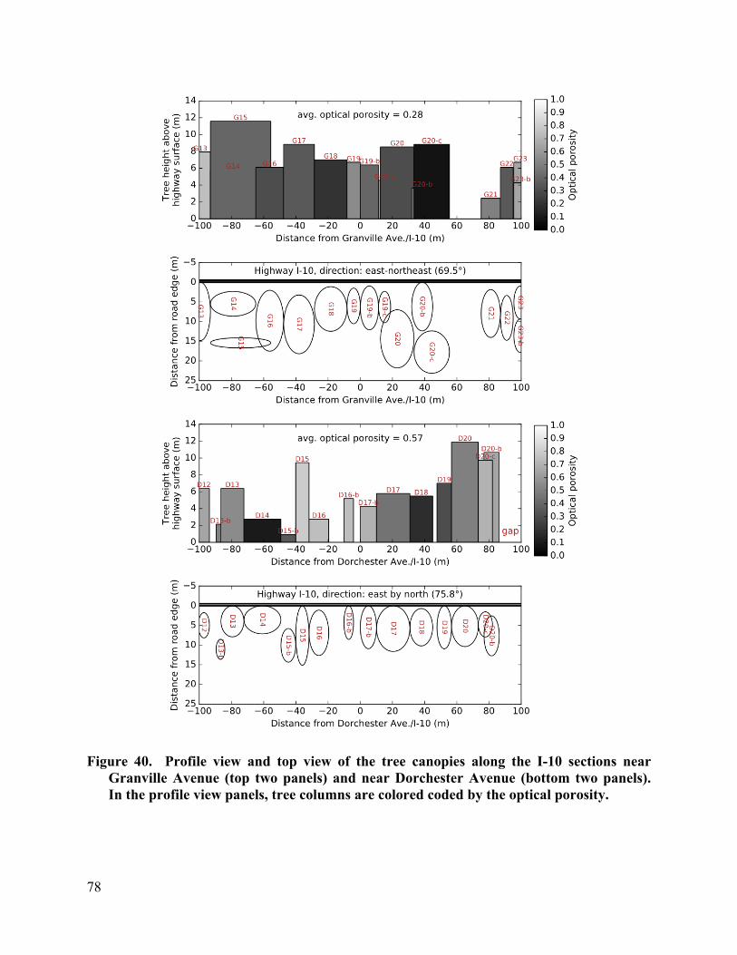
78

Figure 40. Profile view and top view of the tree canopies along the I-10 sections near Granville Avenue (top two panels) and near Dorchester Avenue (bottom two panels). In the profile view panels, tree columns are colored coded by the optical porosity.

79

Table 11. Tree species observed at the Santa Monica transects

Dorchester Ave.  Granville Ave. Schinus molle Cupressus sempervirens (several) Morus Alba Schinus terebinthifolius (several) Ulmus parvifolia Jacaranda mimosifolia (several) Chilopsis linearis Fraxinus uhdei Jacaranda mimosifolia Afrocarpus falcatus Pinus canariensis Eucalyptus polyanthemos

3.2.2 Decay Profiles from Mobile and Passive Measurements 

Figure 41 shows the background and traffic normalized [UFP] at the Santa Monica site, under downwind conditions, averaged over all wind speeds and all the days of a session. In both sessions, the measurements were made in the early morning hours close to sunrise (Table ). The [UFP] shows a gradual decay up to about 500 m, in both sessions. This agrees with earlier studies that found in pre-sunrise hours, with stable, nocturnal meteorological conditions, the freeway plume can be elongated up to 2 km (Hu et al, 2009, Choi et al., 2012).

At the Santa Monica site, the [UFP] reduction behind the barriers showed different trends over the two measurement sessions. In the fall session, the vegetation-only barrier showed a higher [UFP] reduction than the combination barrier (Figure 41 (a)), while in the winter session, the combination barrier showed a higher reduction than the vegetation-only barrier (Figure 41 (b)). The surface meteorology in the two sessions was different in several aspects and that could have contributed the observed differences in pollution plume decay downwind of the freeway. The average wind speed in the fall session was 0.4 ± 0.1 m/s, while in winter session it was 1.1 ± 0.4 m/s (an investigation of the wind speed dependence of the pollution reduction is presented below). The wind direction was more variable in fall session than winter session. The average percentage of time transects were downwind (as defined above) of the freeway was 44.7 ± 28.0 % in the fall session and 68.6 ± 21.1 % in the winter session. In the fall sessions, this resulted in a lower number of measurement days with sufficient downwind data to plot the concentration decay. Moreover, under variable wind directions, due to the intermittent change of upwind/downwind sides of the freeway, the upwind pollution levels tend to increase and downwind pollutions levels tends to decrease, affecting the downwind concentration decay pattern.

80

Figure 41. The variation of normalized UFP number concentration along the two transects at the I-10 Santa Monica site under downwind conditions for (a) Fall 2015 and (b) Winter 2016 measurement sessions. The background and traffic normalized concentration averaged over (a) 3 (b) 5 sessions (color points) is plotted together with the standard error of the mean (black whiskers).

At the Santa Monica site, in the fall season, under downwind conditions, averaged over all days (all days had wind speeds less than 0.6 m/s) and along the total length of the transects, the [UFP] concentration reduction behind the combination barrier was 50.7% lower compared to the vegetation-only barrier. In the first 160 m (~ 525 ft.) from the edge of the freeway, this difference was 40.5 %. In the winter session, under downwind conditions, averaged over days with wind speed higher than 0.6 m/s and along the total length of the transects, the [UFP] concentration reduction behind both the combination barrier and the vegetation-only barrier is approximately equal. But in the first 160 m from the edge of the freeway, [UFP] concentration

(a)

(b)

81

reduction behind the combination barrier was 25.1% lower compared to the vegetation-only barrier.

Figure 42 shows the background and traffic normalized [UFP] at the Santa Monica site, under parallel wind condition, averaged over all wind speeds and all the days of a session. In both sessions, a higher reduction was observed behind the combination barrier at the start of the transects. In fall, averaged over the first 80 m from the edge of the freeway, this additional reduction was 19 %. In winter, averaged over the first 60 m from the edge of the freeway, the additional reduction was 6.6 %.

Figure 42. The variation of normalized UFP number concentration along the two transects at the I-10 Santa Monica site, under parallel wind conditions for (a) Fall 2015 and (b) Winter 2016 measurement sessions. The background and traffic normalized concentration averaged over 4 sessions (color points) is plotted together with the standard error of the mean (black whiskers).

(a)

(b)

82

3.2.3 Continuous Measurements from Passive Samplers: NO and NO2 Profiles  

Figure 43, Figure 44 and Figure 45 show NO and NO2 concentrations vs. distance data collected with passive NOx samplers during three field campaigns in Santa Monica. Figure 46 shows a wind rose for the first campaign (May-June 2015), and Table 12 shows the data in tabular form. During that campaign the wind direction was perpendicular (165° or 345°, ± 45°) to the orientation of the freeway (i.e., ~75°) only for ~43% of the sampling period; whereas, the remaining ~57% was parallel (75° or 255°, ± 45°) to the freeway in Santa Monica. At this study site, the wind intensity was also particularly low (~ 0.79 m/s, averaged over the entire period).

The Santa Monica site was chosen to study calm atmospheric conditions which in the mornings when pollutant concentrations can be very high, but also at night when emissions are low. However, for most the day, the target area is upwind of the freeway and intersects some busy surface streets. While there is a pronounced plume from the freeway in the morning (see Section 3.2.2), profiles are indistinct over 24 hours, and there is no significant difference between the two barrier configurations, a result that was reproduced in all three field campaigns.

Figure 43. NO and NO2 concentration data collected from Ogawa passive samplers distributed near I-10 in Santa Monica during May-June 2015 along (a) Dorchester Ave. (vegetation and soundwall); and, (b) Granville Ave. (vegetation only).

83

Figure 44. NO and NO2 concentration data collected from Ogawa passive samplers distributed near I-10 in Santa Monica during Sept.-Oct. 2015 along (a) Dorchester Ave. (vegetation and soundwall); and, (b) Granville Ave. (vegetation only).

Figure 45. NO and NO2 concentration data collected from Ogawa passive samplers distributed near I-10 in Santa Monica during Feb. - March 2016 along (a) Dorchester Ave. (vegetation and soundwall); and, (b) Granville Ave. (vegetation only).

84

Figure 46. Wind rose for data in Figure 43. The gray arrow indicates the orientation of I-10.

Table 12. A summary of NO and NO2 data in tabular form for the data in Figure 43 along the I-10 freeway in Santa Monica, CA.

Vegetation and Soundwall Vegetation Only Distance

(m) NOx

(ppb) NO2

(ppb) NO

(ppb)Distance

(m)NOx

(ppb) NO2

(ppb) NO

(ppb)

-800 14.89 6.08 8.81 -800 14.89 6.08 8.81-15 18.31 9.00 9.31 -15 18.31 9.00 9.3115 11.35 5.47 5.87 15 12.54 6.08 6.4670 11.62 5.18 6.44 70 9.87 5.11 4.76

200 11.87 5.77 6.10 200 10.41 5.14 5.27

400 10.12 4.51 5.62 400 10.88 5.11 5.77

3.2.4 Continuous Paired‐Site Measurements of UFP, PM2.5, and BC 

Figure 47 shows an overview of particle size distributions at upwind and downwind locations of two study sites: (a) vegetation barrier and (b) combination barrier at the I-10 study site in Santa Monica. The solid black lines represent the median of size-resolved particle concentration data

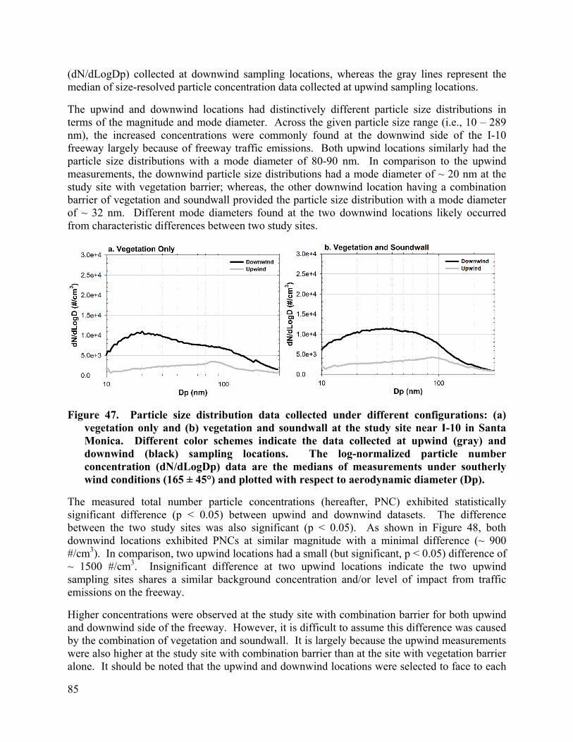
85

(dN/dLogDp) collected at downwind sampling locations, whereas the gray lines represent the median of size-resolved particle concentration data collected at upwind sampling locations.

The upwind and downwind locations had distinctively different particle size distributions in terms of the magnitude and mode diameter. Across the given particle size range (i.e., 10 – 289 nm), the increased concentrations were commonly found at the downwind side of the I-10 freeway largely because of freeway traffic emissions. Both upwind locations similarly had the particle size distributions with a mode diameter of 80-90 nm. In comparison to the upwind measurements, the downwind particle size distributions had a mode diameter of ~ 20 nm at the study site with vegetation barrier; whereas, the other downwind location having a combination barrier of vegetation and soundwall provided the particle size distribution with a mode diameter of ~ 32 nm. Different mode diameters found at the two downwind locations likely occurred from characteristic differences between two study sites.

Figure 47. Particle size distribution data collected under different configurations: (a) vegetation only and (b) vegetation and soundwall at the study site near I-10 in Santa Monica. Different color schemes indicate the data collected at upwind (gray) and downwind (black) sampling locations. The log-normalized particle number concentration (dN/dLogDp) data are the medians of measurements under southerly wind conditions (165 ± 45°) and plotted with respect to aerodynamic diameter (Dp).

The measured total number particle concentrations (hereafter, PNC) exhibited statistically significant difference (p < 0.05) between upwind and downwind datasets. The difference between the two study sites was also significant (p < 0.05). As shown in Figure 48, both downwind locations exhibited PNCs at similar magnitude with a minimal difference (~ 900 #/cm3). In comparison, two upwind locations had a small (but significant, p < 0.05) difference of ~ 1500 #/cm3. Insignificant difference at two upwind locations indicate the two upwind sampling sites shares a similar background concentration and/or level of impact from traffic emissions on the freeway.

Higher concentrations were observed at the study site with combination barrier for both upwind and downwind side of the freeway. However, it is difficult to assume this difference was caused by the combination of vegetation and soundwall. It is largely because the upwind measurements were also higher at the study site with combination barrier than at the site with vegetation barrier alone. It should be noted that the upwind and downwind locations were selected to face to each

86

other across the I-10 freeway (as seen in figure 11). Therefore, it is possible that the background difference measured at the upwind sampling locations (~ 900 #/cm3) could also cause the similar level of difference (~ 1500 #/cm3) at the downwind measurements, in addition to any effects of vegetation or soundwall.

Figure 48. Total number particle concentrations for: vegetation only (left) and vegetation with soundwall (right) at the study site near I-10 in Santa Monica. Different color schemes indicate the data collected at upwind (dark gray) and downwind (light gray) sampling locations. The medians of the data collected under southerly wind conditions (165 ± 45°) are plotted. The error bars indicate one standard deviation.

Figure 49 shows measurements of PM2.5 and BC mass concentrations upwind and downwind of the I-10 freeway. Similar to the UFP measurements, this study observed mass concentrations of PM2.5 higher on the downwind (i.e., 8.38 µg/m3 and 11.04 µg/m3 on average at the downwind study sites with combination barrier and vegetation barrier, respectively) than the upwind (i.e., 8.05 µg/m3). Unlike the UFP data, we found the mass concentration of PM2.5 and BC were slightly higher at the area with vegetation only than at the area with vegetation and soundwall. BC mass concentration showed 1.51 µg/m3 with vegetation only and 1.18 µg/m3 with combination of vegetation and soundwall. The observed differences were small but statistically significant (p < 0.05). See Table 14 for a summary of measurements at the I-10 study site in Santa Monica.

87

Figure 49. (a) PM2.5 and (b) black carbon (BC) data collected under different configurations: vegetation only (left) and vegetation with soundwall (right) at the study site near I-10 in Santa Monica. Different color schemes indicate the data collected at upwind (dark gray) and downwind (light gray) sampling locations. The medians of the data collected under northerly wind conditions (345 ± 45°) are plotted. The error bars indicate one standard deviation of the measurements.

Table 13. A summary of UFP, PM2.5, BC concentration measurements at the upwind and downwind sampling locations of vegetation only (VO) and vegetation with soundwall (VW) sites along the I-10 freeway in Santa Monica, CA.

I-10 Santa Monica, CA UFP (#/cm3) PM2.5 (μg/m3) BC (µg/m3)

Upw

ind

VO

Median 3206.69 6.45 NA

St.Dev. 1991.91 5.80 NA

Mean 3846.14 8.05 NA

VW

Median 4738.80 NA NA

St.Dev. 3880.83 NA NA

Mean 3846.14 NA NA

Dow

nwin

d VO

Median 12966.40 9.05 1.42

St.Dev. 11103.76 6.76 0.99

Mean 14857.22 11.04 1.51

VW

Median 13802.50 5.89 1.16

St.Dev. 10717.62 6.08 1.17

Mean 15020.48 8.38 1.18

 

 

88

3.2.5 Difference‐in‐Differences 

To understand the effect of vegetation added to a soundwall barrier, we first evaluate the differences between upwind and downwind pollutant concentrations at each study site (e.g., the left panel of Figure 50, comparing dVW and dVO). Then, the following DID analysis determined DID value (e.g., the right panel of Figure 51, DID = dVO – dVW).

The left panels of Figures 50 and 51 show small (but statistically significant, p < 0.05) differences in UFP, PM2.5, and BC concentrations between the study site with vegetation only and the other study site with combination barrier near the I-10 in Santa Monica. As shown in Figure 50, the downwind-upwind difference in the area with combination barrier (i.e., dVW) was slightly higher than in the area with vegetation only (dVO). The median of upwind-subtracted PNC was 6344 (± 6279) #/cm3 in the area with vegetation only but increased to 8372 (± 10787) #/cm3 in the area with combination barrier.

The difference-in-differences (difference between dVO and dVW or, DID = dVO – dVW) in Santa Monica is small but the difference is statistically significant (p < 0.05). Accordingly, the difference-in-differences becomes a negative value: – 903 (± 14243) #/cm3. Under the given method for DID analysis, the negative DID values could be interpreted as an overall increase of UFP when adding a soundwall barrier in the vegetated area near the I-10 in Santa Monica. However, it should be noted that the difference is small and variability of DID estimates is high. Similar observations were repeated in the following DID analysis with the PM2.5 data from this sampling site (see figure 51).

Figure 50. Downwind-upwind differences and Difference-in-Differences (DID) for total number particle concentrations for vegetation only (dVO, black) and vegetation and soundwall (dVW, gray) near the I-10 in Santa Monica, CA. The dark gray bar indicates the DID value (i.e., DID = dVO – dVW). Medians with one standard deviation are shown.

89

Negative DID values were observed again in PM2.5 measurements from the sampling campaign in Santa Monica. Figure 51 presents the differences (i.e., dVO and dVW) and DID values for PM2.5 and BC. For PM2.5, the estimated dVO and dVW, were – 0.37 (± 1.47) μg/m3 and -0.11 (± 1.65) μg/m3, respectively. Similar to UFP data, this study found a significant difference (p < 0.05) between dVO and dVW for PM2.5. The complex nature of this near-freeway data collection resulted in a high variability in the downwind-upwind differences (dVO and dVW), which can provide a negative DID values for either barrier configurations. However, the difference in PM2.5 measurements is small and remains within the error range (< 1.00 μg/m3) of the instrument (TSI Inc., Shoreview, MN Model 8520). Unlike UFP and PM2.5 data, the BC data is 1.42 (± 0.99) μg/m3 and 1.16 (± 1.17) μg/m3 for dVO and dVW, respectively. Again, there is a significant difference (p < 0.05) between dVO and dVW of BC data. The DID value of 0.34 (± 1.17) μg/m3 indicates a little reduction of BC concentrations with additional soundwall in the existing vegetation near the I-10 in Santa Monica. Table 14 presents a summary of the difference and DID values from the data collected near the I-10 in Santa Monica.

Figure 51. Downwind-upwind differences and Difference-in-Differences (DID) for (a) PM2.5 and (b) black carbon. The differences are shown for the study areas with vegetation only (dVO, black) and with vegetation and soundwall (dVW, gray) near the I-10 in Santa Monica, CA. The dark gray bar indicates the DID value (i.e., DID = dVO – dVW). The plotted data are the medians and the error bars indicate one standard deviation.

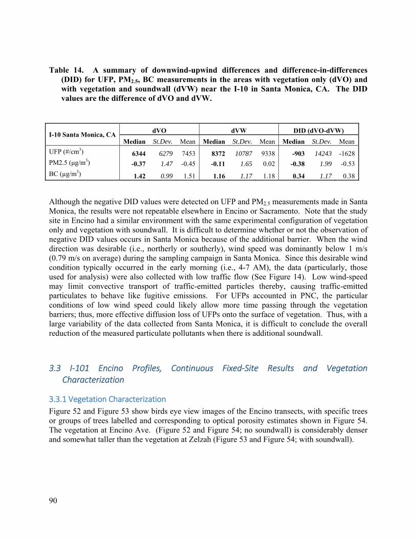
90

Table 14. A summary of downwind-upwind differences and difference-in-differences (DID) for UFP, PM2.5, BC measurements in the areas with vegetation only (dVO) and with vegetation and soundwall (dVW) near the I-10 in Santa Monica, CA. The DID values are the difference of dVO and dVW.

Although the negative DID values were detected on UFP and PM2.5 measurements made in Santa Monica, the results were not repeatable elsewhere in Encino or Sacramento. Note that the study site in Encino had a similar environment with the same experimental configuration of vegetation only and vegetation with soundwall. It is difficult to determine whether or not the observation of negative DID values occurs in Santa Monica because of the additional barrier. When the wind direction was desirable (i.e., northerly or southerly), wind speed was dominantly below 1 m/s (0.79 m/s on average) during the sampling campaign in Santa Monica. Since this desirable wind condition typically occurred in the early morning (i.e., 4-7 AM), the data (particularly, those used for analysis) were also collected with low traffic flow (See Figure 14). Low wind-speed may limit convective transport of traffic-emitted particles thereby, causing traffic-emitted particulates to behave like fugitive emissions. For UFPs accounted in PNC, the particular conditions of low wind speed could likely allow more time passing through the vegetation barriers; thus, more effective diffusion loss of UFPs onto the surface of vegetation. Thus, with a large variability of the data collected from Santa Monica, it is difficult to conclude the overall reduction of the measured particulate pollutants when there is additional soundwall.

3.3  I‐101  Encino  Profiles,  Continuous  Fixed‐Site  Results  and  Vegetation Characterization 

3.3.1 Vegetation Characterization 

Figure 52 and Figure 53 show birds eye view images of the Encino transects, with specific trees or groups of trees labelled and corresponding to optical porosity estimates shown in Figure 54. The vegetation at Encino Ave. (Figure 52 and Figure 54; no soundwall) is considerably denser and somewhat taller than the vegetation at Zelzah (Figure 53 and Figure 54; with soundwall).

I-10 Santa Monica, CA dVO dVW DID (dVO-dVW)

Median St.Dev. Mean Median St.Dev. Mean Median St.Dev. Mean

UFP (#/cm3) 6344 6279 7453 8372 10787 9338 -903 14243 -1628PM2.5 (μg/m3) -0.37 1.47 -0.45 -0.11 1.65 0.02 -0.38 1.99 -0.53

BC (µg/m3) 1.42 0.99 1.51 1.16 1.17 1.18 0.34 1.17 0.38

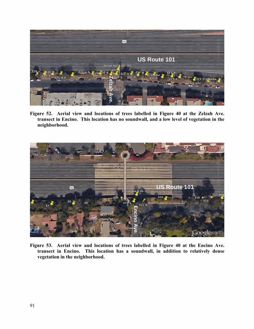
91

Figure 52. Aerial view and locations of trees labelled in Figure 40 at the Zelzah Ave. transect in Encino. This location has no soundwall, and a low level of vegetation in the neighborhood.

Figure 53. Aerial view and locations of trees labelled in Figure 40 at the Encino Ave. transect in Encino. This location has a soundwall, in addition to relatively dense vegetation in the neighborhood.

US Route 101

Zelzah

Ave.

En

cino

Ave.

US Route 101

92

Figure 54. Profile view and top view of the tree canopies along the I-101 sections near Zelzah Avenue (top two panels) and near Encino Avenue (bottom two panels). In the profile view panels, tree columns are colored coded by the optical porosity.

93

3.3.2 Decay Profiles from Mobile and Passive Monitoring 

Figure 55 shows the traffic normalized [UFP] at the Encino site, under downwind and parallel wind conditions. At this site, the wind direction was variable (Figure 58), resulting in only one day of data available under downwind conditions and parallel conditions (Table 2). Hence the plots here are not adequately representative of the general concentration decay trend at this site. Under both downwind and parallel wind conditions, the [UFP] showed lower concentrations behind the vegetation barrier in the first 70 – 90 m from the edge of the freeway and showed little or no difference and an opposite trend thereafter.

Figure 55. The variation of the normalized UFP number concentration along the two transects at the I-101 Encino site, under (a) downwind and (b) parallel wind conditions. The traffic normalized concentration of a session (color plots) is plotted together with the standard error of the mean (black).

(a)

(b)

94

3.3.3 Continuous Passive NO and NO2 Profiles 

Figure 56 shows the passive NO and NO2 data for the Encino campaign. They show a strong decay patterns as a function of distance from I-101 at the study site. Figure 57 shows the wind rose for the sampling period, and Table 15 shows the data in tabular form. The I-101 study site had northerly (0 ± 45°) and southerly (180 ± 45°) wind conditions accounting for ~47% of the sampling period. High intensity winds occurred at the I-101 site and resulted in a strong decay of NO and NO2 concentrations near the freeway. NO and NO2 concentrations decay to near background levels within 400 m on the south side of I-101, and a clear decay is also observed on the north side. The level of concentration decay is approximately 60-70% for NO and NO2 at 800 m with respect to the measurements at 15 m to the freeway. Here we observe that overall levels NO and NO2 were lower by 7-43% downwind of the combination vegetation and soundwall barrier, than at the study site with vegetation alone.

Figure 56. NO and NO2 concentration data collected from Ogawa passive samplers distributed near I-101 in Encino during Mar.-April 2016 along (a) Encino Ave. (vegetation and soundwall); and, (b) Zelzah Ave. (vegetation only).

95

Figure 57. Wind rose for March 24 -Apr 8, 2016 at Encino. The gray arrow indicates the orientation of I-101.

Table 15. NO and NO2 concentrations from Ogawa samplers deployed at Encino Mar. 24 – Apr. 8, 2016.

 

Vegetation and Soundwall Vegetation Only Distance

(m) NOx

(ppb) NO2

(ppb) NO

(ppb)Distance

(m)NOx

(ppb) NO2

(ppb) NO

(ppb)

-800 19.44 12.72 6.71 -800 19.44 12.72 6.71-15 31.12 19.12 12.00 -15 36.35 21.08 15.2715 20.17 13.07 7.10 15 29.55 17.03 12.52

100 17.27 11.50 5.77 70 21.67 13.34 8.33200 14.71 10.01 4.70 200 19.57 11.67 7.90400 15.63 9.69 5.94 400 17.26 10.39 6.87

800 13.69 8.93 4.75 800 18.19 10.82 7.38

96

3.3.4 Additional Stationary Measurements:  UFP, PM2.5, and BC 

Figure 58 shows particle size distributions at upwind and downwind locations of two study sites: (a) with vegetation barrier alone and (b) with combination barrier of vegetation and soundwall at the I-101 site in Encino, CA. The solid black lines represent the median of size-resolved particle concentration data from downwind sampling locations; whereas, the gray lines represent the median of size-resolved particle concentration data from the upwind sampling location. Due to data loss in one of four SMPS deployed, Figure 58 presents the same upwind data collected at 15 m north of the I-101 freeway in the study site with vegetation alone.

Similar to the data collected near the I-10 in Santa Monica, the upwind and downwind locations had distinctively different particle size distributions in terms of magnitude and mode diameter. In comparison to the data from the I-10 in Santa Monica, the upwind data collected near the I-101 in Encino exhibited ~ 20% increase in magnitude of PNC but decrease in mode diameter (~ 60 nm). Lower particle concentrations were observed at the downwind side of the freeway I-101 because the wind speeds were higher in Encino (i.e., 1.00 ± 0.65 m/s) than in Santa Monica (i.e., 0.79 ± 1.55 m/s). As expected, at higher wind speeds, an increased level of dilution would result in the decrease of measured concentrations in the near-freeway atmosphere. Although the downwind concentrations were lower in Encino than in Santa Monica, the observed mode diameters that were lower than that found in Santa Monica; a strong indication of freeway emissions. The mode diameters were ~ 10 nm at the downwind location with vegetation alone and at the downwind location with a combination of vegetation and soundwall.

Figure 58. Particle size distribution data collected under different configurations: (a) vegetation only and (b) vegetation and soundwall at the study site near I-101 in Encino. Different color schemes indicate the data collected at upwind (gray) and downwind (black) sampling locations. The log-normalized particle number concentration (dN/dLogDp) data are the medians of measurements under northerly wind conditions (0 ± 45°) and plotted with respect to aerodynamic diameter (Dp).

The measured total number particle concentrations showed statistically significant difference (p < 0.05) between upwind and downwind datasets (Figure 59). Figure 59 also exhibits both downwind locations had PNC in a similar magnitude but statistically significant difference (p <

97

0.05; ~ 1870 #/cm3) with higher total number particle concentrations observed from the site with vegetation alone than the site with vegetation and soundwall. The difference in the downwind measurements in the two study sites likely occurred from the effect of additional soundwall barrier. Unlike the low wind intensity (0.79 ±1.55 m/s) observed in Santa Monica, this site near the I-101 had higher wind intensity (1.00 ± 0.65 m/s) that provided a strong dominant wind. The occurrence of the desired (northerly) wind direction accompanied with high traffic flow provided the significant differences between the two study sites near the I-101 in Encino.

Figure 59. Total number particle concentration data collected under different configurations: vegetation only (left) and vegetation with soundwall (right) at the study site near I-101 in Encino. Different color schemes indicate the data collected at upwind (dark gray) and downwind (light gray) sampling locations. The medians of data collected under northerly wind conditions (0 ± 45°) are plotted. The error bars indicate one standard deviation.

In agreement with the data shown in Figure 59, mass concentrations of PM2.5 and BC (in Figure 60) were also slightly higher at the vegetation only site compared to the vegetation and soundwall site. Figure 60 presents mass concentration data for PM2.5 and BC at upwind and downwind sides of the I-101 freeway. Downwind mass concentrations of PM2.5 was higher (4.51 µg/m3) in the site with vegetation alone than in the other site with combination of vegetation and soundwall (i.e., 3.81 µg/m3); while, upwind measurement is low at 3.04 µg/m3 on average. Likewise, the downwind BC measurements were also slightly higher (0.74 µg/m3 on average) with vegetation alone than with combination barrier of vegetation and soundwall (0.53 µg/m3 on average). The observed differences were small but statistically significant (p < 0.05) between upwind and downwind PM2.5 data. The differences were also significant (p < 0.05) for downwind BC measurements from the two study sites. See Table 16 for a summary of measurements at the I-101 study site in Encino.

98

Figure 60. (a) PM2.5 and (b) black carbon (BC) data collected under different configurations: vegetation only (left) and vegetation with soundwall (right) at the study site near I-101 in Encino. Different color schemes indicate the data collected at upwind (dark gray) and downwind (light gray) sampling locations. The medians of the data collected under northerly wind conditions (0 ± 45°) are plotted. The error bars indicate one standard deviation of the measurements.

Table 16. A summary of UFP, PM2.5, BC concentration measurements at the upwind and downwind sampling locations of vegetation only (VO) and vegetation with soundwall (VW) sites along the I-101 freeway in Encino, CA.

I-101 Encino, CA UFP (#/cm3) PM2.5 (μg/m3) BC (µg/m3)

Upw

ind

VO

Median 6885.78 NA NA

St.Dev. 21490.14 NA NA

Mean 9162.66 NA NA

VW

Median 3.04 NA

St.Dev. 1.26 NA

Mean 3.37 NA

Dow

nwin

d VO

Median 10282.74 4.51 0.65

St.Dev. 6953.06 1.47 0.52

Mean 11772.25 4.58 0.74

VW

Median 8369.17 3.81 0.52

St.Dev. 12197.42 2.02 0.96

Mean 9901.66 4.20 0.53

99

3.3.5 Difference‐in‐Differences 

The study site near the I-101 in Encino provided experimental conditions similar to the study site near the I-10 in Santa Monica. This site in Encino was comparable to the site in Santa Monica in terms of vegetation density, freeway elevation, the height of soundwall, and experimental configuration of vegetation and soundwall. On the other hand, characteristic differences included higher wind speed and traffic flow. Sampling campaign in Encino had high wind speed of 1.00 m/s on average in Encino; whereas, the averaged wind speed was 0.79 m/s in Santa Monica. The data collection was also conducted with consistently high freeway traffic flow of 1221 (± 195) veh./5-min in Encino. The traffic flow in Encino was much greater than 638 ± 258 veh./5-min found during the data collection in Santa Monica.

Similar to the observations in Santa Monica, the data collected near the I-101 in Encino exhibited the effects of additional reduction in UFPs, PM2.5, and BC concentrations when there is a soundwall barrier in the existing vegetation. The differences of UFP, PM2.5, and BC concentrations between the area with vegetation only and the area with combination barrier of vegetation and soundwall were small, but statistically significant (p < 0.05). As shown in Figure 61, the downwind-upwind difference in the area with both vegetation and soundwall was lower than with vegetation alone. The median of upwind-subtracted PNC was 3145 (± 23530) #/cm3 in the area with vegetation only but decreased to 1761 (± 25614) #/cm3 in the area with vegetation and soundwall. This indicates the combination barrier was more effective for reducing particles downwind than vegetation alone. The difference-in-differences (i.e., DID = dVO – dVW) was determined to be 1806 (± 7418) #/cm3. The estimated DID value is greater and less variable than the DID value estimated from the data collected in Santa Monica. The positive DID value indicates an overall reduction of UFP with additional soundwall at the vegetated area near the I-101 in Encino.

Figure 61. Downwind-upwind differences and Difference-in-Differences (DID) for total

number particle concentrations. The differences are shown for the study areas with vegetation only (dVO, black) and with vegetation and soundwall (dVW, gray) near the I-101 in Encino, CA. The dark gray bar indicates the DID value (i.e., DID = dVO – dVW). The plotted data are the medians and the error bars indicate one standard deviation.

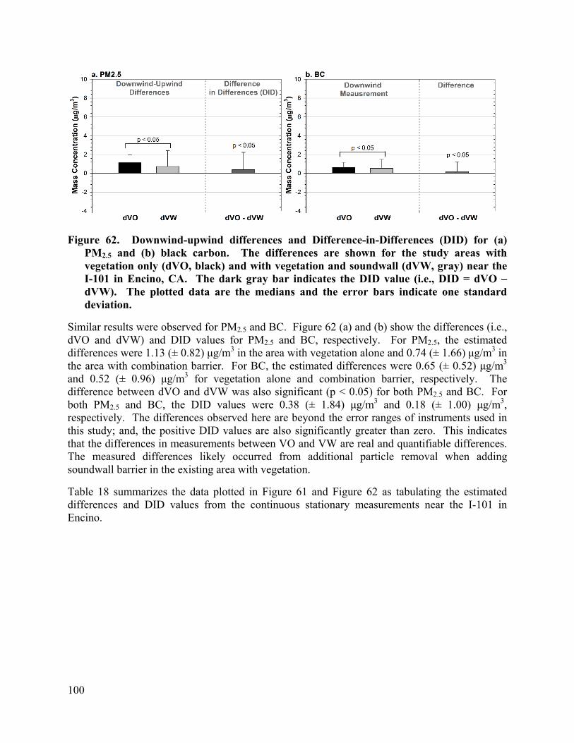
100

Figure 62. Downwind-upwind differences and Difference-in-Differences (DID) for (a) PM2.5 and (b) black carbon. The differences are shown for the study areas with vegetation only (dVO, black) and with vegetation and soundwall (dVW, gray) near the I-101 in Encino, CA. The dark gray bar indicates the DID value (i.e., DID = dVO – dVW). The plotted data are the medians and the error bars indicate one standard deviation.

Similar results were observed for PM2.5 and BC. Figure 62 (a) and (b) show the differences (i.e., dVO and dVW) and DID values for PM2.5 and BC, respectively. For PM2.5, the estimated differences were 1.13 (± 0.82) μg/m3 in the area with vegetation alone and 0.74 (± 1.66) μg/m3 in the area with combination barrier. For BC, the estimated differences were 0.65 (± 0.52) μg/m3 and 0.52 (± 0.96) μg/m3 for vegetation alone and combination barrier, respectively. The difference between dVO and dVW was also significant (p < 0.05) for both PM2.5 and BC. For both PM2.5 and BC, the DID values were 0.38 (± 1.84) μg/m3 and 0.18 (± 1.00) μg/m3, respectively. The differences observed here are beyond the error ranges of instruments used in this study; and, the positive DID values are also significantly greater than zero. This indicates that the differences in measurements between VO and VW are real and quantifiable differences. The measured differences likely occurred from additional particle removal when adding soundwall barrier in the existing area with vegetation.

Table 18 summarizes the data plotted in Figure 61 and Figure 62 as tabulating the estimated differences and DID values from the continuous stationary measurements near the I-101 in Encino.

101

Table 17. A summary of downwind-upwind differences and difference-in-differences (DID) for UFP, PM2.5, BC measurements in the areas with vegetation only (dVO) and with vegetation and soundwall (dVW) near the I-101 in Encino, CA. The DID values are the difference of dVO and dVW.

3.3.5.1 Discussion of Encino and Santa Monica Results 

The effectiveness of an additional soundwall barrier appeared to depend on wind speed and vegetation. The two sampling campaigns in Santa Monica and Encino offered measurement data collected under the same experimental configuration (i.e., vegetation only vs. vegetation and soundwall). However, the small but significant increase in UFPs and PM2.5 when “adding” a soundwall was observed at low averaged wind speed of 0.79 m/s in Santa Monica; whereas, the opposite results – overall reductions occurred in the similar environment with higher wind speed averaged at 1.00 m/s.

Even at small increments, increased wind speed could provide sufficient momentum for convective transport of traffic-emitted particles. Accordingly, traffic-emitted airborne particulates could reach over the soundwall barrier in Encino. As seen in Figure 60, the downwind PM2.5 concentrations were significantly higher than the upwind under high averaged wind speed (1.00 m/s) in Encino. On the other hand, low averaged wind speed of 0.79 m/s in Santa Monica resulted comparable PM2.5 concentrations upwind (i.e., background) and downwind of the I-10 freeway, as seen in Figure 51 (a).

Tabulated in Table 16, the estimated DID values overall indicate a little effect of particle increase or reduction with an additional soundwall in vegetated areas. It is also difficult to compare across study sites because each had different levels of traffic flow (i.e., traffic emissions) in addition to wind speed. However, with respect to the measurements in the area of vegetation alone, an additional soundwall barrier resulted in a 6.9% increase of PNC and 4.7% increase of PM2.5 at low averaged wind speed of 0.79 m/s in Santa Monica. In comparison, at slightly higher averaged wind speed of 1.00 m/s in Encino, a 17.5% reduction of PNC (i.e., UFP number concentration) and 11.2% reduction of PM2.5 mass concentration was observed. Similarly, the overall reduction of BC was 23.9% at 0.79 m/s in Santa Monica and 27.7% at 1.00 m/s in Encino.

In summary, the small change of wind speed could increase or decrease effectiveness of an additional soundwall barrier in the vegetated area.

I-101 Encino, CA

dVO dVW DID (dVO-dVW) Median St.Dev. Mean

Median St.Dev. Mean

Median St.Dev. Mean

UFP (#/cm3) 3144.9

2 23529.8

2 2627.3

5 1761.1

6 25613.6

2 -

140.77 1805.6

1 7418.3

8 2922.9

0PM2.5 (μg/m3) 1.13 0.82 1.21 0.74 1.66 0.83 0.38 1.84 0.38

BC (µg/m3) 0.65 0.52 0.74 0.52 0.96 0.53 0.18 1.00 0.21

102

3.4  Sacramento  CA‐99  Profiles,  Continuous  Fixed‐Site  Results  and  Vegetation Characterization 

3.4.1 Vegetation Characterization 

Figure 63 and Figure 64 show birds eye photographs of the Sacramento transects, with specific trees or groups of trees labelled and corresponding to optical porosity estimates shown in Figure 65. In the immediate vicinity of 9th Avenue there is minimal vegetation, consisting of a few isolated individual tall (~12 m) trees (Figure 63, and Figure 65). As we included in the analysis ± 100 m of the target transect, the scene does show some dense trees, beginning 50 m from the center of the transect. The 9th Avenue site has soundwall only with minimal vegetation, whereas the 19th Avenue has both vegetation and soundwall. The trees at the 19th St. site were a mixture of Honey Locust (Gleditsia triacanthos) and Australian Pine (Casuarina equisetifolia).

Figure 63. Google Earth photograph of CA-99 near the intersection with 9th Ave. in Sacramento, and adjacent streets. Yellow pins and accompanying white numbers indicate specific trees or groups of trees labelled in Figure 65.

CA

-99 9th Ave.

103

Figure 64. Google Earth photograph of CA-99 near the intersection with 19th Ave. in Sacramento, and adjacent streets. Yellow pins and accompanying white numbers indicate specific trees or groups of trees labelled in Figure 65.

19th Ave.

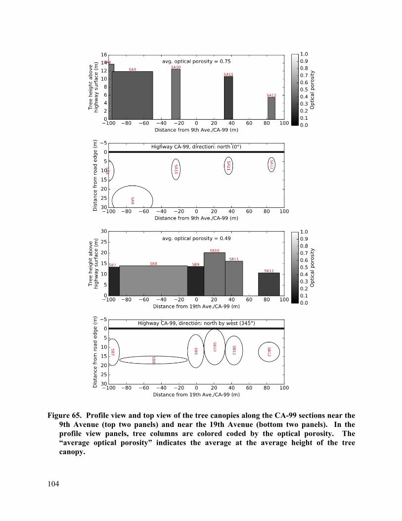
104

Figure 65. Profile view and top view of the tree canopies along the CA-99 sections near the 9th Avenue (top two panels) and near the 19th Avenue (bottom two panels). In the profile view panels, tree columns are colored coded by the optical porosity. The “average optical porosity” indicates the average at the average height of the tree canopy.

105

3.4.2 Decay Profiles from Mobile and Passive Measurements 

Figure 66 shows the background and traffic normalized [UFP] at the Sacramento site, under downwind and parallel wind conditions, averaged over all wind speeds and all measurement days. At this site, all measurements were made during daytime (Table 2). The [UFP] shows a steep decay up to about 160 m. This agrees with numerous studies that have shown that in daytime unstable meteorological conditions, the freeway plume decays rapidly and return to background concentration levels. At the Sacramento site, under downwind conditions, averaged over all wind speeds and along the total length of the transects, the [UFP] concentration behind the combination barrier was 6.3% lower relative the sound wall only transect (Figure 66a). In the first 160 m from the edge of the freeway, the reduction was larger, at this additional reduction was 15%.

Under parallel wind conditions, averaged over all wind speeds and along the total length of the transects, the [UFP] concentration reduction behind the soundwall only was 15% lower relative the combination barrier transect (Figure 66b). Concentrations are not elevated near the freeway,; indeed the profiles are nearly perfectly flat with distance from the freeway, except for the slight dip right next to the freeway at the combination site. This is consistent with a lack of influence of freeway emissions on near roadway concentrations under parallel winds. The concentrations are somewhat higher at the combination site. This may be due to differences in the urban backgrounds at the two sites due to differences in local traffic, and/or upwind sources.

The height of vegetation in combination barrier (~12 m) was higher than the soundwalls (~5 m), making the effective height of the combination barrier significantly higher than the height of the soundwall at the other transect (~ 4 m). The height of the combination barrier would result in increased vertical dispersion of the initial pollution plume. The observed lower pollution concentration behind the combination barrier site, under downwind conditions, can be attributed by this increased vertical mixing. This result agrees with a previously reported field study (Baldauf et al., 2008).

106

Figure 66. The variation of normalized UFP number concentration along the two transects at the SR-99 Sacramento site, under (a) downwind and (b) parallel wind conditions. The background and traffic normalized concentration averaged over (a) 6 (b) 4 sessions (color plots) is plotted together with the standard error of the mean (black).

Figure 67 and Figure 68 shows the traffic normalized concentration of PM2.5, BC, CO2, NO and NO2 at the Sacramento site, under downwind conditions, averaged over all wind speeds and all measurement days. The difference in pollution concentrations on the two transects was small for PM2.5, BC and CO2. On both transects, NO and NO2 concentrations decayed rapidly near the freeway. Similar to the trend shown by [UFP], concentrations behind the combination barrier were lower than that behind the soundwall.

(a)

(b)

107

Figure 67. The variation of normalized (a) PM 2.5, (b) Black Carbon and (c) CO2

concentration along the two transects at the SR-99 Sacramento site.

(a)

(b)

(c)

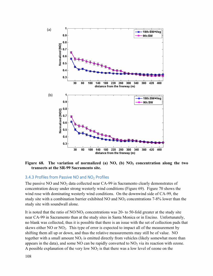
108

Figure 68. The variation of normalized (a) NO, (b) NO2 concentration along the two transects at the SR-99 Sacramento site.

3.4.3 Profiles from Passive NO and NO2 Profiles 

The passive NO and NO2 data collected near CA-99 in Sacramento clearly demonstrates of concentration decay under strong westerly wind conditions (Figure 69). Figure 70 shows the wind rose with dominating westerly wind conditions. On the downwind side of CA-99, the study site with a combination barrier exhibited NO and NO2 concentrations 7-8% lower than the study site with soundwall alone.

It is noted that the ratio of NO/NO2 concentrations was 20- to 50-fold greater at the study site near CA-99 in Sacramento than at the study sites in Santa Monica or in Encino. Unfortunately, no blank was collected, thus it is possible that there is an issue with the set of collection pads that skews either NO or NO2. This type of error is expected to impact all of the measurement by shifting them all up or down, and thus the relative measurements may still be of value. NO together with a small amount NO2 is emitted directly from vehicles (likely somewhat more than appears in the data), and some NO can be rapidly converted to NO2 via its reaction with ozone. A possible explanation of the very low NO2 is that there was a low level of ozone on the

(a)

(b)

109

sampling days, but this seems unlikely as sampling was performed in June, thus there should have been some conversion of NO to NO2.

Table 18 shows the numerical data.

Figure 69. NO and NO2 concentration data collected from Ogawa passive samplers distributed near CA-99 during June-July 2016 along (a) 19th Ave (soundwall and vegetation); and, (b) 9th Ave. (soundwall only).

Figure 70.Wind rose for the Sacramento study.

110

Table 18. Continuous passive NO and NO2 data for the Sacramento site.

3.4.4 Additional Continuous Measurements:  UFP, PM2.5, and BC 

The selected study site near the CA-99 in Sacramento had a continuous soundwall barrier with and without vegetation. Figure 71 overviews the particle size distributions data from the upwind and downwind sampling locations in two different study sites: (a) soundwall only and (b) vegetation and soundwall. The solid black lines represent the median of size-resolved particle concentration data from downwind sampling locations; whereas, the gray lines represent the median of size-resolved particle concentration data from upwind sampling locations. For comparison to downwind data, Figure 71 presents the same upwind data collected at 15 m north of the CA-99 freeway.

Similar to the data collected near the I-10 in Santa Monica and the I-101 in Encino, the upwind and downwind locations had distinctively different particle size distributions in terms of magnitude and mode diameter. The upwind data collected near the CA-99 in Sacramento exhibited greater dN/dLogDp concentration with a smaller mode diameter of ~ 50 nm compared to the I-10 and the I-101. The downwind particle concentrations were also greater than the measurements from the I-10 or the I-101. Wind speeds were higher (i.e., 1.57 ± 0.50 m/s) in Sacramento than in Encino (i.e., 1.00 ± 0.65 m/s) or in Santa Monica (i.e., 0.79 ± 1.55 m/s). Traffic flow was also higher during data collection in Encino (1221 ± 195 veh./5-min) than in Sacramento (753 ± 71 veh./5-min). Mode diameters were found near ~ 10 nm at the downwind sampling location with combination barrier and less than 10 nm at the downwind location with soundwall alone. This observation is similar to the previous observation in Encino.

Vegetation and Soundwall Soundwall Only Distance

(m) NOx

(ppb) NO2

(ppb) NO

(ppb)Distance

(m)NOx

(ppb) NO2

(ppb) NO

(ppb)

-800 6.94 0.33 6.61 -800 6.94 0.33 6.61-15 8.25 0.26 7.99 -15 10.05 0.30 9.7515 13.62 0.33 13.29 15 18.55 0.32 18.2470 11.90 0.28 11.62 50 13.22 0.24 12.98

200 12.08 0.23 11.84 100 11.41 0.27 11.14350 9.87 0.25 9.62 400 10.01 0.33 9.68

800 9.07 0.27 8.80 800 10.06 0.32 9.74

111

Figure 71. Particle size distribution data collected under different configurations: (a) soundwall only and (b) vegetation and soundwall at the study site near CA-99 in Sacramento. Different color schemes indicate the data collected at upwind (gray) and downwind (black) sampling locations. The log-normalized particle number concentration (dN/dLogDp) data are the medians of measurements under southerly wind conditions (165 ± 45°) and plotted with respect to aerodynamic diameter (Dp).

The upwind measurements were significantly lower than downwind measurements in Sacramento (p < 0.05). Similar to the previous data collected in Santa Monica and in Encino, the measured PNC showed a small but significant difference between the areas selected for soundwall only and for combination barrier in Sacrament0. The difference was also significant (p < 0.05) between the two study sites. As shown in Figure 72, both downwind locations had PNC at similar magnitude with a little difference (~ 4800 #/cm3) with PNC significantly higher at the site with soundwall alone than at the site with combination barrier (p < 0.05). The difference was likely due to the addition of vegetation.

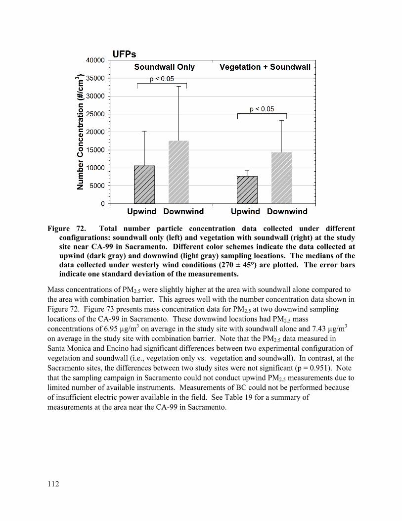
112

Figure 72. Total number particle concentration data collected under different configurations: soundwall only (left) and vegetation with soundwall (right) at the study site near CA-99 in Sacramento. Different color schemes indicate the data collected at upwind (dark gray) and downwind (light gray) sampling locations. The medians of the data collected under westerly wind conditions (270 ± 45°) are plotted. The error bars indicate one standard deviation of the measurements.

Mass concentrations of PM2.5 were slightly higher at the area with soundwall alone compared to the area with combination barrier. This agrees well with the number concentration data shown in Figure 72. Figure 73 presents mass concentration data for PM2.5 at two downwind sampling locations of the CA-99 in Sacramento. These downwind locations had PM2.5 mass concentrations of 6.95 µg/m3 on average in the study site with soundwall alone and 7.43 µg/m3 on average in the study site with combination barrier. Note that the PM2.5 data measured in Santa Monica and Encino had significant differences between two experimental configuration of vegetation and soundwall (i.e., vegetation only vs. vegetation and soundwall). In contrast, at the Sacramento sites, the differences between two study sites were not significant (p = 0.951). Note that the sampling campaign in Sacramento could not conduct upwind PM2.5 measurements due to limited number of available instruments. Measurements of BC could not be performed because of insufficient electric power available in the field. See Table 19 for a summary of measurements at the area near the CA-99 in Sacramento.

113

Figure 73. Median PM2.5 mass concentrations for soundwall only (left) and vegetation with soundwall (right) at the study site near CA-99 in Sacramento under westerly wind conditions (270 ± 45°). No data were collected at the upwind sampling locations. The error bars indicate one standard deviation.

Table 19. A summary of UFP, PM2.5, BC concentration measurements at the upwind and downwind sampling locations of soundwall only (WO) and vegetation with soundwall (VW) sites along the CA-99 freeway in Sacramento, CA

CA-99 Sacramento, CA UFP (#/cm3) PM2.5 (μg/m3) BC (µg/m3)

Upw

ind

WO

Median 10617.22 NA NA

St.Dev. 9628.06 NA NA

Mean 14544.91 NA NA

VW

Median 7682.27 NA NA

St.Dev. 1679.47 NA NA

Mean 7766.37 NA NA

Dow

nwin

d WO

Median 17643.00 4.60 NA

St.Dev. 15092.67 5.20 NA

Mean 21937.86 6.95 NA

VW

Median 14427.90 5.43 NA

St.Dev. 8822.34 4.89 NA

Mean 17136.58 7.43 NA

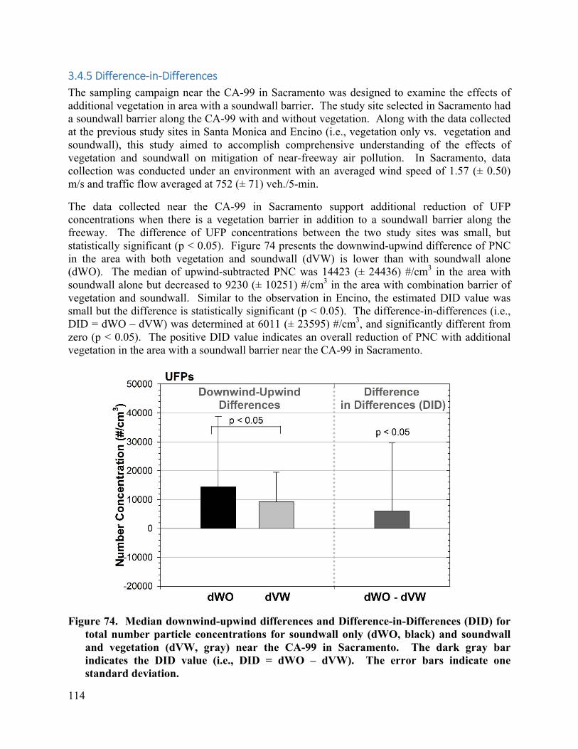
114

3.4.5 Difference‐in‐Differences 

The sampling campaign near the CA-99 in Sacramento was designed to examine the effects of additional vegetation in area with a soundwall barrier. The study site selected in Sacramento had a soundwall barrier along the CA-99 with and without vegetation. Along with the data collected at the previous study sites in Santa Monica and Encino (i.e., vegetation only vs. vegetation and soundwall), this study aimed to accomplish comprehensive understanding of the effects of vegetation and soundwall on mitigation of near-freeway air pollution. In Sacramento, data collection was conducted under an environment with an averaged wind speed of 1.57 (± 0.50) m/s and traffic flow averaged at 752 (± 71) veh./5-min.

The data collected near the CA-99 in Sacramento support additional reduction of UFP concentrations when there is a vegetation barrier in addition to a soundwall barrier along the freeway. The difference of UFP concentrations between the two study sites was small, but statistically significant (p < 0.05). Figure 74 presents the downwind-upwind difference of PNC in the area with both vegetation and soundwall (dVW) is lower than with soundwall alone (dWO). The median of upwind-subtracted PNC was 14423 (± 24436) #/cm3 in the area with soundwall alone but decreased to 9230 (± 10251) #/cm3 in the area with combination barrier of vegetation and soundwall. Similar to the observation in Encino, the estimated DID value was small but the difference is statistically significant (p < 0.05). The difference-in-differences (i.e., DID = dWO – dVW) was determined at 6011 (± 23595) #/cm3, and significantly different from zero (p < 0.05). The positive DID value indicates an overall reduction of PNC with additional vegetation in the area with a soundwall barrier near the CA-99 in Sacramento.

Figure 74. Median downwind-upwind differences and Difference-in-Differences (DID) for total number particle concentrations for soundwall only (dWO, black) and soundwall and vegetation (dVW, gray) near the CA-99 in Sacramento. The dark gray bar indicates the DID value (i.e., DID = dWO – dVW). The error bars indicate one standard deviation.

115

The same observation of overall reduction was repeated in DID analysis on PM2.5 data as shown in Figure 75. The limited instrumentation during this sampling campaign could not allow PM2.5 measurements upwind of the freeway. Instead of downwind-upwind differences, the plotted data are downwind PM2.5 mass concentrations from the area with soundwall only and the other area with soundwall and vegetation. The measured concentrations were 4.51 (± 1.90) μg/m3 for soundwall alone and 4.27 (± 1.57) μg/m3 for combination barrier of vegetation and soundwall. The presence of additional vegetation did not make a significant difference in PM2.5 measurements between two study sites (p = 0.95). The difference in the plotted median data (- 0.03 μg/m3) is also within the detection limit of the measuring instrument (1.00 μg/m3, TSI Inc., Shoreview, MN Model 8520). Thus, it is difficult to determine that the negative DID value (i.e., - 0.03 ± 1.56 μg/m3 shown in Figure 75) is an overall gain of PM2.5 concentration.

116

Table 20 provides the data plotted in Figure 74 and Figure 75 for the estimated differences and DID values from the continuous stationary measurements near the CA-99 in Sacramento.

Figure 75. Median downwind-upwind differences and Difference-in-Differences (DID) for PM2.5 for soundwall only (dWO, black) and with soundwall and vegetation (dVW, gray) sites near CA-99 in Sacramento. The dark gray bar indicates the DID value (i.e., DID = dWO – dVW). The error bars indicate one standard deviation.

117

Table 20. A summary of downwind-upwind differences and difference-in-differences (DID) for UFP, PM2.5, BC measurements in the areas with soundwall only (dWO) and with vegetation and soundwall (dVW) near the CA-99 in Sacramento, CA. The DID values are the difference of dWO and dVW.

CA-99 Sacramento, CA dWO dVW DID (dWO-dVW)

Median St.Dev. Mean Median St.Dev. Mean Median St.Dev. Mean

UFP (#/cm3) 14423 24436 21028 9230 10251 11332 6011 23595 9486PM2.5 (μg/m3) 4.51 1.90 4.57 4.27 1.57 4.66 -0.03 1.56 -0.09

BC (µg/m3) NA NA NA NA NA NA NA NA NA

3.4.5.1 Dependence of Differences on Particle Size 

Figure 76 provides the particle size-specific DID estimates for the effectiveness of the additional soundwall barrier (black solid) in comparison to the additional vegetation barrier (gray dash). The positive DID indicates the dN/dLogDp reduced by an additional barrier; whereas, the negative DID indicates the increase of dN/dLogDp under the same condition. The calculation of downwind-upwind difference eliminates the background concentration measured at the upwind sides of the freeways. Therefore, the difference in the downwind-upwind differences of two study sites (i.e., DID = dVO-dVW for the I-101 study site in Encino; and, DID = dWO-dVW for the CA-99 study site in Sacramento) represents the size-resolved particle concentrations, that were increased solely by the traffic emissions from a freeway; but, reduced with a combination barrier of vegetation and soundwall with respect to a soundwall or a vegetation barrier alone.

The size-resolved DID data demonstrate that an additional vegetation barrier can be more effective on reducing particle number concentrations than an additional soundwall barrier. Additional soundwall barrier exhibited additional reductions relatively constant across the measured size range. Additional vegetation barrier showed significantly higher reductions of dN/dLogDp at particle diameters decreasing below 80 nm and although there was little reduction of dN/dLogDp above 80 nm.

118

Figure 76. Difference-in-differences (DID) of dN/dLogDp data collected with (a) additional soundwall (near I-101 in Encino; DID = dVO – dVW) and (b) additional vegetation (near CA-99 in Sacramento; DID = dWO – dVW). Medians of the DID estimates are plotted with respect to aerodynamic diameter (Dp).

The data plotted for additional vegetation barrier are the data collected at the CA-99 study site, which had ~ 38% lower traffic flow than at the I-101 study site. No data corrections were made to compensate different levels of traffic flow because the detailed traffic profile information is not available for the estimation of traffic emissions. In addition, it is also challenging to quantify the levels of dilution and dispersion that are expectedly different under two different environments (i.e., with a soundwall barrier and with a vegetation barrier). Thus, the comparison of the findings must be limited within each sampling site.

The additional vegetation is appeared to make greater reductions of the particles smaller than 80 nm. Theoretically, the foliage of a vegetation barrier likely provides significantly increased surface area that promotes effective dry deposition of particles. The effectiveness of dry deposition is a complex non-linear function of particle size that can also change by wind speed (Steffens et al., 2013). However, it is beyond the scope of this study to determine the extent of which wind speed changes the overall dry deposition of particles.

3.7 Wind speed dependence of [UFP] pollution reduction 

The porous vegetation barriers impose a drag on the air moving through the leaves and branches. This flow obstruction causes some air to move up and around the canopy, thus increasing vertical

119

mixing (Cahill, 2010). Vegetation can also remove some gaseous pollutants by absorption and particulate matter by deposition (Fujii et al., 2008). The deposition of smallest particles is controlled by Brownian diffusion, while the interception and inertial impaction determine the deposition of larger particles (Petroff et al., 2008). Since both the drag on the air and particle deposition is wind speed dependent, the pollution concentration reduction of vegetation barriers is expected to be particle size and wind speed dependent. Recent wind tunnel (Lin and Khlystov, 2012) and numerical modeling (Steffens et al., 2012) studies have investigated the wind speed dependency of [UFP] reduction by vegetation. Lin and Khlystov (2012) reported that the UFP removal efficiency decreased with increasing particle size, increasing wind speed and decreasing packing density (volume fraction occupied by the branches). The sensitivity of removal efficiency to wind speed reported by them was similar to that found in Steffens et al. (2012) for small particle sizes, but the results were different for larger particle sizes.

The two measurement sessions at the Santa Monica site in two different seasons showed a sufficient variation in wind speed to investigation of the wind speed dependency of [UFP] reduction behind the vegetation and combination barriers. Figure 77 shows the relative [UFP] reduction percentage of a combination barrier, with respect to vegetation-only barrier (Santa Monica) or a sound wall (Sacramento), calculated as follows.

For Santa Monica: 100%

For Sacramento: 100%

Where, VW - [UFP] behind the combination barrier

VO - [UFP] behind the vegetation-only barrier

WO - [UFP] behind the sound wall

The relative reduction was averaged over the first 160 m from the edge of the freeway and was plotted against wind speed averaged over each measurement day.

120

Figure 77. The relative [UFP] reduction by a combination barrier, under downwind conditions, averaged over the first 160 m from the edge of the freeway for (a) Santa Monica: (VO-VW)/VO and (b) Sacramento: (WO-VW)/WO, as a function of the wind speed averaged over the session. The vegetation at the vegetation only transect in Santa Monica was taller and denser than that at the combination site.

Figure 77 shows that the pollution reduction by the vegetation-only barrier is heavily wind speed dependent. At the Santa Monica site, the vegetation-only barrier is more effective than the combination barrier at very low wind speeds (< 0.6 m/s) and less effective than the combination barrier at higher wind speeds. This agrees with the previously reported studies (Lin and Khlystov, 2012; Steffens et al., 2012), and is explained as follows. The vegetation-only site (Granville) is overall higher than the combination barrier, and at very low wind speeds is a more effective barrier than the shorter combination barrier. At higher wind speeds, the effectiveness of the vegetation decreases, and the combination barrier becomes more effective. The wind speed dependence also explains the different pollution reduction trends observed at the Santa Monica site in the two different seasons, because the all measurement days in the fall session had wind speeds less than 0.6 m/s and most measurement days in the winter session had wind speeds higher than 0.6 m/s. Nevertheless, in combination with literature results, the data support the notion that vegetation reduces concentrations around roadways under most conditions.

(a)

(b)

121

At the Sacramento site, measurement days had lower variability in wind speeds than at the Santa Monica site. Yet the relative reduction showed a similar dependence on the wind speed (Figure 77). At this site, the combination barrier is more effective than the sound wall at low wind speeds (< 1.5 m/s) and less effective than the sound wall at higher wind speeds. Overall, the variations in the relative reduction were smaller for the comparison of a combination barrier and a sound wall (Sacramento) than for the comparison of a combination barrier and a vegetation-only barrier (Santa Monica).

3.8 Modeling the Impact of Vegetation‐Solid Barriers on Near Road Air Quality 

3.8.1 Introduction 

This section describes the development and application of a dispersion model to estimate concentrations of vehicle related emissions downwind of a barrier consisting of vegetation planted next to a solid noise barrier. This combination of vegetation behind solid noise barriers is a common configuration along California highways; the vegetation, which is usually higher than the solid barrier, is designed to reduce the visual impact of the noise barrier for residents living next to the barrier. These barriers have also been found to reduce the impact of highway emissions on downwind air quality (Baldauf et al., 2008; Finn et al., 2010).

The model described here is based on the analysis of data collected in two field campaigns conducted in Riverside, CA, and in Sacramento, CA. The other two sites at Santa Monica and Encino had confounding features, such as upwind buildings and elevated roads, that could not be readily incorporated into the model to isolate the impact of vegetation on near road air pollution. The objective of the Riverside study was to evaluate and, if necessary, modify a model for dispersion of emissions from a highway with solid barriers located on its sides. This model (Schulte et al., 2014) was developed using data from tracer and wind tunnel experiments in which the governing conditions were well defined. The question addressed in the Riverside study was: Can this model be used to estimate the impact of barriers of near road pollutant concentrations when model inputs, such as emissions, are uncertain?

The objective of the second study, conducted in Sacramento, CA, was to collect the data necessary to extend the model applicable to solid barriers to barriers that are located next to vegetation. The major questions addressed in this study were: Does vegetation enhance or reduce the mitigating effect of the solid barrier on downwind concentration of motor vehicle related emissions? What is the magnitude of this effect? These questions were answered by interpreting the field data with dispersion models.

We first describe the study conducted in Riverside, CA.

3.8.2 Riverside Results 

3.8.2.1 Dispersion Modeling 

The background concentrations were subtracted from the downwind concentrations in analyzing the UFP concentrations. The background concentration was around 10 #/cm3. Figure 78 shows the spatial distributions of the averages over the concentrations measured in the six tests. The concentrations always decrease with distance behind the barrier and do not show the peak away

122

from the barrier observed by Ning et al. (2010). We next examine whether these concentration measurements can be described with a dispersion model that was evaluated with data from controlled experiments conducted in the wind tunnel (Heist et al., 2009) and in the tracer field study (Finn et al., 2010).

a)

b)

c)

d)

e)

e) f)

123

Figure 78. Averaged particle concentrations at different distances behind the solid barrier in Riverside for a)Test 1, b)Test 2, c)Test 3, d)Test 4, e)Test 5, and f)Test 6.

The model (Schulte et al., 2014) used to interpret the data assumes that the concentration is well-mixed from the surface to the barrier height, and the concentration profile then follows a Gaussian distribution above the barrier height with the maximum concentration occurring at the barrier height, as shown in Figure 79. We can then express the surface concentration associated with an infinitely long line source as:

2 cos cos 2

(1)

Figure 79. Schematic of concentration profile in Mixed-Wake model.

where is the emission rate per length of the line source, is the concentration at the surface, is the barrier height, is the wind speed at the effective centerline height of the plume above the barrier, and is the wind direction with respect to the perpendicular to the road. The vertical plume spread, , is calculated using equations from Venkatram et al. (2013).

We analyzed the observations made in the field study using two versions of the model in order to understand the relative importance of the governing processes.

124

Simple Barrier Model 

We can derive a simplified version of Equation 1 by using the neutral expression for the product of the effective wind speed and (Venkatram et al., 2013):

cos2

0.57 ∗2 ∗ 0.71 ∗ (2)

where ∗ is the surface friction velocity and is the distance of a receptor from the barrier. Equation 1 then becomes

2 cos ∗

(3)

where is 0.71.

Since the width of the road is comparable to the downwind distances being considered here, we treat the road as an area source with width W. Then, the concentration at a downwind distance x from the barrier becomes:

2 cos ∗∗

ln 1

2∗cos

(4)

This simple model, which applies primarily to neutral conditions, serves as a reference model whose performance against observations will be compared with that of an improved version.

3.8.2.2 Modified mixed‐wake model 

The second model considered here modifies Equation 1 to improve its performance during unstable conditions when Equation 1 overestimates concentrations close to the source in the Idaho Falls tracer experiment (Finn et al., 2010). The modified model assumes that the maximum concentration occurs above barrier height to be consistent with the wind tunnel data (Heist et al., 2009). The second modification is an entrainment factor, , that reduces entrainment into the barrier wake during unstable conditions. This is an empirical modification to account for the overestimation of concentrations close to the source under the unstable conditions of the Idaho Falls experiment. The factor reduces entrainment behind the barrier as the absolute value of the Monin-Obukhov length decreases. It is also a function of downwind distance, starting at values below unity just downwind of the barrier and approaches unity at large downwind distances. is taken to be:

1 1 exp (5)

125

where , the entrainment factor at 0, is taken to be:

exp| |

(6)

where 10 and is the barrier height. decreases as the absolute value of Monin-Obukhov length decreases.

The third modification is the effect of barrier on surface friction velocity. Surface friction velocity is enhanced based on an empirical model for the development of a neutral boundary layer after a roughness change,

∗ ∗

.

(7)

where the effective roughness of the wall is taken to be /9.

Assuming that the barrier does not modify the upwind heat flux, the Monin-Obukhov length is taken to be proportional to ∗ . Then, the Monin-Obukhov length behind the barrier is:

∗

∗ (8)

The velocity below the barrier height is assumed to be uniform with height given by its value at . With these parameterizations, the surface concentration can be expressed as

exp exp (9)

where is the maximum concentration is

cos

. . exp exp 2 . 2 erf erf (10)

In this equation, is the velocity at barrier height, /√2 ,

/√2 , and is the height of maximum concentration, taken to be:

2

(11)

where is the vertical plume spread right behind the barrier. This model performs better than the model presented in Schulte et al. (2014) in describing concentrations close to the barrier in the Idaho Falls experiment (Finn et al., 2010) during unstable conditions, which correspond to those considered in the current field study.

126

3.8.2.3 Modeling Results 

As indicated earlier, the UFP number emission factor is highly uncertain. The literature reports a large range 10 ~10 #/(veh.km) (Kumar et al., 2011; Morawska et al., 2008). In this study, we treat the emission factor as an unknown parameter whose value is obtained by fitting model estimates to measured UFP concentrations. Because we wanted to evaluate the performance of the model in describing the impact of the barrier on downwind concentrations, we excluded data points at distances less than 40 m from the barrier in deriving the emission factor; at this distance the effect of the barrier on concentrations is small.

The ratio of UFP Heavy Duty Vehicle (HDV) emission factor to that of Light Duty Vehicle (LDV) was taken to be 25. This ratio was found using . emissions from the EMFAC Model inventory data (California Air Resources Board, 2011). For the simple barrier model, the fitted emission factor is 7.90 10 #/(veh.km) averaged over the six tests and a standard deviation of 2.88 10 #/(veh.km). The corresponding statistics for the modified mixed-wake model are a mean of 7.09 10 #/(veh.km) and a standard deviation of 2.56 10 #/(veh.km). The mean emission factors of both models lie within the range reported in literature (Kumar et al., 2011; Morawska et al., 2008).

The performance of the models are evaluated using the geometric mean ( ), standard deviation of the residuals between the observations and predictions ( ), the fraction of data points that lie within a factor of two of the observations (fact2), and the correlation coefficient between the observations and predictions ( ). The geometric mean and standard deviation are defined as:

ln (12)

ln∑ ln

1 (13)

where ln . ln . is the residual between the observed concentration and the predicted one, and is the number of data points. The performance of the models using the average emission factor for the six tests is shown in Figure 80. The are similar for the two models using a barrier height of 4.5 m.

127

a) b)

Figure 80. Comparison of observations in Riverside study and a) simple barrier model estimates and b) the modified mixed-wake model estimates.

To distinguish between the two models, we investigated the sensitivity of model performance to different barrier heights using fractional bias (Chang and Hanna, 2004) to measure their relative performance. Figure 81 shows the fractional bias versus barrier heights for both models. The bias is close to zero for both models when the barrier height is close to its actual value of 4.5 m, which indicates that both models capture the essential effects of barriers on downwind concentrations. The simpler barrier model is more sensitive to barrier height, reflecting the role of this variable in its formulation. It would be necessary to conduct experiments with varying barrier heights to check whether this sensitivity is real.

Figure 81. Fractional bias versus barrier height for modified mixed-wake model (red solid line) and for simple barrier model (black dashed line).

128

Figure 82, which compares measured concentration gradients with model estimates from test 3, the day with the lowest wind speed, test 4, the most convective day, and test 6, the most neutral day, indicates that both models provide a realistic depiction of the gradients over a wide range of stabilities.

a)

b)

c) d)

129

e) f)

Figure 82. Concentration gradients for observations and a) simple barrier model for test 3, b) the modified mixed-wake model for test 3, c) simple barrier model for test 4, d) the modified mixed-wake model for test 4, e) simple barrier model for test 6, and f) the modified mixed-wake model for test 6 (Emission factors are calculated for each day using the data measured beyond 40 m from the barrier).

Because the wind directions during all the tests were within ° perpendicular to the freeway, we cannot quantify the performance of the model when the wind direction is close to parallel to the road.

Figure 83 shows the spatial variation of the ratio of UFP concentrations in the presence of a barrier to those in the absence of the barrier as a function of barrier height; the micro-meteorological inputs correspond to test 6. In the simpler model, the no-barrier concentrations were estimated by treating the vehicles on the freeway as a 1 m barrier. The concentrations in modified mixed-wake model were estimated by assuming that the vehicles induce an initial vertical spread of 1 m. The concentration reduction, relative to the no-barrier concentration, just next to the 4 m barrier is 50-60%. This reduction increases to 65-75% by doubling the barrier height. The concentration reduction decreases with distance to about 25% at 40 m for the 4 m barrier. This reduction is 45% for the 8 m barrier. The average concentration reduction from 0-40 m is around 35% for a 4 m barrier. This average reduction increases to 55% with a doubling of the barrier height to 8 m.

130

a) b)

Figure 83. Comparison of estimated normalized concentrations, to no-barrier case, behind barriers with different heights for a) simple barrier model and b) the modified mixed-wake model.

3.8.3 Sacramento Results 

The objective of the field study conducted in Sacramento, California is to examine the effect of vegetation planted behind a solid barrier on air quality downwind of the barrier. The questions that were addressed were: 1) Does the vegetation enhance the impact of the solid barrier? 2) If so, what is the magnitude of the enhancement?

The objective was achieved by using a modified version of the model described in the previous section to interpret the measurements from the field study. The site of the field study was next to CA-99 in Sacramento (Figure 28). The freeway has an average traffic flow rate of 200,000 vehicles/day. The highway is 42 m wide and has 10 lanes including 2 High Occupancy Vehicle (HOV) lanes. The barrier is 12 m from the edge of the highway, which is the only major source of pollution near the study area.

The wind rose (Figure 30) derived from winds measured at the Sacramento Executive Airport shows that the dominant wind direction during the daytime is from the southwest. During the night, the winds are light from the north.

3.8.3.1 Air Quality and Meteorological Measurements 

As in the Riverside study, UFP was used as the tracer to study dispersion of vehicle emitted emissions. UFP concentrations were measured with TSI Condensation Particle Counters (CPCs), Model 3022A. This model can measure concentrations in the range 5 10 -10 particles/ with 10% accuracy. A Raspberry Pie Model 2B computer was configured to serve as data loggers for the CPCs.

Meteorological variables were measured with Campbell Scientific CSAT3 3-D (three dimensional) sonic anemometers. It can measure horizontal wind velocity at 1 mm/s and vertical wind velocity at 0.5 mm/s resolution. It also records temperature with resolution of 0.025°C.

131

Campbell Scientific CR1000, CR3000, and CR5000 data loggers were used to record the data at 1HZ frequency. Sonic anemometers were powered by deep cycle marine batteries.

The traffic flow in each lane of the freeway was obtained from the CalTrans Performance Measurements System (www.pems.dot.ca.gov). Cars and trucks are treated separately in the data.

One CPC was located at each one of the downwind sampling locations, east of highway 99. The CPCs were installed inside two cars and powered by deep cycle marine batteries. Both cars were parked at a distance of 4 m behind the two locations, one downwind of the solid barrier, and the other downwind of the barrier with vegetation. The CPCs were interchanged each day to avoid instrumental error.

Another set of anemometer and CPC was located at west side of the freeway at a local resident house next to the highway 99. Two sonic anemometers were located at this location to measure temperature and wind velocities. One of the anemometers was used as a backup unit. Since the wind was blowing from the southwest most of the time, measurements at this location are considered as background. The anemometers were installed on a pole at 5 m above ground level (AGL).

The measurements were conducted on 21st, 22nd, 25th, 26th, 27th, 28th, and 30th of June 2016. The selected measurement period was 12:00–18:00 hours, during which time the wind blew primarily from the southwest. Since the highway is north-south, the wind that is perpendicular to the road is westerly. To avoid the effects of the interference between the two sections of the highway on downwind concentrations, we focused on data from June 25th, 26th, and 27th, when the wind was westerly most of the time.

A sonic anemometer was installed at each of the downwind sampling locations to measure the effects of the solid and the solid-vegetation barriers on wind characteristics and turbulence levels. The sonic anemometers were installed on poles at 2.5 m high above the ground and at 4 m behind downwind of the barrier.

Table 21 shows the time and date that each instrument was operational. Upwind sonic anemometers and CPC functioned throughout the measurement period. The data collection on day 5 and 6 were shortened due to malfunction of the downwind CPCs.

132

Table 21. Overview of the dates and time of measurement in Sacramento.

Day # Date Downwind anemometers start time

Downwind anemometers stop time

Downwind CPCs start time

Downwind CPCs stop time

1 6/21/2016 --- --- 14:00 16:30

2 6/22/2016 --- --- 13:00 15:00

3 6/25/2016 11:30 17:30 13:00 17:30

4 6/26/2016 11:30 16:00 11:45 16:00

5 6/27/2016 12:45 17:00 16:00 17:00

6 6/28/2016 10:45 14:30 12:30 14:30

7 6/30/2016 --- --- 14:30 16:30

3.8.3.2 Measurement Results 

The data was filtered to focus on wind directions within 45° of perpendicular to the freeway at both sections (cross-road winds) to best capture the effects of the barriers. The freeway direction at the solid barrier section is 270° true to north, and at the vegetation-solid barrier section is 254° true to north. Thus, our analysis was confined to data collected when the wind direction was within 259° 34° true to north. The wind direction was obtained from the upwind 3-D sonic anemometer. The air quality data, micrometeorological data, and traffic data were averaged over 15-min periods for analysis.

The time series of 1-min averaged UFP concentrations during June 25th and 26th of the sampling campaign are shown in Figure 84. The background concentrations do not vary significantly and they are of the order of 5000 #/cm3, which indicates that freeway emissions have little impact on the upwind receptor. On the other hand, the downwind UFP concentrations at both sites show significant variations, with spikes reaching 6 10 #/cm3, and an average that is a factor of three higher than the background.

133

a)

b)

Figure 84. Time series of 1-min averaged concentrations in Sacramento during a) June 25th and b) June 26th.

The background concentrations were subtracted from the measured downwind concentrations to estimate the impact of the highway on downwind concentration. Figure 85 compares the UFP concentrations behind the solid barrier and vegetation-solid barrier for the entire sampling period in terms of the ratio of the measured concentrations. The trees behind the solid barrier result in smaller downwind concentrations relative to those behind the solid barrier more than 60% of the time. There is no trend in this ratio with upwind direction. On an average, the concentration behind the vegetation-wall barrier is 0.87 times the average concentration behind the wall. The median of the ratios is 0.67.

Figure 85. Ratio of behind vegetation-wall to behind wall concentrations under cross-road winds in Sacramento.

134

Figure 86. Variation of ratio of behind vegetation-wall to behind wall concentrations with upwind wind speed and

Figure 86 suggests that the vegetation increases concentrations relative to those behind the wall without vegetation as the wind speed and increase; the ratio becomes larger than unity indicating that at some point the reduction in turbulence levels by the vegetation might negate the effect of the increased vertical dispersion associated with the lofting of the plume.

The relationship between upwind and the reduction in the turbulence behind the two walls is indicated by Figure 87. The trend in the points suggests that as the upwind turbulence increases, the vegetation increases its impact on reducing turbulence relative to that behind the wall. This supports our hypothesis that there is point beyond which vegetation reduces the mitigating effect of a solid wall. We cannot draw definite conclusions about when this crossover occurs without more data.

Figure 87. Variation of ratio of measured downwind of the two walls as a function of upwind

135

3.8.4 Modeling Framework 

A vegetative barrier affects downwind concentrations through the following mechanisms: 1) it deflects the particles upward and a fraction of the plume is lofted above it, 2) it reduces the turbulence levels behind the barrier which causes less mixing, and 3) a fraction of the particles deposit on the vegetation.

A simple calculation can reveal useful results about the order of magnitude of the deposition rate of ultrafine particles on the vegetation in the field study. The fraction of the incoming particles passing through the vegetative barrier is given approximately by

. . (14)

where is the leaf area index, is the overall incoming wind speed, and are the thickness and the height of the vegetation, and is the deposition velocity. To find the minimum value for the fraction, we take to be the largest value corresponding to deposition of UFP on pine leaves reported by (Petroff et al., 2008) which is around 4 cm/s. The pine leaf LAI is around 5 (Vong et al., 2010), and we take to be 1.5 / (the mean wind speed at 5m AGL in our measurement is 1.44 m/s). The thickness is taken to be 4 , and the height to be 15 . This results in 96% of the particles passing through the barrier, which allows us to focus on the impact of dispersion on reducing concentrations downwind of the barrier.

Recall that the vegetation has the following effects on dispersion: 1) it lofts the plume increasing vertical dispersion, and thus decreasing concentrations, 2) it decreases downwind turbulence, which in turn has two opposing effects: it reduces entrainment of plume material into the wake, reducing concentrations close to the wall, but at the same time decreases dispersion of the plume being entrained into the wake. The combination of these effects can result in the vegetation either increasing or decreasing concentrations relative to those for the solid barrier depending on the distance from the barrier and the upwind meteorology.

As the first step in modeling the complex effects of vegetation, we applied the modified mixed wake model, described by Equations (5) to (11) to interpret the results. We accounted for the effects of vegetation through three modifications: 1) the friction velocity is multiplied by the ratio of vertical velocity fluctuation, , behind the vegetation-wall to wall barrier to model the reduction of turbulence by the vegetation, 2) the entrainment of material into the wake, given by Equation (5) is multiplied by the ratio of turbulent velocities, and 3) the effective height of the wall is increased to account for additional plume lofting induced by the vegetation

The effective height of the vegetation-solid wall was adjusted to ensure that the UFP emission factors behind the two walls were approximately the same. The equivalent barrier height for the wall-vegetation barrier turns out to be 7.5 m. The common emission factor is 1.8 10 which lies within the reported range in literature (Kumar et al., 2011; Morawska et al., 2008). Analysis of the upwind meteorology indicated that the roughness length is 0.35 m.

Figure 88 shows the comparison between modeled and observed values for concentrations downwind of the wall and wall-vegetation barriers. Over 90% of the model estimates are within factor of two of the corresponding observations, although the correlation between model estimates and observation is not good. The bottom panels compare the distributions of modeled and observed concentrations, which are obtained by sorting the concentrations from high to low values. This approach to model evaluation is common in air pollution modeling (Cimorelli et al.,

136

2005) when the complexity of the governing processes makes it difficult to compare model estimates to observed values, paired in space and time. The model is considered adequate if it can describe the distribution of observed concentrations. By this standard, the model is adequate.

a)

b)

Figure 88. Comparison of measured and UFP modeled concentrations for a) wall barrier, and b) wall-vegetation barrier

Figure 89 compares the concentration gradients predicted by the model for wall and vegetation-wall with no barrier case. The gradients correspond to the mean of the concentrations for the observed meteorology and traffic flow considered in the modeling results presented in Figure 17. We see that the addition of vegetation increases the mitigation effect of the solid wall within 100 from the wall; the additional reduction ranges from 25% close to the wall to 10% at 300 m. The model predicts that addition of vegetation to a solid wall does confer additional mitigation, but the effect is relatively small for the type of vegetation considered in this field study. This is consistent with the Sacramento measurement result. This conclusion is also supported by results from the simpler mixed wake model, given by Equation (4).

137

Figure 89. Left panel: Concentration gradients predicted by the model for wall, vegetation-wall. Right panel: Concentration ratio predicted by model for wall and vegetation-wall barrier. Results correspond to average over the modeled and observed concentrations for June 25th, 26th, and 27th.

3.8.5Summary and Conclusions for modeling results 

We developed and applied two dispersion models to estimate concentrations of vehicle related emissions downwind of a barrier consisting of vegetation planted next to a solid noise barrier. The models are based on the analysis of data collected in two field campaigns conducted in Riverside, CA, and in Sacramento, CA. In both studies, ultrafine particles were used as the tracer, and measured with condensation particle counters. Meteorological measurements were made with 3-D sonic anemometers.

The objective of the Riverside study was to evaluate and, if necessary, modify a model for dispersion of emissions from a highway with solid barriers located on its sides. This model (Schulte et al., 2014) was developed using data from tracer and wind tunnel experiments in which the governing conditions were well defined. The question addressed in the Riverside study was: Can this model be used to estimate the impact of barriers of near road pollutant concentrations when model inputs, such as emissions, are uncertain?

The objective of the second study, conducted in Sacramento, CA, was to collect the data necessary to extend the model applicable to solid barriers to barriers that are located next to vegetation. The major questions addressed in this study were: Does vegetation enhance or reduce the mitigating effect of the solid barrier on downwind concentration of motor vehicle related emissions? What is the magnitude of this effect? These questions were answered by interpreting the field data with dispersion models.

138

The study conducted at Riverside resulted in a model that provides reliable estimates of the impact of a solid noise barrier on concentrations of highway emissions downwind of the barrier. The field study in Sacramento was conducted to study the impact of adding vegetation behind a solid wall on downwind concentration of highway emissions.

As the first step in modeling the complex effects of vegetation, we applied the modified mixed wake model (Equations (5) to (11)) to interpret the results. We accounted for the effects of vegetation through three modifications: 1) the friction velocity is multiplied by the ratio of vertical velocity fluctuation, , behind the vegetation-wall to wall barrier to model the reduction of turbulence by the vegetation, 2) the entrainment of material into the wake is reduced by the ratio of turbulent velocities, and 3) the effective height of the wall is increased to account for additional plume lofting induced by the vegetation

The evaluation of the model with measurements indicate that over 90% of the model estimates were within a factor of two of the corresponding observations, although the correlation was poor. The distributions of modeled values compared well with that of the observed UFP concentrations. However, the model could not reproduce the concentrations downwind of the vegetation-solid barrier being higher than those downwind of the solid barrier, although it produced comparable magnitudes for these cases.

 

139

4. Summary and Conclusions 

4.1 Overview 

Traffic-related gaseous and particulate air pollutants are a significant public health concern particularly near freeways. Previous studies have suggested that soundwall and/or vegetation barriers may reduce near-freeway air pollution; however, the effectiveness of this mitigation strategy is not well understood. Here we combine mobile, stationary, and passive measurements and modeling approaches to four sites in California, each with a pair of nearby sites comparing two of the following configurations: no wall (1 site), sound wall only (2 sites), vegetation only (2 sites), and combined vegetation-soundwall barriers (3 sites). Substantial effort was made to find sites with two close-proximity barrier configurations of interest, with consistent and largely perpendicular winds, flat terrain, minimal local traffic, and absence of confounders such as nearby freeway interchanges, major roads, major on- or off-ramps, tunnels, berms etc. Ideal sites are rare in complex urban areas, so some tradeoffs were necessary. Chosen study sites were located along the I-10 in Santa Monica, the I-101 in Encino, CA-99 in Sacramento and the I-60 in Riverside, in California. Three of these sites were chosen as test sites for daytime conditions (Sacramento, Encino and Riverside) and one was chosen for nighttime and early morning conditions (Santa Monica).

4.2 Summary and Conclusions 

Sites were dominated by evergreen broadleaf trees able to thrive in a Mediterranean climate, except for one location in Santa Monica, which contained a partial stand of dense Cypress trees. For the broadleaf-dominated sites, the optical porosity of the vegetation was high, averaging about 50% or more at the average canopy height (clear sky has an optical porosity of 100%); the site with Cypress had an optical porosity of about 27%. This is because that the cypress stands have small and densely aggregated needle leaves that are more effective in light interception. Typical leaf area index (LAI) value of the cypress tree can be as high as 10 m2 m-2 that are twice of typical broadleaf trees. Unfortunately, the data do not support specific recommendations about particular tree species or even ideal optical densities, as we had too little variability in our datasets to draw credible conclusions about the efficacy of these parameters. Further, it is very difficult to link optical porosity directly with tree species, since the leaf area of a tree species is not a consistent parameter, but depends on the tree stand age and environmental parameters such as water stress, nutrient status, etc.

In general, solid noise barriers have a mitigating impact of near-road concentrations of highway emissions. The presence of the barrier is equivalent to shifting the line sources on the road upwind by a distance of about the barrier height multiplied by the ratio of the near surface wind speed and the vertical turbulent velocity. The addition of vegetation behind a solid barrier 1) causes additional lofting of the plume, increasing dispersion and thus decreasing concentrations. 2) reduces turbulence levels behind the barrier, thus increasing concentrations relative to those behind a solid barrier, an effect that appears to increase as wind speeds increase. The model developed in this project describes the magnitudes and the distribution of the observed concentrations. However, the model cannot produce the enhancement of concentrations behind the vegetation-solid barrier relative to those just behind the solid barrier. The model, supported

140

by the data, indicates that vegetation, for the most part, adds to the mitigating effect of a solid barrier. However, the model predicts the impact is small, ranging from 25% next to the barrier to 10% at 300 m from the barrier. The dispersion and planning guidance model developed under this project is titled “Model for Impact of Roads with Barriers (MIRB)”, and is available at https://www.arb.ca.gov/research/single-project.php?row_id=65195.

The overall findings of the continuous stationary measurements suggest that the mitigation of UFPs, black carbon, and PM2.5 is more effective with a combination barrier of soundwall and vegetation than either one alone under daytime conditions.

The Sacramento daily and session-averaged freeway plume profiles of daytime measurements show that for roughly perpendicular winds, elevated ultrafine particle concentrations at the edge of the freeway decay within about 150 m during daytime, consistent with earlier studies. In general, under daytime conditions at Sacramento, the combination tree and wall barrier resulted in lower pollution concentrations downwind compared to the site with only a soundwall. However, and although wind speeds had a low level of variability, at higher wind speeds the vegetation became less effective, and was observed to increase pollutant concentrations downwind at the highest wind speeds.

For the Santa Monica site, daily and session-averaged freeway plume profiles show that for roughly perpendicular winds, elevated ultrafine particle concentrations at the edge of the freeway decay within about 500 m or more during calm conditions in the early morning, consistent with earlier studies. The taller and rather dense vegetation-only barrier was more effective than the combination barrier at low wind speeds, but at higher wind speeds the combination vegetation-sound wall was more effective.

Under parallel wind conditions, pollution was elevated only slightly or not at all near the edge of the freeway, as might be expected. Under these conditions, there was no detectable difference between sites with only vegetation only, soundwall only, or combination vegetation-solid wall barriers.

Differences between PM2.5, black carbon, and carbon dioxide downwind of the barriers with and without vegetation at the Sacramento site were generally not significant. This is expected, as these species are typically only slightly elevated above their upwind background concentrations near freeways, thus any differences are difficult to discern. Profiles for NOx species, however, generally did show significant differences in their decay patterns. In contrast, freeways generally have higher NOx concentrations compared to the urban backgrounds, and thus have a clearer signal and decay pattern, and a difference can be observed.

For Sacramento, consistent with ultrafine particle concentrations, both mobile platform NO and NO2, as well as passive NOx samples all showed significantly lower concentrations downwind of the combination vegetation/solid sound wall compared to the sound wall-only site. The NOx plumes also reached out further than the UFP plumes; 300 – 350 m for NOx vs. 100 – 150 m for UFP.

The Encino passive NOx measurements were also significantly lower downwind of the combination barrier compared to the vegetation-only barrier. At this site, the trees at the vegetation-only transect were less dense than those at the combination barrier.

In summary, under daytime conditions, adding even relatively porous vegetation to barriers appears to be a clear benefit, and this is consistent with the literature (Hagler et al. 2012; Tong et

141

al., 2016). For areas impacted by high pollutant concentrations in the morning, night or under calm conditions, the benefits are less clear, and due to their importance, are in need of further study.

4.3 Summary for Planners 

In summary, under daytime conditions, adding even relatively porous vegetation to barriers appears to be a clear benefit, and this is consistent with the literature (Hagler et al. 2012; Tong et al., 2016). For areas impacted by high pollutant concentrations in the morning, night or under calm conditions, the benefits are less clear, and due to their importance, are in need of further study. Several key characteristics of plumes around freeways and the impacts of roadside barriers are summarized in Table 22.

Table 22. Characteristics of plumes around freeways

Meteorological Conditions

Daytime Downwind Side: unstable atmosphere,

moderate wind speeds (1-3 m/s).

Night time/Early Morning Downwind Side: under stable

Conditions; wind speeds below 1.2 m/s.

Typical Plume Concentration Decay*

50 – 160 m

(Zhu et al 2002, Karner et al. 2010, this study)

500 – 2500 + m

Hu et al. 2009, Choi et al., 2012, 2014, this study)

Soundwall Only Impacts

Reduces concentrations close to the barrier (< about 160 m)

Reduces concentrations especially close to the barrier (Finn et al. 2010)

Vegetation Only Impacts

Reduces concentrations close to the barrier (< about 160 m)

Reduces concentrations, especially close to the barrier; impact is

diminished as wind speed increases.

Combination Barrier Impacts

Adding vegetation enhances effectiveness compared to the barrier alone, except at higher

wind speeds. Noting that pollutant concentrations tend to be lowest at

highest wind speeds, this is less important than the improvement at

lower wind speeds

Evidence of a dis-benefit at very low wind speeds; benefit at higher wind

speeds

* Distance at which the near-road source plume concentration reaches approxamatly10% of the near-road source strength concentration

For planners, the first step is to determine the conditions under which a particular site or sensitive receptor is predominantly downwind of a freeway with significant traffic and emissions. In California, almost all residential neighborhoods and sensitive receptors such as

142

schools have noise barriers installed, but if solid barriers are not installed, their installation is advisable. In general, addition of vegetation is likely to enhance the mitigation of solid barriers, although in many configurations it will have little impact. Several specific sample scenarios are detailed in Table 23

Table 23. Situations for which addition of vegetation to existing solid barriers is likely to reduce concentrations of roadway pollutants.(1)

         Predominant  Wind 

Direction 

 

 

Receptor 

Downwind during daytime; moderate winds 

Downwind during night/morning/under calm conditions (winds < about 1 m/s) 

Downwind during day or night; nights and mornings are often calm 

Usually breezy or windy; calm conditions are uncommon 

Residential Neighborhood within ~150 m(2) 

Residential Neighborhood further than 150 m, within ~500 m(3) 

Minimal impact(4)

Minimal impact(4)

School, hospital, residential facility for the elderly etc.  within ~150 m(2) 

(5)

(5)

School, hospital, residential facility for the elderly etc.  further than 150 m, within ~500 m(3) 

Minimal impact(4)

Minimal impact(4)

Park used mostly in afternoons on weekdays, all day during weekends 

Limited

Impact(6)

Limited to minimal

impact(4) (6)

1This Table is provided as a general guide for planners. The specific geometry of a particular site may produce different outcomes; site-specific measurements are advisable. “Roadway pollutants” is limited to pollutants that are elevated around roadways. This usually includes ultrafine particles, oxides of nitrogen (especially NO), traffic-related volatile organic

143

compounds, and especially around roadways with substantial heavy duty truck traffic, black carbon. Road dust and brake wear particles can also be elevated around roadways, but have different spatial dynamics than the gas phase and small particles studied here, and thus is not included. Further, PM2.5 is typically only slightly elevated around roadways, and is also not included. 2See section 3.1 3See section 3.2 4”Minimal impact” indicates very low impact. 5Moving physical education classes to later in the day will also reduce exposures where morning concentrations are high. 6”Limited impact” indicates minimal impact for most of the day, but impacts may be significant during the morning periods.

144

5. References Al-Dabbous, A.N., Kumar, P., 2014. The influence of roadside vegetation barriers on airborne

nanoparticles and pedestrians exposure under varying wind conditions. Atmos. Environ. 90, 113–124. doi:10.1016/j.atmosenv.2014.03.040

Araujo, J. A. and Nel, A. E. (2009). Particulate matter and atherosclerosis: role of particle size, composition and oxidative stress. Part. Fibre Toxicol. 6:19.

Baldauf, R., Thoma, E., Khlystov, a., Isakov, V., Bowker, G., Long, T., Snow, R., 2008. Impacts of noise barriers on near-road air quality. Atmos. Environ. 42, 7502–7507. doi:10.1016/j.atmosenv.2008.05.051

Beckett, P., Freer-Smith, P.H., Taylor, G., 2000. Effective Tree Species for Local Air-Quality Management. J. Arboric. 26, 12–19.

Beelen, R., Hoek, G., van Den Brandt, P.A., Goldbohm, R.A., Fischer, P., Schouten, L.J., Jerrett, M., Hughes, E., Armstrong, B., Brunekreef, B., 2008. Long-term effects of traffic-related air pollution on mortality in a Dutch cohort (NLCS-AIR study). Environ. Health Perspect. 116, 196.

Boothe, V. L. and Shendell, D. G. (2008). Potential health effects associated with residential proximity to freeways and primary roads: Review of scientific literature, 1999-2006. J. Environ. Health 70:33-41.

Brantley, H.L., Hagler, G.S.W., J. Deshmukh, P., Baldauf, R.W., 2014. Field assessment of the effects of roadside vegetation on near-road black carbon and particulate matter. Sci. Total Environ. 468–469, 120–129.

Brook, R. D. (2008). Cardiovascular effects of air pollution. Clin. Sci. 115:175-187.

Brugge, D., Durant, J. L. and Rioux, C. (2007). Near-highway pollutants in motor vehicle exhaust: A review of epidemiologic evidence of cardiac and pulmonary health risks. Environ. Health 6:12.

Bussotti, F., Grossoni, P., Batistoni, P., Ferretti, M., Cenni, E., 1995. Preliminary studies on the ability of plant barriers to capture lead and cadmium of vehicular origin. Aerobiologia (Bologna). 11, 11–18.

Cahill, T.A. (2010). How does Vegetation Affect Pollution Removal? In The Role of Vegetation in Mitigation Air Quality Impacts from Traffic Emissions, (EPA RTP,NC).

CalTrans (2016). Performance Measurement System (PeMS), California Department of Transportation (CalTrans), Sacramento, CA.

Chang, J.C., Hanna, S.R., 2004. Air quality model performance evaluation. Meteorol. Atmos. Phys. 87, 167–196.

145

Choi, W. S., He, M., Barbesant, V., Kozawa, K., Mara, S., Winer, A. M. and Paulson, S. E. (2012b). Prevalence of wide areas of air pollutant impact downwind of freeway during pre-sunrise at several locations in Southern California. Atmos. Environ. 62 318-327.

Choi, W. S., Winer, A. M. and Paulson, S. E. (2014). Factors controlling pollutant plume length downwind of major roadways in nocturnal surface inversions. Atmos. Chem. Phys. 14:6925 - 6940.

Choi, W., Hu, S., He, M., Kozawa, K., Mara, S., Winer, A.M., Paulson, S.E. (2013). Neighborhood-scale air quality impacts of emissions from motor vehicles and aircraft. Atmos. Environ. 80, 310–321.

Dominici, F., Peng, R. D., Bell, M. L., Pham, L., McDermott, A., Zeger, S. L. and Samet, J. M. (2006). Fine particulate air pollution and hospital admission for cardiovascular and respiratory diseases. JAMA-J. Am. Med. Assoc. 295:1127-1134.

Finn, D., Clawson, K.L., Carter, R.G., Rich, J.D., Eckman, R.M., Perry, S.G., Isakov, V., Heist, D.K., 2010. Tracer studies to characterize the effects of roadside noise barriers on near-road pollutant dispersion under varying atmospheric stability conditions. Atmos. Environ. 44, 204–214. doi:10.1016/j.atmosenv.2009.10.012

Fujii, E., Lawton, J., Cahill, T.A., Barnes, D.E., Hayes, C., and Spada, N. (2008). Removal Rates of Particulate Matter onto Vegetation as a Function of Particle Size-Final Report to Breathe California of Sacramento.

Fuller, M., Bai, S., Eisinger, D., Niemeier, D., 2009. Practical Mitigation Measures For Diesel Particulate Matter: Near-Road Vegetation Barriers. Contract AQ-04-01 Dev. Eff. Quantifiable Air Qual. Mitig. Meas.

Gallagher, J., Baldauf, R., Fuller, C.H., Kumar, P., Gill, L.W., McNabola, A., 2015. Passive methods for improving air quality in the built environment: A review of porous and solid barriers. Atmos. Environ. 120, 61–70. doi:10.1016/j.atmosenv.2015.08.075

Gehring, U., Wijga, A.H., Brauer, M., Fischer, P., de Jongste, J.C., Kerkhof, M., Oldenwening, M., Smit, H.A., Brunekreef, B., 2010. Traffic-related air pollution and the development of asthma and allergies during the first 8 years of life. Am J Respir Crit Care Med 181, 596–603. doi:10.1164/rccm.200906-0858OC

Gidhagen, L., Johansson, C., Langner, J., Foltescu, V.L., 2005. Urban scale modeling of particle number concentration in Stockholm. Atmos. Environ. 39, 1711–1725. doi:10.1016/j.atmosenv.2004.11.042

Hagler, G.S.W., Lin, M.Y., Khlystov, A., Baldauf, R.W., Isakov, V., Faircloth, J., Jackson, L.E., 2012. Field investigation of roadside vegetative and structural barrier impact on near-road ultrafine particle concentrations under a variety of wind conditions. Sci. Total Environ. 419, 7–15. doi:10.1016/j.scitotenv.2011.12.002

Hagler, G.S.W., Tang, W., Freeman, M.J., Heist, D.K., Perry, S.G., Vette, A.F., 2011. Model evaluation of roadside barrier impact on near-road air pollution. Atmos. Environ. 45, 2522–2530. doi:10.1016/j.atmosenv.2011.02.030

146

Heath, B.A., Maughan, J.A., Morrison, A.A., Eastwood, I.W., Drew, I.B., Lofkin, M., 1999. The influence of wooded shelterbelts on the deposition of copper, lead and zinc at Shakerley Mere, Cheshire, England, in: Science of the Total Environment. pp. 415–417.

Heichel, G.H., Hankin, L., 1976. Roadside coniferous windbreaks as sinks for vehicular lead emissions. J. Air Pollut. Control Assoc. 26, 767–770.

Heist, D.K., Brixey, L.A., Richmond-Bryant, J., Bowker, G.E., Perry, S.G., Wiener, R.W., 2009. The effect of a tall tower on flow and dispersion through a model urban neighborhood Part 1. Flow characteristics. J. Environ. Monit. 11, 2163–2170.

Heist, D.K., Perry, S.G., Brixey, L. a., 2009. A wind tunnel study of the effect of roadway configurations on the dispersion of traffic-related pollution. Atmos. Environ. 43, 5101–5111. doi:10.1016/j.atmosenv.2009.06.034

Heist, D.K., Perry, S.G., Brixey, L.A., Thompson, R.S., Bowker, G.E., 2007. Wind Tunnel Simulation of Flow and Dispersion near Urban Roadways.

Hoek, G., Brunekreef, B., Goldbohm, S., Fischer, P., van den Brandt, P.A., 2002. Association between mortality and indicators of traffic-related air pollution in the Netherlands: a cohort study. Lancet 360, 1203–1209. doi:10.1016/S0140-6736(02)11280-3

Hooghwerff, J., Tollenaar, C.C., van der Heijden, W.J., 2010. In-situ air quality measurements on existing and innovative noise barriers, in: Brebbia, C.A., Longhurst, J.W.S. (Eds.), Air Pollution XVIII. WIT Press, Kos, Greece, pp. 129–139. doi:10.2495/AIR100121

Hu, S. S., Fruin, S., Kozawa, K., Mara, S., Paulson, S. E. and Winer, A. M. (2009). A wide area of air pollutant impact downwind of a freeway during pre-sunrise hours. Atmos. Environ. 43:2541-2549.

Janssen, N. A. H., Brunekreef, B., van Vliet, P., Aarts, F., Meliefste, K., Harssema, H. and Fischer, P. (2003). The relationship between air pollution from heavy traffic and allergic sensitization, bronchial hyperresponsiveness, and respiratory symptoms in Dutch schoolchildren. Environ. Health Perspect. 111:1512-1518.

Jerrett, M., Burnett, R. T., Beckerman, B. S., Turner, M. C., Krewski, D., Thurston, G., Martin, R. V., van Donkelaar, A., Hughes, E., Shi, Y. L., Gapstur, S. M., Thun, M. J. and Pope, C. A. (2013). Spatial Analysis of Air Pollution and Mortality in California. Am. J. Respir. Crit. Care Med. 188:593-599.

Karner, A. A., Eisinger, D. S. and Niemeier, D. A. (2010). Near-roadway air quality: Synthesis from real-world data. Env. Sci. Technol. 44:5334-5344.

Kim, J. J., Smorodinsky, S., Ostro, B., Lipsett, M., Singer, B. C. and Hogdson, A. T. (2002). Traffic-related Air Pollution and Respiratory Health: the East Bay Children’s Respiratory Health Study. . Epidemiol. 13:S100.

Kittelson, D.B., Watts, W.F., Johnson, J.P., Remerowki, M.L., Ische, E.E., Oberdorster, G., Gelein, R.A., Elder, A., Hopke, P.K., Kim, E., Zhao, W., Zhou, L., Jeong, C.H., 2004. On-road exposure to highway aerosols. 1. Aerosol and gas measurements. Inhal. Toxicol. 16, 31–39.

147

Knol, A. B., de Hartog, J. J., Boogaard, H., Slottje, P., van der Sluijs, J. P., Lebret, E., Cassee, F. R., Wardekker, A., Ayres, J. G., Borm, P. J., Brunekreef, B., Donaldson, K., Forastiere, F., Holgate, S. T., Kreyling, W. G., Nemery, B., Pekkanen, J., Stone, V., Wichmann, H. E. and Hoek, G. (2009). Expert elicitation on ultrafine particles: likelihood of health effects and causal pathways. Part. Fibre Toxicol. 6.

Kumar, P., Ketzel, M., Vardoulakis, S., Pirjola, L., Britter, R., 2011. Dynamics and dispersion modelling of nanoparticles from road traffic in the urban atmospheric environment-A review. J. Aerosol Sci. 42, 580–603. doi:10.1016/j.jaerosci.2011.06.001

Li, S., Batterman, S., Wasilevich, E., Elasaad, H., Wahl, R. and Mukherjee, B. (2011). Asthma exacerbation and proximity of residence to major roads: a population-based matched case-control study among the pediatric Medicaid population in Detroit, Michigan. Environ. Health 10:10.

Lin, M.-Y., and Khlystov, A. (2012). Investigation of Ultrafine Particle Deposition to Vegetation Branches in a Wind Tunnel. Aerosol Sci. Technol. 46, 465–472.

Lin, S., Munsie, J. P., Hwang, S. A., Fitzgerald, E. and Cayo, M. R. (2002). Childhood asthma hospitalization and residential exposure to state route traffic. Environ. Res. 88:73-81.

McConnell, R., Berhane, K., Yao, L., Jerrett, M., Lurmann, F., Gilliland, F., Kunzli, N., Gauderman, J., Avol, E., Thomas, D. and Peters, J. (2006). Traffic, susceptibility, and childhood asthma. Environ. Health Perspect. 114:766-772.

McCrae, I., 2010. Scientific Board Review: International review of the Air Quality Innovation Programme (IPL) [WWW Document]. Innov. Progr. Air Qual.

Medina-Ramon, M., Goldberg, R., Melly, S., Mittleman, M. A. and Schwartz, J. (2008). Residential exposure to traffic-related air pollution and survival after heart failure. Environ. Health Perspect. 116:481-485.

Morawska, L., Ristovski, Z., Jayaratne, E.R., Keogh, D.U., Ling, X., 2008. Ambient nano and ultrafine particles from motor vehicle emissions: Characteristics, ambient processing and implications on human exposure. Atmos. Environ. doi:10.1016/j.atmosenv.2008.07.050

Munch, D., 1993. Concentration profiles of arsenic, cadmium, chromium, copper, lead, mercury, nickel, zinc, vanadium and polynuclear aromatic hydrocarbons (PAH) in forest soil beside an urban road. Sci. Total Environ. 138, 47–55.

Ning, Z., Hudda, N., Daher, N., Kam, W., Herner, J., Kozawa, K., Mara, S., Sioutas, C., 2010. Impact of roadside noise barriers on particle size distributions and pollutants concentrations near freeways. Atmos. Environ. 44, 3118–3127. doi:10.1016/j.atmosenv.2010.05.033

Pope III, C.A., 2002. Lung Cancer, Cardiopulmonary Mortality, and Long-term Exposure to

Fine Particulate Air Pollution. JAMA J. Am. Med. Assoc. doi:10.1001/jama.287.9.1132

Petroff, A., Mailliat, A., Amielh, M., and Anselmet, F. (2008). Aerosol dry deposition on vegetative canopies. Part II: A new modelling approach and applications. Atmos. Environ. 42, 3654–3683.

148

Petroff, A., Mailliat, A., Amielh, M., Anselmet, F., 2008. Aerosol dry deposition on vegetative canopies. Part I: Review of present knowledge. Atmos. Environ. 42, 3625–3653. doi:10.1016/j.atmosenv.2007.09.043

Raaschou-Nielsen, O., Sorensen, M., Ketzel, M., Hertel, O., Loft, S., Tjonneland, A., Overvad, K. and Andersen, Z. J. (2013). Long-term exposure to traffic-related air pollution and diabetes-associated mortality: a cohort study. Diabetologia 56:36-46.

Ranasinghe, D. R., Choi, W., Winer, A. M., & Paulson, S. E. (2016). Developing high spatial resolution concentration maps using mobile air quality measurements. Aerosol and Air Quality Research, 16(8), 1841-1853.

Raupach, M.R., Woods, N., Dorr, G., Leys, J.F., Cleugh, H. a., 2001. The entrapment of particles by windbreaks. Atmos. Environ. 35, 3373–3383. doi:10.1016/S1352-2310(01)00139-X

Ritz, B., Yu, F., Chapa, G. and Fruin, S. (2000). Effect of air pollution on preterm birth among children born in Southern California between 1989 and 1993. Epidemiology 11:502-511.

Schulte, N., Snyder, M., Isakov, V., Heist, D., Venkatram, A., 2014. Effects of solid barriers on dispersion of roadway emissions. Atmos. Environ. 97, 286–295. doi:10.1016/j.atmosenv.2014.08.026

Steffens, J.T., Heist, D.K., Perry, S.G., Zhang, K.M., 2013. Modeling the effects of a solid barrier on pollutant dispersion under various atmospheric stability conditions. Atmos. Environ. 69, 76–85. doi:10.1016/j.atmosenv.2012.11.051

Steffens, J.T., Wang, Y.J., and Zhang, K.M. (2012). Exploration of effects of a vegetation barrier on particle size distributions in a near-road environment. Atmos. Environ. 50, 120–128

Stewart, J. C., Chalupa, D. C., Devlin, R. B., Frasier, L. M., Huang, L. S., Little, E. L., Lee, S. M., Phipps, R. P., Pietropaoli, A. P., Taubman, M. B., Utell, M. J. and Frampton, M. W. (2010). Vascular Effects of Ultrafine Particles in Persons with Type 2 Diabetes. Environ. Health Perspect. 118:1692-1698.

Tong, Z., Baldauf, R.W., Isakov, V., Deshmukh, P., Max Zhang, K., 2016. Roadside vegetation barrier designs to mitigate near-road air pollution impacts. Sci. Total Environ. 541, 920–927. doi:10.1016/j.scitotenv.2015.09.067

Tong, Z., Whitlow, T.H., MacRae, P.F., Landers, A.J., Harada, Y., 2015. Quantifying the effect of vegetation on near-road air quality using brief campaigns. Environ. Pollut. 201, 141–149. doi:10.1016/j.envpol.2015.02.026

Tonne, C., Melly, S., Mittleman, M., Coull, B., Goldberg, R. and Schwartz, J. (2007). A case-control analysis of exposure to traffic and acute myocardial infarction. Environ. Health Perspect. 115:53-57.

U.S. Forest Service. (2011). Section 23. Crowns: Measurements and Sampling in Phase 3 Field Guide - Crowns: Measurements and Sampling, Version 5.1. Retrieved from USFS Forest Inventory and Analysis National Program http://www.fia.fs.fed.us/library/field-guidesmethods-proc/.

Venkatram, A., Horst, T.W., 2006. Approximating dispersion from a finite line source. Atmos.

149

Environ. 40, 2401–2408. doi:10.1016/j.atmosenv.2005.12.014

Venkatram, A., Isakov, V., Deshmukh, P. and Baldauf, R., 2016: Modeling the impact of solid noise barriers on near road air quality. Atmospheric Environment 141, 462-469

Venkatram, A., Snyder, M.G., Heist, D.K., Perry, S.G., Petersen, W.B., Isakov, V., 2013. Re-formulation of plume spread for near-surface dispersion. Atmos. Environ. 77, 846–855. doi:10.1016/j.atmosenv.2013.05.073

Venn, A. J., Lewis, S. A., Cooper, M., Hubbard, R. and Britton, J. (2001). Living near a main road and the risk of wheezing illness in children. Am. J. Respir. Crit. Care Med. 164:2177-2180.

Volk, H. E., Hertz-Picciotto, I., Delwiche, L., Lurmann, F. and McConnell, R. (2011). Residential Proximity to Freeways and Autism in the CHARGE Study. Environ. Health Perspect. 119:873-877.

Vong, R.J., Vong, I.J., Vickers, D., Covert, D.S., 2010. Size-dependent aerosol deposition velocities during BEARPEX’07. Atmos. Chem. Phys. 10, 5749–5758. doi:10.5194/acp-10-5749-2010

Vos, P.E.J., Maiheu, B., Vankerkom, J., Janssen, S., 2013. Improving local air quality in cities : To tree or not to tree ? 183.

Weir, E. (2002). Diesel exhaust, school buses and children's health. Can. Med. Assoc. J. 167:505-505.

Wellenius, G.A., Burger, M.R., Coull, B.A., Schwartz, J., Suh, H.H., Koutrakis, P., Schlaug, G., Gold, D.R., Mittleman, M.A., 2012. Ambient air pollution and the risk of acute ischemic stroke. Arch. Intern. Med. 172, 229–34.

Wilhelm, M., Ritz, B., 2003. Residential proximity to traffic and adverse birth outcomes in Los Angeles County, California, 1994-1996. Environ. Health Perspect. 111, 207–216.

Williams, L. A., Ulrich, C. M., Larson, T., Wener, M. H., Wood, B., Campbell, P. T., Potter, J. D., McTiernan, A. and DeRoos, A. J. (2009). Proximity to Traffic: Inflammation, and Immune Function among Women in the Seattle, Washington, Area. Environ. Health Perspect. 117:373-378.

Zhang, K.M., Wexler, A.S., Zhu, Y.F., Hinds, W.C., Sioutas, C., 2004. Evolution of particle number distribution near roadways. Part II: The “Road-to-Ambient” process. Atmos. Environ. 38, 6655–6665.