Effects of Adsorbed Polymers on the Axisymmetric Motion of Two Colloidal Spheres

JOURNAL OF COLLOID AND INTERFACE SCIENCE 195, 353–367 (1997)ARTICLE NO. CS975144

Effects of Adsorbed Polymers on the Axisymmetric Motionof Two Colloidal Spheres

Jimmy Kuo and Huan J. Keh1

Department of Chemical Engineering, National Taiwan University, Taipei 106-17, Taiwan, Republic of China

Received May 7, 1997; accepted August 19, 1997

advantages in relative insensitivity to the presence of electro-The effects of adsorbed polymer on the slow motion of two lytes, equal efficiency in both aqueous and nonaqueous dis-

spherical particles along the line of their centers are examined persion, reversibility of flocculation, and equal efficiency atsemianalytically. The particles may have unequal radii, and their both high and low particle concentrations (1, 2) . Nowadayssurface polymer layers are allowed to differ in characteristics. The

stabilization by either natural or synthetic polymers is ex-surface polymer layer on each particle is assumed to be thin rela-ploited in a diverse range of industrial products (e.g., paints,tive to the radius of the particle and to the surface-to-surfaceglues, inks, lubricants, detergents, pharmaceutical and fooddistance between the particles. A method of matched asymptoticemulsions) and operative in many biological systems (suchexpansions in small parameters li (where i Å 1 and 2) combinedas blood and milk) .with a boundary collocation technique is used to find the solution

for the creeping flow field within and outside the adsorbed polymer A polymer can adsorb on the surface of a colloidal particlelayers, where li is the ratio of the polymer-layer length scale to as a result of van der Waals forces, hydrogen bonding, Cou-the radius of particle i . The results for the hydrodynamic forces lombic (charge–charge) attraction, or dipole interactions. Aexerted on the particles in a resistance problem and for the particle balance must be struck in the affinity among the polymer,velocities in a mobility problem are expressed in terms of the the particle surface, and the solvent. The usual result is thateffective hydrodynamic thicknesses (Li ) of the polymer layers, the polymer is tied to the surface at a number of points butwhich are accurate to O (l2

i ) . The O (li ) term for Li normalizedfor some of its length it is able to extend into the solution.by its value in the absence of the other particle is found to beSequences of segments lying on the surface form ‘‘trains,’’independent of the polymer segment distribution, the hydrody-which are separated by ‘‘loops,’’ while the ends of the poly-namic interactions among the segments, and the volume fractionmer usually protrude into the solution as ‘‘tails’’ (3–6).of the segments. The O (l2

i ) term for Li , however, is a sensitiveThere is no unique measure of the thickness of a surfacefunction of the polymer segment distribution and the volume frac-

tion of the segments. In general, the effects of particle interactions polymer layer due to the diffuseness of the polymer chains.on the motion of polymer-coated particles can be quite significant, A convenient definition is the hydrodynamic thickness whichespecially when the particles are moving in the opposite directions. reflects the additional viscous drag exerted by the polymerq 1997 Academic Press segments on the solvent motion relative to the particle. This

Key Words: motion of two particles; adsorbed polymers; hydro- experimentally defined length is the thickness of a totallydynamic thickness; particle interactions. impermeable layer that would be required on the particle

surface to produce the extra viscous drag. Several methodsare available for determining the hydrodynamic thickness of

INTRODUCTION adsorbed polymer layers on colloidal particles, includingphoton correlation spectroscopy (also known as quasielasticThe increasing amount of work on the adsorption of mac-light scattering or dynamic light scattering) (7–10), micro-romolecules from solution onto solid surfaces is understand-electrophoresis (11, 12), sedimentation (13, 14), and vis-able, considering the fundamental and practical interest ofcometry (15, 16). It was found both theoretically (17) andthe subject. One of the most spectacular effects of suchexperimentally (9) that the hydrodynamic thickness of ad-adsorption is the ability of some polymers to stabilize colloi-sorbed polymer layers is usually much larger than the layerdal dispersions with respect to aggregation of particles. Com-thickness determined by ellipsometry (18, 19) and by neu-pared with an electrostatically stabilized dispersion, adsorp-tron scattering (20).

tion of nonionic polymers to particle surfaces has prominentThe steady-state motion of a single spherical particle cov-

ered by a layer of adsorbed polymers was analyzed by An-1 To whom correspondence should be addressed. derson and Kim (21) using a method of matched asymptotic

353 0021-9797/97 $25.00Copyright q 1997 by Academic Press

All rights of reproduction in any form reserved.

AID JCIS 5144 / 6g34$$$301 12-09-97 15:09:56 coidas

354 KUO AND KEH

expansions to solve the Stokes flow equations within andoutside the polymer layer. The result for the drag force ex-erted by the fluid on the translating particle, expressed asthe hydrodynamic thickness of the adsorbed polymer layer,is accurate to O(l 2) where l is the ratio of the polymer-layer characteristic thickness to the particle radius. Theircalculations showed that ( i) the O(l 2) term is negative,meaning the hydrodynamic thickness increases as the parti-cle radius increases assuming all other conditions are con-stant, ( ii ) a free-draining model for flow through the polymerchains is a very good approximation for calculating the hy-drodynamic thickness if the Stokes radius of the polymer

FIG. 1. Geometrical sketch of two polymer-coated spheres movingsegments is much smaller than the characteristic thicknessalone their line of centers.of the polymer layer, and (iii ) the presence of only a small

amount of adsorbed polymer tails can make a significantcontribution to the hydrodynamic thickness if the length

the line of their centers in an unbounded Newtonian liquid,scale of the tails exceeds the length scale of the loops by aas shown in Fig. 1. Here, (ri , ui , f) are the spherical coordi-factor of two or more. Recently, through the method ofnates measured from the center of particle i , where i equalsmatched asymptotic expansions, the quasisteady motion of1 or 2. The origin of the cylindrical polar coordinate systema spherical particle coated with a layer of adsorbed polymers(v

V, f, z) is taken at the center of particle 1 for convenience.in a concentric spherical cavity has also been examined (22).

The two particles, separated by a center-to-center distanceIn practical applications, many colloidal phenomena in-d , may have arbitrary radii, R1 and R2 , and their surfacevolve collaborative motion of several particles. If particlespolymer layers are allowed to differ in characteristics. Theare randomly dispersed within a fluid, the most importantthickness of the surface polymer layer surrounding particlehydrodynamic interactions are those between a pair of parti-i is characterized by a length scale di (based on loops ifcles. Using a method of reflections, Anderson and Soloment-both loops and tails are present) . In general, the length scalesev (23) analytically solved the mobility problem of twoof a surface polymer layer depends on the molecular weightarbitrarily oriented, identical spheres accounting for the pres-of the polymer, the amount of the polymer adsorbed, andence of the surface layers on the particles. The mobilitythe relative interactions among the polymer, interface, andcoefficients accurate to O(l 2) were determined in a powerfluid. It is assumed that di ! Ri and d1 / d2 ! d 0 (R1 /series of j up to O(j 5) , where j is the ratio of particleR2) , so these two thin surface layers will not overlap withradius to distance between the particle centers.each other. The velocity of particle i equals Uiez , where ezFor the motion of two particles with a large separation, theis the unit vector in the z direction. The Reynolds numberspower-series results from one or two reflections describe theare assumed to be much smaller than unity.particle interactions adequately. However, when the particles

The fluid velocity and dynamic pressure fields, v and p ,are close together, higher order interactions become significantare governed by the modified Stokes equations (21),and the leading terms in the asymptotic solution result in a

poor description of the particle-interaction effect. In the presentÇr{m[Çv/ (Çv)T]}0Çp0 zrf [v0 v (p ) ]Å 0 , [1a]work, our objective is to obtain an exact solution to the quasi-

steady problem of two polymer-coated spheres moving alongÇrv Å 0. [1b]

the line of their centers to O(l2). The particles may haveunequal radii and their surface polymer layers may have differ- In Eq. [1a] , z is the friction coefficient of an isolated poly-ent characteristics. The momentum equation applicable to the mer segment, r is the density of the polymer segments atsystem is solved by using the method of matched asymptotic the position in question, v (p ) is the velocity of the segments,expansions incorporated with a boundary collocation technique f is a function of r accounting for hydrodynamic interactions(24). Our numerical results for the particle interactions com- among segments, and m is the local fluid viscosity which ispare favorably with the formulas generated analytically from also a function of r. The density distribution of the segmentsthe method of reflections. It is found that the hydrodynamic in the loops and tails cannot yet be determined experimen-interactions between polymer-coated particles can be signifi-

tally. Theoretical studies (5, 6) have established that thecant when the particles are almost in contact.

density of polymer segments in the loops decays exponen-ANALYSIS tially with the distance from the surface of adsorption and

the segment density in the tails can exceed the value in theConsider the quasisteady motion of two spherical parti-cles, each coated with a layer of adsorbed polymers, along bulk solution much farther from the surface. For a free-

AID JCIS 5144 / 6g34$$$302 12-09-97 15:09:56 coidas

355MOTION OF TWO POLYMER-COATED SPHERES

draining model for flow through the segments f Å 1, while The drag force (in the z direction) exerted by the fluidon the particle surface ri Å Ri is (25)segment–segment interactions cause f to increase with r.

The effective viscosity m in the polymer layer is not a mea-surable quantity. Previous calculations for an isolated sphere

Fi Å pms *p

0

r 3i sin3ui

ÌÌri

S E 2C

r 2i sin2ui

Dri dui . [7](21) have shown that the effects of the difference betweenm and the constant bulk solvent viscosity ms are negligible.Therefore, we assume mÅ ms throughout the surface polymer In terms of the equivalent hydrodynamic thickness Li of thelayers in this work. It is understood that v (p ) Å Uiez in the adsorbed polymer layer on particle i , the drag force can besurface layer surrounding the translating particle i . expressed by the Stokes law with a correction of the two-

Owing to the axisymmetric nature of the flow, it is conve- sphere hydrodynamic interaction,nient to introduce the Stokes stream function C which satis-fies Eq. [1b] and is related to the velocity components in Fi Å 06pms (Ri / Li )Ui Ki . [8]the spherical coordinate system (r , u, f) by

For the system specified by Eq. [6] , the correction factor forthe interaction between two ‘‘bare’’ spheres Ki Å 02Di 20 /

£r Å 01

r 2sin u

ÌCÌu

, [2a]3RiUi , where Di 20 is defined by Eq. [13]. The hydrody-namic thickness Li can be expressed as

£u Å1

r sin u

ÌCÌr

. [2b]Li Å Ai Rili (1 / Bili ) / O(l3

i ) . [9]

Taking the curl of Eq. [1a] and applying Eqs. [1b] and [2] By combining Eqs. [7] – [9] after solving Eqs. [3] and [6]gives a fourth-order linear partial differential equation for C, one can obtain dimensionless parameters Ai and Bi .for C, Note that Ai is positive and Bi reflects the influence of curva-

ture of the surface of particle i . Also, Ai and Bi (or Li ) arefunctions of the segment density distributions of the surfaceE 4C 0 l02

i Sbi E 2C / dbi

dr

ÌCÌr D Å 0. [3]

polymer layers and the parameters U2 /U1 , R2 /R1 , and (R1

/ R2) /d . If the surface layer surrounding particle i is animpermeable dense film of thickness di , one has Ai Å 1 andHere i can be either 1 or 2, and the dimensionless parametersBi Å 0.bi and li are defined as

Equation [3] poses a singular perturbation problem whenli ! 1. In the ‘‘outer region,’’ in which ri 0 Ri @ Rili ,

bi Åd 2

i zrf

ms

, [4a] one has bi Å 0, and a sufficiently general solution for thestream function is

li Ådi

Ri

, [4b]C (O )Å ∑

2

iÅ1

∑`

nÅ2

(Cinr0n/1i /Dinr

0n/3i )G01/2

n (ni ) , [10]

and the axisymmetric Stokesian operator E 2 is given by CinÅ Cin0/ Cin1li / Cin2l2i / rrr, [11a]

DinÅDin0/Din1li /Din2l2i / rrr, [11b]

E 2 Å Ì 2

Ìr 2 /sin u

r 2

ÌÌu S 1

sin u

ÌÌuD . [5]

where G01/2n (ni ) is the Gegenbauer polynomial of the first

kind of order n and of degree 012 and ni is used to denote

In Eqs. [3] and [5], dimensionless variables are used, withcos ui for brevity. The Gegenbauer polynomials are related

r normalized by the particle radius Ri and C by Ui R 2i . The

to the Legendre polynomials via the relationparameter bi denotes the ratio of the frictional force exertedby the polymer segments on the fluid to the viscous forceof the bulk fluid, and is O(1) with respect to li which has G01/2

n (n) Å 12n 0 1

[Pn02(n) 0 Pn(n)] . [12]been assumed to be small. Equation [3] must be solvedsubject to the boundary conditions

A solution in the form of Eq. [10] immediately satisfiesboundary condition [6b]. The unknown constants Cinm andri Å Ri ; v Å Uiez ( i Å 1, 2) , [6a]Dinm in Eq. [11] are to be determined by matching C (O ) withthe solution to Eq. [3] in the ‘‘inner regions.’’ The solution(v

V

2 / z 2) 1/2r `: v r 0 . [6b]

AID JCIS 5144 / 6g34$$$302 12-09-97 15:09:56 coidas

356 KUO AND KEH

of Cin0 and Din0 has been obtained numerically by Gluckman the constants Cinm and Dinm are to be determined by matchingEqs. [10] and [15] at equivalent orders in li ,et al. (24) who studied the axisymmetric motion of two

‘‘bare’’ spherical particles using the boundary collocationmethod. lim

yir`

C ( I )i Å lim

yir`

[C (O ) / 12Uir

2i (1 0 n 2

i )]riÅRi/liyi. [18]

Substituting Eq. [10] into Eq. [7] and utilizing the orthog-onality properties of the Gegenbauer polynomials, we obtain

The second term in the brackets accounts for the differencethe simple relationin the reference frames used for C (O ) and C ( I )

i . After per-forming this matching we obtain the following equations forFi Å 4pmsDi 2i Å 1 or 2:

Å 4pms (Di 20 / Di 21li / Di 22l2i / rrr) , [13]

0 Å Wi 0(ni ) / 12R 2

i (1 0 n 2i )Ui , [19a]

for i Å 1 or 2. Combination of Eqs. [8] , [9] , and [13]0 Å Wi 1(ni ) / yi Xi 0(ni ) / Ri yi (1 0 n 2

i )Ui , [19b]results in

limyir`

∑`

nÅ2

Fin2G01/2n (ni )Ui Å Wi 2(ni ) / yi Xi 1(ni )

Ai ÅDi 21

Di 20

, [14a]

/ y 2i Yi 0(ni ) / 1

2y 2i (1 0 n 2

i )Ui , [19c]

Bi ÅDi 22

Di 21

. [14b]limyir`

∑`

nÅ2

Fin3G01/2n (ni )Ui Å Wi 3(ni ) / yi Xi 2(ni )

Within the ‘‘inner region’’ near particle i , where ri 0 Ri / y 2i Yi 1(ni ) / y 3

i Zi 0(ni ) , [19d]É O(Rili ) , a solution for the stream function is sought inthe form where the functions Wik(ni ) , Xik(ni ) , Yik(ni ) , and Zik(ni )

with k Å 0, 1, 2, and 3 are defined by Eqs. [A.1] – [A.4] inAppendix A.C ( I )

i Å Ui ∑`

nÅ2

[l2i Fin2(yi ) / l3

i Fin3(yi ) / rrr]G01/2n (ni ) ,

With the solution of the constants Cin0 and Din0 obtainednumerically by using the boundary collocation technique

[15] (24), Eq. [19a] and the derivative of Eq. [19b] with respectto yi are immediately satisfied. The constants Cin1 and Din1

where yi Å l01i (ri 0 Ri ) . Note that this expression is used are to be determined by solving Eq. [19b] and the derivative

when the coordinate system (ri , ui , f) moves with particle i . of Eq. [19c] with the knowledge of Cin0 and Din0 , and thenSubstituting Eq. [15] into Eqs. [3] and [6a] in the coordinate the constants Cin2 and Din2 are to be determined by solvingsystem (ri , ui , f) and collecting terms of equal orders in Eq. [19c] and the derivative of Eq. [19d]. The useful resultli produces the following equations for Finm(yi ) up to is obtained in the following form:m Å 3:

Di 21 Å ∑2

jÅ1

RjUjgj ∑`

nÅ2

sijnbjn , [20a]Ri

d 3Fin2

dy 3i

0 bi

Ri

dFin2

dyi

Å 0, [16a]

Di 22 Å ∑2

jÅ1

Uj limyjr`

∑`

nÅ2FpijnS dFjn3

dyj

0 cjn

2Rj

y 2j 0 djnyjD

yi Å 0: Fin2 ÅdFin2

dyi

Å 0; [16b]

/ qijnS Fjn2

Rj

/ bjn

2Rj

y 2j 0 bjngj yjDG . [20b]

Rid 3Fin3

dy 3i

0 bi

Ri

dFin3

dyi

Å cin , [17a]

On the other hand, taking the differentiation of Eqs. [19c,yi Å 0: Fin3 Å

dFin3

dyi

Å 0, [17b] d] with respect to yi twice and solving them by utilizing theorthogonality properties of the Gegenbauer polynomials, weobtainwhere i Å 1 or 2, n Å 2, 3, 4, . . . , and cin are integration

constants to be determined by matching the inner and outersolutions. lim

yjr`

d 2Fjn2

dy 2j

Å 0bjn , [21a]The unknown boundary conditions on Finm as yi r ` and

AID JCIS 5144 / 6g34$$$303 12-09-97 15:09:56 coidas


to define the variables Gj and Hj in Eq. [22], the samelimyjr`

d 2Fjn3

dy 2j

Å cjnyj

Rj

/ djn , [21b] equations as Eqs. [23] – [26] will be obtained.The parameters Ai and Bi in Eq. [9] are obtained from

Eqs. [14], [20], [22], and [26] asfor j Å 1 or 2. In Eqs. [20] and [21], gj is defined by Eq.[28a], and the dimensionless constants sijn , pijn , qijn , bjn , cjn ,and djn , which depend on the size ratio R2 /R1 , separation Ai Å

1Di 20

∑2

jÅ1

RjUjgj ∑`

nÅ2

sijnbjn , [27a]parameter (R1 / R2) /d , and velocity ratio U2 /U1 of theparticles, can be numerically determined using the boundarycollocation technique. Knowing that bj Å 0 as yj r ` , one Bi Å

1Di 20Ai

∑2

jÅ1

RjUj[L *j ∑`

nÅ2

pijncjncan find that Eqs. [16a] and [17a] are consistent withEq. [21].

/ Lj ∑`

nÅ2

pijndjn / Vj ∑`

nÅ2

qijnbjn] , [27b]If we define new variables

Gj Å1bj2

dFj22

dyj

, [22a] where

Hj Å1cj2

dFj23

dyj

, [22b] gj Å limyjr`

1Rj

(Gj / yj) , [28a]

then Eqs. [16], [17], and [21] give L *j Å limyjr`

1RjSH *j 0

y 2j

2RjD , [28b]

Rjd 2Gj

dy 2j

0 bj

Rj

Gj Å 0, [23a]Lj Å lim

yjr`

1Rj

(Gj 0 yj) , [28c]

yj Å 0: Gj Å 0, [23b]Vj Å

1R 2

j*

`

0

(Gj / yj 0 Rjgj)dyj . [28d]yj r `:

dGj

dyj

r 01; [23c]

In Eq. [27], the numerical solution of Di 20 is known (24)and the constants sijn , pijn , qijn , bjn , cjn , and djn can be deter-Rj

d 2Hj

dy 2j

0 bj

Rj

Hj Å 1, [24a]mined by using the boundary collocation technique. Afterthe solutions of Gj and H*j in Eqs. [23] and [25] are obtainedyj Å 0: Hj Å 0, [24b]for given polymer segment density distributions r(yi ) andthe dependence of bi on r, parameters Ai and Bi can beyj r `:

dHj

dyj

ryj

Rj

/ dj2

cj2

. [24c]evaluated from Eqs. [27] and [28].

When the two particles are separated by an infinite dis-Due to its linearity Eq. [24] can be decomposed into two tance (i.e., (R1 / R2) /d r 0), the interaction between theparts, with one part given by particles vanishes. For this limiting case, Di 20 Å 03RiUi /

2, sii2 Å pii2 Å qii2 Å 1, bi 2 Å ci 2 Å 032, di 2 Å 3gi` /2, and

all the other constants sijn , pijn , qijn , bin , cin , and din are zero.Rj

d 2H *j

dy 2j

0 bj

Rj

H *j Å 1, [25a] Thus, Eq. [27] reduces to

yj Å 0: H *j Å 0, [25b]Ai` Å gi` Å lim

yir`

1Ri

(Gi` / yi ) , [29a]

yj r `:dH *j

dyj

ryj

Rj

, [25c]

Bi` Å1

Rigi`

limyir`

SHi` 0y 2

i

2Ri

/ gi`yiDand the other in the form of Eq. [23], where

/ 1R 2

i gi`*

`

0

(Gi` / yi 0 Rigi`)dyi . [29b]Hj Å H *j /

dj2

cj2

G . [26]

Here, i Å 1 or 2, and the subscript ‘‘`’’ is used to representthe limiting case of (R1 / R2) /d r 0. Both theoretical calcu-If functions Fjn2 and Fjn3 , instead of Fj22 and Fj23 , are selected

AID JCIS 5144 / 6g34$$$303 12-09-97 15:09:56 coidas

358 KUO AND KEH

lations (21) and experimental data (7, 26) showed that theUi Å S1/ Li

RiD01

∑2

jÅ1

MijU(0)jvalue of Bi` would be negative, meaning the hydrodynamic

thickness of the adsorbed polymer layer increases with parti-cle radius assuming all other conditions are constant. Å [10 Aili / (A 2

i 0 Ai Bi )l2i /O(l3

i )] ∑2

jÅ1

MijU(0)j

The drag force exerted on particle i written by Eq. [8]can also be expressed as

Å S1/ Li`

RiD01

[1/ gili / hil2i /O(l3

i )]01 ∑2

jÅ1

MijU(0)j .

Fi Å 06pms (Ri / Li`)Ui Ki[1 / gili / hil2i / O(l3

i )] ,[35]

[30]

Here,where

U (0)j Å 0 1

6pmsRj

Fj , [36]Li` Å Ai`Rili (1 / Bi`li ) / O(l3

i ) . [31]

which is the velocity of a ‘‘bare’’ particle j subject to anHere, the hydrodynamic thickness of the adsorbed polymerapplied force 0Fj in the absence of the other particle, andlayer surrounding particle i is taken to be a constant equalthe dimensionless mobility coefficients Mij for two ‘‘bare’’to the value when the other particle is not present (Li`) , andspheres are also functions of R2 /R1 and (R1 / R2) /d only.the correction due to particle interactions is given by anThe analytical and numerical solutions of coefficients Kijexpansion in li in the brackets of Eq. [30]. A comparisonand Mij and the relations connecting Kij and Mij for variousbetween Eqs. [8] and [30] yieldscases are available in the literature (27).

gi Å Ai 0 Ai` , [32a]RESULTS AND DISCUSSION

hi Å Ai Bi 0 Ai`Bi` 0 Ai`(Ai 0 Ai`) . [32b]The numerical results for the motion of two colloidal

spheres, each covered by a layer of adsorbed polymers, aloneFor a resistance problem, in which the forces acting onthe line of their centers are presented in this section. Thethe particles are to be determined for the specified particlehydrodynamic parameters Ai and Bi are calculated from Eqs.velocities, the drag force on particle i written by Eqs. [8][27] and [28] in which the variables Gj and H*j can beand [30] can also be expressed asobtained by numerically solving Eqs. [23] and [25], andthe constants sijn , pijn , qijn , bjn , cjn , and djn are numericallydetermined using the boundary collocation technique. TheFi Å S1 / Li

RiD ∑

2

jÅ1

KijF(0)j Å S1 / Li`

RiD

polymer-layer properties that are required in solving the vari-ables Gj and H *j are bj , which should be related to the

1 [1 / gili / hil2i / O(l3

i )] ∑2

jÅ1

KijF(0)j . [33] segment density r(yj) by an appropriate hydrodynamic

model.Following Anderson and Kim (21), we assume that the

Here, segment density has a form of two exponentially decayingdistributions,

F (0)j Å 06pmsRjUj , [34]

r(yi ) Å ri 0(e0yi /di / hi e0aiyi /di ) , [37]

which is the drag force on a ‘‘bare’’ particle j moving withvelocity Uj in the absence of the other particle, and the where the primary distribution (ri 0e

0yi /di ) represents seg-ments in the loops and the secondary distribution denotesdimensionless resistance coefficients Kij for two ‘‘bare’’

spheres are functions of parameters R2 /R1 and (R1 / R2) /d the tails. ai is the ratio of loop-to-tail length scales for therelevant surface polymer layer and is smaller than unity. Itonly (although the factor Ki in Eq. [8] is also a function of

the ratio of particle velocities) . can be found from Eq. [37] that the fraction of segmentscontained in the tails is hi / (hi / ai ) . Theories based onOn the other hand, for a mobility problem, in which the

forces acting on the particles are prescribed and the particle lattice statistics (3–6) have shown that the segment densityin tails increases with the distance from the interface, thenvelocities are to be determined, the velocity of particle i can

be written as passes through a maximum, followed by an exponential de-

AID JCIS 5144 / 6g34$$$304 12-09-97 15:09:56 coidas


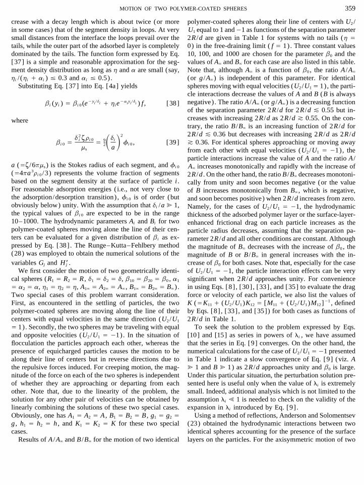
crease with a decay length which is about twice (or more polymer-coated spheres along their line of centers with U2 /U1 equal to 1 and01 as functions of the separation parameterin some cases) that of the segment density in loops. At very

small distances from the interface the loops prevail over the 2R /d are given in Table 1 for systems with no tails (h Å0) in the free-draining limit ( f Å 1). Three constant valuestails, while the outer part of the adsorbed layer is completely

dominated by the tails. The function form expressed by Eq. 10, 100, and 1000 are chosen for the parameter b0 and thevalues of A` and B` for each case are also listed in this table.[37] is a simple and reasonable approximation for the seg-

ment density distribution as long as h and a are small (say, Note that, although A` is a function of b0 , the ratio A /A`

(or g /A`) is independent of this parameter. For identicalhi / (hi / ai ) ° 0.3 and ai ° 0.5) .Substituting Eq. [37] into Eq. [4a] yields spheres moving with equal velocities (U2 /U1Å 1), the parti-

cle interactions decrease the values of A and B (B is alwaysnegative) . The ratio A /A` (or g /A`) is a decreasing functionbi (yi ) Å bi 0(e0yi /di / hi e

0ai yi /di ) f , [38]of the separation parameter 2R /d for 2R /d © 0.55 but in-creases with increasing 2R /d as 2R /d ™ 0.55. On the con-wheretrary, the ratio B /B` is an increasing function of 2R /d for2R /d © 0.36 but decreases with increasing 2R /d as 2R /d™ 0.36. For identical spheres approaching or moving awaybi 0 Å

d 2i zri 0

ms

Å 92Sdi

a D2

fi 0 , [39]from each other with equal velocities (U2 /U1 Å 01), theparticle interactions increase the value of A and the ratio A /

a (Åz /6pms ) is the Stokes radius of each segment, and fi 0 A` increases monotonically and rapidly with the increase of(Å4pa 3ri 0 /3) represents the volume fraction of segments 2R /d . On the other hand, the ratio B /B` decreases monotoni-based on the segment density at the surface of particle i . cally from unity and soon becomes negative (or the valueFor reasonable adsorption energies (i.e., not very close to of B increases monotonically from B` , which is negative,the adsorption/desorption transition), fi 0 is of order (but and soon becomes positive) when 2R /d increases from zero.obviously below) unity. With the assumption that di /a @ 1, Namely, for the cases of U2 /U1 Å 01, the hydrodynamicthe typical values of bi 0 are expected to be in the range thickness of the adsorbed polymer layer or the surface-layer-10–1000. The hydrodynamic parameters Ai and Bi for two enhanced frictional drag on each particle increases as thepolymer-coated spheres moving alone the line of their cen- particle radius decreases, assuming that the separation pa-ters can be evaluated for a given distribution of bi as ex- rameter 2R /d and all other conditions are constant. Althoughpressed by Eq. [38]. The Runge–Kutta–Fehlbery method the magnitude of B` decreases with the increase of b0 , the(28) was employed to obtain the numerical solutions of the magnitude of B or B /B` in general increases with the in-

crease of b0 for both cases. Note that, especially for the casevariables Gj and H*j .We first consider the motion of two geometrically identi- of U2 /U1 Å 01, the particle interaction effects can be very

significant when 2R /d approaches unity. For conveniencecal spheres (R1 Å R2 Å R , d1 Å d2 Å d, b10 Å b20 Å b0 , a1

Å a2 Å a, h1 Å h2 Å h, A1` Å A2` Å A` , B1` Å B2` Å B`) . in using Eqs. [8] , [30], [33], and [35] to evaluate the dragforce or velocity of each particle, we also list the values ofTwo special cases of this problem warrant consideration.

First, as encountered in the settling of particles, the two K (ÅK11 / (U2 /U1)K12 Å [M11 / (U2 /U1)M12]01 , definedby Eqs. [8] , [33], and [35]) for both cases as functions ofpolymer-coated spheres are moving along the line of their

centers with equal velocities in the same direction (U2 /U1 2R /d in Table 1.To seek the solution to the problem expressed by Eqs.Å 1). Secondly, the two spheres may be traveling with equal

and opposite velocities (U2 /U1 Å 01). In the situation of [10] and [15] as series in powers of li , we have assumedthat the series in Eq. [9] converges. On the other hand, theflocculation the particles approach each other, whereas the

presence of equicharged particles causes the motion to be numerical calculations for the case of U2 /U1 Å 01 presentedin Table 1 indicate a slow convergence of Eq. [9] (viz. Aalong their line of centers but in reverse directions due to

the repulsive forces induced. For creeping motion, the mag- @ 1 and B @ 1) as 2R /d approaches unity and b0 is large.Under this particular situation, the perturbation solution pre-nitude of the force on each of the two spheres is independent

of whether they are approaching or departing from each sented here is useful only when the value of li is extremelysmall. Indeed, additional analysis which is not limited to theother. Note that, due to the linearity of the problem, the

solution for any other pair of velocities can be obtained by assumption li ! 1 is needed to check on the validity of theexpansion in li introduced by Eq. [9] .linearly combining the solutions of these two special cases.

Obviously, one has A1 Å A2 Å A , B1 Å B2 Å B , g1 Å g2 Å Using a method of reflections, Anderson and Solomentsev(23) obtained the hydrodynamic interactions between twog , h1 Å h2 Å h , and K1 Å K2 Å K for these two special

cases. identical spheres accounting for the presence of the surfacelayers on the particles. For the axisymmetric motion of twoResults of A /A` and B /B` for the motion of two identical

AID JCIS 5144 / 6g34$$$305 12-09-97 15:09:56 coidas

360 KUO AND KEH

TABLE 1Numerical Results of A/A` and B/B` for Two Identical Polymer-Coated Spheres Moving along the Line of Their Centers with

Various Values of Parameters 2R/d, b0, and U2/U1 for Systems with No Polymer Tails in the Free-Draining Limit

B/B`

A/A` b0 Å 10 b0 Å 100 b0 Å 1000 K

2Rd

U2

U1

Å 1U2

U1

Å 01U2

U1

Å 1U2

U1

Å 01U2

U1

Å 1U2

U1

Å 01U2

U1

Å 1U2

U1

Å 01U2

U1

Å 1U2

U1

Å 01

0 1 1 1 1 1 1 1 1 1 10.1 0.9307 1.0808 1.2499 0.7077 1.6937 0.1884 2.3595 00.5907 0.9303 1.08100.2 0.8733 1.1746 1.4403 0.3725 2.2244 00.7479 3.4007 02.4287 0.8706 1.17560.3 0.8296 1.2863 1.5443 00.0274 2.5166 01.8793 3.9755 04.6577 0.8198 1.28780.4 0.8011 1.4264 1.5441 00.5431 2.5163 03.3644 3.9748 07.5974 0.7772 1.42420.5 0.7881 1.6160 1.4566 01.2764 2.2640 05.5176 3.4753 011.881 0.7422 1.59670.6 0.7875 1.9002 1.3426 02.4411 1.9275 08.9978 2.8050 018.835 0.7140 1.82830.7 0.7942 2.3916 1.2678 04.5548 1.6969 015.397 2.3407 031.665 0.6913 2.17080.8 0.8028 3.4557 1.2350 09.2079 1.5894 029.596 2.1212 060.186 0.6729 2.77240.9 0.8115 7.1185 1.2116 024.370 1.5137 075.985 1.9668 0153.42 0.6578 4.33310.95 0.8157 15.486 1.2020 055.628 1.4825 0171.58 1.9035 0345.55 0.6512 7.14160.99 0.8190 — 1.1967 — 1.4656 — 1.8690 — 0.6475 15.498

A` Å 3.4570 A` Å 5.7596 A` Å 8.0622B` Å 00.9509 B` Å 00.5712 B` Å 00.4081

spheres with U2 /U1 equal to 1 and 01 considered here, their 01, and various values of the size ratio R2 /R1 are plottedresults give versus the separation parameter (R1 / R2) /d in Fig. 2 for

systems with no tails in the free-draining limit. The parame-ters A2 /A2` and B2 /B2` for the case of R2 /R1 Å x are equal

A Å A`KF1 / 2j 3 / 454

j 4 / O(j 6)G , [40a] to A1 /A1` and B1 /B1` , respectively, for the case of R2 /R1 Å1/x. Similar to the case of two identical polymer-coatedspheres, Ai /Ai` increases and Bi /Bi` decreases with the in-A 2 0 AB Å KFA 2

` 0 A`B` / 12(A 2

` 0 A`B` / 6V`)crease of (R1 / R2) /d . In general, the influence of the parti-cle interaction is more significant on the ratios Ai /Ai` andBi /Bi` of the larger particle than on those of the smaller one.1 SU2

U1Dj 3 0 45

4(A 2

` / 2A`B`)j 4 / O(j 6)G , [40b]We next consider the effect of tails in the surface layers

of two identical polymer-coated spheres. Equations [23] andwhere j Å R /d and the definition of V` has been given by[25] are solved for Gj and H *j in the free-draining limit overEq. [28d]. The normalized values of A and A 2 0 AB calcu-a range of h and a. For the situation of U2 /U1 Å 01, thelated from the above asymptotic solution, with the O(j 6)results of parameters B and h as functions of the ratio 2R /terms neglected, are compared with our results in Table 2.d are plotted in Fig. 3 for typical cases of the fraction ofIt can be found that the asymptotic formulas from the methodpolymer segments contained in the tails, h / (h / a) . Theof reflections shown in Eq. [40] agree well with the exactcurve of parameter A (or g) is not drawn since the ratio A /results as long as the particle surfaces are more than the sumA` is not a function of h / (h / a) or a and its results wereof radii apart ( i.e., 2R /d õ 0.5) . However, accuracy beginspresented in Table 1. It can be seen that the increase of theto deteriorate, as expected, when the particles are close to-segment fraction in the tails or the increase of the relativegether.length of the tails (with a decrease in a) will increase theBecause many suspensions in practical applications areparticle interaction effect on B and h when all the othercomposed of particles of different sizes, it might be of inter-conditions are unchanged. This influence can be quite sig-est to examine the interactions between two polymer-coatednificant when the value of a is less than 0.5. It implies thatspheres with identical characteristics in the surface layersthe interaction between colloidal particles in the presence of(d1 Å d2 Å d and b10 Å b20 Å b0) but with unequal radii.adsorbed polymers is to a large extent determined by longThe results of A1 /A1` and B1 /B1` for the motion of two

spheres along their line of centers with b0 Å 100, U2 /U1 Å dangling tails.

AID JCIS 5144 / 6g34$$$305 12-09-97 15:09:56 coidas


TABLE 2The Normalized Values of A and A2 0 AB for Two Identical Polymer-Coated Spheres Moving along The Line of Their Centers

with Various Values of Parameters 2R/d, b0, and U2/U1 for Systems with No Polymer Tails in the Free-Draining Limit, As Computedfrom Our Collocation Method (Listed in Column KK) and from Eq. [40] (Listed in Column AS)

(A2 0 AB)/(A2` 0 A`B`)

A/A` b0 Å 10 b0 Å 100 b0 Å 1000

2R/d KK AS KK AS KK AS KK AS

U2/U1 Å 10.1 0.9307 0.9307 0.9303 0.9302 0.9302 0.9302 0.9302 0.93020.2 0.8733 0.8733 0.8695 0.8694 0.8691 0.8690 0.8690 0.86890.3 0.8296 0.8301 0.8161 0.8156 0.8145 0.8137 0.8140 0.81310.4 0.8011 0.8037 0.7702 0.7665 0.7658 0.7608 0.7642 0.75910.5 0.7881 0.7982 0.7347 0.7202 0.7260 0.7069 0.7231 0.70280.6 0.7875 0.8176 0.7145 0.6737 0.7012 0.6473 0.6966 0.63900.7 0.7942 0.8673 0.7119 0.6241 0.6954 0.5766 0.6899 0.56180.8 0.8028 0.9528 0.7193 0.5674 0.7015 0.4885 0.6955 0.46400.9 0.8115 1.0812 0.7286 0.5000 0.7099 0.3765 0.7037 0.33820.95 0.8157 1.1637 0.7333 0.4612 0.7145 0.3094 0.7081 0.26230.99 0.8190 1.2396 1.1967 0.4139 1.4656 0.2495 1.8690 0.1945

U2/U1 Å 010.1 1.0808 1.0808 1.0811 1.0811 1.0811 1.0811 1.0811 1.08110.2 1.1746 1.1746 1.1764 1.1764 1.1759 1.1759 1.1758 1.17570.3 1.2863 1.2865 1.2900 1.2896 1.2872 1.2868 1.2862 1.28590.4 1.4264 1.4269 1.4286 1.4264 1.4181 1.4168 1.4145 1.41360.5 1.6160 1.6169 1.6031 1.5969 1.5713 1.5705 1.5606 1.56160.6 1.9002 1.8960 1.8312 1.8187 1.7423 1.7560 1.7124 1.73500.7 2.3916 2.3509 2.1359 2.1344 1.8813 1.9964 1.7955 1.95020.8 3.4557 3.2160 2.5013 2.6681 1.6366 2.3675 1.3458 2.26680.9 7.1185 5.5419 2.3178 4.0224 02.7019 3.2698 04.3869 3.01770.95 15.486 9.7025 2.2430 6.4651 021.559 4.9249 029.559 4.4089

action effect on B and h increases when the value of d /a isWe have also numerically solved for Gj and H*j for thedecreased for a given value of b0 , the hydrodynamic interac-system with no tails in the adsorbed polymer layers consider-tions among the polymer segments produce relatively smalling the hydrodynamic interactions among the polymer seg-effects on B and h .ments. In the calculations, we follow Anderson and Kim

(21) and use a combination of a modified Brinkman equationat low fi and the Blake–Kozeny equation at high fi for the CONCLUDING REMARKSexpression of function f (fi ) :

The slow motion of two spherical particles coated withf Å 1 / 2.121f 1/2

i / 0.84filn fi / 16.456fi adsorbed polymer layers has been analyzed in this work.The analysis provides governing equations and boundaryfor fi õ 0.29, [41a]conditions which must be solved, given the polymer segmentdensity distribution r(yi ) and rheological parameters m(yi )f Å 8.34fi

(1 0 fi )3 for fi ú 0.29, [41b]and bi (yi ) , to determine the parameters Ai and Bi of Eq.[9] or parameters gi and hi of Eq. [30]. The hydrodynamic

where fi Å (43)pa 3r(yi ) . For two identical polymer-coated forces exerted on the particles for a resistance problem or

the particle velocities for a mobility problem correct tospheres, the ratio A /A` (or g /A`) is independent of f (fi )( in spite of the fact that A` is a weak function of d /a) and O(l2

i ) can be calculated using Eq. [33] or [35] and theresults of Ai and Bi . For the exponential polymer segmentits results are the same as those given in Table 1. In Fig. 4,

the results of parameters B and h for two spheres with U2 / distribution given by Eq. [37], the ratio A /A` or g /A` oftwo identical spheres is found to be independent of the valuesU1 Å 01 versus 2R /d obtained using Eq. [41] are plotted

for various values of b0 and d /a . Although the particle inter- of b0 , d /a , a, and h / (h / a) , and its results for various

AID JCIS 5144 / 6g34$$$305 12-09-97 15:09:56 coidas

362 KUO AND KEH

r(yi ) Å ri 0e0yi /di

1 / s(yi /Ri ), i Å 1, 2, [42]

where s should be a positive value. For two identical poly-mer-coated spheres with no tails in the free-draining limit,b(y) has the form of the above equation with ri 0 replacedby b0 . It is understood that parameters A` and A (or g) areindependent of the curvature coefficient s . We have numeri-cally solved Eqs. [23] and [25] with the segment distribu-tion given by Eq. [42] and substituted the solution of Gj

and H *j into Eq. [27b] to compute parameters B and h .

FIG. 2. The normalized parameters A1 /A1` and B1 /B1` for the motionof two polymer-coated spheres with d1 Å d2 , b10 Å b20 Å 100, U2 /U1 Å01, and various values of the size ratio R2 /R1 as a function of the separationparameter (R1 / R2) /d in the free-draining limit ( f Å 1).

values of 2R /d are listed in Table 1. The dependence of Band h on b0 , d /a , a, h / (h / a) , and R /2d is given in Table1 and Figs. 3 and 4. The results indicate that the particleinteraction effects on the motion of two polymer-coated par-ticles can be significant.

Throughout the calculations in the previous section wehave assumed a simple exponential decay of the polymersegment density. This could be an oversimplification sincethe convex nature of the surfaces of the particles might adjust

FIG. 3. The parameters B and h for the motion of two identical polymer-the excluded volume effects among the polymer segments. coated spheres with b0 Å 100 and U2 /U1 Å 01 as a function of 2R /d inA segment density of the following form was suggested (21) the free-draining limit ( f Å 1). The solid curves are plotted for the case

of a Å 0.5, and the dashed curves are plotted for the case of a Å 0.25.to allow for curvature effects on polymer distribution:

AID JCIS 5144 / 6g34$$$306 12-09-97 15:09:56 coidas


r(yi ) Å 0 if yi ú di . [43b]

For this profile in the free-draining limit, bi (yi ) has the formof Eq. [43] with ri 0 replaced by bi 0 and it can be shownthat

Ai` Å 1 0 b01/2i 0 tanh b 1/2

i 0 , [44a]

Bi` Å 01

Ai`bi 0

(1 0 sech b 1/2i 0 ) 2 . [44b]

It can be found that the value of Ai` is about six times greater

FIG. 4. The parameters B and h for the motion of two identical polymer-coated spheres with U2 /U1 Å 01 as a function of 2R /d . The solid curvesare plotted for the case of b0 Å 10, and the dashed curves are plotted forthe case of b0 Å 100. Note that d /a r ` represents the free-draining limit( f Å 1) and the two dashed curves are almost indistinguishable.

These calculations, which are plotted in Fig. 5 for the caseof U2 /U1 Å 01, indicate that the magnitudes of B and hdecrease with the increase of s for various values of 2R /das one would expect.

One may wish to consider a polymer segment distributionthat has the same adsorbed amount as for the exponentialdistribution but is uniform over a distance from the particlesurface:

FIG. 5. The parameters B and h for the motion of two identical polymer-coated spheres with the segment density distribution given by Eq. [42], b0

Å 100, and U2 /U1 Å 01 as a function of 2R /d in the free-draining limit.r(yi ) Å ri 0 if 0 ° yi ° di , [43a]

AID JCIS 5144 / 6g34$$$306 12-09-97 15:09:56 coidas

364 KUO AND KEH

can be seen that the particle interaction effect on B and h isweaker for the uniform distribution of segments over a dis-tance from the particle surface than for the exponential distri-bution of segments.

In addition to obtaining suitable approximate solutions ofthe quasisteady equations of motion of two polymer-coatedspheres, it is desirable to know how well the predicted effectswill be realized physically. Although experimental work haslagged behind the theory in this area, considerable data for twomutually interacting ‘‘bare’’ spheres are now available whichindicate good agreement with corresponding solutions of thecreeping motion equations (25). Once the segment densitydistribution in the surface polymer layer r(y) together withthe dimensionless surface density parameter b0 is determinedindependently, one can measure the velocities and drag forcesexperienced by two polymer-coated spheres falling along theline between their centers in a viscous fluid for various valuesof the separation parameter (29) and choose the values of li

to test the theoretical analysis developed in this work.

APPENDIX A

For completeness the definitions of functions Wik(ni ) ,Xik(ni ) , Yik(ni ) , and Zik(ni ) in Eq. [19] are listed here.

Wik(ni ) Å ∑`

nÅ2H[R0n/1

i Cink / R0n/3i Dink]G01/2

n (ni )

/ Slj

liDk

[g0n/1ij Cjnk / g0n/3

ij Djnk]Gn0ijJ , [A.1]

Xik(ni ) Å ∑`

nÅ2H0[(n 0 1)R0n

i Cink / (n 0 3)R0n/2i Dink]

1 G01/2n (ni ) / Slj

liDk/1

g0n/1ij [Gn1ij

FIG. 6. The parameters B and h for the motion of two identical polymer-coated spheres with the segment density distribution given by Eq. [43], b0

Å 100, and U2 /U1 Å 01 as a function of 2R /d in the free-draining limit. 0 (n 0 1)hijGn0ij]Cjnk / Slj

liDk/1

g0n/3ijThe corresponding results for the exponential segment distribution are also

plotted for comparison.

1 [Gn1ij 0 (n 0 3)hijGn0ij]DjnkJ , [A.2]

( if bi 0 É 100) for an exponential distribution of segmentsthan for the polymer uniformly distributed over a region ofthickness di . Although Ai` is a function of bi 0 for this seg- Yik(ni )Å ∑

`

nÅ2H 1

2[n(n0 1)R0n01i Cink

ment distribution, the ratio Ai /Ai` or gi /Ai` for the motionof two polymer-coated spheres is independent of the segment / (n0 2)(n0 3)R0n/1

i Dink]G01/2n (ni )

distribution, and its results have been given in Table 1 andFig. 2. In Fig. 6, the numerical results of parameters B and / Slj

liDk/2

g0n/1ij FGn2ij0 (n0 1)hijGn1ijh obtained using Eq. [43] as the segment distribution are

plotted for the case of U2 /U1 Å 01. The correspondingresults for the case of the exponential distribution of seg- / (n0 1)S n

2h 2

ij0mijDGn0ijGCjnkments are also plotted in the same figure for comparison. It

AID JCIS 5144 / 6g34$$$306 12-09-97 15:09:56 coidas


/ Slj

liDk/2

g0n/3ij FGn2ij0 (n0 3)hijGn1ij Gn3ij Å

16(2n 0 1) H 1

2 n03 ∑»n02 …

kÅ0

1 (01) k(n 0 k 0 2)!k!(n 0 2k 0 3)!(n 0 k 0 2)!

t n02k02ij/ (n0 3)S n0 2

2h 2

ij0mijDGn0ijGDjnkJ , [A.3]

1 [(n 0 2k 0 3)(n 0 2k 0 4)u 3ij

Zik(ni ) Å ∑`

nÅ2H01

6(n 0 1)[n(n / 1)R0n02i Cink / 6(n 0 2k 0 3)uij£ij / 6wij] 0

12 n01

/ (n 0 2)(n 0 3)R0ni Dink]G01/2

n (ni ) 1 ∑»n …

kÅ0

(01) k(n 0 k)!k!(n 0 2k 0 1)!(n 0 k)!

t n02kij

/ Slj

liDk/3

g0n/1ij FGn3ij 0 (n 0 1)hijGn2ij 1 [(n 0 2k 0 1)(n 0 2k 0 2)u 3

ij

/ 6(n 0 2k 0 1)uij£ij / 6wij]J , [A.8]/ (n 0 1)S n

2h 2

ij 0 mijDGn1ij 0 (n 0 1)

and1 S n(n / 1)6

h 3ij 0 nhijmij / nijDGn0ijGCjnk

gij Å x 1/2ij , [A.9]

/ Slj

liDk/3

g0n/3ij FGn3ij 0 (n 0 3)hijGn2ij

hij Å x01ij yij , [A.10]

mij Å 012x02

ij y 2ij / 1

2x01ij , [A.11]

/ (n 0 3)S n 0 22

h 2ij 0 mijDGn1ij

nij Å 12x03

ij y 3ij 0 1

2x02ij yij . [A.12]

0 (n 0 3)S (n 0 1)(n 0 2)6

h 3ij In Eqs. [A.5] – [A.8], »n … Å 0 if n Å 0, »n … Å (n 0 1)/2

if n is odd, »n … Å (n 0 2)/2 if n is even, and0 (n 0 2)hijmij / nijDGn0ijGDjnkJ , [A.4]

tij Å x01/2ij zij , [A.13]

where j Å 3 0 i , uij Å ni z01ij 0 x01

ij yij , [A.14]Gn0ij Å G01/2

n ( tij) , [A.5]£ij Å 3

2x02ij y 2

ij 0 12x01

ij 0 ni x01ij yijz

01ij , [A.15]

Gn1ijÅ1

(2n0 1) H 12 n03 ∑

»n02 …

kÅ0wij Å 05

2x03ij y 3

ij / 32x02

ij yij

/ 32ni x02

ij y 2ij z01ij 0 1

2ni x01ij z01

ij . [A.16]1 (01) k(n0 k0 2)!

k!(n0 2k0 3)!(n0 k0 2)!t n02k02

ij uij01

2 n01

In Eqs. [A.9] – [A.16],1 ∑

»n …

kÅ0

(01) k(n0 k)!k!(n0 2k0 1)!(n0 k)!

t n02kij uijJ , [A.6]

xij Å R 2i / ( j 0 i)(3 0 2i)d 2 0 2( j 0 i)Rini d , [A.17]

yij Å Ri 0 ( j 0 i)ni d , [A.18]Gn2ij Å1

2(2n 0 1) H 12 n03 ∑

»n02 …

kÅ0zij Å Rini 0 ( j 0 i)d . [A.19]

1 (01) k(n 0 k 0 2)!k!(n 0 2k 0 3)!(n 0 k 0 2)!

t n02k02ij

APPENDIX B: NOMENCLATURE

1 [(n 0 2k 0 3)u 2ij / 2£ij] 0

12 n01 a Stokes radius of a polymer segment (m)

Ai` , Bi` parameters defined by Eq. [29]1 ∑

»n …

kÅ0

(01) k(n 0 k)!k!(n 0 2k 0 1)!(n 0 k)!

t n02kij Ai , Bi parameters defined by Eq. [9]

bjn , cjn , djn coefficients defined by Eq. [20]Cin , Din coefficients defined by Eq. [10] (mn/2 /s,1 [(n 0 2k 0 1)u 2

ij / 2£ij]J , [A.7]mn /s)

AID JCIS 5144 / 6g34$$$307 12-09-97 15:09:56 coidas

366 KUO AND KEH

Cinm , Dinm coefficients defined by Eq. [11] (mn/2 /s, z Stokes friction coefficient of a polymersegment (kg/s)mn /s)

d center-to-center distance between two hi fraction of tails as defined by Eq. [38]ui , f angular spherical coordinates about parti-particles (m)

ez unit vector in the z direction cle ili di /Rif parameter for the hydrodynamic interac-

tions among polymer segments defined coefficients defined by Eqs. [30b, c]L *j , Lj

by Eq. [1a] m viscosity inside the polymer layer (kg/m s)Fi hydrodynamic force exerted on particle i ms fluid viscosity (kg/m s)

(N) ni cos ui

Finm functions of yi defined by Eq. [15] (m2) j R /dhydrodynamic force defined by Eq. [34]FJ (0)

j r polymer segment distribution (m03)(N) ri 0 polymer segment density in loops at the

gi , hi parameters defined by Eq. [30] surface of particle i (m03)functions of yj defined by Eqs. [22] – [26]Gj , Hj , H*j fi (4/3)pa 3r(yi )

(m) fi 0 (4/3)pa 3ri 0

Gegenbauer polynomials of order n andG01/2n C Stokes stream function (m3/s)

degree 012 C (O ) stream function in the outer region (m3/s)

Ki particle interaction factor defined by Eq. stream function in the inner region aboutC ( I )i

[8] particle i (m3/s)Kij dimensionless resistance coefficients de- radial cylindrical coordinate (m)v

V

fined by Eq. [33] Vj coefficients defined by Eq. [28d]Li effective hydrodynamic thickness of the

polymer layer on particle i defined byACKNOWLEDGMENT

Eq. [8] (m)Li` effective hydrodynamic thickness of the This work was supported by the National Science Council of the Republic

polymer layer on particle i defined by of China.Eq. [31] (m)

Mij dimensionless mobility coefficients de-REFERENCES

fined by Eq. [35]p hydrodynamic pressure (N/m2) 1. Napper, D. H., ‘‘Polymeric Stabilization of Colloidal Dispersions.’’pijn , qijn , sijn coefficients defined by Eq. [20] Academic Press, London, 1983.

2. Hunter, R. J., ‘‘Foundations of Colloid Science,’’ Vol. 1. ClarendonPn Legendre polynomial of order nPress, Oxford, 1986.ri radial spherical coordinate about particle

3. Roe, R. J., J. Chem. Phys. 44, 4264 (1966).i (m)4. Hesselink, F. Th., J. Colloid Interface Sci. 50, 606 (1975).

Ri radius of particle i (m) 5. Scheutjens, J. M. H. M., and Fleer, G. J., J. Phys. Chem. 84, 178s curvature coefficient defined by Eq. [42] (1980).

6. Fleer, G. J., Cohen Stuart, M. A., Scheutjens, J. M. H. M., Cosgrove,Ui translational velocity of particle i (m/s)T., and Vincent, B., ‘‘Polymers at Interfaces.’’ Chapman & Hall, Lon-velocity of particle j defined by Eq. [36]UJ (0)

jdon, 1993.(m/s)

7. Garvey, M. J., Tadros, Th. F., and Vincent, B., J. Colloid Interfacev fluid velocity (m/s) Sci. 55, 440 (1976).v (p ) velocity of polymer segments (m/s) 8. Kato, T., Nakamura, K., Kawaguchi, M., and Takahashi, A., Polym. J.

13, 1037 (1981).Wik , Xik , Yik , Zik functions of ni defined by Eqs. [A.1] –9. Cohen Stuart, M. A., Waajen, F. H. W. H., Cosgrove, T., Vincent, B.,[A.4] (m3/s, m2/s, m/s, s01)

and Crowley, T. L., Macromolecules 17, 1825 (1984).yi l01i (ri 0 Ri ) (m)

10. Baker, J. A., and Berg, J. C., Langmuir 4, 1055 (1988).z axial coordinate (m) 11. Koopal, L. K., Hlady, V., and Lyklema, J., J. Colloid Interface Sci.ai ratio of loop-to-tail length scales for the 121, 49 (1988).

12. Siffert, B., and Li, J. F., Colloids Surf. 62, 307 (1992).polymer layer of particle i13. Garvey, M. J., Tadros, Th. F., and Vincent, B., J. Colloid Interfacebi parameters defined by Eq. [4a]

Sci. 49, 57 (1974).bi 0 parameters defined by Eq. [39]14. Kawaguchi, M., and Takahashi, A., Adv. Colloid Interface Sci. 37, 219

gj coefficients defined by Eq. [28a] (1992).di length scale of the polymer layer sur- 15. Doroszkowski, A., and Lambourne, R., J. Colloid Interface Sci. 26,

214 (1968).rounding particle i (m)

AID JCIS 5144 / 6g34$$$308 12-09-97 15:09:56 coidas


16. Barsted, S. J., Nowakowska, L. T., Wagstaff, I., and Walbridge, D. J., 23. Anderson, J. L., and Solomentsev, Y., Chem. Eng. Commun. 148–150,291 (1996).Trans. Faraday Soc. 67, 3589 (1971).

24. Gluckman, M. J., Pfeffer, R., and Weinbaum, S., J. Fluid Mech. 50,17. Varoqui, R., and Dejardin, P., J. Chem. Phys. 66, 4395 (1977).705 (1971).18. Stromberg, R. R., Tutas, D. J., and Passaglia, E., J. Phys. Chem. 69,

25. Happel, J., and Brenner, H., ‘‘Low Reynolds Number Hydrodynam-3955 (1965).ics.’’ Martinus Nijhoff, Dordrecht, The Netherlands, 1983.

19. Lee, J. J., and Fuller, G. G., J. Colloid Interface Sci. 103, 569 (1985).26. Baker, J. A., Pearson, R. A., and Berg, J. C., Langmuir 5, 339 (1989).

20. Barnett, K. G., Cosgrove, T., Vincent, B., Burgess, A. N., Crowley, 27. Keh, H. J., and Tseng, Y. K., AIChE J. 38, 1881 (1992).T. L., King, T., Turner, J. D., and Tadros, Th. F., Polymer 22, 283 28. Gerald, C. F., and Wheatley, P. O., ‘‘Applied Numerical Analysis,’’(1981). 5th ed. Addison-Wesley, Reading, MA, 1994.

21. Anderson, J. L., and Kim, J., J. Chem. Phys. 86, 5163 (1987). 29. Steinberger, E. H., Pruppacher, H. R., and Neiburger, M., J. FluidMech. 34, 809 (1968).22. Keh, H. J., and Kuo, J., J. Colloid Interface Sci. 185, 411 (1997).

AID JCIS 5144 / 6g34$$$308 12-09-97 15:09:56 coidas

Documents

Effects of Adsorbed Polymers on the Axisymmetric Motion of Two Colloidal Spheres