Effects of chinsaga (gynandropsis gynandra) On

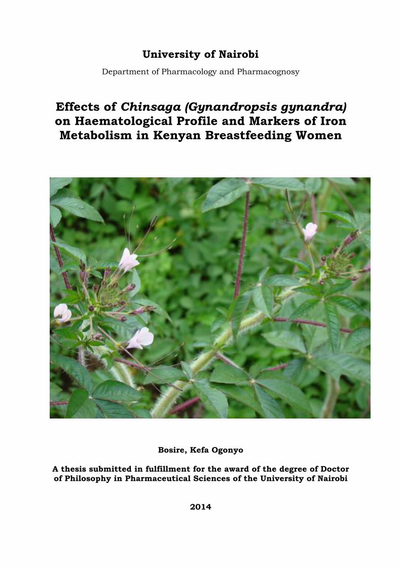
University of Nairobi

Department of Pharmacology and Pharmacognosy

Effects of Chinsaga (Gynandropsis gynandra) on Haematological Profile and Markers of Iron Metabolism in Kenyan Breastfeeding Women

Bosire, Kefa Ogonyo

A thesis submitted in fulfillment for the award of the degree of Doctor of Philosophy in Pharmaceutical Sciences of the University of Nairobi

2014

~ ii ~

Declaration

I hereby declare that this research thesis is my original work and has not

been presented to any other academic institution for evaluation for research

and examination.

Signature___________________________ Date______________________

Supervisors’ Approval

This research thesis has been submitted for evaluation for research and

examination with our approval as university supervisors.

1. PROF. ANASTASIA NKATHA GUANTAI, PhD

Department of Pharmacology and Pharmacognosy, University of Nairobi

Signature_______________________________ Date_____________________

2. DR. FAITH OKALEBO, PhD


Signature_________________________________ Date________________________

3. DR. GEORGE OYAMO OSANJO, PhD


Signature_______________________________ Date______________________

~ iii ~

UNIVERSITY OF NAIROBI

Declaration of Originality Form

This form must be completed and signed for all works submitted to the University for

examination.

Name of Student __________Kefa Ogonyo Bosire___________________________________

Registration Number ______U80/8763/06_________________________________________

College ___________________Health Sciences______________________________________

Faculty/School/Institute___Pharmacy____________________________________________

Department _______________Pharmacology and Pharmacognosy___________________

Course Name _____________Doctor of Philosophy in Pharmaceutical Sciences ____

Title of the work:

Effect Of Gynandropsis Gynandra (Chinsaga) on Haematological Profile and Markers

of Iron Metabolism in Kenyan Lactating Women.

DECLARATION

1. I understand what Plagiarism is and I am aware of the University’s policy in this regard

2. I declare that this Thesis is my original work and has not been submitted elsewhere for

examination, award of a degree or publication. Where other people’s work, or my own work

has been used, this has properly been acknowledged and referenced in accordance with the University of Nairobi’s requirements.

3. I have not sought or used the services of any professional agencies to produce this work

4. I have not allowed, and shall not allow anyone to copy my work with the intention of

passing it off as his/her own work

5. I understand that any false claim in respect of this work shall result in disciplinary

action, in accordance with University Plagiarism Policy.

Signature _____________________________________________

Date _______________________________________________________

~ iv ~

Foreword The genesis of this work was not a result of painstaking innovation as an

individual but rather a product of ideas shared and experiences gained

during my upbringing. The knowledge and selection of this subject for study

was motivated by a deep desire to explore the richness of cultural

knowledge and the fascination with the diversity of plants used by different

communities as interventions during sickness and more importantly, in

promotive health. Several ideas were explored eventually leading to

selection of the current study as a model for validating our traditional

knowledge and practices related to health. Unfortunately, the knowledge

gained over centuries and initially passed on by oral tradition is getting

eroded by westernization of our societies.

The opportunity for interaction with the Kisii culture and exposure to many

others has helped shape my development of a comparative map of the

cultural practices among communities in our country. This has provided

the basis for identifying similarities and distinctions related to health

promotion. My hope is that this work will stimulate and encourage

documentation and evaluation of our heritage for future generations.

~ v ~

Abstract

Introduction: Chinsaga (Gynandropsis gynandra (L.)) is a leafy vegetable

indigenous to Africa, and is an important component of the traditional diet

of the people of western Kenya such as the Abagusii, who refer to it as

Chinsaga. The Abagusii believed Chinsaga has powerful blood restorative

properties, and is recommended for pregnant and lactating women as a

hematinic and immunostimulant.

Objective: This study sought to provide scientific validation for the

traditional use of Gynandropsis gynandra (L.) among the Kisii community

(Abagusii) in promoting maternal and child nutrition. This was done by

assessing the impact of Gynandropsis gynandra (Chinsaga) consumption on

the hematological profile and selected iron metabolism biomarkers among

lactating women at Kenyatta National Hospital as indicators of nutritional

status. The study also aimed at documenting the socioeconomic value of

Chinsaga and chromatographic characterization of the plant sourced from

Kilgoris and Kisii.

Methodology: A cross-sectional survey was undertaken to examine the

socioeconomic value and trade of Chinsaga in Kisii and Kilgoris followed by

plant collection and processing to provide material for a clinical study. A

sample of the processed material was subjected to chromatographic

characterization using Thin Layer (TLC) and High Performance Liquid

(HPLC) Chromatography.

The study was reviewed and granted ethics approval by the Kenyatta

National Hospital – University of Nairobi Ethics and Research Committee

(KNH-UoN ERC), reference number: KNH-ERC/01/3757. A randomized

triple blind controlled study was carried out at Kenyatta National Hospital

Maternal Child Health Clinic 17. The study enrolled 119 women below 35

years of age, with a maximum of 4 live births and between their first and

~ vi ~

second month after delivery. The two arm study evaluated the effects of

Chinsaga consumption on hematological profile and on selected markers of

iron metabolism. The comparator intervention was dietary supplementation

with processed kale (Brassica carinata). Participants were followed for 28

days and anthropometrics, demographics, blood and milk specimens were

collected. The pre and post treatment hematological laboratory parameters

tested included; ferritin, transferritin and lactoferrin as biomarkers of iron

metabolism.

Results: Chinsaga trade has a well structured supply chain with:

producers; collectors; wholesalers; retailers and consumers in a variety of

combinations. The highest demand is in urban areas. Commercial

agriculture of Chinsaga has good prospects; however farm sizes are

declining.

The plant undergoes three stages of maturation as described by farmers:

Omonyenye (germination to four weeks); Amasabore (week 4 to 8) and

Ekegoko, (mature stage). The Amasabore and Ekegoko are recommended for

lactating mothers. A chromatographic fingerprint of Chinsaga was

developed using ethyl acetate: methanol: water (50:20:10) on thin layer

chromatography (TLC) and greater resolution achieved using gradient

elution on HPLC-UV with acetonitrile, propan-2-ol, water and formic acid

(0.4%) in the ratios 85:35:25, adjusted to pH 2.3 as mobile phase on a C18

column.

In the clinical study involving lactating mothers, Chinsaga supplementation

was associated with significantly higher values of Red Blood Cell Counts

(RBC) in the 2nd visit (median 4.79 Interquatile Range (IQR) 4.51 – 5.05,

p=0.03) and 3rd visit (median 4.85, (IQR 4.46 – 5.18, p=0.03) compared to

the control arm. Similar differences across arms were observed with

changes in mean corpuscular volume; (median 27.3, IQR 25.5 – 29, p=0.03)

and hemoglobin concentration (median 27.5, IQR 25.85 – 28.85, p=0.05).

~ vii ~

However there were no statistically significant differences across arms for

hemotocrit, (median 39.2, IQR 33.9 – 40.3, p=0.31) and hemoglobulin

(median 13.3, IQR 11.7 – 13.85, p=0.42).

On stratified data analysis, the effects of Chinsaga are dependent on patient

reported duration of iron intake. The effects of Chinsaga on RBC count were

most prominent in patients who had taken iron supplements for at least 1

month. On bivariable generalized linear regression modeling, the other

variables that were positively associated with RBC counts and with p< 0.05

were; duration of stay at the current residence, age of husband, Njahe,

Ugali and Cocoa. However, on adjusting for confounding, only cocoa

consumption had a statistically negative effect on RBC counts (adjusted β -

6.735 ± 1.827 P=0.00).

At a molecular level, there was progressive increase in transferrin gene

expression during the three clinic visits. The highest mean was observed in

the third visit (2.3, 95% C I (4.49 , 0.170).

Conclusion and recommendations: This study confirms the cultural value

of Chinsaga and its socioeconomic benefit to the community of the Kisii by

providing scientific data supporting the folklore use of Chinsaga by

breastfeeding mothers for blood restoration as evidenced by the

improvement of the hematological profile and effects on markers of iron

metabolism. Chinsaga is a viable commercial crop that should be exploited

for the socioeconomic benefit of Kenyans. Studies are needed to examine

the effect of Chinsaga diet on enhancing breast milk quantity. This study

exposes a gap in the knowledge and the need to conduct similar studies on

traditional vegetables and foods consumed by various communities in

Kenya. Such action will help preserve what is known and promote the

incorporation of the traditional vegetables into the diet for the benefit of

mankind. In addition, this study has demonstrated feasibility and provided

a model for the design and conduct similar studies.

~ viii ~

Dedication

To Dr. Enoch Bosire Nyanusi and Mrs. Milkah Nyaboke Bosire; Naomi

Bosibori, Vanessa Yunuke, Hellen Mokeira, Walter Nyanusi, Edward,

Ombeng’i ;Caro, Irene, Emma; Eric, Oscar, Mark and Justo

~ ix ~

Acknowledgements

The work reported in this thesis is the culmination of concerted support by

many people to whom I owe much gratitude not reflected in this summary.

To this end, I therefore concede that I may not adequately capture all those

that played key roles at different steps but their contributions are highly

regarded.

Prof. Anastasia Guantai has been my mentor for over two decades and I owe

much to her for her unwavering patience. Her confidence in me was

important in getting the ideas on paper. I also thank her for the support

throughout the difficult years between and the final culmination in this

report. God bless her and her family.

It is many years since I lost a dear friend and mentor in the late Prof. Job

Bwayo then head of Kenya Aids Vaccine Initiative. I retain fond memories of

trainings as a clinical trials pharmacist and responsibilities given that

initiated my current participation in projects within the University of

Nairobi. May his inspiration live on to benefit others.

I also extend my deep gratitude to Professor Isaac Kibwage for the

consistent support beyond official duty that has helped see me overcome

challenges and enriched my experience both as a member of faculty and as

a postgraduate student.

The most notable blessing in having my mentors and supervisors was the

establishment of relationships extending beyond our official duties. This

has been very dear to me and my family.

I wish to express my sincere gratitude to Dr. Faith Okalebo who has been a

pillar of support right from my days as an undergraduate. Special thanks

for her key role in guiding me organize and analyze data and drafting of this

~ x ~

thesis. In a similar manner, I thank Dr. George Oyamo for his incisive

review of my work and support during the lab analysis. They made a great

team of advisors for which I will always owe my best regards.

During my fieldwork in Kisii and Kilgoris, I owe much of my success to Abel

of Mwalimu Hotel for introducing me to his cousin Eliud Mayaka who

executed efficiently the role of purchasing, cooking, drying and organizing

transport to Nairobi the vegetables used in this study. I could not thank

them both sufficiently through this paragraph.

The manager and his assistant at Nyankoba Tea Factory were extremely

kind to Eliud Mayaka and me by providing access to the wilting beds for

use in overnight drying of the cooked vegetables. The many failures we

experienced prior to this support are testimony to the importance of the

facility in making the preparations so much easier at a time of limited

sunshine and much rain.

I express sincere thanks to Mr. Josephat Mwalukumbi for sparing his time

to mill the dried materials and Betty for kindly rescheduling other contracts

at her company and giving my material priority for packing.

While conducting the clinical studies, I thank management at Kenya Aids

Vaccine Initiative, and staff at the laboratory for helping process and store

of blood and breast milk samples till ready for analysis.

At the Department of Obstetrics and Gynecology, I thank Prof. James Kiarie

for permission and Yonnie Otieno for helping to prepare the aliquots and

arranging for the import of the vitamin A analyzer from Germany.

Not least, I express my sincere gratitude to Jeremiah Zablon and Nathan

Shaviya for identifying laboratory space used to carry out the protein runs

analysis of the gels and interpretation of the results. They too have

~ xi ~

remained such committed friends ever reminding me to complete drafting

this thesis.

Within the School of Pharmacy, I thank all my colleagues and special

gratitude to Dr. Kennedy Abuga for his incisive advice throughout the years.

Similarly, I am grateful to the Dr. Hezekiah Chepkwony and the National

Quality Control Laboratories staff, Dr. Nicholas Mwaura, Dr. Nancy Njeru,

Jane Matundura and the other team members who worked with me to

complete the development of the fingerprint method at National Quality

Control Laboratories.

I sincerely thank the DAAD office at Upperhill for having gone an extra mile

to support me during my application for the scholarship and especially Anja

Bengelsttorff for the dedication given to me through out my studies. I will

remain indebted and always grateful.

May all be richly blessed.

~ xii ~

Table of Contents

Declaration ............................................................................................................................... ii

Declaration of Originality Form ............................................................................................... iii

Foreword ................................................................................................................................. iv

Abstract .................................................................................................................................... v

Dedication .............................................................................................................................. viii

Acknowledgements .................................................................................................................. ix

Table of Contents .................................................................................................................... xii

List of Figures .......................................................................................................................... xix

List of Tables ........................................................................................................................... xxi

List of abbreviations ............................................................................................................. xxiii

CHAPTER ONE .......................................................................................................................... 1

1.0 Introduction and Literature Review .............................................................................. 1

1.1 Introduction and literature review ................................................................................ 2

1.1.1 Traditional use of Chinsaga (Gynandropis gynandra) in Kenya ................................ 2

1.1.2 Biological activities of Gynandropsis gynandra ......................................................... 2

1.1.3 Traditional Leafy Vegetables and Human nutrition .................................................. 3

1.2 Human lactation ............................................................................................................ 9

1.2.1 Normal lactation physiology .................................................................................... 10

1.2.2 Importance of Breastfeeding for infants ................................................................. 11

1.2.3 Benefits of Breastfeeding to Mothers ..................................................................... 11

1.2.4 Importance of Breastfeeding to Society .................................................................. 12

1.2.5 Nutrition and milk production ................................................................................. 13

1.3 Study rationale and justification ................................................................................. 15

1.4 Study objective ............................................................................................................ 15

1.4.1 Broad objective ........................................................................................................ 15

1.4.2 Specific objectives.................................................................................................... 15

1.5 References ................................................................................................................... 16

CHAPTER TWO ....................................................................................................................... 22

2.0 Socioeconomic Botany of Gynandropsis gynandra Cultivation and Trade ................. 22

2.1.1 Morphological appearance ...................................................................................... 24

~ xiii ~

2.1.2 Agronomy of Chinsaga ............................................................................................ 25

2.1.3 Study area and community ...................................................................................... 25

2.1.4 Profile of Transmara District .................................................................................... 26

2.1.5 Topography and climate of Transmara ................................................................... 27

2.1.6 Soil types in Transmara ............................................................................................ 28

2.1.7 Growth, maturation and harvesting of Chinsaga .................................................... 29

2.1.8 Objectives ................................................................................................................ 30

2.1.9 Specific objectives.................................................................................................... 30

2.2 Methodology ............................................................................................................... 30

2.2.1 Ethical Considerations ............................................................................................. 31

2.3 Results ......................................................................................................................... 31

2.3.1 Folklore use of Chinsaga .......................................................................................... 31

2.3.2 Agronomy and commerce of Chinsaga in Kilgoris ................................................... 32

2.3.3 Sizes of Farms in Kilgoris .......................................................................................... 32

2.3.4 Sources of seeds ...................................................................................................... 33

2.3.5 Drivers for commercialization of Chinsaga farming ................................................ 33

2.3.6 Soils used to grow Chinsaga .................................................................................... 34

2.3.7 Stages of growth of Chinsaga .................................................................................. 34

2.4 Production, supply and marketing of Chinsaga .......................................................... 36

2.4.1 Chinsaga planting, harvesting and processing ........................................................ 36

2.4.2 Transport of Chinsaga from the farms to markets .................................................. 38

2.4.3 Collection and assembly of Chinsaga from the producers ...................................... 40

2.4.4 Collection and retailing of Chinsaga ........................................................................ 41

2.4.5 Structure of the supply chain .................................................................................. 42

2.5 Discussion and Conclusion .......................................................................................... 45

2.5.1 Conclusion................................................................................................................ 48

2.5.2 Recommendations ................................................................................................... 48

2.6 References ................................................................................................................... 49

CHAPTER THREE ..................................................................................................................... 52

3.0 Phytochemical and chromatographic fingerprint of Gynandropsis gynandra ........... 52

3.2 Objectives .................................................................................................................... 55

3.2.1 Review of the phytochemistry of Chinsaga ............................................................. 56

3.3 Materials and Methods ............................................................................................... 57

~ xiv ~

3.3.1 Procurement and preparation of the Chinsaga and Kale........................................ 57

3.3.2 Packaging of the milled dried Chinsaga and Kale .................................................... 58

3.3.3 Extraction and analytical profile using chromatography ........................................ 59

3.3.3.1 Materials .................................................................................................................. 59

3.3.4 Assessment of solubility .......................................................................................... 60

3.4 Chromatographic profiling of Chinsaga extract .......................................................... 61

3.4.1 High Performance Liquid chromatography (LC) instrumentation ........................... 61

3.4.2 Working standard solution of Chinsaga extract ...................................................... 62

3.4.3 Mobile phase composition ...................................................................................... 62

3.5 Results ......................................................................................................................... 63

3.5.1 Extraction of cooked Chinsaga ................................................................................ 63

3.5.2 Assessment of solubility .......................................................................................... 63

3.5.3 TLC profile of Chinsaga extract ................................................................................ 65

3.5.4 Spectral analysis of ethanolic solution of Chinsaga extract .................................... 65

3.6 Optimization of fingerprint HPLC fingerprint chromatogram ..................................... 66

3.6.1 Effects of organic modifiers on separation of components .................................... 66

3.6.2 Effects of pH on separation ..................................................................................... 67

3.6.3 Simplification of mobile phase components ........................................................... 70

3.6.4 Effects of propan-2-ol on separation ....................................................................... 71

3.6.5 Effect of gradient elution on separation ................................................................. 72

3.6.6 Improving peak sharpness ....................................................................................... 75

3.6.7 Chromatography of different stages of Chinsaga maturity .................................... 78

3.7 Discussion and Conclusion .......................................................................................... 79

3.7.1 Conclusion................................................................................................................ 81

3.7.2 Recommendation .................................................................................................... 82

3.7.3 Study Limitations ..................................................................................................... 82

3.8 References ................................................................................................................... 82

CHAPTER FOUR ...................................................................................................................... 85

4.0 Baseline Nutrition and Demographic Characteristics of Study Participants in the Chinsaga Clinical Trial ............................................................................................................. 85

4.0 Background .................................................................................................................. 86

4.1.1 Breastfeeding and its role in reproductive health ................................................... 87

4.1.2 Main objective ......................................................................................................... 88

~ xv ~

4.1.3 Specific Objectives ................................................................................................... 88

4.1.4 Study justification .................................................................................................... 89

4.2 Materials and Methods ............................................................................................... 89

4.2.1 Ethical considerations .............................................................................................. 89

4.2.2 Study Design and location ....................................................................................... 89

4.2.3 Study duration and time frame ............................................................................... 90

4.2.4 Participant’s inclusion criteria: ................................................................................ 90

4.2.5 Participant’s exclusion criteria: ............................................................................... 90

4.2.6 Sample size considerations ...................................................................................... 91

4.2.7 Recruitment procedures .......................................................................................... 91

4.2.8 Case definition of Pica habit .................................................................................... 92

4.2.9 Data collection ......................................................................................................... 92

4.2.10 Data Management ................................................................................................... 93

4.2.11 Data analysis ............................................................................................................ 93

4.3 Results ......................................................................................................................... 94

4.3.1 Baseline Socio demographic profile of the Study participants ............................... 94

4.3.2 Nutritional practices of the study subjects.............................................................. 97

4.3.2.1 Vegetable consumption among mothers ................................................................ 97

4.3.2.2 Sources of protein ................................................................................................... 98

4.3.2.3 Fruit consumption ................................................................................................... 99

4.3.2.4 Sources of Starch ................................................................................................... 100

4.3.2.5 Beverage preferences ............................................................................................ 100

4.3.2.6 Mothers knowledge, beliefs and practices with regard to breastfeeding ............ 101

4.3.2.7 Foods believed to increase milk output ................................................................ 101

4.3.2.8 Prevalence of the pica habit .................................................................................. 102

4.3.2.9 Use of complementary medicines ......................................................................... 103

4.3.2.10 Link between Lactational amenorrhea and breastfeeding ................................ 103

4.3.2.11 Use of Iron supplements .................................................................................... 104

4.4 Discussion and conclusion ......................................................................................... 104

4.5 References ................................................................................................................. 109

CHAPTER FIVE ...................................................................................................................... 112

5.0 Effects of Chinsaga (Gynandropsis gynandra) on hematological indices ................. 112

5.1 Introduction and literature review ............................................................................ 113

~ xvi ~

5.1.1 Role of Iron in Red Blood Cell Physiology .............................................................. 113

5.1.2 Anemia in Pregnant and Lactating women ........................................................... 114

5.1.3 Diagnosis of Anaemia in Pregnant and Lactating mothers ................................... 114

5.1.4 Debate over benefits of iron and folic acid supplementation .............................. 115

5.1.5 Iron formulations and salts .................................................................................... 116

5.1.6 Association between maternal iron levels and farming practices. ....................... 118

5.1.7 Hematological biomarkers of iron metabolism ..................................................... 118

5.1.8 Problem statement ................................................................................................ 119

5.1.9 The Null hypothesis ............................................................................................... 120

5.1.10 Research Objectives ............................................................................................... 120

5.1.11 Specific objectives.................................................................................................. 120

5.1.12 Study Justification .................................................................................................. 120

5.2 Materials and methods ............................................................................................. 121

5.2.1 Ethical considerations ............................................................................................ 121

5.2.2 Study design ........................................................................................................... 121

5.2.3 Study site and duration ......................................................................................... 121

5.2.4 Inclusion and Exclusion criteria ............................................................................. 122

5.2.5 Sample size considerations .................................................................................... 122

5.2.6 Participant recruitment ......................................................................................... 123

5.2.7 Randomization and treatment allocation ............................................................. 123

5.2.8 Blinding and Allocation concealment .................................................................... 123

5.2.9 Data collection ....................................................................................................... 124

5.2.10 Administration of Study products ......................................................................... 125

5.2.11 Collection and analysis of biological specimens .................................................... 125

5.2.12 Data analysis .......................................................................................................... 125

5.3 Results ....................................................................................................................... 127

5.3.1 Randomization of study participants..................................................................... 127

5.3.2 Effects of Chinsaga on selected Red Bloodcell Count related parameters ........... 128

5.3.3 Longitudinal changes in Hematological parameters ............................................. 129

5.3.3.1 Changes in Hemotocrit and Hemoglobulin levels ................................................. 129

5.3.3.2 Longitundinal changes in Red Bloodcell Count ..................................................... 130

5.3.3.3 Longitudinal changes in the Mean Copurscular volume and Red Bloodcell diameter 131

~ xvii ~

5.3.3.4 Longitudinal changes in Mean Corpuscular Hemoglobin and Mean Copurscular Hemoglobin Concentration .................................................................................................. 132

5.3.3.5 Effects of loss to follow up on hematological parameters .................................... 133

5.3.3.6 Bivariable and Multivariable analysis of the effects of treatment by Generalised Linear Model......................................................................................................................... 133

5.3.4 Assessment of the Biological interaction between iron and Chinsaga consumption 136

5.4 Discussion .................................................................................................................. 138

5.5 Conclusion ................................................................................................................. 142

5.6 Study limitations ........................................................................................................ 142

5.7 References ................................................................................................................. 143

CHAPTER SIX......................................................................................................................... 146

6.0 Effects of Chinsaga on Biomarkers of Iron Metabolism in Serum and Breast milk .. 146

6.1 Introduction and background.................................................................................... 147

6.1.1 Biomarkers of Iron Metabolism ............................................................................. 147

6.1.2 Transferrin ............................................................................................................. 149

6.1.3 Ferritin ................................................................................................................... 150

6.1.4 Lactoferrin.............................................................................................................. 154

6.1.5 Objectives .............................................................................................................. 155

6.1.6 Specific Objectives ................................................................................................. 155

6.2 Materials and Methods ............................................................................................. 156

6.2.1 Extraction of transferrin mRNA ............................................................................. 156

6.2.2 Synthesis of transferrin cDNA ................................................................................ 156

6.2.3 Results of gel electrophoresis of transferritin ...................................................... 157

6.2.3.1 Analysis of Transferrin Gene .................................................................................. 158

6.2.4 Extraction of ferritin mRNA ................................................................................... 161

6.2.4.1 Synthesis of ferritin cDNA ...................................................................................... 161

6.2.4.2 Gel Electrophoresis of PCR results of Ferritin expression ..................................... 162

6.2.4.3 Analysis of Ferritin Gene ........................................................................................ 163

6.2.5 Profiling for Lactoferrin expression in breast milk ................................................ 165

6.2.5.1 Extraction of lactoferrin mRNA ............................................................................. 165

6.2.5.2 Synthesis of lactoferrin cDNA ................................................................................ 166

6.2.5.3 Gel Electrophoresis ................................................................................................ 167

6.2.5.4 Results of lactoferrin PCR in serum ....................................................................... 167

~ xviii ~

6.2.5.5 Analysis of Lactoferrin Gene. ................................................................................. 167

6.3 Discussion .................................................................................................................. 170

6.4 References ................................................................................................................. 173

CHAPTER SEVEN ................................................................................................................... 178

7.0 General Discussion Conclusion and Recommendations ........................................... 178

7.1 General discussion, conclusion and recommendations ............................................ 179

Appendix ............................................................................................................................... 182

Ethics Approval ..................................................................................................................... 183

Consent form ........................................................................................................................ 184

Questionnaire for visit 1 ....................................................................................................... 185



~ xix ~

List of Figures

Figure 1.1Effect of maternal malnutrition on maternal and infant health (Modified from (24) ) ......................................................................................................................................... 6

Figure 2.1: Flower shoots of Chinsaga. .................................................................................. 25

Figure 2. 2: Map of Transmara District*. ............................................................................... 26

Figure 2. 3: Typical landscape picture of farming areas of Kilgoris ....................................... 27

Figure 2. 4: A farmer and his family outside the kitchen house. ........................................... 33

Figure 2. 5: Omonyenye ......................................................................................................... 35

Figure 2. 6: Amasabore .......................................................................................................... 35

Figure 2. 7: Ekegoko ............................................................................................................... 35

Figure 2. 8: Group of farmers waiting for pay by the middle men they supply regularly ..... 37

Figure 2. 9: Typical means of transport using donkey. Note the vegetables being aired in the background prior to repacking. .............................................................................................. 39

Figure 2. 10: Transport by a porter for those that are nearer the centers or over steep rough terrain. ......................................................................................................................... 39

Figure 2. 11: County council staff from Kilgoris negotiating with a farmer over the fee to be charged. .................................................................................................................................. 39

Figure 2. 12: Typical producers’ center. ................................................................................. 39

Figure 2. 13: Commercial vehicle hired to transport Chinsaga at Mosocho market. ............ 40

Figure 2. 14: Illustration of the Chinsaga market channel ..................................................... 41

Figure 2. 15: Distribution of Chinsaga from Kilgoris/Kisii to Nairobi. .................................... 43

Figure 3 1: Sample Sachet of powdered vegetables .............................................................. 58

Figure 3 2 Extraction of milled dried Chinsaga ...................................................................... 60

Figure 3 3: TLC of the 70% ethanol extract developed on normal phase silica plate using ethyl acetate: methanol: water in the ratio of 50:20:10. ...................................................... 65

Figure 3 4: Effect of methanol on separation of ethanolic extract of Chinsaga .................... 67

Figure 3 5: Effect of pH on separation of 70% ethanol extract of Chinsaga .......................... 68

Figure 3 6: Effect of variation of acetonitrile on separation of 70% Ethanol extract of Chinsaga at pH 7.48 and replacement of formic acid with ammonium acetate buffer pH 6.7. ................................................................................................................................................ 69

Figure 3 7: Effect of increasing methanol to acetonitrile ratio on separation of Chinsaga ethanolic extract. .................................................................................................................... 70

~ xx ~

Figure 3 8: Effect of acetonitrile and methanol based mobile phase mixtures on separation of ethanolic extract of Chinsaga. ............................................................................................ 71

Figure 3 9: Effect of propan-2-ol of separation of ethanolic extract of Chinsaga ................. 72

Figure 3 10: Effect of gradient elution on separation of ethanolic extract of Chinsaga. Series refers to the electronic serial record of the injection of the sample. .................................... 73

Figure 3 11: Effect of gradient program variation on separation of components of ethanolic extract of Chinsaga. ................................................................................................................ 74

Figure 3 12: Optimized separation of components of ethanolic extract of Chinsaga. .......... 75

Figure 3 13: Optimization of peak resolution of ethanolic extract of Chinsaga. ................... 76

Figure 3 14: Optimized separation of ethanolic extract of Chinsaga components. .............. 77

Figure 3 15: Chromatogram of different stages of Chinsaga 70% Ethanol extract. .............. 78

Figure 4 1: Flow diagram of recruitment process at Kenyatta National Hospital clinic 17 for Chinsaga study. ....................................................................................................................... 91

Figure 4 2 Consort diagram for enrollement of study volunteers into kale (control) and Chinsaga (Treatment) arms at KNH at visit one (days 0). ...................................................... 92

Figure 4 3: Ethnic distribution of study participants .............................................................. 95

Figure 4 4: Education profile of study participants ................................................................ 96

Figure 4 5: Education profile of spouses to study participants.............................................. 96

Figure 4 6: Vegetable and legume preferences among breastfeeding women at Kenyatta National Hospital .................................................................................................................... 98

Figure 4 7; Frequency of meat consumption among breastfeeding women visiting Kenyatta National Hospital .................................................................................................................... 99

Figure 4 8: Fruit consumption among breastfeeding mothers at Kenyatta National Hospital ................................................................................................................................................ 99

Figure 4 9: Starchy food preferences among breastfeeding mothers at Kenyatta National Hospital. ................................................................................................................................ 100

Figure 4 10: Beverage preferences among breastfeeding mothers at Kenyatta National Hospital. ................................................................................................................................ 101

Figure 4 11: Food believed to have lactagogue effect among breastfeeding mothers at Kenyatta National Hospital. ................................................................................................. 102

Figure 4 12: Food craving and pica habit among breastfeeding mothers at Kenyatta National Hospital ................................................................................................................................. 103

Figure 5 1: Consort diagram of randomisation and follow up of study volunteers into kale (Control) and Chinsaga (Test) at KNH on days 0, 14 and 28. ............................................... 127

Figure 5 2: Median changes in Hemotocrit and Hemoglobin levels Kale (Group one), Chinsaga (Group two). .......................................................................................................... 130

~ xxi ~

Figure 5 3: Longitundinal changes in the Red Blood Cell count (Group one - Kale, Group two - Chinsaga). ........................................................................................................................... 130

Figure 5 4: Changes in the levels of MCV and RDW. Group one (Kale), Group two (Chinsaga). .............................................................................................................................................. 131

Figure 5 5: Longitudinal changes in MCH and MCHC. Group one (Kale), Group two (Chinsaga). ............................................................................................................................ 132

Figure 6 1: The physiology of iron metabolism in humans (5). Step 1 to 8 shows biomarkers that are indicators of absorption, transport, and storage of iron from diet. ...................... 148

Figure 6 2: Gel after development and visualization of amplified Transferrin genes from human blood using a transilluminator (an ultraviolet lightbox), showing ethidium bromide-stained DNA in gels as bright glowing bands. ...................................................................... 158

Figure 6 3: Change in the average Transferrin gene expression on days; 0,14 and 28 as determined by PCR cDNA template amplification. .............................................................. 160

Figure 6 4: Gel of amplified Ferritin genes from human blood using a transilluminator (an ultraviolet light box). Ethidium bromide-stained DNA in gels seen as bright glowing bands. .............................................................................................................................................. 162

Figure 6 5: Change in the average Ferritin gene expression days; 0,14, and 28 as determined by PCR cDNA template amplification.. ................................................................................. 165

Figure 6 6: Gel of amplified Transferrin genes from human milk using a transilluminator (an ultraviolet light box), showing Ethidium bromide-stained DNA in gels as bright glowing bands. ................................................................................................................................... 167

Figure 6 7: Change in the average Lactoferrin gene expression days; 0,14 and 28 as determined by PCR cDNA template amplification ............................................................... 169

List of Tables Table 2 1: Distribution of land sizes under Chinsaga cultivation in Mosocho area of Kilgoris ................................................................................................................................................ 32

Table 3 1: Compounds isolated from Gynandropsis gynandra (Capparidaceae) ................ 56

Table 3 2: Solvents used as mobile phase in developing of a fingerprint chromatogram of Chinsaga ................................................................................................................................. 63

Table 3 3: Solubility of the water extract of milled Chinsaga ................................................ 64

Table 3 4: Mobile phase program used for components: A: Acetonitrile: Propan-2-ol: Water (70:50:25) in the development of a chromatographic profile of Chinsaga extract. .............. 73

Table 4 1: Weighted Household Purchases of Major Fresh Fruits and Vegetables in Nairobi. Monthly purchases of fruits and vegetables (Adapted from Ayieko et al (5). ....................... 87

~ xxii ~

Table 5 1: Differences in selected hematological parameters in patients treated with Chinsaga and Kale over 28 days ........................................................................................... 128

Table 5 2: Comparison of baseline hematological parameters across treatment arms for patients who come for the Day 14 ....................................................................................... 133

Table 5 3: Generalized Linear Modeling – Bivariable analysis of the effects of treatment on selected hematological parameters ..................................................................................... 134

Table 5 4: Bivariable and multivariable generalized linear regression analysis of the effects of covariates on the RBCs of lactating mothers on Chinsaga and Kale over 28 days treatment ............................................................................................................................. 135

Table 5 5: Evaluation of the interaction between the duration of iron intake and treatment with Chinsaga ....................................................................................................................... 136

Table 5 6: One way sensitivity analysis of the effect of patient reported duration of intake of iron supplements on the beta coefficient of the effect of treatment with Chinsaga on RBC .............................................................................................................................................. 137

Table 5 7: Evaluation for biological interaction and confounding between Chinsaga and other covariate use .............................................................................................................. 138

Table 6 1: Percentage change in the average gene expression of Transferrin as determined by PCR cDNA template amplification at baseline................................................................. 159

Table 6 2: Percentage change in the average gene expression of transferrin as determined by PCR cDNA template amplification on Day 14. ................................................................. 160

Table 6 3: Percentage change in the average gene expression of transferrin as determined by PCR coda template amplification in visit three ............................................................... 160

Table 6 4: Percentage change in the average expression of ferritin gene as determined by PCR cDNA template amplification at baseline. .................................................................... 163

Table 6 5: Percentage change in the average expression of ferritin gene as determined by PCR cDNA template amplification on Day 14. ...................................................................... 164

Table 6 6: Percentage change in the average expression of ferritin gene as determined by PCR cDNA template amplification in visit three ................................................................... 164

Table 6 7: Percentage change in the average gene expression of lactoferrin as determined by PCR cDNA template amplification at baseline ................................................................ 168

Table 6 8: Percentage change in the average gene expression of lactoferrin as determined by PCR cDNA template amplification on Day 14. ................................................................. 168

Table 6 9: Percentage change in the average gene expression of ferritin as determined by PCR cDNA template amplification in visit three. .................................................................. 169

~ xxiii ~

List of abbreviations %HYPOm

Percentage of Hypochromic Red Blood Cells

ALVs

African indigenous and traditional leafy vegetables

CEC

Cation exchange capacity

cGMP

Current Good Manufacturing Practices

CHr

Ratio of Hypochromic Red Blood Cells

DCRO

District Health and Records Officer

DNA

Deoxyribonucleic acid

EMEA

European Medicines Agency

FAO

Food and Agricultural Organisation

FFQ

Food frequency questionnaire

Hb

Haemoglobin

Hct

Hematocrit

HDL

High Density Lipoproteins

HES

High-energy supplement

HPLC

High Performance Liquid Chromatography

IDA

Iron Deficiency Anemia

IDDM

Type I insulin dependent diabetes mellitus

IGUR

Intrauterine growth restriction;

IRE

Iron Responsive Element

IRP1

Iron Regulatory Proteins 1

IRP2

Iron Regulatory Proteins 2

IUGR

Intrauterine Growth Retardation

KAVI

Kenya Aids Vaccine Institute for Clinical Research

KNH

Kenyatta National Hopsital

LAM

Lactational amenorrhoea method

LBW

Low birth weight

LC

Liquid Chromatographic system

LDL

Low density Lipoproteins

MAE

Microwave-assisted extraction

~ xxiv ~

MCH

Mean Cell Hemoglobin

MNCH

Maternal Newborn Child Health

MCHC

Mean Corpuscular Hemoglobin Concentration

MCV

Mean Cell Volume

MLC

Mixed lymphocyte culture

MUAC

Mid upper arm circumference

NAPRALERT

Natural Products Alert Database

PCR

Polymerase Chain Reaction

PROTA

Plant Resources of Tropical Africa

RBC

Red Blood Cells

RDW

Red Cell Distribution Width

RID

Relative infant dose

SHLE

Superheated liquid extraction

SIDS

Sudden infant death syndrome

TfSat

Transferrin

TLC

Thin Layer Chromatography

TOC

Total Organic Carbon

USAE

Ultrasound-assisted extraction

UV

Ultraviolet Light

VAD

Vitamin A deficiency

WHO

World Health Organisation

~ 1 ~

CHAPTER ONE

1.0 Introduction and Literature Review

~ 2 ~

1.1 Introduction and literature review

1.1.1 Traditional use of Chinsaga (Gynandropis gynandra) in

Kenya

Gynandropsis gynandra (L.) Briq. (1914) is a leafy vegetable indigenous to

Africa, and is important to the traditional diet of the people of western Kenya

such as the Abagusii. G. gynandra belongs to the family Capparaceae and is

known by other synonyms including Cleome gynandra (L.), Cleome pentaphylla

(L.) (1763) and Gynandropsis pentaphylla (L.) DC. (1824). The Abagusii people

of western Kenya refer to it to as Chinsaga (1).1

1.1.2 Biological activities of Gynandropsis gynandra

Chinsaga has been reported to possess a wide range of activities. Notable

applications of the plant include use of an infusion of the roots for chest pain,

leaves for diarrhea, seeds to kill fish and contents of the glandular trichomes as

insect repellent. The plant is planted among Brassica species to deter

infestations by the diamond back moth larvae and by flower thrips among

French beans (2).

Chinsaga has been evaluated for antiviral, antibacterial and ant- tumor

activities. The ethanol water (1:1) extract was observed to show activity against

hepatoma cells in a mouse model with a maximum tolerable dose of 1 g/Kg (3).

In the case of rheumatism, the leaves and seeds are rubbed on skin to relieve

the pain. The 95% ethanol extract has shown activity against CA-9KB and

Melanoma B16 cancer cell lines (4). The 100% ethanol extract has shown ant-

inflammatory (Kumar, Sadique, 1987) and antihelmintic activity against

1 In this work, the name Gynandropsis gynandra and the common name in Kisii, Chinsaga are

used

~ 3 ~

Fasciola gigantica and Perithima posthuma (5) and weak activity against

poliovirus. The water extract has been shown to have antioxidant activity (6).

The methanol extract has been shown to have anti-yeast and anti-

mycobacterium activity (7) and weak antiviral activity (8). If passed on in the

breast milk, these components may have anti-infective properties aiding in the

healing of cracks on nipples and oral thrush in babies.

The seeds contain the glucosinolates cleomin and glucocapparin, and a volatile

oil which are believed to contribute to the distinct flavor and odor when cooked

(6). Besides inhibiting growth of Culex quinquefasciatus larvae, the carvacrol

component in the oil is also associated with repellent and acaricidal properties

to larvae, nymphs and adults of the ticks Rhipicephalus appendiculatus and

Amblyomma variegatum (8).

1.1.3 Traditional Leafy Vegetables and Human nutrition

Vegetables are an important part of most diets in Africa and globally. The

variety of vegetables found in any locality is determined by ecological and

cultural factors. There is a growing awareness of the health promoting and

protecting properties of non-nutrient bioactive compounds found in traditional

vegetables used mainly in soups or sauces that accompany starch staples like

yam, maize, cassava and millet (9).

African indigenous and traditional leafy vegetables (ALVs) play a significant role

in providing nutritional needs within Sub-Saharan Africa. The joint FAO/WHO

2003 Consultation on Diet, Nutrition and the Prevention of Chronic Diseases,

recommended a minimum daily intake of 400g of fruits and vegetables (10). In

concurrence, one year later, the WHO and FAO joint Kobe workshop on fruit

and vegetables for health, proposed increased production, access and greater

consumption of fruits and vegetables (11)

~ 4 ~

For definition, African Leafy Vegetables are indigenous to the continent and are

included in traditional diet. The ALVs have their natural habitat on sub-

Saharan Africa. However the traditional leafy vegetables include vegetables

introduced over a century ago and due to long use, they have become part of

the food culture in the continent. There are over 6,300 useful indigenous

African plants of which 397 are listed as vegetables in the Plant Resources of

Tropical Africa – PROTA (12). In the April 2005 Issue of Spore, it was argued

that books and the internet are awash with information on the African leafy

vegetables but is “often scattered like leaves in the wind” (13). The distribution

is summarized in table 1.1.

Quite a large number of African indigenous leafy vegetables have long been

known to have health protecting properties and uses (14–16). Several of these

indigenous leafy vegetables are also associated with prophylactic and

therapeutic uses by rural communities which form a strong basis for their

promotion and protection. ALVs also contain non-nutrient bioactive

phytochemicals. However, most of this information about the vegetables is

anecdotal. There is very little published information or data on their

production, use and benefits when consumed by humans. This information

would be useful in developing food policy initiatives on the continent (17).

~ 5 ~

Table 1.1: Regional distribution of some commonly found Leafy Vegetables (Adopted from (10)

All over the Subcontinent: Abelmoschus esculentus Amaranthus cruentus Corchorus olitorius Cucurbita maxima Vigna unguiculata Solanum macrocarpon

West/East & Central Africa Basella alba Citrullus lunatus Colocasia esculenta Hibiscus sabdariffa Ipomea batatas Manihot esculenta Solanum aethiopicum Solanum scarbrum Talinium triangulare Vernonia amygdalina Moringa oleifera

East/Central and Southern Africa: Solanum nigrum Bidens pilosa Cleome gynandra

West and Southern Africa Amaranthus caudatus Amaranthus hybridus Portulaca oleracea

For sustainable food security and health there is need to mobilize local

biodiversity including use of the African Leafy Vegetables. However, trends in

the use of ALVs are varied. Some are declining while others are thought to be

increasing in popularity. It may be of interest to evaluate this information in

relation to urbanization of populations (18,19).

Estimates of per capita consumption per day of ALVs average about 80g in

Senegal and Burkina Faso. Within country variations are also observed. An

example is Mauritania with 65g/day (urban) and 16g/day in rural areas (14).

Consumption also varies with season. In Uganda, the rate is about 160g/ day

during the rainy season. In western and Eastern Nigeria, the rate is placed at

about 65g/day. In spite of the abundance of African indigenous and traditional

leafy vegetables, they remain under-exploited and under-utilized due to various

constraints (20,21) and this is partly attributed to constraints during

production, processing, distribution, marketing and lack of information for

both the farmer and potential consumers.

Indigenous vegetables are more drought and heat tolerant than commonly

grown exotic vegetables. Cowpea is the most drought-tolerant crop, followed by

~ 6 ~

nightshade, pumpkin and tsamma melon. Amaranth is observed as the most

heat-tolerant crop. Water requirements for optimum growth of the African leafy

vegetables range between 240 mm and 463 mm for a full growing season (22).

In sub-Saharan Africa, women, especially pregnant and breastfeeding women,

infants and young children are among the most nutritionally vulnerable

groups. There is an increase in nutrient requirements during pregnancy,

breastfeeding and rapid growth and development in infants(23).

IUGR, intrauterine growth restriction; LBW, low birth weight.

Figure 1.1Effect of maternal malnutrition on maternal and infant health (Modified from (24) )

High poverty levels and heavy workload affect the quality of the diet (25). This

inadequate nutrition is aggravated by frequent and short reproductive cycles

without replenishing body nutrient stores and frequent infections among

children less than five years of age. As a result, there is high frequency of low

weight gain during pregnancy, low birth weight among 14 % of infants, life-

threatening situation during delivery (26) and HIV infection (27). (Figure 1.1)

~ 7 ~

It is important to address the nutritional needs of adolescent girls in

preparation for reproductive roles in adulthood. Similarly women need

adequate nutrition before and during pregnancy for the developing fetus (28).

Maternal nutrition education should be given during antenatal and postnatal

care. During the complementary feeding, growth faltering is frequent hence

supplementary feeding programs should be integrated early (29). Across the

continent the prevalence of anemia ranges from 21 to 80 %, with similarly high

values for both vitamin A and zinc deficiency. Fortification of staple foods,

direct fortification of commercial complementary foods,(30,31) and direct

addition of micronutrients as sprinkled powder, crushable nutritabs or

nutributter, to home-prepared complementary foods have all been applied with

varying success.

Indigenous vegetables are more drought and heat tolerant than commonly

grown exotic vegetables. Cowpea is the most drought-tolerant crop, followed by

nightshade, pumpkin and tsamma melon. Amaranth is observed as the most

heat-tolerant crop. For optimum growth, water requirements for the African

leafy vegetables studied for a full growing season range between 240 mm and

463 mm (22).

In relation to their nutritional value, some provide more than 50% of the

recommended daily allowance for Vitamin A, and at least 30% of the estimated

average requirement. They also provide varying amounts of other nutrients,

such as protein, mineral elements, and fiber. They are mostly gathered, few

cultivated and more as mixed cropping system in kitchen gardens. Traditional

leafy vegetables are easier to produce and less resources demanding yet rich in

micronutrients like iron and Vitamin A (31).

To avert malnutrition, humans need to eat diverse foods. However, high rates

of micronutrient malnutrition are present despite global efforts to reduce the

~ 8 ~

levels of Iron deficiency, which affects an estimated 2.0 billion people, mainly

women and children in the poorer segments of the population in developing

countries. Vitamin A deficiency (VAD) affects more than 200 million people and

is the major cause of preventable visual impairment and blindness (32).

Promoting eating of traditional vegetables is a sustainable way of mitigating

deficiencies in resource-poor communities. These vegetables grow more easily,

are resistant to pests and diseases and are readily acceptable. Leafy vegetables

and fruit vegetables form a significant part of the traditional diets of

agricultural communities. In Kenya about 200 indigenous plant species of leafy

vegetables are included in human diet. A small number are fully domesticated,

more are semi-domesticated while the most grow wild (33). Cowpea leaves

(Vigna unguiculata), pumpkin leaf (Cucurbita maschata),

amaranth (Amaranthus blitum), jute mallow (Corchorus olitorius), and

mushrooms are popular (31).

In a study in Shurugwi District, Zimbabwe 21 edible weeds belonging to 11

families and 15 genera were studied. They represented Amaranthaceae (19%),

Asteraceae and Tiliaceae (14.3%), Capparaceae, Cucurbitaceae and Solanaceae

(9.5% each). Majority (52.4%) were indigenous edible weeds semi-cultivated or

growing naturally as weeds. Most (81%) of them were used as leafy vegetables.

Coincidentally, the most cited edible weeds were Gynandropsis gynandra

(93.9%), followed by Cucumis metuliferus (90.5%), Cucumis anguria (87.8%),

Corchorus tridens (50.3%) and Amaranthus hybridus (39.5%). An additional

vegetable was Moringa oleifera and all were used at different times of the year.

The edible weeds are an important component in providing food security and

nutrition (34).

While most populations are tending towards less variety in food sources, these

alternatives are often less nutritional compared to the traditional foods. With

increasing urbanization and movement of the younger populations away from

~ 9 ~

rural areas, there is a diminishing number of people involved in propagating

the foods. The traditional vegetables are often better adapted to the local

conditions and require less care (35). It is also observed that majority of those

who are involved in production are often women. They therefore contribute to

both food security and income for their families. Consequently, a shift away

from these foods will further exacerbate poverty and the state of food insecurity

(36). There is great urgency to involve researchers and extension services in

support of the traditional leafy vegetables as a strategy in food security for

households. Additionally, this will have an influence of the cultural

environment of the women who are involved in the production system. These

factors play a significant role in the women's ability to produce and maintain

household food security (35).

Inadvertently, the shift in consumer behavior leads to loss of available income

sources in local food systems, loss of jobs and increased uncertainties in the

food supply as communities shift to non local staples.

Kenya has many species of edible leafy vegetables yet accessibility remains low.

Other indigenous vegetables like African nightshades (Solanum scabrum),

spider plant (Cleome gynandra), African kale (Brassica carinata) Slender leaf

(Crotalaria brevidens), Jute mallow (Corchorus olitorius) and pumpkin leaves

(Cucurbita moschata) and 'Enderema' (Basella alba) (27) are slowly increasing in

availability in the local markets.

1.2 Human lactation

Breastfeeding has been shown as a means to save lives, reduce illness and

protect the environment. Policy makers are increasingly aware of its role in

reducing healthcare costs and enhancing maternal and infant well-being.

Breastfeeding promotion and support has been recognized as a healthcare

priority by the World Health Organization (27), numerous other institutions

~ 10 ~

and organizations concerned with preventive medicine and the healthcare of

mothers and infants. WHO recommends exclusive breastfeeding for the first six

months and its continuation as long as both mother and infant wish well past

the first year of life. After six months, breastfeeding is complemented by

appropriate introduction of other foods (27).

With the extensive research now available on the benefits of breast milk and

the risks of artificial milks, doctors need to be able to support their

breastfeeding patients. Unfortunately not many healthcare workers currently in

practice have adequate education to support mothers on breastfeeding

physiology and practice despite the existence of well-researched basic

principles and guidelines. In addition to well-educated lactation professionals

and mother to mother resources, more needs to be done to promote

breastfeeding knowledge and practice.

1.2.1 Normal lactation physiology

Ordinarily, milk supply is established during the first few days and weeks after

the birth of the baby. Nursing early (within the first half-hour), and frequently

(on demand, or 8 - 12 times per day), allows the mother to nurse comfortably

and efficiently. It usually takes less than 1 minute for an infant to stimulate

the milk ejection reflex with little or no discomfort or pain when breast feeding

appropriately.

Within 6 - 8 weeks, milk supply will adjust to the baby's needs. Before that

time, the breasts may feel either too full or empty. Frequent, comfortable

feedings will maintain milk supply which will increase or decrease based on the

baby's hunger and energetic sucking (milk demand or use). Changes in milk

supply will occur within 1 - 3 days after changes in milk demand or use (37).

~ 11 ~

1.2.2 Importance of Breastfeeding for infants

Human milk is specially suited for human infants as it is easy to digest and

contains all the nutritional needs of the baby in the early months of life (37). It

provides enzymes to optimally digest and absorb the nutrients in the milk

before infants are capable of digesting by themselves. It contains multiple

growth, maturation factors and antibodies specific to illnesses encountered by

both the mother and baby (38) that protect infants from a wide variety of

illnesses (39). Research suggests that fatty acids, unique to human milk, play a

role in infant brain and visual development (40). Higher cognitive and

neurological performance is associated with breastfed babies over artificially

fed infants (41). Lack of breastfeeding is a risk factor for sudden infant death

syndrome (SIDS) (42), and human milk seems to protect the premature infants

from life-threatening gastrointestinal disease and other illnesses (14,38,43).

On the whole, breastfed infants are healthier. Those who are exclusively

breastfed for at least four months are less likely to have ear infections in the

first year of life and suffer less severe bacterial infections such as meningitis,

lower respiratory infections, bacteraemia and urinary tract infections

(29,43)(44). They also have lower incidence of infant botulism(45), a lower risk

of "baby-bottle tooth decay" (46), less diarrhea and evidence suggests that

exclusive breastfeeding for at least two months protects susceptible children

from Type I insulin dependent diabetes mellitus (IDDM) (47). Breastfeeding may

reduce the risk of subsequent inflammatory bowel disease and childhood

lymphoma (48,49) allergy, illnesses such as heart disease, stroke, hypertension

and autoimmune diseases in adulthood (41).

1.2.3 Benefits of Breastfeeding to Mothers

Breastfeeding help’s mothers recover from childbirth by accelerating uterine

contraction to its pre-pregnancy state thus reducing the amount of blood lost

~ 12 ~

after delivery (50). It also shortens the period of return to pre-pregnant weight

compared to bottle-feeding mothers. Breastfeeding mothers usually resume

their menstrual cycles 20 to 30 weeks later than bottle-feeding women acting

as a natural form of ‘contraception’. (51) Breastfeeding is believed to keep

women healthier throughout their lives as an important factor in child spacing

among women who do not using contraceptives.(38) It is proposed to reduce

the risk of breast and ovarian cancer and development of multiple effects on

glucose and lipid metabolism in women with gestational diabetes (52). Breast-

feeding may offer a practical, low-cost intervention that helps reduce or delay

the risk of subsequent diabetes in women with prior risk of gestational diabetes

and osteoporosis (53). During lactation, total cholesterol, LDL, cholesterol, and

triglyceride levels decline while the beneficial HDL level remains high and

improved (54,55). Breastfeeding plays a salient yet key role in promoting

maternal confidence (55).

1.2.4 Importance of Breastfeeding to Society

From an economic perspective, breastfeeding is cheaper than artificial baby

milk, reduces healthcare costs, less gastrointestinal and respiratory infections

with less hospitalization (56) right through to the adolescent and adult

population. This results in less parent absenteeism from work.

Breastfeeding does not require manufacturing or preparation and represents

the most efficient conversion of plant material into an ideal high-protein and

energy food for infants while averting nearly as many births as all other

modern contraceptive methods combined (56).

Most breastfeeding women say they chose to breastfeed because of the health

benefits for their infants. Yet, despite the evidence that breastfed babies are

healthier, only a fraction of new mothers exclusively breastfeed at one month

after their baby's birth (39). If the healthcare benefits of breastfeeding are to be

~ 13 ~

realized, further education and support of mothers, families, communities and

health care professionals is imperative. Breastfeeding is not just a lifestyle

choice, it is a health issue. Every baby has a right to breastfeed (44).

Some herbal preparations have been indicated to increase breast milk. These

include fenugreek (Trigonella foenum-graecum), blessed thistle (Cnicus

benedictus), aniseed (Pimpinella anisum), caraway (Carum carvi) and dill

(Anethum graveolus). They are believed to aid digestion by promoting nutrient

absorption combined with galactagogue properties (57). There is a common

habit among some mothers to take large amounts of tea or drinking chocolate

to increase breast milk. It is important to note that infants poorly eliminate

caffeine. Larger amounts of caffeine may cause insomnia in children.

1.2.5 Nutrition and milk production

The nutritional status of individuals is considered to be the most significant

contributor to health outcomes. In Kenya, like in many developing countries,

poverty and resultant inadequate nutrition has played a major role in

contributing to the poor health outcomes. This is significant in the under five

mortality within the poor communities resulting from poor nutrition. There is

tremendous effort and resources put in vector control, drug and vaccine

development, however, not much attention has been given to the likely impact

of the traditional diet of the inhabitants in disease endemic areas on the overall

immunity and health.

A study conducted by Gonzalez CossýBo (58) sought to evaluate whether milk

production can be improved by increasing food intake. The results

demonstrated a positive effect of long-term food supplementation on lactation

performance among undernourished women increasing infant milk intake and

infant milk energy intake. The difference was more evident when adjusted for

~ 14 ~

potential confounding determinants of milk volume or energy content especially

within malnourished mothers.

The results obtained underscored the importance of coupling nutritional

programs to malnourished lactating women with programs that promote

exclusive breastfeeding at 4-6 months of age because a highly nutritious food

continues to be provided with a reduction in contaminated weaning foods. It

was also clear that improvement of lactation performance of malnourished

mothers can be improved by appropriately designing and targeting nutritional

programs for the mothers.

Research into beneficial plants has revealed wide range of potential

applications in improving health. There are reports on the immunomodulating

effects of two Echinacea species, E. purpurea and E.angustifolia and Larch

arabinogalactan extracted from Larix occidentalis (59). In another report,

standardized Milk Thistle extract was studied in murine lymphocyte

proliferation tests using Concanavalin A (ConA). It was found that Milk Thistle

is immunostimulatory in vitro. It increased lymphocyte proliferation in both

mitogen and MLC assays. These effects of Milk Thistle were associated with an

increase in interferon gamma, interleukin (IL)-4 and IL-10 cytokines in the

MLC. This immunostimulatory effect increased in response to increasing doses

of Milk Thistle. The study uncovered a novel effect of milk thistle on the

immune system. This immunostimulatory effect may be of benefit in increasing

the immunity to infectious diseases (59).

~ 15 ~

1.3 Study rationale and justification

The use of Chinsaga is widespread in the western regions of Kenya and has

spread to other parts of Kenya. Use is associated with a variety of health claims

but the most common use is linked to the hematinic and lactation benefits in

women. To our knowledge, no study related to these applications has been

conducted and this forms the basis of this investigation.

Traditionally the local communities give specific dietary recommendations to

pregnant and lactating mothers to improve lactation, blood levels, and general

immunity. The Kisii recommend use of Chinsaga.

This study explores the scientific merits of using Chinsaga in promoting

maternal and child health by evaluating changes in hematology, expression of

selected iron metabolism biomarkers in blood and lactoferrin in breast milk. No

such investigation in Kenya or in published works has been conducted.

1.4 Study objective

1.4.1 Broad objective

To determine effects of Chinsaga supplementation on the hematological profile

and selected iron metabolism biomarkers among lactating women at Kenyatta

National Hospital.

1.4.2 Specific objectives

1. To document the botany and socioeconomics of Chinsaga in Kisii-Kilgoris

area.

2. To develop a suitable chromatographic method for fingerprinting Chinsaga.

~ 16 ~

3. To assess the dietary knowledge and practices among breast feeding women attending Kenyatta National Hospital.

4. To evaluate effect of Chinsaga supplementation on hematological profile of breastfeeding women.

5. To evaluate effects of Chinsaga on the expression of transferrin, ferritin in blood and lactoferrin in breast milk.

Each of the objectives is compiled in a chapter describing the methodology,

results and discussion of the findings. A final chapter summarises the

observations providing a proposed general overview of the work covered in this

thesis.

1.5 References

1. Johns T, Kokwaro JO. Food plants of the Luo of Siaya district, Kenya. Econ Bot. 1991;45(1):103–13.

2. Bakewell-Stone P. Cultivating health with leafy vegetables in coastal

Tanzania. Divers Food Diets Using Agric Biodivers Improve Nutr Health. 2013;346.

3. Dhar M, Dhar M, Dhawan B, Mehrotra B, Ray C. Screening of Indian plants for biological activity: Part I. Indian J Exp Biol. 1968;6:232–47.

4. Suffness M, Abbott B, Statz D, Wonilowicz E, Spjut R. The utility of P388

leukemia compared to B16 melanoma and colon carcinoma 38 for in vivo screening of plant extracts. Phytother Res. 1988;2(2):89–97.

5. Ajaiyeoba E, Onocha P, Olarenwaju O. In vitro anthelmintic properties of Buchholzia coriaceae and Gynandropsis gynandra extracts. Pharm Biol. 2001;39(3):217–20.

6. Cook J, VanderJagt D, Dasgupta A, Mounkaila G, Glew R, Blackwell W, et al. Use of the Trolox assay to estimate the antioxidant content of seventeen edible wild plants of Niger. Life Sci. 1998;63(2):105–10.

~ 17 ~

7. Boily Y, Van Puyvelde L. Screening of medicinal plants of Rwanda (Central Africa) for antimicrobial activity. J Ethnopharmacol. 1986;16(1):1–13.

8. Vlietinck AJ, Van Hoof L, Totté J, Lasure A, Berghe DV, Rwangabo PC, et al. Screening of hundred Rwandese medicinal plants for antimicrobial and

antiviral properties. J Ethnopharmacol. 1995;46(1):31–47.

9. Chweya JA, Eyzaguirre PB. The biodiversity of traditional leafy vegetables. [Internet]. IPGRI; 1999 [cited 2013 Aug 25]. Available from:

http://www.cabdirect.org/abstracts/20036794474.html

10. Nishida C, Uauy R, Kumanyika S, Shetty P. The joint WHO/FAO expert consultation on diet, nutrition and the prevention of chronic diseases:

process, product and policy implications. Public Health Nutr. 2004;7(1A; SPI):245–50.

11. Food FUN, Agriculture Organization/World Health Organization:Kobe J. Fruit and Vegetables for Health. Rep Jt FAOWHO Workshop. 2004 Sep 4;1–3.

12. Prota 2: Vegetables/Légumes Record [Internet]. [cited 2013 Jun 15]. Available from:

http://database.prota.org/PROTAhtml/Cleome%20gynandra_En.htm

13. Smith FI, Eyzaguirre P. African leafy vegetables: their role in the world health organization’s global fruit and vegetables initiative. Afr J Food

Agric Nutr Dev [Internet]. 2007 [cited 2013 Sep 2];7(3). Available from: http://www.bioline.org.br/request?nd07019

14. Dalziel JM. The useful plants of west tropical Africa. Useful Plants West

Trop Afr [Internet]. 1937 [cited 2013 Sep 2]; Available from: http://www.cabdirect.org/abstracts/19381601861.html

15. Okeno JA, Chebet DK, Mathenge PW. Status of Indigenous Vegetable Utilization in Kenya. XXVI International Horticultural Congress: Horticultural Science in Emerging Economies, Issues and Constraints

621 [Internet]. 2002 [cited 2013 Sep 2]. p. 95–100. Available from: http://www.actahort.org/books/621/621_10.htm

16. Ayodele AE. The Medicinally Important Leafy Vegetables of Southwestern

Nigeria. Ethnobot Leafl. 2005;2005(1):16.

17. Gockowski J, Ndoumbé M. The adoption of intensive monocrop

horticulture in southern Cameroon. Agric Econ. 2004;30(3):195–202.

18. Adedoyin SA, Taylor OA. Homestead Nutrition Garden Project: An extension communication strategy for eliminating vitamin A deficiency

~ 18 ~

(VAD) among poor households in Nigeria. Nig J Nutr Sci. 2000;21(1):34–40.

19. Ruel MT, Minot N, Smith L. Patterns and determinants of fruit and vegetable consumption in Sub-saharan Arica: a multicountry comparison.

International Food Policy Research Institute; 2004.

20. Dhewa C. The old ones are best. New Agric -Line Available Www New-Agric Co Uk03-5focuson5 Html Accessed Novemb 10th. 2005;

21. Mnzava NM, Dearing JA, Guarino L, Chweya JA, de Koeijer H. Neglected Leafy Green Vegetables Crops in Africa [Internet]. Bioversity International; 1999 [cited 2013 Sep 4]. Available from:

http://books.google.com/books?hl=en&lr=&id=nseTAusJEDMC&oi=fnd&pg=PP7&dq=Chweya,+J.A.,+1997.+Genetic+enhancement+of+indigenous+

vegetables+in+Kenya.+In:+Guarino,+L.+(Editor).+Traditional+African+vegetables.+Proceedings+&ots=FnXBusJlNC&sig=gsKMaYtwRHTh6bsYTzxB90RdlL0

22. Faber M, Laubscher R. Seasonal availability and dietary intake of beta-carotene-rich vegetables and fruit of 2-year-old to 5-year-old children in a

rural South African setting growing these crops at household level. Int J Food Sci Nutr. 2008 Feb;59(1):46–60.

23. Dewey KG. Nutrient composition of fortified complementary foods: Should

age-specific micronutrient content and ration sizes be recommended? J Nutr. 2003;133(9):2950S – 2952S.

24. Lartey A. Maternal and child nutrition in Sub-Saharan Africa: challenges

and interventions. Proc Nutr Soc. 2008;67(1):105–8.

25. Linkages Project LP. Essential Health Sector Actions toImprove Maternal

Nutrition in Africa. Washington, DC: Academy for Educational Development; 2001.

26. Abdoulaye D. Maternal mortality in Africa. Internet J Health. 2006;5.

27. UNICEF. The state of the world’s children 2006: Excluded and invisible. UNICEF; 2005.

28. Rush D. Nutrition and maternal mortality in the developing world. Am J

Clin Nutr. 2000;72(1):212s – 240s.

29. Dewey KG, Heinig MJ, Nommsen-Rivers LA. Differences in morbidity

between breast-fed and formula-fed infants. J Pediatr. 1995 May;126(5):696–702.

~ 19 ~

30. Zlotkin SH, Christofides AL, Hyder SZ, Schauer CS, Tondeur MC, Sharieff W. Controlling iron deficiency anemia through the use of home-fortified

complementary foods. Indian J Pediatr. 2004;71(11):1015–9.

31. Ekesa BN, Abukutsa-Onyango MK, Walingo M. Accesibility to and

consumption of indigenous vegetables and fruits by rural households in Matungu division, Western Kenya. 2013 Nov; Available from: http://www.thefreelibrary.com/Accesibility

32. Alphane J, Chadha ML, Oluoch MO. Increasing_micronutrients_indigenous_foods.pdf [Internet]. FAO; 2003. Available from:

http://bitsandbytes.ca/sites/default/files/Increasing_micronutrients_indigenous_foods.pdf

33. Maundu PM. The status of traditional vegetable utilization in Kenya. Traditional African Vegetables Proceedings of the IPGRI International workshop on Genetic Resources of Traditional Vegetables in Africa

Conservation and Use ICRAF-HQ, Nairobi Institute of Plant Genetic and Crop Plant Research, Rome [Internet]. 1997 [cited 2013 Aug 25]. p. 66–71.

Available from: http://www.underutilized-species.org/documents/publications/traditional_african_vegetables/ch09.htm

34. Maroyi A. Use of weeds as traditional vegetables in Shurugwi District, Zimbabwe. J Ethnobiol Ethnomedicine. 2013;9:60.

35. Vorster HJ, Stevens JB (Joe), Steyn GJ. Production systems of traditional leafy vegetables : challenges for research and extension [Internet]. 2008

[cited 2013 Aug 25]. Available from:

http://repository.up.ac.za/handle/2263/9166

36. Maroyi A. Potential role of traditional vegetables in household food security: A case study from Zimbabwe. Afr J Agric Res. 2011;6(26):5720–

8.

37. Bjerve KS, Brubakk AM, Fougner KJ, Johnsen H, Midthjell K, Vik T. Omega-3 fatty acids: essential fatty acids with important biological effects,

and serum phospholipid fatty acids as markers of dietary omega 3-fatty acid intake. Am J Clin Nutr. 1993;57(5):801S – 805S.

38. Lawrence RA. Breast-Feeding. Pediatr Rev. 1989 Dec 1;11(6):163–71.

39. Cunningham AS. Breastfeeding: adaptive behavior for child health and longevity. Breastfeed Biocultural Perspect. 1995;243–63.

~ 20 ~

40. Nettleton JA. Are n-3 fatty acids essential nutrients for fetal and infant development? J Am Diet Assoc. 1993;93(1):58–64.

41. Lucas A, Cole TJ. Breast milk and neonatal necrotising enterocolitis. The Lancet. 1990;336(8730):1519–23.

42. Watson E, Gardner A, Carpenter RG. An epidemiological and sociological study of unexpected death in infancy in nine areas of southern England. I: Epidemiology. Med Sci Law. 1981;21(2):78.

43. el-Mohandes AE, Picard MB, Simmens SJ, Keiser JF. Use of human milk in the intensive care nursery decreases the incidence of nosocomial sepsis. J Perinatol Off J Calif Perinat Assoc. 1997 Apr;17(2):130–4.

44. Duffy LC, Faden H, Wasielewski R, Wolf J, Krystofik D, others. Exclusive breastfeeding protects against bacterial colonization and day care

exposure to otitis media. Pediatrics. 1997;100(4):e7–e7.

45. Arnon SS, Damus K, Thompson B, Midura TF, Chin J. Protective role of human milk against sudden death from infant botulism. J Pediatr.

1982;100(4):568–73.

46. Degano M, Degano R. Breastfeeding and oral health. A primer for the

dental practitioner. N Y State Dent J. 1993;59(2):30.

47. Gerstein HC. Cow’s Milk Exposure and Type I Diabetes Mellitus: A critical overview of the clinical literature. Diabetes Care. 1994 Jan 1;17(1):13–9.

48. Rigas A, Rigas B, Glassman M, Yen Y-Y, Lan SJ, Petridou E, et al. Breast-feeding and maternal smoking in the etiology of Crohn’s disease and ulcerative colitis in childhood. Ann Epidemiol. 1993;3(4):387–92.

49. Shu XO, Linet MS, Steinbuch M, Wen WQ, Buckley JD, Neglia JP, et al. Breast-feeding and risk of childhood acute leukemia. J Natl Cancer Inst.

1999;91(20):1765–72.

50. Dewey KG, Heinig MJ, Nommsen LA. Maternal weight-loss patterns during prolonged lactation. Am J Clin Nutr. 1993 Aug 1;58(2):162–6.

51. McNeilly AS, Tay CC, Glasier A. Physiological mechanisms underlying lactational amenorrhea. Ann N Y Acad Sci. 1994 Feb 18;709:145–55.

52. Newcomb PA, Storer BE, Longnecker MP, Mittendorf R, Greenberg ER,

Clapp RW, et al. Lactation and a reduced risk of premenopausal breast cancer. N Engl J Med. 1994;330(2):81–7.

~ 21 ~

53. Blaauw R, Lombard J. Risk factors for the development ofosteoporosis in a South African population. Afr Med J. 1994;84:328–32.

54. Kjos SL, Henry O, Lee RM, Buchanan TA, Mishell DR Jr. The effect of lactation on glucose and lipid metabolism in women with recent

gestational diabetes. Obstet Gynecol. 1993 Sep;82(3):451–5.

55. Laufer AB. Breastfeeding: Toward resolution of the unsatisfying birth experience. J Nurse Midwifery. 1990 Jan;35(1):42–5.

56. Kennedy KI, Rivera R, McNeilly AS. Consensus statement on the use of breastfeeding as a family planning method. Contraception. 1989 May;39(5):477–96.

57. Hermann M. Herbs and medicinal flowers. Galahad Books; 1973.

58. González-Cossı o T, Habicht J-P, Rasmussen KM, Delgado HL. Impact of

food supplementation during lactation on infant breast-milk intake and on the proportion of infants exclusively breast-fed. J Nutr. 1998;128(10):1692–702.

59. Butcher G, Miles RD. Interrelationship of nutrition and immunity. 2011;

~ 22 ~

CHAPTER TWO

2.0 Socioeconomic Botany of Gynandropsis gynandra Cultivation and Trade

~ 23 ~

2.1 Background and literature review

In this study essential preliminary information about Gynandropsis gynandra

was obtained to enable standardization of the cultivation, processing and was

obtained to enable standardization of the cultivation, processing and packaging

of the material to be used in the clinical trial evaluating the effects in

hematology and markers of iron metabolism among breastfeeding mothers.

The plant Gynandropsis gynandra (L.) Briq. (1914) belongs to the family

Capparaceae (APG: Brassicaceae). It is also known by other synonyms

including Cleome gynandra (L.), Cleome pentaphylla (L.) (1763), Gynandropsis

pentaphylla (L.) DC. (1824). In Kenya the plant is locally known as Chinsaga

(Kisii), saget (Kalenjin), dek (Luo) and tsisaka (Luhya). Examples of vernacular

names beyond Kenya include spider plant, cat’s whiskers, spider flower and

bastard mustard (English); Caya blanc, brède caya and mouzambé (French);

Musambe (Portoguese); Mgagani, mkabili, mkabilishemsi and mwangani mgange

(Tanzania) (1).

Based on folklore and historical records, the plant is thought to have its origins

in Africa or Southern Asia but this remain unconfirmed (2). Chinsaaga is found

throughout most of the tropics and subtropics. It is associated mainly with

human settlement as traced by migrations and geographic distribution (3).

There are between 150 and 200 species that make up the genus Gynandropsis

(or Cleome) in the subfamily Cleomoideae with about a third growing in Africa.

Gynandropsis species of Africa that are used as vegetables do not have a

distinct androgynophore. The stamens and ovary are well beyond the corolla

like those of the spiderplant. Review of an initial distinguishing factor based on

the connection of the staminal base with the gynophore to form an

androgynophore has led to the merging of the subfamily Gynandropsis with

Cleome (4).

~ 24 ~

Gynandropsis gynandra grows on a wide range of soils. The plant grows best in

deep, well drained sandy to clayey loam soils of pH 5.5–7.0 with high organic

matter and adequate mineral reserves. Gynandropsis gynandra can be found

growing from sea level to 2400 m at temperatures above 15°C. It does not

thrive well in humid places but shows some tolerance to drought. Maturity and

senescence is quickened under water stress (2).

2.1.1 Morphological appearance

Most plants observed in the field range from an average height of about 10 to

about 150 cm. Depending on the method of harvesting, the plant may grow

many branches. The plant has a long taproot with few secondary branches. The

stem is heavily covered with glandular trichomes which are also found along

the petiole of the leaves. The leaves are alternate, palmately compound with

between three to seven leaflets. The leaves do not have stipules and petioles are

2–10 cm long. The leaflets are almost sessile, obovate to elliptical or lanceolate,

2–10 cm × 1–4 cm, cuneate at base, rounded to obtuse, acute or acuminate at

apex. The leaf margins are finely toothed (5).

The inflorescence comprises a terminal raceme up to 30 cm long, bracteate.

The flowers are bisexual, white or tinged with purple pedicels of 1.5–2.5 cm

long Figure 2.1. The flower consists of 4 free sepals, ovate to lanceolate in

shape and 3 to 8 mm long. It also has 4 elliptical to obovate clawed petals with

a length up to 1.5 cm. The androgynophore is 1–1.5 cm long. It has six purple

stamens; the ovary is stalked, 2-celled and superior. The fruit is a stalked

narrow long beaked cylinder about 3 to 12 cm, green or yellow in color. It is

dehiscing from below with 2 valves and many-seeded. The spherical seeds are

subglobose of 1–1.5 mm diameter, grey to black and irregularly ribbed. At

germination the seedling grows a trifoliate of oblong cotyledons (6).

~ 25 ~

Figure 2.1: Flower shoots of Chinsaga.

2.1.2 Agronomy of Chinsaga

In Kenya, there is increasing awareness of Chinsaga as a vegetable and

supplies are now available in the major supermarkets and nearly all farmer

markets in the larger towns. In East and southern Africa, it is sold in rural and

in urban markets during the rainy season.

2.1.3 Study area and community

This ethno-botanical study was conducted in Kilgoris area of Transmara

District in Kenya. Interviews were conducted among members of the Kisii

community in Kisii town and Nairobi city. The surveys were carried out

following reconnaissance surveys conducted between December 2007 and

March 2008. Kisii and Kilgoris areas both located about 200Km to the west of

Nairobi and share a common administrative boundary. The selection of Kilgoris

for supply and Kisii for market and distribution aspects of the study was

informed by the observations made during the reconnaissance visit. It was

established that Kilgoris and south western parts of Kisii were important in the

supply chain of Chinsaga distributed to other towns. Traditionally, Chinsaga is

~ 26 ~

a vegetable used among the Kisii community but due to increasing land

pressure, farmers have moved to Kilgoris where fertile land is still available for

leasing.

2.1.4 Profile of Transmara District

Transmara district is located in the south western part of Rift Valley province,

Figure 2.2. It consists of five administrative divisions namely: Kilgoris, Pirrar,

Lolgorian, Keyian and Kirindon. Maasai Mara game reserve occupies 312

square kilometers. In total it covers an area of approximately 2900 Km2. The

district lies between latitudes 0º 50´ South and 1º 50´ North and longitudes 34º

35´ East and 35º 14´ West. It borders the republic of Tanzania to the South,

Migori and Kuria districts to the West, Gucha, Nyamira and Bomet districts to

the North and Narok district to the East. The population of the district during

the 2009 census was 180,417 with a population density of 58 persons per

square kilometer. The district has over 32,000 households (7).

Figure 2. 2: Map of Transmara District*.

*Image of Kilgoris area was kindly provided to the author by the District Health and Records Officer (DCRO) Kilgoris District Mr. Joel Omiti.

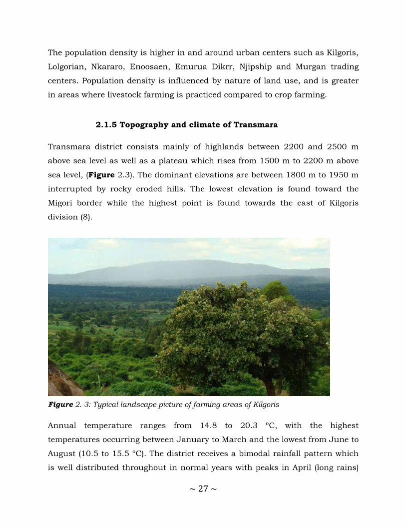
~ 27 ~

The population density is higher in and around urban centers such as Kilgoris,

Lolgorian, Nkararo, Enoosaen, Emurua Dikrr, Njipship and Murgan trading

centers. Population density is influenced by nature of land use, and is greater

in areas where livestock farming is practiced compared to crop farming.

2.1.5 Topography and climate of Transmara

Transmara district consists mainly of highlands between 2200 and 2500 m

above sea level as well as a plateau which rises from 1500 m to 2200 m above

sea level, (Figure 2.3). The dominant elevations are between 1800 m to 1950 m

interrupted by rocky eroded hills. The lowest elevation is found toward the

Migori border while the highest point is found towards the east of Kilgoris

division (8).

Figure 2. 3: Typical landscape picture of farming areas of Kilgoris

Annual temperature ranges from 14.8 to 20.3 ºC, with the highest

temperatures occurring between January to March and the lowest from June to

August (10.5 to 15.5 ºC). The district receives a bimodal rainfall pattern which

is well distributed throughout in normal years with peaks in April (long rains)

~ 28 ~

and December (short rains). Rainfall averages about 1500 mm annually with a

range between a high of 2300 mm and low of 700 mm. Hailstones are

occasionally reported in the west and the highland in the north of the district.

Decline in the total rainfall amount received over the recent years is attributed

to indiscriminate felling of natural vegetation for crop growing, wood fuel and

building materials (8).

The district is suitable for livestock production and arable agriculture.

Currently, the dominant activities include beef livestock rearing and maize

farming. Other enterprises with potential include; dairy farming, quarrying and

mining, sand harvesting, bee keeping and cash crops such as tea. The Maasai

Mara Game Reserve is also an important income generating tourism resource

for the Transmara County Council.

2.1.6 Soil types in Transmara

The two major soil types found in Kilgoris are phaeozems and nitisols.

Phaeozoms are dark colored soils rich in organic matter. The topsoil referred to

as mollic A-horizon is relatively high in organic matter and is non-acid. The

base saturation of the topsoil is over 50%. These soils usually have an ABC

sequence of horizons. The subsoil (B-horizon) usually has a well developed

blocky structure with high porosity. As observed in the area where Chinsaga is

planted, the high level of organic matter confers high natural fertility and an

abundant supply of mineral nutrients. A major disadvantage of these soils is

the high potential for erosion by wind and water if left exposed (9).

Nitisols are the deep, red friable clays observed in some areas. They

accommodate soils more than 150 cm deep. They exhibit clay movement with a

visible shiny red surface throughout the subsoil B-horizon. They have a clay

texture, friable or vey friable and are porous throughout. The chemical

properties of these soils vary widely. The organic matter content, cation

~ 29 ~

exchange capacity (CEC) and percentage base saturation range from low to

high. Nitisols are highly productive soils found in humid tropics with a high

degree of phosphorus sorption. Unlike the phaeozoms, they are quite resistant

to erosion (10).

Regardless of the soil type found in the farming area, the Total Organic Carbon

(TOC) ranges from a low 0.81% to an adequate level of 2.81%. The soil pH

ranges from strongly acid (4.5) to slightly acid (6.65).These areas have an

average altitude of about 2000 m above sea level and fairly cool temperatures

most of the year. The soil is of moderate fertility for growth of maize, cabbage,

tomatoes, spinach and kales among others crops. The soils for production of

Chinsaga in Kilgoris were observed to respond well to nitrogen, phosphorus

and micro nutrient supplementation (9–11).

2.1.7 Growth, maturation and harvesting of Chinsaga

The germination rates of the Chinsaga (Gynandropsis gynandra) seeds are

variable and usually takes about one week to sprout. Plant growth appears

strongest after the first month with an equal increase in auxiliary shoots due to

regular harvest of the apices. This growth of branches is important as it

increases the vegetable foliage. Flowering is often seen towards the end of the

rainy season but may also be triggered by stress. After about two to three

months, the fruits dry releasing seeds into the surrounding ground (12).

~ 30 ~

2.1.8 Objectives

This chapter focuses on documenting the botany and socioeconomics of

Chinsaga cultivation and trade.


These included documentation of:

1. The cultivation of Chinsaga in Kilgoris-Kisii area

2. The distribution and marketing of Chinsaga from Kilgoris

3. The challenges and opportunities experienced in the supply chain of

Chinsaga.

2.2 Methodology

Twelve farms, approximately 300 m apart within Mosocho area of Kilgoris were

purposively sampled. The supply chain was traced from the farmers market in

Mosocho through Kilgoris town to Kisii and eventually to Nairobi. Information

about the activities of the middle-men was obtained from key informants at the

major trading points of Kilgoris, Kisii and Nairobi. Farmers, middle men,

transporters, traders and individuals that purchased from the retail vendors in

the market were also interviewed.

Other interviewees included community leaders and businesswomen that

participate in the Chinsaga trade and supply chain. Semi-structured

discussions directed by the researcher were conducted with a total of 32

participants of all age groups and gender on separate occasions. The responses

~ 31 ~

were collated and thematically analyzed. Research was conducted by a series of

field trips that included collection of qualitative and quantitative data from

December 2007 to July 2008. Plant voucher specimens were collected and

deposited at the Herbarium of the School of Pharmacy, Department of

Pharmacology and Pharmacognosy, University of Nairobi.

2.2.1 Ethical Considerations

Permission for the study was obtained from Kenyatta National Hospital –

University of Nairobi Ethics and Research Committee (KNH-UON

ERC/01/3757). Prior informed consent was also obtained from each

participant and only those who consented to the request and expressed interest

in the research participated in interviews.

2.3 Results

2.3.1 Folklore use of Chinsaga

Through key informant interviews, it was revealed the Abagusii (Kisii people)

recommend the eating of boiled leaves of Chinsaga for treating anemia and by

mothers before and after delivery of a child. Firstly, it was believed to enable

quick recovery from the blood loss experienced during parturition and

secondly, to hasten milk let-down shortly after delivery.

The vegetable is cooked fresh most of the time. When larger quantities are

available, the vegetable is blanched and sundried for preservation. The dried

form is then packed into small bags and may be stored for cooking later.

During preparation, the vegetable is boiled for at least one and a half hours.

Milk, cream or groundnut paste may be added to the second cooking to help

mask the bitter taste often associated with the mature form of the vegetable. In

other situations, it may be mixed with other vegetables such as pumpkin

~ 32 ~

leaves, amaranth or terere. Traditionally, the Abagusii do not blend Chinsaga

with Solanum nigrum (managu) as may be found elsewhere.

2.3.2 Agronomy and commerce of Chinsaga in Kilgoris

It was observed that farming and commercial trade in Chinsaga is widely

practiced in Kisii and Kilgoris town areas during the field study. Chinsaga is

widely consumed by the Kisii. The vegetable is grown in many farms in Kisii

and parts of Kilgoris and large commercial farms are found in leased farms to

the south of Kisii along the Kilgoris-Kisii boundary areas where the population

is less dense.

2.3.3 Sizes of Farms in Kilgoris

The farmers including natives from Kilgoris area who are Maasai and large

number of migrants from Kisii now lease out land and grow the crop. Pieces of

land used for farming ranged from small gardens about an eighth to about one

acre. The most frequent size observed was half an acre, Table 2.1.

Table 2 1: Distribution of land sizes under Chinsaga cultivation in Mosocho area of Kilgoris

Land Size Frequency Proportion%

Less than ¼ acre 2 17 ¼ acre 3 25 ½ acre 6 50 More than ½ acre 1 8

~ 33 ~

2.3.4 Sources of seeds

Many farmers were observed to have a portion of a garden near their houses

used as the seed bank, Figure 2.4. In this garden, the crop is allowed to

mature till it flowers and gives fruits. The pods from these plants are harvested

and dried in the sun. When dry, the pods are rubbed to release the seeds used

for the next crop. The garden also serves as a domestic source of vegetable for

the home during the earlier stages of growth before maturing. In Kenya, seeds

referred to locally as Saget, are available from Kenya Seeds Company. Farmers

also use seeds from their own cultivars. Majority 26 (81%) of the famers

interviewed in Kilgoris reported that they used their own seeds for cultivation of

Chinsaga.

2.3.5 Drivers for commercialization of Chinsaga farming

Based on interviews with key informants, it was established that production

was originally carried out at subsistence level in small gardens. However,

gradual reduction in land sizes, increasing demand in urban centers and

Figure 2. 4: A farmer and his family outside the kitchen house.

~ 34 ~

growing populations away from the rural areas raised the demand to exceed

level of production by subsistence methods.

2.3.6 Soils used to grow Chinsaga

Application of compost mature was important to sustenance of the high

fertility. It was further observed that vegetable farming is practised in the lower

highland extending from Kisii. In the same areas, maize, wheat and pyrethrum

were also grown. On occasion application of micronutrients as foliar fertilizers

was seen to greatly enhance growth of crops.

2.3.7 Stages of growth of Chinsaga

Among the Kisii, Chinsaga is harvested in three distinct phases with the

highest yields occurring in the seventh week. Farmers reported that Chinsaga

requires about four weeks from planting to the first harvest of the tender

sprouts, Figure 2.5. The plants are grown in rows about one foot apart. The

first three harvests served to prune the numbers leaving better spacing

between plants. This first three crop harvests are locally referred to as

Omonyenye. The vegetable at this stage is of mild and gentle taste. The

Omonyenye stage is about four week old crop on a farm. The plants at this

stage will have already undergone the first harvesting during which some

plants are uprooted to allow for optimal spacing. Pruning also allows for the

farmer to select out the poorer plants leaving those that appear to be thriving

better.

Chinsaga two to three months old is described as the Amasabore stage, Figure

2.6. Leaves from the stems and sturdier shoots are harvested weekly. The stage

of the vegetable has a mild acerbic to bitter taste. After the Amasabore stage,

~ 35 ~

the plant begins to flower, and the stage is referred to as Ekegoko, Figure 2.7.

Ekegoko has a bitter taste and is preferred by the older people of the Kisii

community. The vegetable is relished at all stages but preferences are mainly

determined individually. The bitterness of the plant when cooked varies by

variety and appears to be influenced by soil type and the pattern of rain at

different stages of plant growth.

Figure 2. 5: Omonyenye

Figure 2. 6: Amasabore

Figure 2. 7: Ekegoko

~ 36 ~

Overall, well watered crops in fertile soils with plenty of manure will give the

best crop with a moderate level of bitterness palatable to most people. However,

this degree of bitterness is much more in areas with drier hotter and less fertile

soils. The plants will be more stunted and have tougher stalks that make the

vegetable more fibrous to chew. This is probably the least favored form of the

vegetable in diet.

2.4 Production, supply and marketing of Chinsaga

The practice of growing Chinsaga in Kilgoris was introduced by the Kisii since

the Maasai traditionally lived mainly by raising livestock. Upon establishment

of better returns from farming of vegetables, some Maasai have also begun to

take a keen interest in the farming. However, the main traders and consumers

are Kisii and this has helped to retain a fairly controlled supply chain by Kisii

traders.

2.4.1 Chinsaga planting, harvesting and processing

Vegetables production in Kilgoris and Southern Kisii was based on rain fed

system. Single cropping is the most popularly practiced production system.

Farmers growing Chinsaga are the main actors in the supply chain. They

contribute most of the value chain functions. These include ploughing,

planting, soil fertilization, weeding, pest and disease controlling, harvesting

and post harvest handling. The favorable weather conditions make growing

Chinsaga economical and high yielding.

The farms are divided into about 5 portions and planting done at different

times to ensure there was a crop to be harvested at different stages of maturity.

Each section would have a harvest done twice a week giving an average of

about 10 to 15 sacks. The weight of sacks ranged from 12 Kilograms to 22

Kilograms with the mode about 16 Kilograms. Crops grown on a new farm will

~ 37 ~

have good production for two cycles and thereafter the land must be left fallow

or crops changed to have legumes and revert to grazing land for over six

months.

The vegetables are best harvested from the field early in the morning. As the

plants produce a sticky gum as the day progresses and this complicates the

handling while harvesting. Labourers are paid per sack of the crop harvested

by the buyer and the farmer gets money for each sack at a pre-negotiated price

depending on the prevailing market prices. After harvesting, the crop is packed

in gunny bags with an approximate weight of about 18 Kilograms. The

measurement is by visual assessment and by experience.

The market price will vary depending on availability of the vegetable and tends

to be lower in rainy season and higher in the dry season. However, the farmers

have lower pricing power often getting less than optimal returns for their crop

in the markets, Figure 2.8. In addition, they bear a portion of the post-harvest

losses.

Figure 2. 8: Group of farmers waiting for pay by the middle men they supply regularly

Post harvest handling includes sorting, grading, packing, storing,

transportation, loading and unloading. This is done by the farmers or by

traders or brokers. As was observed in many farms, vegetables are sold at the

~ 38 ~

farm. In this case the post-harvesting handling is carried out by the traders or

broker. Most of the farmers, traders or brokers use sacks and ground outside

their residential house. High postharvest losses were observed to occur mainly

as a result of improper harvesting, handling, packaging and poor facilities to

market. A proportion of the Chinsaga gets spoilt before it reaches the market.

2.4.2 Transport of Chinsaga from the farms to markets

It was observed that means of transportation varied widely. Farmers deliver the

vegetables to the producers’ market in the late morning. Predominately

producers use donkeys, Figure 2.9, and motorcycles. Over shorter distances

porters are used, Figure 2.10. Most farmers transported their vegetables to the

nearby market centers such as Mosocho. These market centers may be termed

producers’ markets where farmers negotiate price, traders make purchases and

eventually transport most Chinsaga to urban markets. Vegetable supply is

often spread in heaps on the ground. They are aired by frequently turning the

heap prior to repacking in yellow or green polythene bags.

The producers’ market are more remotely located compared to the more

reknown retailer markets. The retail markets are more accessible in the larger

centers along the main roads. The local county government levies fees on

Chinsaga sale at each level of market, Figure 2.11. Those interviewed felt the

action of levying charges for the growing and supply of these traditional

vegetables was a disincentive by the local government.

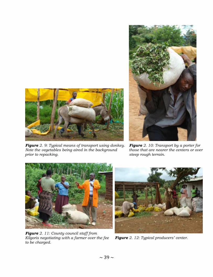
~ 39 ~

Figure 2. 9: Typical means of transport using donkey. Note the vegetables being aired in the background prior to repacking.

Figure 2. 10: Transport by a porter for those that are nearer the centers or over steep rough terrain.

Figure 2. 11: County council staff from Kilgoris negotiating with a farmer over the fee to be charged.

Figure 2. 12: Typical producers’ center.

~ 40 ~

2.4.3 Collection and assembly of Chinsaga from the producers

The collectors or assemblers are the traders in assembly markets who collect

vegetables from farmers in village markets and from farms for the purpose of

reselling it to wholesalers

It was observed that once the vegetables are delivered to the center, they are

removed from the gunny bag and allowed to air, Figure 2.12. This helps to

reduce heating and damage that result from compaction after harvesting and

during transportation. The aired vegetables are then packed into sacks again or

into yellow polythene bags with a capacity of about 10 Kg or into green

polythene bags with a typical capacity ranging from 5-6 Kg. The bags are

punched with holes to allow for aeration and prevent spoilage due to heating

and continued fermentation of the materials.

Figure 2. 13: Commercial vehicle hired to transport Chinsaga at Mosocho market.

Chinsaga is transported to Kilgoris or other towns in Kisii using minivans,

Figure 2.13 from where it is repackaged in smaller bags for onward transport

to larger towns like Nairobi. The market channel identified by observation and

through interviews gave several alternate pathways, Figure 2.14

~ 41 ~

Producers →Consumers Producers → Retailers → Consumers

Producers → Wholesalers → Consumers Producers → Wholesalers → Retailers → Consumers

Producers → Collectors → Retailers → Consumers Producers → Collectors → Wholesalers → Consumers Producers → Collectors → Wholesalers → Retailers → Consumers

Figure 2. 14: Illustration of the Chinsaga market channel

The proportions of each of these components of the market channel for

Chinsaga could not be quantified within the context of this study.

2.4.4 Collection and retailing of Chinsaga

Collectors and retailers are persons that take the role of collecting and retailing

of Chinsaga supplied from the producers’ market. When interviewed

respondents reported that collectors and retailers are expected to be witty and

deeply versed with the knowledge about the producers, their field harvesting

capacities and personalities of each of their suppliers. The collector and

retailers often apply cunning tactics to maximize on their limited finances to

pool together as much supply of Chinsaga as possible. They must know their

niche including where they can obtain large quantities at lower prices and

therefore are important in the Chinsaga value chain. They primarily buy, pool,

sort, repack, transport and supply the wholesale markets.

~ 42 ~

2.4.5 Structure of the supply chain

The brokers and middlemen are important in linking farmers to market and

others in the Chinsaga supply chain. The brokers were observed to exert power

over pricing. They appear to set the price. There were brokers that resided in

Kilgoris and others commuted from Kisii. Most of those from Kisii handled the

market in urban areas. Brokers in the rural areas are important mediators

between the farmers and the urban retailers. Others act on an agency basis on

behalf of urban brokers or retailers.

Brokers are divided into village level brokers, urban brokers and commission

agents. Brokers at village level enable engagement with producers. They are

often focused on getting the best quality in large amounts.

It was observed that there was a small group of traders that bought vegetables

from farmers and collectors in larger quantities and could be termed the

wholesalers. They link many farmers with retailers and consumers. They had

greater capacity for longer storage of the Chinsaga to cover the transit duration

or in the event of glut in supply. Wholesalers often shoulder a portion of the

post harvest losses. The wholesale market is often at Kilgoris and Kisii towns.

They are more capitalized to carry out this storage and transportation. Nearly

all wholesalers are from Kisii town.

At the time of the field visit to Transmara area, Kilgoris was the major center

involved in the supply of the vegetables was determined as Kilgoris town. The

vegetables are packed into sacks or polythene bags at Kilgoris town and loaded

onto small vans (Nissans) and transported to Kisii. Other markets included

Magena and Ogembo on the road to Kisii. Once the vegetables reached Kisii,

they were repacked into smaller packets of about 4 to 6 kilograms. The packets

are then perforated to allow aeration. The packaged material is then loaded

onto buses for transport to markets in Nairobi, Figure 2.15.

~ 43 ~

Figure 2. 15: Distribution of Chinsaga from Kilgoris/Kisii to Nairobi.

The packed vegetables often have designated vendors who receive them in

Nairobi. Once in the city, the first vendors often wholesale to other vendors that

supply the various markets in the city. Others supply clients directly within

offices and homes within the environs of Nairobi reaching as far as Kitengela,

Ngong, Rongai, Ruai and areas along Thika road.

The increase in demand has helped in establishment of commercial viability

and a supply chain that is now almost fully structured. There are fairly well

established farmers, middle men and market suppliers from the growing areas

in Kisii - Kilgoris areas to its main markets in Nairobi and its environs.

The largest part of postharvest management of the vegetables is carried out by

the retailers. They buy and transport the Chinsaga to retail points. They also

grade, displaying and sell the vegetables to consumers. The retailers represent

the final front in the supply as well as value chain. They are important players

in maintaining the consistency of demand that is eventually fed by the

producers.

~ 44 ~

Most retailers buy from wholesalers and focus on supply to urban consumers.

Some retailers buy Chinsaga directly from the farmers but this is less common.

Majority of consumers get their vegetables from the urban retailers who carry

out some additional sorting and cleaning of the vegetables. This helps to

improve the appeal of the vegetables especially by the removal of stiffer stems.

Rural retailers often hold much less stock and have lower turnover compared

to their urban counterparts.

It was noted that consumers of Chinsaga were mainly of three types. The first

type was domestic consumers, who bought Chinsaga for home use. The

domestic consumers were the majority. The second type of consumers

purchased for restaurants and other food outlets. Last were institutional

consumers such as training institutions and schools. These represented the

least mode of consumption.

The majority of clients purchasing the vegetables for restaurants and

institutions had established relationships with the vendors. This loyalty was

common in the supply chain of the Chinsaga. Its role was most often an

important component in guaranteeing supply even during the lean months of

the year. The relationship was also found to play an important part in

protecting the price variations seen seasonally. The regular buyers often got

better bargains. A common practice observed was the addition of vegetables to

the customers as part of this relationship.

Direct purchases by consumers from wholesalers was not observed but may

have happened rarely. Some of the features most sought were consistency of

the heap and its cleanliness. The more tender forms were slightly more popular

and often got finished faster among the retailers.

The major role of value chain actors is to support the market of the Chinsaga

keeping a steady supply and moderation of pricing. The value chain actors help

~ 45 ~

develop the rules of engagement by those in the mainstream trade of Chinsaga.

It was observed that brokers and retailers played the greatest role in setting the

supply and pricing. Much less was observed among the wholesalers. Lack of

formal structures may explain the lack of information and lower price setting

power observed among the farmers. Horizontal linkages of communication were

not clearly in place. Most transactions were cash based indicating low levels of

trust among the players. On the other hand, the retailers often faced the risk of

high losses if they did not sell all the supply within a short time. This tension

between the various market factors often resulted in selling price variations

within the day. Vendors tended to offer vegetables at lower prices towards close

of the day.

Often the purchasers would bargain to get the lowest price possible leaving the

farmers feeling underpriced. The farmers are thus seen as price-takers. In

reaction, farmers were observed to include more stems in the heaps as this

increased the weight and volume of the sack. The purchasers, on the other

hand, desired more leaf hence putting pressure on retailers to cleave off most

of the stems as part of the process of enhancing the appeal of the vegetables to

the consumers. This inadvertently results in substantial changes in volume

and weight of the vegetables with a collated increase in price.

2.5 Discussion and Conclusion

Chinsaga in Transmara is grown as both a subsistence and commercial crop.

The consumption of Chinsaga in urban areas like Nairobi has contributed

immensely to the growing commercial demand for the vegetable. Ambrose- Oji

has attributed the growth of commercial farming of G. gynandra and other

traditional vegetables in Africa to expansion of the middle class especially in

the urban areas (13). The overall effect in Kenya is the increase in the land

utilized for growing the vegetable in Kisii and now on leased land within

Kilgoris as observed during the field visits.

~ 46 ~

The expansion of “supermarket culture” has also driven commercial farming of

Chinsaga. Ngugi et al (14), identifies the integration of traditional vegetable

sales in the supermarket as a major driver of increased demand for indigenous

vegetables. In this study we determined that more families in rural towns have

access to ready packaged traditional vegetables including Chinsaga. Further it

was noted that vegetable vendors are a key source of fresh vegetables for many

homes in the towns. One of the biggest challenges in the trade of the traditional

vegetables include requirement for standardization of product for it to be

acceptable in the international market. Most growers of crops like Chinsaga

would not be prepared to meet these requirements and the supply systems may

not be financially capable of investing to achieve them. Indirectly, international

trade policies may be a barrier to growth of the Chinsaga market(15).

Land availability may be another barrier to expansion of commercial farming of

Chinsaga. Acreage under farming of Chinsaga could be another barrier to

expansion of commercial farming. In this study, most commercial farmers had

half acre dedicated to Chinsaga farming. Other studies in Western Kenya show

that the mean size of land under indigenous crop per farmer has been

continuously decreasing since 1960s(16).

Our interviews revealed that the nature of Chinsaga supply chain is complex.

Actors in the supply chain included farmers, collectors, wholesalers, retailers

and consumers. The typology of the supply chain was however not unique for

Chinsaga and parallels supply chains described for other East African

indigenous vegetables (17).

When inquiries were made to explain the apparent high demand and focus on

supply from Kisii and its environs by clients in the city, key factors were noted.

Most clients in the city believed that Chinsaga from Kisii or Kilgoris were of

superior quality to any other that was brought to the market. There was also a

strong trust system associated with the supply chain. Clients were often keen

~ 47 ~

to know the origins of the vegetables they bought. Upon establishing a trust

relationship with vendors, many would maintain such relationships as their

primary source. Many believed that vegetables from elsewhere grown under

different conditions would not have the same benefits. Similar importance of

loyalty has been described in Costa Rica for supply of indigenous vegetables

(18).

Modern farming has often resulted in monoculture. Traditional vegetables such

as Chinsaga are often grown along with other crops in mixed cultures. This has

the advantage of providing a wider range of crops as sources of food and

doubles up as a strategy that conserves the soil by providing cover throughout

the year reducing soil erosion (19). Observations made in Kilgoris indicate a

trend towards monocultures even for the traditional vegetables on farms that

have been prepared almost purely for commercial goals. The pricing for the

vegetables has reached sufficient levels stimulating specialization by some of

the growers to meet this demand as a mechanism to provide family income.

During the field visits, no use of chemicals was noted. This is a key observation

considering the belief among most consumers is that the production of the

vegetables in Kisii and its environs is largely “organic”. The vegetables are

highly priced as an introductory diet by women shortly after birth in the Kisii

culture. They are also widely believed to be the best vegetable for those that are

unwell. The use of pesticides and fertilizers will greatly alter this property of

purity associated with this source of the vegetable. This may also explain the

low preference for use of the same vegetables from other areas of Kenya or the

environs of Nairobi in the open market. The members of the Kisii community

even in urban areas still preferred to obtain their vegetables from sources they

knew. Other studies in Italy showed that consumers are sensitive to the use of

chemicals in the production of their foods (20).

~ 48 ~

Dixon (21) identified seven factors that strongly compel focus on traditional

vegetables like Chinsaga. Among the seven, include the decline in national food

self-sufficiency resulting from a reduction in agricultural extension support

especially for peasant farming in favor of commercial models using intensive

methods such as green houses. There is also competing needs for the land as

families subdivide pieces into smaller sizes hence larger proportions lost to the

homestead area. In addition, more land is getting consumed to allow urban

infrastructure and real estate development for human settlement.

2.5.1 Conclusion

In conclusion, Chinsaga is cultivated both for subsistence and commerce by

small holder farmers in Kilgoris. It contributes significantly to the livelihood of

families in Kilgoris and parts of Kisii. Chinsaga has positive impacts as a

nutritional and commercial product for communities in Kisii and Transmara

counties, and its demand is increasing in the urban areas. This implies

commercial agriculture of Chinsaga has good prospects; however declining

farm sizes under traditional vegetables may constrain the farming of Chinsaga.

2.5.2 Recommendations

We recommend further surveys to establish proportion of producers carrying

out sorting and grading of vegetables before they are taken to the market as

part of value addition. The survey may help establish the major sources of

losses along the supply chain.

During the field study, no clear formal structures of support were observed. It

would have been expected that training, extension services, farming and

market information, financial services or research should have been made

available considering the importance of the vegetable to the Kisii community.

~ 49 ~

These services would greatly enhance the success of the supply chain for

Chinsaga.

In addition, we recommend that the national and county government adopt

positive planning models that promote production of traditional vegetables

such as Chinsaga. For example, the charging of levies may need to be

addressed if use of traditional foods to combat food insecurity and malnutrition

is to be realized.

2.6 References

1. Johns T, Kokwaro JO. Food plants of the Luo of Siaya district, Kenya. Econ Bot. 1991;45(1):103–13.

2. Chweya JA, Mnzava NA. Cat’s whiskers. Cleome gynandra L. Promoting the conservation and use of underutilized and neglected crops. 11. Institute of Plant Genetics and Crop Plant Research, Gatersleben/International Plant Genetic Resources Institute, Rome, Italy. 54 pp. GaterslebenInternational Plant Genet Resour Inst Rome Italy. 1997;54.

3. Chayamarit K. Cleome gynandra L. Wageningen, Netherlands: Plant Resources of South-East Asia No 8. Vegetables. Pudoc Scientific Publishers; 1993. p. 148–50.

4. Sharma OP. Plant Taxonomy. Tata McGraw-Hill Education; 1993. 504 p.

5. Mishra SS, Moharana SK, Dash MR. Review on Cleome gynandra. Int J Res Pharm Chem. 2011;1(3):681–9.

6. Guarino L. Traditional African Vegetables. Rome Italy Int Plant Genet Resour Inst [Internet]. 1997 [cited 2013 Sep 4]; Available from: http://www2.bioversityinternational.org/publications/Web_version/500/begin.htm

7. Kenya National Bureau of Statistics. Volume 1C Population and housing census

2009 [Internet]. [cited 2014 Jun 22]. Available from: http://www.knbs.or.ke/index.php?option=com_phocadownload&view=category&download=582:volume-1a-population-distribution-by-administrative-units&id=109:population-and-housing-census-2009&Itemid=599

8. Jätzold R, Schmidt H. Farm Management Handbook of Kenya: Natural Conditions and Farm Management Information, Central Kenya:(Rift Valley and Central Provinces)/by Ralph Jaetzold and Helmut Schmidt. Ministry of Agriculture, Kenya; 1983.

~ 50 ~

9. Rachilo JR, Wanjogu SN, Wachira TR. Semi-detailed soil survey of the Olenkasorai (Oyani) area–phase 1 (Kilgoris Division, Narok District). 1988 [cited 2014 Nov 18]; Available from: http://agris.fao.org/agris-search/search.do?recordID=US201300299863

10. Ministry of agriculture, livestock and fisheries state department of agriculture. Soil suitability evaluation for maize production in Kenya [Internet]. GoK; 2014 [cited 2014 May 28]. Available from: http://www.kilimo.go.ke/images/nationalreport_book.pdf

11. Tandi NK, Nyamangara J, Bangira C. Environmental and potential health effects of growing leafy vegetables on soil irrigated using sewage sludge and effluent: a case of Zn and Cu. J Environ Sci Health B. 2004 May;39(3):461–71.

12. Onyango MA, Onyango J. Conservation and seed production of African leafy vegetables at Maseno University botanic garden, Kenya. African Crop Science Conference Proceedings [Internet]. 2005 [cited 2013 Aug 25]. p. 1201–4. Available from: http://www.researchgate.net/publication/230642883_Conservation_and_seed_production_of_African_leafy_vegetables_at_Maseno_University_botanic_garden_Kenya/file/9fcfd5025887c7b72c.pdf

13. Ambrose-Oji B. Urban food systems and African indigenous vegetables: Defining the spaces and places for African indigenous vegetables in urban and peri-urban agriculture. Afr Indig Veg Urban Agric. 2009;1.

14. Tschirley DL, Ayieko MW, Mathenge MW, Weber M. Tegemeo Institute - Where do Consumers in Nairobi Purchase their Food and why does this matter? The Need for Investiment to Improve Kenya’s Traditional Food Marketing System [Internet]. 2004 [cited 2013 Oct 3]. Available from: http://www.tegemeo.org/index.php/research-resources/publications/item/99

15. Dolan C, Humphrey J. Governance and Trade in Fresh Vegetables: The Impact of UK Supermarkets on the African Horticulture Industry. J Dev Stud. 2000;37(2):147–76.

16. Netondo GW, Waswa F, Maina L, Naisiko T, Masayi N, Ngaira JK. Agrobiodiversity endangered by sugarcane farming in Mumias and Nzoia Sugarbelts of Western Kenya. Afr J Environ Sci Technol. 2010;4(7):437–45.

17. Weinberger K, Pasquini M, Kasambula P, Abukutsa-Onyango M. 11 Supply Chains for Indigenous Vegetables in Urban and Peri-urban Areas of Uganda and Kenya. Veg Prod Mark Afr Socio-Econ Res. 2011;169.

18. Sáenz-Segura F. Contract farming in Costa Rica: opportunities for smallholders? [Internet]. Wageningen University; 2006 [cited 2014 Jun 22]. Available from: http://library.wur.nl/WebQuery/wda/1805409

19. Chweya J. Potential for agronomic improvement of indigenous plant Germplasm in African agriculture. A case study of indigenous vegetables in Kenya.

~ 51 ~

Safeguarding Genet Basis Afr Tradit Crops CTA NetherlandsIPGRI Rome. 1994;105–10.

20. Boccaletti S, Nardella M. Consumer willingness to pay for pesticide-free fresh fruit and vegetables in Italy. Int Food Agribus Manag Rev. 2000;3(3):297–310.

21. Dixon J, Omwega AM, Friel S, Burns C, Donati K, Carlisle R. The Health Equity Dimensions of Urban Food Systems. J Urban Health. 2007 May 1;84(1):118–29.

~ 52 ~

CHAPTER THREE

3.0 Phytochemical and chromatographic fingerprint of Gynandropsis gynandra

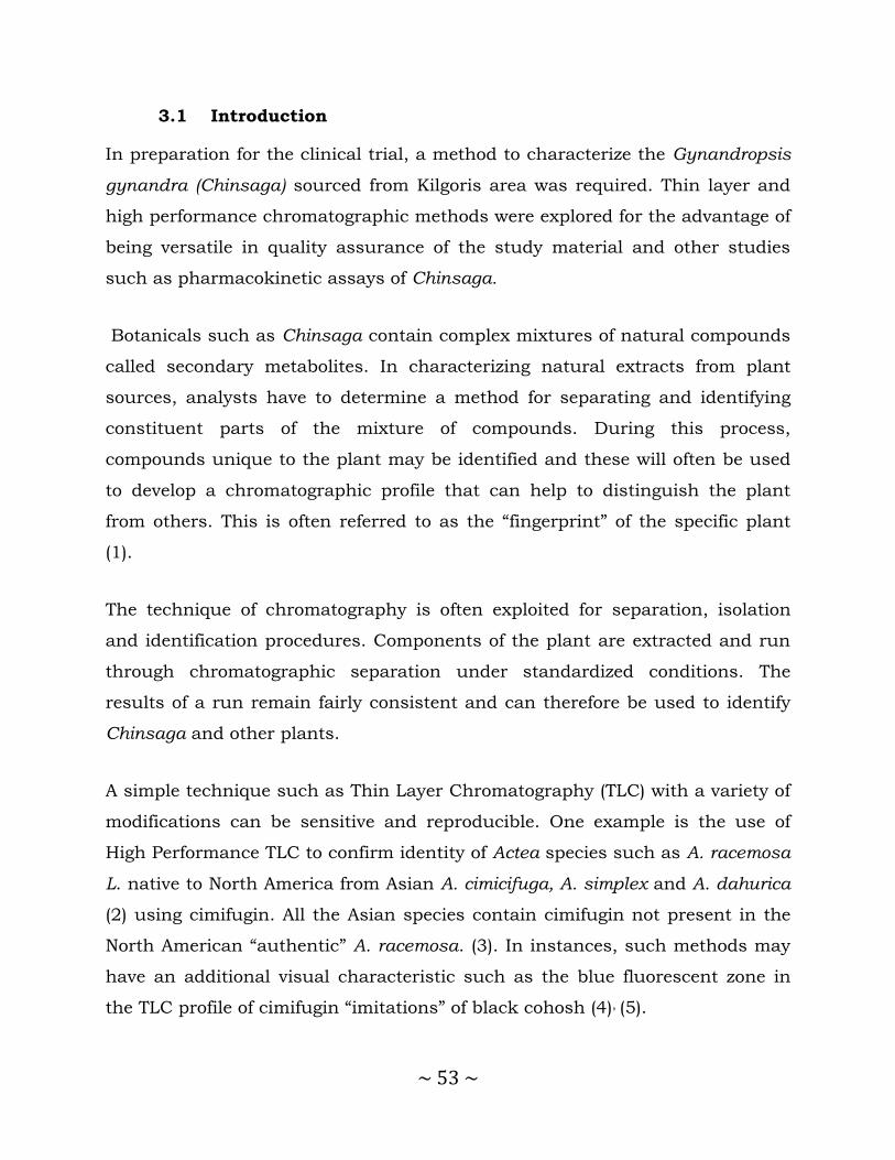
~ 53 ~

3.1 Introduction

In preparation for the clinical trial, a method to characterize the Gynandropsis

gynandra (Chinsaga) sourced from Kilgoris area was required. Thin layer and

high performance chromatographic methods were explored for the advantage of

being versatile in quality assurance of the study material and other studies

such as pharmacokinetic assays of Chinsaga.

Botanicals such as Chinsaga contain complex mixtures of natural compounds

called secondary metabolites. In characterizing natural extracts from plant

sources, analysts have to determine a method for separating and identifying

constituent parts of the mixture of compounds. During this process,

compounds unique to the plant may be identified and these will often be used

to develop a chromatographic profile that can help to distinguish the plant

from others. This is often referred to as the “fingerprint” of the specific plant

(1).

The technique of chromatography is often exploited for separation, isolation

and identification procedures. Components of the plant are extracted and run

through chromatographic separation under standardized conditions. The

results of a run remain fairly consistent and can therefore be used to identify

Chinsaga and other plants.

A simple technique such as Thin Layer Chromatography (TLC) with a variety of

modifications can be sensitive and reproducible. One example is the use of

High Performance TLC to confirm identity of Actea species such as A. racemosa

L. native to North America from Asian A. cimicifuga, A. simplex and A. dahurica

(2) using cimifugin. All the Asian species contain cimifugin not present in the

North American “authentic” A. racemosa. (3). In instances, such methods may

have an additional visual characteristic such as the blue fluorescent zone in

the TLC profile of cimifugin “imitations” of black cohosh (4), (5).

~ 54 ~

TLC also has additional applications in current Good Manufacturing Practices

(cGMP) regulations for botanicals in which identity testing for raw materials is

required as a safety precaution. Chromatographic profiling may also

distinguish closely related herbs. Plants are classified primarily along family,

genus and species. Each family of plants is further subdivided into genera

(plural of genus). Members of a genus (species) share many anatomical and

phytochemical characteristics differentiating them from other genera in the

same family. The phytochemical components present in a plant can be used to

characteristerise plants used as herbal medicines.

Phytochemical fingerprinting has been demonstrated to be a powerful

technique for the quality control of herbal medicines (6). A phytochemical

fingerprint is a unique pattern that indicates the presence of multiple chemical

markers within a sample. The quantity of a chemical marker can be an

indicator of the quality of a herbal medicine.

The European Medicines Agency (EMEA) defines chemical markers as

chemically defined constituents or groups of constituents of a herbal medicinal

product which are of interest for quality control purposes regardless whether

they possess any therapeutic activity (6). Ideally, chemical markers should be

unique components that contribute to the therapeutic effects of a herbal

medicine. As only a small number of chemical compounds have clear

pharmacological actions, other chemical components are also used as markers

(7).

The EMEA categorizes chemical markers into analytical markers and active

markers. Analytical markers are the constituents or groups of constituents that

serve solely for analytical purposes, whereas active markers are the

constituents or groups of constituents that contribute to therapeutic activities.

~ 55 ~

There are other classifications of chemical markers. For example, Srinivasan (8)

proposed the following four categories: active principles, active markers,

analytical markers and negative markers. Active principles possess known

clinical activities; active markers contribute to clinical efficacy; analytical

markers have no clinical or pharmacological activities; and negative markers

demonstrate allergenic or toxic properties. All markers may contribute to the

evaluation, standardization and safety assessment of herbal medicines.

Visualization in Thin Layer chromatography (TLC) is simplified for colored

components such as flavanoids and carotenoids but other components require

additional techniques. Chromatographic results (fingerprint profile) can provide

a powerful tool for monitoring plant extracts (9).

3.2 Objectives

The main objective of this study was to develop a fingerprintTLC and HPLC

chromatogram of Gynandropsis gynandra which can be used for qualitative

and quantitative purposes.

The specific objectives were to:

1. Develop a method of extraction of Chinsaga

2. Develop a TLC fingerprint of Chinsaga

3. Develop a finger print HPLC profile of the extract of Chinsaga

4. Compare the HPLC profile of Chinsaga at various stages of maturity.

~ 56 ~

3.2.1 Review of the phytochemistry of Chinsaga

Several compounds have been isolated from Chinsaga (Gynandropsis

gynandra). These include chromones, flavones, flavonols, lipids, oxazolidines,

steroids, sulfur compounds and triterpenes. Table 3.1 is a summary of the

chemical components obtained from a search on the NAPRALERT database

which can be found at: http://napralert.org/.

Table 3 1: Compounds isolated from Gynandropsis gynandra (Capparidaceae)

Compound Compound Class Reference

Cleomin Oxazolidine (10)

Sitosterol,Beta: Steroid (11)

Chromone,5-7-Dihydroxy Chromone (12)

Luteolin Flavone (13)

Centaureidin Flavonol (13)

Flavone,5-Hydroxy-3-4'-7-Trimethoxy Flavonol (13)

Kaempferol Flavonol (13)

Kaempferol-3-O-Beta-D-Glucosyl-Glucoside Flavonol

(13)

Myricitrin Flavonol (13)

Quercitrin Flavonol (13)

Rutin Flavonol (13)

Glucobrassicin Sulphur compounds (14)

Glucobrassicin,Neo Sulphur compounds (14)

Glucocapparin Sulphur compounds (14)

Glucoiberin Sulphur compounds (14)

Thiocyanate,Iso: Methyl Sulphur compounds (14)

Amyrin,Beta Triterpenes (15)

Amyrin,Alpha Triterpenes (15)

Cleogynol Triterpenes (15)

Lupeol Triterpenes (15)

Taraxasterol Triterpenes (15)

http://napralert.org/

~ 57 ~

Nine lipids have been isolated from Chinsaga including; Arachidic Acid, Capric

Acid, Lauric Acid, Linoleic Acid, Myristic Acid, Oleic Acid, Palmitic Acid,

Palmitoleic Acid and , Stearic Acid (16).

3.3 Materials and Methods

3.3.1 Procurement and preparation of the Chinsaga and Kale

Approximately 660 Kg (80 bags) of Chinsaga was bought in June 2009 from the

commercial centers located in the farming areas of Kilgoris, about 230 Km west

of Nairobi City. Chinsaga was transported to Kisii High School where the

vegetables were sorted out to remove extraneous materials and excess stems

after which they were washed to remove soil and dust. The washed vegetable

was allowed to drip to reduce wetness before loading into the large cooking

pots. The vegetable was steamed without addition of water for one hour with

regular checking to avoid charring. Charring adversely affects the flavor of the

whole cooking rendering the vegetable bitter and unpalatable.

After steaming, the material was then transported in pots to Nyankoba tea

factory 23 Km from Kisii for spreading and drying on beds. In the tea factory,

the vegetables were blown with warm air and turned regularly till they attained

near crisp dryness. This pre-drying stage was critical to preserve the material

during transportation to Nairobi to the School of Pharmacy where it was dried

further till completely crisp with an average moisture reduction of about 94%

compared to the raw material. The dried material was then packed into well

aired porous polyester sacks which had been washed and dried. It was later

emptied into and milled using a hammer mill (Makiga, Kariobangi, Kenya) at

the School of Pharmacy. The powdered material was packed into a single sack

with a total weight of about 62 kilograms.

Kale (Sukuma wiki), (1200 kg) for use in the study was purchased from the

local market in Kisii. The vegetables were transported to Kisii School kitchen

~ 58 ~

where they were cooked and partially dried before transportation to the tea

factory for further drying. The pre-dried material was also transported to

Nairobi and dried till crisp. The dried material was milled and sent for

packaging at the same site as the Chinsaga.

3.3.2 Packaging of the milled dried Chinsaga and Kale

Sachets were identified as the most feasible and reasonably priced packing

material. The sachets were also aesthetically appealing and easy to use. The

dried milled Chinsaga would also receive adequate protection from elements in

the environment during an estimated 12 months expected for use in the study

when stored at room temperature. Each sachet (Figure 3.1) had an average

weight of 9 grams equivalent to 180 grams of the cooked wet material.

Figure 3 1: Sample Sachet of powdered vegetables

A serving on a regular eating plate averages between 150 to about 250 grams

arrived at after making servings of the cooked material on typical plates used to

serve food. Packing was done at Bespack Foods Company located in Nairobi

and regularly contracted by other food industries to package food products.

~ 59 ~

3.3.3 Extraction and analytical profile using chromatography

3.3.3.1 Materials

Analytical grade triethanolamine (BDH Laboratory Supplies, Poole, England),

anhydrous sodium acetate (Fluka Chemie GmbH, Buchs, Switzerland),

ammonium acetate (Loba Chemie PVT. Ltd) and glacial acetic acid (Sigma-

Aldrich Laborchemikalein GmbH, Seelze, Germany) were used during method

development. Methanol (Fischer Scientific U.K. Ltd.) and acetonitrile (VWR

International Ltd., Poole, England) used in preparation of all chromatography

mobile phases were of HPLC grade.

All aqueous solutions used in the study were prepared using purified water

obtained through reverse osmosis treatment and ultra filtration through

successive 0.45 µm and 0.2 µm membrane filters using a combined Arium

61316 RO and Arium 611 VF water system (Sartorius AG, Göttingen,

Germany).

3.3.3.2 Extraction of Chinsaga

Dried ground material was used for development of phytochemical and

chromatographic profile of Chinsaga. Working standard solution was prepared

by accurately weighing 17.58g and sequentially extracting to exhaustion a

sample of milled Chinsaga with chloroform and 70% ethanol. The milled

powder was weighed and loaded into a silk pouch. The pouch was tied to seal

the opening and placed in a glass bottle into which solvent for extraction was

added. The bottle was then placed in the sonication bath, run for 15 minutes

and drained to recover the extract. Divided portions of the fresh solvent was

added and the extraction procedure repeated until there was no detectable

change in readings for extract obtained as measured using UV at the 220

nm.This procedure was carried out for both solvents. Chloroform and 70%

ethanol extracts were combined to give a single Chinsaga extract (Figure 3.2)

~ 60 ~

which was reduced to using a rotary evaporator (Buchi Labortechnik AG, Flawil

Switzerland)

Figure 3 2 Extraction of milled dried Chinsaga

The thick gummy residue obtained by re-dissolving and combining the

chloroform and 70% ethanol extracts (Chinsaga extract) was then used to carry

out solubility tests.

3.3.4 Assessment of solubility

Solubility of the Chinsaga extract was tested by applying a drop on a white

ceramic plate placed at a slight tilt. A drop of solvent at a time was then

applied to a location just above it on the slant and allowed to wash down

through the extract spot. An ideal universal solvent for the extract was

identified by the extent of wash achieved. In testing for solubility using

solvation in a vial, a small amount of the Chinsaga extract was loaded at the

~ 61 ~

bottom of a vial and small amounts of solvent added with intermittent

sonication.

Solvent was added in 0.5 ml portions till there was no observable change in the

material that remains insoluble at which point it is presumed no further

solvation is taking place. Visual assessment was made on the volume of

material that remains and this was used to gauge the best solvent of mixture of

solvents to use. This was vital to ensure safety even for chromatographic

columns

3.4 Chromatographic profiling of Chinsaga extract

3.4.1 High Performance Liquid chromatography (LC)

instrumentation

The LC apparatus consisted of a Merck Hitachi LaChrom HPLC System (Hitachi

Ltd, Tokyo, Japan) incorporating the following components: a quaternary low

pressure gradient pump model L7100, a variable wavelength UV detector model

L7400, a variable injection volume autosampler model L7200 supported by

Merck-Hitachi Model D-7000 Chromatography data station software - HSM

Manager Version 4.1 (Merck KGaA, Darmstadt, Germany and Hitachi

Instruments Inc., San Jose, USA). Mobile phase preparations were degassed by

Organic modifier and sonication of the general mobile phase preparation using

a Sonorex Super RK103H ultrasonic bath (Bandelin Electronic, Berlin,

Germany) for 15 min. The variable injection volume auto sampler allowed

sample solutions to be injected into the chromatographic system without using

a sample loop of fixed volume. This facilitates variation in volume of injected

sample without having to replace the loop physically.

The chromatography column was a reversed-phase Phenomenex Gemini-NX®

C18 column of dimensions 250 mm length and 4.6 mm internal diameter with

particle size 5µm and pore size 110Å (Phenomenex, Torrance, California, USA).

~ 62 ~

The temperature was controlled using a thermostatically controlled Clifton

unstirred water bath (Nickel-Electro Ltd., Weston-S-Mare, Somerset, England).

Mobile phases were pumped at a constant flow rate of 1.5 mL/min throughout

method development. Column back pressures were maintained below 200 bar.

The upper limit was set at 250 bar.

The wavelength for use in analysis was established by carrying out a spectral

run from 200nm to 700 nm against a neat solution of 70% ethanol for

background correction. Regions of λ maxima and λ minima absorption were

established.

3.4.2 Working standard solution of Chinsaga extract

A 70% ethanol in water was selected as the solvent of choice. The

concentrations of the analyte compounds were calculated in terms of the

weight of dry material (g)/total volume of extract (ml). The combined chloroform

and 70% ethanol extract (Chinsaga extract) constituted the primary standard

used to generate other concentrations.

3.4.3 Mobile phase composition

The different mobile phases prepared during method development comprised

varying the proportions of water, acetonitrile, methanol, propan-2-ol and formic

acid. In some cases ammonium acetate at different pH values was also tested

to determine the effects of pH on separation. Mobile phases were prepared by

mixing appropriate volumes of the salts solutions with water before adjusting

pH to the desired value using the molar equivalent solution of the parent acid

or buffer salt.

The volume of propan-2–ol, methanol or acetonitrile required to yield the

desired proportions of the different mobile phase components was achieved

~ 63 ~

using programming available in the Merck Hitachi HPLC system equipped with

a four channel solvent inlet solenoid valve control. All solutions were degassed

with an ultra-sonic water bath prior to use (Table 3.2).

Table 3 2: Solvents used as mobile phase in developing of a fingerprint

chromatogram of Chinsaga

Component Composition

A Acetonitrile 50% in water B Methanol 50% in water

C Formic Acid 0.4% in water

The first mobile phase consisted of a mixture made using A: B: C, (Table 3.2),

in the ratios 80: 10: 10. (% v/v). Working standard solution (20 µL) was

injected into the LC system.

3.5 Results

3.5.1 Extraction of cooked Chinsaga

Dried milled material weighing 17.58g was sequentially extracted to exhaustion

using chloroform and 70% ethanol. Extraction with chloroform yielded 1.53 g

(8.7%) while 70% Ethanol gave 1.08 g (6.1 %). The two were combined to give a

single extract

3.5.2 Assessment of solubility

The best solubility for the Chinsaga extract was achieved with 70% ethanol and

the lowest solubility was seen in ethyl acetate and 50% methanol. Acetone,

acetonitrile, acetonitrile with 1-3% formic acid, 50% acetonitrile in water and

methanol gave intermediate solubility (Table 3.3).

~ 64 ~

Table 3 3: Solubility of the water extract of milled Chinsaga

Solvent

Observations Conclusion

(Solubility)

Acetone Very good washing away of the green matter and leaves slightly less of the grey mass.

Fair

Acetonitrile It dissolves small components of the green constituent leaving a

green cake like friable matter at the bottom of the vial. It appears

to overlap with methanol. The prominent whitish cake like mass is either dissolved or is masked by the green undissolved pigment.

Fair

Acetonitrile

50% in

Water

Appears to dissolve most materials well and sends the undissolved

matter into a very fine suspension. It dissolves most of the matter.

Fair

Acetonitrile

with 1-3%

Formic

acid

Similar wash to acetonitrile with a brownish residue remaining in

suspension.

Fair

Ethanol Dissolves the green matter and white precipitate at the bottom

very well but still has a refractive portion of green near the walls of

the vial.

Good

Ethanol

70-80%

Very good solution of all materials. The whole extract is suspended

including the white matter and no refractive precipitate is noted

on the bottom edges of the vial.

Very good

Ethyl acetate

Good solution of the green color and matter but leaves behind the grey mass similar to methanol.

Poor

Methanol Dissolves all matter except for a refractive white cake that comes

off the bottom of the vial. No further solution occurs even on

warming. Addition of equal volume of water (1.0 ml) only serves to make the solution more cloudy but dissolves the white precipitate.

Addition of more methanol (0.5 ml) does not change the

cloudiness and still leaves a greener color precipitate compared to

70-80% ethanol solution

Fair

Methanol

50%

Poor solution of the materials. Most remains in the residue Poor

Water Able to dissolve all the other matter except the green pigment.

This remains as a distinct particle that appears unlikely to

dissolve despite addition of more solvent. The resultant solution has a pale orange brown color.

Fair

~ 65 ~

3.5.3 TLC profile of Chinsaga extract

A solution of the Chinsaga extract was spotted onto a normal phase silica

coated plate and run using 100% Hexane. No spot was observed in the

development of the plate. Using ethyl acetate, a single red colored spot at an Rf

of 0.8 visible at UV 320 nm was observed. A mixture of ethyl acetate: methanol:

water in the ratios of 50:20:10, yielded the highest separation visible to the

naked eye and UV light (Figure 3.3).

Figure 3 3: TLC of the 70% ethanol extract developed on normal phase silica plate using ethyl acetate: methanol: water in the ratio of 50:20:10.

3.5.4 Spectral analysis of ethanolic solution of Chinsaga

extract

An absorbance λ maxima was identified at about 255nm and was used in

method development.

~ 66 ~

3.6 Optimization of fingerprint HPLC fingerprint

chromatogram

3.6.1 Effects of organic modifiers on separation of components

Using the mixture of acetonitrile 50% in water (A), methanol 50% in water (B),

formic Acid 0.4% in water (C), here referred to as A: B: C (Table 3.2) in the

ratios 80: 10: 10. (% v/v) as mobile phase, a working standard solution (20 µL)

was injected into the LC system. Very poor separation of the analyte

compounds was achieved (Figure 3.4), with no distinct peak and almost all

components eluting close to the solvent front.

In the next step, the proportion of the organic phases was reduced to give a

composition (A:B:C) of 75:15:10. In this run, there was partial separation of

some of the peaks from the solvent front. There appeared to be first four

probable bands as indicated in the Figure 3.4 showing the effects of reducing

the amount of acetonitrile and increasing the ratio of methanol. The ratio A:B:C

of 65:30:5 % v/v resulted in greater tailing of components probably part of the

solvent front. The four peaks initially separated were reduced to two. It was not

clear if they merged or eluted among the wash out in the tailing from the

solvent front Figure 3.4. The addition of methanol was seen to cause merging

of the peaks and increase tailing.

To confirm this, the ratio of methanol was reduced and that of acetonitrile

increased, Figure 3.4d, to give a mixture in the ratio A: B: C of 40:20: 40 (%

v/v). The result was clearer separation of the first three peaks within four

minutes but there appeared tailing effect persistent till the end of the first few

minutes overlapping with about two other peaks eluting after four minutes

Figure 3.4(d). Initial adjustments in components of the mobile phase targeted

only variation of the organic modifiers.

~ 67 ~

Chromatogram Mobile phase

a

2.642.84, Pea

k 13.64 4.14

4.80 5.25 6.73 7.77 10.07 10.73 13.55 15.05 18.19 20.94 23.17

0 2 4 6 8 10 12 14 16 18 20 22 24

Retention Time (min)

0.0

0.2

0.4

0.6

0.8

1.0

1.2

1.4

Intensity (AU)

Ratio of mobile phase(A:B:C)

80: 10: 10

b

2.13 2.212.35

3.00, Peak 1

3.18 3.433.98

5.42 5.91 7.38 9.40 13.61 21.05

0 2 4 6 8 10 12 14 16 18 20 22 24 26 28


0.0

0.2

0.4

0.6

0.8

1.0

1.2

1.4

Intensity (AU)

75:15:10

c

2.122.31

2.67 3.30, Peak 1

4.04 4.81 5.40 5.88 6.75 7.25 8.82 9.41 10.35 11.90

0 1 2 3 4 5 6 7 8 9 10 11 12 13


0.0

0.2

0.4

0.6

0.8

1.0

1.2

1.4

Intensity (AU)

65:30:5

d

1.912.66

3.704.26 4.89 5.19 6.02 14.51

0 2 4 6 8 10 12 14 16 18 20 22 24 26


0.0

0.5

1.0

1.5

2.0

Intensity (AU)

Ratio of

(A:B:C)40:20

: 40

40:20:40

Figure 3 4: Effect of methanol on separation of ethanolic extract of Chinsaga

3.6.2 Effects of pH on separation

The pH of the solution was also changed in the subsequent injections (series),

Figure 3.5, by addition of ammonium acetate to a pH of 4.07. This had very

little effect in the chromatogram but may have slightly reduced the extent of

tailing of the components from the solvent front as indicated in the

chromatogram Figure 3.5(a) using a Phenomenex Gemini-NX 5 µm Column,

temperature of 40 ˚C, Mobile phase components: A: methanol (50%), B:

acetonitrile (50%), C: formic acid (0.4%) adjusted to pH 4.07 using 0.02 mM

~ 68 ~

ammonium acetate. Mixture made of the ratio of A: B: C of 80: 10: 10 (% v/v).

Flow rate: 1.20 mL/min. Detection: 255 nm. Injection volume: 10 µL.


a

1.982.67

3.704.27 4.92 5.21

0 2 4 6 8 10 12 14 16


0.0

0.5

1.0

1.5

2.0

Intensity (AU)

pH 4.07

b

0.52

1.81 2.03

2.66

3.46, Peak 1

3.96 4.56 4.80

0 1 2 3 4 5 6 7


0.0

0.5

1.0

1.5

2.0

Intensity (AU)

pH 6.7

c

1.802.02

2.663.40, Pe

ak 13.87 4.46

0 2 4 6 8 10 12 14 16 18


0.0

0.5

1.0

1.5

2.0

Intensity (AU)

pH 7.48

Figure 3 5: Effect of pH on separation of 70% ethanol extract of Chinsaga

The pH of the solution was further raised to 6.7, Figure 3.5 and Figure 3.6,

using a solution of 0.02 M ammonium acetate. There appeared to a greater

reduction in the tailing effect observed earlier and the peaks had a better

separation profile as shown in the chromatogram (a). Further work was done

replacing formic acid 0.4% solution with 20mM ammonium acetate solution

adjusted to a pH of 6.7. The changes observed were not significant as indicated

in the Figure 3.5 (b).

The pH was finally raised to 7.48 and the chromatogram obtained showed only

a slight reduction in elution time especially for the third peak but the general

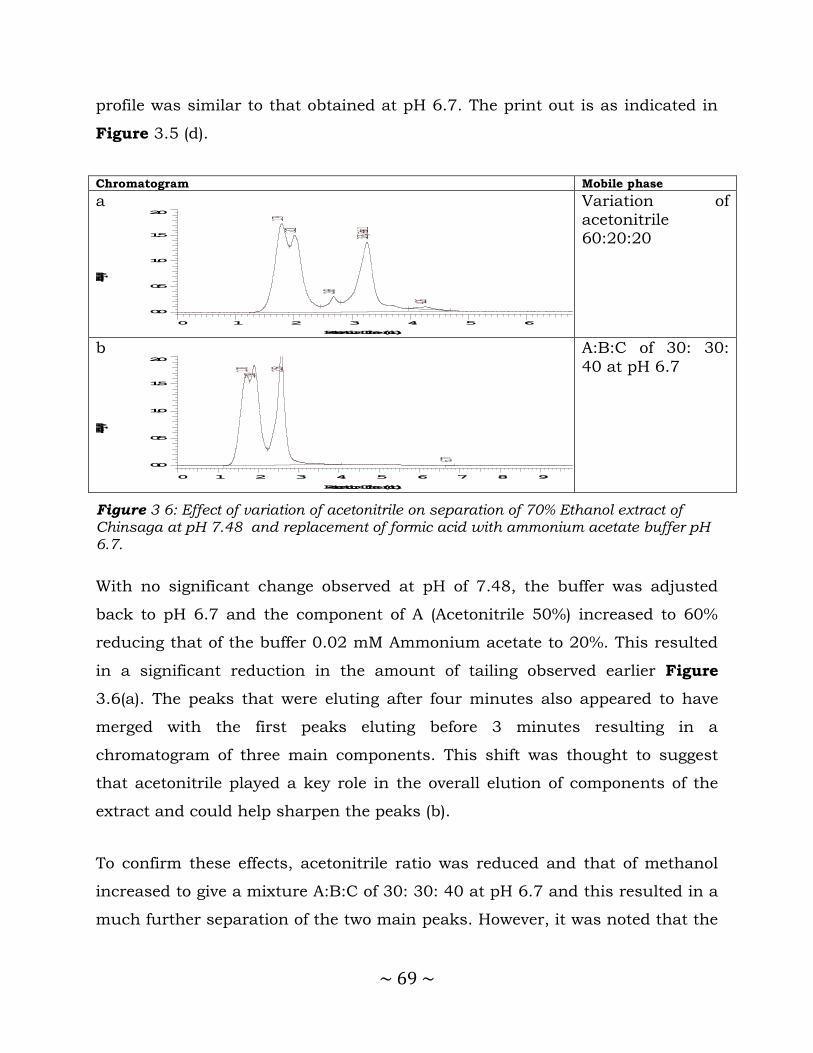
~ 69 ~

profile was similar to that obtained at pH 6.7. The print out is as indicated in

Figure 3.5 (d).


a

1.792.01

2.68

3.26, Peak 1

4.26

0 1 2 3 4 5 6


0.0

0.5

1.0

1.5

2.0

Intensity (AU)

Variation of acetonitrile 60:20:20

b

1.70 1.90 2.58

6.77

0 1 2 3 4 5 6 7 8 9


0.0

0.5

1.0

1.5

2.0

Intensity (AU)

A:B:C of 30: 30:

40 at pH 6.7

Figure 3 6: Effect of variation of acetonitrile on separation of 70% Ethanol extract of Chinsaga at pH 7.48 and replacement of formic acid with ammonium acetate buffer pH 6.7.

With no significant change observed at pH of 7.48, the buffer was adjusted

back to pH 6.7 and the component of A (Acetonitrile 50%) increased to 60%

reducing that of the buffer 0.02 mM Ammonium acetate to 20%. This resulted

in a significant reduction in the amount of tailing observed earlier Figure

3.6(a). The peaks that were eluting after four minutes also appeared to have

merged with the first peaks eluting before 3 minutes resulting in a

chromatogram of three main components. This shift was thought to suggest

that acetonitrile played a key role in the overall elution of components of the

extract and could help sharpen the peaks (b).

To confirm these effects, acetonitrile ratio was reduced and that of methanol

increased to give a mixture A:B:C of 30: 30: 40 at pH 6.7 and this resulted in a

much further separation of the two main peaks. However, it was noted that the

~ 70 ~

two main peaks each also appeared to consist of two unresolved components

as seen in the Figure 3.7.

1.842.05

2.74

3.42, Peak 1

4.674.87

6.89 7.34 7.94

0 1 2 3 4 5 6 7 8 9 10 11 12 13


0.0

0.5

1.0

1.5

2.0

Intensity (AU)

Figure 3 7: Effect of increasing methanol to acetonitrile ratio on separation of Chinsaga ethanolic extract.

3.6.3 Simplification of mobile phase components

To minimize the complexity in preparation of mobile phase, effort was made to

explore the effects of only adjusting organic modifier components while

maintaining a simple solution of formic acid. The mobile phase was run with

the components: A: methanol (50%), B: acetonitrile (50%), C: formic acid (0.4%)

adjusted to pH 6.7 using 0.02 mM ammonium acetate. Mobile phase mixture

made of the ratio of A:B:C of 40: 20: 40 (% v/v). Flow rate: 1.20 mL/min.

Detection: 255 nm. Injection volume: 10 µL, Figure 3.8 (a).

To understand the contribution of methanol, a run was made in which the

methanol component was eliminated altogether giving a mixture consisting of A

(Acetonitrile 50%) and C (Formic acid 0.4%) in the ratio 40: 60 % v/v. The

chromatogram obtained, Figure 3.8 (b) indicated that there was better peak

shape however the tailing effect on the solvent front was seen to have

increased.

The second peak was however much sharper and clearer than obtained

previously. Following this observation, effort was made to replace methanol in

subsequent trials with other organic modifiers to improve the separation.

~ 71 ~


a

1.872.60

4.044.55 5.31 5.61 15.98 20.13 30.63

0 5 10 15 20 25 30 35


0.0

0.5

1.0

1.5

2.0

Intensity (AU)

A: methanol (50%), B: Acetonitrile (50%), C: Formic acid (0.4%) adjusted to pH 6.7 using

0.02 mM Ammonium acetate. Mixture made of the ratio of A:B:C of 40: 20: 40 (% v/v)

b

1.802.46

3.26 3.44, Peak 1

3.805.06

6.13 7.43 8.19

0 2 4 6 8 10 12 14 16 18 20 22 24 26 28


0.0

0.5

1.0

1.5

2.0

Intensity (AU)

A(Acetonitrile 50%) and C(Formic acid 0.4%) in the ratio 40: 60 % v/v

Figure 3 8: Effect of acetonitrile and methanol based mobile phase mixtures on separation of ethanolic extract of Chinsaga.

3.6.4 Effects of propan-2-ol on separation

A solution of propan-2-ol was added to the mobile phase to give a mixture

consisting of acetonitrile: propan-2-ol : water of (11: 1 : 10) as component A

and the solution of Formic acid 0.4% was run as B in the ratio (A:B) of 65:35 %

v/v. The result was an increased separation of the early peaks as indicated in

the chromatogram in Figure 3.9.

The addition of propan-2-ol appears to have improved separation of

components at the solvent front. To investigate this effect further, the

composition of A was varied to from A: acetonitrile: propan-2-ol: water (75: 13:

62), B: formic acid (0.4%) pH 2.3. Mixture made of the ratio of A:B of 35: 65 (%

v/v) which was a reversal of the previous ratio. The result showed an

improvement in the separation of early components in the chromatogram (a).

A further increase in the composition of propan-2-ol in the mobile phase was

made to give a mixture in A: acetonitrile: propan-2-ol: water of 75: 50: 25 and

B: formic acid (0.4%) pH 2.3 run in the ratio A:B of 35:65.

~ 72 ~


a

1.69 1.90 1.972.25

2.52 2.643.47, P

eak 13.93

5.89

7.20 9.01 9.67

0 2 4 6 8 10 12 14 16 18 20 22 24


0.0

0.1

0.2

0.3

0.4

0.5

Intensity (AU)

A: Acetonitrile: Propan-2-ol: Water (75: 13: 62), B: Formic acid (0.4%) pH 2.3. Mixture made of the

ratio of A:B of 35: 65 (% v/v)

b

1.70 1.90 1.972.26 2.51 2.65

3.48, Peak 1

4.14

6.45

7.86 10.27 10.89

0 2 4 6 8 10 12 14


0.0

0.1

0.2

0.3

0.4

0.5

Intensity (AU)

A: Acetonitrile: Propan-2-ol: Water of 75: 50: 25 and B: Formic acid (0.4%) pH 2.3 run in the

ratio A:B of 35:65

Figure 3 9: Effect of propan-2-ol of separation of ethanolic extract of Chinsaga

The result showed an increased merging of the solutes and loss of the initial

separation. It suggested that increase in propan-2-ol in the mobile phase would

reduce the separation of the components as seen in chromatogram (b).

3.6.5 Effect of gradient elution on separation

The change in elution time and improved resolution in the early components

suggested that effort could be made to explore using a gradient approach to

separate elements eluting below five minutes. A mobile phase consisting of a

gradient was run as shown in the Table 3.10.

Table 3.4 is a summary of the mobile phase program used in the development

of the chromatographic method for the Chinsaga extract on column:

Phenomenex Gemini-NX 5 µm. Column temperature: 40 ˚C. Mobile phase

components: A: Acetonitrile: Propan-2-ol: Water (70:50:25), B: Formic acid

(0.4%) pH 2.3. Mixture made of the ratio of A:B of 35: 65 then 20:80 (% v/v).

Flow rate: 1.20 mL/min. Detection: 255 nm. Injection volume: 10 µL.

~ 73 ~

Table 3 4: Mobile phase program used for components: A: Acetonitrile: Propan-2-

ol: Water (70:50:25) in the development of a chromatographic profile of Chinsaga

extract.

Injection (Series) 71 Injection (Series) 76

Time A (%) Time A (%)

0 5 0 2

10 25 5 5

12 25 10 15

15 5 15 30

20 5 16 35

20 2

The chromatographic outcome was as shown in Figure 3.10.

Chromatogram A% in Mobile phase

2.022.38 2.4

23.15 4.01 5.21 5.94 7.57 8.19 9.82 11.01 12.13 13.69 15.54 17.09

19.0120.01 25.75 28.19 35.56 38.71

0 5 10 15 20 25 30 35


0.0

0.1

0.2

0.3

0.4

0.5

Intensity (AU)

2.13 2.49 2.59 4.62 6.90 8.71 9.95 11.16 11.73 12.27 12.71 13.53 14.13 15.09 16.43

18.0619.19

0 5 10 15 20 25 30


0.0

0.1

0.2

0.3

0.4

0.5

Intensity (AU)

Figure 3 10: Effect of gradient elution on separation of ethanolic extract of Chinsaga. Series refers to the electronic serial record of the injection of the sample.

There was improved resolution in the components of the extract and this was

the first time components were not concentrated at the solvent front. This was

the most important phase in the development of the method and gave

indication that good resolution could be achieved by using a gradient of

~ 74 ~

solvents in the method. Subsequent efforts were made to refine it. Some of the

tested alterations were as indicated in 3.11.

Chromatogram A% in Mobile phase 2.13 2.49 2.59 4.62 6.90 8.71 9.95 11.16 11.73 12.27 12.71 13.53 14.13 15.09 16.43

18.0619.19

0 5 10 15 20 25 30


0.0

0.1

0.2

0.3

0.4

0.5

Intensity (AU)

2.05 3.01 6.03 7.45 11.01 11.3912.03

12.67 13.15 13.59 13.95 14.63 15.21 16.15 16.95 17.63 18.23

20.13

21.790 2 4 6 8 10 12 14 16 18 20 22 24 26


0.0

0.1

0.2

0.3

0.4

0.5

Intensity (AU)

1.95 3.07 5.19 6.28

8.01 8.97

10.32 11.01 11.74 12.83 14.32

16.48

18.55

0 2 4 6 8 10 12 14 16 18 20 22 24 26 28


0.0

0.1

0.2

0.3

0.4

0.5

Intensity (AU)

1.96 3.08 5.045.89

6.69 7.568.27

8.87 9.83 10.80 11.83 12.63 13.46

18.25

20.18

0 2 4 6 8 10 12 14 16 18 20 22 24 26 28


-0.05

0.00

0.05

0.10

0.15

0.20

Intensity (AU)

Figure 3 11: Effect of gradient program variation on separation of components of ethanolic extract of Chinsaga.

After maximizing the separation of components under the fixed ratio of

70:50:25, slight variations in this composition were introduced and effects

analysed. In the first instance, the ratio of acetonitrile was increased from 70 to

75 in method series 101. The chromatogram appeared to have better peak

sharpness (Figure 3.12). Components eluting between 5 to 10 minutes

~ 75 ~

appeared more clearly separated and an area between 12 and 16 minutes had

a set of poorly separated compounds. However, there was some distinction

achieved for compound close to the peaks eluting just after 21 minutes.

Method series 101 1.86 2.16

2.97 4.01 4.59 5.586.20

6.67 7.067.33

8.028.63 8.92 9.20 9.81 11.16 12.37 12.75 13.11 13.31 13.52 14.29 14.49 15.04 16.51 17.13 19.53 20.02

21.8622.33 23.42

0 2 4 6 8 10 12 14 16 18 20 22 24 26


0.0

0.1

0.2

0.3

0.4

0.5

Intensity (AU)

Figure 3 12: Optimized separation of components of ethanolic extract of Chinsaga.

Mobile phase: A: Acetonitrile: Propan-2-ol: Water (75:50:25), B: Formic acid

(0.4%) pH 2.3. Mixture made of the ratio of A:B of 35: 65 then 20:80 (% v/v).

Flow rate: 1.20 mL/min. Detection: 254nm.

3.6.6 Improving peak sharpness

To increase peak sharpness, an addition of acetonitrile and reduction in

propan-2-ol was made from 75:50:25 (101) to 85:35:25 (102) and the effects

were as shown in Figure 3.13. The mobile phase components were: A:

acetonitrile: propan-2-ol: water (70:50:25), B: formic acid (0.4%) pH 2.3 with a

mixture made of the ratio of A:B of 35: 65 then 20:80 (% v/v) and a flow rate of

1.2ml/min.

~ 76 ~


1.86 2.16

2.97 4.01 4.595.58

6.206.67 7.06

7.338.02

8.63 8.92 9.20 9.81 11.16 12.37 12.75 13.11 13.31 13.52 14.29 14.49 15.04 16.51 17.13 19.53 20.02

21.8622.33 23.42

0 2 4 6 8 10 12 14 16 18 20 22 24 26


0.0

0.1

0.2

0.3

0.4

0.5

Intensity (AU)

1.90 2.19

2.55 3.07 4.35 4.915.74

6.366.80 7.

197.45

8.128.73 9.02 9.26 9.79 10.81 11.57 12.01 12.45 12.85 13.11 14.29 14.95 15.75 16.42 17.36 17.83 19.42 19.99

21.8722.34 23.44

23.87

0 5 10 15 20 25 30


0.0

0.1

0.2

0.3

0.4

0.5

Intensity (AU)

2.01 2.18 2.42 3.16, Peak 1

3.72 5.215.82

6.396.87 7.

277.48

7.83 8.52 9.82 10.33 11.35 12.07 12.82 13.22 13.43 13.83 14.15 14.63 15.62 15.87

18.2218.91 20.92 21.87 25.51 26.79

0 5 10 15 20 25 30


0.0

0.1

0.2

0.3

0.4

0.5

Intensity (AU)

Figure 3 13: Optimization of peak resolution of ethanolic extract of Chinsaga.

The changes in chromatogram series 106 suggested some increased separation

of the components between 5 and 10 minutes, better sharpening of peaks

between 11 and 16 minutes and some increase in resolution between the key

peak at 21 minutes and those that follow at 21.6 and 22.8.

Achieving any further separation would now be very difficult without increasing

the run time and application of other detection strategies such as diode array

or Mass spectroscopy to help resolve peak purities. Refinement of the method

using a newer column and the gradient only needed slight tuning to improve

peak resolutions from Chromatogram series 122 to 157 using A: acetonitrile:

~ 77 ~

propan-2-ol: water (85:35:25), B: formic acid (0.4%) pH 2.3, fllow rate of 1.20

mL/min, detection at 255 nm and injection volume of 20 µL. This is shown in

the Figure 3.14.


1.70 1.802.06

2.69 3.02, Peak 1

3.574.72

6.26 6.888.02

8.60 9.16 10.23 10.76 11.17 11.54 12.23 12.55 12.79 13.07 13.25 13.49 13.67 14.06 14.51 14.87 15.63 16.37 17.32

18.0318.67 21.00 21.95 23.19 24.95 25.92 26.58

0 5 10 15 20 25 30


0.0

0.1

0.2

0.3

0.4

0.5

Intensity (AU)

1.69 1.812.11

2.182.91,

Peak 13.58

5.085.42 5.72 6.17

6.356.73 7.48 7.94 8.52 9.62 10.16 10.77 11.67 11.93 12.55 13.94 14.35 14.92 15.59 15.87 16.28 17.13 17.30 17.60 18.11

18.5918.94 19.55

19.88 21.99 22.86

0 2 4 6 8 10 12 14 16 18 20 22 24


0.0

0.1

0.2

0.3

0.4

0.5

Intensity (AU)

1.68 1.772.09

3.04 3.44, Peak 1

5.075.79

6.507.05 7.73 8.50 8.87 9.20 9.43 9.76 9.87 10.04 10.17 10.37 10.61 10.8

4 11.04 11.67 11.94 12.63 12.89 13.15 13.6014.13

14.54 15.1715.65 15.95 16.31 16.54 17.21

0 2 4 6 8 10 12 14 16 18 20


0.0

0.1

0.2

0.3

0.4

0.5

Intensity (AU)

Figure 3 14: Optimized separation of ethanolic extract of Chinsaga components.

It was noted that the peak at 5 minutes in 152 appeared to have a hump at the

peak front that would require further testing to resolve if it was an artifact or as

a result of an overlap with another component.

~ 78 ~

3.6.7 Chromatography of different stages of Chinsaga

maturity

The method developed to this point was then applied for use to compare the

three stages of the plant (Omonyenye, Amasabore and Ekegoko) and to see if

there was any significant difference in the ratios of the resolved peaks.

Extracts were obtained using 70% ethanol in water and run to compare the

chromatographic profiles. The results showed no visible differences in pattern

under these conditions Column: Phenomenex Gemini-NX 5 µm, Column

temperature: 40 ˚C, Mobile phase components: A: acetonitrile: propan-2-ol:

water (85:35:25), B: formic acid (0.4%) pH 2.3, Flow rate: 1.20 mL/m). The

chromatogram for Omonyenye, Amasabore and Ekegoko was as illustrated in

Figure 3.15.


1.68 1.772.09

3.04 3.44, Peak 1

5.075.79

6.507.05 7.73 8.50 8.87 9.20 9.43 9.76 9.87 10.04 10.17 10.37 10.61 10.8

4 11.04 11.67 11.94 12.63 12.89 13.15 13.6014.13

14.54 15.1715.65 15.95 16.31 16.54 17.21

0 2 4 6 8 10 12 14 16 18 20


0.0

0.1

0.2

0.3

0.4

0.5

Intensity (AU)

Figure 3 15: Chromatogram of different stages of Chinsaga 70% Ethanol extract.

~ 79 ~

3.7 Discussion and Conclusion

A chromatographic method for HPLC fingerprint analysis was designed,

developed and optimized for dried milled Chinsaga. The method can be used to

identify Gynandropsis gynandra. During the processing of the study materials,

it was observed that the materials lost averagely 93% weight during the drying

step. Other studies suggest 83.3 to 86.6 %. Other components found in

Chinsaga include 4.8% protein g, 0.4% fat, 5.2% carbohydrate and 1.2 % fiber.

Mineral composition was claimed to be Ca 288 mg, P 111 mg, Fe 6.0 mg,

ascorbic acid 13 mg (16–18).

During this study, chloroform followed by 70% ethanol in water was

established as the optimal solvent system. Investigation of plant materials has

been done using different solvents or mixtures to obtain optimal yields. In

other instances, serial extraction may be applied from the least polar to the

polar solvents and later combined. The goal is to obtain the highest extractive

rate of all possible components of interest such as extraction of high-priced

compounds from vineyard and wine byproducts from grape seeds and skins

(19).

Extraction of phenolic compounds from vine shoots using superheated liquid

extraction (SHLE), microwave-assisted extraction (MAE), and ultrasound-

assisted extraction (USAE) were compared. Use of 80% (v/v) aqueous ethanol

at pH 3; 180 °C, and 60 min for SHLE; 140 W and 5 min microwave irradiation

for MAE; and 280 W, 50% duty cycle, and 7.5 min extraction for USAE yielded

the best values. SHLE reported better extraction efficiencies compared to the

other approaches(19).

However, ethanol is not always the most optimal solvent for extraction hence

the process of determination of the best mix involving others such as methanol

(5). In the case of hesperidin, an abundant bioflavonoid in Penggan (Citrus

~ 80 ~

reticulata) peel, with various pharmacological properties was extracted best

using ultrasonic extraction with methanol (20).

Chromatographic profile of ethanol extracts has been used for differentiating

closely related plant species. Fabiana species (Solanaceae family) extracts have

long been used in Argentinean traditional medicine as anti-inflammatory,

antiseptic, bone fractures and others diseases. Aqueous and ethanolic extracts

of four Fabiana species (Fabiana bryoides Phil., Fabiana punensis A.C. Arroyo,

Fabiana densa J. Rèmy and Fabiana patagonica Speg.) were compared by

HPLC. It was observed they had different phytochemical patterns, which also

showed different potencies in biological activities when tested (21).

The development of the extraction and chromatographic method was adopted

from similar applications used for quality control for plant extracts and applied

in differentiating botanical species by High Performance Chromatography

(HPLC) (22).

Guided by the solubility observed, 70% ethanol was chosen as the best

compared to the other solvents tested. The goal was to ensure that solvents

and equipment used would be those that may be readily available in settings

where use of the procedure may be adopted as a standard method in quality

assurance or quality control technique at a commercial scale (23).

The mobile phase and chromatographic column Phenomenex Gemini-NX 5 µm

was selected for use in the development of the HPLC method since it is widely

used and available in analytical laboratories. The column has a wide pH

stability range between pH 1 to 12. In this column, ethyl bridges are used to

connect vicinal free silanol groups improving resilience to chemical challenge at

the pH extremes compared to ordinary C18 columns (24).

~ 81 ~

Given the wide range of chemical components expected in a typical plant

extract, it was also ideal for the separation of constituents of the plant and

giving sharp peaks (22). Multiple peaks were observed in the chromatogram of

the extract of Chinsaga.

Similarly, the detection wavelength used in the development process was fixed

at 255 nm since at this wavelength most compounds would be visible. Another

consideration made in selecting this wavelength was to allow the method

developed to be successfully applied using HPLC instrumentation equipped

with fixed wavelength UV detectors, typically set at 254 nm (25), without any

need for further adjustments if adopted as a national standard method.

The principle in establishing a suitable mixture of solvents for the mobile phase

was compatibility to UV and mass spectrometry detectors. This narrowed the

options to propan-2-ol, acetonitrile and other volatile buffers based on

ammonium or acetate (26). It was also important that they should be fairly

easy to obtain locally.

3.7.1 Conclusion

In conclusion, using the solubility profile, a mobile phase composed of

acetonitrile, propan-2-ol, water and formic acid was formulated. The separation

of extract components showed propan-2-ol was the most suitable combination

with acetonitrile improving peak shapes compared to those based on methanol.

The extract from the Chinsaga used in this study showed poor solubility in

pure solvents. A graded series of chloroform followed by 70% ethanol was

established as the most optimal method. A solution of 70% Ethanol achieved

the best solubility profile for the extract. A finger print HPLC chromatogram the

extract of dried milled Chinsaga was developed to compare similar materials

and serve as a method of determining similarities of other Chinsaga samples.

~ 82 ~

3.7.2 Recommendation

The recommendations from this study would include application of the method

developed in the assessment of Chinsaga as part of the food analysis protocols

at the Kenya Bureau of standards. Both the method and fingerprint

chromatogram can be refined as a Chinsaga standard locally. The method can

also be useful in assaying during pharmacokinetic studies of Chinsaga.

3.7.3 Study Limitations

Identity of peaks will require a mass spectrometer or use of standards along

with the analysis. The lack of a MS and the standards limits the identification

of the major components in the fingerprint chromatogram.

3.8 References

1. Reich E, Schibli A. High-performance thin-layer chromatography for the analysis of medicinal plants [Internet]. Thieme; 2007 [cited 2013 Sep 8]. Available from: http://books.google.com/books?hl=en&lr=&id=arvZGnebybwC&oi=fnd&pg=PP13&dq=Reich,+E.+Schibli,+A.+High-Performance+Thin-Layer+Chromatography+for+Analysis+of+Medicinal+++Plants.&ots=yQHmyZSNC7&sig=OOhIAvYnxArg8JR6YCXTKnq8ZIo

2. He K, Pauli GF, Zheng B, Wang H, Bai N, Peng T, et al. < i> Cimicifuga</i> species identification by high performance liquid chromatography–photodiode array/mass spectrometric/evaporative light scattering detection for quality control of black cohosh products. J Chromatogr A. 2006;1112(1):241–54.

3. Compton JA et al. Reclassification of Actaea to include Cimicifuga and Souliea (Ranunculaceae): phylogeny inferred from morphology. Taxon. 1998;47:593–634.

4. Ankli A, Reich E, Steiner M. Rapid High-Performance Thin-Layer Chromatographic Method for Detection of 5 Adulteration of Black Cohosh with Cimicifuga foetida, C. heracleifolia, C. dahurica, or C. americana. J AOAC Int. 2008;91(6):1257–64.

5. Rai A. The Antiinflammatory and Antiarthritic Properties of Ethanol Extract of Hedera helix. Indian J Pharm Sci. 2013;75(1):99.

~ 83 ~

6. Biomarkers Definitions Working Group. Biomarkers and surrogate endpoints: preferred definitions and conceptual framework. Clin Pharmacol Ther. 2001 Mar;69(3):89–95.

7. Jain KK. The handbook of biomarkers [Internet]. Springer; 2010 [cited 2013 Sep 8]. Available from: http://books.google.com/books?hl=en&lr=&id=Tr6JEXqSWk0C&oi=fnd&pg=PR5&dq=K.K.+Jain,+The+Handbook+of+Biomarkers&ots=BOwhbKPvrO&sig=rV_YNqsAAQ4nmER4H-w8eee010w

8. Srinivasan VS. Challenges and scientific issues in the standardization of botanicals and their preparations. United States Pharmacopeia’s dietary supplement verification program—A public health program. Life Sci. 2006;78(18):2039–43.

9. Biological Fingerprinting of Herbal Samples by Means of Liquid Chromatography [Internet]. [cited 2013 Jun 16]. Available from: http://www.hindawi.com/journals/cri/2012/532418/

10. Jain AC, Gupta SM. Minor phenolic components of the seeds of Gynandropsis gynandra. J Nat Prod. 1985;48(2):332–3.

11. Ramiah N, Nair AG. Chemical investigation of the leaves of Gynandropsis gynandra. J Med Plants. 1983;4(1):411–2.

12. Purification and characterisation of polyphenol oxidase from leaves of Cleome gynandra L. [Internet]. [cited 2013 Jun 15]. Available from: http://www.sciencedirect.com/science/article/pii/S0308814611007655

13. Anbazhagi T, Kadavul K, Suguna G, Petrus AJA. Studies on pharmacognostical and in vitro antioxidant potential of Cleome gynandra Linn. leaves. Nat Prod Radian. 2009;8(2):151–7.

14. Mrsna RN, Smnrenusnan D. CHEMICAL EXAMINATION OF THE SEEDS OF CLEOME PENTAPHYLLA LINN. PART I: ISOLATION OF OLEOMIN. 1937 [cited 2013 Sep 2]; Available from: http://202.41.82.144/rawdataupload/upload/insa/INSA_1/20005b8f_45.pdf

15. Das PC, Patra A, Mandal S, Mallick B, Das A, Chatterjee A. Cleogynol, a Novel Dammarane Triterpenoid from Cleome g ynandra. J Nat Prod. 1999;62(4):616–8.

16. Chweya JA, Mnzava NA. Cat’s whiskers, Cleome gynandra L. [Internet]. Bioversity International; 1997 [cited 2013 Sep 4]. Available from: http://books.google.com/books?hl=en&lr=&id=ZE6Sis0BVx4C&oi=fnd&pg=PA4&dq=Chweya,+J.A.+%26+Mnzava,+N.A.,+1997.+Cat%E2%80%99s+whiskers.+Cleome+gynandra+L.+Promoting+the+conservation+and+use+of+underutilized+and+neglected+crops&ots=rIexbtD-ms&sig=s8q3NmSJGDGA7ZTTDOmCE27rCcg

17. Guarino L. Traditional African Vegetables. Rome Italy Int Plant Genet Resour Inst [Internet]. 1997 [cited 2013 Sep 4]; Available from:

~ 84 ~

http://www2.bioversityinternational.org/publications/Web_version/500/begin.htm

18. Mnzava NM, Dearing JA, Guarino L, Chweya JA, de Koeijer H. Neglected Leafy Green Vegetables Crops in Africa [Internet]. Bioversity International; 1999 [cited 2013 Aug 25]. Available from: http://books.google.com/books?hl=en&lr=&id=nseTAusJEDMC&oi=fnd&pg=PP7&dq=Ethnobotany+of+traditional+leafy+vegetables+in+kenya&ots=FnXAwoPjLw&sig=kGK9xpfghKnpR4xc4zMrwll8Qfw

19. Delgado-Torre MP, Ferreiro-Vera C, Priego-Capote F, Pérez-Juan PM, Luque de Castro MD. Comparison of Accelerated Methods for the Extraction of Phenolic Compounds from Different Vine-Shoot Cultivars. J Agric Food Chem. 2012 Mar 28;60(12):3051–60.

20. Ma Y, Ye X, Hao Y, Xu G, Xu G, Liu D. Ultrasound-assisted extraction of hesperidin from Penggan (Citrus reticulata) peel. Ultrason Sonochem. 2008 Mar;15(3):227–32.

21. Cuello S, Alberto MR, Zampini IC, Ordoñez RM, Isla MI. Comparative study of antioxidant and anti-inflammatory activities and genotoxicity of alcoholic and aqueous extracts of four Fabiana species that grow in mountainous area of Argentina. J Ethnopharmacol. 2011 Sep 1;137(1):512–22.

22. Li S, Han Q, Qiao C, Song J, Cheng CL, Xu H. Chemical markers for the quality control of herbal medicines: an overview. Chin Med. 2008;3(1):7.

23. Liang Y-Z, Xie P, Chan K. Quality control of herbal medicines. J Chromatogr B. 2004;812(1):53–70.

24. Wu N, Dempsey J, Yehl PM, Dovletoglou A, Ellison D, Wyvratt J. Practical aspects of fast HPLC separations for pharmaceutical process development using monolithic columns. Anal Chim Acta. 2004;523(2):149–56.

25. Swartz M. HPLC detectors: a brief review. J Liq Chromatogr Relat Technol. 2010;33(9-12):1130–50.

26. Sasidharan S, Chen Y, Saravanan D, Sundram KM, Latha LY. Extraction, isolation and characterization of bioactive compounds from plants’ extracts. Afr J Tradit Complement Altern Med [Internet]. 2011 [cited 2014 Sep 3];8(1). Available from: http://www.ajol.info/index.php/ajtcam/article/view/60483

~ 85 ~

CHAPTER FOUR

4.0 Baseline Nutrition and Demographic

Characteristics of Study Participants in the Chinsaga

Clinical Trial

~ 86 ~

4.0 Background

In this chapter we report on the demographic data, nutrition practices and

breast feeding that may potentially relate to lactational and hematological

outcomes among postnatal mothers enrolled into the Chinsaga clinical trial at

Kenyatta National Hospital.

Worldwide, about 800 women die daily due to pregnancy related causes (1).

Nearly all occur in developing countries and more than half are sub-Saharan

Africa. The majority of deaths happen around the time of delivery. Recent

national surveys in Kenya have estimated that approximately 6500 women die

from childbirth-related causes each year (450–500 deaths per 100 000 live

births)(1). Factors associated with high maternal mortality are maternal

nutritional status, age, parity, education and marital status (2).

The city of Nairobi is faced with inadequate housing, supply of clean and safe

water, sanitation and heavy reliance on food supplies from rural areas.

Concurrently, reduction in agricultural productivity in areas within and near

the city renders about 47% of the population food-insecure (3). Most of such

households spend about three-quarters of their income on food. Like in many

other cities in Africa, food is usually available but about a third of households

may not attain a nutritionally adequate diet due to cost. Anemia and vitamin A

deficiencies are prevalent among children and women (3). The value of fruits

and vegetables is associated with better health outcomes and reduced risk of

diseases.

Frequency of consumption of fresh fruits and vegetables is high in Kenya.

Markets serve as the main supply of fresh fruits and vegetables and about

three quarters of rural households grow some for sale (4). Access to fresh fruits

and vegetables is a global challenge. While WHO/FAO recommend 400g daily,

it has not been fully achieved (5). In Nairobi, consumption is highly correlated

~ 87 ~

with wealth status. Most fruits and vegetables exhibit seasonality in

availability. In addition, local markets in rural areas are more restricted in the

variety of fruits and vegetables available for purchase. The Table 4.1 adapted

from Ayieko et al summarizes some of the fresh fruits and vegetables consumed

by households in Nairobi (6).

Table 4 1: Weighted Household Purchases of Major Fresh Fruits and Vegetables in Nairobi. Monthly purchases of fruits and vegetables (Adapted from Ayieko et al (5).

Item % of

Households

purchasing

Mean(Kg) Average monthly expenditure

(Ksh)

Tomatoes 96% 9.8 229

Onions 94% 4.5 114

Sukuma wiki (Kales) 82% 12.7 99

Cabbage 77% 3.8 68

Irish potatoes 77% 22.7 144

Carrots 67% 5.0 61

Cooking bananas 35% 13.3 48

Sweet potatoes 24% 6.7 23

French beans 16% 3.9 13

Average total monthly purchases of vegetables over all households is Ksh 779

Item % of

Households

purchasing

Mean(Kg) Average monthly expenditure

(Ksh)

Bananas 77% 9.1 146

Oranges 74% 4.2 112

Mangoes 53% 5.4 65

Avocado 48% 5.1 45

Pawpaw 40% 10.7 64

Average total monthly purchases of fruits over all households (Ksh) 431

4.1.1 Breastfeeding and its role in reproductive health

The ability of breastfeeding to delay return of fertility is well known. (7,8). In

1988, the Bellagio Consensus Conference proposed guidelines promoting the

use of lactational amenorrhea method (LAM) for family planning. In the

practice of LAM, the woman fully or nearly fully breastfeeding remain

amenorrhaic the first 6 months postpartum. Cumulative 6-month life-table

pregnancy rate as low as 0·45% has been demonstrated among women who

~ 88 ~

relied on LAM as their only family planning method (one woman pregnant in

month 6). Other advantages include high acceptance and efficacy, viability,

ease of initiation and safely as a starting method for breastfeeding women (9).

The over 98 % efficacy of LAM has been widely demonstrated and results

suggest possible utility beyond 6 months. It is highly effective as an

introductory postpartum method in a variety of cultures, health care settings,

socioeconomic strata, and industrial and developing country settings (10–12).

Other studies have been carried out to determine correlating factors to success

or failure of LAM. In one study maternal nutritional status was assessed to

play an independent role in the return of ovulation after delivery (13). Mothers

in urban settings may also experience differences in effectiveness of LAM and

experience lower efficacy (14).

4.1.2 Main objective

The purpose of this study was to establish the baseline characterstics of the

study participants in relation to; demographic data, behavior related to

nutrition and breast feeding in mothers recruited into the Chinsaga clinical

trial at Kenyatta National Hospital.

4.1.3 Specific Objectives

Specific objectives were to:

1. Describe the nutritional practices with regard to intake of fruits,

vegetables and animal products;

2. Identify foods eaten by lactating mothers that are believed to increase

milk output;

~ 89 ~

3. Measure the prevalence of pica habit and use of herbs that are believed

to promote lactation.

4.1.4 Study justification

It has been observed that many women have beliefs that guide what they can

eat during pregnancy and/or breast-feeding. Some are based on folklore

associated with eating some types of food. It is still possible that some of the

myths may not support improvements in nutritional outcomes.(15). This study

was designed to identify poor nutrition practices that may be related to

postnatal hematological and lactational outcomes. This will help in the design

of interventions to promote good postnatal nutrition.


4.2.1 Ethical considerations

The study was conducted with approval from Kenyatta National Hospital –


ERC/01/3757) and the Kenyatta National Hospital clinical services

department. Only code numbers were used in the records of the participants.

No names and identifiers were used in the files. Informed consent was obtained

from all participants and confidentiality maintained by use of codes instead of

patients’ names. Primary and secondary data was safely stored in a locked

cupboard and a password protected computer accessible only to the study

investigator.

4.2.2 Study Design and location

This assessment of the baseline characteristics as a cross sectional study

carried out as part of the randomized placebo controlled triple blind study. The

~ 90 ~

study was carried out at Kenyatta National Hospital. The hospital is the largest

teaching and referral hospital in Kenya serving mainly women from Nairobi and

its environs.

4.2.3 Study duration and time frame

This study was conducted over a period of four months between August and

November 2008 enrolling mothers who met the inclusion criteria.

4.2.4 Participant’s inclusion criteria:

Patients were included if they met the following criteria:

1. Women below 35 years of age and in their seventh to eighth month of current pregnancy attending KNH postnatal clinic

2. Healthy (free from chronic disease with exception of asymptomatic HIV positive mothers)

3. Not smoking

4. Not been on Chinsaga 4 weeks prior to enrolment

5. Willing to consent to participate in the study

6. Available for the 28 days follow-up period within Nairobi or its environs.

4.2.5 Participant’s exclusion criteria:

Patients were excluded if they:

1. Were smokers

2. Were instructed not to breastfeed for any reason

3. Had a chronic diseases such as inflammatory diseases (rheumatoid

arthritis, Crohn's disease, colitis ulcerosa), diabetes, asthma and hypertension.

4. Used prescription medication or nonsteroidal anti-inflammatory drugs on

a regular basis

5. Used of vitamin or non iron mineral supplements for the last 1 month

6. Used corticosteroid treatment and immunostimulators for the last 4 wks.

7. Had hemoglobin concentration below 8g/dL

~ 91 ~

4.2.6 Sample size considerations

The overall aim was to determine if Chinsaga is biologically active or inactive in

altering iron metabolism in lactating women shortly after delivery using

surrogate makers as endpoints. The baseline characteristics of the participants

in the Chinsaga clinical trial study involved all 119 mothers as described in

this chapter. Effect estimations are described in chapters 5 and 6.

4.2.7 Recruitment procedures

Figure 4 1: Flow diagram of recruitment process at Kenyatta National Hospital clinic 17 for Chinsaga study.

The Figure 4.1 indicates the steps of the recruitment process to enrolment of

volunteers at clinic 18 of Kenyatta National Hospital. Mothers who attended

~ 92 ~

and anticipated delivering at the Maternal Child Health (MCH) clinic 18 were

informed about the study by nurse officers at the clinic. The potential

volunteers would then be directed to the recruitment officer and asked if they

are interested in taking part in the study. Those that accepted to join the study

were screened for eligibility by checking through the inclusion and exclusion

criteria Figure 4.2.

Figure 4 2 Consort diagram for enrollement of study volunteers into kale (control) and Chinsaga (Treatment) arms at KNH at visit one (days 0).

Those that qualified for recruitment were adequately informed of the study and

again asked if they still wished to join the study. Additionally, they would be

asked if any more information was needed for them to make an informed

decision to participate. Those that agreed to join the study were required to give

informed and documented consent. They were allowed to make this decision at

another visit if unable to do so on the first day .

4.2.8 Case definition of Pica habit

Pica habit was defined as regular consumption of one of the following: stone,

soil, soap or any other non-food materials. Poor nutrition practices is

consumption of fruits and vegetables less than once a week, meat less than

once a week, of foods rich in calcium and low consumption of iron rich foods.

4.2.9 Data collection

Volunteers were asked to complete a questionnaire which was designed to

obtain information on lactation beliefs and nutritional habits (Appendix 3). In

~ 93 ~

addition, information on demographic characteristics such as sex and age were

obtained. The volunteers were required to complete the questionnaire in the

premises of the clinic where they were encouraged to seek help for sections

they did not understand. Since the focus of the study was on food intake rather

than portion sizes for nutrient calculations, the food frequency questionnaire

(FFQ) was used to obtain information on the type and frequency of foods

consumed by study volunteers in the preceding 7 days. Various foods from

different food groups were read out to the respondent, who in return was

required to state the number of times she had consumed this food within the

past week.

4.2.10 Data Management

All data was entered into an Excel spread sheet within 24 hours of data

collection. The data was regularly checked for inconsistencies. When identified,

the researchers reviewed patient records and interviewed patients on

subsequent visits to reconcile the inconsistencies. The data was backed up

every week and copies kept at a separate site. All patient identifying

information was kept under lock and key by the principal investigator. All data

was password protected.

4.2.11 Data analysis

The key outcomes of interest were the pica habit, frequency of breastfeeding,

maternal beliefs and poor maternal nutritional practices. Since the study was

mainly cross sectional, most of the analysis was restricted to descriptive data

analysis. Continuous variables were summarized as the median and inter-

quartile range. Categorical variables were summarized as proportions. In

addition, exploratory data analysis was carried out to determine if there were

significant associations and correlations. The Chi square test was used to test

for the distribution of categorical variables across groups. The Kruskal Wallis

~ 94 ~

and the unpaired t-tests were used to test for the distribution of the

continuous variables across groups. P-values of less than 0.05 were considered

to be statistically significant.

4.3 Results

4.3.1 Baseline Socio demographic profile of the Study

participants

There were a total of 119 female volunteers. They represented 11 of the 42

ethnic communities of Kenya (Figure 4.3). The large majority (n=66) of

volunteers were from the Kikuyu ethnic community which forms the larger

proportion of the city’s inhabitants. Others included Kamba (n= 13), Luo (n=8),

Embu (n=8), Luhya (n=8), Kisii (n=6), Meru (n=5), Kalenjin (n=4), Taita (n=2)

and one each from the Somali, Maasai and Nduruma ethnic groups. Some

(n=4) were unclassified. Only two of the 119 volunteers were of Muslim faith

and one allocated to each treatment group purely by the randomization

process.

~ 95 ~

Figure 4 3: Ethnic distribution of study participants

The majority of volunteers were married (n=102). A large number (n=50) of

women joined the study after their first pregnancy, 36 after the second, 21

after the third and 5 after the fourth pregnancy. Seven of them did not have

this data collected. Many (n=48) had lived in their current area of residence for

less than three years. This was expected considering that majority were young

couples probably still establishing their livelihoods in the city.

In relation to attainment in education (Figure 4.4), 59 volunteers had middle

level college, 42 secondary, 11 primary school, 4 university education and 3

had not indicated the level of exposure to schooling which tallies closely with

the national distribution. In contrast, their husbands had higher attainment in

education with more (n=19) at University and middle level college (n=41) in

Figure 4.4.

~ 96 ~

Figure 4 4: Education profile of study participants

Figure 4 5: Education profile of spouses to study participants

~ 97 ~

4.3.2 Nutritional practices of the study subjects

4.3.2.1 Vegetable consumption among mothers

Popular vegetables among the women was kale leaves 81% (n= 96) and cabbage

79% (n=94). With respect to other popular vegetables in Kenya, cow peas

(Kunde) was much less frequently eaten by only 25% (n=30), Managu leaves

(Solanum nigrum) 41% (n=49) and Amaranth (terere) 19% (n=23) Figure 4.6.

The least popular traditional leafy vegetable was pumpkin leaves which was

consumed by 14 % (n=17). A very significant proportion consumed other

vegetables that were not listed amongst the most common vegetables in the

Kenya market.

Figure 4.6 a

~ 98 ~

Figure 4.6 b

Figure 4 6: Vegetable and legume preferences among breastfeeding women at Kenyatta National Hospital

4.3.2.2 Sources of protein

The main sources of vegetable protein included; peas (Pisum sativum) 62%

(n=74), green grams (ndengu) 44% (n=52), black beans (Njahi) 49% (n=58),

brown lentils (Kamande) 27% (n=32) while beans were reported by 82% (n=98)

of the women (Figure 4.6). Meat was eaten between 1-3 times a week by 60%

(n=76) of study participants Figure 4.7

~ 99 ~

Figure 4 7; Frequency of meat consumption among breastfeeding women visiting Kenyatta National Hospital

4.3.2.3 Fruit consumption

Fruit eating habits were also gathered indicating a high frequency in the

consumption of oranges 87% (n=104), avocado 71% (n=84) and lower for

mango 39% (n=46), pineapple 48% (n=57), melon 52% (n=62), apple 39%

(n=38) and pawpaw 31% (n= 37). This may be attributed to seasonal availability

and cost (Figure 4.7).

Figure 4 8: Fruit consumption among breastfeeding mothers at Kenyatta National Hospital

~ 100 ~

4.3.2.4 Sources of Starch

Popular sources of starch were Maize meal (Ugali) 96% (n=114), rice 94%

(n=112), Irish potatoes 75% (n=90) and finger millet 64% (n=76). Other sources

of starch included; sweet potato 30% (n=36), Nduma (Mannihot) 26% (N=31)

and cassava 5% (n=6) Figure 4.9.

Figure 4 9: Starchy food preferences among breastfeeding mothers at Kenyatta National Hospital.

4.3.2.5 Beverage preferences

When asked about beverage preferences, tea was most popular 81% (n=96)

followed by porridge 74% (n=88), cocoa 55% (n=66), soup 52% (n=62) and

unspecified fruit juice 39% (n=46). In contrast there appeared to be an aversion

to coffee with only 15% (n=18) reporting using coffee within the previous week

(Figure 4.10).

~ 101 ~

Figure 4 10: Beverage preferences among breastfeeding mothers at Kenyatta National Hospital.

4.3.2.6 Mothers knowledge, beliefs and practices with

regard to breastfeeding

Out of 53 women, 48 (90%) reported sharing the bed with the baby. Out of 52

responding to the inquiry over the number of times the baby suckled at night

and 34 (65%) reported suckling more than four times at night. This parameter

was later found to have a significant relationship with maternal RBC count as

analyzed in chapter 5 of this report.

4.3.2.7 Foods believed to increase milk output

Many communities have traditions associated with certain foods in relation to

pregnancy and after delivery. When asked about foods they believed were

beneficial to mothers during lactation, a large number gave black beans (Njahe)

~ 102 ~

53% (n=63), finger millet porridge 24% (n=28) and some bone soup 18% (n=22)

(Figure 4.11).

Figure 4 11: Food believed to have lactagogue effect among breastfeeding mothers at Kenyatta National Hospital.

4.3.2.8 Prevalence of the pica habit

Exploration on pica habit revealed that 57% (n=68) had developed a craving

during the pregnancy with 31% (n=35) for pica stone (Figure 4.12).

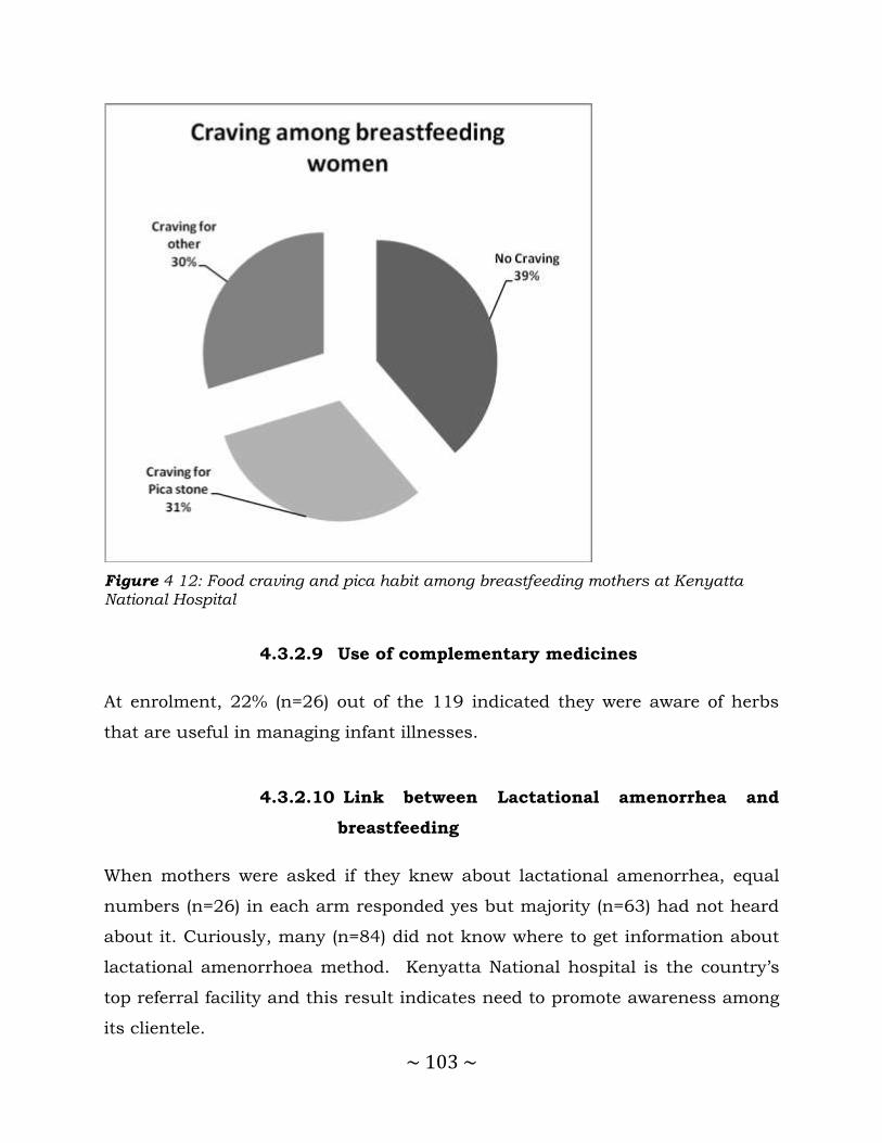
~ 103 ~

Figure 4 12: Food craving and pica habit among breastfeeding mothers at Kenyatta National Hospital

4.3.2.9 Use of complementary medicines

At enrolment, 22% (n=26) out of the 119 indicated they were aware of herbs

that are useful in managing infant illnesses.

4.3.2.10 Link between Lactational amenorrhea and

breastfeeding

When mothers were asked if they knew about lactational amenorrhea, equal

numbers (n=26) in each arm responded yes but majority (n=63) had not heard

about it. Curiously, many (n=84) did not know where to get information about

lactational amenorrhoea method. Kenyatta National hospital is the country’s

top referral facility and this result indicates need to promote awareness among

its clientele.

~ 104 ~

More mothers 68% (n=81) made one to two antenatal visits. This is an

important factor in determining the quality of monitoring during pregnancy to

help identify those likely to develop complications during delivery.

4.3.2.11 Use of Iron supplements

Iron was taken by 58% (n=69) of the mothers, while 49% (n=58) took folic acid

prior to joining the study. This is further analyzed in chapter 5.

The information gathered on use of herbs was found to have a very strong

association with the maternal hematology. This is also analyzed in chapter 5 of

this report.

4.4 Discussion and conclusion

This baseline of the study participants in the Chinsaga clinical trial sought to

describe the demographics and nutritional behavior of mothers attending the

postnatal clinic at Kenyatta National Hospital that may have a bearing on the

hematological and lactational outcomes of this study.

Not many peer reviewed publications are available on the fruit and vegetable

eating habits of Kenyans in Nairobi but one report by Ayieko et al (6) attempts

to provide some information and is used as a comparator to data collected in

this study.

Mothers in the population mostly consumed Kale and cabbage as the vegetable

component of their diet. Tomatoes and onions are universal while kale, cabbage

carrots and bananas follow in decreasing order (6). Sukuma wiki (Kale) is the

most consumed leafy vegetables justifying its use as the control in this study.

Among fruits, bananas and oranges are the most consumed followed by

mangoes, papaws and avocadoes in decreasing order of frequency. About a

~ 105 ~

third of household food expenditure is on dairy products, meat and eggs;

another third on fresh produce that constitute staples and a quarter on fresh

fruits and vegetables.

Ayieko et al (6) also showed a range from 15% for the lowest quintile to 6% for

the highest quintile in the expenditure of households on basic foods with most

going to dairy products and within this milk was the prime item. Lower income

groups were found to spend more on maize. The expenditure on maize

diminishes with rise in income as wheat, rice, beef, mutton and poultry

products become more popular among the high income groups.

Studies have been conducted elsewhere to evaluate nutritional practices. One

such study looked into consumption of fruits and vegetables among school

children of Asian countries and found Thai school children had the highest rate

of fruit and vegetable consumption. It is thought that availability and income

may be the key determinants of vegetable consumption and this collated with

findings by others in the same country (16) . It is important to note that, the

Thai government instituted a national policy promoting consumption of fruits

and vegetables resulting in steady rise in the rate of consumption of fruits and

vegetables since 1986 and may be worth emulating in Kenya.

The highest consumed fruits among mothers in this study were oranges 87%

(n=104) and avocado 71% (n=84) Fruit consumption is determined mainly by

family income, preferences and market prices(6). Preferences were affected by

composition of the household, its member’s knowledge education, habits and

cultural norms, personal experience and biological drivers of hunger. Fruits

and vegetables are considered a pricier source of energy especially among poor

households. At these levels, larger amounts of starchy foods and grains were

consumed.

~ 106 ~

Fruits and vegetables are a rich source of provitamin A (carotenoids). The

relationship between carotenoids taken in from plant foods and the status of

vitamin A was tested in breastfeeding women in rural Vietnam. Changes in

blood and breast-milk retinol concentrations suggested lower bioavailability of

carotenoids from vegetables and fruit than previously assumed (17).

Considering the survey was conducted in Nairobi, the food eating patterns are

highly influenced by multiple cultures and key among them are communities

from central Kenya. Thus the foods seen in the survey are very similar to those

collected in the present study conducted among women attended at Kenyatta

National Hospital. One example in the consistency of Irish potatoes in the diet

seen across all income groups. The proportion of budget spent on vegetables is

expected to decline as one climbs up the income groups. This is probably

because the absolute expenditure may rise but less so in proportion to the total

income (18).

Diet rich in fruits is generally pricy in Nairobi. Ayeiko et al (6) also observed

food spendings on dairy products, vegetables, beef, wheat products, maize

products, and fruits similar to findings in this study at Kenyatta National

Hospital. Most paticipants responded positively for these items in the food

questionnaire. Rise in incomes, were also noted to lead to more meats, animal

products and fruits incluion diet.

According to Ayieko et al (6), there was association between educational level of

the head of household and expenditure on fresh produce. Female headed

households tended to have more fruit and fresh vegetables despite income

levels. This finding may be an indicator of economic independence among

women with higher incomes, and probably also reflects different decision

making processes regarding consumption in households where a woman is the

primary decision maker.

~ 107 ~

There was no systematic pattern between age of the head of a household and

income but Ayieko et al (6) noted decreased expenditure on fresh fruits and

vegetables in homes with more children which is expected. However in this

study, the measure of RBC discussed in chapter 5 indicated a higher RBC

count with increasing age of husband.

In a study carried out across several African countries, the percentage of

households consuming fruits was found to vary from about 20% in Ethiopia,

Mozambique to about 50% in Rwanda, Kenya and Malawi, and about 75% for

Tanzania and Guinea. When results for vegetables are included, the

percentages are well over 90%. It is notable that among the countries surveyed,

including Ethiopia, Burundi, Malawi, Mozambique, Tanzania, Rwanda,

Uganda, Ghana and Guinea, Kenya had the highest consumption per capita

per year of 25.8 Kg/person/year for fruits and 88.3 Kg/person/year for

vegetables. It was also one of the countries that exceeded the minimum

recommended level of 146Kg/person/ year. It was also observed that many

families spend on fruits and vegetables ranging from 43% in Guinea to 73% in

Burundi. Diets in urban areas are generally more diverse than those in rural

areas (19). This is associated with greater availability of supply converging to

the urban markets. A rich variety of fruits were listed for comsumption among

mothers involved in this study.

Differences between rural and urban consumption was observed to be largest

in Kenya and Burundi. Income differentials were also observed to affect

percentages within countries. Fruit and vegetable consumption tended to

increase with income (19). Family size was observed to have a negative

association with proportion of income spent on fruits and fresh vegetables.

Surprisingly, in this study presence of a household member with higher than

secondary education, was associated with lower allocation to fruits and

vegetables. Valuable information may be derived from a study to assess the

effect of such a person on the decision making processes and resource

~ 108 ~

allocation resulting in this disparity. Part of this may be the expectation that

such a person may be the leader in the home and the major breadwinner.

From the recent past, consumers have become increasingly aware of the

nutritional and medicinal value of African indigenous vegetables in bridging the

gap of micronutrients among African households (20). African indigenous

vegetables are known for their importance in providing nutritious food, both in

rural and urban areas. The vegetables play a crucial role in income generation

and subsistence. Some of them have been attributed with having medicinal-

value properties and are grown for home consumption (21). They are

considered traditional crops because some of the vegetables were planted;

others were readily available and harvested in their habitat appearing as

volunteer crops or weeds. Others had been consumed for countless generations

signifying their value and importance in local cultures (22).

Increasing popularity of traditional leafy vegetables has caused a rise in

demand especially in major urban centers. The supply of these vegetables has

however not matched this growing demand (23). Most farmers are semi

commercially oriented poor farmers, are not organized, and lack inputs and

skills to enable them to satisfy the dynamic market requirements. They are not

able to access high value markets such as supermarkets and are often

exploited by middlemen responding to the changing consumption patterns and

market opportunities occasioned by the growing demand for these vegetables in

the urban centers (4,24). Consumption of traditional vegetables and grains was

established to be lower than kale and cabbage among the praticipants

In conclusion, foods and diet items vary with culture. Across Kenya and in

Africa, maize, sweet potato, sorghum, millet and cassava are among the most

popular foods. Vegetables used traditionally are also rich sources of vitamins

such as pro-vitamin A from Chinsaga. Promoting the use of such vegetables is

~ 109 ~

an important part of a multipronged approach to address the gap in supply of

such nutrients.

Recommendations from this study include public awareness creation, active

government policy to facilitate and promote consumption of fruits and

vegetables with a greater emphasis on production and distribution of

traditional varieties. The Ministry of Health needs to carry out public re-

education on the importance of breastfeeding and its contribution as a natural

form of family planning.

4.5 References

1. (Nairobi) KNB of S. Kenya Demographic and Health Survey 2008-09. Kenya National Bureau of Statistics; 2010.

2. Rush D. Nutrition and maternal mortality in the developing world. Am J Clin Nutr. 2000;72(1):212s – 240s.

3. Chersich MF, Kley N, Luchters SMF, Njeru C, Yard E, Othigo MJ, et al. Maternal morbidity in the first year after childbirth in Mombasa Kenya; a needs assessment. BMC Pregnancy Childbirth. 2009;9:51.

4. Abukutsa-Onyango MO. Market survey on African indigenous vegetables in Western Kenya. Proceedings of the second Horticulture seminar on Sustainable Horticultural production in the tropics JKUAT [Internet].

2002 [cited 2013 Sep 4]. p. 39–46. Available from: http://www.gem.uni-hannover.de/fileadmin/institut/gemuesebau/pdf/SVepit/Proceedings200

2.pdf#page=47

5. FAO/WHO Workshop on Fruit and Vegetables for Health. Fruit and vegetables for health report of a joint FAO/WHO workshop, 2004, Kobe,

Japan. Geneva: WHO; 2005.

6. Ayieko MW, Tschirley DL, Mathenge MW. Egerton University. [cited 2013

Oct 3]; Available from: http://ageconsearch.umn.edu/bitstream/55164/2/wp19.pdf

7. McNeilly AS, Tay CC, Glasier A. Physiological mechanisms underlying

lactational amenorrhea. Ann N Y Acad Sci. 1994 Feb 18;709:145–55.

~ 110 ~

8. McNeilly AS. Lactational amenorrhea. Endocrinol Metab Clin North Am. 1993;22(1):59.

9. Perez A, Labbok MH, Queenan JT. Clinical study of the lactational amenorrhoea method for family planning. The Lancet.

1992;339(8799):968–70.

10. Labbok MH, Perez A, Valdes V, Sevilla F, Wade K, Laukaran VH, et al. The lactational amenorrhea method (LAM): a postpartum introductory family

planning method with policy and program implications. Adv Contracept. 1994;10(2):93–109.

11. Kazi A, Kennedy KI, Visness CM, Khan T. Effectiveness of the lactational

amenorrhea method in Pakistan. Fertil Steril. 1995;64(4):717.

12. Labbok MH, Hight-Laukaran V, Peterson AE, Fletcher V, von Hertzen H,

Van Look PF. Multicenter study of the Lactational Amenorrhea Method (LAM): I. Efficacy, duration, and implications for clinical application. Contraception. 1997;55(6):327–36.

13. Peng Y-K, Hight-Laukaran V, Peterson AE, Pérez-Escamilla R. Maternal Nutritional Status Is Inversely Associated with Lactational Amenorrhea in

Sub-Saharan Africa: Results from Demographic and Health Surveys II and III. J Nutr. 1998 Oct 1;128(10):1672–80.

14. Diaz S, Cardenas H, Brandeis A, Miranda P, Schiappacasse V, Salvatierra

AM, et al. Early difference in the endocrine profile of long and short lactational amenorrhea. J Clin Endocrinol Metab. 1991;72(1):196–201.

15. Pinheiro J, Seabra D. [Changes of food habits during pregnancy and

breast-feeding]. Acta Médica Port. 2008 Apr;21(2):149–60.

16. Bloem MW, Wedel M, Egger RJ, Speek AJ, Schrijver J, Saowakontha S, et

al. Iron metabolism and vitamin A deficiency in children in northeast Thailand. Am J Clin Nutr. 1989 Aug 1;50(2):332–8.

17. Khan NC, West CE, Pee S de, Bosch D, Phuong HD, Hulshof PJ, et al. The

contribution of plant foods to the vitamin A supply of lactating women in Vietnam: a randomized controlled trial. Am J Clin Nutr. 2007 Apr 1;85(4):1112–20.

18. Muyanga M, Jayne TS, Argwings-Kodhek G, Ariga J. Staple food consumption patterns in urban Kenya: Trends and policy implications

[Internet]. Tegemeo Institute of Agricultural Policy and Development; 2006 [cited 2014 Nov 20]. Available from: http://fsg.afre.msu.edu/kenya/WPS19.pdf

~ 111 ~

19. Ruel MT, Minot N, Smith L. Patterns and determinants of fruit and vegetable consumption in Sub-saharan Arica: a multicountry comparison.

International Food Policy Research Institute; 2004.

20. Fondo J, Morimoto Y, Maundu P. Documenting The Diversity Of

Traditional Leafy Vegetables And Fruit Trees Used By Giryama Communities Of Coastal Kenya: A Community-Led Ethnobotanical Research And Development Initiative. Symposium Proceedings, The 10th

International Congress of Ethnobiology Chiang Rai, Thailand. 2006. p. 5–9.

21. Chweya JA, Eyzaguirre PB. The biodiversity of traditional leafy vegetables.

[Internet]. IPGRI; 1999 [cited 2013 Aug 25]. Available from: http://www.cabdirect.org/abstracts/20036794474.html

22. Ayodele AE. The Medicinally Important Leafy Vegetables of Southwestern Nigeria. Ethnobot Leafl. 2005;2005(1):16.

23. Tschirley DL, Ayieko MW, Mathenge MW, Weber M. Tegemeo Institute -

Where do Consumers in Nairobi Purchase their Food and why does this matter? The Need for Investiment to Improve Kenya’s Traditional Food

Marketing System [Internet]. 2004 [cited 2013 Oct 3]. Available from: http://www.tegemeo.org/index.php/research-resources/publications/item/99

24. Dinham B. Growing vegetables in developing countries for local urban populations and export markets: problems confronting small-scale producers. Pest Manag Sci. 2003 May;59(5):575–82.

~ 112 ~

CHAPTER FIVE

5.0 Effects of Chinsaga (Gynandropsis gynandra) on

hematological indices

~ 113 ~

5.1 Introduction and literature review

5.1.1 Role of Iron in Red Blood Cell Physiology

Iron is essential for oxygen transport and cell growth and survival. The typical

adult human body contains an average of 3.5 g of iron (approximately 4 g for

males and 3 g for females). Most of the iron within the body is used in

haemoglobin (2.1 g) synthesis. A small amount is devoted to cellular protein

synthesis (myoglobin, cytochromes) or circulates through plasma bound to

transferrin (1). Iron homeostasis is closely regulated via intestinal absorption

and by recycling of iron already present in the body. This element has the

particularity that once absorbed; there is no physiologic mechanism for its

excretion from the body. Males loose less iron (1 mg/day) compared to an

average of two mg/day by women during their menses.

To maintain adequate supplies of iron for heme synthesis, 20 mg of iron is

recycled daily, going from senescent red cells that are removed from the

circulation to new cells in the bone marrow (2). Iron from older cells is loaded

onto transferrin by macrophages for delivery to the bone marrow. The diet

provides 10–20 mg per day of iron requirement, as heme (mainly in red meat)

and non-heme (white meat, vegetables, and cereals). Healthy adults absorb

approximately 10 to 15% of this iron in their diet, but absorption is influenced

by the body’s iron stores, the type of iron in the diet (heme and non-heme), and

other dietary factors that may increase or reduce the absorption of iron. Heme

iron is absorbed very efficiently by the body whereas only 1 to 7% of non-heme

iron is absorbed (3).

~ 114 ~

5.1.2 Anemia in Pregnant and Lactating women

Prevalence and complications of Iron deficiency anaemia (IDA) are the most

common type of mortalities associated with anaemia arising when there is

insufficient iron to support normal red cell production. According to the World

Health Organisation (4), iron deficiency is the most common form of

malnutrition in the world, affecting around 2 billion people (25% global

population) worldwide.

It is of particular concern among women and children. Pregnancy and

increased bleeding during menstruation confer women a higher risk of

developing IDA leading to high morbidity and mortalities. Mothers with anemia

have an increased risk of complications during pregnancy and delivery.

Maternal anemia has been considered as a risk factor for an undesirable

pregnancy outcome (5).

5.1.3 Diagnosis of Anaemia in Pregnant and Lactating mothers

Many women remain undiagnosed due to the reliance on conventional

parameters, such as the post-delivery serum ferritin. As an inflammatory

protein, ferritin is artificially raised after delivery (6). This enhances the

potential for false results. It is therefore advisable to test for post-delivery

serum ferritin at least four weeks after delivery.

Judgment about clinical iron status in pregnancy is often clouded by factors

such as hemo-dilution and the observation that even apparently high Hb,

mothers may be suffering iron deficiency.

Hematocrit is found to provide a better estimate than hemoglobin to get a

measure of the red blood cell volume to total blood volume. Besides hematocrit,

other parameters that affect rheology of blood include blood cells

~ 115 ~

concentration, dimensions of blood vessels and flow and plasma concentration.

Changes in these parameters may therefore serve as indicators of possible

danger during pregnancy (7).

Considering the high prevalence of anemia during pregnancy worldwide, one

study was carried out to compare detection of iron deficiency during pregnancy

with hemoglobin (Hb) and serum measurements considering the effects of

hemodilution or accelerated erythropoiesis. It was to determine whether cell

indices will give a more reliable measure of iron deficiency in pregnant women

at term (8).

According to the Krafft study (9), results provided by the cell indices alone of

Percentage of Hypochromic Red Blood Cells (%HYPOm or CHr) were in good

agreement with the results based on the combination of three commonly used

tests (Hb, MCV, ferritin). These findings of their study suggested use of cell

indices such as CHr and %HYPOm provided by the automated hematological

analyzer as the most practical way to diagnose iron deficiency in pregnant

women at term but would need additional work to determine their utility in

monitoring trends helpful in diagnosis of iron deficiency during the course of

pregnancy.

5.1.4 Debate over benefits of iron and folic acid

supplementation

Suggestions have been made to have iron supplementation for pregnant

women, young children and adolescents universal in countries where the

prevalence of anaemia in the population is over 40% because of the presumed

challenge in providing sufficient amounts through the regular diet.

The benefits of iron supplementation in pregnancy and lactation remain a

debatable issue in perinatal medicine in reducing the prevalence of iron

~ 116 ~

deficiency anaemia. The results of supplementation programmes have often

proved disappointing, especially in developing countries, (10,11), despite the

evidence of benefit in terms of red cell and iron parameters in pregnancy and

lactation (12). What is lacking, however, is proof of the benefit of postpartum

iron supplementation in the women with non-anaemic iron deficiency at term

that form a substantial proportion of the obstetric population, even in

industrialised countries.

The 1999 Cochrane Database found no case for routine iron supplementation

in developed countries with a balanced dietary and micronutrient intake (13).

In countries with poorer antenatal care, compliance to iron supplementation is

low. In Brazil, Trugo (14) found that 80–160 mg/day of iron failed to lower the

incidence of third trimester iron deficiency in non-anaemic healthy women

compared with controls, concluding that supplemental iron served to supply

the red cells, fetus and placental tissue rather than replenish the iron stores.

5.1.5 Iron formulations and salts

Various iron formulations are commercially available and their efficacy and

tolerability have been tested in several studies. The most common way to

correct for iron deficiency anaemia, is to replenish the iron usually by oral

administration of ferrous formulations. Intravenous administration has the risk

of causing the undesirable state of iron overload. Unfortunately, most

formulation of either ferrous (divalent) or ferric iron have erratic bioavailability

especially the ferric types and this reduces compliance among most patients.

The most common side effects of oral iron therapy are gastrointestinal

disturbances including constipation, diarrhea nausea, heartburn and gastric

pain.

Divalent iron is more commonly prescribed as the ferrous salt, gluconate or at

times, fumarate. They are generally better absorbed than the trivalent ferric

~ 117 ~

preparations due to poor solubility of ferric ions in the alkaline conditions of

the small intestines. In addition ferric iron must be transformed into ferrous

iron to be absorbed across the gut mucosa. One major drawback to use of iron

formulations is the nausea and intestinal discomfort associated with their use.

Most manufacturers have attempted to improve the formulations to reduce

these effects.

Studies have been made (15) evaluating quick versus slow release iron and

found minimal difference in effect after 21 days. They observed that

haemoglobin levels increased to near baseline values after two months of

treatment in both treatment groups.

Iron coupled with sugar complexes has been compared to ferrous formulations

in several studies and found to have very low efficacy contrary to expectations.

Trivalent iron is believed to be more stable and easier to carry across the

intestinal mucosa. In 2003, Mehta’s (16) report of 27 patients who failed to

respond to iron coupled with sugar complexes given for 4 to 52 weeks but later

responded to ferrous fumarate for 4 to 13 weeks. Ruiz-Argüelles et al (17)

showed a 31% failure rate with better response when switched to ferrous

fumarate.

A study (15) using 59Fe III hydroxide-polymaltose showed a near 40 fold

difference in absorbtion in the fasted state. The difference reduced when the

iron was taken with food. In another study (18), haemoglobin levels failed to

increase in 9 patients receiving 100 to 300 mg of ferric polymaltose complex

over a four week period. At week 9 the difference between both groups was not

statistically significant.

~ 118 ~

5.1.6 Association between maternal iron levels and farming

practices.

One study conducted among the Pokot in Kenya (19), Ettyang et al found

women from the farming community in West Pokot, Kenya, had lower

hemoglobin and serum ferritin concentrations in the third trimester of

pregnancy and four months postpaterm than women in the pastoral

community. However, no differences were observed in serum retinol levels.

Notabley, the farming community had a significantly higher proportion of

newborns weighed less than 2.5 kg compared to the pastoral community.

5.1.7 Hematological biomarkers of iron metabolism

The hematological indices that are related to erythrocytes are: RBC; hemotocrit;

hemoglobulin levels, mean corpuscular volume (MCV), mean corpuscular

hemoglobin (MCH), Red blood cell distribution (RDW); and Mean Corpuscular

Hemogloblin Concentration (MCHC). MCHC is diminished in microcytic

anemia. It is a more reliable indicator of anaemia because levels remain low

even though the hemboglobulin and MCH levels are high. The reference values

for MCHC range from 32 to 36 g/dL or 4.9 – 5.5 mmol/L. It is calculated by

dividing MCH with the RBC.

Mean corpuscular volume is obtained by dividing hemotocrit by the RBC. RDW

is an additional measure of red blood cell volume. The usual size of the human

red blood cell is 0 to 8 micrometers. The reference range of RDW values in

humans is 11 – 15%. Both MCV and RDW are used to determine the cause of

anemia. In macrocytic anemia caused by Vitamin B12 or folic acid deficiency,

RDW values are high. MCV is obtained by dividing the hemocrit with the RBC.

The reference range for MCV is 80 – 100 fL.

RDW is calculated using the formula below:

~ 119 ~

RDW = (Standard deviation of MCV / Mean MCV) X 100

Population values of hemoglobin range from 12 to 16 grams per deciliter for

women of childbearing age with the minimum about 11 grams per deciliter in

the first and third trimester of the pregnancy and 10.5 grams per deciliter in

the second trimester of pregnancy (21).

Anemia is the leading cause of low values of hemoglobin while erythrocytosis

triggered by chronic obstructive pulmonary disease myeloproliferative disorders

and other hypoxic lung conditions may lead to abnormally raised Figures

during tests. It may be prudent to include socioeconomic and anthropological

factors in the forecast when making such interpretations especially in a varied

society as that found in Kenya.

Plasma volume is an important factor in determining hemoglobin levels and

hematocrit which requires fresh whole blood for determination.

5.1.8 Problem statement

In many African communities there are beliefs that some plants promote

lactation and aid recovery from post-delivery anemia. However there is lack of

clinical evidence about these claims. This may therefore lead to unsupported

use of these plants. If indeed such plants are beneficial, this knowledge should

be made widely available as a strategy to combat postnatal complications such

as anemia. Chinsaga is widely used by the Kisii for its claimed benefits in

improving lactational and pregnancy outcomes. This study therefore sought to

determine if use of this vegetable is clinically beneficial.

~ 120 ~

5.1.9 The Null hypothesis

There is no difference on the hematological profile of breastfeeding mothers

taking Chinsaga (Gynandropsis gyanandra) compared to those on Kale over 28

days.

5.1.10 Research Objectives

The main objective was to compare the effects of Chinsaga (Gynandropsis

gynandra) to Kale (Brassica carinata) on haematological profile of breastfeeding

women.


1. To compare the effects of Chinsaga (Gynandropsis gynandra) and Kale on

the selected hematological parameters such as hemotocrit, mean

corpuscular hemoglobin and hemoglobin levels.

2. To identify which hematological parameter is most affected by

supplementing the diet of mothers with Chinsaga

3. To determine if there is biological interaction between iron

supplementation and use of Kale or Chinsaga.

5.1.12 Study Justification

The findings of this study are expected to guide policy makers on optimal local

nutritional interventions that may reduce the incidence of post-natal anaemia,

~ 121 ~

5.2 Materials and methods

5.2.1 Ethical considerations

The study was conducted with approval from Kenyatta National Hospital –


ERC/01/3757) and the Kenyatta National Hospital clinical services department

as mentioned in Chapter 4.

Mothers were informed about the study and again asked if they still wish to

join the study. Participants were required to give informed and documented

consent. They were allowed to make this decision at another visit if unable to

do so on the first day. During all aspects of sample handling, only numbers

were used to track the records of the participants.

5.2.2 Study design

This study was a randomized triple blinded placebo controlled study involving

lactating mothers attending Kenyatta National Hospital Maternal Newborn

Child Health (MNCH) clinic. There were two study arms. One arm was treated

with placebo which was cooked dried kale and the second arm was treated with

Chinsaga.

5.2.3 Study site and duration

The study was conducted in Kenyatta National Hospital which serves mainly

women from Nairobi and its environs. Participants were recruited from the

Maternal Newborn Child Health (MNCH) clinic. This study was conducted over

a period of four months, July to November 2008.

~ 122 ~

5.2.4 Inclusion and Exclusion criteria

The study targeted healthy women, free from chronic disease with exception of

asymptomatic HIV positive mothers. They should not have been on Chinsaga at

least four weeks prior to enrollment, willing to give consent, available for six

months within the environs of Nairobi city and should not be smoking

cigarettes.

Mothers were excluded from the study if they were not breastfeeding, smoked

cigarettes, and suffered chronic illness such as Rheumatoid arthritis, Crohn's

disease, colitis ulcerosa, diabetes, asthma and hypertension. They were also

excluded if they were on prescription medication or non-steroidal anti-

inflammatory drugs on a regular basis, using vitamins or mineral supplements

for the last one month, corticosteroids or on immunostimulators for the last 4

weeks or their hemoglobin concentration was below 8g/dL. Positive HIV status

was not an exclusion criterion.

5.2.5 Sample size considerations

One of the major benefits expected in the Chinsaga treatment group is a rapid

improvement in hemoglobin levels. Sample size was calculated using the proof

of concept model. A major benefits expected in the Chinsaga treatment group

was a more rapid improvement in hemoglobin levels. With normal hemoglobin

concentration range from 9.5-15.8 g/dL (22), difference of 1.5 g/dL between

the Kale (Group 1) and Chinsaga (Group 2) and variance of 1.5 g/dL, power of

80%, confidence level of 95%, and correcting for a 25% dropout rate, a sample

size of 22 was calculated as the minimum to differentiate between the

experimental and control groups, we would require 22 women participants in

each of the two groups.

~ 123 ~

5.2.6 Participant recruitment

Mothers attending the Maternal Newborn Child Health (MNCH) clinics were

informed about the study and asked if they are interested in taking part in the

study. Those that accepted to join the study were screened for eligibility. Those

that qualified for recruitment were adequately informed of the study as

outlined in Chapter 4. About 115 healthy subjects were enrolled after screening

for eligibility with 37 completing the follow up for 28 days thereafter.

5.2.7 Randomization and treatment allocation

The randomization scheme was generated by a volunteer working as an IT staff

within a clinical trial independent from the investigator and the list printed and

copies made for use during the work by using the Web site Randomization.com

(23) (24) ⟨http://www.randomization.com⟩ by Gerard E. Dallal and last

updated on 07/16/2008 05:07:20.

The volunteer mothers were divided into two treatment groups: Chinsaga and a

control group on Kale (Brassica oleracea). A block randomization (5 subjects in

each block) was used to assign women into either the kale - placebo (group

one) or the Chinsaga – test (group two). Study volunteers were allocated to

treatment groups according to the list and after consenting to participating in

the study. Each volunteer was sequentially assigned a number and the

corresponding treatment given using the randomization list.

5.2.8 Blinding and Allocation concealment

In order to achieve maximal level of blinding, several measures were taken to

achieve triple blinding. During the preparation, materials for the study were

packed in identical sachets. The sachets were all marked with the single digit 1

which whose position was varied slightly depending on the two treatments. The

~ 124 ~

distinction between both packets was adequately masked unless one was given

prior information. The study staff would only know the treatment group but

were blinded as to which of these was intervention or control.

The treatment material was packed in sachets that were similarly marked and

practically indistinguishable unless prior information was given to those

participating in administering or taking the materials. The mark to distinguish

the two materials was kept sealed from the investigators. This was important to

prevent confusion during packing the study sets and allow cross-checking

during the dispensing.

Information about the meaning of the codes, treatment or control arms was

kept from the data analyst until data analysis was complete. Directions to help

disclosure were sealed except to workers at the firm packing the treatment

sets. A closed envelope was provided for use during un-blinding to the

supervisor of the study for safekeeping until the end of the data analysis of the

study. At this point, disclosure was sought to help determine effect of the

intervention. Directions for disclosure were sealed except to workers of the

packing firm for the treatment sets.

5.2.9 Data collection

The study staff that facilitated the conduct of the research were recruited and

trained appropriately. They were formally introduced to the clinic and other

hospital staff, and were involved in a study conducting preliminary pilot review

of work and fine tuning of documentation and study procedures.

~ 125 ~

5.2.10 Administration of Study products

Study participants were given sachets of prepared Chinsaga daily for the test

group and Kale for the control group for 4 weeks. Each member of the

Intervention group was given a 9gram sachets made from dried Chinsaga to be

taken taken for 28 days from the day of recruitment. Each member of the

control group was given a 9 gram placebo sachets made from dried kale taken

for 28 days.

Participants were given directions on how to take the study products with their

main meal and to report if they encountered any challenges or problems during

the entire intervention period. The participants were required to make at least

three scheduled study visits at screening and enrolment at enrollment (day 0),

first follow up at day 14 and the final follow up at day 28.

5.2.11 Collection and analysis of biological specimens

Blood samples, 5ml, were collected in EDTA tubes (VacutainerTM, Becton

Dickinson Vacutainer Systems, Plymouth, UK) for a complete blood cell count,

including analysis of red blood cell and reticulocyte parameters obtained with

an Act 5 B Hematology Becton Dickinson System. The serum samples,

collected in serum tubes (VacutainerTM, Becton Dickinson Vacutainer Systems),

were centrifuged and the serum was separated and stored frozen at −70°C.

Transferrin, ferritin and lactoferrin from breast milk samples were analysed as

detailed in chapter 6 of this report.

5.2.12 Data analysis

Data analysis was conducted on all variables to generate summaries of

findings. Kruskal wallis test was used to test for differences across arms

because most of the outcome variables were not normally distributed. Sub-

~ 126 ~

group analysis was done in which the baseline characteristics of participants

who came for Day 14 was compared. This was done to rule out the fact that

there could have been systemic differences at baseline values in individuals

who completed the study.

In order to select which outcome variable was affected by treatment, the

outcome variables were subjected to generalized linear regression analysis with

treatment group as the dependent variable and time of visit as the independent

variable. Variables where the p value of the treatment variable was less than

0.05 were subjected to modeling using a forward step wise approach.

Generalised linear modeling was done to control for confounding. The variables

were first transformed so that they could be normally distributed.

An additional component of data analysis sought to determine if the effect of

treatment assignment were confounded and if there was biological interaction

with known hematinic agents and other socio-demographic and nutritional

factors. The presence of confounding was evaluated by generating a regression

model that had treatment assignment and a putative confounder as the only

covariate variables. A variable was considered to be a confounder if the

percentage change in the crude beta coefficient of the treatment variable was

greater (10%).

In order to determine that there was statistical interaction between treatment

and other covariates, an interaction term was generated from the product of

treatment and a covariate. If the interaction term was statistically significant,

statistical interaction was deemed to be present.

~ 127 ~

5.3 Results

5.3.1 Randomization of study participants

Study participants were randomized as illustrated in the consort diagram

Treatment 1 (Kale), Treatment 2 (Chinsaga) (Figure 5.1).

Figure 5 1: Consort diagram of randomisation and follow up of study volunteers into kale (Control) and Chinsaga (Test) at KNH on days 0, 14 and 28.

The baseline characteristics across the study arms are summarized in chapter

4 of this thesis

~ 128 ~

5.3.2 Effects of Chinsaga on selected Red Bloodcell Count

related parameters

The focus of analysis was mainly on the effects of Chinsaga treatment on

hematological indices related to erythrocytes. The variables that were used as

markers of iron metabolism were: hematocrit (HC), hemoglobin levels (Hb),

MCHC, MCV, RDW and RBC counts. Table 5.1 summarizes the differences

across arms during the 3 study visits.

Table 5 1: Differences in selected hematological parameters in patients treated with Chinsaga and Kale over 28 days

Blood parameter Duration Kale Chinsaga P

HEMATOCRIT Baseline 37.3 (IQR 33.4–40.3) 37.4 (IQR 34.1–39.5) 0.75

Day 14 40.25 (IQR 33.0–42.15) 39.7 (IQR 35.3 – 41.1) 0.91

Day 28 37.8 (IQR 31.8 – 40) 39.9 (IQR 36.8 – 40.3) 0.31

HEMOGLOBIN Baseline 12.7 (IQR 11.4 – 13.7) 12.5 (IQR 11.5 – 13.6) 0.33

Day 14 13.6 (IQR 10.75–14.55) 13.4 (IQR 11.0 – 13.8) 0.60

Day 28 12.6 (IQR 10.6 – 13.6) 13.3 (IQR 12.4 – 13.9) 0.42

RDW Baseline 13.5 (IQR 12.5 – 15.1 ) 13.4 (IQR 12.6 – 14.8 ) 0.86

Day 14 13.6 (IQR13.05 – 14.6) 14.8 (IQR 13.05 – 16.9) 0.08

Day 28 13.7 (IQR 11.7 – 14.8) 14.6 (IQR 13.5 – 16.3) 0.05

MCV Baseline 85 (IQR 78 - 88) 82 (IQR 78 – 88) 0.11

Day 14 84 (IQR 78.5 – 88) 80 (IQR 76 – 83) 0.07

Day 28 85 (IQR 77 – 89) 79 (IQR 77 – 83) 0.08

MCHC Baseline 34 (IQR 33.5 – 34.5) 33.7 (IQR 33.2 – 34.3) 0.05

Day 14 34.05 (IQR 33.15–34.6) 33.7 (IQR 33.2 – 34.2) 0.11

Day 28 34 (IQR 33.4 – 34.4) 33.4 (IQR 33.2 – 34.4) 0.22

MCH Baseline 28.2 (IQR 26.4 – 30.2) 27.8 (IQR 25.8 – 29.1) 0.09

Day 14 28.65 (IQR 26.4 – 30.4) 27 (IQR 25 – 28.4) 0.03

Day 28 29 (IQR 26.6 – 30.3) 27.3 (IQR 25.5 – 28.6) 0.05

RBC Count Baseline 4.38 (IQR 4.18 – 4.98) 4.56 (IQR 3.79 – 5.26) 0.25

Day 14 4.6 (IQR 4.69 – 5.76) 4.91 (IQR 4.69 – 5.08) 0.03

Day 28 4.5 (IQR 4.37 – 4.81) 4.91 (IQR 4.8 – 5.08) 0.03

The only parameters for which there was no statistically significant difference

across study arms were: haemotocrit; hemoglobin; and MCHC. The parameters

for which there was a statistically significant difference across study arms by

Day 28 were: RBC count; MCH; and RDW. In the case of RBC counts and

MCH, the median values of patients treated with Chinsaga were statistically

~ 129 ~

higher than the values of patients treated with Kale by day 14 and later on day

28 of the study.

The Kale-treated arm had higher MCV values and lower RDW values by Day

28. In addition, the Kale treated arm had higher median MCHC and MCH

values compared to the Chinsaga treated arm by Day 28. High MCV and RDW

values are indicative of macrocytic anemia caused by deficiency of Vitamin B12

and/or folic acid. Hematocrit of the Chinsaga treated arm was also higher in

the third visit

5.3.3 Longitudinal changes in Hematological parameters

5.3.3.1 Changes in Hemotocrit and Hemoglobulin levels

As previously stated, there was no statistically significant difference in the

hemotocrit and hemoglobulin levels by Day 28 compared to the control. The

median levels and IQR for these two parameters at each of the visits are

illustrated in Figure 5.2 As can be seen, both the values of both these

parameters increased during the course of the study compared to the baseline

value.

Figure 5.2a Group one (Kale), Group two (Chinsaga).

~ 130 ~

Figure 5.2 b Group one (Kale), Group two (Chinsaga).

Figure 5 2: Median changes in Hemotocrit and Hemoglobin levels Kale (Group one), Chinsaga (Group two).

5.3.3.2 Longitundinal changes in Red Bloodcell Count

Figure 5 3: Longitundinal changes in the Red Blood Cell count (Group one - Kale, Group two - Chinsaga).

In the Chinsaga treated arm, there was a noticeable increase in the RBC count

from baseline. An increase was also noted for the Kale treated arm but the rate

of increase seemed slower, Figure 5.3.

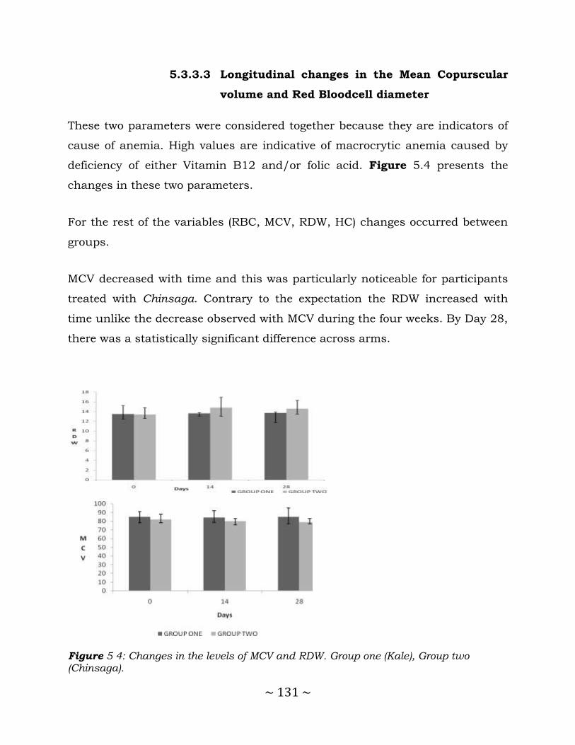
~ 131 ~

5.3.3.3 Longitudinal changes in the Mean Copurscular

volume and Red Bloodcell diameter

These two parameters were considered together because they are indicators of

cause of anemia. High values are indicative of macrocrytic anemia caused by

deficiency of either Vitamin B12 and/or folic acid. Figure 5.4 presents the

changes in these two parameters.

For the rest of the variables (RBC, MCV, RDW, HC) changes occurred between

groups.

MCV decreased with time and this was particularly noticeable for participants

treated with Chinsaga. Contrary to the expectation the RDW increased with

time unlike the decrease observed with MCV during the four weeks. By Day 28,

there was a statistically significant difference across arms.

Figure 5 4: Changes in the levels of MCV and RDW. Group one (Kale), Group two (Chinsaga).

~ 132 ~

5.3.3.4 Longitudinal changes in Mean Corpuscular

Hemoglobin and Mean Copurscular Hemoglobin

Concentration

MCHC and MCH declined with time in the Chinsaga treated arm compared to

Kale treated arm where it remained fairly constant, Figure 5.5. This decrease

could be attributed to the rapid increase in the RBC count in patients treated

with Chinsaga without a corresponding increase in Hb. MCHC is calculated by

dividing MCH with the RBC and is the most reliable measure of anaemia. In

the case of MCH, the difference between the two arms was not as obvious as

the difference showed by MCHC.

Figure 5 5: Longitudinal changes in MCH and MCHC. Group one (Kale), Group two (Chinsaga).

~ 133 ~

5.3.3.5 Effects of loss to follow up on hematological

parameters

To determine if differential loss to follow may have caused systemic differences

across the two arms, the baseline hematological parameters of participants

who came for Day 14 were compared. There was no statistically significant

difference as shown in Table 5.2. The only exception to this observation was

MCHC for which there were differences across arms as was seen for entire

group of participants. This showed that the differences across arms in Day 14

could not be attributed to differential loss to follow but rather to the effects of

the two treatments.

Table 5 2: Comparison of baseline hematological parameters across treatment arms for patients who come for the Day 14

Blood parameter

Treatment One: Kale (N= 18)

Treatment Two: Chinsaga (N= 25)

Pooled (Kale+Chinsaga) (N= 43)

P

Median (IQR)

Hematocrit 35.3 ( 30.5 ,42.9) 38.5 ( 34.5, 41.1) 38.1 (32.9 , 41.2) 0.77

Hemoglobin 12.9 (11.6, 13.8) 12.9 ( 11.1, 13.8) 0.94

RBC 4.275 (3.79, 4.98) 4.58 ( 4.48 , 4.89) 4.54 (4.22, 4.98) 0.09

MCV 85.5 (79, 89) 81 (80, 85) 83 (79, 89) 0.08

RDW 13.55 (13.9, 15.9) 13.4 (12.8 , 15.5) 13.5 (12.8, 15.6) 0.50

MCH 29.3 (26.4, 30.5) 27.8 (26.7, 28.6) 28 (26.4, 29.5) 0.06

MCHC 34 (33.6, 34.6) 31 (33.2 – 33.8) 33.6 ( 33.3, 34.3) 0.02

5.3.3.6 Bivariable and Multivariable analysis of the

effects of treatment by Generalised Linear

Model

Bivariable analysis of the effects of Chinsaga treatment on selected

hematological parameters was carried out using generalized linear modeling.

The following variables were selected for more detailed analysis because the

differences were statistically significant across arms during the treatment

visits: RBC; MCH; RDW and MCHC.

~ 134 ~

Shapirio-wilk test showed that not all of the outcome variables were normally

distributed. Consequently, they were transformed. The only explanatory

variables that were considered was treatment assignment and duration of

treatment. In addition interaction between treatment duration was evaluated.

The output of regression analysis is presented in Table 5.3.

The findings were similar to the previous observations that treatment

assignment had no statistically significant effect on hemoglobin levels and

haemocrit. Unlike the previous analysis, there was no effect on RDW.

Treatment assignment had statistically significant effects on RBCs and Mean

Corpuscular Haemoglovin (MCH).

Table 5 3: Generalized Linear Modeling – Bivariable analysis of the effects of treatment on selected hematological parameters

Blood Parameter Transformation P value of the treatment variable MODEL ONE)

P value of interaction term between Duration and Treatment. MODEL TWO

Hemoglobin Cubic 0.64

P<0.01 Hematocrit Cubic 0.23

RBC Cubic 0.02

MCV None No convergence

RDW Reciprocal of square 0.10

MCH Cubic <0.01

MCHC None No convergence -

Model One has only treatment group as the dependent variable. Model Two has

treatment, visit and an interaction term between visit and treatment. The

outcome variable, RBC was selected for further analysis because there were

statistically significant differences across treatment groups and was unaffected

by changes in corpuscular Haemoglobin. The association between this variable

and other potential predictors was evaluated by bivariable generalized linear

regression modeling. All variable with P values was less than 0.1 were used to

adjust for confounding in multivariable analysis. The results are presented in

Table 5.4.

~ 135 ~

On bivariable analysis, socio-demographic and nutritional foods were assessed

for positive or negative association with the RBC. The socio-demographic

variables for which there was a statistically significant positive association with

outcome variable were: time lived in the current residence and age of the

husband. On bivariable analysis, there was a statistically significant negative

association between the marital status and RBCs (P=0.05). The foods for which

there was a statistically significant positive association with RBCs were: Black

beans (Njahi); pineapples, avocado, maize meal (Ugali) and cocoa. On adjusting

for confounding, most of these variables were not statistically significant. The

only variables that remained statistically significant on multivariable analysis

were: cocoa, number of visits and the interaction term between treatment and

number of visits. There was a negative association between cocoa consumption

and RBCs.

Table 5 4: Bivariable and multivariable generalized linear regression analysis of the effects of covariates on the RBCs of lactating mothers on Chinsaga and Kale over 28 days treatment

Bivariable Analysis Multivariable analysis

Variable Coefficient SE P-value Coefficient SE P-value

Treatment 1.794 0.745 0.02 30.646 30.275 0.31

Visit 0.944 0.481 0.05 5.112 2.304 0.03

Interaction term between visit and treatment

- - - -2.767 1.250 0.03

Duration current residence 5.829 0.315 <0.01 1.834 1.524 0.23

Marital status -2.307 1.161 0.05 - - -

Age of husband 0.241 0.078 <0.01 -1.134 0.982 0.25

Took iron tablets -0.036 0.755 0.96 - - -

Duration iron intake -1.483 0.732 0.04 10.565 21.023 0.62

Shares bed with baby -6.347 1.68 <0.01 5.166 4.381 0.24

Black beans (Njahe) 1.476 0.758 0.05 7.200 6.110 0.24

Pineapple 1.417 0.768 0.07 7.659 7.332 0.30

Avocado 1.720 0.841 0.04 -3.866 10.385 0.71

Melon 1.881 0.759 0.01 -3.230 5.429 0.55

Ugali (Maize meal) 9.154 1.698 <0.01 - - -

Beneficial food 9 5.127 2.262 0.02 3.801 4.077 0.35

Tea 0.714 0.921 0.44 - - -

Coffee 1.716 1.002 0.09 14.565 10.101 0.15

Cocoa 1.824518 0.744 0.01 -6.735 1.827 0.00

Uji (Finger millet porridge -1.587606 0.867 0.07 1.977 2.945 0.50

Soup -1.568408 . 0.757 0.04 -8.419 4.939 0.09

Herb 12 -9.054 5.042 0.07 - - -

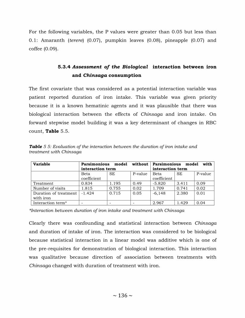
~ 136 ~

For the following variables, the P values were greater than 0.05 but less than

0.1: Amaranth (terere) (0.07), pumpkin leaves (0.08), pineapple (0.07) and

coffee (0.09).

5.3.4 Assessment of the Biological interaction between iron

and Chinsaga consumption

The first covariate that was considered as a potential interaction variable was

patient reported duration of iron intake. This variable was given priority

because it is a known hematinic agents and it was plausible that there was

biological interaction between the effects of Chinsaga and iron intake. On

forward stepwise model building it was a key determinant of changes in RBC

count, Table 5.5.

Table 5 5: Evaluation of the interaction between the duration of iron intake and treatment with Chinsaga

Variable Parsimonious model without

interaction term

Parsimonious model with

interaction term

Beta

coefficient

SE P-value Beta

coefficient

SE P-value

Treatment 0.834 1.195 0.49 -5.820 3.411 0.09

Number of visits 1.815 0.755 0.02 1.709 0.741 0.02

Duration of treatment

with iron

-1.424 0.715 0.05 -6,148 2.380 0.01

Interaction term* - - - 2.967 1.429 0.04

*Interaction between duration of iron intake and treatment with Chinsaga

Clearly there was confounding and statistical interaction between Chinsaga

and duration of intake of iron. The interaction was considered to be biological

because statistical interaction in a linear model was additive which is one of

the pre-requisites for demonstration of biological interaction. This interaction

was qualitative because direction of association between treatments with

Chinsaga changed with duration of treatment with iron.

~ 137 ~

One-way sensitivity analysis was conducted to determine the threshold

duration of iron intake at which Chinsaga began to have a beneficial effect

Table 5.6 . The beta coefficient of the treatment variable was negative if patient

reported duration of iron intake was less than about 1.5 to 2 months.

Table 5 6: One way sensitivity analysis of the effect of patient reported duration of intake of iron supplements on the beta coefficient of the effect of treatment with Chinsaga on RBC

Duration on Iron supplements

(months)

Beta coefficient of the Treatment

variable

>3 83.20

3 3.0820

2 0.115

1 -2.85

0 -5.820

In addition, confounding and interaction with other covariates was explored

and the results are presented in Table 5.7. Analysis was restricted to variables

for which there was a statistical significant association with RBC count on

bivariable analysis.The variables marital status, Ugali, traditional herbs, coffee,

uji displayed collinearity and were therefore dropped.

The only variables that caused at least 10 % change in the crude beta

coefficient of the association between treatment and RBC counts were the use

of bone soup and water melons. The apparent confounding effect of water

melons and avocados was attributed to selection bias because when the

consumption of various foods across arms was conducted more participants in

the Chinsaga arm reported past consumption of water melons (P=0.01) and

avocados (P=0.03) compared to those in the Kale arm. The sample size was

therefore too small to make any conclusive inferences.

It was also difficult to determine whether the effect of soup was due to selection

bias because difference in consumption across arms was almost statistically

~ 138 ~

significant (P=0.08). Consequently patient reported consumption soup seemed

to be only confounder in the association between treatment with Chinsaga and

RBC.

Table 5 7: Evaluation for biological interaction and confounding between Chinsaga and other covariate use

Second variable Coefficient SE P value P-value of interaction

term

Treatment 1.653 0.745 0.03 0.13

Visit 0.828 0.479 0.08

Treatment 1.684 0.749 0.03 collinearity

Herb 12 -8.077 5.005 0.11

Treatment 1.725 0.736 0.02 0.74

Cocoa 1.757 0.736 0.02

Treatment 1.621 0.754 0.03 0.23

Coffee 1.342 1.008 0.18

Treatment 2.108 0.744 0.01 0.05

Soup -1.921 0.753 0.01

Treatment 1.650 0.747 0.03 0.92

Uji (Porridge) -1.353 0.864 0.12

Treatment 1.276 0.817 0.12 0.97

Melon 1.435 0.808 0.08

Treatment 1.916 0.752 0.01 0.16

Black beans (Njahi) 1.499 0.747 0.05

Treatment 1.879 0.690 P<0.01 0.11

Ugali (Maize meal) 9.255 1.669 P<0.01

Treatment 1.890 0.740 0.01 0.13

Amaranth (terere) -1.833 0.921 0.05

Treatment 1.525 0.783 0.05 0.44

Avocado 1.372 0.853 0.11

When the duration of iron consumption was added as the third explanatory to

the models presented in Table 5.7, all other variables lost statistical

significance.

5.4 Discussion

The aim of this study was to establish if there is any improvement of selected

hematological parameters by including Chinsaga in the diet. The key findings

of this study were participants in the arm treated with Chinsaga had

~ 139 ~

statistically significant higher RBC counts on Day 14 and 28 compared to

patients in the Kale treated arm. There was qualitative biological interaction

between patient reported duration of intake of iron supplements and treatment

with Chinsaga and was effective in participants who had taken iron for at least

one month.

For the outcomes, hematocrit and hemoglobin there were no statistically

significant differences across the treatment arms from the baseline to Day 28.

For the rest of the variables (RBC; MCV, RDW, HCTC) changes occurred

between groups.

Looking at the MCHC, it was observed there was a statistically significant

difference across the two arms in the baseline. This difference was reflected in

the sub-population that came for Day 14. On Day 28 there was no statistically

significant difference across the two arms which suggested that one treatment

was curative and improved indices in the arms that systemically had low levels.

Mothers with anemia raise the risk of having complications during pregnancy

and delivery and undesirable pregnancy outcome.

However, it was noted, time of residence in current location was very highly

significance (P<0.01). This suggests that the longer a woman has spent in her

current residence the better her values of RBC count. The question arises then,

what is it about staying in one location that would have a relationship with the

state of a woman’s RBC levels?

Several factors may be involved. It may be speculated that the longer one lives

in an environment, the more likely they are to have overcome initial challenges

which include sourcing of resources and especially where they get affordable

foods. In addition, it may be related to the establishment of networks among

the women that provide social needs that translate into intangible resources

that further support her in such a manner impacting on her health. It may also

~ 140 ~

be true that living in one location for long also enables one identify protective

behavior patterns and minimization of exposure to elements of harm. This may

need to be investigated further.

On bivariable analysis, marital status (P=0.05) and especially age of husband

(P<0.01) were positively associated with RBC counts. Social aspects evidently

have an important contribution to the welfare of the women. These too may be

tied to the benefits of protection and social stability in influencing the health of

women. Sharing the bed with the baby and eating maize meal (Ugali) were also

strongly correlated with RBC count (P<0.01).

Studies have been done on the effects of rooming in on mother and babies in

hospital settings. Evidence shows that rooming in largely benefits the mother

relationship with the baby by allowing more skin contact and easier placing of

the baby on the breast by the mother. However, there is also the indication that

the mothers tend to have less sleep due to a raised consciousness of the baby

losing their depth of sleep as they remain sensitive to turning over the baby.

In the home setting, the mother may have similar challenges as the hospital,

but the factors here are different because of the existence of the father of the

baby on the same bed. Depending on the size of the bed, the baby may be a

source of duress for the mother as she tries to squeeze into the space of the

bed

This then raises the question, what does living in an area for long, having a

more mature husband, sleeping with the baby; eating melon and drinking

cocoa have in common? Are they surrogate indicators of behavior that results

in improved maternal RBC count? If so what are they? Again, this is an

opportunity to conduct further social investigations on the women using these

parameters to determine the common aspects in their environment or behavior

that relates with the RBC count.

~ 141 ~

Surprisingly, education (P=0.90), ethnicity (0.80), occupation (P=0.58), of the

woman and less so the husband (P=0.3) had no statistically significant

association with RBC counts. This was unexpected since these are normally

expected to influence nutritional behavior and consequently hematological

parameters. Education of women is particularly important in health circles in

relation to maternal health outcomes .

Evaluation of the effects of data collected in the study revealed that it is

prudent to include socioeconomic and anthropological factors in the forecast

during interpretation of data especially in a varied society as that found in

Kenya. Results of hemoglobin levels showed much less change over the three

visits as observed in the p value. Hemoglobin is often used as simple measure

of iron status and is widely used for classification of anemia.

The Shapiro Wilk test showed that none of the outcome variables was normally

distributed. Most needed transformation for normality to be achieved. By

evaluating the cumulative results of RDW, correlation was observed with other

parameters. One advantage with the use of this parameter is the ease of

application in rural laboratory settings.

Looking at the treatment groups, the mean Hb value for the Chinsaga group

appeared to increase more steadily than the Kale group where the value seems

to rise and fall back to baseline value within the four weeks. Assuming the

effect is consistent over time, this change in MCHC may yet be the most

sensitive indicating a diminishing difference in the two groups over time.

However, there is also the possibility MCHC may be changing due to a natural

tendency for the body among the women to correct for changes in blood levels

due to losses after delivery. In this case the effect observed in the study would

need to be evaluated in a separate study involving women that are neither

pregnant nor well beyond the initial months post delivery.

~ 142 ~

5.5 Conclusion

Through our present study, the results confiirm that Chinsaga consumption

increases iron uptake during supplementation. It may thereafter be formulated

as an adjunct in iron supplementation to postpartum women. Overall,

additional studies should be carried out to elucidate the mechanism for the

observed effects on RBC count and MCHC and the extent of influence on

cellular markers of iron metabolism.

This study therefore recommends the conduct of similar studies on other

traditional vegetables consumed by various communities in Kenya as a way of

preserving the knowledge and promoting their incorporation into the diet for

the benefit of mankind.

In this clinical trial surrogate makers were used as endpoints. Challenges and

problems faced were in: recruitment and retention, ambiguous situations, time

and resource limitations, laboratory equipment, data management, assessment

of safety and dose response determinations translating this clinical trial into a

proof of concept study.

5.6 Study limitations

Specific methods of diagnosis of iron deficiency such as ferritin levels was not

elucidated in this study but may form a useful adjunct to include in future

investigations of the Chinsaga effects. Dehydration as well as over-hydration

may alter the values of the measurement and were not controlled for in this

study.

~ 143 ~

5.7 References

1. Bothwell TH, Charlton RW, Cook JD, Finch CA. Iron metabolism in man.

Iron Metab Man [Internet]. 1979 [cited 2013 Oct 20]; Available from: http://www.cabdirect.org/abstracts/19801408535.html

2. Miret S, Simpson RJ, McKie AT. Physiology and molecular biology of dietary iron absorption. Annu Rev Nutr. 2003;23(1):283–301.

3. Kemna EH, Tjalsma H, Willems HL, Swinkels DW. Hepcidin: from

discovery to differential diagnosis. Haematologica. 2008;93(1):90–7.

4. World Health O. Diet nutrition and the prevention of chronic diseases Report of a Joint FAO/WHO Expert Consultation. Report of a Joint

FAO/WHO Expert Consultation, WHO, Geneva; 2003. Report No.: Series #916.

5. Stoev S, Dikov I, Iovchev S, Ivanov S. [Hemorheological parameters in the prognosis of the risk of fetal retardation in pregnancy with arterial hypertension]. Akusherstvo Ginekol. 1996;35(4):23–4.

6. Milman N, Agger AO, Nielsen OJ. Iron status markers and serum erythropoietin in 120 mothers and newborn infants: Effect of iron

supplementation in normal pregnancy. Acta Obstet Gynecol Scand. 1994;73(3):200–4.

7. Khoigani MG, Goli S, Hasanzadeh A. The relationship of hemoglobin and

hematocrit in the first and second half of pregnancy with pregnancy outcome. Iran J Nurs Midwifery Res. 2012 Feb;17(2 Suppl 1):S165–70.

8. Ervasti M, Kotisaari S, Heinonen S, Punnonen K. Use of advanced red

blood cell and reticulocyte indices improves the accuracy in diagnosing iron deficiency in pregnant women at term. Eur J Haematol.

2007;79(6):539–45.

9. Krafft A, Perewusnyk G, Hänseler E, Quack K, Huch R, Breymann C. Effect of postpartum iron supplementation on red cell and iron

parameters in non-anaemic iron-deficient women: a randomised placebo-controlled study. BJOG Int J Obstet Gynaecol. 2005;112(4):445–50.

10. Allen LH. Pregnancy and Iron Deficiency: Unresolved Issues. Nutr Rev. 1997;55(4):91–101.

11. Adu-Afarwuah S, Lartey A, Brown KH, Zlotkin S, Briend A, Dewey KG.

Home fortification of complementary foods with micronutrient

~ 144 ~

supplements is well accepted and has positive effects on infant iron status in Ghana. Am J Clin Nutr. 2008;87(4):929–38.

12. Milman N, Bergholt T, Byg K-E, Eriksen L, Graudal N. Iron status and iron balance during pregnancy. A critical reappraisal of iron

supplementation. Acta Obstet Gynecol Scand. 1999;78(9):749–57.

13. Tamura T, Goldenberg RL, Hou J, Johnston KE, Cliver SP, Ramey SL, et al. Cord serum ferritin concentrations and mental and psychomotor

development of children at five years of age. Obstet Gynecol Surv. 2002;57(8):493–4.

14. Trugo NM. Micronutrient regulation in pregnant and lactating women

from Rio de Janeiro. Arch Latinoam Nutr. 1997 Jun;47(2 Suppl 1):30–4.

15. Kaltwasser JP, Werner E, Niechzial M. Bioavailability and therapeutic

efficacy of bivalent and trivalent iron preparations. Arzneimittelforschung. 1987;37(1A):122.

16. Mehta BC. Failure of oral iron therapy in treatment of iron deficiency

anemia: pharmaceutical iatrogenic cause. Indian J Med Sci. 2001;55(3):157.

17. Ruiz-Argüelles GJ, Díaz-Hernández A, Manzano C, Ruiz-Delgado GJ. Ineffectiveness of oral iron hydroxide polymaltose in iron-deficiency anemia. Hematology. 2007;12(3):255–6.

18. Nielsen P, Gabbe EE, Fischer R, Heinrich HC. Bioavailability of iron from oral ferric polymaltose in humans. Arzneimittelforschung. 1994;44(6):743–8.

19. Ettyang GA, van Marken Lichtenbelt WD, Esamai F, Saris WHM, Westerterp KR. Assessment of Body Composition and Breast Milk Volume

in Lactating Mothers in Pastoral Communities in Pokot, Kenya, Using Deuterium Oxide. Ann Nutr Metab. 2005;49(2):110–7.

20. Keverenge-Ettyang GA, van Marken Lichtenbelt W, Esamai F, Saris W.

Maternal nutritional status in pastoral versus farming communities of West Pokot, Kenya: differences in iron and vitamin A status and body composition. Food Nutr Bull. 2006 Sep;27(3):228–35.

21. Yang JM, Wang KG. Relationship between acute fetal distress and maternal-placental-fetal circulations in severe preeclampsia. Acta Obstet

Gynecol Scand. 1995 Jul;74(6):419–24.

22. Karita E, Ketter N, Price MA, Kayitenkore K, Kaleebu P, Nanvubya A, et al. CLSI-Derived Hematology and Biochemistry Reference Intervals for

~ 145 ~

Healthy Adults in Eastern and Southern Africa. PLoS ONE. 2009 Feb 6;4(2):e4401.

23. Schulz KF, Grimes DA. Generation of allocation sequences in randomised trials: chance, not choice. The Lancet. 2002;359(9305):515–9.

24. Schulz KF, Grimes DA. The Lancet handbook of essential concepts in clinical research [Internet]. Elsevier London; 2006 [cited 2013 Sep 8]. Available from:

http://www.lavoisier.fr/livre/notice.asp?id=OOSWOKAKSXXOWK

~ 146 ~

CHAPTER SIX

6.0 Effects of Chinsaga on Biomarkers of Iron

Metabolism in Serum and Breast milk

~ 147 ~

6.1 Introduction and background

Gynandropsis gynandra (Chinsaga) is a rich source of beta carotene ( a pro-

vitamin A),with its content, ranging between 6.7 -18.9 g per 100 g of vegetable

(1). Vitamin A supplementation has an effect on iron metabolism. Bloem et al

demonstrated that biochemical indicators of Vitamin A status including retinol

and retinol-binding protein correlated with biomarkers of iron metabolism such

as serum Iron and percentage saturation of transferrin (%ST). However, this

difference in retinol, retinol-binding protein, serum Fe, and % Saturation of

Transferrin (%ST) diminished after 4 months (2).

6.1.1 Biomarkers of Iron Metabolism

According to the National Cancer Institute in America, the term biomarker

refers to: “a biological molecule found in blood, other body fluids, or tissues

that are a sign of a normal or abnormal process or of a condition or disease. A

biomarker may be used to see how well the body responds to a treatment for a

disease or condition. Biomarkers are also called molecular marker and

signature molecule”(3). The US National Institutes of Health defines a

biomarker as “a characteristic that is objectively measured and evaluated as an

indicator of normal biological processes, pathogenic processes, or

pharmacologic responses to a therapeutic intervention”(4) .

Biomarkers can therefore be viewed as tools to improve understanding about

diseases and process from initial to the final state. They may help monitor

progression and management of diseases. Depending on the focus,

biomolecules as biomarkers can be classified into: (i) Genomic biomarkers:

based on the analysis of DNA (deoxyribonucleic acid), (ii) Transcriptomic

biomarkers: based on the analysis of RNA expression profiles, (iii) Proteomic

biomarkers: based on the analysis of the protein profiles and (iv) Metabolomic

biomarkers: based on the analysis of metabolites. Alternatively, certain

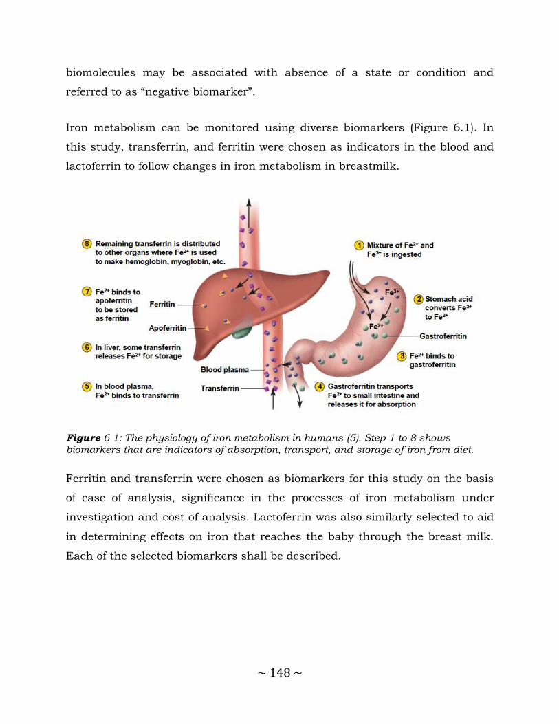
~ 148 ~

biomolecules may be associated with absence of a state or condition and

referred to as “negative biomarker”.

Iron metabolism can be monitored using diverse biomarkers (Figure 6.1). In

this study, transferrin, and ferritin were chosen as indicators in the blood and

lactoferrin to follow changes in iron metabolism in breastmilk.

Figure 6 1: The physiology of iron metabolism in humans (5). Step 1 to 8 shows biomarkers that are indicators of absorption, transport, and storage of iron from diet.

Ferritin and transferrin were chosen as biomarkers for this study on the basis

of ease of analysis, significance in the processes of iron metabolism under

investigation and cost of analysis. Lactoferrin was also similarly selected to aid

in determining effects on iron that reaches the baby through the breast milk.

Each of the selected biomarkers shall be described.

~ 149 ~

6.1.2 Transferrin

Human transferrin is a serum glycoprotein of about 80 kDA which complexes

iron, and transports it through the circulatory system. In people with low iron

levels, more transferrin is produced by the liver this is thought to be a

compensatory reaction, to make more iron available to the body, including the

brain. Iron deficiency alters dopamine metabolism in the caudate and

putamen. People with high transferrin and lower brain iron might have lower

volumes of dopamine containing structures, involved in learning and motor

control (6).

In humans, for example, increased serum transferrin is associated with dietary

iron deficiency and pregnancy (7). Experimental studies in murine models (8)

have suggested that nutritional iron deficiency, thyroxin, glucocorticoids, and

estrogen all cause an increase in serum transferrin specifically inducing an

increase in the rate of liver transferrin synthesis.

Neither the physiological significance of these changes in serum transferrin nor

the mechanism by which the liver responds to hormones and nutritional

stimuli is fully understood. Elevated transferrin levels are associated with an

increase in iron absorption and mobilization of iron from tissue stores,

although the role of transferrin in these changes is unclear. The response to

hormones, such as estrogen, may be important during pregnancy when the

demand for iron by the fetus is high; transferrin specifically releases iron to the

placenta and the increase in circulating transferrin may facilitate this process

(9).

The liver is the main site of transferrin synthesis, but other tissues and organs,

such as the brain, also produce it. The main role of transferrin is to deliver iron

from absorption centers in the duodenum and white blood cell macrophages to

all tissues. Transferrin plays a key role where erythropoiesis and active cell

~ 150 ~

division occur (10). The transferrin receptor helps maintain iron homeostasis in

the cells by controlling iron concentrations.

Transferrin is also associated with the innate immune system. It is found in the

gut mucosa and binds iron, thus creating an environment low in free iron that

impedes bacterial survival in a process called iron withholding. The level of

transferrin decreases in inflammation (11).

Transferrin imbalance can have serious health effects for those with low or

high serum transferrin levels. A patient with an increased serum transferrin

level often suffers from iron deficiency anemia (10). A patient with decreased

plasma transferrin can suffer from iron overload diseases and protein

malnutrition. An absence of transferrin results from a rare genetic disorder

known as atransferrinemia; a condition characterized by anemia and

hemosiderosis in the heart and liver that leads to complications, including

heart failure. Most recently, transferrin and its receptor have been shown to

diminish tumor cells by using the receptor to attract antibodies (12).

Serum transferrin plays a vital role in the transport of iron from intestinal

absorption sites and sites of storage (primarily liver, spleen, and bone marrow),

to reticulocytes where the iron is incorporated into hemoglobin. Transferrin is

synthesized primarily in the liver, although synthesis has also been detected in

the spleen and bone marrow (13). The circulating concentration of serum

transferrin ranges from 1 to 2.5 mg/ml in mammals and birds; however, this

level is regulated by a variety of hormones and nutritional factors.

6.1.3 Ferritin

Ferritin is the major intracellular iron storage protein in all cells. It is

composed of 24 subunits of the heavy and light ferritin chains. Variation in

ferritin subunit composition may affect the rates of iron uptake and release in

~ 151 ~

different tissues. A major function of ferritin is the storage of iron in a soluble

and nontoxic state. Defects in this light chain ferritin gene are associated with

several neurodegenerative diseases and hyperferritinemia-cataract syndrome.

This gene has multiple pseudogenes (14).

Increasingly, perturbations in cellular iron and ferritin are emerging as an

important element in the pathogenesis of disease. These changes in ferritin are

important not only in the classic diseases of iron acquisition, transport, and

storage, such as primary hemochromatosis, but also in diseases characterized

by inflammation, infection, injury, and repair. Among these are some of the

most common diseases that afflict mankind: neurodegenerative diseases such

as Parkinson disease and Alzheimer disease, vascular diseases such as cardiac

and neuronal ischemia-reperfusion injury, atherosclerosis itself, pulmonary

inflammatory states, rheumatoid arthritis, and a variety of premalignant

conditions and frank cancers (15).

The link between alteration in ferritin regulation and these diseases is forged

through a diverse set of cellular stress pathways that alter ferritin subunit

composition and/or content within cells (16).

Ferritin sequesters iron in a nontoxic form, but levels of “labile” iron regulate

cellular ferritin levels, protecting cells from damage triggered by excess iron.

Iron-mediated, largely posttranscriptional pathways of ferritin regulation have

been identified through a series of elegant experiments over the last 15 years

(17–19).

The content of cytoplasmic ferritin is regulated by the translation of ferritin H

and L mRNAs in response to an intracellular pool of “chelatable” or “labile” iron

(20,21). Thus, when iron levels are low, ferritin synthesis is decreased;

conversely, when iron levels are high, ferritin synthesis increases. Although in

certain circumstances there is an increase in ferritin mRNA in response to iron,

~ 152 ~

(22) the regulatory response of ferritin to iron is largely posttranscriptional, (23)

and is due to the recruitment of stored mRNA from monosomes to polysomes in

the presence of iron (21).

This process is mediated by interaction between RNA binding proteins and a

region in the 5′ untranslated region of ferritin H and L mRNA termed the iron

responsive element (IRE) that has a “stem-loop” secondary structure. There are

2 RNA binding proteins, iron regulatory proteins 1 and 2 (IRP1 and IRP2), that

bind to this stem loop structure and inhibit mRNA translation. However, the

proteins are regulated differently: IRP1 is an iron-sulfur cluster protein that

exists in 2 forms. When iron is abundant, it exists as a cytosolic aconitase.

When iron is scarce, it assumes an open configuration associated with the loss

of iron atoms in the iron-sulfur cluster, and can bind the IRE stem loop, acting

as a repressor of ferritin translation. In contrast, IRP2 is regulated by

degradation: IRP2 protein is abundant in iron scarcity, but is degraded rapidly

in iron excess through targeting of a unique 73 amino acid sequence (24).

Although both IRP1 and IRP2 bind the IRE and exert an inhibitory effect on

ferritin synthesis, there is evidence that IRP1 and IRP2 may have distinct

tissue-specific roles (25).

IRE-IRP binding lengthens transferrin receptor mRNA half-life, ultimately lead

to increased transferrin receptor display on the cell surface in situations of iron

depletion (26). Thus, similar RNA-protein binding motifs can have strikingly

different biologic effects when located in different positions on different genes.

In the case of ferritin, IRP binding results in inhibition of translation, whereas

in the transferrin receptor, IRP binding increases transferrin receptor mRNA

half-life (26).Transcription of the human ferritin H gene is induced in response

to both hormones and second messengers, including cAMP. The cis-acting

elements mediating these responses have mapped to a relatively small region in

the proximal promoter of the human ferritin H gene (27).

~ 153 ~

Thyroid hormone may also regulate ferritin posttranscriptionally: T3 modulates

the activity of IRP1, affecting its ability to bind to the ferritin IRE, possibly

through induction of signal transduction cascades that result in

phosphorylation of IRP1 (28). T3 and TRH also induce the phosphorylation of

IRP2 (29).

In addition, the shorter circulation time for reticulocytes of one to two days

means the changes in Reticulate Haemoglobin Content (CHr) and percentage of

hypochromic red blood cells (%HYPOm) is more responsive to changes in

availability of iron for erythropoiesis. However, those based on red blood cell

with a lifespan of 120 days are the established markers of iron status over the

longer duration (30).

It is worth noting that the various parameters reflect different aspects of iron

deficiency. While cellular indices reflect iron deficient erythropoiesis,

biochemical markers reflect iron availability for erythropoiesis (TfR), iron stores

(ferritin), or circulating iron bound to transferrin (TfSat). It is known that iron

and transferrin have biological variability, and ferritin reacts as an acute phase

reactant (31). However, %HYPOm has been shown to be unaffected by

physiologic inflammatory processes in the postpartum period(32).

Consistent with earlier studies (33), the mean value of ferritin was low in

pregnant women at term, yet only a few with low ferritin had produced iron

deficient erythrocytes. Therefore, it is likely that the reduction in serum ferritin

does not exclusively reflect exhausting iron stores. The increase in TfR

concentration during pregnancy is assumed to be a consequence of accelerated

erythropoiesis (34), which makes it difficult to judge whether an elevated

concentration is due to an increased demand for iron or an enhanced rate of

erythropoiesis.

~ 154 ~

6.1.4 Lactoferrin

Lactoferrin, a non-haem iron-binding glycoprotein, is mainly found in milk. It is

a major protein in the secondary granules of neutrophils and is present in

many biological secretions including the saliva, tears and semen. The protein

has been shown to kill bacteria, play an immunomodulatory role and

participate in inflammatory response (35–37). However, its mechanism of

action is presently unknown. Lactoferrin expression is up-regulated by both

estrogens and epidermal growth factor (EGF) (38).

Estrogen regulation of lactoferrin gene expression in the uterus is well

established (38). However, there are inconsistent reports on estrogen regulation

of the lactoferrin gene in human endometrium (39–42). Estrogen receptor binds

to the imperfect ERE of human lactoferrin gene both in isolation and in the

context of the gene promoter region. Human lactoferrin gene is activated in

transiently transfected human endometrial carcinoma cells through an ER-

mediated process and that the imperfect ERE of the gene is required (40). In

addition to the in vitro physical interaction between ER and the ERE of the

human lactoferrin gene, lactoferrin gene expression in the endometrium

fluctuates during the menstrual cycle. In Western blotting experiments,

lactoferrin has been detected in the proliferative phase but not in the secretory

phase, suggesting that estrogen induces and progesterone suppresses

lactoferrin gene expression in vivo. This provides a relatively homogeneous cell

population.

The lactoferrin of rhesus monkey has high similarity to the human protein in

both amino acid composition and carbohydrate moiety (43). Moreover, monkey

lactoferrin, like human lactoferrin, has an unusual amino acid sequence at the

N-terminus which is essential for binding to bacterial lipopolysaccharide and to

the mammalian lactoferrin receptor (37,44), indicating that monkey lactoferrin

could function similarly to the human protein. The reproductive physiology of

~ 155 ~

the female rhesus macaque monkey is also highly comparable to that of women

(43). However, the polyclonal antibody produced against human lactoferrin

does not cross-react with the monkey milk lactoferrin nor does it detect any

immuno-reactive protein in the endometrial tissue.

Little is known about the factors that influence milk lactoferrin levels, although

it is known that concentration decreases during lactation (36), Zavaleta et al,

(45) found the concentration of lactoferrin had decreased by day 30 of

breastfeeding. In a study by Fransson et al. (1985) (46) , lactoferrin levels were

found to be high in severely anemic women; however, the number of subjects

was very low. Houghton et al, (46) studied lactoferrin levels in Aborigine women

in Australia and found lower levels in milk from women with poor nutritional

status than in milk for well nourished women.

6.1.5 Objectives

This study sought to determine the effect of Chinsaga consumption on

biomarkers of iron metabolism ferritin and transferrin in serum and lactoferrin

in breastmilk over a 28 day period.

6.1.6 Specific Objectives

1. To establish the effect of Chinsaga treatment on expression of the Transferrin gene in plasma

2. To establish the effect Chinsaga consumption on expression of the Ferritin

gene in plasma

3. To establish the effect Chinsaga consumption on expression of Lactoferrin

gene in breast milk

~ 156 ~


Blood samples of about 4 ml were drawn from the antecubetal vein using a

needle 21G and syringe at each visit from each volunteer from Chinsaga group

and control group. The blood was then emptied into EDTA tubes (Beckton

Dickinson, Germany) and delivered to the hematology laboratory at KAVI. This

was done at baseline and during the follow up after delivery. As long as the

mother was willing to participate and was breast-feeding, blood samples were

taken at midmorning (9: 00 to 11:00 AM) during the clinic visits (day 0, 14 and

28). The samples were used to run full haemogram after which the serum was

separated. The serum obtained was then divided into two aliquotes for storage

at -70 C in serum vials until the time of analysis.

6.2.1 Extraction of transferrin mRNA

Human serum, 50µl, was drawn into a 1.5ml eppendorf tube. Lysis buffer,

100µl, was then added and incubated at 37⁰C for 30 minutes in a thermomixer

shaking at 1000rpm. The lysates were homogenized by vortexing briefly. Flow

was applied through the RNeasy column, it was then subjected to two washes

with the first wash using 100µl of wash buffer I and the second wash using

200µl of wash buffer II. 50µl of RNA was eluted in RNA free water. RNA, 10µl,

was subjected to DNaseI digestion by adding 1µl of DNaseI then 1µl of DNase

inhibitor.

6.2.2 Synthesis of transferrin cDNA

A master mix containing 1µl random primers, 1µl annealing buffer, 10µl RNase

free water and 3µl of the sample RNA. This mixture was incubated in a

thermocycler machine (BioRad, UK) at 65⁰C for 5 minutes then immediately

placed on ice for 1 minute. The contents of the tube were then centrifuged

briefly. The 2X first strand reaction mixture containing 10µl superscript III

~ 157 ~

were then added. RNase out enzyme, 2µl, was then added. The sample mixture

was then incubated at 50⁰C for 50 minutes, then 25⁰C for 10 minutes and

finally 50⁰C for 50 minutes. The reaction was terminated by incubating the

mixture at 85⁰C for 5 minutes. Amplification reaction mixes consisted of 1–

1000 ng of template DNA, 0.5 IU of thermostable DNA polymerase, 0.2 mmol/l

dNTPs, 1.5–3.0 mmol/l magnesium chloride, 10–30 pmoles of primers and PCR

reaction buffer (20 mmol/l Tris–HCl, pH 8.4 and 50 mM KCl), in a final volume

of 20 μl. All samples were initially denatured at 95°C for 5 min followed by 30

cycles of 95°C for 1 min, 50°C for 2 min and 72°C for 3 min. A final extension

step of 72°C for 5 min was included. All PCR reactions were performed on a

pre-programmed automated DNA thermal cycler (BioRad, UK). Using primers

with TF1 5’ GGG TGG AACT ATACT CCACTG ATG GG 3’as the forward primer

and TF2 5’AAA GCGC CCAT GTGA TAGA CC 3’ a 419 bp fragment of the

transferrin gene from human serum RNA was amplified (47).

6.2.3 Results of gel electrophoresis of transferritin

Nested PCR product, five microlitres, was mixed with a 1-2 µl of 10× loading

dye and analyzed by agarose gel electrophoresis on 0.8% agarose gel stained

with Ethidium bromide (0.5 µg/ml) in Tris-acetate-EDTA buffer. The

electrophoresis was run at 80 volts for 30 minutes. DNA was visualized by

ultraviolet transillumination.

The Figure 6.2 is an example of a typical gel after development and

photography of the results from electrophoresis of the transferrin gene

enhanced through PCR. Volunteer numbers are indicated on top of the image.

~ 158 ~

Figure 6 2: Gel after development and visualization of amplified Transferrin genes from human blood using a transilluminator (an ultraviolet lightbox), showing ethidium bromide-stained DNA in gels as bright glowing bands.

6.2.3.1 Analysis of Transferrin Gene

Tranferrin gene during baseline, table 6.1 at the beginning of a one month

period of using Chinsaga in the diet, was generally weakly expressed with the

mean being 2.02 at 95% confidence interval of between 3.77 and 0.266 (Table

6.1 below). Out of the 113 patients whose serum tranferrin levels were

analysed, 39 (34.5%) showed no expression, 36 (31.9%) had weak expression of

the tranferrin gene, 35 (31.0%) had normal gene expression while 3 (2.6%)

showed over expression of the gene. Levels of expression were categorized as

none, weakly expressed, normally expressed and over expressed against an

intensity scale.

~ 159 ~

Table 6 1: Percentage change in the average gene expression of Transferrin as

determined by PCR cDNA template amplification at baseline

Level of tranferrin gene expressed at baseline

Frequency Percentage Cummulative Percentage

None (1) 39 34.5 34.5 Weakly Expressed (2) 36 31.8 66.3 Normally Expressed (3) 35 31.0 97.3

Over Expressed (4) 3 2.7 100 TOTAL 113 100

During the day 14 of using Chinsaga, 44 samples were analysed for transferrin

expression, Table 6.2, most of the patients did not turn up for the follow up

even after making effort in persuing them. There was a slight increase in the

level of tranferrin gene expression at a mean of 2.25 and 95% confidence

interval. The confidence interval ranges from 4.23 to 0.267. Out of the 44

samples analysed, 14 (31.8%) showed no expression, 8 (18.2%) had weak

expression of the tranferrin gene, 18 (43.2%) had normal gene expression while

3 (6.8%) showed over expression of the gene.

On Day 28, of using Chinsaga in the diet, 33 samples were analysed for

transferrin expression, Table 6.3 and Figure 6.2, some patients did not turn

up for the follow up even after making every effort to persue them. Again a

slight increase in the level of tranferrin gene expression was observed at a

mean of 2.3 and 95% confidence level. The confidence interval ranges from

4.49 to 0.170. Out of the 33 samples analyzed, 10 (30.3%) showed no

expression, 7 (21.2%) had weak expression of the transferrin gene, 11 (33.3%)

had normal gene expression while 5 (15.2%) showed over expression of the

gene (Figure 6.3). The difference was statistically significant with analysis

using the F40 -test gaving a value of 2.6, a p value of 0.00669. The calculated

F40 at 95% confidence level test is greater than the tabulated value which is

1.91.

~ 160 ~

Table 6 2: Percentage change in the average gene expression of transferrin as determined by PCR cDNA template amplification on Day 14.

Level of tranferrin gene expressed at Day 14

Frequency Percentage Cummulative Percentage

None (1) 14 31.8 31.8 Weakly Expressed (2) 8 18.2 50.0

Normally Expressed (3) 19 43.2 93.2 Over Expressed (4) 3 6.8 100 TOTAL 44 100

Table 6 3: Percentage change in the average gene expression of transferrin as determined by PCR coda template amplification in visit three

Level of transferrin gene expressed at Day 28

Frequency Percentage Cumulative Percentage

None (1) 10 30.3 30.3

Weakly Expressed (2) 7 21.2 51.5 Normally Expressed (3) 11 33.3 84.8 Over Expressed (4) 5 15.2 100

TOTAL 33 100

Figure 6 3: Change in the average Transferrin gene expression on days; 0,14 and 28 as determined by PCR cDNA template amplification.

~ 161 ~

6.2.4 Extraction of ferritin mRNA

Human serum, 50µl, was drawn into a 1.5ml eppendorf tube. Lyses buffer,

100µl, was then added and incubated at 37⁰C for 30 minutes in a thermomixer

shaking at 1000rpm. The lysates were homogenized by vortexing briefly. Flow

was applied through the RNeasy column, it was then subjected to two washes

with the first wash using 100µl of wash buffer I and the second wash using

200µl of wash buffer II. 50µl of RNA was eluted in RNA free water. RNA, 10µl,

was subjected to DNaseI digestion by adding 1µl of DNaseI then 1µl of DNase

inhibitor.

6.2.4.1 Synthesis of ferritin cDNA


free water and 3µl of the sample RNA was incubated in a thermocycler machine

(BioRad, UK) at 65⁰C for 5 minutes then immediately placed on ice for 1

minute. The contents of the tube were then centrifuged briefly. The 2X first

strand reaction mixture containing 10µl superscript III were then added. 2µl

RNase out enzyme was then added. The sample mixture was then incubated at

50⁰C for 50 minutes, then 25⁰C for 10 minutes and finally 50⁰C for 50

minutes. The reaction was terminated by incubating the mixture at 85⁰C for 5

minutes. Amplification reaction mixes consisted of 1–1000 ng of template DNA,

0.5 IU of thermostable DNA polymerase, 0.2 mmol/l dNTPs, 1.5–3.0 mmol/l

magnesium chloride, 10–30 pmoles of primers and PCR reaction buffer (20

mmol/l Tris–HCl, pH 8.4 and 50 mM KCl), in a final volume of 20 μl. All

samples were initially denatured at 94°C for 5 min followed by 30 cycles of

94°C for 1 min, 53°C for 2 min and 65°C for 3 min. A final extension step of

65°C for 6 min was included. All PCR reactions were performed on a pre-

programmed automated DNA thermal cycler (BioRad, UK). Using primers with

FT1 5’ATGAGCTCCCAGATTCGT 3’as the forward primer and FT2

~ 162 ~

5’TTAGTCGTGTTGAGAGTGAG 3’ a 431 bp fragment of the ferritin gene from

human serum RNA was amplified (18).

6.2.4.2 Gel Electrophoresis of PCR results of Ferritin

expression

Five microlitres of nested PCR product was mixed with a 1-2 µl of 10× loading




ultraviolet transillumination.

The Figure 6.4 is an example of a typical gel after development and

photography of the results from electrophoresis of the ferritin gene enhanced

through PCR.

BF1

49V

1

BF1

48

V1

BF1

47V

1

BF1

46V

1

BF1

45

V1

BF1

44V

1

BF1

43V

1

BF1

42V

1

BF1

40V

1

BF1

39V

1

BF1

34V

1

Figure 6 4: Gel of amplified Ferritin genes from human blood using a transilluminator (an ultraviolet light box). Ethidium bromide-stained DNA in gels seen as bright glowing bands.

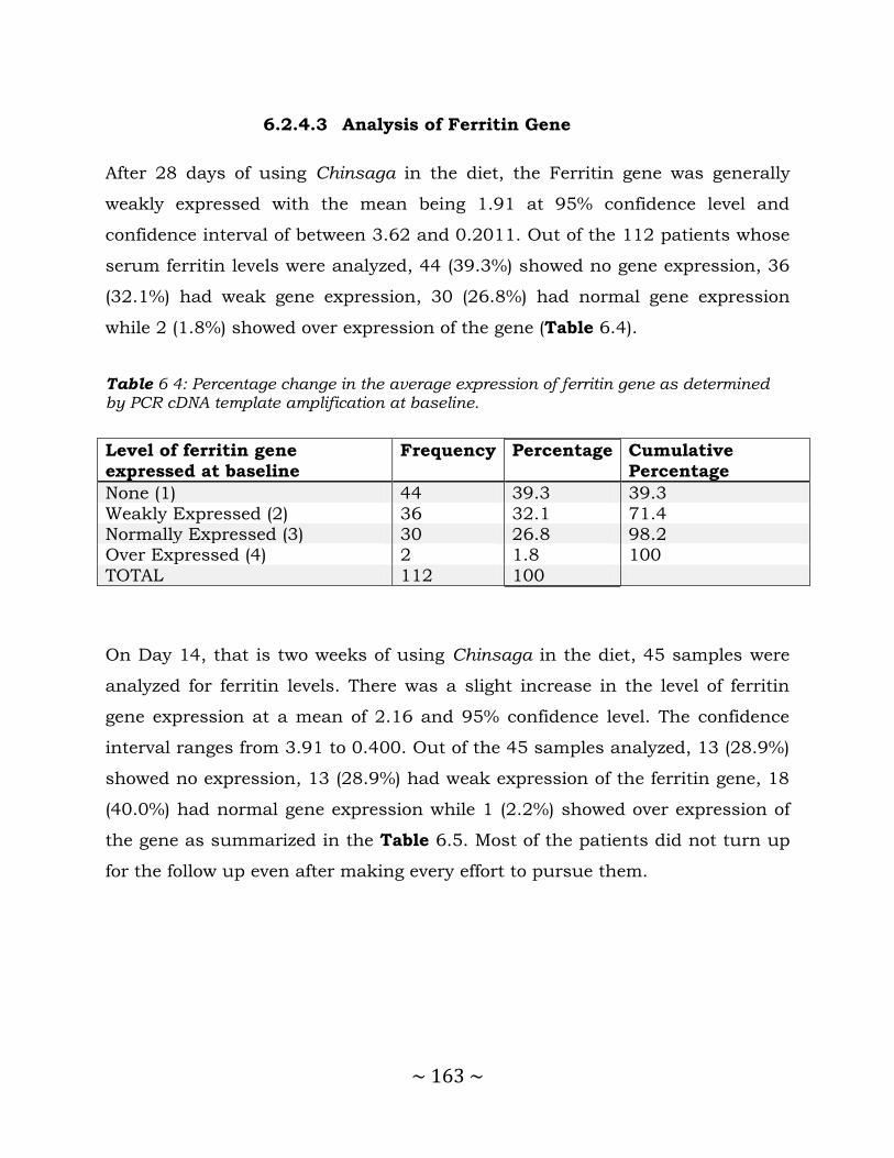
~ 163 ~

6.2.4.3 Analysis of Ferritin Gene

After 28 days of using Chinsaga in the diet, the Ferritin gene was generally

weakly expressed with the mean being 1.91 at 95% confidence level and

confidence interval of between 3.62 and 0.2011. Out of the 112 patients whose

serum ferritin levels were analyzed, 44 (39.3%) showed no gene expression, 36

(32.1%) had weak gene expression, 30 (26.8%) had normal gene expression

while 2 (1.8%) showed over expression of the gene (Table 6.4).

Table 6 4: Percentage change in the average expression of ferritin gene as determined by PCR cDNA template amplification at baseline.

Level of ferritin gene

expressed at baseline

Frequency Percentage Cumulative

Percentage

None (1) 44 39.3 39.3


TOTAL 112 100

On Day 14, that is two weeks of using Chinsaga in the diet, 45 samples were

analyzed for ferritin levels. There was a slight increase in the level of ferritin

gene expression at a mean of 2.16 and 95% confidence level. The confidence

interval ranges from 3.91 to 0.400. Out of the 45 samples analyzed, 13 (28.9%)

showed no expression, 13 (28.9%) had weak expression of the ferritin gene, 18

(40.0%) had normal gene expression while 1 (2.2%) showed over expression of

the gene as summarized in the Table 6.5. Most of the patients did not turn up

for the follow up even after making every effort to pursue them.

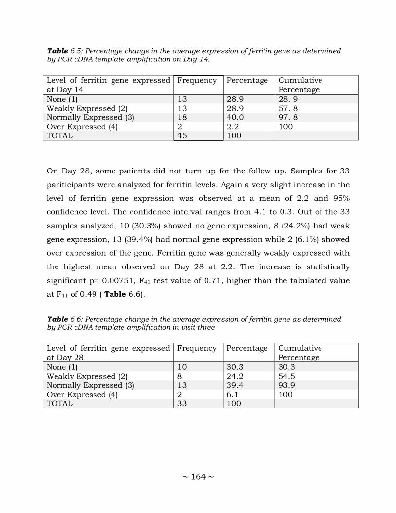
~ 164 ~

Table 6 5: Percentage change in the average expression of ferritin gene as determined by PCR cDNA template amplification on Day 14.

Level of ferritin gene expressed at Day 14


None (1) 13 28.9 28. 9 Weakly Expressed (2) 13 28.9 57. 8 Normally Expressed (3) 18 40.0 97. 8


On Day 28, some patients did not turn up for the follow up. Samples for 33

pariticipants were analyzed for ferritin levels. Again a very slight increase in the

level of ferritin gene expression was observed at a mean of 2.2 and 95%

confidence level. The confidence interval ranges from 4.1 to 0.3. Out of the 33

samples analyzed, 10 (30.3%) showed no gene expression, 8 (24.2%) had weak

gene expression, 13 (39.4%) had normal gene expression while 2 (6.1%) showed

over expression of the gene. Ferritin gene was generally weakly expressed with

the highest mean observed on Day 28 at 2.2. The increase is statistically

significant p= 0.00751, F41 test value of 0.71, higher than the tabulated value

at F41 of 0.49 ( Table 6.6).

Table 6 6: Percentage change in the average expression of ferritin gene as determined by PCR cDNA template amplification in visit three

Level of ferritin gene expressed

at Day 28


Percentage

None (1) 10 30.3 30.3


TOTAL 33 100

~ 165 ~

Figure 6 5: Change in the average Ferritin gene expression days; 0,14, and 28 as determined by PCR cDNA template amplification..

6.2.5 Profiling for Lactoferrin expression in breast milk

Milk samples were obtained from 10 participants in the control group (Kale)

and 10 from the Chinsaga group selected randomly after delivery. As long as

the mother was willing to participate and was breast-feeding, 10 ml milk

samples were taken from each mother at midmorning feeding (9: 00 to 11:00

AM) during the clinic visits (day 0, 14 and 28). This sampling technique has

been proved to be adequate for water-soluble components such as total protein,

non-protein nitrogen, individual proteins, and lactose (48). Hand expression

was used for collection of milk specimens. The samples were pooled and stored

at -20 C until the time of analysis. All analyses were performed on defatted

milk collected on days; 0, 14 and 28 after delivery as previously reported (49)

(50).

6.2.5.1 Extraction of lactoferrin mRNA

Human breast milk (100µl), was drawn into a 1.5ml eppendorf tube. Lysis

buffer, 200µl, was then added and incubated at 37⁰C for 30 minutes in a

~ 166 ~

thermomixer shaking at 1000rpm. The lysates were homogenized by vortexing

briefly. Flow was applied through the RNeasy column, it was then subjected to

two washes with the first wash using 200µl of wash buffer I and the second

wash using 400µl of wash buffer II. RNA, 100µl, was eluted in RNA free water.

Of the RNA, 20µl, was subjected to DNaseI digestion by adding 1µl of DNaseI

then 1µl of DNase inhibitor.

6.2.5.2 Synthesis of lactoferrin cDNA


free water and 3µl of the sample RNA was incubated in a thermocycler machine

(BioRad, UK) at 65⁰C for 5 minutes then immediately placed on ice for 1

minute. The contents of the tube were then centrifuged briefly. The 2X first

strand reaction mixture containing 10µl superscript III was then added. RNase

out enzyme, 2µl, was then added. The sample mixture was then incubated at

50⁰C for 50 minutes, then 25⁰C for 10 minutes and finally 50⁰C for 50

minutes. The reaction was terminated by incubating the mixture at 85⁰C for 5

minutes. Amplification reaction mixes consisted of 1–1000 ng of template DNA,

0.5 IU of thermostable DNA polymerase, 0.2 mmol/l dNTPs, 1.5–3.0 mmol/l

magnesium chloride, 10–30 pmoles of primers and PCR reaction buffer (20

mmol/l Tris–HCl, pH 8.4 and 50 mM KCl), in a final volume of 20 μl. All

samples were initially denatured at 94°C for 5 min followed by 35 cycles of

94°C for 1 min, 50°C for 2 min and 65°C for 3 min. A final extension step of

65°C for 3 min was included. All PCR reactions were performed on a pre-

programmed automated DNA thermal cycler (BioRad, UK). Using primers with

LF1 5’AGGAGGATGCCATCTGGAAT 3’as the forward primer and LF2

5’AACCCAATGGCAGAGTCCTT 3’ a 398 bp fragment of the lactoferrin gene

from human breast milk RNA was amplified (45).

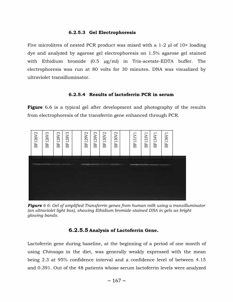
~ 167 ~

6.2.5.3 Gel Electrophoresis

Five microlitres of nested PCR product was mixed with a 1-2 µl of 10× loading




ultraviolet transilluminator.

6.2.5.4 Results of lactoferrin PCR in serum

Figure 6.6 is a typical gel after development and photography of the results

from electrophoresis of the transferrin gene enhanced through PCR.

BF

126V

2

BF

126V

3

BF

128V

3

BF

128V

3

BF

129V

2

BF

129V

3

BF

130V

2

BF

130V

2

BF

131V

1

BF

133V

1

BF

134V

1

BF

136V

1

Figure 6 6: Gel of amplified Transferrin genes from human milk using a transilluminator (an ultraviolet light box), showing Ethidium bromide-stained DNA in gels as bright glowing bands.

6.2.5.5 Analysis of Lactoferrin Gene.

Lactoferrin gene during baseline, at the beginning of a period of one month of

using Chinsaga in the diet, was generally weakly expressed with the mean

being 2.3 at 95% confidence interval and a confidence level of between 4.15

and 0.391. Out of the 48 patients whose serum lactoferrin levels were analyzed

~ 168 ~

14 (29.2 %) showed no expression, 9 (18.8 %) had weak expression of the

lactoferrin gene, 23 (47.9 %) had normal gene expression while 2 (4.2 %)

showed over expression of the gene as shown in the Table 6.7.

Table 6 7: Percentage change in the average gene expression of lactoferrin as determined by PCR cDNA template amplification at baseline

Level of lactoferrin gene expressed at baseline


None (1) 14 29.2 29.2 Weakly Expressed (2) 9 18.7 47.9

Normally Expressed (3) 23 47.9 95.8 Over Expressed (4) 2 4.1 100 TOTAL 48 100

On Day 14 of using Chinsaga in the diet, 51 samples were analyzed for

lactoferrin levels. There was a slight decrease in the level of lactoferrin gene

expression at a mean of 2.2 and 95% confidence level. The confidence interval

ranges from 4.0 to 0.5. Out of the 51 samples analyzed, 13 (25.5%) showed no

expression, 14 (27.4%) had weak expression of the lactoferrin gene, 22 (43.1%)

had normal gene expression while 2 (3.9%) showed over expression of the gene,

Table 6.8.

Table 6 8: Percentage change in the average gene expression of lactoferrin as determined by PCR cDNA template amplification on Day 14.

Level of lactoferrin gene expressed at Day 14


None (1) 13 28.9 28.9 Weakly Expressed (2) 13 28.9 57.8 Normally Expressed (3) 18 40.0 97.8


~ 169 ~

On Day 28, four weeks into the period of using Chinsaga in the diet, 35

samples were analyzed for lactoferrin levels; some patients did not turn up for

the follow up even after pursuing them. Again a slight decrease in the level of

lactoferrin gene expression was observed at a mean of 2.23 and 95%

confidence level. The confidence interval ranges from 4.23 to 0.223, Table 6.9

and Figure 6.7. Out of the 35 samples analyzed, 10 (28.6%) showed no

expression, 11 (31.4%) had weak expression of the lactoferrin gene, 10 (28.6%)

had normal gene expression while 4 (11.4%) showed over expression of the

gene.

Table 6 9: Percentage change in the average gene expression of ferritin as determined by PCR cDNA template amplification in visit three.

Level of lactoferrin gene

expressed at Day 28


Percentage

None (1) 10 28.6 28.6

Weakly Expressed (2) 11 31.5 60.0 Normally Expressed (3) 10 28.6 88.6


Figure 6 7: Change in the average Lactoferrin gene expression days; 0,14 and 28 as determined by PCR cDNA template amplification

~ 170 ~

Generally lactoferrin gene in breast milk has been weakly expressed with

the greatest expression being during the baseline with a mean of 2.3.

However most of the samples in the baseline are either normally expressed

or over expressed in 52.1% of the samples. The expression of lactoferrin

gene with every subsequent visit was decreasing significantly. The decrease

is statistically significant at p = 0.05, an F25 test was done that gave a value

1.06 higher than the tabulated value at F25 which is 0.72 and a p value of

0.001

6.3 Discussion

This study was a randomized clinical trial to establish the effect of including

Chinsaga in the diet on iron balance in the body of lactating mothers. Ferritin,

Transferritin and Lactoferrin were selected as surrogate biomarkers to evaluate

the relationship.

The study has showed that there was a statistically significant increase in

transferrin gene expression during the days 0,14 and 28, with every

subsequent visit ( F40 -test = 2.6, p value = 0.007). Transferrin gene has been

shown to be under-expressed in cases of an iron overload (51). The highest

mean was observed on Day 28 at 2.25, this value tells us that the average

transferrin gene expression is weak. This could mean that generally Iron levels

in the study population are high and as a result transferrin gene has been

under expressed.

The dietary intake of Chinsaga could be raising the iron levels in blood and the

brain and thus leading to low expression of the transferrin gene as a

compensatory reaction. This finding also corroborates that by Barton et al who

in 1998 observed an inverse kind of relationship between transferrin saturation

and iron stores in African-american as well as in Caucasian populations in

~ 171 ~

United States (52). It is also possible that other nutritional factors as well as

hormones regulated the expression of the gene coding the transferrin protein.

Ferritin gene was generally weakly expressed with the highest mean observed

on Day 28 at 2.2. The increase is statistically significant at p = 0.05, an F41 test

was done that gave a value 0.71 higher than the tabulated value at F41 which is

0.49, p value of 0.007. It has been suggested that iron overload induces ferritin

synthesis by removing a repressor from ferritin mRNA, thereby increasing its

translational efficiency (53). Evidence for an increase in the cellular level of

ferritin mRNA has also been reported and it is possible that both of these

effects contribute to the overall increase in ferritin subunit synthesis (23).

The results above suggest that there is no iron overload in most of the samples

so as to trigger over expression of the ferritin gene. However, 6.1% of the

samples showed that this gene over expressed in the last visit with a majority

of the samples 39.4% showing normal gene expression. This is indicative of

high iron levels in most of the patients. It is possible that Chinsaga being

consumed by the patients may have raised iron blood levels and hence

increased ferritin expression since it plays a major role in storage of iron.

Generally lactoferrin gene in breast milk has been weakly expressed with the

greatest expression during the baseline with a mean of 2.3. However most of

the samples in the baseline are either normally expressed or over expressed

that is 52.1% of the samples. The expression of lactoferrin gene with every

subsequent visit was decreasing significantly. The decrease is significant at p =

0.05, an F25 test was done that agave a value 1.06 higher than the tabulated

value at F25 which is 0.72 and a p value of 0.001.

Milk protein synthesis is under multiple hormonal controls. Prolactin,

corticosterone and insulin are known to affect gene expression of several milk

proteins (54). While iron status is known to affect transferrin synthesis, it is

~ 172 ~

not known whether iron status has any effect on lactoferrin synthesis.

However, if iron entry into the mammary gland is closely regulated, cellular

iron levels may be similar in both iron deficiency and during adequate iron

status, and an effect would not be expected.

The factors regulating concentration of iron and iron binding proteins in milk

are incompletely understood. It has recently been suggested that the number of

transferrin receptors in the mammary gland will be up- or down regulated

during iron deficiency or sufficiency and that this is a mechanism for

homeostatic control of milk iron (55). Support for this hypothesis has been

obtained in lactating rats with different iron status; mammary gland

transferrin receptors were inversely correlated to iron status (56) . Thus, an

anemic woman would be expected to have a high number of transferrin

receptors in her mammary glands, thereby more efficiently ‘extracting’ the low

levels of serum iron. On the other hand, the iron depleted woman would have a

lower number of receptors in her gland, which aid the accumulation of iron

from relatively low serum iron levels.

In conclusion, this study has established that Chinsaga supplementation

increases trasnsferrin and ferritin gene expression. However, the Lactoferrin

gene expression was noted to decrease over the 28 days. Overall, the reuslts

suggest Chinsaga consumption has a positive effect on iron status in lactating

women through its effects on iron metabolism as believed by the Abagusii.

Additional studies need to be carried out to elucidate Chinsaga interactions

with dietary and supplementary sources of iron as a possible adjunct in the

enhancement of iron status among breastfeeding women.

~ 173 ~

6.4 References

1. Waithaka K, Chweya JA. Gynandropsis Gynandra (L.) Briq: A Tropical

Leafy Vegetable, Its Cultivation and Utilization. Food & Agriculture Org.; 1991. 50 p.

2. Bloem MW, Wedel M, Egger RJ, Speek AJ, Schrijver J, Saowakontha S, et al. Iron metabolism and vitamin A deficiency in children in northeast Thailand. Am J Clin Nutr. 1989 Aug 1;50(2):332–8.

3. Definition of biomarker - NCI Dictionary of Cancer Terms [Internet]. National Cancer Institute. [cited 2014 Jul 5]. Available from: http://www.cancer.gov/dictionary

4. Biomarkers Definitions Working Group. Biomarkers and surrogate endpoints: preferred definitions and conceptual framework. Clin

Pharmacol Ther. 2001 Mar;69(3):89–95.

5. Anatomy and Physiology by Kenneth S. Saladin | eBook on [Internet]. [cited 2014 Aug 18]. Available from:

https://www.inkling.com/store/book/anatomy-and-physiology-kenneth-saladin-6th/?chapterId=d36508e053e349b586b863488c039265

6. Nelson C, Erikson K, Piñero DJ, Beard JL. In vivo dopamine metabolism is altered in iron-deficient anemic rats. J Nutr. 1997;127(12):2282–8.

7. Lane RS. Structure and Function of Plasma Proteins. Plenum Press N Y.

1976;53–75.

8. Horne CHW, Ferguson J. The effect of age, sex, pregnancy, oestrogen and progestogen on rat serum proteins. J Endocrinol. 1972;54(1):47–53.

9. Bockxmeer FV, Hemmaplardh D, Morgan EH. Proteins of Iron Storage and Transport in Biochemistry and Medicine (Crighton, R R ed.). N-Holl Publ

Co Amst. 1975;111–9.

10. Macedo MF, Sousa M d. Transferrin and the transferrin receptor: of magic bullets and other concerns. Inflamm Allergy-Drug Targets Former Curr

Drug Targets-Inflamm Allergy. 2008;7(1):41–52.

11. Ritchie RF, Palomaki GE, Neveux LM, Navolotskaia O, Ledue TB, Craig

WY. Reference distributions for the negative acute-phase serum proteins, albumin, transferrin and transthyretin: a practical, simple and clinically relevant approach in a large cohort. J Clin Lab Anal. 1999;13(6):273–9.

~ 174 ~

12. Sharpe PC. Biochemical detection and monitoring of alcohol abuse and abstinence. Ann Clin Biochem. 2001;38(6):652–64.

13. Morgan EH. Factors affecting the synthesis of transferrin by rat tissue slices. J Biol Chem. 1969;244(15):4193–9.

14. Gasparini P, Calvano S, Memeo E, Bisceglia L, Zelante L. Assignment of ferritin L gene (FTL) to human chromosome band 19q13.3 by in situ hybridization. Ann Genet. 1998;40(4):227–8.

15. Stelzl U, Worm U, Lalowski M, Haenig C, Brembeck FH, Goehler H, et al. A human protein-protein interaction network: a resource for annotating the proteome. Cell. 2005;122(6):957–68.

16. Linert W, Jameson GNL. Redox reactions of neurotransmitters possibly involved in the progression of Parkinson’s Disease. J Inorg Biochem.

2000;79(1):319–26.

17. Hentze MW, Rouault TA, Caughman SW, Dancis A, Harford JB, Klausner RD. A cis-acting element is necessary and sufficient for translational

regulation of human ferritin expression in response to iron. Proc Natl Acad Sci. 1987 Oct 1;84(19):6730–4.

18. Walden W, Daniels-McQueen S, Brown P et al. Translational repression in eukaryotes: partial purification and characterization of a repressor of ferritin mRNA translation. Proc Natl Acad Sci U A. 1988;85:9503–7.

19. Casey J, Hentze MW, Koeller D. Iron-responsive elements: regulatory RNA sequences that control mRNA levels and translation. Science. 1988;240:924–8.

20. Aziz N, Munro HN. Both subunits of rat liver ferritin are regulated at a translational level by iron induction. Nucleic Acids Res. 1986;14:915–27.

21. Rogers J, Munro HN. Translation of ferritin light and heavy subunit mRNAs is regulated by intracellular chelatable iron levels in rat hepatoma cells. Proc Natl Acad Sci U A. 1987;84:2277–81.

22. Cairo G, Bardella L, Shiaffonati L, Arosio P, Levi S, Bernelli-Zazzera A. Multiple mechanisms of iron-induced ferritin synthesis in HeLa cells. Biochem Biophys Res Commun. 1985;314–21.

23. Zahlinger J, Baliga B, Munro H. Novel mechanism for translational control in regulation of ferritin synthesis by iron. Proc Natl Acad Sci U A.

1976;73:857–61.

~ 175 ~

24. Iwai K, Drake S, Wehr N et al. Iron-dependent oxidation, ubiquitination, and degradation of iron regulatory protein 2: implications for degradation

of oxidized proteins. Proc Natl Acad Sci U A. 1998;95:4924–8.

25. Eisenstein R. Iron regulatory proteins and the molecular control of

mammalian iron metabolism. Annu Rev Nutr. 2000;20:627–62.

26. Ke Y, Wu J, Leibold E, Walden W, Theil E. Loops and bulge/loops in iron-responsive element isoforms influence iron regulatory protein binding-

fine-tuning of mRNA regulation? J Biol Chem. 1998;273:23637–40.

27. LaVaute T, Smith S, Cooperman S et al. Targeted deletion of the gene encoding iron regulatory protein-2 causes misregulation of iron

metabolism and neurodegenerative disease in mice. Nat Genet. 2001;27:209–14.

28. Schalinske K, Eisenstein R. Phosphorylation and activation of both iron regulatory proteins 1 and 2 in HL-60 cells. J Biol Chem. 1996;271:7168–76.

29. Lin E, Graziano J, Freyer G. Regulation of the 75-kDa subunit of mitochondrial complex I by iron. J Biol Chem. 2001;276:27685–92.

30. Kotisaari S, Romppanen J, Agren U, Eskelinen S, Punnonen K. Reticulocyte indices rapidly reflect an increase in iron availability for erythropoiesis. Haematologica. 2003 Jan 1;88(12):1422–3.

31. Guyatt GH, Oxman AD, Ali M, Willan A, McIlroy W, Patterson C. Laboratory diagnosis of iron-deficiency anemia: an overview. J Gen Intern Med. 1992 Apr;7(2):145–53.

32. Krafft A, Huch R, Breymann C. Impact of parturition on iron status in nonanaemic iron deficiency. Eur J Clin Invest. 2003;33(10):919–23.

33. Milman N, Bergholt T, Byg K-E, Eriksen L, Graudal N. Iron status and iron balance during pregnancy. A critical reappraisal of iron supplementation. Acta Obstet Gynecol Scand. 1999;78(9):749–57.

34. Choi JW, Im MW, Pai SH. Serum transferrin receptor concentrations during normal pregnancy. Clin Chem. 2000 May;46(5):725–7.

35. Sanchez L, Calvo M, Brock JH. Biological role of lactoferrin. Arch Dis

Child. 1992;67(5):657.

36. Lonnerdal B, Iyer S. Lactoferrin molecular structure and biological

function. Annu Rev Nutr. 1995;15:93–110.

~ 176 ~

37. Nuijens, JH, van Berkel PHC, Schanbacher FL. Structure and biological action of lactoferrin. J Mam Gland Biol Neopl. 1996;1:285–95.

38. Teng CT. Regulation of lactoferrin gene expression by estrogen and epidermal growth factor. Cell Biochem Biophys. 1999;31:49–64.

39. Tourville DR, Ogra SS, Lippes J, Tomasi TBJ. The human female reproductive tract: immunohistological localization of γG. γM, secretory `piece,’ and lactoferrin? Am J Obstet Gynecol. 1970;108:1102–8.

40. Teng CT, Liu YH, Yang NYWD, Panella T. Differential molecular mechanism of the estrogen action that regulates lactoferrin gene in human and mouse. Mol Endocrinol. 1992;6:1969–81.

41. Walmer DK, Padin CJ, Wrona MA, Healy BE, Bentley RC, Tsao M-S, et al. Malignant transformation of the human endometrium is associated with

overexpression of lactoferrin messenger RNA and protein. Cancer Res. 1995;55(5):1168–75.

42. Kelver ME, Kaul A, Nowicki BF, W. E. HTW, M N. Estrogen regulation of

lactoferrin expression in human endometrium. Am J Reprod Immunol. 1996;36:243–7.

43. Davidson LA, Lonnerdal B. Isolation and characterization of rhesus monkey milk lactoferrin. Pediatr Res. 1986;20:197–201.

44. Wu HF, Monroe DM, Church FC. Characterization of the

Glycosaminoglycan-Binding Region of Lactoferrin. Arch Biochem Biophys. 1995 Feb 20;317(1):85–92.

45. Zavaleta N, Nombera J, Rojas R, Hambraeus L, Gislason J, Lonnerdal B.

Iron and lactoferrin in milk of anemic mothers given iron supplements. Nutr Res. 1995;15(5):681–90.

46. Houghton M, Gracey M, Burke V, Bottrell C, Spargo R. Breastmilk lactoferrin levels in relation to maternal nutritional status. J Pediatr Gastroenterol Nutr. 1985;4:230–3.

47. McKnight GS, Lee DC, Hemmaplardh D, Finch CA, Palmiter RD. Transferrin gene expression. Effects of nutritional iron deficiency. J Biol Chem. 1980;255(1):144–7.

48. Forsum E, Lonnerdal B. Variation in the contents of nutrients of breast milk during one feeding. Nutr Rep Int. 1979 Jun;19(6):815–20.

~ 177 ~

49. DeSantiago S, Villalpando S, OrtIz N, Alonso L, Ramírez I. Protein requirements of marginally nourished lactating women. Am J Clin Nutr.

1995;62(2):364–70.

50. Garza C, Butte NF. Energy concentration of human milk estimated from

24-h pools and various abbreviated sampling schemes. J Pediatr Gastroenterol Nutr. 1986;5(6):943–8.

51. Fleming RE, Bacon BR. Orchestration of iron homeostasis. N Engl J Med.

2005;352(17):1741–4.

52. Barton JC, Bottomley SS. Iron deficiency due to excessive therapeutic phlebotomy in hemochromatosis. Am J Hematol. 2000;65(3):223–6.

53. Munro HN, Linder MC, others. Ferritin: structure, biosynthesis, and role in iron metabolism. Physiol Rev. 1978;58(2):317–96.

54. Vonderhaar BK, Ziska SE. Hormonal regulation of milk protein gene expression. Annu Rev Physiol. 1989;51(1):641–52.

55. Sigman M, Lönnerdal B. Characterization of transferrin receptors on

plasma membranes of lactating rat mammary tissue. J Nutr Biochem. 1990;1(5):239–43.

56. Sigman M, Lonnerdal B. Response of rat mammary gland transferrin receptors to maternal dietary iron during pregnancy and lactation. Am J Clin Nutr. 1990;52:446–50.

~ 178 ~

CHAPTER SEVEN

7.0 General Discussion Conclusion and

Recommendations

~ 179 ~

7.1 General discussion, conclusion and recommendations

Despite well documented claims by the Kisii that Chinsaga has strong

hematinic properties, there are no studies in scientific literature to support the

claims. The Kisii community recommends the consumption of Chinsaga in the

perinatal and postnatal periods to help the body restore the blood lost during

the parturition, and improve lactational outcomes. This study set out to

determine the effects of Gynandropsis gynandra (Chinsaga) consumption on

the hematological profile and on iron metabolism biomarkers among Kenyan

lactating women. The study also sought to document the socioeconomic value

of Chinsaga, and to develop a chromatographic fingerprint of the vegetable.

Data obtained from this study shows there is a scientific basis for the

consumption of Chinsaga to improve the hematological profile and iron status

of lactating Kenyan women in support of the recommendations by the Abagusii.

Chinsaga raised the RBC count of the lactating women in the second and third

visits compared to the control arm on Kales especially participants who had

taken iron for at least 1 month. The mean Hb value for the Chinsaga group

increased more steadily compared to the control group.

Since anemia in pregnancy contributes significantly to morbidities in this

population, the Ministry of Health should consider adopting home grown

affordable and accessible solutions to address this health challenge. Findings

from this study confirm Chinsaga as a novel solution for iron deficiency anemia

among lactating women. Similar studies should be extended to other

populations to explore the possibility of wider application of Chinsaga in

improving iron status.

At a molecular level, Chinsaga significantly increases transferrin gene

expression with the highest mean observed in the fourth week of treatment.

This could be due to the fact that Chinsaga is a rich source of beta carotene (a

pro-vitamin A), with its content ranging between 6.7 -18.9 g per 100 g of

~ 180 ~

vegetable (4). Vitamin A supplementation enhances iron metabolism. Indicators

of Vitamin A status including retinol and retinol-binding protein correlated

with biomarkers of iron metabolism such as serum Iron and percentage

saturation of transferrin. Though vitamin A has a beneficial effect, it has not

been possible to co-formulate it with iron. Chinsaga is a natural hematinic

agent with a unique rich in pro-vitamin A. It can therefore be used in nutrition

programs as an alternative to synthetic formulations for vitamin A and iron.

Commercial production of Chinsaga as a nutraceutical should also be explored

as a mechanism to alleviate anemia in lactating women and children. Chinsaga

demand is increasing in the urban areas. This implies commercial agriculture

of Chinsaga has good prospects; however declining farm sizes under traditional

vegetables may constrain the farming of Chinsaga. There is need for review of

agricultural policy to rationalize land use to support production of Chinsaga

and other leafy African vegetables at the commercial levels using modern

methods and good agricultural practices. Such a policy would readily get

community support as there already exists a well structured supply chain with:

producers; collectors; wholesalers; retailers and consumers in a variety of

combinations.

To ensure consistency of quality of Chinsaga produced by the community, this

study generated chromatographic fingerprint that can be applied for chemical

identification and characterization of Chinsaga. TLC allowed quick and easy

visualization of the components unique to the plant. This method can be used

as a routine pharmacognostic assay. When higher resolution is desired, the

HPLC method developed can be used. A combination of TLC and HPLC can be

an effective way to differentiate Chinsaga by origin and from other herbs. The

assay may be used to follow changes in quality during processing or storage

and during pharmacokinetic studies.

~ 181 ~

Socio-demographic factors that affected RBC count included: marital status,

age of husband, sharing the bed with the baby, drinking cocoa and eating

Ugali. There was a significant correlation with duration of continuous stay in

the current location (P<0.01). It may be possible that the long residence by the

women helps overcome challenges including sourcing of affordable resources

and the establishment of support networks beneficial to their health. Further

well structured social studies are required to determine if there is a real

association between the hematological profile and social factors.

In conclusion, this study confirms that the consumption of Chinsaga by

lactating women leads to improvement in the hematological profile and

markers of iron metabolism. The study therefore demonstrates a possible link

between Chinsaga diet and the potential effect on blood restoration following

delivery, as believed by the Kisii. The socioeconomic value of Chinsaga has

been advanced.

This study therefore recommends the conduct of similar studies on other

traditional vegetables consumed by various communities in Kenya as a way of

preserving the knowledge and promoting their incorporation into the diet for

the benefit of mankind. In addition, this study has demonstrated that it is

possible to design and conduct similar studies with the currently available

infrastructure in Kenya using the model developed in this work. The Ministries

of Health and Agriculture should develop an integrated strategy to exploit the

potential of Chinsaga for health and economic benefits. More studies are

needed to examine the effect of Chinsaga diet on enhancing breast milk

quantity.

~ 182 ~

Appendix

~ 183 ~

Ethics Approval

~ 184 ~

Consent form

~ 185 ~

Questionnaire for visit 1

~ 186 ~


~ 187 ~


~ 1 ~

Documents

Effects of chinsaga (gynandropsis gynandra) On