Embed Size (px)
Citation preview

1
ABSTRACT
Effects of Electronic Correlation and Host Isotopes
on Infrared Spectra of Impurities in Semiconductors
by
Jiro Kato
Solid-state device fabrication processes demand precise control of dopants in
semiconductors, as the electronic and vibrational properties of semiconductors are
subject to the species, concentration, and position of impurities, i.e., fundamental
understanding of physics and chemistry of the impurities has been crucial for the
advancement of today’s novel electric devices. Among a wide variety of optical
measurements, infrared spectroscopy has contributed greatly to the better
understanding of electronic (e.g., the hydrogenic model of shallow impurities, etc.)
and vibrational (e.g., local vibrational modes of light impurities, etc.) properties of
impurities in semiconductors. In parallel to the advancement of the
characterization techniques, semiconductor crystal growth and doping technologies
have advanced so much that impurity control at the level of <1013 cm-3 and isotopic
composition control of host semiconductors at the level of <1018 cm-3 become
possible. The present thesis describes the details of impurity physics revealed by
infrared spectroscopy of advanced semiconductor materials in which the impurity
concentration and/or host semiconductor isotopic composition are controlled
precisely.
After a brief introduction of infrared spectroscopy of impurities in

2
semiconductors (Chapter 1) and its experimental details (Chapter 2), I describe the
main results of the present thesis in Chapter 3 and 4.
Chapter 3 discusses the broadening of ground-state to bound excited-state
transitions of shallow donors in strongly compensated n-type Ge:(As,Ga) in the
presence of electric fields and their gradients, arising from randomly distributed
ionized impurities. Quantitative comparison of the experimentally obtained
linewidths with Monte Carlo simulation results makes possible a unique
determination of the ionized impurity distribution in the samples. We present clear
evidences for the random-to-correlated transition of the ionized impurity distribution
as a function of the ionized impurity concentration and of temperature.
Chapter 4 discusses a high-resolution infrared absorption study of the localized
vibrational modes (LVMs) of oxygen in isotopically enriched 28Si and 29Si single
crystals. Isotope shifts of LVM frequencies from those in natural Si are clearly
observed not only due to the change of the average mass in the nearest neighbor
silicon atoms but also to that of the second and beyond nearest neighbors. The
amount of these shifts agree quantitatively with calculations based on the harmonic
approximation. However, the linewidths of certain LVMs in the enriched samples
are much narrower than those in natural Si, despite the fact that the harmonic
approximation predicts very little dependence of the width on the host Si isotopic
composition. Such observation suggests that both anharmonicity and
inhomogeneous broadening due to isotopic disorder are playing important roles for
the determination of the oxygen LVM linewidths.
Chapter 5 provides the summary and future prospective based on the results
obtained in the present thesis. Non-destructive and precise determination of the
impurity concentration in semiconductors will become increasingly important in the
3
future for the development of advanced semiconductor structures. The present
work has shown that electronic correlation, mass disorder, and multi-phonon
emission contribute all together to the broadening of absorption linewidths, from
which the carrier concentration in semiconductors is determined non-distractively.
The subtle but important line broadening mechanisms discussed in this work may
have to be incorporated in the future for the precise determination of the impurity
concentrations.

4
Table of Contents
Chapter 1: Introduction
1.1 Infrared spectroscopy of shallow impurities in semiconductors – historical
background and its relation to the work presented in Chapter 3
1.2 Infrared spectroscopy of localized vibrational modes of impurities in
semiconductors – historical background and its relation to the work
presented in Chapter 4
References of Ch. 1
Chapter 2: Infrared spectroscopy of semiconductors
2.1 Michelson Interferometer
2.2 Phase
2.3 Resolution
2.4 Spectral range
2.5 Detector response and scan speed
2.6 Combination of elements in BOMEM DA-8 FT spectrometer
2.7 Calculation of the absorption coefficient
2.8 IR absorption measurement procedures
References of Ch. 2
Chapter 3: Observation of the random-to-correlated transition of the
ionized impurity distribution in compensated semiconductors
3.1 Introduction
7
7
14
18
20
20
30
32
38
39
43
47
50
53
54
54
5
3.2 Experimental Procedures
3.2.1 Samples
3.2.2 Hall effect determination of the As and Ga concentrations of
each sample: procedures and results
3.3 Results and discussions
References of Ch. 3
Chapter 4: The host isotope effect on the local vibrational modes of
oxygen in isotopically enriched crystalline 28Si, 29Si and 30Si
4.1 Introduction
4.2 Experimental procedures
4.3 Results and discussion
4.3.1 Effect of 1st nearest-neighboring host silicon atoms
4.3.2 Effect of the 2nd and beyond nearest-neighboring host atoms
4.3.3 Effect of host silicon isotopes in the oxygen LVM linewidths
References of Ch. 4
Chapter 5: Summary and future prospects
Appendices
Appendix A: Theoretical models for linewidth calculation in Chapter 3
A.1 Importance of using an anisotropic wavefunction
A.2 Calculation based on Kohn-Luttinger’s wavefunction
A.3 Calculation based on Faulkner’s wavefunction
A.4 Summary of the theoretical models
66
66
69
73
82
84
84
89
95
95
103
106
109
111
114
114
114
117
122
127
6
A.5 Monte Carlo methods for the linewidth calculations
Appendix B: Calculation for energy of the 1s orbital in Ge according to
Kohn-Luttinger method
Appendix C: Calculation for energy of the 2p(m=1) orbital in Ge according to
Kohn-Luttinger method
Appendix D: Calculation for energies of orbitals in Ge according to Faulkner’s
method
Appendix E: Calculation for linewidths of 1s-2p lines in the case of random and
correlated distribution
Appendix F: Calculation of one-dimensional harmonic linear chain model
Appendix G: Calculation of vibration energies of oxygen in silicon crystal with a
liner chain model of 20 atoms.
Appendix H: Calculation of vibration energy of oxygen doped silicon crystal
with a three-dimensional nine-atom molecule model.
Acknowledgement
129
136
137
138
144
152
157
159
166

7
Chapter 1: Introduction
1.1 Infrared spectroscopy of shallow impurities in semiconductors – historical
background and its relation to the work presented in Chapter 3
The present semiconductor technology began during the World War II when
intense efforts were made to develop microwave detectors. The group IV elemental
semiconductors such as silicon and germanium were identified as the most
promising materials. It was soon established that imperfections – their nature and
concentration – played a decisive role in the magnitude and the type of conductivity.
At sufficiently low temperatures, the Hall coefficient of silicon with group V
impurities like phosphorus in high enough concentrations is negative whereas it is
positive when the impurities belong to the group III of the periodic table of elements.
In the former, electron dominates the conductivity (n-type) while holes constitute the
majority current carriers in the latter (p type). The development of a crystal growth
and the introduction of known impurities in controlled amounts have proved to be
the crucial factors in the remarkable range of semiconductor devices that had been
invented. It became possible to produce, for example, germanium crystals free of
dislocations with impurity concentrations in range of 108-1020 cm-3. With such an
astonishing level of control, a wide range of basic solid-state experiments has
become possible.
Much effort has gone into establishing the nature of imperfections in
semiconductors. Intrinsic defects (vacancies, interstitials, line defects, etc.),
isolated impurities at substitutional and interstitial positions, and impurity complexes
are some of examples of imperfections which have received a great deal of

8
attentions.1 In case of group V impurity phosphorus in silicon, a variety of
evidences 2 have been adduced to prove that it enters the host in a site normally
occupied by a silicon atom, i.e. substitutionally. Four of the five of its outermost
electrons in the 2s23p3 states form covalent bonds with its four nearest neighbors.
The fifth electron not incorporated in this bonding scheme is donated to the
conduction band. However, it remains bound to the P+ ion by the Coulomb
attraction. It is clearly of interest to find out how tightly the ‘donor’ electron is
bound and to establish its energy level scheme. The potential energy of the donor
electron must take into account the adjustment of the charge density of the host in
the field of the positively charged donor. The evaluation of this potential is a
many-body problem. However, for distances r large compared to the lattice
spacing a, this adjustment can be viewed as a polarization of the host described by
its static dielectric constant, κ. In this limit the potential is
( ) rerU κ2−= . (1-1-1)
Closer to the impurity U(r) is more attractive, the dielectric screening being less
effective, approaching –e2/r as r becomes comparable to the size of the P+ ion. It
should be recognized, however, that the donor wavefunction must be orthogonal to
the core states of the P+ ion. It can be shown that this constraint results in an
approximate cancellation of the kinetic and potential energies close to the impurity
center which in turn justifies the potential in Eq. (1-1-1). In a crystal electrons
behave under an external field as particles with an effective mass m* different from
the free-electron mass, m, and often much smaller. Under these assumptions, the
donor electron will have hydrogen-like bound states as shown in Fig. 1-1-1 given by

9
2224 2* nemEn κh−= (1-1-2)
where n=1,2,3,…. . For example, in GaAs, m*=0.06650m and κ=12.58 yield an
ionization energy, EIonized=-E1=5.72 meV and the corresponding Bohr radius
22 ** ema κh= =100Å.3 Since a*>>a, the use of an effective kinetic energy
(p2/2m*) is justified, therefore providing validity for equation (1-1-2). This simple
model4 needs to be modified for semiconductors in two important respects. (i) To
the extent equation (1-1-1) fails to describe the true potential, the binding energies of
different impurities in Si or Ge, for example, are not the same. (ii) The effective
mass m* for many semiconductors is a tensor rather than a scalar, reflecting the
nature of the conduction band. In an analogous fashion one can develop a model
for substitutional group III impurities in Si or Ge which bind the hole created in the
valence band resulting from the formation of the covalent bonds with its nearest
neighbors.
Fig. 1-1-1 Excitation schemes of an electron bound to arsenic impurity in group IV
semiconductors. The figures on the left shows a highly simplified picture of orbitals
in the real space, in the middle and on the right show the band diagrams.
Ionization
Conduction Band
As Donor States
Valence Band
Conduction Band
Excitation
Excitation

10
These impurities which have accepted an electron from the valence band to complete
the bonding scheme with its four nearest neighbors are called ‘acceptors’. The
details of the bound states of the acceptor reflect the characteristics of the valence
band maximum of the host. (For a convenient summary of the symmetries and mass
parameters of the band maximum of the semiconductors, we refer the readers to
appendix C of Ref. 5). The concepts of donor and acceptor impurities are easily
extended to compound semiconductors which are tetrahedrally bonded, e.g. GaAs or
CdTe. In the III-V semiconductors, a group VI impurity like Te in a substitutional
site on the lattice of the group V atoms and the group II impurity like Zn replacing a
group III atom act as a donor and acceptor, respectively. A group VI impurity in a
III-V semiconductor is a donor or an acceptor, depending on whether it substitutes a
group III or a group V host atom.6
The hydrogenic model of donors and acceptors in semiconductors, especially
equation (1-1-2), immediately suggests optical excitation of Lyman, Balmer, …,
series of the hydrogen atom. Such spectra for semiconductors are expected in the
near to far infrared in view of small m* and large κ, which characterize typical
semiconductors. Samples would have to be held at cryogenic temperatures in order
to have neutral (not ionized) donors or acceptors, which are characterized by small
ionization energies. In the early days of semiconductor physics it was felt7 that the
excited states of different impurity centers would overlap in view of their large radii,
** 2anan = . Their binding energies would correspondingly decrease, and they
would merge with the conduction band. It was concluded that only the ground state
would have a finite binding energy. Pioneering experiments by Burstein and
co-workers8 on the Lyman spectra of donors and acceptors in silicon, showed that at

11
sufficient dilution discrete ground and excited states do exist. Since these early
observations, impurity states have been experimentally investigated using (i)
absorption and photoconductivity spectroscopy in the near and far infrared regions,
(ii) Raman spectroscopy, and (iii) photo-luminescence. Such spectra have been
reported for a large number of impurity species in several semiconductors and have
been studied under the influence of elastic strain or magnetic field. In this entire
development there has been a strong interaction of some of the most sensitive
infrared detectors based on the photoconductivity produced by the photoionization of
impurity centers.9 Figure 1-1-2 shows one example of infrared photoconductivity
spectra of silicon doped with phosphorus reported in Ref. 10. The absorption lines
correspond to transitions from the ground state to the excited states in good
agreement with the hydrogenic model.
Fig. 1-1-2 Excited spectrum of arsenic donors in silicon reported in Ref. 10.
Liquid helium is used as a coolant. Instrumental resolution is 0.06 cm-1. Room
temperature resistivity of the sample was ~6 Ωcm corresponding to the free
electron concentration n~7×1014cm-3.
12
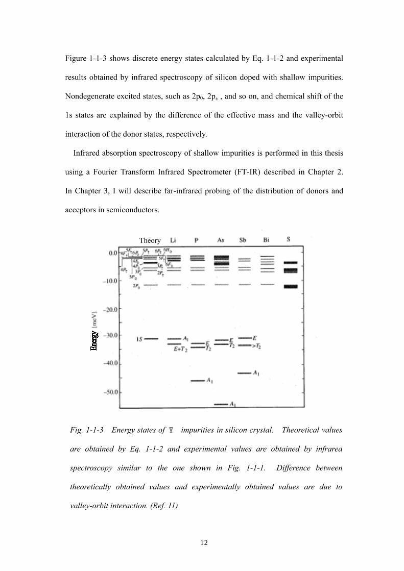
Figure 1-1-3 shows discrete energy states calculated by Eq. 1-1-2 and experimental
results obtained by infrared spectroscopy of silicon doped with shallow impurities.
Nondegenerate excited states, such as 2p0, 2p±, and so on, and chemical shift of the
1s states are explained by the difference of the effective mass and the valley-orbit
interaction of the donor states, respectively.
Infrared absorption spectroscopy of shallow impurities is performed in this thesis
using a Fourier Transform Infrared Spectrometer (FT-IR) described in Chapter 2.
In Chapter 3, I will describe far-infrared probing of the distribution of donors and
acceptors in semiconductors.
Theory
Fig. 1-1-3 Energy states of Ⅴ impurities in silicon crystal. Theoretical values
are obtained by Eq. 1-1-2 and experimental values are obtained by infrared
spectroscopy similar to the one shown in Fig. 1-1-1. Difference between
theoretically obtained values and experimentally obtained values are due to
valley-orbit interaction. (Ref. 11)

13
Broadening of the excited levels of shallow arsenic donors is measured and
compared with the prediction of competing theoretical models assuming different
distributions of ionized impurities. The electric field and its gradient due to ionized
donors and acceptors are treated as perturbations. The anisotropic wavefunctions
based on Kohn-Luttinger’s model 12 and Faulkner’s model 13 will be employed
successfully to explain the line broadening of the experimentally observed
absorption peaks. Based on the results, we show a clear evidence for the first time
that the distribution of ionized impurities in semiconductors can change between
correlated and random distributions. This finding is important both scientifically
and technologically. Understanding of ionized impurity distribution is of great
importance because it represents a complicated many-body problems where
Coulombic forces (electron-electron interactions) play important roles. Once
understood, engineers can perform a simple FTIR to characterize the donor and
acceptor concentrations in pure semiconductors.
14
1.2 Infrared spectroscopy of localized vibrational modes of impurities in
semiconductors – historical background and its relation to the work presented
in Chapter 4
As explained in the previous section, the addition of impurities to a semiconductor,
whether by design or accident, introduces energy levels into the band gap. In
addition to altering the electronic properties of semiconductors, impurities also affect
the vibrational properties. Atoms in a crystalline solid collectively oscillate about
their equilibrium positions, resulting in quantized vibrational modes known as
phonons. Einstein14 first treated the problem of phonons by assuming that the
atoms in a solid vibrate independently of one another. Debye15 improved the
Einstein model by treating a solid as an elastic continuum. In this thesis, the term
phonon is used to denote excitations that are extended in real space, involving the
motion of many atoms. Since phonons have a band of phonon frequencies, they are
also extended in frequency space.
As in the case of electrons in a perfect lattice, phonons in a perfect lattice have a
well-defined frequency ω and wave vector q. The ω vs q dispersion relation
can be experimentally determined via neutron scattering.16 When an impurity is
introduced, the translational symmetry is broken and one or more new vibrational
modes may appear. If a mass defect replaces a heavier host atom, for example, its
vibrational frequency will appear above the phonon frequency range. Unlike a
phonon, the vibrational mode of the defect is localized in real space and frequency
space, and is referred to as a local vibrational mode (LVM). Hydrogen, for
example, typically has LVM frequencies 5-10 times the maximum phonon frequency
and has narrow infrared (IR) absorption peaks.

15
The LVMs of impurities are affected by the symmetry of the surrounding
environment. The isotopic composition of the impurity-host system leads to
well-defined splitting and shifts of the vibrational frequencies. In Ge, GaAs, and
CdTe, the host-isotope disorder leads to complex LVM spectra that have been
modeled successfully. The host-isotope splitting provides a unique signature for
determining the site on which an impurity resides. The translational symmetry of a
perfect lattice is broken when a defect is introduced. As a simple example,
consider a harmonic linear chain, where one lattice mass is replaced by a smaller
mass. This model is used for long time within a small correction for many LVM
centers. The details of calculational model are mentioned in Chapter 4.
Fig. 1-2-1 Infrared absorption spectroscopy of interstitial oxygen in germanium
reported in Ref. 17.

16
Figure 1-2-1 shows infrared spectroscopy due to LVMs of interstitial oxygen in a
germanium crystal reported in Ref. 17. In Fig. 1-2-1, the frequencies of LVM
absorption lines depend on masses of oxygen and its two nearest neighboring
germanium atoms. For example, absorption lines labeled as 73.5Ge in Fig. 1-2-1
mean that interstitial oxygen atom is sandwiched by 73Ge and 74Ge atoms.
Symmetry of the potential energy at vibrating oxygen atoms makes a small splitting
of each absorption line. The difference of the intensity of an absorption line
corresponds to the composition of isotopes of a germanium crystal.
Oxygen is an omnipresent impurity in Czochralski-grown silicon, with serious
implications for the fabrication of integrated circuits. High concentrations (1018
cm-3) of oxygen are incorporated in Czochralski-grown crystals,18 as a result of the
dissolution of the SiO2 crucible at the growth temperature. Because an oxygen
atom is lighter than a silicon atom, it has local vibrational modes (LVM) in silicon
crystals. A review of the microscopic structure of oxygen in silicon is given by
Pajot.19 In as-grown silicon crystals, oxygen exists primarily as an interstitial
defect, denoted Oi. In this form, the oxygen binds with two silicon atoms and
resides between two silicon atoms aligned along the <111> direction. Under
uniaxial stress, Corbett, McDonald, and Watkins20 showed that stress along [111] or
[110] directions produced splitting of LVM peaks, whereas stress along the [100]
direction produced no splitting. These observations are consistent with complexes
aligned along the 〈111〉 axes. Ab initio calculations21 have shown that the Si-O
bond lengths to be 1.59 Å and the Si-O-Si bond angle to be 172°.
The most well studied oxygen LVM absorption peak is known as the 9 μm
line appearing at 1100 cm-1 at room temperature.22 The integrated intensity of this
particular absorption peak has become an industry standard for the determination of
17
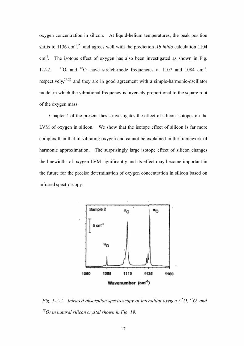
oxygen concentration in silicon. At liquid-helium temperatures, the peak position
shifts to 1136 cm-1,23 and agrees well with the prediction Ab initio calculation 1104
cm-1. The isotope effect of oxygen has also been investigated as shown in Fig.
1-2-2. 17Oi and 18Oi have stretch-mode frequencies at 1107 and 1084 cm-1,
respectively,24,25 and they are in good agreement with a simple-harmonic-oscillator
model in which the vibrational frequency is inversely proportional to the square root
of the oxygen mass.
Chapter 4 of the present thesis investigates the effect of silicon isotopes on the
LVM of oxygen in silicon. We show that the isotope effect of silicon is far more
complex than that of vibrating oxygen and cannot be explained in the framework of
harmonic approximation. The surprisingly large isotope effect of silicon changes
the linewidths of oxygen LVM significantly and its effect may become important in
the future for the precise determination of oxygen concentration in silicon based on
infrared spectroscopy.
Fig. 1-2-2 Infrared absorption spectroscopy of interstitial oxygen (16O, 17O, and
18O) in natural silicon crystal shown in Fig. 19.
18
References
1 C. P. Flynn, in Point Defects and Diffusion (Claredon, Oxford, 1972).
2 G. L. Pearson and J. Bardeen, Phys. Rev. 75, 865 (1949).
3 G. E. Stillman, D. M. Larsen, C. M. Wolfe, and R. C. Brandt, Solid State
Commum. 9, 2245 (1971).
4 N. F. Mott and R. F. Gurney, in Electric Processes in Ionic Crystals (Claredon,
Oxford, 1940).
5 D. Long, in Energy Bands in Semiconductors (Interscience, New York, 1968).
6 J. M. Whelan, in Properties of Some Covalent Semiconductors in Semiconductors,
(Reinhold, New York, 1960).
7 H. C. Torrey and C. A. Whitmer, in Crystal Rectifiers (McGraw-Hill, New York,
1948).
8 E. Burstein, G. Picus, B. Henvis, and R. Wallis, J. Phys. Chem. 57, 849 (1953).
9 E. H. Putley, Phys. Stat. Solidi. 6, 571 (1964).
10 C. Jaganaath, A. K. Ramdas, Phys. Rev. B 23 4426 (1981).
11 P. Y. Yu and M. Cardona, in Fundamentals of Semiconductors Physics and
Materials Properties Second Edition (Springer, Berlin Heidelberg, 1996) p.162.
12 W. Kohn and J. M. Luttinger, Phys. Rev. 98, 915 (1955).
13 R. A. Faulkner, Phys. Rev. 184, 713 (1969).
14 A. Einstein, Ann. Phys. (Leipzig) 22, 180 (1907); 22, 800 (1907).
15 P. Debye, Ann. Phys. (Leipzig) 39, 789 (1912).
16 B. N. Brockhouse and P. K. Iyergar, Phys. Rev. 111, 747 (1958).4c C. Kittel, in
Phonons, edited by R. W. H. Stevenson (Plenum, New York, 1966), Chap. 1.
17 A. J. Mayur, M. Dean Scicca, M. K. Udo, A. K. Ramdas, K. Itoh, J. Wolk, and E.
19
E. Haller, Phys. Rev. B 49, 16293 (1994).
18 C. Kittel, in Introduction to Solid State Physics First Edition (Wiley, New York,
1986), p. 83.
19 B. Pajot, Chapter V in Semiconductors and Semimetals 42 (Academic, New
York, 1994), p.191.
20 J. W. Corbett, R. S. McDonald, and G. D. Watkins, J. Phys. Chem.Solids 25, 873
(1964).
21 J. C. Mikkelson, Jr., Mater. Res. Soc. Symp. Proc. 59, 19 (1986).
22 R. Jones, A Umerski, and S. Oberg, Phys Rev. B 45, 11321 (1992).
23 R. J. Collins and H. Y. Fan, Phys Rev. 93, 674 (1954).
24 H. J. Hrostowski and R. H. Kaiser, Phys. Rev. 107, 966 (1957).
25 W. Kaiser, P. H. Keck, and C. F. Lange, Phys. Rev. 101, 1264 (1956).

20
Chapter 2: Infrared spectroscopy of semiconductors
Absorption spectra that will be presented in this thesis are recorded with a BOMEM
DA-8 Fourier Transform spectrometer. Basic elements of spectroscopy with the
BOMEM DA-8 are described in this chapter.
2.1 Michelson interferometer
The design of most interferometers used for infrared spectroscopy today is based
on that of two-beam interferometer originally designed by Michelson in 1891. The
Michelson interferometer is a device that can divide a beam of radiation into two
paths and then recombine the two beams after a path difference has been introduced.
A condition is thereby created under which interference between the beams can
occur. The intensity variations of the beam emerging from the interferometer can
be measured as a function of path difference by a detector. The simplest form of
the Michelson interferometer is shown Fig. 2-1-1.
Movable
Fixed mirror
Detector
Beamsplitter
Source
Mirror position
Fig. 2-1-1 Schematic representation of a Michelson interferometer.
Movable mirror
Fixed mirror
Detector
Beamsplitter
Source
Mirror position

21
It consists of two mutually perpendicular plane mirrors, one of which can move
along an axis that is perpendicular to its plane. The movable mirror is either moved
at a constant velocity or is held at equally spaced points for fixed short time periods
and rapidly stepped between these points. Between the fixed mirror and the
movable mirror is a beamsplitter, where a beam of radiation from an external source
can be partially reflected to the fixed mirror and partially transmitted to the movable
mirror. After the beams return to the beamsplitter, they interfere and are again
partially reflected and partially transmitted. Because of the effect of interference,
the intensity of each beam reaching to the detector and returning to the source
depends on the difference in path of the beams in the two arms of the interferometer.
The variation in the intensity of the beams passing to the detector and returning to
the source as a function of the path difference ultimately yields the spectral
information in a Fourier transform spectrometer. The source that returns to the
source is rarely of interest for spectrometry, and usually only the output beam
traveling in the direction perpendicular to that of the input beam is measured.
Nevertheless, it is important to remember that both of the output beams contain
equivalent information. The main reason for measuring only one of the output
beams is the difficulty of separating the output beam returning to the source from the
input beam. In some measurements, separate input beams can be passed into each
arm of the interferometer and the resultant signal measured using one or two
detectors.
The intensity of source power at the detector as a function of the position of the
movable mirror, which is named as interferogram, is transformed to the spectroscopy
as a function of the wave number with Fourier transformation as follows,

22
( ) ( ) ( )dxxxCI ⋅= ∫∞
∞−ω
πω cos1 , (2-1-1)
where C(x) is the intensity of the interferogram when the movable mirror position is
at x. It is impossible to move the movable mirror from infinity to minus infinity,
that is, we can’t use Eq. (2-1-1) directly in actual measurements. If we integrate the
interferogram from –L (the limiting position of the movable mirror) to +L, and there
are fringes in a spectrum near the peaks, then the line shape function will have the
form of (sinx)/x since the spectrum is obtained from the Fourier transition of the step
function. In order to avoid making fringes in the spectrum, we must adjust the
interferogram gradually to zero with Apodization functions as the position of the
movable mirror is going to –L or L. The advantage of using Apodization functions
is the reduction of the fringes near the peaks in the spectrum.
Fig. 2-1-2 Relation between the interferogram and spectroscopy as a
function of a wavenumber. The interferogram is obtained from the intensities
as a function of the position of the movable mirror summed for each wave
number. The spectroscopy is obtained after the interferogram is transformed
with Fourier transformation, Eq. (2-1-1).
Position of the movable mirror
Fourier
Wavenumber
Intensity
Transform
23
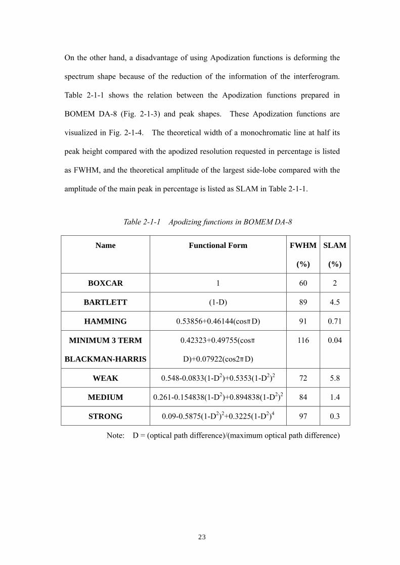
On the other hand, a disadvantage of using Apodization functions is deforming the
spectrum shape because of the reduction of the information of the interferogram.
Table 2-1-1 shows the relation between the Apodization functions prepared in
BOMEM DA-8 (Fig. 2-1-3) and peak shapes. These Apodization functions are
visualized in Fig. 2-1-4. The theoretical width of a monochromatic line at half its
peak height compared with the apodized resolution requested in percentage is listed
as FWHM, and the theoretical amplitude of the largest side-lobe compared with the
amplitude of the main peak in percentage is listed as SLAM in Table 2-1-1.
Name Functional Form FWHM
(%)
SLAM
(%)
BOXCAR 1 60 2
BARTLETT (1-D) 89 4.5
HAMMING 0.53856+0.46144(cosπD) 91 0.71
MINIMUM 3 TERM
BLACKMAN-HARRIS
0.42323+0.49755(cosπ
D)+0.07922(cos2πD)
116 0.04
WEAK 0.548-0.0833(1-D2)+0.5353(1-D2)2 72 5.8
MEDIUM 0.261-0.154838(1-D2)+0.894838(1-D2)2 84 1.4
STRONG 0.09-0.5875(1-D2)2+0.3225(1-D2)4 97 0.3
Note: D = (optical path difference)/(maximum optical path difference)
Table 2-1-1 Apodizing functions in BOMEM DA-8
24
0
0.2
0.4
0.6
0.8
1
-1 -0.5 0 0.5 1
Boxcar
Bratlet
HammingBlackman-HarrisWeak
Medium
Strong
可動鏡の位置/可動鏡の最大移動距離D (optical path difference / maximum optical path
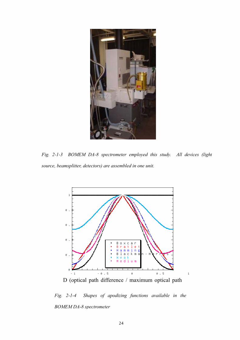
Fig. 2-1-4 Shapes of apodizing functions available in the
BOMEM DA-8 spectrometer
Fig. 2-1-3 BOMEM DA-8 spectrometer employed this study. All devices (light
source, beamsplitter, detectors) are assembled in one unit.

25
Therefore, it is important for us to consider the effect of the broadening due to
Apodization functions. Apodization functions listed in Table 2-1-1 can be divided
into two classes:
1: those appropriate for very sharp peaks (width less than 0.1 cm-1) and
2: those appropriate for the width of the order ~1 cm-1.
In case the linewidth is very small (width less than 0.1 cm-1), we can see the
effect of Apodization function on linewidths clearly. Figure 2-1-5 shows
absorption spectra of water molecules (moisture in the air) vibration apodized by the
functions listed in Table 2-1-1.
1610 1620 1630 1640 1650
BoxcarBartlettHammingBlackmanWeakMediumStrong
Abs
orba
nce
[a.u
.]
Wavenumber [cm-1]Fig. 2-1-5 Absorption spectra due to H2O vibrations measured at room
temperature apodized by a variety of functions. These sharp features represent
lines of different vibration modes.

26
We focus of the linewidth measured at 1616.8 cm-1 in Fig. 2-1-5 in order to compare
the effect of Apodization functions. In Fig. 2-1-6, dotted points and solid lines
represent experimentally obtained data and Lorentzian fitting to them, respectively.
We obtained the linewidths (full width at half maximum) of each line by fits using
the Lorentzian function. The lines apodized by different functions have different
linewidths. This difference approximately agrees with the list in Table 2-1-1.
Therefore, the selection of Apodization function is important when we discuss the
linewidth of very narrow absorption lines.
BoxcarBartlettHammingBlackmanWeakMediumStrong
Abs
orba
nce
[a.u
.]
Wavenumber [cm-1]1616.0 1616.5 1617.0 1617.5
Fig. 2-1-6 Absorption lines of moisture vibrations measured at
1616.8cm-1 for different Apodization functions. The absorption lines
apodized by different functions have different widths.

27
Apodization function Linewidth of moisture at 1616.8 cm-1
BOXCAR 0.084
BARTLETT 0.133
HAMMING 0.190
MINIMUM 3 TERM BRACKMAN-HARRIS 0.140
WEAK 0.099
MEDIUM 0.109
STRONG 0.120
Next, we considered the effect of Apodization functions on absorption
linewidths when the lines are not so narrow (the width of more than 0.1 cm-1).
Figure 2-1-7 shows far infrared spectra of acceptor excitation bound to boron
impurities in silicon at 4 K. We find several peaks in this figure and they are
assigned to the transitions from the ground state to the discrete excited states of
boron acceptors. As an example, the widths of the peaks at 278 cm-1 are compared
in Fig. 2-1-8. Dotted points mean experimental results and the solid lines are
Lorentzian fitting to them. We find that the peak apodized by Bartlett function is
significanly broadened. However, other peaks are not so broadened. It is because
interferogram at the positions near the center is largely reduced by the Bartlett
function, while those by other Apodization functions are not reduced so much (see
Fig.2-1-4). The linewidths obtained by Lorentzian fitting are listed in Table 2-1-3.
Table 2-1-2 Linewidths (Full width at half maximum) of H2O molecule vibration
measured at 1616.8 cm-1 for each Apodization function.

28
240 260 280 300 320
BoxcarBartletHammingBlackmanWeakMediumStrong
Abs
orba
nce
[a.u
.]
Wavenumber [cm-1]
Si:B ([B]=2.63x10¹⁵) at T=4K
Fig. 2-1-7 Infrared spectra of Si:B measured at 4 K apodized by the seven
functions listed in Table 2-1-1.
275 276 277 278 279 280 281 282
BoxcarBartletHammingBlackmanWeakMediumStrong
Abs
orba
nce
[a.c
.]
Wavenuber [cm-1]
Si:B ([B]=2.63x10¹⁵) at T=4K
Fig. 2-1-6 Infrared spectra of Si:B measured at 4 K apodized by the seven
functions listed in Table 2-1-1. Dotted points are experimental results and
solid lines are Lorentzian fittings.

29
Apodization function Linewidth of boron line at 278 cm-1
BOXCAR 0.97
BARTLETT 1.23
HAMMING 1.00
MINIMUM 3 TERM BRACKMAN-HARRIS 0.99
WEAK 1.01
MEDIUM 1.00
STRONG 1.0
Table 2-1-3 shows clearly that the choice of Apodization functions (except for
Bartlett) does not lead to significant change in the linewidths when the width is
larger than 1 cm-1. Because widths of all the peaks we study in this work are of the
order of 1 cm-1, the effect of apodization is negligibly small.
Table 2-1-3 Linewidths (Full width at half maximum) of boron peaks at 278 cm-1
for each Apodization function.

30
2.2 Phase
In an ideal interferometer, the optical paths of the two perpendicular routs are
perfectly aligned and all waves interfere constructively at so called the zero path
difference (ZPD), where the lengths of the two routs are equal. In such an
interferometer, the cosine Fourier Transform always yields the correct spectrum.
In practice, however, both dispersion and sample shifts occur with respect to the
ZPD position. These effects are usually corrected for by a so-called phase
correction procedure performed for every measured interferogram. The phase is
calculated from the expression:
( ) ( ) ( )σσσ ri MMarctan−=Θ , (2-2-1)
where Mi( σ) and Mr( σ) are the imaginary and real components, respectively, of the
Fourier Transform of the interferogram at a particular wavenumber. Since
interferometric spectrometers may be employed for the spectral measurement of a
wide variety of transmission, the character of the interferograms produced by the
samples or source under investigation may be equally varied. As a consequence,
the phase information obtained by the complex transformation may not always be
fully representative of the phase response of the interferometer, i.e., phase errors may
become apparent in the recovered spectrum.
Due to the excellent alignment stability of BOMEM DA-8 spectrometer
achieved by the use of dynamic alignment, the dispersion and sample shift (phase
characteristic) of the interferometer are time invariant. In this situation, a
pre-calibration of the phase character of each interferometer can be carried out by
31
executing the functional step ‘Phase’ using the most suitable source and detector for
this task. The phase calibration curve is stored in the associated data system for
future use in interferogram symmetry.
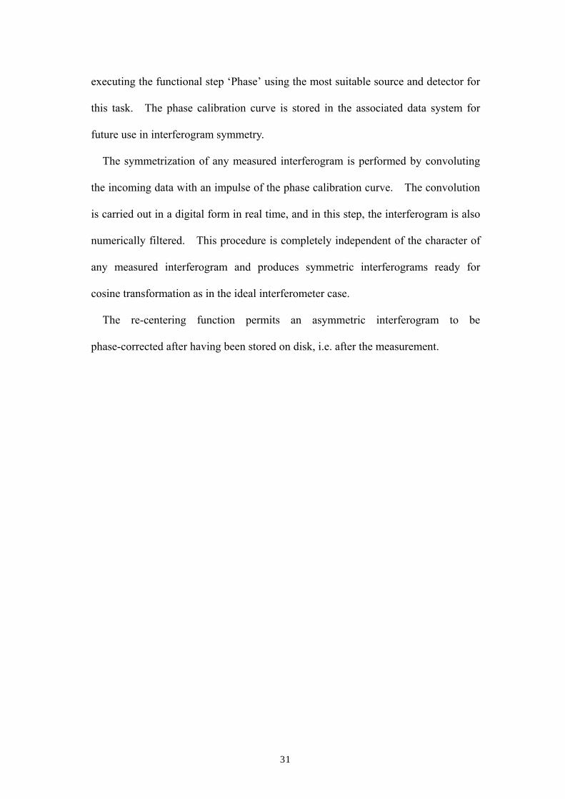
The symmetrization of any measured interferogram is performed by convoluting
the incoming data with an impulse of the phase calibration curve. The convolution
is carried out in a digital form in real time, and in this step, the interferogram is also
numerically filtered. This procedure is completely independent of the character of
any measured interferogram and produces symmetric interferograms ready for
cosine transformation as in the ideal interferometer case.
The re-centering function permits an asymmetric interferogram to be
phase-corrected after having been stored on disk, i.e. after the measurement.

32
2.3 Resolution
In an interferometric spectrometer, the resolution is a function of the distance
traveled by the moving mirror, the apodizing function selected, and the criterion used
to judge this parameter. For an optimally aligned instrument observing a
monochromatic source those radiation is perfectly parallel to the optical axis of the
interferometer, it may be shown that for an unapodized interferogram the line shape
function will have the form (sin x)/x, and that for an infinitely large signal-to-noise
ratio, the full width of the resulting spectral line at half of its line height, FWHM,
will be:
LFWHM
22067.1
= (2-3-1)
where L is the maximum optical path difference.
This theoretical value is the best that can be achieved but in practice, this value
may be degraded by several factors. An unapodized interferogram produces large
spurious side lobes associated with individual spectral features; the usual practice is
to apodize the interferogram in order to reduce the contribution due to these features.
Each of Apodizing functions reduces the side lobes in a slightly different manner and
it is up to us to choose whichever is preferable in a given application. There is,
however, one major effect of reducing the intensity of the side lobes: there is a
corresponding increase in the width of the spectral features. For the most severe
Apodization offered, the FWHM value is increased to approximately 2.0/2L. This
worst case is taken for the apodized resolution (RE) specified; i. e.

33
LRE 1
= . (2-3-2)
For most of the Apodizing functions available, the apodized resolution value is a
conservative estimate of the resolution that should be achieved when operating the
spectrometer. One may sometimes want to calculate more points in the spectrum
than existed in the original interferogram. This has the effect of producing a
smoother spectrum, but does not change the resolution in any way. The
interpolation is usually performed in passing from the interferogram to the spectral
domain by the procedures of zero-filling or over-sampling, a transmission spectrum
of n points is calculated from a discrete finite interferogram having m real data
points, by a matrix product. In zero-filling a series of m zero elements are filled to
satisfy the condition n=m-2k where k is an integer. In over-sampling the Fourier
transformation is performed using a rectangular n×m matrix, yielding an n-point
spectrum from an m-point interferogram having no zero elements. The two
procedures yield identical results and the choice between them depends on how the
FT is carried out.
In order to obtain a satisfactory detector signal, it is sometimes desirable to
employ a lager optical aperture at the focal point of the collimation mirror. This
has two effects: to increase the intensity of the interferometer beam, and to increase
its divergence. The divergence of the collimated beam is related to the precision of
the optical path difference obtained; a less precise optical pass difference results in a
smearing of interferogram modulation, which places a limit on attainable spectral
resolution. It is therefore necessary, for high-resolution measurements, to restrict
the effective field of view (aperture size) of the instrument. The maximum aperture

34
diameter is related to the apodized resolution RE and the maximum phase frequency
SX by:
21
2_
××=
SXREFLdiaAperture (2-3-3)
where FL is the focal length of the input collimating mirror. Also, when
performing emission experiments particularly, selecting an inappropriate aperture
size may results in frequency shift problems. For experiments where the aperture
opening is not fully covered with radiation, it is required to reduce the size of the
aperture until the aperture size approximately fits the throughput of our experiment.
This is particularly important for experiments where no physical aperture is used; in
this case, set the software aperture size as if an aperture was used.
The rapid scanning mode of operation is used almost exclusively in present day
commercial interferometric spectrometers. In this model the frequency of an
infrared signal as represented in the interferogram is a simple function of the infrared
wavenumber and the travel speed of the moving mirror. The digital representation
of such an interferogram signal must be obtained at a sample rate that is at least
twice the maximum frequency generated in order that all information must be
retained. Note that this maximum frequency might not be due to the signal of
interest but might be caused by a spurious signal or by noise. By strongly
suppressing all frequencies outside the range of interest, the number of interferogram
samples may be kept to a minimum with the attendant shortening of transformation
times and easing of memory requirements.
Strong suppression of frequencies outside a range of interest by means of
35
electrical filtering becomes increasingly difficult as the ratio of the mean frequency
to the bandwidth of interest increases. This difficulty arises in designing sharp
cut-on and cut-off electrical filters having low distortion, and which can be
programmed over a wide range of frequencies. Furthermore, since electrical
frequencies relate directly to spectral frequencies via the velocity of the
interferometer mirror, a high degree of velocity stability is required. This later
approach suggests the need for frequent sampling of the signal. In order to
facilitate frequent sampling of an interferogram with minimal electrical filtering,
while at the same time minimizing the volume of stored data, BOMEM uses a Vector
Processor, that it developed, programmed to numerically filter incoming data in real
time. Only the result after numerical filtering is stored in memory, either as a single
scan or coadded to previous scans for subsequent Fourier transformation also
performed by the Vector Processor. The Vector Processor is sufficiently rapid to
filter data at a rate of up to 400,000 samples per second with flexible data
compression factors ranging from 1 to 127.
The filter process consists of convolving the incoming interferogram data with a
finite impulse response function that is the Fourier Transform of the desired spectral
filter response. Using the properties of convolution, this is equivalent to
multiplying the Fourier transform of the interferogram, i.e. the spectrum, with the
desired spectral filter response. The filter response is near unity over the spectral
band of interest and drops off to provide very high rejection just outside the band.
The frequencies of the numerical filter response are proportional to the sample
frequency. When the samples are synchronized with specific mirror positions, as is
the case for laser-fringe sampling, the numerical filter response becomes locked to
spectral frequencies and is independent of mirror velocities or electrical frequencies.
36
Since the numerical filter response is a well-defined function in the spectral
frequency domain, it can be used to suppress out-of-band spectral features.
As an example of this technique, an InSb detector may be used to detect
radiation in a band from 1820 cm-1 to 4000 cm-1 as defined by a long pass filter and
the detector cut-off. Interferograms for this spectral region are normally sampled
by a He-Ne laser at 15798 samples per cm of optical path difference, resulting in
4×10⁶ samples for the full-mirror displacement of a model DA-8. If, however, it is
of interest to study only a part of this bandwidth, for example the υ1 and 2υ2 bands of
carbonyl fluoride that are located between 1890 or above 1985 cm-1, the number of
samples in the interferogram may be greatly reduced. This reduction factor is
calculated as follows: Consider a signal that has a bandwidth that falls within a
lower and upper frequency limit, σ(min) andσ(max), such that:
( ) ( )δσσ 1min −= n (2-3-4)
( ) δσσ n=max (2-3-5)
where ( ) ( )minmax σσδσ −= .
Then a sampling frequency of δσ2 may be used to unambiguously represent all
information in the signal, and under this scheme, the signal will occur in the n-th
alias. In the example of the υ1 and 2υ2 bands of carbonyl fluoride (COF2) as
mentioned above, if a sample rate of 336.13 samples per cm of optical path
difference is selected, then n=12, σ (min)=1849 cm-1, andσ(max)=2017 cm-1. It can
be seen therefore that the two bands of carbonyl fluoride occur in the twelfth alias
when sampled at 1/47 of the laser fringe frequency and no information is lost by
applying numerical filtering with the above criteria. The maximum number of

37
samples to be stored is now reduced by a factor of 47, i.e. 84,000 instead of the
4×10⁶ samples obtained for full resolution with a DA-8 system. As a rule, after
numerical filtering, a new sample frequency can be chosen that is an integer fraction
of the laser fringe frequency and which is equal to or greater than twice the
bandwidth. The roll-off from unity to 10-6 gain is proportional to the bandwidth
and may vary from 3% to 10% depending on a number of operating parameters.
The software accompanying the DA-8 system is designed so that for any given lower
and upper frequency, a filter function is automatically generated along with a best
data compression factor and operating alias suggested by the Phase function. By
incorporating the inverse of the phase distortion of the interferometer into the
response function, interferograms stored after numerical filtering, therefore, need
only cosine Fourier transformation in order to yield the correct spectrum.
38
2.4 Spectral range
The net spectral range of the spectrometer is determined by the combination of
resources employed. The source, optical filter, beamsplitter, and detector each has
a limited spectral range. The sources radiate over spectral bands determined by the
materials and conditions employed (glowing solid, incandescent gas, pressure,
temperature, and so on). The spectral ranges of the beamspliters and windows are a
function of substrate and coating materials. The radiation detectors exploit a
variety of physical processes for sensitivity to spectral bands from far infrared to
ultraviolet. The spectral range is also determined by the data sampling. The
maximum wavenumber value is used to define the number of samples per laser
fringe obtained from the analog interferogram signal by the analog-to-digital
converter (ADC). Since the He-Ne laser is used for sampling the interferogram
signal and the detector exit emits a monochromatic beam of radiation at 15798 cm-1,
the maximum wavenumber that may be accommodated without aliasing is:
n×××2
15798,22
15798,12
15798L (2-4-1)
for 1, 2, …, n samples of the interferometer signal per laser fringe. In the PCDA
software that accompanies the DA-8, there is a choice of 1, 2, 4, or 8 samples per
laser fringe, permitting spectral bandwidths of from 0 cm-1 to 7899 cm-1 (1.266µm),
15798 cm-1 (0.633µm), 31596 cm-1 (0.316µm), and 63192 cm-1 (0.158µm),
respectively, without aliasing.
39
2.5 Detector response and scan speed
The following three detector properties directly affect the quality of
measurements made by the spectrometer:
1. spectral response;
2. response time;
3. frequency response.
The response time is the delay between an impulse of radiation and the peak
electrical output from the detector/preamplifier combination. The time delay can
differ by up to 5 orders of magnitude for different classes of detector, as summarized
in Table 2-5-1. The delay introduced minimizes the effect of speed variations on
the interferogram signal, and also, when using the technique of stored phase
characterization, permits application of one set of phase coefficients over a range of
scanning speeds. The response time is usually related to the 3 dB cutoff frequency
of the detector/preamplifier pair. The selection of the speed in a particular
experiment is based on several factors, however. The most important relates to the
frequency response of the detector. Each detector is supplied with a response curve
that shows the relative detector response as a function of the chopping frequency of
the signal on the detector element. A suitably matched preamplifier should not
alter this response curve significantly. For a rapid scanning interferometer the
output signal fringe frequency (FR, measured in Hz) is a function of the
wavenumber of interest (NU in cm-1) and the mechanical speed of the moving mirror
(SP in cm/s) as follows:
SPNUFR ⋅⋅= 2 (2-5-1)

40
Thus, for a specified spectral bandwidth, a speed may be chosen that is optimal with
respect to the response curve of the detector/preamplifier combination. For
example, the frequency response curve of a typical MCT (Hg-Cd-Te) detector shows
that this detector should be operated so that the infrared fringe frequencies lie within
400 Hz to 1 MHz. If the user decides to operate the system so that the spectral
bandwidth from 450 cm-1 to 5000 cm-1 is covered, then a speed of 0.5 cm/s would
produce a modulated output signal containing frequencies between 450 Hz (450
cm-1) and 5 kHz (5000 cm-1). Thus, as long as the preamplifier is matched to give
a uniform response at these frequencies, the interferometer should be operated with a
rapid moving mirror velocity for this particular detector/bandwidth combination.
Table 2-5-1 presents the 16 mirror scanning speeds available and also lists the
sampling frequency (i.e. conversion frequency of the ADC) for operation at the 4
samples per laser fringe values possible. Notes:
(a) The laser fringe frequency is the effective frequency of the He-Ne
laser fringes on the laser detectors.
(b) The sampling frequency is the rate at which the infrared signal is
sampled and is the laser fringe frequency multiplied by the number of
samples taken every laser fringe.
(c) Speeds lower than 0.05 may cause problems with stability, especially
as the number of samples per laser fringe is increased.
It should be noted that there are two other major limiting factors with respect to
the speed of the moving mirror: these relate to the conversion speed of the
analog-to-digital converter (ADC) and the speed of operation of the Vector Processor
system. As may be seen from Table 2-5-1, the conversion speed of the 16-bit ADC

41
limits the scanning speed to 1.5 cm/s, or less, at 1 sample-laser fringe if the full
resolution of the ADC is required, and with the other indicated values at faster
sampling rates.
Speed
(cm/s)
mechanical
Laser fringe
frequency
(kHz)
Time delay
1 2 4 8
0.01 0.316 0.316 0.632 1.26 2.53
0.02 0.632 0.632 1.26 2.53 5.06
0.03 0.948 0.948 1.90 3.79 7.58
0.05 1.58 1.58 3.16 6.32 12.6
0.07 2.21 2.21 4.42 8.84 17.7
0.10 3.16 3.16 6.32 12.6 25.3
0.15 4.74 4.74 9.48 19.0 37.9
0.2 6.32 6.32 12.6 25.3 50.6
0.3 9.48 9.48 19.0 37.9 75.8
0.5 15.8 15.8 31.6 63.2 1226.0
0.7 22.1 22.1 44.2 88.4 177.
1.0 31.6 31.6 63.2 126.0 253.
1.5 47.4 47.4 94.8 190. 379.
2.0 63.2 63.2 126.0 253. 506.
3.0 94.8 94.8 190. 379. 758.
4.6 145. 145. 290. 580. 1160.
Table 2-5-1 Scanning speed parameters and corresponding time delays
42
The major limitation in speed with respect to the Vector Processor is the rate at
which the coadding may be performed in the memory. This is a function of the data
reduction factor and the laser fringe frequency. The coadding rate is limited to 200
kHz and will be the speed limiting factor if using a fast ADC of 200kHz or above.
Instabilities in the dynamic alignment system may also be found to occur when the
moving mirror is driven at very low speeds.

43
2.6 Combination of elements in BOMEM DA-8 FT spectrometer
There are total of three sources, seven beamsplitters, and six detectors, as
summarized in Table 2-6-1, for the system we employed in the present thesis. The
combination of these elements depends on the spectrum region needed for our
investigation.
Source Beamsplitter Detector
Mercury 5~200 FIR 125u 3~25 Bolometer(1) 3~100
Globar 200~10000 FIR 50u 10~50 Bolometer(2) 10~700
Quartz 2000~25000 FIR 25u 15~100 DTGS/FIR 10~700
FIR 6u 75~450 MCT/KRs5 400~5000
FIR WIDE 125~850 InSb/AMc 3200~14000
KBr 450~4000 Si 8500~50000
Visible 4000~25000
(in unit of cm-1)
For example, a combination of the Globar source, KBr beamsplitter, and MCT/KRs5
detector span a spectrum range from 450 to 4000 cm-1, since the highest
wavenumber of minimum valid one among the three devices (Globar is 200 cm-1,
KBr is 450 cm-1, and MCT/KRs5 is 400 cm-1) is 450 cm-1 and the lowest
Table 2-6-1 Elements of BOMEM DA-8

44
wavenumber of maximum valid one among the three devices (Globar is 10000 cm-1,
KBr is 4000 cm-1, and MCT/KRs5 is 5000 cm-1) is 4000 cm-1. Figure 2-6-1 shows
two raw spectra for the combination of Globar, KBr, and MCT/KRs5 with and
without a cryostat we used. The vertical axis represents the intensity of
transmission, and horizontal axis represents frequency. Absorption measured at
1200 and 2800 cm-1 is due to the beamsplitter. Absorption lines measured from
1500 to 2000 cm-1 and from 3500 to 4000 cm-1 are due to vibrations of H2O
molecules existing in the sample room. We used cryostat with four ZnSe windows
which reduces the light transmission intensity further. Spectra shown in Chapter 4
were recorded in this setting (Globar, KBr, MCT/KRs5, and the cryostat with four
ZnSe windows).
1000 2000 3000 4000 5000
Without OPTISTATWith OPTISTAT
Inte
nsity
[a.u
.]
Wavenumber [cm-1]
Fig. 2-6-1 Raw spectra with and without a cryostat. Source is Globar,
beamsplitter is KBr, and detector is MCT. We used these spectra as
background of our measurement.
45
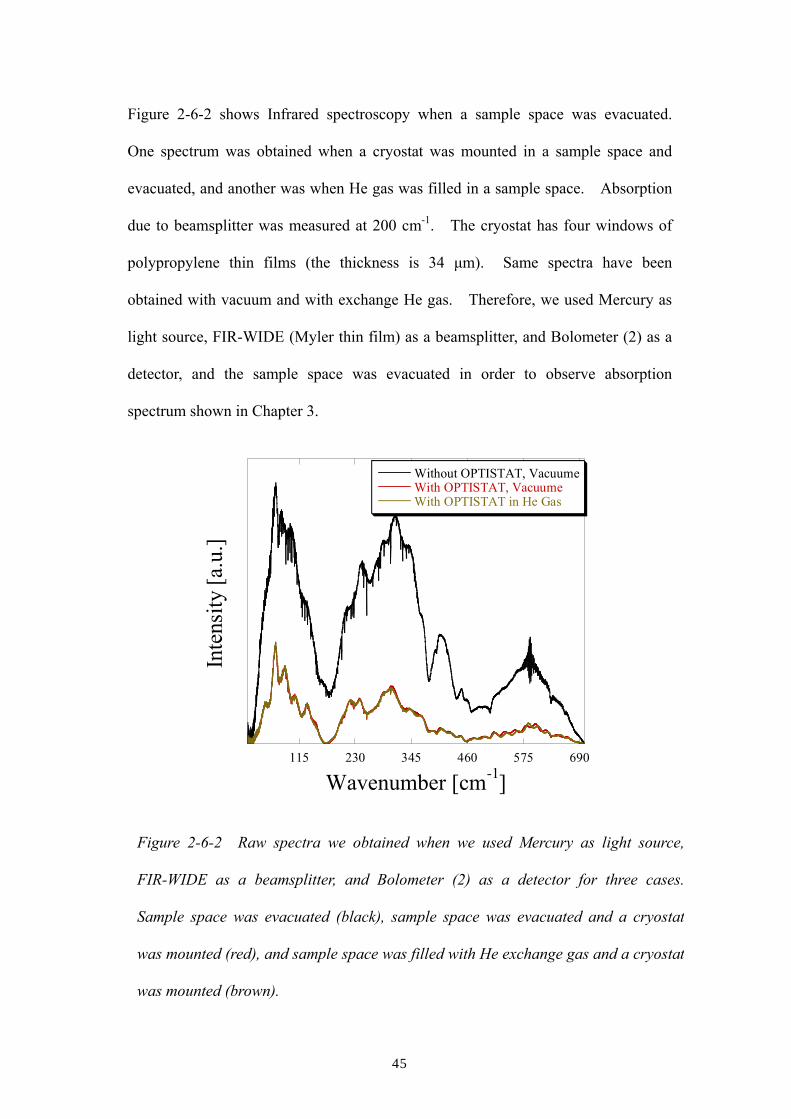
Figure 2-6-2 shows Infrared spectroscopy when a sample space was evacuated.
One spectrum was obtained when a cryostat was mounted in a sample space and
evacuated, and another was when He gas was filled in a sample space. Absorption
due to beamsplitter was measured at 200 cm-1. The cryostat has four windows of
polypropylene thin films (the thickness is 34 µm). Same spectra have been
obtained with vacuum and with exchange He gas. Therefore, we used Mercury as
light source, FIR-WIDE (Myler thin film) as a beamsplitter, and Bolometer (2) as a
detector, and the sample space was evacuated in order to observe absorption
spectrum shown in Chapter 3.
115 230 345 460 575 690
Without OPTISTAT, VacuumeWith OPTISTAT, VacuumeWith OPTISTAT in He Gas
Inte
nsity
[a.u
.]
Wavenumber [cm-1]
Figure 2-6-2 Raw spectra we obtained when we used Mercury as light source,
FIR-WIDE as a beamsplitter, and Bolometer (2) as a detector for three cases.
Sample space was evacuated (black), sample space was evacuated and a cryostat
was mounted (red), and sample space was filled with He exchange gas and a cryostat
was mounted (brown).
46
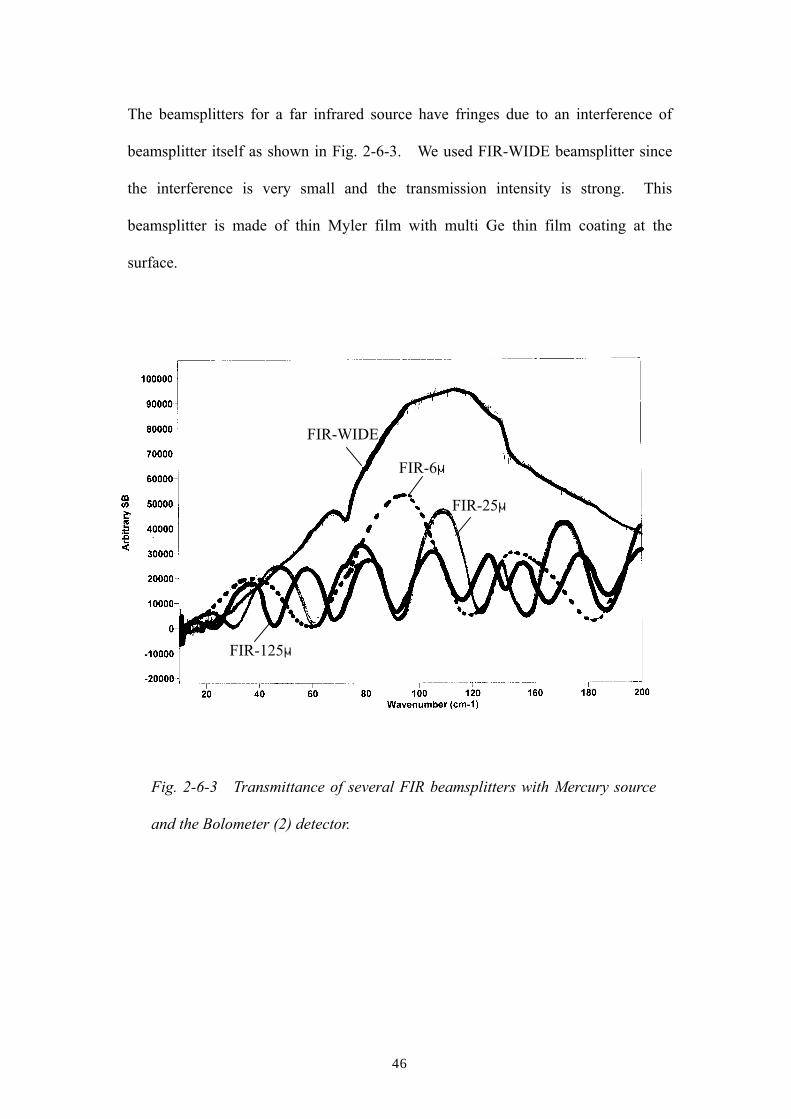
The beamsplitters for a far infrared source have fringes due to an interference of
beamsplitter itself as shown in Fig. 2-6-3. We used FIR-WIDE beamsplitter since
the interference is very small and the transmission intensity is strong. This
beamsplitter is made of thin Myler film with multi Ge thin film coating at the
surface.
FIR-WIDE
FIR-6μ
FIR-25μ
FIR-125μ
Fig. 2-6-3 Transmittance of several FIR beamsplitters with Mercury source
and the Bolometer (2) detector.

47
2.7 Calculation of the absorption coefficient
Absorption coefficient α is obtained by the measurements of transmittance
spectroscopies with and without inserting a sample. The spectrum of incident light
to the sample (Iin) is obtained by the measurement without a sample, while the
spectrum through a sample (Iout) is obtained with inserting a sample as shown in Fig.
2-7-1. The formula of absorption coefficient is given generally by the following;1
=
IoutIin
Lln1
α , (2-7-1)
where L is the thickness of a measured sample. However, multi-reflection within a
sample due to the high refractive index of a sample must be considered for the case
of semiconductor samples.
Fig. 2-7-1 An illustration of incident and transmitted lights
Sample
Thickness L

48
Equation 2-7-1 is used when we obtain absorption coefficient of low refractive index
materials, for example, gas and organic compounds. However, when we obtain
absorption coefficient of high refractive index materials, we must consider losses of
reflection at a surface of a sample and multiple reflections inside a sample. The
absorption coefficient for high refractive index materials is obtained by2
( ) ( )
−−+−=
221224
2
1412ln1
RTRRTR
Lα , (2-7-2)
where
( ) ( )( )LR
LRIIT
IN
out
αα
2exp1exp1
2
2
−−−−
== (2-7-3)
and
( )( )2
2
11
nnR
+−
= . (2-7-4)
For example, the reflection ratio of germanium is obtained by using a refractive
index n of 3.98 in this thesis.
The Lorentzian function Γ is used to fit absorption peaks arising from
bound-electronic transition and the local vibrational modes of impurities. The
function is given by :
( ) ( )220 2
2βωω
βχΓ
+−= , (2-7-5)
49
where χ is the intensity of the peak, ω is the frequency, and β is the full width at half
maximum (FWHM) of the peak. The linewidth in this thesis is obtained by fitting
with a Lorentzian function defined by Eq. (2-7-5).

50
2.8 IR absorption measurement procedures
All of the infrared absorption spectra appearing in this thesis have been
recorded with BOMEM DA-8 Fourier transform spectrometer as described in detail
in the previous sections. I will describe the practical aspect of the measurements in
this last section of Chapter 2.
Samples were wedged in order to avoid the constructive interference of
reflected waves inside samples. If the sample has parallel surfaces, the
wavelengths corresponding to the fraction of integer multiples constructively
interfere as illustrated in Fig. 2-8-1. Therefore, we make unparallel samples
which have less than 1°wedging by lapping with SiC slurry as depictured in Fig.
2-8-2.
Sample
Wavenumber
Fig. 2-8-1 Illustration of interference due to uniform sample thickness (left
picture) and absorption spectrum with interference (right picture). The small
fringes in the spectrum are due to interference.

51
Removing of the alias patterns in the interferogram is an additional effective
way to erasing interfering fringes in the spectra. This procedure normally known as
zapping is shown in Figure 2-8-3. Fig. 2-8-3 (b) shows interferogram of the
Fourier transformed infrared spectrum in Fig. 2-8-3 (a). A position of the
maximum intensity of interferogram is at the zero-path difference (the distance from
the beamsplitter to the fixed mirror is equal to that from the beamsplitter to the
movable mirror) in Fig. 2-8-3 (b). The ghost (alias) peak due to the constructive
interference of samples is seen in right part of Fig. 2-8-3 (b). Figure 2-8-3 (d) is
obtained by zapping the ghost peak in Fig. 2-8-3 (b). Figure 2-8-3 (c) demonstrates
the infrared spectrum obtain by Fourier transformation of the zapped interferogram
shown in Figure 2-8-3 (d), which show no interfering fringes. The linewidth of the
spectrum does not change before and after zapping. Therefore, we employ in this
study a combination of the sample wedging and interference zapping in order to
reduce fringes in the spectra.
Fig. 2-8-2 Illustration of a lapping equipment that allows for precise
wedging of samples.
Sample
SiC slurry
Glass plate

52
During the measurements, the signal-to-noise ratio was improved by coadding
100 to 720 spectra. A composite silicon bolometer operating at T = 4.2 K was used
as a detector. The samples were cooled in the OXFORD OPTISTAT cryostat and the
sample temperature was monitored with a calibrated thermometer installed at the
sample mount. A black-polyethylene film (34 µm thick) was used in front of samples
to eliminate above band-gap radiation.
Fig. 2-8-3 (a) A spectrum obtained by Fourier transformation of the
interferogram shown in (b). A zapped interferogram shown in (d) leads to a
fringe-less spectrum shown in (d). This series of spectra obtained by Ge:As of no
wedging. A clear As absorption line is seen at about 100 cm-1.
(a) (b)
(c) (d)
53
References
1 P. Y. Yu and M. Cardona, in Fundamentals of Semiconductors Physics and
Materials Properties Second Edition (Springer, Berlin Heidelberg, 1996) p.236.
2 P. R. Griffiths and J. A. de Hanseth, in Fourier Transform Infrared Spectrometry
(John Wiley, New York, 1986) p.308.

54
Chapter Ⅲ: Observation of the Random-to-Correlated Transition
of the Ionized Impurity Distribution in Compensated
Semiconductors
3.1 Introduction
Many-body Coulombic interactions between randomly distributed positive and
negative charges play important roles in a wide variety of physical systems. Such
interactions become important especially when the charges are mobile and
redistribute themselves in order to minimize the total Coulombic energy of the
system. Itoh, et. al. have shown recently that compensated semiconductors, e.g.,
germanium doped simultaneously by hydrogenic donors and acceptors, serve as
ideal systems for the investigation of many-body Coulombic interactions between
mobile ions.1 Let us define a problem of our interest as the following. Consider a
n-type semiconductor with the concentration of hydrogenic donors (ND) being twice
of that of hydrogenic acceptors (NA); ND= 2NA. As Fig.3-1-1 shows, at sufficiently
low temperatures one half of ND is positively charged (21 ND=ND
+) because their
bound-electrons are taken away by acceptors. These become negatively charged after
accepting electrons (NA=NA-). The remaining half of ND binds electrons so that
their charge state is neutral (21 ND=ND
o). This system is interesting because the
ionized donors (D+) can modify their distribution with respect to the fixed position of
ionized acceptors (A-) via the transfer of electrons between neutral (D0) and ionized
55
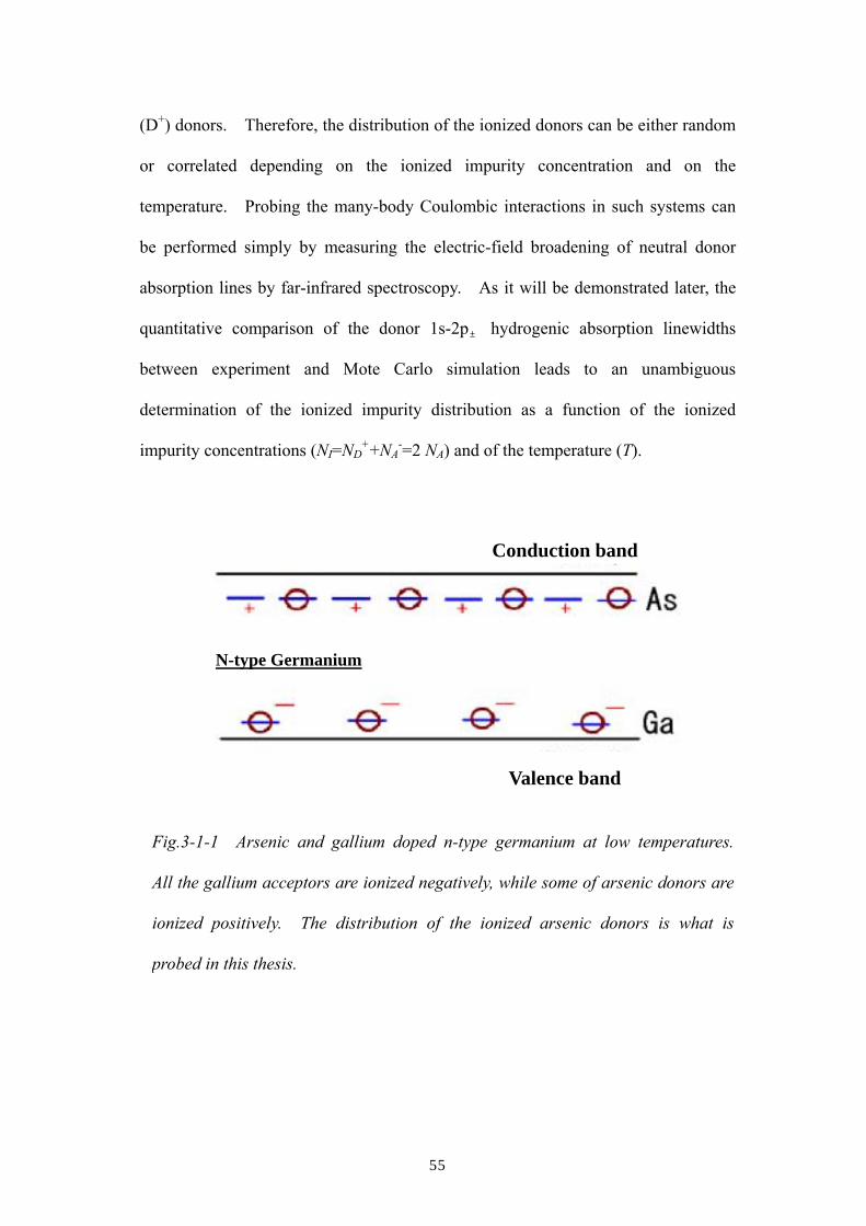
(D+) donors. Therefore, the distribution of the ionized donors can be either random
or correlated depending on the ionized impurity concentration and on the
temperature. Probing the many-body Coulombic interactions in such systems can
be performed simply by measuring the electric-field broadening of neutral donor
absorption lines by far-infrared spectroscopy. As it will be demonstrated later, the
quantitative comparison of the donor 1s-2p± hydrogenic absorption linewidths
between experiment and Mote Carlo simulation leads to an unambiguous
determination of the ionized impurity distribution as a function of the ionized
impurity concentrations (NI=ND++NA
-=2 NA) and of the temperature (T).
Conduction band
Valence band
N-type Germanium
Fig.3-1-1 Arsenic and gallium doped n-type germanium at low temperatures.
All the gallium acceptors are ionized negatively, while some of arsenic donors are
ionized positively. The distribution of the ionized arsenic donors is what is
probed in this thesis.
56
It has been expected theoretically that the ionized impurity distribution is
correlated when the available thermal energy is sufficiently smaller than the
correlation energy.2 Electrons distribute themselves among donors in such a way as
to reduce the total Coulombic energy. An energy gap is known as “Coulomb gap”
appears at the Fermi level in the density of the states of the donor band.3 The
correlation energy is of the same order of magnitude as the Coulomb energy between
Increase of Impurity Concentration Increase of temperature
Random Distribution Correlated Distribution
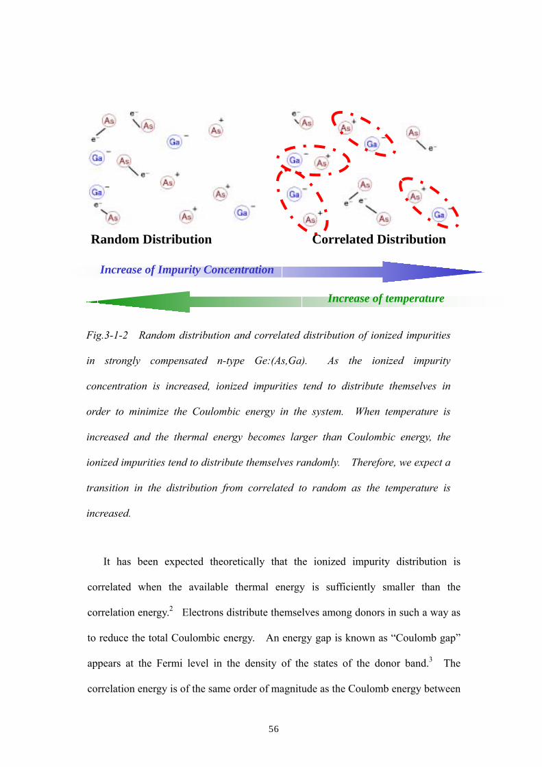
Fig.3-1-2 Random distribution and correlated distribution of ionized impurities
in strongly compensated n-type Ge:(As,Ga). As the ionized impurity
concentration is increased, ionized impurities tend to distribute themselves in
order to minimize the Coulombic energy in the system. When temperature is
increased and the thermal energy becomes larger than Coulombic energy, the
ionized impurities tend to distribute themselves randomly. Therefore, we expect a
transition in the distribution from correlated to random as the temperature is
increased.

57
impurities, e2ND1/3/κ, where κ is the dielectric constant. With NI=2KND where
K=NA/ND is the compensation ratio defined for n-type semiconductors, the correlated
distribution is expected for the condition: 2,3
3
22
eTkKNIκB≫ . (3-1-1)
For example, in the case of T=4 K, compensation ratio K=0.6, and dielectric
constant κ=16.0, the condition for the correlated distribution of ionized impurities is
( ) ].[1074.61060.1
41085.81641038.16.02 313
3
219
1223−
−
−−
×=
×
××××××× cmNI
π≫ (3-1-2)
The correlated distribution of the ionized impurities has been confirmed for the
condition given by Eq. (3-1-1) in case of p-type Ge by Itoh, et. al. previously. 1
When the thermal energy becomes larger than the correlation energy, i.e., the
left hand side of Eq. (3-1-1) is much smaller than the right hand side, electrons are
randomly distributed among donors, so that the ionized impurity distribution is
completely random. The random distribution is preferred for lower NI since the
larger distance between ions leads to weaker correlation. Larsen’s classic theory
for the calculation of the linewidth assuming the random distribution is valid for the
range; 4,5
3*5107.0 −−×≤ aNI , (3-1-3)
where a* is the effective Bohr radius of donor impurities. In case of a*=69[Å], a
value for a typical of shallow donors in Ge, the condition of completely random
58
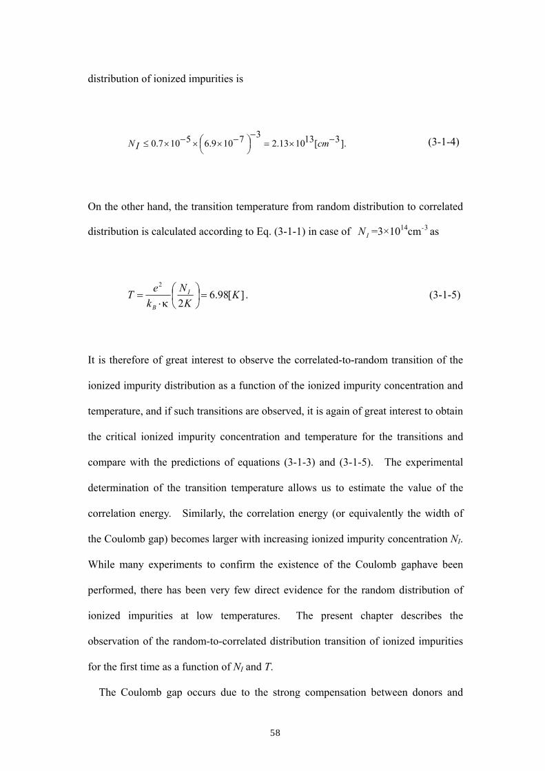
distribution of ionized impurities is
].3[131013.237109.65107.0 −×=
−
−××−×≤ cmIN (3-1-4)
On the other hand, the transition temperature from random distribution to correlated
distribution is calculated according to Eq. (3-1-1) in case of IN =3×1014cm‐3 as
][98.62
2
KK
Nk
eT I
B
=
⋅=
κ. (3-1-5)
It is therefore of great interest to observe the correlated-to-random transition of the
ionized impurity distribution as a function of the ionized impurity concentration and
temperature, and if such transitions are observed, it is again of great interest to obtain
the critical ionized impurity concentration and temperature for the transitions and
compare with the predictions of equations (3-1-3) and (3-1-5). The experimental
determination of the transition temperature allows us to estimate the value of the
correlation energy. Similarly, the correlation energy (or equivalently the width of
the Coulomb gap) becomes larger with increasing ionized impurity concentration NI.
While many experiments to confirm the existence of the Coulomb gaphave been
performed, there has been very few direct evidence for the random distribution of
ionized impurities at low temperatures. The present chapter describes the
observation of the random-to-correlated distribution transition of ionized impurities
for the first time as a function of NI and T.
The Coulomb gap occurs due to the strong compensation between donors and
59
acceptors in the system. Figure 3-1-3 schematically shows the density of states
near the donor level in cases of the compensation ratios 0, 0.1, 0.5 at the zero
temperature. As the compensation ratio is increased, the donor level splits. The
energy difference between two levels is called Coulomb gap Δ (see Eq. 3-1-6) that
corresponds to the total Coulomb energy in the system. At zero temperature, the
lower donor level is completely filled, i.e., the distribution of ionized impurities is
completely correlated. In a case of the finite temperature, some of the donor bound
electrons are excited across the gap and occupy the upper branch of the donor states.
This is an origin of the random distribution of ionized impurities in the system (Fig.
3-1-4). While this simple picture is not rigorous because smearing of the gap itself
occurs as the temperature is raised, it nevertheless provides a simple view of
defining the problem and approximate estimates of at what ionized impurity
concentration and temperature we expect the transition. The energy of the
Coulomb gap ∆ for three dimensions is approximately; 3
23210
3 κge=∆ (3-1-6)
where, κ is the dielectric constant of germanium. The density of the state near
the Fermi level 0g is estimated as
20 erKNg DDκ= , (3-1-7)
where, the average distance between donors is Dr = (3/4πND)1/3. The Coulomb
gap according to Eq. (3-1-6) and (3-1-7) is shown in Fig. 3-1-5. As one can see,
the Coulomb gap dramatically increases in the region of NI≈1013-1014 cm-3, that

60
corresponds to the ionized impurity concentrations of our set of samples as
mentioned later in Chapter 3.2.
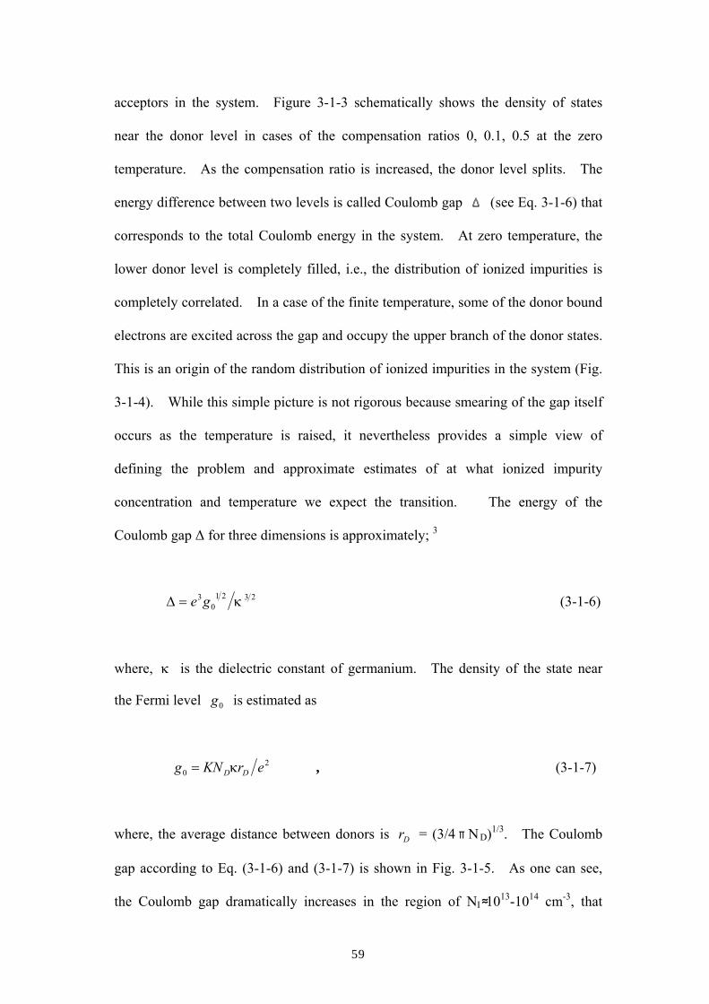
In order to obtain random-to-correlated distribution of ionized impurities, we
performed two kinds of experiments. At first, we performed the far infrared
absorption measurement as a function of the ionized impurity concentration at a
fixed temperature as shown in (1) of Fig. 3-1-6. Secondly, we determined the
impurity concentration as a function of temperature as shown in (2) of Fig. 3-1-6.
Electrons
Density of States
Energy Δ
K=0 K=0.1 K=0.5
Donor Level
Conduction Band
Fig.3-1-3 Density of states of the donor levels in cases of compensation ratio K = 0, 0.1,
and 0.5. As the compensation ratio is increased, the donor state splits due to the Coulomb
energy in the system. The lower part of the split donor levels is filled with bound electrons at
zero temperature. The energy difference between separated donor levels, Δ, is called a
“Coulomb Gap”.

61
Partially Random
Completely Random
kBT
Fig.3-1-4 Thermally induced excitation of bound electrons across the Coulomb
Gap. Electrons occupy the upper level due to temperature induced
randomization of the distribution of ionized impurities.
0
2
4
6
8
10
12
0 8 1014 1.6 1015 2.4 1015 3.2 1015
Coul
omb
Gap
[K]
Ionized Impurity Concentration [cm-3]
Fig.3-1-5 Width of the Coulomb gap according to Eq. (3-1-6) and (3-1-7).
62
Ionized Impurity Concentration
Correlated
Distribution
Random Distribution
(1)
(2)
In the past, there had been several attempts to observe distribution of ionized
impurities. A recent publication1 reported the broadening of the 1s-2p-like Ga
acceptor absorption peak in heavily compensated Ge samples having ionized
impurity concentration NI=9.0×10¹³ - 6.8×1015 cm-3. For the concentration range
they investigated, they found a better agreement with the theory based on the
correlated distribution of ionized impurities than the theory assuming a random
distribution as shown in Fig. 3-1-7. As a result of this observation, we have raised
the following questions.
1. Can we obtain same experimental results for the case of n-type samples?
(Theories dealing with the distribution of ionized impurities had been derived
for n-type samples and not for p-type that have been investigated in Ref. 1.)
2. Can we find the random distribution in low enough impurity concentration as
predicted by Eq. 3-1-1? (Only the correlated distribution was observed in Ref.
Fig. 3-1-6. An approximate phase diagram of the ionized impurity distribution.
This figure is constructed assuming the compensation ratio less than 0.9. In the
case of the compensation ratio more than 0.9, a random distribution is dominant
even when temperature is close to zero.

63
1.)
3. What is the origin of the large residual linewidth of 39 μeV in Ref. 1 in the limit
of NI =0 ?
4. Is it possible to find the random-to-correlated transition as a function of
temperature?
To answer these questions, we have prepared n-type samples that have lower
ionized impurity concentration. In order to observe random-to-correlated transition
clearly, we have prepared a large number of samples that have different ionized
impurity concentrations between 2.56×10¹³ and 2.26×1014 cm-3.
Fig. 3-1-7 A recent publication1 reporting the broadening of the 1s-2p-like Ga
acceptor absorption peak in heavily compensated Ge samples with ionized
impurity concentration NI=9.0×10¹³ - 6.8×1015 cm-3.

64
As a result we report in this thesis observation of correlated distribution for the high
impurity concentration in n-type samples. We report existence of the random
distribution for the low impurity concentrations (NI<7×1013 cm-3). We report that
the residual linewidth is due to thermal randomization of the distribution of ionized
impurities. We report on the observation of the temperature induced
random-to-correlated transition.
Before moving on to experiments, we would like to note that there is another
kind of random-to-correlated transition for large compensation ratio (K>0.7)
predicted based on my calculation described in Appendices A-E.
0
50
100
150
200
250
300
350
0 20 40 60 80 100Compensation Ratio [%]
FWH
M
Correlated distribution
Random distribution
Fig. 3-1-8. Linewidths from 1s state to 2p± state calculated when the number of
donors is 50 as a function of the compensated ratio. When the compensated ratio is
more than 90%, linewidths in case of correlated distribution are more broadened
than that of random distribution. This means the random distribution is more stable
than the correlated distribution. The detailed explanation of this calculation is
given in Appendices A and E.

65
Figure 3-1-8 shows the relation between theoretical linewidths and compensation
ratio as a result of my calculation. When the compensation ratio is less than 0.7,
the linewidths are not so strongly affected by compensation ratio, while the
linewidths in case of correlated distribution are dramatically increased as a function
of compensation ratio when compensation ratio is more than 0.8. When the
compensated ratio is more than 0.9, linewidths in case of correlated distribution is
more broadened than that of random distribution. The Coulombic energy of the
system in case of random distribution is lower than that of correlated distribution,
that is, we expect another kind of random-to-correlated distribution. Although this
type of transition is not reported in this thesis since our samples have K<0.7, it is of
great interest to observe such transition in the future.

66
3.2 Experimental Procedures
3.2.1 Samples
Samples are cut from a Cz(Czochralski)-grown, n-type Ge:(As,Ga)
single-crystal ingot as shown in Fig. 3-2-1-1. The concentrations of As and Ga
vary as a function of the position along ingot’s growth direction due to impurity
segregation during the growth as follows,
( )N x k N x k( ) = ⋅ − −0
11 , (3-2-1-1)
where, k is the segregation coefficient, N0 is the average impurity concentration, and
x is the solidification ratio. The segregation coefficients for impurities in Ge are
experimentally obtained in Table 3-2-1-1.
Fig. 3-2-1-1 The ingot we used were made by Czochralski method. The ingot
has different arsenic and gallium concentrations as a function of the position along
the growth direction as described in Fig. 3-2-1-2. The samples were cut from
different positions in order to obtain different impurity concentrations.
Seed Crystal
Germanium Ingot
Liquid Germanium

67
Table 3-2-1-1 The segregation coefficients of impurities in germanium
Impurity Segregation Coefficient
B 17
Al 0.073
Ga 0.087
In 0.001
P 0.08
As 0.02
Sb 0.003
C 0.000015
Zn 0.0004
Fig. 3-2-1-2 Germanium ingot (left illustration) and impurity concentrations
of arsenic and gallium, and the compensation ratio as a function of
solidification ratio (X) calculated according to Eq. (3-2-1-1) with the
parameters in Table 3-2-1-1.
0
1 0
0.2
0.4
0.6
0.8
1
0 0.2 0.4 0.6 0.8 1
Impu
rity
Conc
entra
tion
X
Compensation Ratio
[As] [Ga]
Position (X)
68
Figure 3-2-1-2 shows the relation between impurity concentration and
solidification ratio in the case of Ge:(As;Ga) according to Eq. (3-2-1-1) and the
segregation coefficients for As and Ga in Ge shown in Table 3-2-1-1. The impurity
concentrations at x = 0 is same as the ingot we used in this study. We obtain
samples whose impurity concentrations are systematically controlled as a function of
the position of the germanium ingot. In order to determine impurity concentrations
of our samples precisely, we have performed variable-temperature Hall effect
measurements for every sample.

69
3.2.2 Hall effect determination of the As and Ga concentrations of each
sample: procedures and results
The variable Hall effect measurement allows for precise determination of the
majority and minority impurity concentrations. In order to realize an appropriate
Hall measurement, it is required to prepare electric contacts that stay Ohmic down to
liquid helium temperatures. To obtain good electric contacts for the variable
temperature Hall measurement, we use indium (including 2% antimony) as a contact
material. By heating the sample with In(Sb) above Ge-In eutectic temperature, we
melt the contact region locally and dope heavily with Sb which is the n-type
impurities appropriate for our n-type Ge:As,Ga. The followings are the details of
the contact fabrication.
1. Polish samples with SiC slurry (# 600) to obtain flat surfaces.
2. Polish samples with smaller SiC slurry (# 1200) to reduce roughness of the
surfaces.
3. Polish etch with nitric-hydrofluoric acid (NHO3:HF=3:1) for about one minute
at room temperature.
4. Remove nitric-hydrofluoric acid by adding water to it.
5. Samples are rinsed in Hydrofluoric acid (1%) for about 15 minutes in order to
remove the surface oxides.
After etching samples, we cut indium wire (Ф=1mm), which was etched with
hydrochloric acid, with a paper cutter which was cleaned with trichloroethylene.
Indium plates (thickness is less than 0.5mm) were put on to the four corners of the
samples and pressed on. To minimize the in-plane impurity concentration
inhomogeneity within each sample, distances between electric contacts are chosen to

70
be less than 4 mm. Samples are annealed at 250˚C for five minutes in Ar gas in the
furnace illustrated in Fig. 3-2-2-1. Argon gas was used for purging inside of the
annealing furnace for over 30 minutes and its flow continues until the end of the
annealing process. As a result of this process, antimony in indium is diffused to the
samples, and the surface between the sample and indium were heavily doped as
shown in Fig. 3-2-2-1. This region is usually referred as n+ region since antimony
is a donor in germanium.
Hall effect we have been performed with a HL5500PC made by Bio-Rad Inc. The
effective magnetic field for the measurement is 0.320 T, and temperature is variable
down to about 5 K. We measure the Hall effects from room temperature to about
10 K. The bias we use for the measurement was 20µV from room temperature to
50 K, and 4µV for lower than 50 K in order to avoid resistive heating of samples.
Figure 3-2-2-2 shows the free carrier concentration n vs. 1/T for nine selected
samples measured in the van der Paw configuration. The data have been fitted
Heater
Sample
Glass cover
Figure 3-2-2-1 Illustration of the annealing furnace we used (left) and samples
after annealing (right). Temperature sensor is put under the samples.
In:Sb In:Sb n+ n+
Ge:(As;Ga)

71
very well using standard semiconductor statistics (solid curves in Fig. 3-2-2-2) with
the relation:
( )( ) ( )TkEN
nNNNnn
BDCAD
A −=−−
+ exp1β
(3-2-2-1)
where β=2 is the degeneracy factor for donors, NC is the effective density of states in
the conduction band, and ED is the ionization energy of the donors. After we obtain
ND and NA for each sample, we determine the ionized impurity concentration NI as a
function of temperature:
( ) AI NTnN 2+= . (3-2-2-2)
Fig. 3-2-2-2 Experimentally determined free carrier concentration vs.
inverse absolute temperature. The curves are the best fits to the experimental
data using Eq. (3-2-2-1) and (3-2-2-2).
5
6
7
8
9
10
11
12
13
14
15
0 0.02 0.04 0.06 0.08 0.1 0.12 0.14 0.16
Free
Car
rier
Con
cent
ratio
n [c
m-3
]
1/Temperature [K -1]
10
10
10
10
10
10
10
10
10
10
10
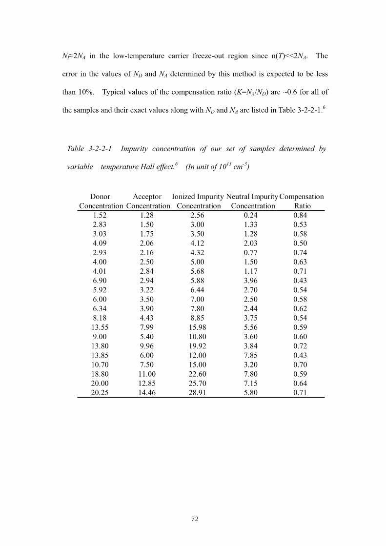
72
NI≈2NA in the low-temperature carrier freeze-out region since n(T)<<2NA. The
error in the values of ND and NA determined by this method is expected to be less
than 10%. Typical values of the compensation ratio (K=NA/ND) are ~0.6 for all of
the samples and their exact values along with ND and NA are listed in Table 3-2-2-1.6
Table 3-2-2-1 Impurity concentration of our set of samples determined by
variable temperature Hall effect.6 (In unit of 1013 cm-3)
Donor Acceptor Ionized Impurity Neutral Impurity CompensationConcentration Concentration Concentration Concentration Ratio
1.52 1.28 2.56 0.24 0.842.83 1.50 3.00 1.33 0.533.03 1.75 3.50 1.28 0.584.09 2.06 4.12 2.03 0.502.93 2.16 4.32 0.77 0.744.00 2.50 5.00 1.50 0.634.01 2.84 5.68 1.17 0.716.90 2.94 5.88 3.96 0.435.92 3.22 6.44 2.70 0.546.00 3.50 7.00 2.50 0.586.34 3.90 7.80 2.44 0.628.18 4.43 8.85 3.75 0.5413.55 7.99 15.98 5.56 0.599.00 5.40 10.80 3.60 0.6013.80 9.96 19.92 3.84 0.7213.85 6.00 12.00 7.85 0.4310.70 7.50 15.00 3.20 0.7018.80 11.00 22.60 7.80 0.5920.00 12.85 25.70 7.15 0.6420.25 14.46 28.91 5.80 0.71

73
3.3 Results and discussion
Figure 3-3-1 (a) shows a raw spectrum of Ge:(As;Ga) measured at 4 K. The
absorption peak is assigned as the transition from the ground state to the 2p± excited
state. The background of Fig. 3-3-1 (a) is due to multi-phonon absorption since
single phonon absorption cannot be observed by absorption measurements. The
absorption spectrum in Fig. 3-3-1 (b) has been obtained after subtraction of the
background.
One notices small fringes on the both sides of the absorption peak at 100 cm-1, which
is due to the effect of Apodization function. We used a BOXCAR function for
apodizing. The spectrum apodized with a BOXCAR function is not broadened, but
92 96 100 104 108 112 116 120
Fig.4-2-3 試料1の透過光スペクトル
波数 [cm-1 ]Wavenumber [cm-1] 0
1
2
3
4
5
6
7
98 99 100 101 102 103
Fig.4-2-4 試料1 As 1s→2p±光吸収スペクトルと
そのローレンツ・フィッティング
波数 [cm -1]Wavenumber [cm-1]
Fig. 3-3-1 (a) Raw spectrum of Ge:(As;Ga) measured at 4 K. The absorption at
100 cm-1 is assigned to 1s-2p± line. (b) Absorption spectrum of Ge:(As;Ga)
measured at 4 K. The absorption at 100 cm-1 is assigned to 1s-2p± line. Solid line
is the best fit with Lorentzian.

74
fringe appears at the both sides as described in Chapter 2. Therefore, imperfect
agreement of the fit to the both sides of the absorption peak at 100 cm-1 is of no
concern. The agreement of the fitting to the main part of the absorption peak is
excellent. Therefore, we obtain linewidths (FWHM) of samples with very high
precision.
99.8 100.0 100.2 100.4 100.6 100.8 101.0
3p±
2p±
2p0
75 80 85 90 95 100 105 110-202468
101214
Abs
orpt
ion
Coe
ffic
ient
[cm
-1]
Wavenumber [cm-1]
Abs
orpt
ion
Coe
ffici
ent [
a. u
.]
Wavenumber [cm-1]
Fig. 3-3-2 An inset shows As donor absorption peaks recorded at T=4 K with a
sample having NI= 3.50×1013cm-3. The three absorption peaks correspond to the
1s-2p0 (76 cm-1), 1s-2p± (100 cm-1), and 1s-3p± (106 cm-1) transitions. The main
frame shows the enlargement of the 1s-2p± (100 cm-1) absorption peak determined
experimentally (), calculated assuming random () and correlated (∆) distributions
of ionized impurities using the Monte Carlo method. Solid curves are the best fits to
the experimental and calculated points assuming Lorentzian distributions.

75
The inset of Fig. 3-3-2 shows the absorption spectrum of a sample having
ND=3.03×1013cm-3, NA=1.75×1013cm-3, i.e., NI≈2NA=3.50×1013 cm-3. It has been
recorded at T = 4 K with a resolution of 0.026 cm-1 in the wavenumber range
between 70 and 110 cm-1. Three distinct peaks correspond to excitations of bound
electrons of As in Ge from ground state to 2p0, 2p±, and 3p± excited states,
respectively. The main frame of Fig. 3-3-2 shows from bottom to top the
enlargement of the 1s to 2p± transition peaks; the experimental result (open circles),
Monte Carlo simulation assuming random distribution of ionized impurities (open
squares), and Monte Carlo simulation assuming correlated distribution of impurities
(open triangles). The Monte Carlo simulations are based on the theoretical
calculation reported in Eq. (25) of Ref. 5, which is used for isotropic conduction
bands of GaAs. We re-calculated it for anisotropic conduction band for Ge using
Faulkner’s method which is based on Kohn-Luttinger’s method.7,8 Details of the
calculation of an anisotropic conduction band and Monte Carlo simulation we used
are described in Appendix A and E. The solid curves are Lorentzian fits to each set
of data.
Fig. 3-3-3 shows FWHM vs. NI at T = 4 K. The experimental data (filled
circles) are compared with the theoretical linewidths assuming random (dashed line)
and correlated (solid line) distributions of ionized impurities. The intrinsic
linewidth due to phonon lifetime broadening9 for Ge has been found experimentally
to be 0.066 cm-1 10, i.e., it is negligibly small compared to the linewidths shown in
Fig. 3-3-4. Also ND<1× 1015 cm-3 for all of the samples employed, i.e., the
broadening due to overlap of donor wavefunctions (concentration broadening) is
negligible with respect to the amount of electric field broadening.11 Therefore, it is
appropriate to compare the experimentally found FWHM directly to the calculation
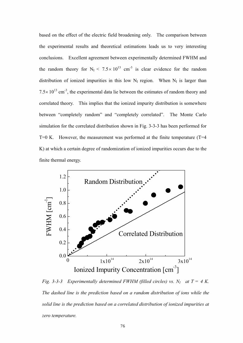
76
based on the effect of the electric field broadening only. The comparison between
the experimental results and theoretical estimations leads us to very interesting
conclusions. Excellent agreement between experimentally determined FWHM and
the random theory for NI < 7.5 × 1013 cm-3 is clear evidence for the random
distribution of ionized impurities in this low NI region. When NI is larger than
7.5×1013 cm-3, the experimental data lie between the estimates of random theory and
correlated theory. This implies that the ionized impurity distribution is somewhere
between “completely random” and “completely correlated”. The Monte Carlo
simulation for the correlated distribution shown in Fig. 3-3-3 has been performed for
T=0 K. However, the measurement was performed at the finite temperature (T=4
K) at which a certain degree of randomization of ionized impurities occurs due to the
finite thermal energy.
Fig. 3-3-3 Experimentally determined FWHM (filled circles) vs. NI at T = 4 K.
The dashed line is the prediction based on a random distribution of ions while the
solid line is the prediction based on a correlated distribution of ionized impurities at
zero temperature.
0 1x10¹⁴ 2x10¹⁴ 3x10140.0
0.2
0.4
0.6
0.8
1.0
1.2
Correlated Distribution
Random Distribution
FWH
M [c
m-1]
Ionized Impurity Concentration [cm-3]
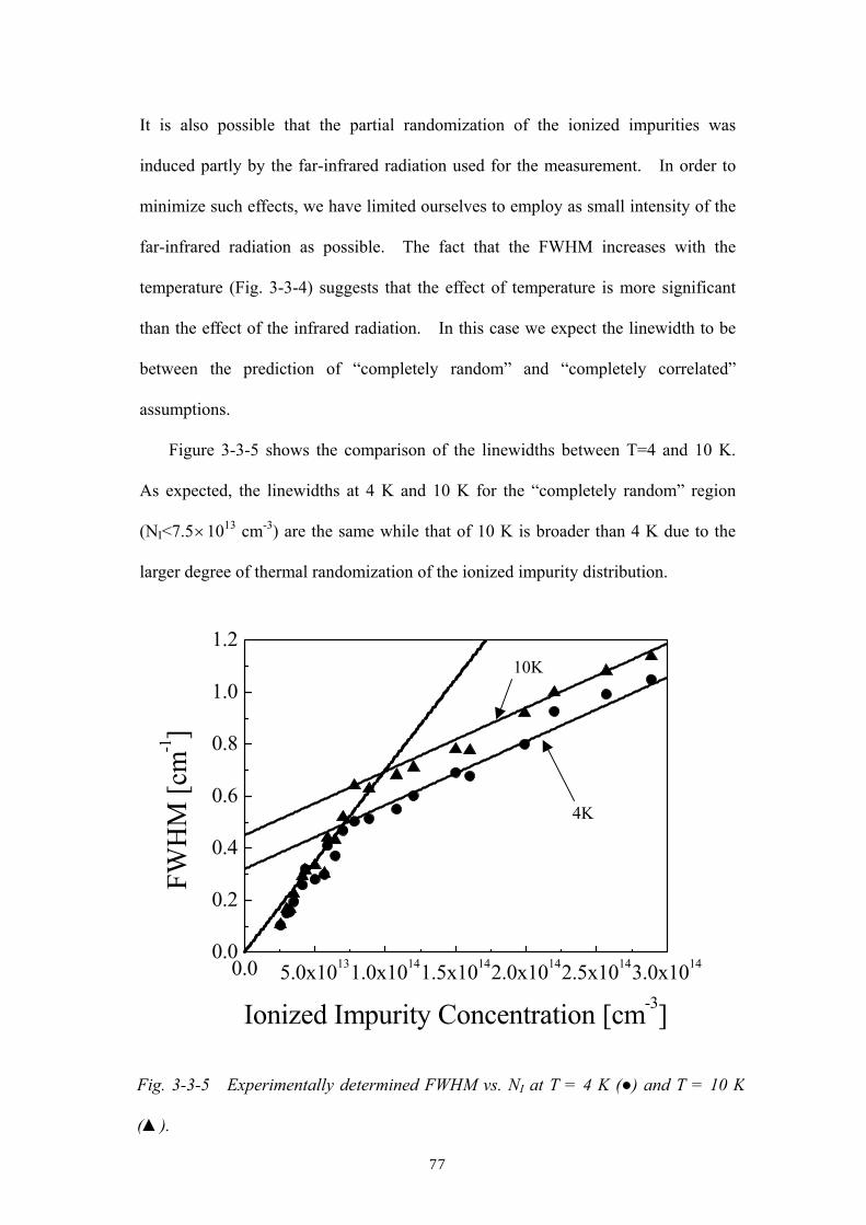
77
It is also possible that the partial randomization of the ionized impurities was
induced partly by the far-infrared radiation used for the measurement. In order to
minimize such effects, we have limited ourselves to employ as small intensity of the
far-infrared radiation as possible. The fact that the FWHM increases with the
temperature (Fig. 3-3-4) suggests that the effect of temperature is more significant
than the effect of the infrared radiation. In this case we expect the linewidth to be
between the prediction of “completely random” and “completely correlated”
assumptions.
Figure 3-3-5 shows the comparison of the linewidths between T=4 and 10 K.
As expected, the linewidths at 4 K and 10 K for the “completely random” region
(NI<7.5×1013 cm-3) are the same while that of 10 K is broader than 4 K due to the
larger degree of thermal randomization of the ionized impurity distribution.
Fig. 3-3-5 Experimentally determined FWHM vs. NI at T = 4 K () and T = 10 K
().
0.0 5.0x10131.0x10141.5x10142.0x10142.5x10143.0x10140.0
0.2
0.4
0.6
0.8
1.0
1.2
FWH
M [c
m-1]
Ionized Impurity Concentration [cm-3]
10K
4K

78
The critical ionized impurity concentration (NIC), where the change of slope occurs
in Fig. 3-3-5, shifts from 7.5×1013 cm-3 at T=4 K to approximately 1.0×1014 cm-3 at
T=10 K. Lee et al. have shown for Si:B that the Coulomb gap smears out with
increasing temperature due to increasing population of above-gap states.12 Our
observation of the increasing NIC and FWHM above NIC with T is consistent with
what has been shown for Si:B. Figure 3-3-6 shows the temperature dependence of
the FWHM () for a sample having NI=7.8×1013 cm-3, which is just above the
critical concentration NIC=7.5×1013 cm-3 for T=4 K.13-15 We are interested in
whether we observe random to correlated transition with increasing temperatures
from T=2 K. Figure 3-3-6 shows clearly that the FWHM increases in two steps; the
first gradual increase occurs between T=5 and 11 K and the second rapid increase
takes place above T=14 K. The second increase at T>14 K is due to thermal
ionization of donors as it matches with the increment of NI (solid curve) calculated
using Eqs. (3-2-2-1) and (3-2-2-2). The first gradual increase is due to the
transition of the ionized impurity distribution from correlated to random, and the two
plateaus in FWHM at T=2-5 K and T=11-13 K represent characteristic FWHM for
the two distributions. In order to support our claim that we have observed the
transition, we shall estimate the critical temperature (Tc) for the transition using the
theory of Efros and Shklovskii3 and compare the result directly with our
experimental observation. Using Eqn. (3-1-6) and (3-1-7), the Coulomb gap
∆=0.31 meV has been obtained for the sample having NI=7.8×1013 cm-3 in Fig.
3-3-6. To first order, we expect Tc to be of the same order as ∆, i.e., Tc≈3.6 K is
what we estimate based on theory. The experimentally found gradual increase
starts around 4 K, in very good agreement with the theoretically estimated Tc≈3.6 K.
The inset in Fig. 3-3-6 shows the temperature dependence of the FWHM for samples
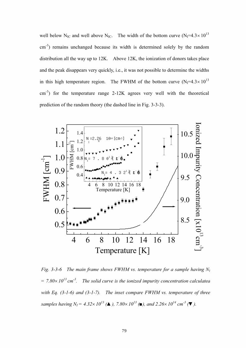
79
well below NIC and well above NIC. The width of the bottom curve (NI=4.3×10¹³
cm-3) remains unchanged because its width is determined solely by the random
distribution all the way up to 12K. Above 12K, the ionization of donors takes place
and the peak disappears very quickly, i.e., it was not possible to determine the widths
in this high temperature region. The FWHM of the bottom curve (NI=4.3×10¹³
cm-3) for the temperature range 2-12K agrees very well with the theoretical
prediction of the random theory (the dashed line in Fig. 3-3-3).
4 6 8 10 12 14 16 18
0.50.60.70.80.91.01.11.2
Ionized Impurity C
oncentration [x10 13cm-3]
10.5
10.0
9.5
9.0
-
-
-
-
8.5-
FWH
M [c
m-1]
Temperature [K]
4 6 8 10 12 14 16 18
0.4
0.6
0.8
1.0
1.2
1.4
NI=4.32×10¹³[cm-3]
NI=7.80×10¹³[cm-3]
NI=2.26 ×10
14[cm-3]
FWH
M [c
m-1]
Temperature [K]
Fig. 3-3-6 The main frame shows FWHM vs. temperature for a sample having NI
= 7.80×1013 cm-3. The solid curve is the ionized impurity concentration calculated
with Eq. (3-1-6) and (3-1-7). The inset compare FWHM vs. temperature of three
samples having NI = 4.32×10¹³ (), 7.80×10¹³ (), and 2.26×1014 cm-3 ().

80
The FWHM of the top curve in the inset (NI=2.26×1014 cm-3) for the temperature
range shown is determined dominantly by the correlated distribution because the
donor concentration is high enough for the neighboring ionized impurities to interact
with one another. The FWHM increases with the increasing temperature because
the partial randomization of the correlated distribution proceeds as was shown in Fig.
3-3-7.
Observation of the random-correlated transition of ionized impurity
distributions as a function of temperature has been claimed before by Baranovskii et
al. for GaAs.16,17 However, the calculational result from Eq. (3-2-2-1) and
(3-2-2-2) shows they did not observed the transition of the ionized impurities.
Fig. 3-3-7 Temperature dependence of the free carrier concentration calculated
from Eq. (3-2-2-1) and (3-2-2-2). The increase of the ionized impurities is due to
that of the free carriers, i.e., the rapid increase of the linewidths in the range of high
temperature (about < 10 K) in Fig. 3-3-6 is due not to the transition of the
distribution of ionized impurities.
0 5 10 15 20
NI=2.26×10¹⁴ [cm-3]の試料
NI=7.80×10¹³ [cm-3]の試料
NI=4.32×10¹³ [cm-3]の試料
Car
rier C
once
ntra
tion
[a. u
.]
Tempereture [K]

81
Figure 3-3-7 shows the temperature dependence of the free carrier concentration
corresponding to that of ionized impurities. Additionally, our analysis of their data
shows that they observe increase of FWHM due to ionization of donors and not the
transition. As one can see in the inset of Fig. 3-3-6, it takes extreme fine-tuning of
ND and NA in order to observe a clear signature of the transition with two distinct
plateaus below the temperatures where ionization takes place. The precise control
of both donors and acceptors at the level of 1013 cm-3 has been the key for the
successful observation of random-to-correlated transition of the ionized impurity
distribution in semiconductors.

82
References
1 K. M. Itoh, J. Muto, W. Walukiewicz, J. W. Beeman, E. E. Haller, Hyunjung Kim,
A. J. Mayur, M. Dean Sciacca, A. K. Ramdas, R. Buczko, J. W. Farmer, and V. I.
Ozhogin, Phys. Rev. B 53, 7797 (1996).
2 S. M. Kogan and N. Van Lien, Fiz. Tekh. Poluprovodn. 15, 44 (1981) [Sov. Phys.
Semicond. 15, 26 (1981)].
3 B.I.Shklovskii and A.L.Efros, in Electronic Properties of Doped Semiconductors,
(Springer-Verlag, Berlin Heidelberg New York Tokyo, 1984), Vol. 45, p.237.
4 D. M. Larsen, Phys. Rev. B 8, 535 (1973).
5 D. M. Larsen, Phys. Rev. B 13, 1681 (1976).
6 J. Kato, K. M. Itoh, and E. E. Haller, Physica B, 301-302, 1 (2001).
7 W. Kohn and J. M. Luttinger, Phys. Rev. 98, 915 (1955).
8 R. A. Faulkner, Phys. Rev. 184, 713 (1969).
9 K. Nishikawa and R. Barrie, Can. J. Phys. 41, 1135 (l963); R. Barrie and K.
Nishikawa, Can. J. Phys. 41, 1823 (1963).
10 H. Navarro, E. E. Haller, and F. Keilmann, Phys. Rev. B 37, 10822 (1988).
11 W. Baltensperger, Philos. Mag. 44, 1355 (1953).
12 Mark Lee, J. G. Massey, V. L. Nguyen, and B. I. Shklovskii, Phys. Rev. B 60,
1582 (1999).
13 Jiro Kato, Kohei M. Itoh, and Eugene E. Haller, Physica B, 308-310 521 (2001).
14 Jiro Kato, Kohei M. Itoh, and Eugene E. Haller, Phy. Rev. B 65 241201-1
(2002).
15 J. Kato and K. M. Itoh, Journal of the Physical Society of Japan Supplement, in
press.

83
16 S. D. Baranovskii, B. L. Gel’mont, V. G. Golubev, V. I. Ivanovskii, and A. V.
Osutin, Pis’ma Zh. Eksp. Teor. Fiz. 46, 405 (1987) [JETP Lett. 46, 510 (1987)].
17 S. D. Baranovskii, B. L. Gel’mont, V. G. Golubev, V. I. Ivanovskii, and A. V.
Osutin, Fiz. Tekh. Poluprovodn. 23, 1434 (1989) [Sov. Phys. Semicond. 23, 891
(1989)].
84
Chapter 4: The host isotope effect on the local vibrational modes
of oxygen in isotopically enriched crystalline 28Si, 29Si and 30Si
4.1 Introduction
A wide variety of novel isotope effects have been discovered recently1-5,
thanks to the availability of high quality bulk Si crystals with controlled isotopic
compositions.6, 7 In contrast to well-behaved isotope effects on phonons in Si
crystals with relatively mixed isotopic compositions,2 unpredictable isotope effects
have been discovered more recently in nearly 100% mono-isotopic Si crystals.3-5
With respect to the results obtained with natural silicon (hereafter natSi) that
composed of the isotopic composition 28Si (92.23%), 29Si (4.67%), and 30Si (3.10%),
a dramatic increase of the thermal conductivity3, a significant narrowing of the
impurity bound exciton luminescence peaks4, and absence of the acceptor ground
state splitting5 have been found unexpectedly when the enrichment of 28Si exceeded
99.98%. Similarly, a surprisingly large isotope effect on hydrogenic impurity levels
has been reported for isotopically enriched diamond.8 The present paper reports on
another intriguing effect of isotopes observed on the localized vibrational mode
(LVM) of impurity oxygen in Si.
Because of its technological importance, behaviors of oxygen in silicon have
been studied extensively.9 As a result, rich physics associated with the localized
motion of light impurities embedded in a relatively heavy host matrix has been
revealed using oxygen in Si as one of ideal examples. An oxygen atom in silicon
tends to exist as an interstitial defect between two silicon atoms at off-center
positions in the 〈111〉 direction as shown in Fig. 3-1-1.9-14 Ab initio calculations

85
have shown the bond lengths of Si-O to be 1.59Å with the Si-O-Si bond angle
172°.15 An interstitial oxygen atom has two equivalent nearest neighbor Si atoms,
six equivalent second nearest neighbor Si atoms, eighteen equivalent third neighbor
Si atoms, and so on. In the framework of the harmonic approximation, frequencies
of oxygen in silicon are determined by the local structures and masses (i.e., isotopes)
of vibrating oxygen and neighboring Si atoms.16 In many cases the isotope shifts of
the spring constants k and K of Si-O and Si-Si bonds, respectively, are small enough
to be ignored.
2nd nearest-neighbor Si
2nd nearest-neighbor Si
1st nearest-neighbor Si
1st nearest-neighbor Si
Interstitial Oxygen
K K
K
K K K
k
k
Fig. 4-1-1. The illustration of an interstitial oxygen atom in Si crystals. Oxygen
atom locates off-centered position between two neighboring silicon atoms. There
are three stable isotopes of oxygen (16O, 17O, 18O) and three silicon isotopes (28Si,
29Si, 30Si).

86
Therefore, isotope substitution of the oxygen centers with 16O, 17O, and 18O,
which changes exclusively the mass of vibrating species, has been useful in the past
for experimental understanding of the LVM of oxygen in Si. Moreover, the
discovery of the LVM linewidth of 17O being a factor of 1.5 larger than those of 16O
and 18O has suggested strongly that the interaction between Si phonons and oxygen
LVMs determines the linewidth of the oxygen LVMs in Si.14,20,21 In order to
understand the interaction between the bulk Si isotopes and vibrating oxygen atoms,
two factors must be considered separately;
i) energy dependence of the phonon density of states which is determined mainly by
the average mass of the constituting Si isotopes and
ii) disorder in Si masses (disorder in Si isotope distribution) which arises from the
co-presence of 28Si, 29Si, and 30Si isotopes.
While the larger linewidth of 17O is most likely due to the former effect, the effect of
isotopic disorder is predicted to be negligibly small within the framework of the
harmonic approximation as we will show later. As a result, the LVM linewidth is
believed to be determined solely by the relation between the LVM frequency (that
depends on the masses of the oxygen and neighboring Si) and the density of the
phonon states of Si. However, recent pump and probe measurements of oxygen
LVM in Si revealed the LVM lifetime of 229 ps which translates to the width of
0.023 cm-1,17 i.e., the linewidth measured in the absorption measurement may be
inhomogeneously broadened.
A calculation focusing on the mass of the vibrating oxygen and its two nearest
neighbors describe the energies of the LVMs to the first order. Theory of LVM of

87
oxygen in silicon proposed by Yamada-Kaneta et al. has been in good agreement
with the experimental results for a variety of modes.10-14 His quantum mechanical
calculation has separated the oxygen vibration perpendicular to the [111] plane from
the ones parallel to the [111] plane. Directions of vibrations of the A1g and A2u
modes are parallel to〈111〉 axis, while those of 2D LEAE (two-dimensional
low-energy anharmonic excitation,13 also known as low-frequency mode14 or 29 cm-1
mode10-12) are perpendicular to 〈111〉axis, as shown in Fig. 4-1-2. Energy
diagrams of the three major LVM modes and IR allowed transitions are shown in Fig.
4-1-3. Here N and M represent the contributions of the vibration due to A2u and
A1g modes, respectively, l is the angular moment along to 〈111〉 direction, and k is
the integers to distinguish each energy state.
2D LEAE A1g A2u
Fig. 4-1-2 The vibrational modes of the interstitial oxygen (red spheres) embedded in a
silicon crystal (gray spheres). There are A2u, A1g and Eu modes for the case of 2Cv
symmetry. The Eu modes are known as 2D LEAE (two-dimentional low-energy
anharmonic excitation) in the case of the LVMs of oxygen in silicon, since the interstitial
oxygen atoms are located at off center position between silicon atoms.

88
The calculation performed by Yamada-Kaneta et al. has explained not only the LVM
lines between zero-point energies of each mode but also those between non
zero-point energies. It has been developed based on the masses of vibrational
oxygen and its two nearest neighbor host atoms.
The present paper reports on the surprisingly large effect of Si isotopic mass
disorder on the oxygen LVM linewidths, which cannot be explained at all by the
harmonic approximation. Similar to the case of the recent experiments on oxygen
LVMs in isotopically controlled Ge,18, 19 the present work has investigated LVMs of
oxygen in Si samples with controlled isotopic composition.
Fig. 4-1-3 Theoretically obtained discrete energy states of the LVMs of oxygen in
silicon.14, 20-22 N and M indicate the contributions of A2u and A1g modes, respectively, l
is the angular moment along <111> directions, and k is the integers to distinguish each
energy state. (Illustration taken from Ref.14. )
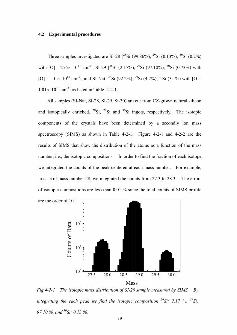
89
4.2 Experimental procedures
Three samples investigated are SI-28 [28Si (99.86%), 29Si (0.13%), 30Si (0.2%)
with [O]= 4.75×1017 cm-3], SI-29 [28Si (2.17%), 29Si (97.10%), 30Si (0.73%) with
[O]= 1.01×1018 cm-3], and SI-Nat [28Si (92.2%), 29Si (4.7%), 30Si (3.1%) with [O]=
1.01×1018 cm-3] as listed in Table. 4-2-1.
All samples (SI-Nat, SI-28, SI-29, Si-30) are cut from CZ-grown natural silicon
and isotopically enriched, 28Si, 29Si and 30Si ingots, respectively. The isotopic
components of the crystals have been determined by a secondly ion mass
spectroscopy (SIMS) as shown in Table 4-2-1. Figure 4-2-1 and 4-2-2 are the
results of SIMS that show the distribution of the atoms as a function of the mass
number, i.e., the isotopic compositions. In order to find the fraction of each isotope,
we integrated the counts of the peak centered at each mass number. For example,
in case of mass number 28, we integrated the counts from 27.3 to 28.3. The errors
of isotopic compositions are less than 0.01 % since the total counts of SIMS profile
are the order of 106.
27.5 28.0 28.5 29.0 29.5 30.0104
105
106
Cou
nts
of D
ata
MassFig.4-2-1 The isotopic mass distribution of SI-29 sample measured by SIMS. By
integrating the each peak we find the isotopic composition 28Si: 2.17 %, 29Si:
97.10 %, and 30Si: 0.73 %.

90
Isotopic composition of SI-28 as published in Ref. 7 was also obtained by the SIMS
measurement. The oxygen concentration of natural silicon has been determined by
the LVM absorbance of 1100 cm-1 line at 77 K and 300 K. We used the American
Standard for Testing and Materials F121-79 for deciding the oxygen concentration in
natural silicon. In order to determine the oxygen concentration, we use the ratio of
the intensities of the main peak at 1100 cm-1 and the baseline at the shoulders of the
main peak. In case SI-29 sample, the transmittance (T) of the base line is 0.42 and
transmittance at the peak is 0.26. With the refractive index of silicon crystal
n=4.298 and the sample thickness d=0.07 cm, the reflection value R=10.9 is obtained
by the relation,
( )21−= nR . (4-2-1)
27.5 28.0 28.5 29.0 29.5 30.0 30.5
105
106
107
Cou
nts o
f Dat
a
Mass
Fig.4-2-2 The isotopic mass distribution of SI-30 crystal measured by SIMS. The
isotopic composition of the sample is 28Si:0.67%, 29Si: 0.59%, and 30Si: 98.74%.
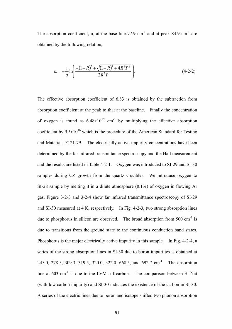
91
The absorption coefficient, α, at the base line 77.9 cm-1 and at peak 84.9 cm-1 are
obtained by the following relation,
( ) ( )
+−+−−−=
TRTRRR
d 2
2242
2411
ln1α . (4-2-2)
The effective absorption coefficient of 6.83 is obtained by the subtraction from
absorption coefficient at the peak to that at the baseline. Finally the concentration
of oxygen is found as 6.48x1017 cm-3 by multiplying the effective absorption
coefficient by 9.5x10¹⁶ which is the procedure of the American Standard for Testing
and Materials F121-79. The electrically active impurity concentrations have been
determined by the far infrared transmittance spectroscopy and the Hall measurement
and the results are listed in Table 4-2-1. Oxygen was introduced to SI-29 and SI-30
samples during CZ growth from the quartz crucibles. We introduce oxygen to
SI-28 sample by melting it in a dilute atmosphere (0.1%) of oxygen in flowing Ar
gas. Figure 3-2-3 and 3-2-4 show far infrared transmittance spectroscopy of SI-29
and SI-30 measured at 4 K, respectively. In Fig. 4-2-3, two strong absorption lines
due to phosphorus in silicon are observed. The broad absorption from 500 cm-1 is
due to transitions from the ground state to the continuous conduction band states.
Phosphorus is the major electrically active impurity in this sample. In Fig. 4-2-4, a
series of the strong absorption lines in SI-30 due to boron impurities is obtained at
245.0, 278.5, 309.3, 319.5, 320.0, 322.0, 668.5, and 692.7 cm-1. The absorption
line at 603 cm-1 is due to the LVMs of carbon. The comparison between SI-Nat
(with low carbon impurity) and SI-30 indicates the existence of the carbon in SI-30.
A series of the electric lines due to boron and isotope shifted two phonon absorption

92
lines in SI-30 are shown in Fig. 4-2-5. Again a signature of the high concentration
of carbon is found near the TO+TA phonon line. The dip at 510 cm-1 is probably
due to the electric transition of impurities, since the peak has a temperature
dependence characteristic of the electronic transitions. The carbon concentration in
SI-30 is estimated to be 5.07×1017 cm-1 by these observations. This value was
obtained by the method described in Ref. 9. The infrared absorption spectra were
recorded with a BOMEM DA-8 Fourier transform spectrometer with a Globar light
source, a KBr beam splitter, and MCT detector. The resolution was 0.03 cm-1 and
the signal-to-noise ratio was improved by coadding 200 spectra. The samples were
cooled in an OXFORD OPTISTAT cryostat with a ZnSe window and the sample
temperature was monitored with a calibrated thermometer installed at the sample
mount.
Fig. 4-2-3 Far infrared spectroscopy of SI-29 measured at 4 K. Strong absorptions
at 278 and 319 cm-1 correspond to the electronic absorptions of phosphorus.
100 200 300 400 500 600
4
5
6
7
8
Phosphorus lines
Abs
orpt
ion
Coe
ffic
ient
[cm-1
]
Wave Number [cm-1]

93
Fig. 4-2-4 Temperature dependence of far infrared absorption spectroscopy of
SI-30. A series of the strong absorptions indicate the electronic transitions due to
boron. The absorption line at 603 cm-1 is due to the LVMs of carbon.
200 300 400 500 600 70015.0
15.5
16.0
16.5
17.0
17.5
18.0
18.5LVM of 12C in 30Si
Boron lines
Abs
orba
nce
[cm
-1]
Wavenumber [cm-1]
004K 010K 020K 040K 060K 080K 100K 120K 150K 200K 250K
200 300 400 500 600 700
15.0
17.5
T = 4 [K]
Two phonon (TO+TA)
LVM of C
Boron lines
NatSi(low [C])
30Si(high [C])
Abs
orba
nce
[cm
-1]
Wavenumber [cm -1]
Figure 4-2-5 Comparison between SI-Nat and SI-30 measured at 4 K. Strong
absorptions arise due to boron and two-phonon absorption in both samples.
Features due to carbon are observed only in SI-30.
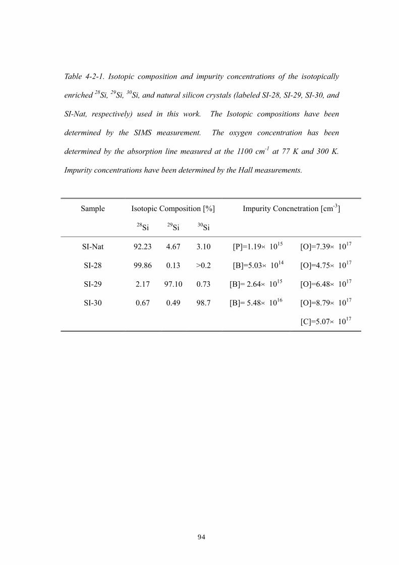
94
Table 4-2-1. Isotopic composition and impurity concentrations of the isotopically
enriched 28Si, 29Si, 30Si, and natural silicon crystals (labeled SI-28, SI-29, SI-30, and
SI-Nat, respectively) used in this work. The Isotopic compositions have been
determined by the SIMS measurement. The oxygen concentration has been
determined by the absorption line measured at the 1100 cm-1 at 77 K and 300 K.
Impurity concentrations have been determined by the Hall measurements.
Isotopic Composition [%] Impurity Concnetration [cm-3] Sample
28Si 29Si 30Si
SI-Nat 92.23 4.67 3.10 [P]=1.19×10¹⁵ [O]=7.39×10¹⁷
SI-28 99.86 0.13 >0.2 [B]=5.03×10¹⁴ [O]=4.75×10¹⁷
SI-29 2.17 97.10 0.73 [B]= 2.64×10¹⁵ [O]=6.48×10¹⁷
SI-30 0.67 0.49 98.7 [B]= 5.48×10¹⁶ [O]=8.79×10¹⁷
[C]=5.07×10¹⁷

95
4.3 Results and discussion
Experimental data and discussions will be presented in the following three
sub-sections as follows.
(i) Sec. 4.3.1. The effect of the nearest Si atoms on oxygen LVM. A harmonic
linear chain model is used successfully for the discussion.
(ii) Sec. 4.3.2. The effect of the 2nd and beyond nearest-neighboring Si atoms.
The harmonic model is used for the discussion with a partial success.
(iii) Sec. 4.3.3. The effect of host Si atoms on LVM linewidths of oxygen in
SI-Nat, SI-28, and SI-29. The breakdown of the harmonic model will be
discussed.
4.3.1. Effect of 1st nearest-neighboring host silicon atoms
Figure 4-3-1-1 shows the A2u-related absorption spectrum of the SI-29 sample
obtained at 4 K. The inset shows an energy diagram of the A2u-related excitations
based on the notation |N,l,k〉 that has been employed in Ref. 13, 20-22. Here N, l,
and k are the principal quantum number of the A2u mode, the angular momentum of
the oxygen around the 〈 111 〉 axis, and the additional quantum number
distinguishing the states of the same N and l, respectively. Values of the energy
separation shown in the inset are calculated for the 29Si-16O-29Si configuration based
on a harmonic model of a linear chain composed of one linear 29Si-16O-29Si molecule
surrounded by 196 Si atoms of the average mass 28.966 which is in accordance with
the isotopic composition of SI-29. The periodic boundary condition is imposed to
eliminate the dangling bonds. The bonding constant connecting two Si atoms is

96
kSi-Si=Mω2/4= 113.3 N/m, where M is the mass of Si atoms and ω = 524.6 cm-1 is the
TO phonon energy at the Γ point determined by Raman spectroscopy of isotopically
pure Si.4 The bonding constant between Si and oxygen, kSi-O= 479.18 N/m, is
determined from the frequency of the A2u mode of 28Si-16O-28Si calculated by
Yamada-Kaneta et. al. (1151.5 cm-1).20-22 Details of this calculation is explained at
the end of this chapter in the case of five atom model, and the calculational code is
shown in Appendix V. We assume the same spring constants kSi-Si and kSi-O for the
all combinations of Si and O isotopes. A strong line at 1132.5 cm-1 observed
experimentally in the mainframe of Fig. 4-3-1-1 is the A2u excitation from the |0,0,0〉
to |1,0,0〉 states of the 29Si-16O-29Si configuration, which agrees very well with the
estimation of the harmonic model shown in the inset. Figure 4-3-2 also shows
several other LVM lines. The line at 1081.0 cm-1 is due to |0,0,0〉-|1,0,0〉 of
29Si-18O-29Si, 1201.4 cm-1 is |0,0,0〉 -|1,1,0〉 of 29Si-16O-29Si, 1207.7 cm-1 is
10,0,± - 11,1,± of 29Si-16O-29Si, 1100.6 cm-1 is most likely carbon-oxygen
complexes previously reported at 1103.9 cm-1 in natSi 23, and 1047.2 cm-1 may be
related to the oxygen-impurity complexes discussed by Chappell et al..24 In addition,
a LVM line due to the A2u+A1g combined mode of 29Si-16O-29Si is observed at
1734.4cm-1 in Fig. 4-3-1-3. The direct comparison of the peak positions between
experiment and calculations are in excellent agreement as shown in Table 4-3-1.
Figure 4-3-1-2 shows the temperature dependence of the 1132.5 cm-1 excitation.
As the temperature is raised, the low-frequency states such as 2D LEAE are excited.
Therefore, the absorption intensities of the peaks at 1118.3 cm-1 ( 20,0,± - 21,0,±
of 29Si-16O-29Si ), 1124.5 cm-1 ( 10,0,± - 11,0,± of 29Si-16O-29Si ), and 1126.40
cm-1 ( 10,0,± - 11,0,± of 28Si-16O-29Si ) grow with increasing temperatures.
Weak absorption lines at 1130.8 cm-1 and 1134.4 cm-1 are |0,0,0〉 -|1,0,0〉of
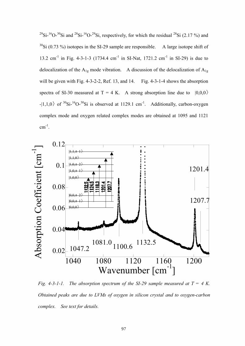
97
29Si-16O-30Si and 28Si-16O-29Si, respectively, for which the residual 28Si (2.17 %) and
30Si (0.73 %) isotopes in the SI-29 sample are responsible. A large isotope shift of
13.2 cm-1 in Fig. 4-3-1-3 (1734.4 cm-1 in SI-Nat, 1721.2 cm-1 in SI-29) is due to
delocalization of the A1g mode vibration. A discussion of the delocalization of A1g
will be given with Fig. 4-3-2-2, Ref. 13, and 14. Fig. 4-3-1-4 shows the absorption
spectra of SI-30 measured at T = 4 K. A strong absorption line due to |0,0,0〉
-|1,1,0〉 of 30Si-16O-30Si is observed at 1129.1 cm-1. Additionally, carbon-oxygen
complex mode and oxygen related complex modes are obtained at 1095 and 1121
cm-1.
Fig. 4-3-1-1. The absorption spectrum of the SI-29 sample measured at T = 4 K.
Obtained peaks are due to LVMs of oxygen in silicon crystal and to oxygen-carbon
complex. See text for details.
0.02
0.04
0.06
0.08
0.1
0.12
1040 1080 1120 1160 1200Abs
orpt
ion
Coe
ffic
ient
[cm
-1]
Wavenumber [cm-1]
1047.21081.0 1100.6 1132.5
1201.4
1207.7|0,0,0〉
|0,0,±1〉 |0,0,±2〉
|1,0,0〉
|1,0,±1〉
|1,0,±2〉
|1,1,0〉
|1,1,±1〉
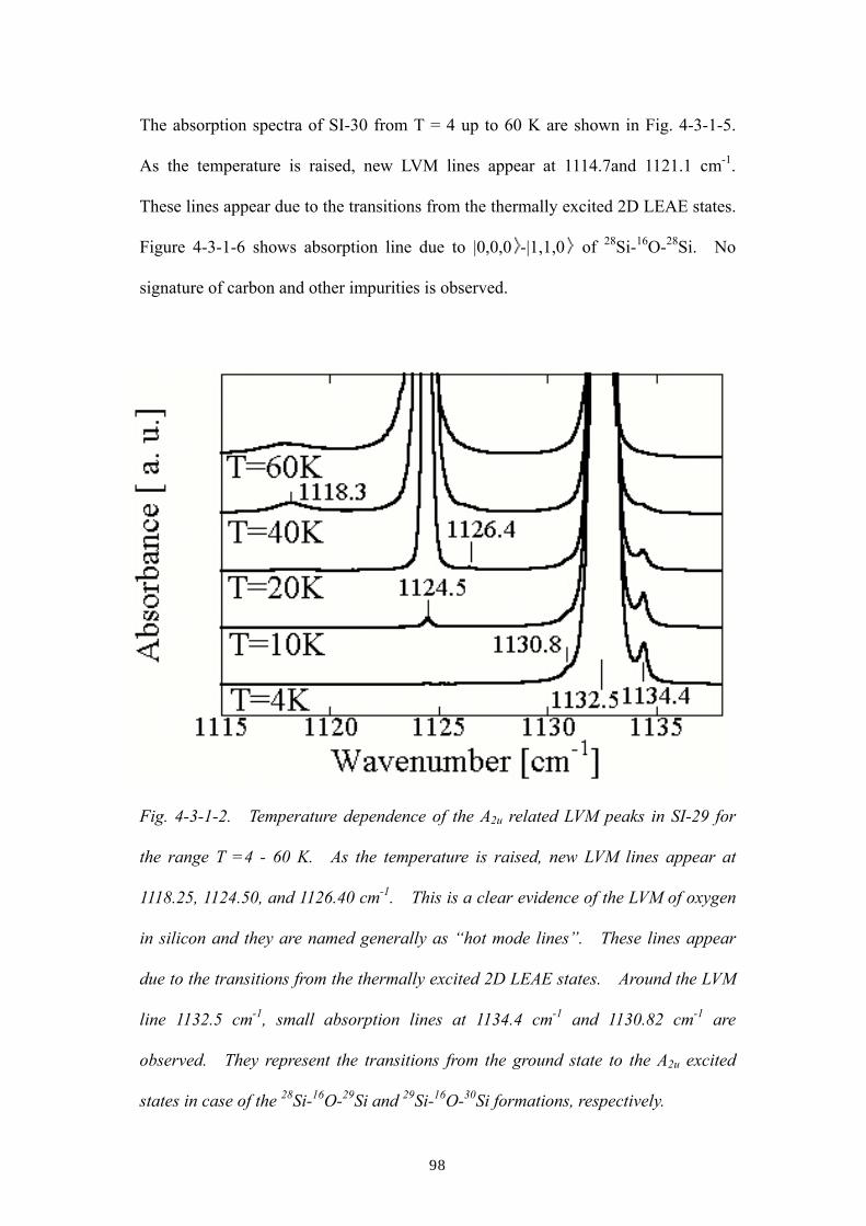
98
The absorption spectra of SI-30 from T = 4 up to 60 K are shown in Fig. 4-3-1-5.
As the temperature is raised, new LVM lines appear at 1114.7and 1121.1 cm-1.
These lines appear due to the transitions from the thermally excited 2D LEAE states.
Figure 4-3-1-6 shows absorption line due to |0,0,0〉-|1,1,0〉 of 28Si-16O-28Si. No
signature of carbon and other impurities is observed.
Fig. 4-3-1-2. Temperature dependence of the A2u related LVM peaks in SI-29 for
the range T =4 - 60 K. As the temperature is raised, new LVM lines appear at
1118.25, 1124.50, and 1126.40 cm-1. This is a clear evidence of the LVM of oxygen
in silicon and they are named generally as “hot mode lines”. These lines appear
due to the transitions from the thermally excited 2D LEAE states. Around the LVM
line 1132.5 cm-1, small absorption lines at 1134.4 cm-1 and 1130.82 cm-1 are
observed. They represent the transitions from the ground state to the A2u excited
states in case of the 28Si-16O-29Si and 29Si-16O-30Si formations, respectively.

99
The absorption lines observed in the previous reports and present studies are
summerized in Table 4-3-1-2.9-14 LVM frequencies described in the Italics in Table
4-3-1-2 are reported for the first time in this work.
1700 1710 1720 1730 1740 1750 17600.000
0.002
0.004
0.006
0.008
0.010
0.012
A
bsor
ptio
n C
oeff
icie
nt [c
m-1]
Wavenumber [cm-1]
Fig. 4-3-1-3. An absorption peak due to the transition from the ground state to A1g
+ A2u combined excited state in SI-29. A large isotope shift of 13.2 cm-1 (from
1734.4 cm-1 in SI-Nat and 1721.2 cm-1 in SI-30) is due to delocalization of A1g mode
vibration.

100
Fig. 4-3-1-4 The absorption spectra of the isotopically enriched 30Si crystal measured at
T = 4 K. A strong absorption line due to the A2u excited state of the 29Si-16O-29Si is
observed. Additionally, carbon-oxygen complex mode and oxygen related complex mode
are observed at 1095 and 1121 cm-1. The lines due to the 29Si-16O-30Si and 28Si-16O-30Si
were obtained at 1130.8 and 1132.5 cm-1, respectively.
LVM Calculated frequency
[cm-1]
Experimental data
[cm-1]
28Si-16O-28Si 1136.5 1136.5
28Si-16O-29Si 1134.1 1134.4
28Si-16O-30Si 1131.9 1132.0
29Si-16O-29Si 1131.7 1132.5
29Si-16O-30Si 1129.4 1130.8
29Si-16O-30Si 1127.0 1129.1
28Si-18O-28Si 1087.1 1084.4
29Si-18O-29Si 1079.8 1081.0
1100 1150 12000.10
0.15
0.20
0.25
0.30
C-O complex
A2u
30Si-16O-30Si
A2u
+ 2D LEAE30Si-16O-30Si
Abs
orpt
ion
Coe
ffic
ient
[cm-1]
Wave Number [cm-1]Wavenumber
Table 4-3-1-1 Comparison of the excitation frequencies of the |0,0,0 〉 - |1,1,0 〉
transition between experiments and calculation.
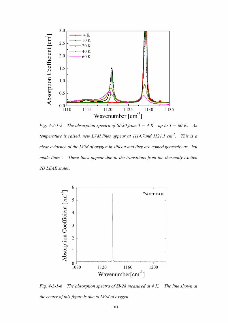
101
1110 1115 1120 1125 1130 11350.0
0.5
1.0
1.5
2.0
2.5
3.0 4 K 10 K 20 K 40 K 60 K 77 K
Abs
orpt
ion
Coef
ficie
nt [c
m-1]
Wavenumber [cm-1]Fig. 4-3-1-5 The absorption spectra of SI-30 from T = 4 K up to T = 60 K. As
temperature is raised, new LVM lines appear at 1114.7and 1121.1 cm-1. This is a
clear evidence of the LVM of oxygen in silicon and they are named generally as “hot
mode lines”. These lines appear due to the transitions from the thermally excited
2D LEAE states.
0
1
2
3
4
5
6
1080 1120 1160 1200
28Si at T = 4 K
Abs
orpt
ion
Coe
ffic
ient
[cm
-1]
Wavenumber[cm-1]
Fig. 4-3-1-6 The absorption spectra of SI-28 measured at 4 K. The line shown at
the center of this figure is due to LVM of oxygen.
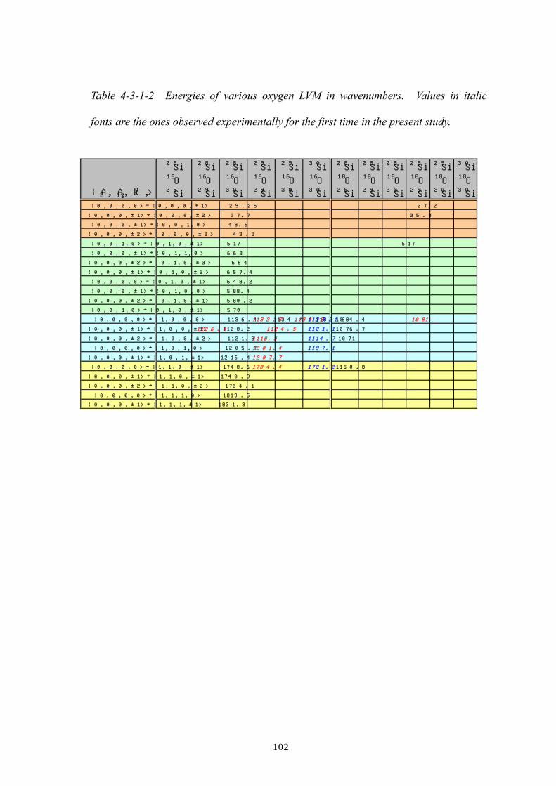
102
Table 4-3-1-2 Energies of various oxygen LVM in wavenumbers. Values in italic
fonts are the ones observed experimentally for the first time in the present study.
28Si
28Si
28Si
29Si
29Si
30Si
28Si
28Si
28Si
29Si
29Si
30Si
16O
16O
16O
16O
16O
16O
18O
18O
18O
18O
18O
18O
28Si
29Si
30Si
29Si
30Si
30Si
28Si
29Si
30Si
29Si
30Si
30Si
¦0,0,0,0>→¦0,0,0,±1> 29.25 27.2
¦0,0,0,±1>→¦0,0,0,±2> 37.7 35.3
¦0,0,0,±1>→¦0,0,1,0> 48.6
¦0,0,0,±2>→¦0,0,0,±3> 43.3
¦0,0,1,0>→¦0,1,0,±1> 517 517
¦0,0,0,±1>→¦0,1,1,0> 668
¦0,0,0,±2>→¦0,1,0,±3> 664
¦0,0,0,±1>→¦0,1,0,±2> 657.4
¦0,0,0,0>→¦0,1,0,±1> 648.2
¦0,0,0,±1>→¦0,1,0,0> 588.4
¦0,0,0,±2>→¦0,1,0,±1> 580.2
¦0,0,1,0>→¦0,1,0,±1> 570
¦0,0,0,0>→¦1,0,0,0> 1136.4 1134.4 1132.6 1132.5 1130.8 1129.1 1084.4 1081
¦0,0,0,±1>→¦1,0,0,±1> 1128.2 1126.4 1124.5 1121.1 1076.7
¦0,0,0,±2>→¦1,0,0,±2> 1121.9 1118.3 1114.7 1071
¦0,0,0,0>→¦1,0,1,0> 1205.7 1201.4 1197.1
¦0,0,0,±1>→¦1,0,1,±1> 1216.4 1207.7
¦0,0,0,0>→¦1,1,0,±1> 1748.6 1734.4 1721.2 1150.8
¦0,0,0,±1>→¦1,1,0,±1> 1740.9
¦0,0,0,±2>→¦1,1,0,±2> 1734.1
¦0,0,0,0>→¦1,1,1,0> 1819.5
¦0,0,0,±1>→¦1,1,1,±1> 1831.3
¦A2u,A1g,k,l >

103
4.3.2. Effect of the 2nd nearest and beyond nearest-neighboring host atoms
We shall now evaluate the effect of the second and beyond nearest Si neighbors
by focusing on a particular configuration 28Si-16O-29Si and compare the frequencies
of the A2u mode between the SI-29 and SI-Nat samples. Figure 4-3-2-1 shows the
absorption peaks of the |0,0,0〉-|1,0,0〉 excitations of the 28Si-16O-29Si in SI-29 and
SI-Nat, which shows the peak frequency shift of 0.07 cm-1. This small but obvious
shift is caused by the isotope effect of the second and beyond nearest neighboring Si
atoms, since those in SI-29 are mostly 29Si while those in SI-Nat are mostly 28Si
isotopes. Calculations based on the linear chain model described in chapter 4.3.1
predict the shift of approximately 0.03 cm-1 (see Fig.4-3-2-3). Although there is a
factor between the experiment and calculation, we believe this agreement within the
same order of magnitude shows unambiguously the effect of second and beyond
nearest Si neighbors. Figure 4-3-2-2 shows the amplitude of the displacement of
each atom in our linear-chain calculation. For the case of A2u, the second nearest
neighbor Si is displaced clearly, i.e., isotope substitution of the second neighbors
should shift the LVM frequency. Although much larger effect of the second and
beyond nearest neighbors is expected for A1g as seen in Fig. 4-3-2-2, we could not
observe A1g related absorption lines experimentally due to the insufficient thickness
(<1mm) of our sample. Our discussion here suggests that the origin of large
isotope shifts of the A1g mode and the A1g + A2u combined mode discussed in Ref.
14 and 22 may be due to the second and beyond nearest neighbors. In order to
observe the effect of the second and beyond nearest neighbors on impurity LVMs,
one has to select carefully the mass of the localized impurity and host
semiconductors. For example, a hydrogen atom is so much lighter than the host Si
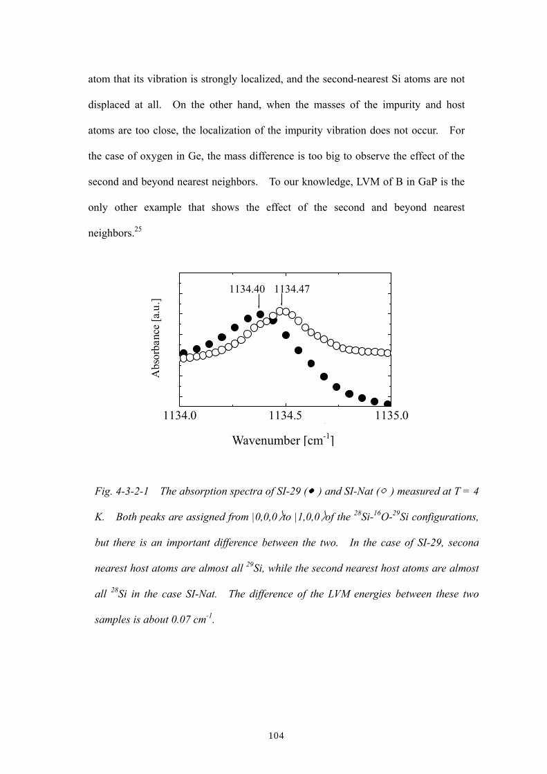
104
atom that its vibration is strongly localized, and the second-nearest Si atoms are not
displaced at all. On the other hand, when the masses of the impurity and host
atoms are too close, the localization of the impurity vibration does not occur. For
the case of oxygen in Ge, the mass difference is too big to observe the effect of the
second and beyond nearest neighbors. To our knowledge, LVM of B in GaP is the
only other example that shows the effect of the second and beyond nearest
neighbors.25
Fig. 4-3-2-1 The absorption spectra of SI-29 () and SI-Nat () measured at T = 4
K. Both peaks are assigned from |0,0,0〉to |1,0,0〉of the 28Si-16O-29Si configurations,
but there is an important difference between the two. In the case of SI-29, second
nearest host atoms are almost all 29Si, while the second nearest host atoms are almost
all 28Si in the case SI-Nat. The difference of the LVM energies between these two
samples is about 0.07 cm-1.
1134.0 1134.5 1135.0
1134.471134.40
Abs
orba
nce
[a.u
.]
Wave Number [cm-1] Wavenumber [cm-1]

105
Fig. 4-3-2-2 The calculated displacement patterns of the A2u and A1g modes by a
linear chain model. The horizontal axis means the position of oxygen and silicon
atoms. The vertical axis means the intensities of the vibrations of the atoms.
Oxygen atom is positioned at the center of this linear chain. In this particular
calculation, the Si atom on the left of oxygen is 28Si. Other silicon atoms are 29Si.
Fig. 4-3-2-3 The calculational results of the energy shifts of 28Si-16O-29Si
configuration due to the second and beyond nearest silicon atoms as a function of
the number of atoms in a calculational cell. The calculational cell is
composed 99 atoms which is confirmed large enough to calculate the energy
shift. The big energy shift in the case of A1g mode is consistent with the weaker
localization of A1g mode than that of A2u mode.
20 40 60 80 1000.0
0.5
1.0
1.5
2.0
2.5
A2u: 0.03 cm-1
A1g: 2.5 cm-1
Ene
rgy
Shif
t [cm-1
]
The Number of Atoms
A2u mode
A1g mode
Inte
nsity
[a. u
.]
Position
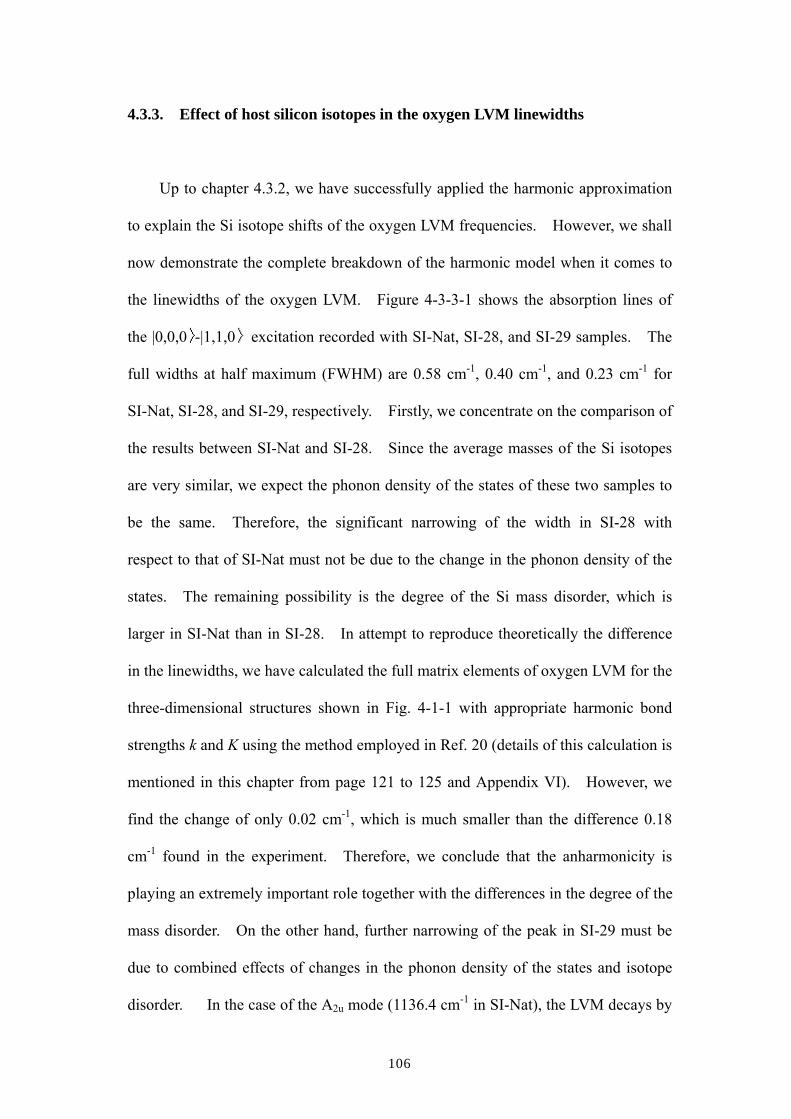
106
4.3.3. Effect of host silicon isotopes in the oxygen LVM linewidths
Up to chapter 4.3.2, we have successfully applied the harmonic approximation
to explain the Si isotope shifts of the oxygen LVM frequencies. However, we shall
now demonstrate the complete breakdown of the harmonic model when it comes to
the linewidths of the oxygen LVM. Figure 4-3-3-1 shows the absorption lines of
the |0,0,0〉-|1,1,0〉 excitation recorded with SI-Nat, SI-28, and SI-29 samples. The
full widths at half maximum (FWHM) are 0.58 cm-1, 0.40 cm-1, and 0.23 cm-1 for
SI-Nat, SI-28, and SI-29, respectively. Firstly, we concentrate on the comparison of
the results between SI-Nat and SI-28. Since the average masses of the Si isotopes
are very similar, we expect the phonon density of the states of these two samples to
be the same. Therefore, the significant narrowing of the width in SI-28 with
respect to that of SI-Nat must not be due to the change in the phonon density of the
states. The remaining possibility is the degree of the Si mass disorder, which is
larger in SI-Nat than in SI-28. In attempt to reproduce theoretically the difference
in the linewidths, we have calculated the full matrix elements of oxygen LVM for the
three-dimensional structures shown in Fig. 4-1-1 with appropriate harmonic bond
strengths k and K using the method employed in Ref. 20 (details of this calculation is
mentioned in this chapter from page 121 to 125 and Appendix VI). However, we
find the change of only 0.02 cm-1, which is much smaller than the difference 0.18
cm-1 found in the experiment. Therefore, we conclude that the anharmonicity is
playing an extremely important role together with the differences in the degree of the
mass disorder. On the other hand, further narrowing of the peak in SI-29 must be
due to combined effects of changes in the phonon density of the states and isotope
disorder. In the case of the A2u mode (1136.4 cm-1 in SI-Nat), the LVM decays by

107
at least three phonons since the maximum of the Si phonon frequency is 524.5 cm-1.
One possibility is the change in three-phonon density of states at the LVM
frequencies between the peak positions 1132.5 cm-1 in SI-29, and 1136.4 cm-1 in
SI-28 and SI-Nat. FWHM=0.23 cm-1 in SI-29 is 0.35 cm-1 smaller than
FWHM=0.58 cm-1 in SI-Nat, in part because of the smaller phonon density of the
states at 1132.5 cm-1 than that at 1136.4 cm-1 leading to slower decay of oxygen
vibrations, and in part because of less Si mass disorder in the 97.10% isotopically
enriched SI-29 sample leading to less inhomogeneous broadening of the peak.
0.40 cm-1
0.58 cm-1
SI-29
SI-28
SI-Nat
0.23 cm-1
1132 1134 1136 1138
T=4K
Wavenumber [cm-1]
Abs
orba
nce
[a.u
.]
Fig. 4-3-3-1. A comparison of the width of the LVM lines of |0,0,0〉- |1,1,0〉transitions
in SI-29, SI-28, and SI-Nat.

108
It suggests that further enrichment of 29Si isotopes towards 100% will sharpen the
line beyond 0.23 cm-1 because of the surprisingly large contribution of the isotopic
mass disorder to the width of the oxygen A2u mode in Si.

109
References
1 E. E. Haller, J.Appl. Phys, 77, 2857 (1995).
2 F. Widulle, T. Ruf, M Konuma, I. Silier, M. Cardona, W. Kriegseis and V. I.
Ozhogin, Solid State Commun. 118, 1 (2001).
3 T. Ruf, R. W. Henn, M. Asen-Palmer, E. Gmelin, M. Cardona, H. -J. Pohl, G. G.
Devyatych and P. G. Sennikov, Solid State Commun. 115, 243 (2000).
4 D. Karaiskaj, M. L. W. Thewalt, T. Ruf, M. Cardona, H. –J. Pohl, G. G.
Deviatych, P. G. Sennikov, and H. Riemann, Phys. Rev. Lett. 86, 6010 (2001).
5 D. Karaiskaj, M. L. W. Thewalt, T. Ruf, M. Cardona, and M. Konuma, Phys. Rev.
Lett. 89, 016401 (2002).
6 Ken–ichiro Takyu, Kohei M. Itoh, Kunihiko Oka, Naoaki Saito and Valerii I.
Ozhogin, Jpn. J. Appl. Phys. 38, 1493 (1999).
7 A. D. Bulanov, G. G. Devyatych, A. V. Gusev, P. G. Sennikov, H. –J. Pohl, H.
Riemann, H. Schilling, and P. Becker, Cryst. Res. Technol. 35, 1023 (2000).
8 Hyunjung Kim, R. Vogelgesang, A. K. Ramdas, and S. Rodriguez, M. Grimsditch,
and T. R. Anthony, Phys. Rev. B 57, 15315 (1998).
9 R. C. Newman, J. Phys. Condens. Matter 12, 335 (2000).
10 D. R. Bosomworth, W. Hayes, A. R. Spray, and G. D. Watkins, Proc. Roy. Soc.
Lond. A. 317, 133 (1969).
11 H. J. Hrostowski and R. H. Kaiser, Phys. Rev. 107, 966 (1957).
12 H. J. Hrostowski and B. J. Alder, J. Chem. Phys. 33, 980 (1960).
13 Hiroshi Yamada-Kaneta, Physica B 302-303, 172 (2001).
14 B.Pajot, E. Artacho, C. A. Ammerlaan, and J-M. Spaeth, J. Phys. Condens.
Matter 7, 7077 (1995).
110
15 R. Jones, A. Umerski, and S.Öberb, Phys. Rev. B 45, 11321 (1992).
16 M. D. McCluskey, J.Appl. Phys, 87, 3593 (2000).
17 B. Sun, A. Fraser, and G. Lüpke, private communication.
18 A. J. Mayur, M. Dean Sciacca, M. K. Udo, A. K. Ramdas, K. Itoh, J. Wolk, and
E. E. Haller, Phys. Rev. B 49, 16293 (1994).
19 E. Artacho, F. Yndurain, B. Pajot, R. Ramirez, C. P. Herrero, L. I. Khirunenko,
K. M. Itoh, E. E. Haller, Phys. Rev. B 56, 3820 (1997).
20 Hiroshi Yamada-Kaneta, Chioko Kaneta, and Tsutomu Ogawa, Phys. Rev. B 42,
9650 (1990).
21 Hiroshi Yamada-Kaneta, Chioko Kaneta, and Tsutomu Ogawa, Phys. Rev. B 47,
9338 (1993).
22 H. Yamada-Kaneta, Phys. Rev. B 58, 7002 (1998).
23 G. Davies and R. C. Newman, in Handbook on Semiconductors Completely
Revised Edition (Elsevier Science Publishers B. V., Amsterdam, 1992), vol. 3,
Chapter 21, (1994).
24 S. P. Chappell, M. Claybourn, R. C. Newman, K. G. Barraclough, Semicon. Sci.
Technol. vol. 3, no. 10, 1047 (1988).
25 D. A. Robbie, M. J. L. Sangster, E. G. Grosche, R. C. Newman, T. Pletl, P.
Pavone, and D. Strauch, Phys. Rev. B 53, 9863 (1996).
26 Jiro Kato, Kohei M. Itoh, Hiroshi Yamada-Kaneta, and Hans-Joachim Pohl,
Proceedings of the 26th International Conference on the Physics of
Semiconductors, Edinburgh, July 29-August 2, 2002, Institute of Physics
Publishing, in press.

111
Chapter 5: Summary and future prospects
In this thesis we have discussed the effect of electronic correlation and isotopic
mass disorder on impurity infrared absorption spectra, especially on the linewidths.
In chapter 3, we have discussed the broadening of ground-state to bound
excited-state transitions of shallow donors in strongly compensated n-type
Ge:(As,Ga) in the presence of electric fields and their gradients, arising from
randomly distributed ionized impurities. Quantitative comparison of the
experimentally obtained linewidths with Monte Carlo simulation results made
possible a unique determination of the ionized impurity distribution in the samples.
A clear evidences for the random-to-correlated transition of the ionized impurity
distribution as a function of the ionized impurity concentration and of temperature
was presented.
In chapter 4, we have discussed a high-resolution infrared absorption study of
the localized vibrational modes (LVMs) of oxygen in isotopically enriched 28Si and
29Si single crystals. Isotope shifts of LVM frequencies from those in natural Si
were clearly observed not only due to the change of the average mass in the nearest
neighbor silicon atoms but also to that of the second and beyond nearest neighbors.
The amount of these shifts agrees quantitatively with calculations based on the
harmonic approximation. However, the linewidths of certain LVMs in the enriched
samples were much narrower than those in natural Si, despite the fact that the
harmonic approximation predicts very little dependence of the width on the host Si
isotopic composition. Such observation suggested that both anharmonicity and
inhomogeneous broadening due to isotopic disorder are playing important roles for
the determination of the oxygen LVM linewidths.
112
In this thesis, a strong focus was placed on the linewidth of the absorption
peaks. Understanding of the linewidths provides the bases for determination of
impurity concentrations and crystalline quality because the linewidth is very
sensitive not only to the impurity concentration but also to the quality of crystals.
Electric field, defects, stress, and other extrinsic properties affect the linewidth
significantly. Once high crystalline quality is confirmed, it is possible to use the
absorption spectroscopy to determine the concentrations of the electrically active
majority and minority impurity concentrations, and those of electrically inactive
localized impurities. In order to precisely determine these concentrations, it is
necessary to understand the physics of line broadening. In this regard, the results of
this thesis may be proven important for the characterization of semiconductors, i.e.,
technology, in the future.
Future prospectives includes further understanding of the linewidth. For
the work presented in chapter 3, open questions include the development of the
quantitative theoretical models describing the ionized impurity concentration and
temperature induced transition between correlated and random transition. Such
understanding is also of technological importance because determination of the
impurity concentration based on the linewidth depends on the temperature of the
measurement. For example, if the measurement is performed at T=4 K, one needs
to know what linewidths we expect for both random and partially correlated
distributions of impurities. In this thesis we have probed the linewidth only for the
compensation K<0.7. It is of interest in the future to probe the region K>0.7.
What happens when two kinds of donors and one kind of acceptor are contained was
not discussed in this thesis. Two kinds of donors have different energy states and,
with appropriate choices of compensation, a situation can be realized in which the

113
shallower donors are partially ionized while deeper donors are not ionized at all. In
this case we expect to observe correlated distribution only for the shallower donors.
The linewidth of the deeper donors should correspond to that of random distribution.
This kind of observation will further confirm the findings in chapter 3.
Physics of oxygen localized vibrational modes has been proven very rich in
chapter 4. It represents the chemical bonding between oxygen and silicon which
can not be described by the simple harmonic approximation. Unexpectedly large
isotope effects of host Si isotopes have been found. There is no doubt for the
importance of the investigation with silicon whose isotopic composition is
systematically modified. For example a crystal with 1:1 mixture of 28Si and 30Si
has a maximum Si disorder and its effect on the linewidth is of significant interest.
Also measurement and discussion of low frequency modes such as 2D LEAE as a
function of Si isotopic composition will provide better understanding of physics of
oxygen LVM in Si. The effect of multi-phonon emission is also important to
understand the LVM linewidth. We must calculate the multi-phonon density of
states to consider the effect quantitatively in the future.

114
Appendixes
Appendix A: Theoretical models for linewidth calculation in Chapter 3
A.1. Importance of using an anisotropic wavefunction
Larsen1 has calculated the width of the absorption peak of donors in GaAs by
using Eq. (25) in Ref. 1, i.e.,
⋅−+±
∂∂
−⋅⋅⋅=∆ 23 3*22*3* 156186 εaNTTz
ERyaNE IBAz
I . (A-1-1)
Eq. (A-1-1) represents the perturbation energy of the electron bound to the 2p±
orbital of shallow donors assuming a completely isotropic conduction band. A
distribution in perturbation energies for an ensemble of donor electrons leads to a
broadening of the peak. The circumstance of our experiment is very similar to that
in Ref. 1 in chapter 3 except for the point that our material (Ge:As) has the strong
anisotropy in the conduction bands. As a first-order approximation, Eq. (A-1-1)
can be employed to simulate our experimental results. However, applicability of
Eq. (A-1-1) for quantitative analysis remains questionable due to the strong
anisotropy (the longitudinal effective mass is approximately 20 times larger than the
transverse effective mass) of Ge conduction bands. Therefore, a donor electron
wavefunction for Ge should be composed based on a sum of eight wavefunctions
whose longitudinal axes (hereafter z axes) correspond to the directions of [ ]111 ,
[ ]111 , [ ]111 , [ ]111 , [ ]111 , [ ]111 , [ ]111 , and [ ]111 . The wavefunction of

115
our interest, ( )±p2ψ , is composed of the strong anisotropic wavefunctions and their
Bloch wavefunctions ( )±pi 2ϕ as follows,
( ) ( )∑ ±± ⋅=4
22i
ii pcp ϕψ , (A-1-2)
where ∑ =4
2 1i
ic . ( )±p2ψ is expressed as E+T1+T2 using the standard notations
of group theory in Td symmetry. Thus it is important for us to take into account the
anisotropy since there is no isotropic notation such as A1 in the ( )±p2ψ orbital.
In order to estimate the perturbation energy E∆ for the case of the Ge
anisotropic ( )±p2ψ wavefunction, we use:
( )
⋅+±−
∂∂
⋅⋅⋅=∆ ±±
±±± 1,1,222
22
1,1,222
1,1,222
1,1,2** cos
31
433
21 ψθψψψ ϕi
BAz
I eLrTTrzz
ERyaNE
(A-1-3)
where IN is ionized impurity concentration, *a is effective Bohr radius, and *Ry
is effective Rydberg constant. z
Ez
∂∂ and 22
BA TT + are given by
( )∑ −−=∂∂ 22
50
3 jjj
jz RZRe
zE
ε and (A-1-4)
( ) ( )2
50
2
225
0
22 2
⋅+
−=+ ∑∑ jj
j
jjj
j
jBA YX
Re
YXRe
TTεε
, (A-1-5)
respectively. The wavefunction for the 2p± orbital ( 1,1,2 ±ψ ) is given by:

116
*25*
111,21,1,2 sin
8
1 ar
i erea
YR−
±±± ⋅⋅=⋅= θ
πψ ϕ , (A-1-6)
where 1,2R and 11±Y are the radial wavefunction and the spherical harmonic
wavefunction, respectively. The direction of z-axis corresponds to the longitudinal
axis of a wavefunction. We ignored quadratic Stark effect in Eq. (A-1-3) since this
contribution is believed to be negligibly small for our set of samples.
In our calculation z
Ez
∂∂ and 22
BA TT + are quantitatively obtained by
numerical calculation based on the Monte Carlo method. Then the perturbation
energy E∆ is obtained directly from Eq. (A-1-3) since values for *a , *Ry , and
IN are known.
We shall describe in the following two sections how we obtain the anisotropic
wavefunctions based on Eq. (A-1-6) using well-established methods developed by
Kohn-Luttinger2 and by Faulkner3 We shall compare the three values of E∆
obtained by;
i) isotropic wavefunction [Eq. (A-1-1)],
ii) anisotropic wavefunction of Kohn-Luttinger, and
iii) anisotropic wavefunction of Faulkner
directly at the end of this chapter.
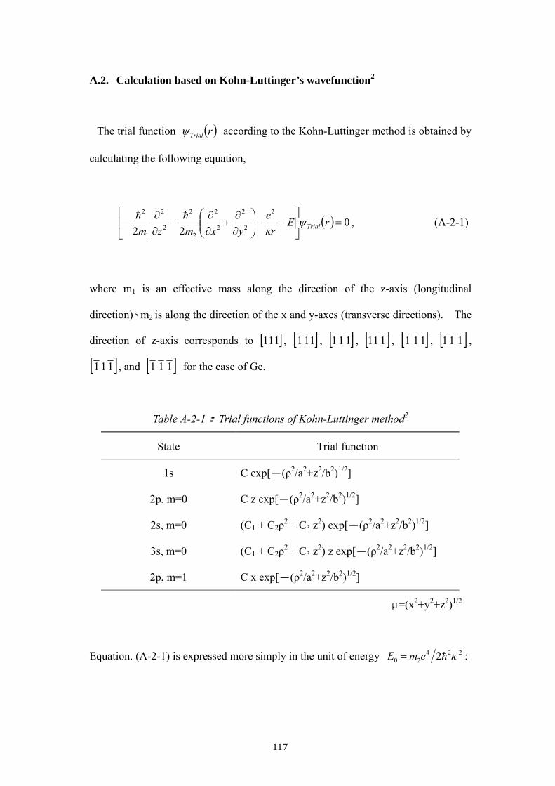
117
A.2. Calculation based on Kohn-Luttinger’s wavefunction2
The trial function ( )rTrialψ according to the Kohn-Luttinger method is obtained by
calculating the following equation,
( ) 022
2
2
2
2
2
2
2
2
2
1
2
=
−−
∂∂
+∂∂
−∂∂
− rEr
eyxmzm Trialψ
κhh , (A-2-1)
where m1 is an effective mass along the direction of the z-axis (longitudinal
direction)、m2 is along the direction of the x and y-axes (transverse directions). The
direction of z-axis corresponds to [ ]111 , [ ]111 , [ ]111 , [ ]111 , [ ]111 , [ ]111 ,
[ ]111 , and [ ]111 for the case of Ge.
Table A-2-1: Trial functions of Kohn-Luttinger method2
State Trial function
1s C exp[-(ρ2/a2+z2/b2)1/2]
2p, m=0 C z exp[-(ρ2/a2+z2/b2)1/2]
2s, m=0 (C1 + C2ρ2 + C3 z2) exp[-(ρ2/a2+z2/b2)1/2]
3s, m=0 (C1 + C2ρ2 + C3 z2) z exp[-(ρ2/a2+z2/b2)1/2]
2p, m=1 C x exp[-(ρ2/a2+z2/b2)1/2]
ρ=(x2+y2+z2)1/2
Equation. (A-2-1) is expressed more simply in the unit of energy 22420 2 κhemE = :

118
( ) 022
2
2
2
2
2
=
−−
∂∂
+∂∂
+∂∂
− rEryxz Trialψγ , (A-2-2)
where 22
2 emaB κh= is the effective Bohr radius and 12 mm=γ is a ratio of
effective masses. A trial function for the 1s orbital is expressed by
( ) 2
2
2
2
2_1_1 b
za
orbitalsTrial eba
r+−
=ρ
πψ , (A-2-3)
and the energy of 1s orbital orbitalsE _1 is given by
( ) ( )rHrE orbitalsTrialorbitalsTrialorbitals _1__1_*
_1 ψψ=
dxdydzebaryxz
eba
bz
abz
a∫∫∫+−+−
−
∂∂
+∂∂
+∂∂
−
=
2
2
2
2
2
2
2
2
22
2
2
2
2
2*
2
121 ρρ
πγ
π.
(A-2-4)
orbitalsE _1 is numerically obtained by the lowering the energy through parameters a
and b in Eq. (A-2-4). Before we perform the calculation for Ge, we have checked
the reliability of our calculation using Si ( 2079.0=γ ) as an example. For the 1s
orbital of Si, we have obtained the minimum energy orbitalsE _1 =-1.56524 with
a=0.74426 and b=0.430841. With the relative dielectric constant of Si 12=κ , we
obtain -0.029eV for E1s orbital, which is in complete agreement with the original
calculation of Kohn and Luttinger in Ref. 2. In the same manner, the minimum
energies have been calculated as a function of γ (see Fig. A-2-1). The program
code of calculation for Ge ( 05134.0=γ ) is written in Appendix B.

119
We calculate the energy shift for the case of 2p(m=1) orbital as the same way for the
case of 1s orbital. The wavefunction is
( ) 2
2
2
2
4_)1(2_bz
aorbitalmpTrial e
baxr
+−
= =ρ
πψ . (A-2-5)
The minimum energy 36622.0_)1(2 −== orbitalmpE for Ge ( 0534.0=γ ) has been
obtained with a=1.53483、b=0.619206. The minimum energy orbitalmpE _)1(2 = as a
function of γ is shown in Fig. A-2-2.
-2.5
-2
-1.5
-1
-0.5
0.2 0.4 0.6 0.8 1
Ener
gy [/
E 0]
γ1/3
Fig. A-2-1 The energy of 1s orbital (m=0) vs. γ 1/3 according to the Kohn-Luttinger
method.
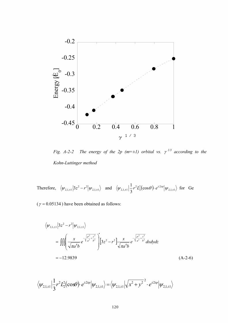
120
Therefore, 1,1,222
1,1,2 3 ±± − ψψ rz and ( ) 1,1,222
22
1,1,2 cos31
±±
± ⋅ ψθψ ϕieLr for Ge
( 05134.0=γ ) have been obtained as follows:
1,1,222
1,1,2 3 ±± − ψψ rz
[ ] dxdydzeba
xrzeba
x bz
abz
a∫∫∫+−+−
−
=
2
2
2
2
2
2
2
2
4
22
*
43
ρρ
ππ
9839.12−= (A-2-6)
( ) 1,1,22
222
1,1,21,1,222
22
1,1,2 cos31
±±
±±±
± ⋅+=⋅ ψψψθψ ϕϕ ii eyxeLr
-0.45
-0.4
-0.35
-0.3
-0.25
-0.2
0 0.2 0.4 0.6 0.8 1
Ener
gy [E
0]
γ1/3
Fig. A-2-2 The energy of the 2p (m=±1) orbital vs. γ 1/3 according to the
Kohn-Luttinger method

121
[ ] dxdydzeba
xyxeba
x bz
abz
a∫∫∫+−+−
+
=
2
2
2
2
2
2
2
2
4
22
*
4
ρρ
ππ
1341.14= (A-2-7)
The program code of the calculation is written in Appendix C.
Finally, we shall incorporate an appropriate effective mass m* and the ionized
impurity concentration NI to obtain realistic values for the energy shift of the 2p±
state for Ge as the following:
( )
⋅+±−
∂∂
⋅⋅⋅=∆ ±±
±±± 1,1,222
22
1,1,222
1,1,222
1,1,2** cos
31
433
21 ψθψψψ ϕi
BAz
I eLrTTrzz
ERyaNE
( )
×+±−×
∂∂
⋅⋅⋅=2*222*** 1341.14
439839.12
21 aTTa
zERyaN BA
zI
+±
∂∂
−⋅⋅⋅= 22*3* 6006.104920.6 BAz
I TTz
ERyaN . (A-2-8)
122
A.3. Calculation based on Faulkner’s wavefunction3
An anisotropic trial function mln ,,ψ is expressed as follows according to Faulkner’s
method
( ) ( ) ( )φθαγβφθϕ
γβψ ,,,, ,
41
,,
41
,,l
mlnmlnmln YrRr ⋅
=
= , (A-3-1)
where α and β are parameters. The normalized radial wavefunctions are:
( ) ( )( )[ ]
( )nrLen
rln
lnn
rR lln
nrl
ln αααα α 22!
!12, 121
21
32
23
,+
−−−×
+−−
= . (A-3-2)
2
22
++= zyxr
γβ
(A-3-3)
where ( )zL kp is the Laguerre polynomial:
( ) ( ) ( )[ ]( ) ( )
sskp z
sskspkpzL
!!!!1
2
+−+
−=∑ (A-3-4)
and ( )φθ ,lmY is a function of the Spherical harmonics. The Hamiltonian matrix is
expressed as:
nlmHmln ′′′
dxdydzzyxrzyx
zyx mlnmln
−
∂∂
+∂∂
+∂∂
−
= ′′′′′′∫∫∫ γ
βψγγβψ
γβ ,,2,, ,,2
2
2
2
2
2*
,,

123
( ) ( )( )
++−
∂∂
−−
∂∂
+∂∂
+∂∂
−= ′′′∫∫∫ 2222
2
2
2
2
2
2
2*
,,21,,
zyxzzyxzyxmln
βγβψ
γβ
( )dxdydzzyxmln ,,,,ψ× .
(A-3-5)
For the case of ll =′ , the energy is expressed as:
( ) ( ) ( ) ( ) ( )( )( )
+−
−++−−+′−=′′′
32126121
3111,;,,2,,,,
21
llmlllnlnJllImlnHmln β
( ) ( ) ( ) mmnn lnlnJln
l′′
′+−× δααδ ,;,2 )1(
2
2
, . (A-3-6)
For the case of 2−=′ ll is given by:
( ) ( ) ( ) mmlnlnJllImlnHmln ′−′−−=′′′ δ,;2,,22,,,, 1
( ) ( )( )( )[ ]
( )( )( ) ( ) ( )( )lnlnJ
nl
nl
llmlml
lmm ,;2,2
21
32121
121 2
2
2
2
2212222
−′
′−
+×
−+−−−
−−+ ′ ααδβ
( ) ( )[ ] ( )( ) ( ) ( )( ) ( ),;2,,;2,12,;2,2 01 lnlnDlnlnJlllnlnJll −′+−′−+−′−+− αα .(A-3-7)
For the case of 1,0;2 ≠±=′ jjll is given by:
( ) ( ) ( ) mmlnlnJllImlnHmln ′′′′−=′′′ δ,;,,2,,,, 1 , (A-3-8)
where

124
( ) ( ) ( )( )
Ω−−
ΩΩ=′ ∫
′
dYYllIl
ml
m
θβγ 2
*
cos11, (A-3-9)
( )( ) ( )( ) ( )( )drrlRrlRlnlnJ lnln ,,,;, ,0 ,0 αα∫
∞
′′ ′=′′ (A-3-10)
( )( ) ( )( ) ( )( )drrlRrlrRlnlnJ lnln ,,,;, ,0 ,1 αα∫
∞
′′ ′=′′ (A-3-11)
( )( ) ( )( ) ( )( )drrlRrlRrlnlnJ lnln ,,,;, ,0 ,22 αα∫
∞
′′ ′=′′ (A-3-12)
( )( ) ( )( ) ( )( )drrlRr
rrlRlnlnJ lnln ,,,;, ,0 ,3 αα∫
∞
′′ ∂∂′=′′ . (A-3-13)
We shall obtain wavefunctions in terms of eigenfunctions composed of energies
Eq. (A-3-6), (A-3-7), and (A-3-8). It can be achieved by minimization of the sum
of the eigenvalues. The following matrix is used to obtain the wavefunctions of
7,6,5,4,3,2,1,1 =±== nml :
±±±±±±±±
±±±±±±±±±±
1,1,71,1,71,1,61,1,71,1,21,1,71,1,71,1,6
1,1,21,1,31,1,21,1,31,1,71,1,21,1,31,1,21,1,21,1,2
HHHH
HHHHH
L
OMM
ML
L
.
Results of our calculation are shown in Table 3-2-3-1. Also, Fig. 3-2-3-2 shows
the γ dependency of 1,1,222
1,1,2 3 ±± − ψψ rz and ( ) 1,1,222
22
1,1,2 cos31
±±
± ⋅ ψθψ ϕieLr
in Eq. (A-1-3), for the case of the 2p± orbital.
From the results of Fig. A-3-2, we obtain for the case of Ge ( 05134.0=γ ),

125
γ 2p± 3p± 4p± 5p± 6p± 7p± α(1) α(3) β
0.001 -0.421482 -0.18733 -0.10537 -0.06744 -0.04683 -0.03441 1.44575 0.5002 0.0552
0.01 -0.399424 -0.17752 -0.09986 -0.06391 -0.04438 -0.03261 1.38524 0.5920 0.1564
0.05134 -0.365698 -0.16253 -0.09142 -0.05851 -0.04063 -0.02985 1.3014 0.7720 0.3134
0.1 -0.34654 -0.15402 -0.08663 -0.05545 -0.0385 -0.02829 1.25229 0.8123 0.4073
0.2079 -0.320453 -0.14242 -0.08011 -0.05127 -0.03561 -0.02616 1.18433 0.8499 0.5499
0.5 -0.28328 -0.1259 -0.07082 -0.04532 -0.03148 -0.02312 1.08709 0.9112 0.7710
0.8 -0.260895 -0.11595 -0.06522 -0.04174 -0.02899 -0.0213 1.03074 0.9910 0.9295
1.0 -0.249929 -0.11108 -0.06248 -0.03999 -0.02777 -0.0204 0.996037 1.0021 1.009
A unit of energy is 22420 2/ κε hem= .
-0.5
-0.4
-0.3
-0.2
-0.1
0
0 0.2 0.4 0.6 0.8 1
2p±
3p±
4p±
5p±
6p±
7p±
Ener
gy [/
E 0]
γ1/3
Table A-3-1: The energies of the impurity levels obtained from the Faulkner’s method.
Fig. A-3-1: The energy of the impurity levels obtained by Faulkner’s method.

126
*1,1,2
221,1,2 9638.123 arz −=− ±± ψψ , (A-3-14)
( ) *1,1,2
222
21,1,2 1181.14cos
31 aeLr i =⋅ ±
±± ψθψ ϕ . (A-3-15)
The program code of this calculation is written in Appendix D.
As a result, the energy shift of the 2p± orbital due to the electric field is given by:
( )
⋅+±−
∂∂
⋅⋅⋅=∆ ±±
±±± 1,1,222
22
1,1,222
1,1,222
1,1,2** cos
31
433
21 ψθψψψ ϕi
BAz
I eLrTTrzz
ERyaNE
( )
×+±−×
∂∂
⋅⋅⋅=2*222*** 1181.14
430638.12
21 aTTa
zERyaN BA
zI
+±
∂∂
−⋅⋅⋅= 22*3* 5886.100319.6 BAz
I TTz
ERyaN (A-3-16)
-20
-10
0
10
20
30
0 0.2 0.4 0.6 0.8 1 1.2
(1)(2)
Ener
gy[/E
0]]
γ1/3
Fig. A-3-2 1,1,222
1,1,2 3 ±± − ψψ rz and ( ) 1,1,222
22
1,1,2 cos31
±±
± ⋅ ψθψ ϕieLr obtained from
the Faulkner’s method. (The effective Bohr radius 1* =a in this calculation.)
127
A.4. Summary of the theoretical models
We have derived the mathematical models for the energy shift of the 2p± orbital
due to the electric field without (Appendix A.1) and with (Appendix A.2 and A.3) an
anisotropy in the wavefunction. The results are summarized as follows:
For the case of an isotropic wavefunction, the energy shift without contribution of
the quadratic Stark effect is given by the first and second terms of Eq. (A-1-1):
+±
∂∂
−⋅⋅⋅=∆ 22*3* 186 BAz
I TTz
ERyaNE . (A-4-1)
For the case of an anisotropic wavefunction, Kohn and Luttinger’s method has lead
to Eq. (A-2-8):
+±
∂∂
−⋅⋅⋅=∆ 22*3* 6006.104920.6 BAz
I TTz
ERyaNE . (A-4-2)
For the case of an anisotropic wavefunction, Faulkner’s method has lead to Eq.
(A-3-16)
+±
∂∂
−⋅⋅⋅=∆ 22*3* 5886.100319.6 BAz
I TTz
ERyaNE . (A-4-3)
Fig. A-4-1 compares directly the difference between Eq. (A-4-1), (A-4-2), and
(A-4-3) as a function of ionized impurity concentration. The calculational results
of Eq. (A-4-2) and (A-4-3) agree very well while that of Eq. (A-4-1) is different, as
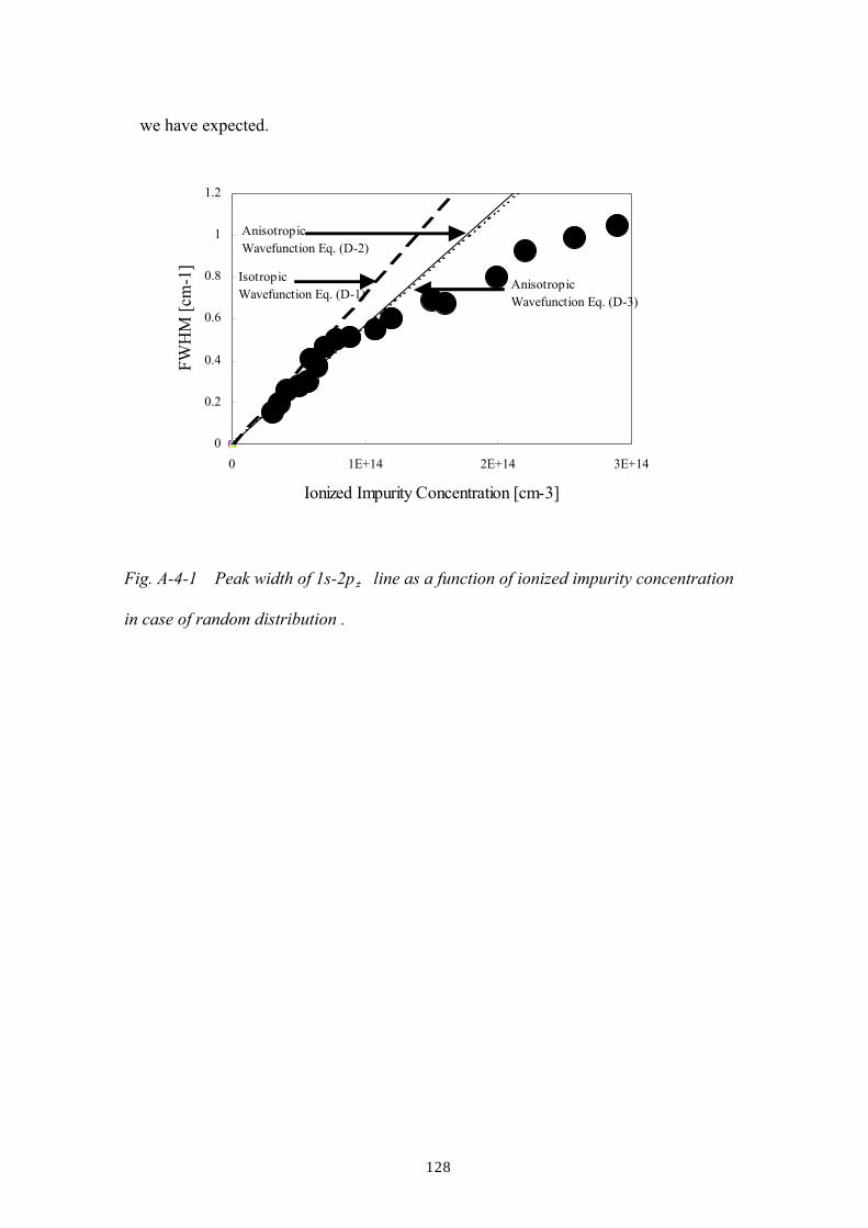
128
we have expected.
0
0.2
0.4
0.6
0.8
1
1.2
0 1E+14 2E+14 3E+14
Ionized Impurity Concentration [cm-3]
FWH
M [c
m-1
]
AnisotropicWavefunction Eq. (D-2)
IsotropicWavefunction Eq. (D-1)
AnisotropicWavefunction Eq. (D-3)
Fig. A-4-1 Peak width of 1s-2p± line as a function of ionized impurity concentration
in case of random distribution .

129
A.5. Monte Carlo methods for the linewidth calculations
This section shows how we have calculated the linewidth of the arsenic (As)
absorption from the ground to 2p± excited states assuming either random or
correlated distributions of the ionized impurities. The energy of the 2p± excited
state of the light-absorbing As shifts due to the electric field arising from either
randomly or correlatingly distributed ionized centers. For the case of n-type Ge at
low temperatures, some of the donors lose their bound electrons to accepters and
become positively ionized. Also, acceptors that have received electrons from
donors become negatively charged. Therefore, we take into account the
distribution of light-absorbing neutral donors, positively charged donors, and
negatively charged acceptors in our Monte Carlo calculation. The effect of the
electric field on the 2p± excited state of the neutral donor is to be found for the
calculation of the linewidth.
In order to find ∆E at one neutral impurity center, 50 donors and 30 acceptors
are randomly distributed in the (x,y,z) space of a single unit cell for the Monte Carlo
calculation. We used linear congruential method to obtain random numbers in our
calculation. 30 donors and acceptors are ionized while 20 donors remain
electrically neutral. The positions of i-th ionized donors and accepters are given by
the coordinates ,, ______ idonorionizedidonorionizedidonorionized zyx and ,, ___ iaccepteriaccepteriaccepter zyx ,
respectively. The compensation ratio 0.6 (= 30 acceptors / 50 donors in a unit cell)
reflects our experiment very well. We have varied the number of donors in the cell
from 10 to 800 and repeated the same full-width-at-half-maximum (FWHM)
calculation as shown in Fig. A-5-1. It shows that FWHM saturates for the number
of donors larger than 20. Therefore, our choice of number of donors in the cell, 30,

130
is confirmed to be large enough for the simulation of our experimental results.
The cell in our calculation is a sphere with a radius L = 6.6×10⁻⁵ cm, set by the
condition:
3023
4 3 ×=⋅ INLπ . (A-5-1)
We distributed 2×30 ions (30 negatively ionized acceptors and 30 positively ionized
donors) in a unit cell. A neutral donor located closest in position to the center of
the spherical cell is the one whose energy shift of excited state is to be calculated.
Its location is indicated by the coordinate
,, ______ centerdonorneutralcenterdonorneutralcenterdonorneutral zyx . This neutral donor is considered to
be an absorption center. We define the new coordinate (X, Y, Z), whose origin is
set at the center of the absorption center, with the direction of the Z-axis being in the
direction parallel to that of symmetry axis of the 2p± orbital. The transformation
of the (x,y,z) coordinate to the (X,Y,Z) coordinate is performed by the following
relation.
0
20
40
60
80
100
120
140
1 10 100 1000 10000
The number of donors in a cell
FWH
M [c
m-1
]
Fig. A-5-1 FWHM vs. the number of the donors in a unit cell. We found the
unit cell containing 50 donors is enough large for our calculation.
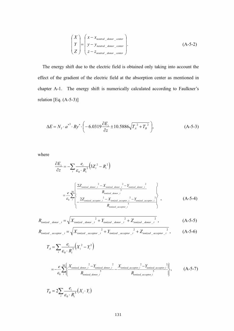
131
−−−
=
centerdonorneutral
centerdonorneutral
centerdonorneutral
zzyyxx
ZYX
__
__
__
. (A-5-2)
The energy shift due to the electric field is obtained only taking into account the
effect of the gradient of the electric field at the absorption center as mentioned in
chapter A-1. The energy shift is numerically calculated according to Faulkner’s
relation [Eq. (A-5-3)]
+±
∂∂
−⋅⋅⋅=∆ 22*3* 5886.100319.6 BAz
I TTz
ERyaNE , (A-5-3)
where
, (A-5-4)
2__
2__
2____ idonorionizedidonorionizedidonorionizedidonorionized ZYXR ++= , (A-5-5)
2__
2__
2____ iacceptorionizediacceptorionizediacceptorionizediacceptorionized ZYXR ++= , (A-5-6)
( )∑ −⋅
=i
iii
iA YX
ReT 22
50ε
∑
−
−−
−=30
5__
2__
2__
5__
2__
2__
0 i iacceptorionized
iaccepterionizediaccepterionized
idonorionized
idonorionizedidonorionized
RYX
RYXe
ε, (A-5-7)
( )∑ ⋅⋅
=i
iii
iB YX
ReT 5
0
2ε
( )∑ −⋅
−=∂∂
iii
i
iz RZR
ez
E 225
0
3ε
∑
−−−
−−
=30
5__
2__
2__
2__
5__
2__
2__
2__
0 2
2
i
iacceptorionized
iaccepterionizediaccepterionizediaccepterionized
idonorionized
idonorionizedidonorionizedidonorionized
RYXZ
RYXZ
eε

132
∑
⋅
−⋅
−=30
5__
____5
__
____
0
2i iacceptorionized
iaccepterionizediaccepterionized
idonorionized
idonorionizedidonorionized
RYX
RYXe
ε,(A-5-8)
where ε0 is the static dielectric constant and ei is the charge of the i-th ion,
Ri(Xi,Yi,Zi) is the distances between ionized impurities and the absorption center.
By the above-mentioned calculation, one energy shift at one absorption center is
obtained in case of the random distribution.
When we calculate the linewidth for the case of the correlated distribution of
ionized impurities, the psuedoground state of the total Coulombic energy in the unit
cell is obtained by changing the distribution of ionized and neutral impurities. A
pair of one neutral donor and one ionized donor is selected randomly and the change
in the total Coulombic energy of the whole cell is calculated as a result of the
electron exchange within the selected pair.
−+= ∑ ∑∑∑∑∑
−+=+=
na
i
na
i
na
j accepterionizedaccepterionized
na
ij accepterionized
na
i
na
ij donorionized rrreEnergyCoulombicTotal
__1 _1 _0
2 1114
__πε
,
(A-5-9)
where
( ) ( ) ( )2____2
____2
_____ jdonorionizedidonorionizedjdonorionizedidonorionizedjdonorionizedidonorionizeddonorionized zzyyxxr −+−+−= ,
(A-5-10)
accepterionizedr _
( ) ( ) ( )2____2
____2
____ jaccepterionizediaccepterionizedjaccepterionizediaccepterionizedjaccepterionizediaccepterionized zzyyxx −+−+−=
. (A-5-11)
accepterionizeddonorionizedr __ −
( ) ( ) ( )2____2
____2
____ jaccepterionizedidonorionizedjaccepterionizedidonorionizedjaccepterionizedidonorionized zzyyxx −+−+−=
. (A-5-12)
133
We accept a new distribution of the ionized and neutral impurities if the energy
is reduced as a result of the electron exchange within the pair, and reject the new
distribution if the energy is increased. This trial is repeated for 3000 times in order
to obtain the psuedground state of the correlated distribution of impurities. Fig.
A-5-2 shows the change in the total Coulombic energy as a function of the number
of trials. It shows that the psuedground state is obtained for a trial of more than 100
times, i.e., our calculation using 3000 trials is more than sufficient. The program
code for these linewidth calculations in case of random distribution and correlated
distribution is written in Appendix E.
The linewidth for the both cases of the random and correlated distribution have
been obtained by repeating above-mentioned routines for 30,000 times, i.e., Monte
Carlo results shown in Fig. A-5-2 of the manuscript is composed of 30,000 Monte
Carlo data, though we do not show all of them in the plot. Figure A-5-3 shows
distributions of ionized donors, neutral donors, and acceptors in a calculational cell
in case of random distribution and correlated distribution (after we obtained
psuedground state of the total Coulombic energy) when 800 donors and 400
acceptors are randomly distributed in a cell.
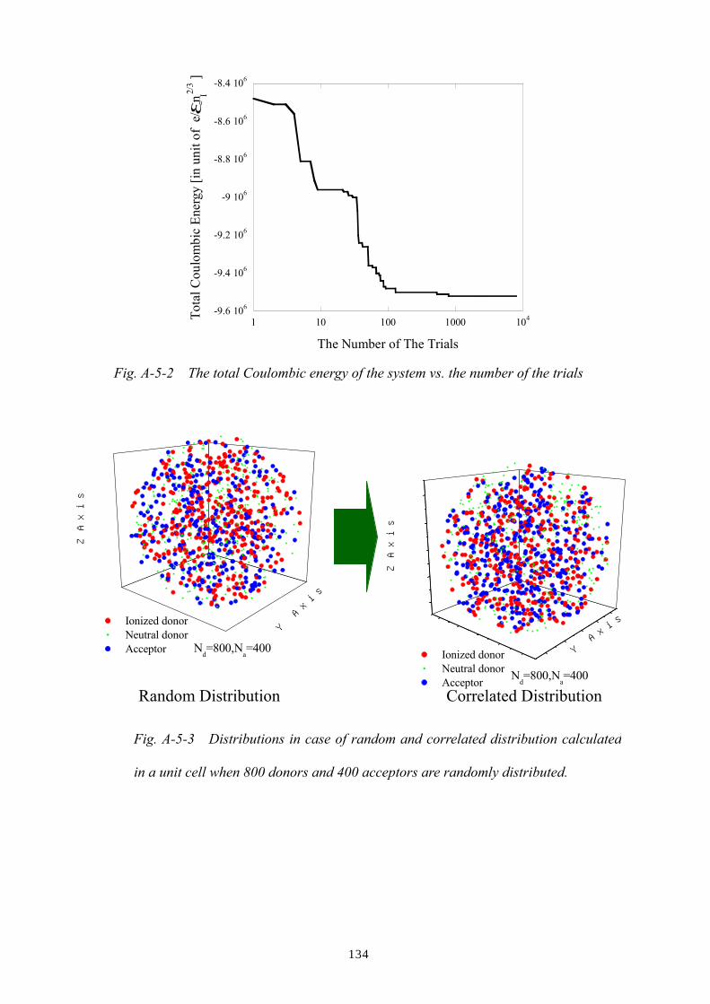
134
Fig. A-5-2 The total Coulombic energy of the system vs. the number of the trials
Nd=800,N
a=400
Ionized donor Neutral donor Acceptor
Y Axis
Z A
xis
Nd=800,N
a=400
Ionized donor Neutral donor Acceptor
Y Axis
Z A
xis
Random Distribution Correlated Distribution
Fig. A-5-3 Distributions in case of random and correlated distribution calculated
in a unit cell when 800 donors and 400 acceptors are randomly distributed.
-9.6 106
-9.4 106
-9.2 106
-9 106
-8.8 106
-8.6 106
-8.4 106
1 10 100 1000 104Tota
l Cou
lom
bic
Ener
gy [i
n un
it of
e/
nI2/
3 ]
The Number of The Trials
0

135
References
1 D. M. Larsen, Phys. Rev. B 13, 1681 (1976).
2 Kohn and J. M. Luttinger, Phys. Rev. 98, 915 (1955).
3 R. A. Faulkner, Phys. Rev. 184, 713 (1969).

136
Appendix B: Calculation for energy of 1s orbital in Ge according to
Kohn-Luttinger method
Clear@a, b, γDγ = 0.05134;amin= 0.5;bmin= 0.5;Mimimumvalue= 100000;
sorbital:=1è
π ×a2 × b×
−$ q2a2 + z2
b2
ForAi= 1, i< 200, i++,a= amin+ amin∗HRandom@D − 0.5Lê0.5∗ 0.5í è i;b= bmin+ bmin∗HRandom@D − 0.5Lê0.5∗ 0.5í è i;totalenergy=
NA·
−∞
∞·0
∞ik −2$ q2
a2 + z2b2 ik−b4 q2ik2a2 $ q2
a2 +z2b2 +
è q2 + z2 ik−1+$ q2a2 +
z2b2
yy−
a4z2 è q2 + z2 $ q2a2 +
z2b2 γ +
a2 b2 ik2z2ikè q2 + z2 − a2 $ q2a2 +
z2b2
y + q2è q2 + z2 γyyy ì
ika4 b3 πè q2 + z2 Ib2 q2 + a2z2M$ q2
a2 +z2b2
y×2 π ×q q zE;
If@Mimimumvalue> totalenergy, amin= a, amin= aminDIf@Mimimumvalue> totalenergy, bmin= b, bmin= bminDIf@Mimimumvalue> totalenergy, Mimimumvalue= totalenergy,
Mimimumvalue= MimimumvalueDPrint@i, " ", Mimimumvalue, " ", totalenergy, " ", amin, " ",
bmin, " ", a, " ", bDE
(A programming code for Mathmatica)

137
Appendix C: Calculation for energy of 2p(m=1) orbital in Ge according to
Kohn-Luttinger method
Clear@a, b, γDγ = 0.051340; H∗ γ=m1êm2∗Lamin= 1.5; H∗ initial value of variable coefficient ∗Lbmin= 0.5; H∗ initial value of variable coefficient ∗LMimimumvalue= 1000000;
porbital:=xè
π ×a4 × b1×
−$ x2+y2a2 + z2
b2
H∗ a wavefunction of p−orbital ∗LH∗ finding the minimum eigenvalues of wavefunctions ∗LForAi= 1, i< 200, i++,a= amin+ amin∗HRandom@D − 0.5Lê0.5∗ 0.5í è i;b= bmin+ bmin∗HRandom@D − 0.5Lê0.5∗ 0.5í è i;totalenergy=
NA‡−∞
∞‡−∞
∞‡−∞
∞ikporbital×ik−γ × D@D@porbital, zD, zD− D@D@porbital, xD, xD−
D@D@porbital, yD, yD −2è x2 + y2 +z2
× porbitalyy x y zE;
If@Mimimumvalue> totalenergy, amin= a, amin= aminDIf@Mimimumvalue> totalenergy, bmin= b, bmin= bminDIf@Mimimumvalue> totalenergy, Mimimumvalue= totalenergy,
Mimimumvalue= MimimumvalueDPrint@i, " ", Mimimumvalue, " ", totalenergy, " ", amin," ", bmin, " ", a, " ", bDE
a= amin;b= bmin;NA‡
−∞
∞‡−∞
∞‡−∞
∞Iporbital×I2 z2 −x2 − y2M× porbitalM x y zENA‡
−∞
∞‡−∞
∞‡−∞
∞Iporbital×Ix2 +y2M× porbitalM x y zE
(A programming code for Mathmatica)

138
Appendix D: Calculation for energies of orbitals in Ge according to Faulkner’s
method
Clear@n, l, m, α1, α2, α3, β, γ, p, k, rDγ = 0.05134; H∗ γ=m1êm2∗Lα1min= 1.38524; H∗ initial value of variable coefficient ∗Lα3min= 1.38524; H∗ initial value of variable coefficient ∗Lα5min= 1.38524; H∗ initial value of variable coefficient ∗Lβmin= 0.156499; H∗ initial value of variable coefficient ∗LMimimumvalue= 10000000000;
rnl1@n_D :=2 α132
n2 ×ik Hn− 1− 1L!HHn+ 1L!L3
y0.5×J 2 α1×r
n N×− α1×rn ×lpk1@n− 2, 3, nDH∗ tadial wavefunction for l=1 ∗L
rnl3@n_D :=2 α332
n2 ×ik Hn− 3− 1L!HHn+ 3L!L3
y0.5×J 2 α3×r
n N3×
− α3×rn ×lpk3@n− 4, 7, nDH∗ tadial wavefunction for l=3 ∗Lrnl5@n_D :=
2 α532n2 ×
ik Hn− 5− 1L!HHn+ 5L!L3y0.5
×J 2 α5×rn N5
×− α5×rn ×lpk5@n− 6, 11, nDH∗ tadial wavefunction for l=5 ∗L
lpk1@p_, k_, n_D :=„s=0
p H−1Ls ×HHp+ kL!L2Hp−sL!×Hk+ sL!×s!
×J 2 α1×rn Ns
H∗ Legendre function for l=1 ∗Llpk3@p_, k_, n_D :=„
s=0
p H−1Ls ×HHp+ kL!L2Hp−sL!×Hk+ sL!×s!
×J 2 α3×rn Ns
H∗ Legendre function for l=3 ∗Llpk5@p_, k_, n_D :=„
s=0
p H−1Ls ×HHp+ kL!L2Hp−sL!×Hk+ sL!×s!
×J 2 α5×rn Ns
H∗ Legendre function for l=5 ∗Lylm@l_, m_D := H−1L m+Abs@mD
2 ×$ 2×l+ 14 π
×H1− Abs@mDL!H1+ Abs@mDL!
×
LegendreP@l, Abs@mD, Cos@θDD H∗ spherical harmonics ∗Lil1l2@l1_, l2_, m_D := ·
0
2 π·0
π ylm@l1, mD×ylm@l2, mD$1− I1− γβM×HCos@θDL2
×Sin@θD θ φ
(A programming code for Mathmatica)

139
H∗ R.A.Faulkner' s equation H2.14L ∗Lj011@n1_, n2_D := ‡0
∞rnl1@n1D×rnl1@n2D rH∗ R.A.Faulkner' s equation H2.15L for l=1 and l'=1 ∗Lj013@n1_, n2_D := ‡0
∞rnl1@n1D×rnl3@n2D rH∗ R.A.Faulkner' s equation H2.15L for l=1 and l'=3 ∗Lj015@n1_, n2_D := ‡0
∞rnl1@n1D×rnl5@n2D rH∗ R.A.Faulkner' s equation H2.15L for l=1 and l'=5 ∗Lj031@n1_, n2_D := ‡0
∞rnl3@n1D×rnl1@n2D rH∗ R.A.Faulkner' s equation H2.15L for l=3 and l'=1 ∗Lj033@n1_, n2_D := ‡0
∞rnl3@n1D×rnl3@n2D rH∗ R.A.Faulkner' s equation H2.15L for l=3 and l'=3 ∗Lj035@n1_, n2_D := ‡0
∞rnl3@n1D×rnl5@n2D rH∗ R.A.Faulkner' s equation H2.15L for l=3 and l'=5 ∗Lj051@n1_, n2_D := ‡0
∞rnl5@n1D×rnl1@n2D rH∗ R.A.Faulkner' s equation H2.15L for l=5 and l'=1 ∗Lj053@n1_, n2_D := ‡0
∞rnl5@n1D×rnl3@n2D rH∗ R.A.Faulkner' s equation H2.15L for l=5 and l'=3 ∗Lj055@n1_, n2_D := ‡0
∞rnl5@n1D×rnl5@n2D rH∗ R.A.Faulkner' s equation H2.15L for l=5 and l'=5 ∗Lj111@n1_, n2_D := ‡0
∞r×rnl1@n1D ×rnl1@n2D rH∗ R.A.Faulkner' s equation H2.16L for l=1 and l'=1 ∗Lj113@n1_, n2_D := ‡0
∞r×rnl1@n1D ×rnl3@n2D rH∗ R.A.Faulkner' s equation H2.16L for l=1 and l'=3 ∗Lj115@n1_, n2_D := ‡0
∞r×rnl1@n1D ×rnl5@n2D rH∗ R.A.Faulkner' s equation H2.16L for l=1 and l'=5 ∗Lj131@n1_, n2_D := ‡0
∞r×rnl3@n1D ×rnl1@n2D rH∗ R.A.Faulkner' s equation H2.16L for l=3 and l'=1 ∗Lj133@n1_, n2_D := ‡0
∞r×rnl3@n1D ×rnl3@n2D rH∗ R.A.Faulkner' s equation H2.16L for l=3 and l'=3 ∗Lj135@n1_, n2_D := ‡0
∞r×rnl3@n1D ×rnl5@n2D rH∗ R.A.Faulkner' s equation H2.16L for l=3 and l'=5 ∗Lj151@n1_, n2_D :=‡0
∞r×rnl5@n1D× rnl1@n2D rH∗ R.A.Faulkner' s equation H2.16L for l=5 and l'=1 ∗L

140
j153@n1_, n2_D := ‡0∞r×rnl5@n1D ×rnl3@n2D rH∗ R.A.Faulkner' s equation H2.16L for l=5 and l'=3 ∗L
j155@n1_, n2_D := ‡0∞r×rnl5@n1D ×rnl5@n2D rH∗ R.A.Faulkner' s equation H2.16L for l=5 and l'=5 ∗L
j211@n1_, n2_D := ‡0∞r2 ×rnl1@n1D×rnl1@n2D rH∗ R.A.Faulkner' s equation H2.17L for l=1 and l'=1 ∗L
j213@n1_, n2_D := ‡0∞r2 ×rnl1@n1D×rnl3@n2D rH∗ R.A.Faulkner' s equation H2.17L for l=1 and l'=3 ∗L
j215@n1_, n2_D := ‡0∞r2 ×rnl1@n1D×rnl5@n2D rH∗ R.A.Faulkner' s equation H2.17L for l=1 and l'=5 ∗L
j231@n1_, n2_D := ‡0∞r2 ×rnl3@n1D×rnl1@n2D rH∗ R.A.Faulkner' s equation H2.17L for l=3 and l'=1 ∗L
j233@n1_, n2_D := ‡0∞r2 ×rnl3@n1D×rnl3@n2D rH∗ R.A.Faulkner' s equation H2.17L for l=3 and l'=3 ∗L
j235@n1_, n2_D := ‡0∞r2 ×rnl3@n1D×rnl5@n2D rH∗ R.A.Faulkner' s equation H2.17L for l=3 and l'=5 ∗L
j251@n1_, n2_D := ‡0∞r2 ×rnl5@n1D×rnl1@n2D rH∗ R.A.Faulkner' s equation H2.17L for l=5 and l'=1 ∗L
j253@n1_, n2_D := ‡0∞r2 ×rnl5@n1D×rnl3@n2D rH∗ R.A.Faulkner' s equation H2.17L for l=5 and l'=3 ∗L
j255@n1_, n2_D := ‡0∞r2 ×rnl5@n1D×rnl5@n2D rH∗ R.A.Faulkner' s equation H2.17L for l=5 and l'=5 ∗L
d11@n1_, n2_D := ‡0∞r×rnl1@n1D × D@rnl1@n2D, rD rH∗ R.A.Faulkner' s equation H2.18L for l=1 and l'=1 ∗L
d13@n1_, n2_D := ‡0∞r×rnl1@n1D × D@rnl3@n2D, rD rH∗ R.A.Faulkner' s equation H2.18L for l=1 and l'=3 ∗L
d15@n1_, n2_D := ‡0∞r×rnl1@n1D × D@rnl5@n2D, rD rH∗ R.A.Faulkner' s equation H2.18L for l=1 and l'=5 ∗L
d31@n1_, n2_D := ‡0∞r×rnl3@n1D × D@rnl1@n2D, rD rH∗ R.A.Faulkner' s equation H2.18L for l=3 and l'=1 ∗L
d33@n1_, n2_D := ‡0∞r×rnl3@n1D × D@rnl3@n2D, rD rH∗ R.A.Faulkner' s equation H2.18L for l=3 and l'=3 ∗L
d35@n1_, n2_D :=‡0∞r×rnl3@n1D× D@rnl5@n2D, rD rH∗ R.A.Faulkner' s equation H2.18L for l=3 and l'=5 ∗L

141
d51@n1_, n2_D := ‡0∞r×rnl5@n1D × D@rnl1@n2D, rD rH∗ R.A.Faulkner' s equation H2.18L for l=5 and l'=1 ∗L
d53@n1_, n2_D := ‡0∞r×rnl5@n1D × D@rnl3@n2D, rD rH∗ R.A.Faulkner' s equation H2.18L for l=5 and l'=3 ∗L
d55@n1_, n2_D := ‡0∞r×rnl5@n1D × D@rnl5@n2D, rD rH∗ R.A.Faulkner' s equation H2.18L for l=5 and l'=5 ∗L
hl1l1@n_, m_D :=
ReA−2×il1l2@1, 1, mD×j111@n, nD +ik1− H1− βL×13 ×
ik1+2×1× H1+ 1L − 6× m2H2×1− 1L×H2×1+ 3L yy ×
ik−Hα1L2
n2 + 2×α1×j111@n, nDyEhl1l1n@n1_, n2_, m_D :=
ReA−2×il1l2@1, 1, mD×j111@n1, n2D +ik1− H1− βL×13 ×
ik1+2×1× H1+ 1L − 6× m2H2×1− 1L×H2×1+ 3L yy ×H2×α1×j111@n1, n2DLE
hl3l3@n_, m_D :=
ReA−2×il1l2@3, 3, mD×j133@n, nD +ik1− H1− βL×13 ×
ik1+2×3× H3+ 1L − 6× m2H2×3− 1L×H2×3+ 3L yy ×
ik−Hα3L2
n2 + 2×α3×j133@n, nDyEhl3l3n@n1_, n2_, m_D :=
ReA−2×il1l2@3, 3, mD×j133@n1, n2D +ik1− H1− βL×13 ×
ik1+2×3× H3+ 1L − 6× m2H2×3− 1L×H2×3+ 3L yy ×H2×α3×j133@n1, n2DLE
hl5l5@n_, m_D :=
ReA−2×il1l2@5, 5, mD×j155@n, nD +ik1− H1− βL×13 ×
ik1+2×5× H5+ 1L − 6× m2H2×5− 1L×H2×5+ 3L yy ×
ik−Hα5L2
n2 + 2×α5×j155@n, nDyEhl5l5n@n1_, n2_, m_D :=
ReA−2×il1l2@5, 5, mD×j155@n1, n2D +ik1− H1− βL×13 ×
ik1+2×5× H5+ 1L − 6× m2H2×5− 1L×H2×5+ 3L yy ×H2×α5×j155@n1, n2DLEH∗ R.A.Faulkner' s equationH2.19L for Hl,l'L=H1,1L,H3,3L,and H5,5L ∗L
hl1l3@n1_, n2_, m_D :=
ReA−2 il1l2@1, 3, mD×j113@n1, n2D +H1− βL×1
2×3− 1 ×$ H32 − m2L×HH3− 1L2 − m2LH2×3+ 1L×H2×3− 3L ×ik 12 ×
ik α32n22 +
α12n12
y×j213@n1, n2D− Hα3+ α1L×j113@n1, n2D +
3×H2×3− 1L×j013@n1, n2D + H2×3− 1L×d13@n1, n2DyEhl3l1@n1_, n2_, m_D :=
ReA−2 il1l2@1, 3, mD×j113@n1, n2D + H1− βL×1
2×3− 1 ×$ H32 − m2L×HH3− 1L2 − m2LH2×3+ 1L×H2×3− 3L ×

142
ik 12 ×
ik α12n22 +
α32n12
y×j231@n1, n2D− Hα3+ α1L×j131@n1, n2D + 3×H2×3− 1L×j031@n1, n2D +H2×3−1L ×d31@n1, n2DyEhl3l5@n1_, n2_, m_D :=
ReA−2 il1l2@3, 5, mD×j135@n1, n2D +H1− βL×1
2×5− 1 ×$ H52 − m2L×HH5− 1L2 − m2LH2×5+ 1L×H2×5− 3L ×ik 12 ×
ik α52n22 +
α32n12
y×j235@n1, n2D− Hα5+ α3L×j135@n1, n2D +
5×H2×5− 1L×j035@n1, n2D + H2×5− 1L×d35@n1, n2DyEhl5l3@n1_, n2_, m_D :=
ReA−2 il1l2@5, 3, mD×j153@n1, n2D +H1− βL×1
2×5− 1 ×$ H52 − m2L×HH5− 1L2 − m2LH2×5+ 1L×H2×5− 3L ×ik 12 ×
ik α52n22 +
α32n12
y×j253@n1, n2D− Hα5+ α3L×j153@n1, n2D +
5×H2×5− 1L×j053@n1, n2D + H2×5− 1L×d53@n1, n2DyEH∗ R.A.Faulkner' s equationH2.19L for Hl,l'L=H1,3L,H3,1L,H3,5L,and H5,3L ∗Lhl1l5@n1_, n2_, m_D := Re@−2×il1l2@1, 5, mD×j115@n1, n2DDhl151@n1_, n2_, m_D := Re@−2×il1l2@5, 1, mD×j151@n1, n2DDH∗ R.A.Faulkner' s equationH2.19L for Hl,l'L=H1,5L and H5,1L ∗Ltensol:=88hl1l1@2, 1D, hl1l1n@2, 3, 1D, hl1l1n@2, 4, 1D, hl1l1n@2, 5, 1D, hl1l1n@2, 6, 1D,
hl1l1n@2, 7, 1D<,8hl1l1n@3, 2, 1D, hl1l1@3, 1D, hl1l1n@3, 4, 1D, hl1l1n@3, 5, 1D, hl1l1n@3, 6, 1D,hl1l1n@3, 7, 1D<,8hl1l1n@4, 2, 1D, hl1l1n@4, 3, 1D, hl1l1@4, 1D, hl1l1n@4, 5, 1D, hl1l1n@4, 6, 1D,hl1l1n@4, 7, 1D<,8hl1l1n@5, 2, 1D, hl1l1n@5, 3, 1D, hl1l1n@5, 4, 1D, hl1l1@5, 1D, hl1l1n@5, 6, 1D,hl1l1n@5, 7, 1D<,8hl1l1n@6, 2, 1D, hl1l1n@6, 3, 1D, hl1l1n@6, 4, 1D, hl1l1n@6, 5, 1D,hl1l1@6, 1D, hl1l1n@6, 7, 1D<,8hl1l1n@7, 2, 1D, hl1l1n@7, 3, 1D, hl1l1n@7, 4, 1D, hl1l1n@7, 5, 1D,hl1l1n@7, 6, 1D, hl1l1@7, 1D<<
H∗ finding the minimum eigenvalues of wavefunctions ∗LForAi= 1, i< 200, i++,α1= α1min+ α1min∗HRandom@D − 0.5Lê0.5∗ 0.3í è i;α3= α3min+ α3min∗HRandom@D − 0.5Lê0.5∗ 0.3í è i;
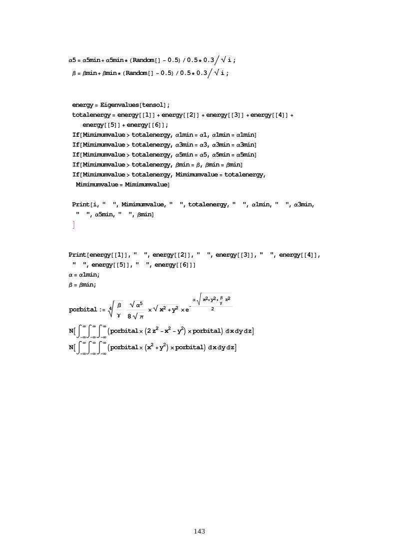
143
α5= α5min+ α5min∗HRandom@D − 0.5Lê0.5∗ 0.3í è i;β = βmin+ βmin∗HRandom@D − 0.5Lê0.5∗ 0.3í è i;
energy= Eigenvalues@tensolD;totalenergy= energy@@1DD+ energy@@2DD + energy@@3DD +energy@@4DD +
energy@@5DD+ energy@@6DD;If@Mimimumvalue> totalenergy, α1min= α1, α1min= α1minDIf@Mimimumvalue> totalenergy, α3min= α3, α3min= α3minDIf@Mimimumvalue> totalenergy, α5min= α5, α5min= α5minDIf@Mimimumvalue> totalenergy, βmin= β, βmin= βminDIf@Mimimumvalue> totalenergy, Mimimumvalue= totalenergy,
Mimimumvalue= MimimumvalueDPrint@i, " ", Mimimumvalue, " ", totalenergy, " ", α1min, " ", α3min," ", α5min, " ", βminDE
Print@energy@@1DD, " ", energy@@2DD, " ", energy@@3DD, " ", energy@@4DD," ", energy@@5DD, " ", energy@@6DDD
α = α1min;β = βmin;
porbital:= $ β
γ4
èα5
8 è
π×è x2 +y2 ×
−
α $ x2+y2+ βγ
z22
NA‡−∞
∞‡−∞
∞‡−∞
∞Iporbital×I2 z2 −x2 − y2M× porbitalM x y zENA‡
−∞
∞‡−∞
∞‡−∞
∞Iporbital×Ix2 +y2M× porbitalM x y zE

144
Appendix E: Calculation for linewidths of 1s-2p lines in the case of random and
correlated distribution
#include <stdio.h>
#include <stdlib.h>
#include <time.h>
#include <math.h>
main(void)
int change, p, q, number_of_data, number_of_trial,
i, j, m, number_of_accepter, number_of_donor,
randoma, randomb, a[20], b[30];
double ta, tb, field_gradient, random, ionized_impurity_concentration,
distance_ionized_donor, distance_ionized_accepter, ezero, electon, azero,
cmnx, cmny, cmnz, kyori, energyaa,
unit_length, minimum_energy, coulomb_energy, ans_plus, ans_minus,
ionized_donor_x[30], ionized_donor_y[30], ionized_donor_z[30],
ionized_accepter_x[30], ionized_accepter_y[30], ionized_accepter_z[30],
donor_x[50], donor_y[50], donor_z[50],
accepter_x[30], accepter_y[30], accepter_z[30];
ezero = 1.0;
azero = 87.6e-8;
(A programming code for C language)

145
electon = 4.8e-10;
number_of_accepter = 30;
number_of_donor = 50;
ionized_impurity_concentration = 5.0e13;
unit_length = pow(3.0/2.0/3.141592654*number_of_accepter/ionized_impurity_concentration,1.0/3.0);
srand(time(NULL));
printf("number_of_donor = %d number_of_accepter = %d ionized_impurity_concentration = %g azero = %g ¥n",
number_of_donor, number_of_accepter, ionized_impurity_concentration, azero);
/* a routine for obtain 30000 data */
for (number_of_data=0; number_of_data<30000; number_of_data++)
minimum_energy = 1.0e100;
/* making a distribution of donors and acceptors randomly */
i = 0;
while ( i<number_of_donor )
random = rand();
donor_x[i] = random / 32768.0 * 2.0 * unit_length - unit_length;
random = rand();
donor_y[i] = random / 32768.0 * 2.0 * unit_length - unit_length;
random = rand();
donor_z[i] = random / 32768.0 * 2.0 * unit_length - unit_length;
if ( pow(donor_x[i],2.0)+pow(donor_y[i],2.0)+pow(donor_z[i],2.0) <
pow(unit_length,2.0) )
i = i+1 ;
146
i = 0;
while ( i<number_of_accepter )
random = rand();
accepter_x[i] = random / 32768.0 * 2.0 * unit_length - unit_length;
random = rand();
accepter_y[i] = random / 32768.0 * 2.0 * unit_length - unit_length;
random = rand();
accepter_z[i] = random / 32768.0 * 2.0 * unit_length - unit_length;
if ( pow(accepter_x[i],2.0)+pow(accepter_y[i],2.0)+pow(accepter_z[i],2.0) <
pow(unit_length,2.0) )
i = i+1 ;
/* Coulombic energy between acceptors */
energyaa = 0;
for( i=0; i<number_of_accepter; i++)
for( j=0; j<number_of_accepter; j++)
if ( i > j)
energyaa = energyaa +
1.0/pow(pow(accepter_x[i]-accepter_x[j],2.0)+pow(accepter_y[i]-accepter_y[j],2.0)+pow(accepter_z[i]-accepter_z[j],2.0),0.5);
/* decidion of a distribution of ionizd donors */
i=0;
147
while ( i < number_of_donor - number_of_accepter )
randoma = rand() % number_of_donor;
a[i] = randoma;
q=0;
for ( p=0; p<i; p++)
if ( a[i] == a[p]) q = q+1;
if ( q == 0 ) i = i+1;
m = 0;
while ( m < number_of_accepter)
for (i=0; i< number_of_donor ; i++)
p=0;
for (j=0; j<number_of_donor - number_of_accepter; j++)
if ( i == a[j] ) p = p+1;
if (p==0)
b[m] = i;
m++;
/* a routine for making a correlated distribution */
for (number_of_trial=0; number_of_trial<3000; number_of_trial++)

148
randoma = rand() % (number_of_donor - number_of_accepter);
change = a[randoma];
randomb = rand() % number_of_accepter;
a[randoma] = b[randomb];
b[randomb] = change;
if(number_of_trial==0)
coulomb_energy = energyaa;
for( i = 0; i < number_of_accepter; i++)
for( j = 0; j < number_of_accepter; j++)
if ( i < j)
coulomb_energy =
coulomb_energy +
1.0/pow(pow(donor_x[b[i]]-donor_x[b[j]],2.0)+pow(donor_y[b[i]]-donor_y[b[j]],2.0)+pow(donor_z[b[i]]-donor_z[b[j]],2.0),0.
5);
for( i = 0; i < number_of_accepter; i++)
for( j = 0; j < number_of_accepter; j++)
coulomb_energy = coulomb_energy -
1.0/pow(pow(donor_x[b[i]]-accepter_x[j],2.0)+pow(donor_y[b[i]]-accepter_y[j],2.0)+pow(donor_z[b[i]]-accepter_z[j],2.0),0.5
);

149
if(number_of_trial > 0)
coulomb_energy = minimum_energy;
for(j=0 ; j<number_of_accepter ; j++)
if(j!=randomb)
coulomb_energy = coulomb_energy +
1.0/pow(pow(donor_x[b[randomb]]-donor_x[b[j]],2.0)+pow(donor_y[b[randomb]]-donor_y[b[j]],2.0)+pow(donor_z[b[random
b]]-donor_z[b[j]],2.0),0.5) -
1.0/pow(pow(donor_x[a[randoma]]-donor_x[b[j]],2.0)+pow(donor_y[a[randoma]]-donor_y[b[j]],2.0)+pow(donor_z[a[random
a]]-donor_z[b[j]],2.0),0.5);
coulomb_energy = coulomb_energy -
1.0/pow(pow(donor_x[b[randomb]]-accepter_x[j],2.0)+pow(donor_y[b[randomb]]-accepter_y[j],2.0)+pow(donor_z[b[random
b]]-accepter_z[j],2.0),0.5) +
1.0/pow(pow(donor_x[a[randoma]]-accepter_x[j],2.0)+pow(donor_y[a[randoma]]-accepter_y[j],2.0)+pow(donor_z[a[randoma
]]-accepter_z[j],2.0),0.5);
if ( minimum_energy > coulomb_energy )
minimum_energy = coulomb_energy;
else
change = a[randoma];
a[randoma] = b[randomb];
b[randomb] = change;
150
/* close a routine for making a correlated distribution */
/* decision of the neutral impurity which locates center of the unit cell */
kyori = 2*unit_length;
for (i=0; i < number_of_donor - number_of_accepter; i++)
if ( kyori >
pow(pow(donor_x[a[i]],2)+pow(donor_y[a[i]],2)+pow(donor_z[a[i]],2),0.5) )
kyori =
pow(pow(donor_x[a[i]],2)+pow(donor_y[a[i]],2)+pow(donor_z[a[i]],2),0.5);
cmnx = donor_x[a[i]];
cmny = donor_y[a[i]];
cmnz = donor_z[a[i]];
/* calculation of the energy shift */
field_gradient = 0.0;
ta = 0.0;
tb = 0.0;
for (i=0; i < number_of_accepter; i++)
ionized_donor_x[i] = (donor_x[b[i]]-cmnx);
ionized_donor_y[i] = (donor_y[b[i]]-cmny);
ionized_donor_z[i] = (donor_z[b[i]]-cmnz);
ionized_accepter_x[i] = (accepter_x[i]-cmnx);
151
ionized_accepter_y[i] = (accepter_y[i]-cmny);
ionized_accepter_z[i] = (accepter_z[i]-cmnz);
distance_ionized_donor =
pow(ionized_donor_x[i]*ionized_donor_x[i]+ionized_donor_y[i]*ionized_donor_y[i]+ionized_donor_z[i]*ionized_donor_z[i],
0.5);
distance_ionized_accepter =
pow(ionized_accepter_x[i]*ionized_accepter_x[i]+ionized_accepter_y[i]*ionized_accepter_y[i]+ionized_accepter_z[i]*ionized
_accepter_z[i],0.5);
field_gradient = field_gradient +
(1.0/pow(distance_ionized_donor,5.0)*(3.0*pow(ionized_donor_z[i],2.0)-pow(distance_ionized_donor,2.0))-1.0/pow(distance_
ionized_accepter,5.0)*(3.0*pow(ionized_accepter_z[i],2.0)-pow(distance_ionized_accepter,2.0)))/ionized_impurity_concentrat
ion;
ta = ta +
(-1.0/pow(distance_ionized_donor,5.0)*(pow(ionized_donor_x[i],2.0)-pow(ionized_donor_y[i],2.0))+1/pow(distance_ionized_
accepter,5.0)*(pow(ionized_accepter_x[i],2.0)-pow(ionized_accepter_y[i],2.0)))/ionized_impurity_concentration;
tb = tb +
(-2.0/pow(distance_ionized_donor,5.0)*ionized_donor_x[i]*ionized_donor_y[i]+2.0/pow(distance_ionized_accepter,5.0)*ioniz
ed_accepter_x[i]*ionized_accepter_y[i])/ionized_impurity_concentration;
ans_plus = -6.0319*field_gradient+10.6006*pow(pow(ta,2.0)+pow(tb,2.0),0.5);
ans_minus = -6.0319*field_gradient-10.6006*pow(pow(ta,2.0)+pow(tb,2.0),0.5);
printf("%d, %g, %g¥n", number_of_data, ans_plus, ans_minus);
/* close a routine for obtain 30000 data */
return 0 ;

152
Appendix F: Calculation of one-dimensional harmonic linear chain model
Here, we explain one-dimensional linear chain calculation within harmonic
oscillation, for instance, in case of five atoms (Fig. F-1). From K1 to K5 are force
constants between each atom, and from M1 to M5 are masses of each atom in Fig.
F-1. From u1 to u5 are distances from most stable positions of each atom. Then,
we obtained Eq. (F-1).
( ) ( )( ) ( )( ) ( )( ) ( )( ) ( )
+−++−=+−++−=+−++−=+−++−=+−++−=
15245155
54534444
43423333
32312222
21251111
uuKuuKuMuuKuuKuMuuKuuKuMuuKuuKuMuuKuuKuM
&&
&&
&&
&&
&&
, (F-1)
where, ( )ikxtiCu ii −⋅= ωexp since the vibration is supposed to be hamonic. At
the momentum k is zero, in case we obtained by our absorption measurements, we
use ( )tiCu ii ⋅= ωexp in Eq. (F-1). Then, we obtained Eq. (F-2).
( )( )( )( )
( )
−−++=−+−−+=−+−−+=−+−−+=−++−−=−
515451152
5
554543442
4
443432332
3
332321222
2
512212112
1
uKKuKuKuMuKuKKuKuMuKuKKuKuMuKuKKuKuMuKuKuKKuM
ωωωωω
(F-2)
Using matrix, Eq. (F-2) is expressed as Eq. (F-3).
M1 M2 M3 M5M4
K1 K2 K3 K1 K4 K5
Fig. F-1. A illustration of the linear chain model we used in case of five atoms in a cell.
153
+−−−+−
−+−−+−
−−+
=
5
4
3
2
1
1551
5544
4433
3322
1221
55
44
33
22
11
2
0000
0000
00
uuuuu
KKKKKKKK
KKKKKKKK
KKKK
uMuMuMuMuM
ω (F-3)
For easy calculation, Eq. (F-4) is better expression rather than Eq. (F-3).
+⋅
−⋅
−⋅
−+⋅
−⋅
−+⋅
−⋅
−+⋅
−⋅
−⋅
−+
=
55
44
33
22
11
5
15
45
5
15
1
54
5
4
54
34
4
43
4
3
43
23
3
32
3
2
32
12
2
51
1
21
2
1
21
55
44
33
22
11
2
00
00
00
00
00
uMuMuMuMuM
MKK
MMK
MMK
MMK
MKK
MMK
MMK
MKK
MMK
MMK
MKK
MMK
MMK
MMK
MKK
uMuMuMuMuM
ω
(F-4)
For example, we calculate when mass number of silicon atoms is 28 and that of
oxygen is 16. The masses used are
][1064.4 2628 kgM Si
−×= (=M1, M2, M4, M5)
][1066.2 2616 kgM O
−×= (=M3).
Force constants between Si-Si and Si-O is
]/[18.479 mNK OSi =− and
]/[33.113 mNK SiSi =− ,

154
which are obtained by the Raman measurement and absorption measurements of
isotopically controlled Si as mentioned fore part of this chapter. Calculational
frequencies (ω ) are obtained in unit of [s-1]. To obtain these frequencies in unit of
[cm-1], we multiplied 5.3129×10⁻¹², and then, we obtained these eigenvalues,
ω =1151.51, 615.87, 409.70, 343.539, 147.16 [cm-1]
The eigenfunctions (that mean square of mass times distance from stable position of
atom) for each eigenvalue are as follows,
1 2 3 4 5
1 2 3 4 5 1 2 3 4 5
1 2 3 4 5
1 2 3 4 5
ω =1151.51cm-1 ω =615.87 cm-1
ω =409.70 cm-1 ω =343.538 cm-1
ω =147.16 cm-1
Position
Position Position
Position
Position
Fig. F-2 The dispersion patterns for each eigenvalue in case of 5 atoms (one
oxygen and four silicon atoms) in a unit cell.

155
As you can see, the vibration is strongly localized when eigenvalue is ω =1151.51
[cm-1]. The next step, we did same kind of calculation with 201 atoms (one oxygen
located at the center of the unit cell and 200 silicon atoms around oxygen atom) and
obtained eigenvalues in Fig. F-3. Two higher frequencies obtained in Fig. F-3
indicate the vibration due to A1g and A2u modes from the dispersion patterns in Fig.
F-4 (ω =617cm-1) and F-4 (ω =1151cm-1). Fig. F-3 means density of states of
atomic vibrations in unit cell. The reason why there is continual density of state
under 500 cm-1 is that we used mono force constant between silicon atoms in order
to reduce parameters in our calculation models. We confirmed this effect on LVM
frequencies by comparison with the model with two force constants between silicon
atoms.
0
5
10
15
20
25
60 200 340 480 620 760 900 1040 1180
Cou
nt o
f dat
a
Wavenumber [cm-1]
Fig. F-3 The distribution of eigenvalues obtained by the harmonic linear chain
model with 201 atoms in unit cell. Two higher frequencies at about 617 and 1151
cm-1 indicate LVMs of oxygen in silicon crystal, since we find strong localization
at oxygen atom in two cases as shown in Fig. F-4 and F-5.
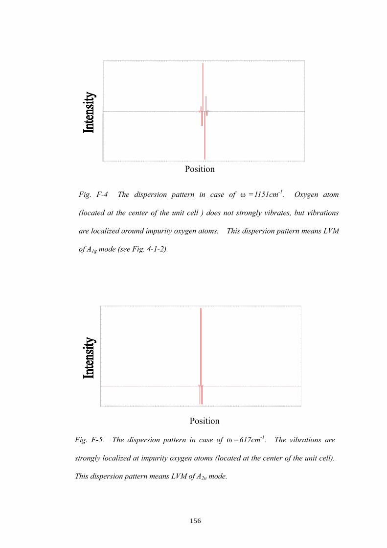
156
Fig. F-5. The dispersion pattern in case of ω =617cm-1. The vibrations are
strongly localized at impurity oxygen atoms (located at the center of the unit cell).
This dispersion pattern means LVM of A2u mode.
Fig. F-4 The dispersion pattern in case of ω =1151cm-1. Oxygen atom
(located at the center of the unit cell ) does not strongly vibrates, but vibrations
are localized around impurity oxygen atoms. This dispersion pattern means LVM
of A1g mode (see Fig. 4-1-2).
Position
Position

157
Appendix G: Calculation for vibration energies of oxygen in silicon crystal with
a liner chain model of 20 atoms.
K=113.33064;
k=479.18;
M1=4.64951*10^-26; M2=4.64951*10^-26; M3=4.64951*10^-26; M4=4.64951*10^-26; M5=4.64951*10^-26;
M6=4.64951*10^-26; M7=4.64951*10^-26; M8=4.64951*10^-26;
M9=4.64951*10^-26; M10=2.65686*10^-26; M11=4.64951*10^-26; M12=4.64951*10^-26;
M13=4.64951*10^-26; M14=4.64951*10^-26; M15=4.64951*10^-26; M16=4.64951*10^-26;
M17=4.64951*10^-26; M18=4.64951*10^-26; M19=4.64951*10^-26; M20=4.64951*10^-26;
tensol:=Eigensystem[
2K/Sqrt[M1]/Sqrt[M1], -K/Sqrt[M1]/Sqrt[M2], 0, 0, 0, 0, 0, 0, 0, 0, 0, 0, 0, 0, 0, 0, 0, 0, 0, 2K/Sqrt[M20]/Sqrt[M20],
-K/Sqrt[M2]/Sqrt[M1], 2K/Sqrt[M2]/Sqrt[M2], -K/Sqrt[M2]/Sqrt[M3], 0, 0, 0, 0, 0, 0, 0, 0, 0, 0, 0, 0, 0, 0, 0, 0, 0,
0, -K/Sqrt[M3]/Sqrt[M2], 2K/Sqrt[M3]/Sqrt[M3], -K/Sqrt[M3]/Sqrt[M4], 0, 0, 0, 0, 0, 0, 0, 0, 0, 0, 0, 0, 0, 0, 0, 0,
0, 0, -K/Sqrt[M4]/Sqrt[M3], 2K/Sqrt[M4]/Sqrt[M4], -K/Sqrt[M4]/Sqrt[M5], 0, 0, 0, 0, 0, 0, 0, 0, 0, 0, 0, 0, 0, 0, 0,
0, 0, 0, -K/Sqrt[M5]/Sqrt[M4], 2K/Sqrt[M5]/Sqrt[M5], -K/Sqrt[M5]/Sqrt[M6], 0, 0, 0, 0, 0, 0, 0, 0, 0, 0, 0, 0, 0, 0,
0, 0, 0, 0, -K/Sqrt[M6]/Sqrt[M5], 2K/Sqrt[M6]/Sqrt[M6], -K/Sqrt[M6]/Sqrt[M7], 0, 0, 0, 0, 0, 0, 0, 0, 0, 0, 0, 0, 0,
0, 0, 0, 0, 0, -K/Sqrt[M7]/Sqrt[M6], 2K/Sqrt[M7]/Sqrt[M7], -K/Sqrt[M7]/Sqrt[M8], 0, 0, 0, 0, 0, 0, 0, 0, 0, 0, 0, 0,
0, 0, 0, 0, 0, 0, -K/Sqrt[M8]/Sqrt[M7], 2K/Sqrt[M8]/Sqrt[M8], -K/Sqrt[M8]/Sqrt[M9], 0, 0, 0, 0, 0, 0, 0, 0, 0, 0, 0,
0, 0, 0, 0, 0, 0, 0, -K/Sqrt[M9]/Sqrt[M8], (K+k)/Sqrt[M9]/Sqrt[M9],-k/Sqrt[M9]/Sqrt[M10], 0, 0, 0, 0, 0, 0, 0, 0, 0, 0,
0, 0, 0, 0, 0, 0, 0, 0, -k/Sqrt[M10]/Sqrt[M9], 2k/Sqrt[M10]/Sqrt[M10], -k/Sqrt[M10]/Sqrt[M11], 0, 0, 0, 0, 0, 0, 0, 0, 0,
0, 0, 0, 0, 0, 0, 0, 0, 0, -k/Sqrt[M11]/Sqrt[M10], (k+K)/Sqrt[M11]/Sqrt[M11], -K/Sqrt[M11]/Sqrt[M12], 0, 0, 0, 0, 0, 0, 0, 0,
0, 0, 0, 0, 0, 0, 0, 0, 0, 0, -K/Sqrt[M12]/Sqrt[M11], 2K/Sqrt[M12]/Sqrt[M12], -K/Sqrt[M12]/Sqrt[M13], 0, 0, 0, 0, 0, 0, 0,
0, 0, 0, 0, 0, 0, 0, 0, 0, 0, 0, -K/Sqrt[M13]/Sqrt[M12], 2K/Sqrt[M13]/Sqrt[M13], -K/Sqrt[M13]/Sqrt[M14], 0, 0, 0, 0, 0, 0,
0, 0, 0, 0, 0, 0, 0, 0, 0, 0, 0, 0, -K/Sqrt[M14]/Sqrt[M13], 2K/Sqrt[M14]/Sqrt[M14], -K/Sqrt[M14]/Sqrt[M15], 0, 0, 0, 0, 0,
(A programming code for Mathmatica)

158
0, 0, 0, 0, 0, 0, 0, 0, 0, 0, 0, 0, 0, -K/Sqrt[M15]/Sqrt[M14], 2K/Sqrt[M15]/Sqrt[M15], -K/Sqrt[M15]/Sqrt[M16], 0, 0, 0, 0,
0, 0, 0, 0, 0, 0, 0, 0, 0, 0, 0, 0, 0, 0, -K/Sqrt[M16]/Sqrt[M15], 2K/Sqrt[M16]/Sqrt[M16], -K/Sqrt[M16]/Sqrt[M17], 0, 0, 0,
0, 0, 0, 0, 0, 0, 0, 0, 0, 0, 0, 0, 0, 0, 0, -K/Sqrt[M17]/Sqrt[M16], 2K/Sqrt[M17]/Sqrt[M17], -K/Sqrt[M17]/Sqrt[M18], 0, 0,
0, 0, 0, 0, 0, 0, 0, 0, 0, 0, 0, 0, 0, 0, 0, 0, -K/Sqrt[M18]/Sqrt[M17], 2K/Sqrt[M18]/Sqrt[M18], -K/Sqrt[M18]/Sqrt[M19], 0,
0, 0, 0, 0, 0, 0, 0, 0, 0, 0, 0, 0, 0, 0, 0, 0, 0, -K/Sqrt[M19]/Sqrt[M18], 2K/Sqrt[M19]/Sqrt[M19], -K/Sqrt[M19]/Sqrt[M20],
2K/Sqrt[M1]/Sqrt[M1], 0, 0, 0, 0, 0, 0, 0, 0, 0, 0, 0, 0, 0, 0, 0, 0, 0, -K/Sqrt[M20]/Sqrt[M19], 2K/Sqrt[M20]/Sqrt[M20]]
wavenumber=Sqrt[tensol[[1,1]]]*5.3129*10^-12,Sqrt[tensol[[1,2]]]*5.3129*10^-12,Sqrt[tensol[[1,3]]]*5.3129*10^-12,Sqrt[t
ensol[[1,4]]]*5.3129*10^-12,Sqrt[tensol[[1,5]]]*5.3129*10^-12,Sqrt[tensol[[1,6]]]*5.3129*10^-12,Sqrt[tensol[[1,7]]]*5.3129*
10^-12,Sqrt[tensol[[1,8]]]*5.3129*10^-12,Sqrt[tensol[[1,9]]]*5.3129*10^-12,Sqrt[tensol[[1,10]]]*5.3129*10^-12,Sqrt[tensol[[
1,11]]]*5.3129*10^-12,Sqrt[tensol[[1,12]]]*5.3129*10^-12,Sqrt[tensol[[1,13]]]*5.3129*10^-12,Sqrt[tensol[[1,14]]]*5.3129*1
0^-12,Sqrt[tensol[[1,15]]]*5.3129*10^-12,Sqrt[tensol[[1,16]]]*5.3129*10^-12,Sqrt[tensol[[1,17]]]*5.3129*10^-12,Sqrt[tensol[
[1,18]]]*5.3129*10^-12,Sqrt[tensol[[1,19]]]*5.3129*10^-12,Sqrt[tensol[[1,20]]]*5.3129*10^-12

159
Appendix H: Calculation for vibration energy of oxygen doped silicon crystal
with a three-dimensional nine-atom molecule model
We explain a three-dimensional calculation of LVM assuming a molecule
shown in Fig. H-1. We label these atoms from 1 to 9 in order to explain our
calculation easily. The atoms numbered 1 to 6 are 2nd nearest-neighboring Si atoms
in Fig. H-1. The atoms named as 7 and 8 are 1st nearest-neighboring Si atoms, and
the atom named as 9 is an interstitial O atom. The force constant between Si atoms
is labeled K, and between Si and O atoms is k. In order to simplify the calculation,
the interstitial O atom and its first nearest Si atoms vibrate only along 〈111〉
direction. Under this assumption, we can obtain the three-dimensional vibrations
of each atom by two-dimensional calculations.
Fig. H-1. Interstitial Oxygen (red one) and Silicon atoms (gray ones). Second
nearest Si atoms are labeled as 1 to 6. First nearest Si atoms are 7 and 8.
Interstitial O atom is 9.
1 2 3
4 5
6
7
8
9
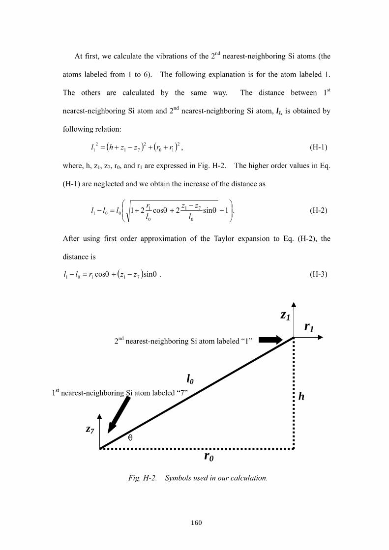
160
At first, we calculate the vibrations of the 2nd nearest-neighboring Si atoms (the
atoms labeled from 1 to 6). The following explanation is for the atom labeled 1.
The others are calculated by the same way. The distance between 1st
nearest-neighboring Si atom and 2nd nearest-neighboring Si atom, l1, is obtained by
following relation:
( ) ( )210
271
21 rrzzhl ++−+= , (H-1)
where, h, z1, z7, r0, and r1 are expressed in Fig. H-2. The higher order values in Eq.
(H-1) are neglected and we obtain the increase of the distance as
−
−++=− 1sin2cos21
0
71
0
1001 θθ
lzz
lrlll . (H-2)
After using first order approximation of the Taylor expansion to Eq. (H-2), the
distance is
( ) θθ sincos 71101 zzrll −+=− . (H-3)
θ
l0
h
z7
z1 r1
r0
2nd nearest-neighboring Si atom labeled “1”
1st nearest-neighboring Si atom labeled “7”
Fig. H-2. Symbols used in our calculation.
161
Now we obtain two motion equations that are perpendicular and parallel to 〈111〉
direction of Si crystal as follows:
( ) ( ) θθθ
θθθ
cossinsin
cossincos
12
7111
217111
rzzKzm
rzzKrm
+−−=
+−−=
&&
&&. (H-4)
We assume a harmonic vibration of each atom,
( )( )( )tiZz
tiZztiRr
ωωω
expexpexp
77
11
11
===
(H-5)
Then, Eq. (H-5) is expressed as
( ) ( ) θθθω
θθθω
cossinsin
cossincos
12
7112
1
21711
21
RZZKZm
RZZKRm
+−=
+−= (H-6)
The atoms labeled 7, 8 and 9 are also expressed as
(H-7)
Namely, the calculation we should solve is obtained as following from Eq. (H-6) and
(H-7),
( ) ( ) ( )( ) ( ) ( )( )9879
29
6542
83218982
8
3212
73217972
7
2
sincossin3
sincossin3
ZZZkZm
RRRKZZZZCZZkZm
RRRKZZZZCZZkZm
−−−=
++−−++−+=
++−−++−−−=
ω
θθθω
θθθω
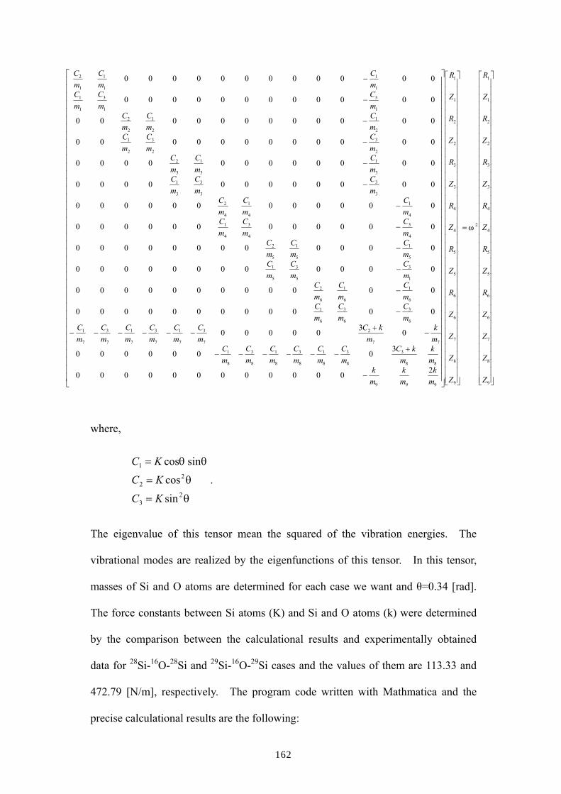
162
where,
θ
θ
θθ
23
22
1
sin
cossincos
KC
KC
KC
=
=
=
.
The eigenvalue of this tensor mean the squared of the vibration energies. The
vibrational modes are realized by the eigenfunctions of this tensor. In this tensor,
masses of Si and O atoms are determined for each case we want and θ=0.34 [rad].
The force constants between Si atoms (K) and Si and O atoms (k) were determined
by the comparison between the calculational results and experimentally obtained
data for 28Si-16O-28Si and 29Si-16O-29Si cases and the values of them are 113.33 and
472.79 [N/m], respectively. The program code written with Mathmatica and the
precise calculational results are the following:
=
−
+−−−−−−
−+
−−−−−−
−
−
−
−
−
−
−
−
−
−
−
−
9
8
7
6
6
5
5
4
4
3
3
2
2
1
1
2
9
8
7
6
6
5
5
4
4
3
3
2
2
1
1
999
88
3
8
3
8
1
8
3
8
1
8
3
8
1
77
2
7
3
7
1
7
3
7
1
7
3
7
1
6
3
6
3
6
1
6
1
6
1
6
2
1
3
5
3
5
1
5
1
5
1
5
2
4
3
4
3
4
1
4
1
4
1
4
2
3
3
3
3
3
1
3
1
3
1
3
2
2
3
2
3
2
1
2
1
2
1
2
2
1
3
1
3
1
1
1
1
1
1
1
2
2000000000000
30000000
0300000
000000000000
000000000000
000000000000
000000000000
000000000000
000000000000
000000000000
000000000000
000000000000
000000000000
000000000000
000000000000
Z
Z
Z
Z
R
Z
R
Z
R
Z
R
Z
R
Z
R
Z
Z
Z
Z
R
Z
R
Z
R
Z
R
Z
R
Z
R
mk
mk
mk
mk
mkC
mC
mC
mC
mC
mC
mC
mk
mkC
mC
mC
mC
mC
mC
mC
mC
mC
mC
mC
mC
mC
mC
mC
mC
mC
mC
mC
mC
mC
mC
mC
mC
mC
mC
mC
mC
mC
mC
mC
mC
mC
mC
mC
mC
mC
mC
mC
mC
mC
mC
mC
ω

163
OldK= 113.33;Oldkk= 679.18;θ = 0.3374;M= 1.6605402×10⁻²⁷;Ans1= 1000;Ans2= 1000;Sub1= 1000000000;Sub2= 30000;
ForAi= 1, i< 1000, i++,S= 1;K= OldK+ HRandom@D − 0.5L∗OldKêSqrt@iD;k= Oldkk+ HRandom@D − 0.5L∗OldkkêSqrt@iD;c1=
1è 2KCos@θD Sin@θD;
c2=1è 2
KCos@θD Cos@θD;
c3=1è 2
KSin@θD Sin@θD;
m1= 28 M;m2= 28 M;m3= 28 M;m4= 28 M;m5= 28 M;m6= 28 M;m7= 28 M;m8= 28 M;m9= 16 M;wavenumber1= 1151.5;tensol1= Eigensystem@88c2ê m1, c1ê m1, 0, 0, 0, 0, 0, 0, 0, 0, 0, 0, −c1ê m1, 0, 0<,8c1ê m1, c3ê m1, 0, 0, 0, 0, 0, 0, 0, 0, 0, 0, −c3ê m1, 0, 0<,80, 0, c2ê m2, c1ê m2, 0, 0, 0, 0, 0, 0, 0, 0, −c1ê m2, 0, 0<,80, 0, c1ê m2, c3ê m2, 0, 0, 0, 0, 0, 0, 0, 0, −c3ê m2, 0, 0<,80, 0, 0, 0, c2ê m3, c1ê m3, 0, 0, 0, 0, 0, 0, −c1ê m3, 0, 0<,80, 0, 0, 0, c1ê m3, c3ê m3, 0, 0, 0, 0, 0, 0, −c3ê m3, 0, 0<,80, 0, 0, 0, 0, 0, c2ê m4, c1ê m4, 0, 0, 0, 0, 0, −c1ê m4, 0<,80, 0, 0, 0, 0, 0, c1ê m4, c3ê m4, 0, 0, 0, 0, 0, −c3ê m4, 0<,80, 0, 0, 0, 0, 0, 0, 0, c2ê m5, c1ê m5, 0, 0, 0, −c1ê m5, 0<,80, 0, 0, 0, 0, 0, 0, 0, c1ê m5, c3ê m5, 0, 0, 0, −c3ê m5, 0<,80, 0, 0, 0, 0, 0, 0, 0, 0, 0, c2ê m6, c1ê m6, 0, −c1ê m6, 0<,80, 0, 0, 0, 0, 0, 0, 0, 0, 0, c1ê m6, c3ê m6, 0, −c3ê m6, 0<,8−c1ê m7, −c3ê m7, −c1ê m7, −c3ê m7, −c1ê m7, −c3ê m7, 0,
0, 0, 0, 0, 0, 3c3ê m7+kê m7, 0, −kê m7<,80, 0, 0, 0, 0, 0, −c1ê m8, −c3ê m8, −c1ê m8, −c3ê m8,−c1ê m8, −c3ê m8, 0, 3c3ê m8+ kê m8, kê m8<,

164
80, 0, 0, 0, 0, 0, 0, 0, 0, 0, 0, 0, −kê m9, kê m9, 2kê m9<<D;
mm1= 29 M;mm2= 29 M;mm3= 29 M;mm4= 29 M;mm5= 29 M;mm6= 29 M;mm7= 29 M;mm8= 29 M;mm9= 16 M;
wavenumber2= 1147.5;tensol2= Eigensystem@88c2ê mm1, c1ê mm1, 0, 0, 0, 0, 0, 0, 0, 0, 0, 0, −c1ê mm1, 0, 0<,8c1ê mm1, c3ê mm1, 0, 0, 0, 0, 0, 0, 0, 0, 0, 0, −c3ê mm1, 0, 0<,80, 0, c2ê mm2, c1ê mm2, 0, 0, 0, 0, 0, 0, 0, 0, −c1ê mm2, 0, 0<,80, 0, c1ê mm2, c3ê mm2, 0, 0, 0, 0, 0, 0, 0, 0, −c3ê mm2, 0, 0<,80, 0, 0, 0, c2ê mm3, c1ê mm3, 0, 0, 0, 0, 0, 0, −c1ê mm3, 0, 0<,80, 0, 0, 0, c1ê mm3, c3ê mm3, 0, 0, 0, 0, 0, 0, −c3ê mm3, 0, 0<,80, 0, 0, 0, 0, 0, c2ê mm4, c1ê mm4, 0, 0, 0, 0, 0, −c1ê mm4, 0<,80, 0, 0, 0, 0, 0, c1ê mm4, c3ê mm4, 0, 0, 0, 0, 0, −c3ê mm4, 0<,80, 0, 0, 0, 0, 0, 0, 0, c2ê mm5, c1ê mm5, 0, 0, 0, −c1ê mm5, 0<,80, 0, 0, 0, 0, 0, 0, 0, c1ê mm5, c3ê mm5, 0, 0, 0, −c3ê mm5, 0<,80, 0, 0, 0, 0, 0, 0, 0, 0, 0, c2ê mm6, c1ê mm6, 0, −c1ê mm6, 0<,80, 0, 0, 0, 0, 0, 0, 0, 0, 0, c1ê mm6, c1ê mm6, 0, −c3ê mm6, 0<,8−c1ê mm7, −c3ê mm7, −c1ê mm7, −c3ê mm7, −c1ê mm7, −c3ê mm7,
0, 0, 0, 0, 0, 0, 3c3ê mm7+ kê mm7, 0, −kê mm7<,80, 0, 0, 0, 0, 0, −c1ê mm8, −c3ê mm8, −c1ê mm8, −c3ê mm8,−c1ê mm8, −c3ê mm8, 0, 3c3ê mm8+ kê mm8, kê mm8<,80, 0, 0, 0, 0, 0, 0, 0, 0, 0, 0, 0, −kê mm9, kê mm9, 2kê mm9<<D;
SS1= Sub1;SS2= Sub2;
If@Abs@Hwavenumber1− Sqrt@tensol1@@1, 1DDD∗ 5.3129∗10^−12LD < SS1 &&Abs@Hwavenumber2− Sqrt@tensol2@@1, 1DDD∗ 5.3129∗10^−12LD < SS2,
Ans1= Sqrt@tensol1@@1, 1DDD∗5.3129∗10^−12D;
If@Abs@Hwavenumber1− Sqrt@tensol1@@1, 1DDD∗ 5.3129∗10^−12LD < SS1 &&Abs@Hwavenumber2− Sqrt@tensol2@@1, 1DDD∗ 5.3129∗10^−12LD < SS2,
Ans2= Sqrt@tensol2@@1, 1DDD∗5.3129∗10^−12D;
If@Abs@Hwavenumber1− Sqrt@tensol1@@1, 1DDD∗ 5.3129∗10^−12LD < SS1 &&Abs@Hwavenumber2− Sqrt@tensol2@@1, 1DDD∗ 5.3129∗10^−12LD < SS2,
Sub1= Abs@Hwavenumber1− Sqrt@tensol1@@1, 1DDD∗ 5.3129∗10^−12LDD;
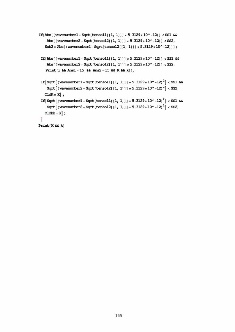
165
If@Abs@Hwavenumber1− Sqrt@tensol1@@1, 1DDD∗ 5.3129∗10^−12LD < SS1 &&Abs@Hwavenumber2− Sqrt@tensol2@@1, 1DDD∗ 5.3129∗10^−12LD < SS2,
Sub2= Abs@Hwavenumber2− Sqrt@tensol2@@1, 1DDD∗ 5.3129∗10^−12LDD;
If@Abs@Hwavenumber1− Sqrt@tensol1@@1, 1DDD∗ 5.3129∗10^−12LD < SS1 &&Abs@Hwavenumber2− Sqrt@tensol2@@1, 1DDD∗ 5.3129∗10^−12LD < SS2,
Print@i && Ans1− 15 && Ans2− 15 && K && kDD;
IfASqrtAHwavenumber1− Sqrt@tensol1@@1, 1DDD∗ 5.3129∗10^−12L2E < SS1 &&SqrtAHwavenumber2− Sqrt@tensol2@@1, 1DDD∗ 5.3129∗10^−12L2E < SS2,
OldK= KE ;IfASqrtAHwavenumber1− Sqrt@tensol1@@1, 1DDD∗ 5.3129∗10^−12L2E < SS1 &&
SqrtAHwavenumber2− Sqrt@tensol2@@1, 1DDD∗ 5.3129∗10^−12L2E < SS2,Oldkk= kE;E
Print@K && kD

166
Acknowledgements
Without the guidance, encouragement and generous support of Professor
Kohei M. Itoh, none of the present work would have been possible. I am grateful
to have the continuous benefit of his expertise in the physics and materials science of
semiconductors.
Many professors have substantially aided my research. I am grateful to
Professor Jun-ichiro Muto for his expert advices on electric materials in general.
Novel germanium crystals we investigated were provided by Professor Eugen E.
Haller. He also taught me the importance of studying defects in semiconductors.
I extend my thanks to Dr. Hiroshi Yamada-Kaneta, without his expertise in oxygen
in silicon, the study of the local vibrational modes of oxygen in silicon crystal
described in this thesis would not habe been completed. Professor Hyunjung Kim
taught me how to push the limit of Fourier transform spectroscopy of
semiconductors. I would like to thank Professor Eiji Ohta and Professor Shuichi
Nose for their critical reading of this thesis. Toshimichi Yamada and Eisuke Abe
have also contributed to improve my English writing.