Effects of Per-Vehicle Entrance Fees on U.S. National Park

Effects of Per-Vehicle Entrance Fees on U.S. National Park Visitation Rates

Seth Factor

Abstract

This study tested the hypothesis that increases in per-vehicle entrance fees at United

States National Parks between the years 1996 and 2006 resulted in reduced numbers of

park visitors. Analysis proceeded in three stages: (1) annual visitor numbers and entrance

fees were plotted together over the 11 year period; (2) a difference-in-difference analysis

was performed, comparing visitor trends for clusters of similar parks from the year before

to the year after that in which fees were increased; and (3) the natural log of yearly visitor

count was regressed on the natural log of fees in an attempt to quantify the elasticity

relationship between the two variables. The analysis did not find a clear relationship

between per-vehicle entrance fees and visitation rates. However, the possibility remains

that such a relationship exists, at least for some parks.

I. Introduction

National parks around the country have been steadily raising entrance fees since

Congress expanded their authority to do so in 1996. Predictably, the increased cost to the

public has sparked some controversy; opponents of the fee increases are concerned that

higher prices will exclude lower income citizens from national parks, and discourage use

by other citizens with marginal preferences for visiting national parks. To assess the

validity of these claims, I analyzed the question: Do per-vehicle entrance fees affect

yearly visitation rates of U.S. National Parks? Analysis proceeded in three stages;

(1) visitor number and fee data were plotted over time and examined visually; (2) a

2

difference-in-difference analysis was conducted comparing visitor trends of clusters of

similar parks from the year before until the year after fees were increased; and (3) the

natural log of yearly visitor count was regressed on the natural log of fees in an attempt to

quantify the elasticity relationship between the two variables.

II. Background

In 1996, Congress authorized the Recreation Fee Demonstration Program. Under this

program, four government agencies – the National Park Service, the Fish and Wildlife

Service, the Bureau of Land Management, and the Forest Service – were authorized to

establish, charge, and collect fees, and required to spend 80 percent of the revenue at the

site at which it was collected. Originally scheduled to expire in December 2005,

Congress extended this authority for an additional ten years as part of the 2005 Omnibus

Appropriations Bill, under the new Federal Lands Recreation Act.

Each year from 1997 to 2006, the Department of the Interior (DOI) submitted reports to

congress detailing the status of the program.1 From 1996 to 2001, the number of

National Park Service (NPS) sites in the fee demonstration program was set to 100 (there

are currently 391 sites in the NPS system), allowing a consistent comparison of visitation

rates for sites included and those not included in the program (Figure 1).

1 Department of Interior, The Recreation Fee Program, http://www.doi.gov/initiatives/recreation_feeprogram.html, (July, 2007).

3

NPS Recreation Visits (millions)

0

20

40

60

80

100

120

140

160

180

1994 1995 1996 1997 1998 1999 2000 2001

Year

NPS Fee demo sites All other NPS sites

Figure 1. Comparison of visitation rates at demo and non-demo NPS sites.

In 2002, the number of sites in the program increase to 236, preventing further simple

year-to-year comparisons. At that point, DOI reports began limiting their discussion to

the general overall trends in visitation at fee sites, foregoing a comparison with non-fee

sites. In the final report for the program, discussion of visitation rates is limited to one

section in the executive summary. That section reads:

Aggregate visitation to recreation sites participating in the Fee Demo

Program continues to be unaffected in any significant way by fees (see

Table 1). Total visitation to fee and non-fee sites has remained relatively

constant over the last five years, averaging approximately 370 million

visitors per year. 2

However, the data referenced in Table 1 (reproduced here in Appendix A) are insufficient

to allow DOI to make such a determination of no-effect. One limitation is that NPS sites

2 Department of the Interior, FY 2004 Recreation Fee Demonstration Program Summary: Visitation, Revenue, Cost, and Obligation Information, 2004. (p. 2). http://www.doi.gov/initiatives/FY_2004_Accomplishments_financial_information.pdf. (July, 2007).

4

were not randomly selected for inclusion in the program. As a result, sites included in the

program were systematically different from those that were not; almost all of the sites

included in the original 100 were already charging fees before the program went into

effect, whereas none of the non-demonstration sites was.

Furthermore, by aggregating all recreation sites, the DOI analysis obscures any

differences in trends that might exist between the visitation rates of demonstration and

non-demonstration sites. It allows for the possibility that visitor increases at non-

demonstration sites could be obscuring visitor decreases at demonstration sites.

Finally, the sites lumped together by DOI as “fee demonstration sites” vary

fundamentally by type. DOI’s reports disaggregate sites only to the level of the

managing agency, leaving grouped, for example, national parks, national historic sites

and national recreation areas. However, it seems reasonable to think that these types of

sites might be affected by fee changes differently.

Several other studies have searched for a relationship between visitor numbers and

entrance fees for U.S. recreation areas. Using a chi square test for statistical significance,

Becker, et al, concluded that the reduction in visitation at South Carolina State Parks

between 1980 and 1982 was not associated with the introduction of entrance fees in

1982.3 Analyzing a mail survey of New Hampshire and Vermont households, More and

Stevens concluded that user fees may reduce participation in resource-based recreation by

3 R.H. Becker, Deborah Berrier, and G.D. Barker, “Entrance Fees and Visitation Levels,” Journal of Park and Recreation Adminstration. 3, no 1 (1985).

5

those earning less than $30,000 per year.4 Through factor analysis of data collected from

a national phone survey of 3.515 people, Ostergen, et al, concluded that entrance fees do

not represent a barrier to visitation of National Park Service units.5 Finally, Ngure and

Chapman applied ordinary least squares regression to National Park visitation and fee

data for the years 1993, 1994 and 1996. 6 While they were unable to demonstrate an

effect of fee levels during those periods, these authors speculated that “much higher fees

would significantly affect park visitation levels.”

III. Data

This analysis was performed with geospatial and tabular data obtained from a variety of

sources, as described below. Summary statistics for the tabular data appear in

Appendix B.

Parks

In order to analyze a more homogeneous sample than that which the Department of

Interior analyzed, the data set was limited to include only National Parks, and only those

that were part of the fee demonstration program.

Sequoia and Kings Canyon National Parks were excluded because at some point after

1996 the Park Service began tabulating visitor numbers for the two parks together. Dry

Tortugas, Carlsbad Canyon, and Guadalupe Mountains National Parks were excluded

4 Thomas More and Thomas Stevens,“Do User Fees Exclude Low-income People from Resource-based Recreation?” Journal of Leisure Research 32, no. 3 (2000). 5 David Ostergren, Frederic I. Solop, and Kristi K. Hagen, “National Park Service Fees: Value for the Money or a Barrier to Visitation?” Journal of Park and Recreation Administration 23, no 1 (2005). 6 Njorge Ngure and Duane Chapman, “Demand for Visitation to U.S. National Park Areas: Entrance Fees and Individual Area Attributes,” Working Paper of the Dept. of Agricultural, Resource, and Managerial Economics, Cornell University (1999).

6

from the analysis because they do not charge per-vehicle entrance fees. Table 1 lists the

remaining 29 national parks that were included in this analysis, and the fees they charged

during the period under investigation.

National Park 1996 1997 1998 1999 2000 2001 2002 2003 2004 2005 2006

Acadia 6.42 6.28 12.37 12.1 11.71 11.38 11.21 10.96 21.34 20.65 20.00

Arches 0 0 0 0 11.71 11.38 11.21 10.96 10.67 10.32 10.00

Badlands 6.42 6.28 12.37 12.1 11.71 11.38 11.21 10.96 10.67 15.48 15.00

Big Bend 6.42 6.28 12.37 12.1 11.71 11.38 11.21 16.43 16.01 15.48 15.00

Black Canyon of

the Gunnison 5.14 5.02 8.66 8.47 8.2 7.97 7.84 7.67 8.54 8.26 8.00

Bryce Canyon 6.42 6.28 12.37 12.1 23.41 22.77 22.41 21.91 21.34 20.65 20.00

Canyonlands 5.14 5.02 12.37 12.1 11.71 11.38 11.21 10.96 10.67 10.32 10.00

Capitol Reef 0 0 0 0 4.68 5.69 5.6 5.48 5.34 5.16 5.00

Crater Lake 6.42 6.28 12.37 12.1 11.71 11.38 11.21 10.96 10.67 10.32 10.00

Death Valley 6.42 6.28 12.37 12.1 11.71 11.38 11.21 10.96 10.67 10.32 20.00

Denali 6.42 6.28 12.37 12.1 11.71 11.38 11.21 10.96 21.34 20.65 20.00

Everglades 6.42 6.28 12.37 12.1 11.71 11.38 11.21 10.96 10.67 10.32 10.00

Glacier 0 0 0 0 11.71 11.38 11.21 10.96 21.34 20.65 25.00

Grand Canyon 12.85 12.56 24.74 24.2 23.41 22.77 22.41 21.91 21.34 20.65 25.00

Grand Teton 12.85 12.56 24.74 24.2 23.41 22.77 22.41 21.91 21.34 20.65 25.00

Haleakala 5.14 5.02 12.37 12.1 11.71 11.38 11.21 10.96 10.67 10.32 10.00

Hawaii Volcanoes 6.42 6.28 12.37 12.1 11.71 11.38 11.21 10.96 10.67 10.32 10.00

Joshua Tree 6.42 6.28 12.37 12.1 11.71 11.38 11.21 10.96 10.67 10.32 15.00

Lassen Volcanic 6.42 6.28 12.37 12.1 11.71 11.38 11.21 10.96 10.67 10.32 10.00

Mesa Verde 6.42 6.28 12.37 12.1 11.71 11.38 11.21 10.96 10.67 10.32 10.00

Mount Rainier 6.42 6.28 12.37 12.1 11.71 11.38 11.21 10.96 10.67 10.32 15.00

Olympic 6.42 6.28 12.37 12.1 11.71 11.38 11.21 10.96 10.67 10.32 15.00

Petrified Forest 6.42 6.28 12.37 12.1 11.71 11.38 11.21 10.96 10.67 10.32 10.00

Rocky Mountain 6.42 6.28 12.37 12.1 17.56 17.08 16.81 16.43 16.01 20.65 20.00

Theodore Roosevelt 5.14 5.02 12.37 12.1 11.71 11.38 11.21 10.96 10.67 10.32 10.00

Yellowstone 12.85 12.56 24.74 24.2 23.41 22.77 22.41 21.91 21.34 20.65 25.00

Yosemite 6.42 6.28 24.74 24.2 23.41 22.77 22.41 21.91 21.34 20.65 20.00

Zion 6.42 6.28 12.37 12.1 23.41 22.77 22.41 21.91 21.34 20.65 20.00

Table 1. Fees of national parks included in the sample (constant 2006 dollars).

Visitation data

The dependent variable in this analysis is yearly visitation rate, defined as number of

recreation visitors per year. These data, spanning from 1996 to 2006, were obtained

7

from the National Park Service Public Use Statistics Office ([Butch Street], personal

communication), and were generated from park gate records. While this variable appears

to be valid, NPS reports indicate occasional failures of vehicle counters at park gates

which result in underreporting of visitor numbers.

Fee data

Per-vehicle fee is the primary independent variable used in the analysis. Entrance fees

from 1996 to 2006 for all parks in the demonstration program were obtained from a Fee

Management Program analyst with the National Park Service. Data were adjusted for

inflation using the Consumer Price Index and reported in constant 2006 dollars.

Other independent variables

Average yearly unemployment rates, as reported by the Current Population Survey, were

obtained from the Bureau of Labor Statistics. Average yearly gasoline prices were

obtained from the Energy Information Administration. These prices were adjusted for

inflation using the Consumer Price Index and reported in constant 2006 cents. Two

geospatial data sets were downloaded from the National Atlas website7: United States

county boundaries for the year 2000, and population data from the year 2000 Decennial

Census (U.S. Census Bureau, 2000). Two other geospatial data sets were downloaded

from the National Park Service Data Store website8: National park boundaries, and

national park visitor services locations.

7 National Park Service Data Store website. http://science.nature.nps.gov/nrdata/. (July, 2007). 8 Ibid.

8

IV. Analytical approach

Analysis was performed in three stages. First, the data were plotted graphically and

checked for (1) problems stemming from inconsistent collection methods, (2) consistency

in trends over time among parks, and (3) any immediate indications of a relationship

between fee levels and visitor numbers. Second, parks were clustered into small

homogenous groups on which difference-in-difference analyses were performed; parks

that raised fees were compared with those that did not. Finally, the natural log of visitor

numbers was regressed on the natural log of fees in a series of progressively complex

regressions, in an attempt to determine the precise price elasticity of demand for park

visitation.

A. Data checking and preliminary assessment

Yearly visitation rates and per-vehicle entrance fees were graphed for each park from

1996 to 2006 (see Appendix C), as was the combined visitation rate for all parks in the

sample over this same time period (Figure 2). The graphs served three purposes: First,

they allowed me to examine the data for any inconsistencies which might have arisen

from changes in recording methods. Second, viewing the degree to which visitation rates

for different parks trended together over time allowed me to determine how well parks

could serve as controls for each other in later regression analyses. Finally, the graphs

allowed me to look for any immediately obvious effects of fee changes on visitation

rates.

9

Visitor rates, all parks with fees (1996-2006)

37000000

38000000

39000000

40000000

41000000

42000000

43000000

44000000

45000000

46000000

1996 1997 1998 1999 2000 2001 2002 2003 2004 2005 2006

Year

Nu

mb

er

of

vis

ito

rs

Figure 2. Visitor rates of all fee-charging parks, 1996-2007

B. Difference-in-difference analysis

The graphical analysis revealed that parks differ greatly in their visitation patterns over

time. This variation indicates that different parks are influenced by different factors, or

by the same factors at different times. In order to remove some of the bias introduced by

these differences, parks were grouped into small, homogenous clusters that were

presumed to respond similarly to all external factors. Within each cluster, visitor

numbers of parks that increased fees were then compared with those that did not. Results

were examined non-parametrically in a difference-in-difference analysis; a strong

tendency for parks that raised fees to have a more downward trend in visitor numbers

than those that did not raise fees would have been interpreted as evidence that increased

fees result in decreased visitor numbers.

10

Clustering parks

1. Estimated population within 100 km of each park visitor center

This criterion was chosen based on the rationale that difficult-to-access parks should be

less responsive to fee increases than those that are easier to access. Because entrance fees

make up such a small fraction of the overall cost of a typical visit to a remote national

park, one would expect that these fees would have little influence over a prospective

visitor’s decision of whether or not to visit.

The following steps were performed using ESRI ARC GIS 9.2 to achieve the estimation:

(a) Visitor services points were intersected with park boundaries to limit the points to

only those that fall within park boundaries.

(b) Among the visitor services points, only those with a “visitor center” attribute were

selected.

(c) 100 km buffers were drawn around each visitor center.

(d) Population census data was joined to the spatial county data using the FIPS code.

(e) The area of each county contained in each buffer was calculated.

(f) To estimate the population of each portion of each county comprising the buffers,

the areas calculated in the previous step were multiplied by the population density

of each county (this data was included with the census population data set).

Summing the results for each park resulted in an estimate of the number of people

residing within 100 km of each park visitor center.

11

(g) Parks were then segregated into four categories by applying a Jenks Natural

Breaks procedure to the resulting population distribution. Figure 3 provides a

graphical representation of the results for parks in the lower 48 states.

Figure 3. Estimated population within 100 km of National Parks in the sample.

2. Driving time to the nearest interstate highway.

Driving times from park visitor centers to nearest interstate highway were obtained using

Google Maps.9 Coordinates of park visitor centers (from the national park visitor

services data set cited above) were entered as starting locations, and the nearest interstate

highway entrance was entered as ending locations. Parks within one-half hour of

interstate highways were considered as distinct from those parks which are more distant

from highways. The assumption was that a non-trivial number of visitors to parks close

9 Google Maps. http://www.maps.google.com. (July, 2007).

12

to highways are travelers who stop for a quick and easy diversion while passing by on the

interstate to a different destination.

3. Number of visitors

Parks that differed greatly in the number of visitors they receive were placed in different

clusters.

4. Geographic location

Parks that would be expected to react similarly to similar regional conditions, or would

be expected to have similar visitor patterns due to their similar locations, were generally

and subjectively clustered together based. Clusters with strong geographic influence

included: Hawaii parks, Midwestern parks, Big Bend and Denali – the spatially isolated

parks; small Pacific coast parks; secondary Grand Canyon area parks; tertiary Grand

Canyon area parks; and southwestern Colorado parks.

5. Visual assessment of graphed year-to-year trends in visitation

All parks were indexed to 100 visitors in 1999, and graphed in preliminary clusters based

on a subjective review of the results of the preceding steps. The resulting graphs depicted

the trends in visitor numbers from year to year for each park in such a way that easy

inter-park comparisons could be made. Parks were shuffled among clusters until each

cluster contained only parks which trended relatively closely together (Table 2). See

Appendix D for the final graphs. Arrows were added to these graphs to indicate the year

and magnitude of fee increases.

13

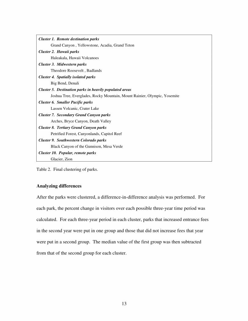
Cluster 1. Remote destination parks

Grand Canyon , Yellowstone, Acadia, Grand Teton

Cluster 2. Hawaii parks

Haleakala, Hawaii Volcanoes

Cluster 3. Midwestern parks

Theodore Roosevelt , Badlands

Cluster 4. Spatially isolated parks

Big Bend, Denali

Cluster 5. Destination parks in heavily populated areas

Joshua Tree, Everglades, Rocky Mountain, Mount Rainier, Olympic, Yosemite

Cluster 6. Smaller Pacific parks

Lassen Volcanic, Crater Lake

Cluster 7. Secondary Grand Canyon parks

Arches, Bryce Canyon, Death Valley

Cluster 8. Tertiary Grand Canyon parks

Petrified Forest, Canyonlands, Capitol Reef

Cluster 9. Southwestern Colorado parks

Black Canyon of the Gunnison, Mesa Verde

Cluster 10. Popular, remote parks

Glacier, Zion

Table 2. Final clustering of parks.

Analyzing differences

After the parks were clustered, a difference-in-difference analysis was performed. For

each park, the percent change in visitors over each possible three-year time period was

calculated. For each three-year period in each cluster, parks that increased entrance fees

in the second year were put in one group and those that did not increase fees that year

were put in a second group. The median value of the first group was then subtracted

from that of the second group for each cluster.

14

C. Regression analyses

In an attempt to determine the elasticity of the relationship between fees and visitor

numbers, regression analyses were conducted. This procedure expanded on the previous

difference-in-difference analysis by considering magnitudes of effects. The fee variable

and the visitor number variable were both log transformed so that the results could be

interpreted as the price elasticity of demand for park visitation.

The regressions were performed in a progressively complex sequence:

(a) A fixed effects regression was run, in which the natural log of visitor number was

regressed on the natural log of per-vehicle fees, yearly unemployment rates, and

the natural log of the yearly average gas prices, with dummy variables included

for each park. These park dummy variables in this case control for all differences

among parks that might affect visitor numbers. Gas prices and unemployment

rate (used here as a general indicator of the state of the U.S. economy) were

included because they are easily and accurately measured, and likely influence

national trends of park visitor numbers.

(b) Unemployment rates and gas prices from the previous regression were replaced

with year dummy variables, resulting in a full panel regression. Including year

dummy variables in this specification controlled for all factors beyond gas prices

and unemployment rates which might influence national trends in visitor

numbers, but which were omitted from the previous specification.

15

(c) Another full panel regression was run, again including dummy variables for parks

and years, but this time interacting the park dummy variables with the fee

variable. This specification considered the possibility that different parks react

differently to changes in fee levels. In particular, this specification allows for the

slope coefficient on the log fee variable to differ from park to park.

V. Results

Graphing trends in visitor numbers over time

Review of the graphs did not reveal any obvious problems with the data in terms of

inconsistencies in collection methods over time or between parks. The review also did

not reveal any consistent effect of fees on visitation rates.

Difference-in-difference

The difference-in-difference analysis produced nine negative and six positive

results (Table 3).

1997-1999

1998-2000

1999-2001

2000-2002

2001-2003

2002-2004

2003-2005

2004-2006

Cluster 1 -20.2

Cluster 2

Cluster 3 -2.0

Cluster 4 -20.7 -15.6

Cluster 5 0.8 7.2

Cluster 6 -16.6 -7.5 -7.1

Cluster 7

Cluster 8 -3.6 10.1

Cluster 9 -5.5

Cluster 10 1.6 10.5

Table 3. Net median percent change in number of visitors, parks that increased fees in middle year minus those that did not.

16

Regression analyses

The first regression suggested that increasing fees negatively influences visitor numbers.

However, when the second regression was run with year fixed effects included, that

influence was no longer observed. When the park variable was interacted with the fee

variable in the third regression, eight parks showed a significant relationship between

fees and visitor numbers (five negative and three positive).

See Appendix E for the STATA log file detailing the specifications and results of the

regressions. Tables 4 and 5 below describe the coefficients and standard errors for the

two fixed effects regressions that did not contain interaction terms. The first, which

controlled for gas prices, unemployment and park fixed effects, showed a 10 percent

increase in fees resulting in a 0.51 percent decrease in number of visitors (significant at

the 1% level). The second regression, which replaced the gas and unemployment

variables with year dummy variables, resulted in a slope coefficient on the fee variable

that was insignificant at the 5 percent level. An F-test indicated that the addition of the

10 year dummy variables produced a significant improvement in the specification (see

STATA log file for the test details).

4. Effects of per-vehicle entrance fees on national park visitation rates, 1996 to 2006

Estimated regression coefficients and standard errors

Dependent variable: Natural log of yearly visitor count

Park fixed effects included

R2 = .990 Fee (natural log) Unemployment Average yearly gas price (natural log)

Regression coefficient Standard Error

-.051a

(.019)

-.034 a

(.0086)

-.094a

(.028)

a Significant at the 1% level Note: Regression based on 303 observations

17


Estimated regression coefficients and standard errors

Dependent variable: Natural log of yearly visitor count

Park and year fixed effects included

R2 = .990

Fee (natural log)

Regression coefficient Standard Error

.013* (.0035)

* Not significant at the 5% level Note: Regression based on 303 observations

Table 6 shows the results of the third regression, in which fees and parks were interacted.

An F-test indicated that the interaction as a whole was significant (see STATA log file

for details of the test). As Acadia National Park was the omitted category in this

regression, the coefficient listed for that park represents the percent change in visitor

numbers for that park when fees are raised by one percent. The coefficients listed for the

other parks, when added to the coefficient for Acadia, represent the percent change in

number of visitors to those parks when fees are raised by one percent.


Estimated regression coefficients and standard errors Dependent variable = Natural log of yearly visitor count

Park and year fixed effects included

Parks and fees interacted

Interaction Coefficient Standard Error

Acadia (omitted category) -0.176a c 0.069

Arches -0.431 0.614

Badlands 0.113 0.110

Black Canyon of the Gunnison -0.009 0.153

Big Bend 0.400a * 0.100

Bryce Canyon 0.045* 0.081

Canyonlands 0.086 0.103

Capitol Reef -0.259 0.497

Crater Lake 0.130 0.130

Denali 0.369a * 0.088

Death Valley -0.077* 0.104

18

Everglades 0.392a 0.130

Glacier 0.382a * 0.114

Grand Canyon 0.077 0.127

Grand Tetons 0.134 0.127

Haleakala 0.156 0.103

Hawaii Volcanoes -0.007 0.130

Joshua Tree 0.364a 0.119

Lassen Volcanic 0.145 0.130

Mesa Verde -0.116* 0.130

Mount Rainier 0.126 0.119

Olympic 0.044 0.119

Petrified Forest -0.208* 0.130

Rocky Mountain 0.217b 0.088

Saguaro 0.213 0.178

Theodore Roosevelt 0.305a 0.103

Yellowstone 0.218 0.127

Yosemite 0.099 0.081

Zion 0.237a 0.081 a Significantly different from Acadia at the 1% level b Significantly different from Acadia at the 5% level * Slope is significantly different from zero at the 5% level R2 = .993 Note: Regression based on 303 observations

Table 7 lists the parks for which a significant relationship was found between fees and

visitor numbers, and the magnitude of those effects.

Park Percent change in visitor numbers from a 10% raise in fees

Petrified Forest -3.24

Mesa Verde -2.32

Death Valley -1.93

Acadia -1.76

Bryce Canyon -0.71

Denali 2.54

Glacier 2.66

Big Bend 2.84

Table 7. Parks with significant relationship between fees and visitor numbers.

19

VI. Discussion

Immediately upon graphing visitation numbers over time it became apparent that visitor

numbers at few of the parks in the sample have trended together. This fact made the

attempt to detect an overall effect of fees on visitor numbers challenging.

Grouping the parks into small clusters was a first attempt to deal with this variation

among parks. This was a difficult task, given the huge degree to which the parks vary

across many dimensions. While most of the final clusters were based on convincing

reasoning and resulted in groupings of parks which indeed trended together over time,

some of the parks proved difficult to place into groupings.

The difference-in-difference analysis produced one and a half times as many comparisons

that yielded a net negative effect than those that yielded a net positive effect. It would be

unwise to interpret these results on their own as proof of a causal relationship between

raised fees and reduced visitor numbers, given the subjectivity of the process and the

paucity of the data points. However, had the other results obtained from this analysis

shown a similar, negative effect of fees on visitor numbers, this difference-in-difference

analysis could have served to bolster the claim that a causal relationship exists.

The results of the regression analyses were inconclusive. While the first regression

showed a significant negative effect of fees on visitor numbers, the second regression

negated this result. It is likely that there are other time-related variables in addition to

fees, gas prices and national unemployment which may account for much of the

20

variability assigned to fees in the first regression. Possibilities for such variables, which

were omitted due to the difficult to impossible nature of gathering data for them, include:

the strength of the U.S. dollar on the international market, national and regional weather

patterns, and the cost of air travel.

Another problem with each of the first two regressions is that the parks vary so much in

their response to fees that we may not be able to conclude anything from a test designed

to find just one significant slope coefficient for all parks. The third regression attempted

to address this concern by interacting fees and parks, and thus allowing for the slope of

the relationship between fees and visitor numbers to differ for each park. Once again,

however, the results were contradictory and less than convincing. A possible explanation

is that employing a full panel regression including an interaction term consumes a large

amount of degrees of freedom, and thus results in a large amount of error. The upshot is

that even fairly large effects, if they existed, would be lost in the noise. Nonetheless,

with only eight significant results, and three of these showing strong positive effects, it

becomes still more difficult to make any case for a negative overall effect of fees on

visitor numbers.

It is difficult to reconcile the results of this final regression analysis with the final clusters

I chose for the difference-in-difference analysis. Contrary to expectations, the parks that

showed significant fee effects were almost entirely from distinct clusters. Two were

clustered together – Bryce Canyon and Death Valley; but if we want to believe that the

clusters were adequate, or that the regression results were legitimate, then we should in

21

this case have seen Arches – the third park in this cluster – also showing a significant

negative effect of fees. This was not the case.

As inconclusive as the results of this analysis appear, when taken as a whole they do

indicate that there is no clear, overall effect of fees on visitor numbers, at least at the level

of fees that have been charged to date. The possibility remains that fee levels do have an

effect on visitor numbers at some individual parks. However, it appears from this

analysis that to tease such an effect out of the myriad other influences on demand for park

entry would require an experiment of the type that would be impractical to perform in the

context of National Parks. Randomly assigning National Parks to control and treatment

groups and centrally determining the level of fees that each park could charge would be

politically impossible, as well as simply bad for business.

The generally inelastic relationship between National Park entrance fees and visitation

rates indicated by this analysis aligns well with economic theory. When people visit

parks they typically incur travel and lodging expenses greatly in excess of the park

entrance fees. Furthermore, ready substitutes for National Park visits simply do not exist;

the Grand Canyon and Arches National Park, for example, are unique to this world. The

results of this analysis suggest that in basing its fee policy on this economic theory, DOI

has acted wisely.

22

References

Becker, R.H., D. Berrier, and G.D. Barker. “Entrance Fees and Visitation Levels.” Journal of Park and Recreation 3, no. 1 (1985). Department of Interior, The Recreation Fee Program. http://www.doi.gov/initiatives/recreation_feeprogram.html (July, 2007). Department of the Interior, FY 2004 Recreation Fee Demonstration Program Summary: Visitation, Revenue, Cost, and Obligation Information, 2004. (p. 2). http://www.doi.gov/initiatives/FY_2004_Accomplishments_financial_information.pdf. (July, 2007). Google Maps. http://www.maps.google.com. (July, 2007). National Park Service Data Store website. http://science.nature.nps.gov/nrdata/. (July, 2007). More, T. and T. Stevens. “Do User Fees Exclude Low-income People from Resource-based Recreation?” Journal of Leisure Research 32. no. 3 (2000). Ngure, N and D. Chapman. “Demand for Visitation to U.S. National Park Areas: Entrance Fees and Individual Area Attributes.” Working Paper of the Dept. of Agricultural, Resource, and Managerial Economics, Cornell University (1999). Ostergren, D., F.I. Solop, and K.K. Hagen.“National Park Service Fees: Value for the Money or a Barrier to Visitation?” Journal of Park and Recreation Administration 23, no. 1 (2005).

23

Appendix A. Data analyzed by the Department of Interior

1994 1995 1996 1997 1998 1999 2000 2001 2002 2003 2004 2005

Fee demo sites 164.8 166.6 159.9 164.4 163.2 163.7 164.4 161.9 161.9 216.4 229.9 220.4

All other sites 101.7 103.0 105.9 110.8 123.5 123.4 122.1 123.3 123.3 56.9 35.5 56.0

NPS Total 266.5 269.6 265.8 275.2 286.7 287.1 286.5 285.2 285.2 277.3 265.4 276.5

Source: DOI FY 2004 Recreation Fee Demonstration Program Summary.

24

Appendix B. Variable descriptions and distribution of fees at U.S. National Parks

Variable Mean Standard Deviation Min Max

Per vehicle fee, $ 11.24 6.55 0 25

Yearly visitor count 1,401,864 1,130,304 160,450 4,791,668

Yearly average gas price, ¢ 178.09 38.92 132.55 261.83

Unemployment rate, % 4.97 0.62 4 6

25

Appendix C. Visitor numbers and fees from 1996 to 2006 for parks in the sample

Acadia

0

500000

1000000

1500000

2000000

2500000

3000000

1996 1997 1998 1999 2000 2001 2002 2003 2004 2005 2006

Year

Vis

ito

rs

0.00

5.00

10.00

15.00

20.00

25.00

Fee

Vis PVFee

Arches

0

100000

200000

300000

400000

500000

600000

700000

800000

900000

1000000

1996 1997 1998 1999 2000 2001 2002 2003 2004 2005 2006

0.00

5.00

10.00

15.00

20.00

25.00

Badlands

0

200000

400000

600000

800000

1000000

1200000

1996 1997 1998 1999 2000 2001 2002 2003 2004 2005 2006

0.00

5.00

10.00

15.00

20.00

25.00

26

Black Canyon of the Gunnison

0

50000

100000

150000

200000

250000

1996 1997 1998 1999 2000 2001 2002 2003 2004 2005 2006

0.00

5.00

10.00

15.00

20.00

25.00

30.00

Big Bend

0

50000

100000

150000

200000

250000

300000

350000

400000

450000

1996 1997 1998 1999 2000 2001 2002 2003 2004 2005 2006

0

5

10

15

20

25

Bryce Canyon

0

200000

400000

600000

800000

1000000

1200000

1400000

1996 1997 1998 1999 2000 2001 2002 2003 2004 2005 2006

0.00

5.00

10.00

15.00

20.00

25.00

27

Canyonlands

0

50000

100000

150000

200000

250000

300000

350000

400000

450000

500000

1996 1997 1998 1999 2000 2001 2002 2003 2004 2005 2006

0.00

5.00

10.00

15.00

20.00

25.00

Capital Reef

0

100000

200000

300000

400000

500000

600000

700000

800000

1996 1997 1998 1999 2000 2001 2002 2003 2004 2005 2006

0.00

5.00

10.00

15.00

20.00

25.00

Crater Lake

0

100000

200000

300000

400000

500000

600000

1996 1997 1998 1999 2000 2001 2002 2003 2004 2005 2006

0.00

5.00

10.00

15.00

20.00

25.00

28

Death Valley

0

200000

400000

600000

800000

1000000

1200000

1400000

1996 1997 1998 1999 2000 2001 2002 2003 2004 2005 2006

0.00

5.00

10.00

15.00

20.00

25.00

Denali

0

50000

100000

150000

200000

250000

300000

350000

400000

450000

1996 1997 1998 1999 2000 2001 2002 2003 2004 2005 2006

0

5

10

15

20

25

Everglades

0

200000

400000

600000

800000

1000000

1200000

1400000

1996 1997 1998 1999 2000 2001 2002 2003 2004 2005 2006

0.00

5.00

10.00

15.00

20.00

25.00

29

Glacier

0

500000

1000000

1500000

2000000

2500000

1996 1997 1998 1999 2000 2001 2002 2003 2004 2005 2006

0.00

5.00

10.00

15.00

20.00

25.00

Grand Canyon

3600000

3800000

4000000

4200000

4400000

4600000

4800000

5000000

1996 1997 1998 1999 2000 2001 2002 2003 2004 2005 2006

0.00

5.00

10.00

15.00

20.00

25.00

Grand Tetons

2100000

2200000

2300000

2400000

2500000

2600000

2700000

2800000

1996 1997 1998 1999 2000 2001 2002 2003 2004 2005 2006

0.00

5.00

10.00

15.00

20.00

25.00

30

Haleakala

0

500000

1000000

1500000

2000000

2500000

1996 1997 1998 1999 2000 2001 2002 2003 2004 2005 2006

0.00

5.00

10.00

15.00

20.00

25.00

Hawaii Volcanoes

0

200000

400000

600000

800000

1000000

1200000

1400000

1600000

1800000

2000000

1996 1997 1998 1999 2000 2001 2002 2003 2004 2005 2006

0.00

5.00

10.00

15.00

20.00

25.00

Joshua Tree

0

200000

400000

600000

800000

1000000

1200000

1400000

1600000

1996 1997 1998 1999 2000 2001 2002 2003 2004 2005 2006

0.00

5.00

10.00

15.00

20.00

25.00

31

Lassen

0

50000

100000

150000

200000

250000

300000

350000

400000

450000

1996 1997 1998 1999 2000 2001 2002 2003 2004 2005 2006

0.00

5.00

10.00

15.00

20.00

25.00

Mesa Verde

0

100000

200000

300000

400000

500000

600000

700000

1996 1997 1998 1999 2000 2001 2002 2003 2004 2005 2006

0.00

5.00

10.00

15.00

20.00

25.00

Mount Rainier

0

200000

400000

600000

800000

1000000

1200000

1400000

1600000

1996 1997 1998 1999 2000 2001 2002 2003 2004 2005 2006

0.00

5.00

10.00

15.00

20.00

25.00

32

Olympic

0

500000

1000000

1500000

2000000

2500000

3000000

3500000

4000000

4500000

1996 1997 1998 1999 2000 2001 2002 2003 2004 2005 2006

0.00

5.00

10.00

15.00

20.00

25.00

Petrified Forest

0

100000

200000

300000

400000

500000

600000

700000

800000

900000

1996 1997 1998 1999 2000 2001 2002 2003 2004 2005 2006

0.00

5.00

10.00

15.00

20.00

25.00

Rocky Mountain

2500000

2600000

2700000

2800000

2900000

3000000

3100000

3200000

3300000

1996 1997 1998 1999 2000 2001 2002 2003 2004 2005 2006

0.00

5.00

10.00

15.00

20.00

25.00

33

Saguaro

0

100000

200000

300000

400000

500000

600000

700000

800000

900000

1996 1997 1998 1999 2000 2001 2002 2003 2004 2005 2006

0.00

5.00

10.00

15.00

20.00

25.00

Theodore Roosevelt

0

100000

200000

300000

400000

500000

600000

1996 1997 1998 1999 2000 2001 2002 2003 2004 2005 2006

0.00

5.00

10.00

15.00

20.00

25.00

Yellowstone

2500000

2600000

2700000

2800000

2900000

3000000

3100000

3200000

1996 1997 1998 1999 2000 2001 2002 2003 2004 2005 2006

0.00

5.00

10.00

15.00

20.00

25.00

34

Yosemite

0

500000

1000000

1500000

2000000

2500000

3000000

3500000

4000000

4500000

1996 1997 1998 1999 2000 2001 2002 2003 2004 2005 2006

0.00

5.00

10.00

15.00

20.00

25.00

Zion

0

500000

1000000

1500000

2000000

2500000

3000000

1996 1997 1998 1999 2000 2001 2002 2003 2004 2005 2006

0.00

5.00

10.00

15.00

20.00

25.00

35

Appendix D. Visitor trends, graphed by cluster (indexed to 100 in year 1999)

Cluster 1: Remote destination parks

50

60

70

80

90

100

110

120

130

1996 1997 1998 1999 2000 2001 2002 2003 2004 2005 2006

Year

Grand Canyon NP

Yellowstone NP

Acadia NP

Grand Teton NP

95%

97%21%

Cluster 2: Hawaii parks

50

60

70

80

90

100

110

120

130

1996 1997 1998 1999 2000 2001 2002 2003 2004 2005 2006

Year

Haleakala NP

Hawaii Volcanoes NP

146%

97%

36

Cluster 3: Midwestern parks

50

60

70

80

90

100

110

120

130

1996 1997 1998 1999 2000 2001 2002 2003 2004 2005 2006

Year

Theodore Roosevelt NP

Badlands NP45%

146%

97%

Cluster 4: Spatially isolated parks

50

60

70

80

90

100

110

120

130

1996 1997 1998 1999 2000 2001 2002 2003 2004 2005 2006

Year

Big Bend NP

Denali NP & PRES

47%

95%

97%

37

Cluster 5: Destination parks in heavily populated areas

50

60

70

80

90

100

110

120

130

1996 1997 1998 1999 2000 2001 2002 2003 2004 2005 2006

Year

Joshua Tree NP

Everglades NP

Rocky Mountain NP

Mount Rainier NP

Olympic NP

Yosemite NP

45%

29%

97%

45%

Cluster 6: Smaller pacific parks

50

60

70

80

90

100

110

120

130

1996 1997 1998 1999 2000 2001 2002 2003 2004 2005 2006

Year

Lassen Volcanic NP

Crater Lake NP

97%

38

Cluster 7: Secondary Grand Canyon area parks

50

60

70

80

90

100

110

120

130

1996 1997 1998 1999 2000 2001 2002 2003 2004 2005 2006

Year

Arches NP

Bryce Canyon NP

Death Valley NP

$0 to $11.71

93%

97%

94%

Cluster 8: Tertiary Grand Canyon area parks

50

60

70

80

90

100

110

120

130

1996 1997 1998 1999 2000 2001 2002 2003 2004 2005 2006

Year

Petrified Forest NP

Canyonlands NP

Capitol Reef NP

$0 to

$4.68

22%

97%

146%

39

Cluster 9: Southwestern Colorado parks

50

60

70

80

90

100

110

120

130

1996 1997 1998 1999 2000 2001 2002 2003 2004 2005 2006

Year

Black Canyon of the Gunnison NP

Mesa Verde NP

11%

97%

73%

Cluster 10: Popular, remote parks

50

60

70

80

90

100

110

120

130

1996 1997 1998 1999 2000 2001 2002 2003 2004 2005 2006

Year

Glacier NP

Zion NP

$0 to $11.7195%

93%97%

21%

40

Appendix E. STATA log file

log: z:\MP\Analysis\Stata\log.log

log type: text

opened on: 15 Jun 2007, 21:29:01

. set mem 20m

(20480k)

. use "Z:\MP\Analysis\Stata\MPData.dta"

. set matsize 100

. gen logvis = ln(vis)

. gen logpvfee = ln(pvfee)

. gen logpgas = ln(pgas)

. tab park, gen(dumpark)

park | Freq. Percent Cum.

------------+-----------------------------------

ACAD | 11 3.45 3.45

ARCH | 11 3.45 6.90

BADL | 11 3.45 10.34

BCGU | 11 3.45 13.79

BIBE | 11 3.45 17.24

BRCA | 11 3.45 20.69

CANY | 11 3.45 24.14

CARE | 11 3.45 27.59

CRLA | 11 3.45 31.03

DENA | 11 3.45 34.48

DEVA | 11 3.45 37.93

EVER | 11 3.45 41.38

GLAC | 11 3.45 44.83

GRCA | 11 3.45 48.28

GRTE | 11 3.45 51.72

HALE | 11 3.45 55.17

HAVO | 11 3.45 58.62

JOTR | 11 3.45 62.07

LAVO | 11 3.45 65.52

MEVE | 11 3.45 68.97

MORA | 11 3.45 72.41

OLYM | 11 3.45 75.86

PEFO | 11 3.45 79.31

ROMO | 11 3.45 82.76

SAGU | 11 3.45 86.21

THRO | 11 3.45 89.66

YELL | 11 3.45 93.10

YOSE | 11 3.45 96.55

ZION | 11 3.45 100.00

------------+-----------------------------------

Total | 319 100.00

. tab year, gen(dumyear)

year | Freq. Percent Cum.

------------+-----------------------------------

1996 | 29 9.09 9.09

41

1997 | 29 9.09 18.18

1998 | 29 9.09 27.27

1999 | 29 9.09 36.36

2000 | 29 9.09 45.45

2001 | 29 9.09 54.55

2002 | 29 9.09 63.64

2003 | 29 9.09 72.73

2004 | 29 9.09 81.82

2005 | 29 9.09 90.91

2006 | 29 9.09 100.00

------------+-----------------------------------

Total | 319 100.00

. regress logvis logpvfee dumpark2-dumpark29 unemp logpgas /**note that fee

coefficient is significant**/

Source | SS df MS Number of obs = 303

-------------+------------------------------ F( 31, 271) = 832.13

Model | 218.570179 31 7.05065094 Prob > F = 0.0000

Residual | 2.29618972 271 .008473025 R-squared = 0.9896

-------------+------------------------------ Adj R-squared = 0.9884

Total | 220.866369 302 .731345592 Root MSE = .09205

------------------------------------------------------------------------------

logvis | Coef. Std. Err. t P>|t| [95% Conf. Interval]

-------------+----------------------------------------------------------------

logpvfee | -.0511115 .0187857 -2.72 0.007 -.0880961 -.014127

dumpark2 | -1.141549 .0446978 -25.54 0.000 -1.229548 -1.05355

dumpark3 | -.9485185 .0393096 -24.13 0.000 -1.02591 -.8711274

dumpark4 | -2.608557 .0402934 -64.74 0.000 -2.687885 -2.529229

dumpark5 | -2.035159 .0392576 -51.84 0.000 -2.112447 -1.95787

dumpark6 | -.8379516 .0395342 -21.20 0.000 -.9157849 -.7601184

dumpark7 | -1.813273 .0394862 -45.92 0.000 -1.891012 -1.735534

dumpark8 | -1.530303 .0475726 -32.17 0.000 -1.623962 -1.436644

dumpark9 | -1.714632 .0394102 -43.51 0.000 -1.792221 -1.637043

dumpark10 | -1.889022 .0392498 -48.13 0.000 -1.966296 -1.811749

dumpark11 | -.9097263 .0393212 -23.14 0.000 -.9871402 -.8323124

dumpark12 | -.8624955 .0394102 -21.89 0.000 -.9400847 -.7849064

dumpark13 | -.2587464 .0447207 -5.79 0.000 -.3467906 -.1707023

dumpark14 | .6028648 .0404672 14.90 0.000 .5231949 .6825348

dumpark15 | .0724285 .0404672 1.79 0.075 -.0072415 .1520984

dumpark16 | -.4723561 .0394862 -11.96 0.000 -.5500949 -.3946173

dumpark17 | -.5765584 .0394102 -14.63 0.000 -.6541476 -.4989692

dumpark18 | -.6686619 .0393539 -16.99 0.000 -.74614 -.5911837

dumpark19 | -1.892852 .0394102 -48.03 0.000 -1.970441 -1.815262

dumpark20 | -1.554683 .0394102 -39.45 0.000 -1.632272 -1.477094

dumpark21 | -.6593005 .0393539 -16.75 0.000 -.7367787 -.5818223

dumpark22 | .3023324 .0393539 7.68 0.000 .2248542 .3798106

dumpark23 | -1.331683 .0394102 -33.79 0.000 -1.409272 -1.254094

dumpark24 | .2052348 .0393159 5.22 0.000 .1278314 .2826383

dumpark25 | -1.294301 .0456631 -28.34 0.000 -1.3842 -1.204401

dumpark26 | -1.704308 .0394804 -43.17 0.000 -1.782036 -1.626581

dumpark27 | .2110813 .0404672 5.22 0.000 .1314113 .2907512

dumpark28 | .3697228 .039887 9.27 0.000 .291195 .4482506

dumpark29 | .0278756 .0395342 0.71 0.481 -.0499577 .1057089

unemp | -.0336836 .0086328 -3.90 0.000 -.0506796 -.0166876

logpgas | -.0937051 .0279478 -3.35 0.001 -.1487275 -.0386826

_cons | 15.487 .1432839 108.09 0.000 15.20491 15.76909

------------------------------------------------------------------------------

. regress logvis logpvfee dumpark2-dumpark29 dumyear2-dumyear11

42


-------------+------------------------------ F( 39, 263) = 687.11

Model | 218.719758 39 5.60819891 Prob > F = 0.0000


-------------+------------------------------ Adj R-squared = 0.9888

Total | 220.866369 302 .731345592 Root MSE = .09034

------------------------------------------------------------------------------


-------------+----------------------------------------------------------------

logpvfee | .0133734 .0353485 0.38 0.705 -.0562287 .0829755

dumpark2 | -1.118222 .0447225 -25.00 0.000 -1.206282 -1.030163

dumpark3 | -.9410793 .038738 -24.29 0.000 -1.017355 -.8648032

dumpark4 | -2.577283 .0421653 -61.12 0.000 -2.660307 -2.494258

dumpark5 | -2.032472 .0385509 -52.72 0.000 -2.108379 -1.956564

dumpark6 | -.8542001 .039539 -21.60 0.000 -.9320534 -.7763467

dumpark7 | -1.798464 .0393688 -45.68 0.000 -1.875982 -1.720945

dumpark8 | -1.460216 .0556913 -26.22 0.000 -1.569873 -1.350558

dumpark9 | -1.702439 .0390983 -43.54 0.000 -1.779424 -1.625453

dumpark10 | -1.889022 .0385228 -49.04 0.000 -1.964875 -1.81317

dumpark11 | -.9015966 .0387797 -23.25 0.000 -.9779548 -.8252385

dumpark12 | -.8503024 .0390983 -21.75 0.000 -.927288 -.7733169

dumpark13 | -.2566359 .0439743 -5.84 0.000 -.3432224 -.1700495

dumpark14 | .56905 .0427503 13.31 0.000 .4848735 .6532265

dumpark15 | .0386137 .0427503 0.90 0.367 -.0455628 .1227902

dumpark16 | -.4575466 .0393688 -11.62 0.000 -.5350649 -.3800284

dumpark17 | -.5643653 .0390983 -14.43 0.000 -.6413508 -.4873798

dumpark18 | -.6588457 .0388968 -16.94 0.000 -.7354344 -.582257

dumpark19 | -1.880658 .0390983 -48.10 0.000 -1.957644 -1.803673

dumpark20 | -1.54249 .0390983 -39.45 0.000 -1.619475 -1.465504

dumpark21 | -.6494844 .0388968 -16.70 0.000 -.7260731 -.5728957

dumpark22 | .3121485 .0388968 8.03 0.000 .2355599 .3887372

dumpark23 | -1.31949 .0390983 -33.75 0.000 -1.396475 -1.242504

dumpark24 | .1974153 .0387605 5.09 0.000 .1210948 .2737357

dumpark25 | -1.247421 .0488942 -25.51 0.000 -1.343694 -1.151147

dumpark26 | -1.689684 .0393481 -42.94 0.000 -1.767161 -1.612206

dumpark27 | .1772665 .0427503 4.15 0.000 .09309 .261443

dumpark28 | .3453475 .0407742 8.47 0.000 .265062 .425633

dumpark29 | .0116271 .039539 0.29 0.769 -.0662262 .0894805

dumyear2 | .0275228 .0255654 1.08 0.283 -.0228161 .0778616

dumyear3 | .0074154 .0356884 0.21 0.836 -.0628559 .0776867

dumyear4 | .0082075 .0351481 0.23 0.816 -.061 .077415

dumyear5 | -.0378049 .0351874 -1.07 0.284 -.1070898 .0314801

dumyear6 | -.0626894 .0346742 -1.81 0.072 -.1309637 .005585

dumyear7 | -.0880982 .0342961 -2.57 0.011 -.155628 -.0205683

dumyear8 | -.0910004 .0340878 -2.67 0.008 -.1581201 -.0238807

dumyear9 | -.0778039 .0353177 -2.20 0.028 -.1473453 -.0082625

dumyear10 | -.0466993 .035527 -1.31 0.190 -.1166528 .0232543

dumyear11 | -.1027352 .0372347 -2.76 0.006 -.1760514 -.0294191

_cons | 14.71691 .0753209 195.39 0.000 14.5686 14.86522

------------------------------------------------------------------------------

. testparm dumyear* /*shows that year dummies are significant and belong */

( 1) dumyear2 = 0

( 2) dumyear3 = 0

( 3) dumyear4 = 0

( 4) dumyear5 = 0

( 5) dumyear6 = 0

( 6) dumyear7 = 0

( 7) dumyear8 = 0

( 8) dumyear9 = 0

43

( 9) dumyear10 = 0

(10) dumyear11 = 0

F( 10, 263) = 4.87

Prob > F = 0.0000

. xi: regress logvis i.park*logpvfee i.year

i.park _Ipark_1-29 (_Ipark_1 for park==ACAD omitted)

i.park*logpvfee _IparXlogp_# (coded as above)

i.year _Iyear_1996-2006 (naturally coded; _Iyear_1996 omitted)


-------------+------------------------------ F( 67, 235) = 491.73

Model | 219.302115 67 3.2731659 Prob > F = 0.0000


-------------+------------------------------ Adj R-squared = 0.9909

Total | 220.866369 302 .731345592 Root MSE = .08159

------------------------------------------------------------------------------


-------------+----------------------------------------------------------------

_Ipark_2 | -.1175087 1.468203 -0.08 0.936 -3.01003 2.775013

_Ipark_3 | -1.232701 .2690131 -4.58 0.000 -1.762686 -.7027154

_Ipark_4 | -2.650729 .3204243 -8.27 0.000 -3.282 -2.019458

_Ipark_5 | -3.024619 .2505499 -12.07 0.000 -3.518229 -2.531008

_Ipark_6 | -.9301412 .2142573 -4.34 0.000 -1.352252 -.5080308

_Ipark_7 | -2.036583 .244177 -8.34 0.000 -2.517639 -1.555528

_Ipark_8 | -1.194688 .8390199 -1.42 0.156 -2.84765 .4582734

_Ipark_9 | -2.038207 .3074502 -6.63 0.000 -2.643918 -1.432496

_Ipark_10 | -2.812002 .2230947 -12.60 0.000 -3.251523 -2.372481

_Ipark_11 | -.742582 .2543652 -2.92 0.004 -1.243709 -.2414545

_Ipark_12 | -1.792833 .3074502 -5.83 0.000 -2.398544 -1.187122

_Ipark_13 | -1.257519 .3046943 -4.13 0.000 -1.857801 -.6572382

_Ipark_14 | .4340802 .3732209 1.16 0.246 -.301206 1.169366

_Ipark_15 | -.2672869 .3732209 -0.72 0.475 -1.002573 .4679993

_Ipark_16 | -.8540313 .244177 -3.50 0.001 -1.335087 -.3729757

_Ipark_17 | -.5830793 .3074502 -1.90 0.059 -1.18879 .0226314

_Ipark_18 | -1.541304 .2847514 -5.41 0.000 -2.102296 -.9803127

_Ipark_19 | -2.250451 .3074502 -7.32 0.000 -2.856161 -1.64474

_Ipark_20 | -1.311291 .3074502 -4.27 0.000 -1.917002 -.7055804

_Ipark_21 | -.973263 .2847514 -3.42 0.001 -1.534255 -.4122715

_Ipark_22 | .1798945 .2847514 0.63 0.528 -.3810971 .7408861

_Ipark_23 | -.8747964 .3074502 -2.85 0.005 -1.480507 -.2690857

_Ipark_24 | -.3479848 .2289989 -1.52 0.130 -.7991378 .1031682

_Ipark_25 | -1.773366 .376388 -4.71 0.000 -2.514892 -1.03184

_Ipark_26 | -2.426251 .2441581 -9.94 0.000 -2.90727 -1.945233

_Ipark_27 | -.3835652 .3732209 -1.03 0.305 -1.118851 .3517209

_Ipark_28 | .1328937 .2170653 0.61 0.541 -.2947488 .5605361

_Ipark_29 | -.5931709 .2142573 -2.77 0.006 -1.015281 -.1710605

logpvfee | -.1761182 .0687462 -2.56 0.011 -.3115558 -.0406807

_IparXlogp_2 | -.4306228 .6143097 -0.70 0.484 -1.64088 .7796349

_IparXlogp_3 | .1131563 .110373 1.03 0.306 -.1042906 .3306032

_IparXlogp_4 | -.0091623 .1531749 -0.06 0.952 -.3109338 .2926091

_IparXlogp_5 | .4004825 .100349 3.99 0.000 .2027839 .598181

_IparXlogp_6 | .0449561 .0812341 0.55 0.581 -.115084 .2049961

_IparXlogp_7 | .0857399 .1028747 0.83 0.405 -.1169346 .2884145

_IparXlogp_8 | -.2587948 .4974122 -0.52 0.603 -1.238752 .7211619

_IparXlogp_9 | .1298295 .1301862 1.00 0.320 -.1266517 .3863107

_IparXlog~10 | .3692904 .0881698 4.19 0.000 .1955863 .5429945

_IparXlog~11 | -.0770686 .1043041 -0.74 0.461 -.2825591 .1284219

_IparXlog~12 | .392469 .1301862 3.01 0.003 .1359878 .6489502

_IparXlog~13 | .3815242 .1137929 3.35 0.001 .1573397 .6057088

44

_IparXlog~14 | .0774994 .1266033 0.61 0.541 -.171923 .3269218

_IparXlog~15 | .1340294 .1266033 1.06 0.291 -.115393 .3834518

_IparXlog~16 | .1555141 .1028747 1.51 0.132 -.0471604 .3581886

_IparXlog~17 | -.0074087 .1301862 -0.06 0.955 -.2638899 .2490726

_IparXlog~18 | .3636872 .1185706 3.07 0.002 .13009 .5972843

_IparXlog~19 | .1445568 .1301862 1.11 0.268 -.1119244 .4010381

_IparXlog~20 | -.1155844 .1301862 -0.89 0.376 -.3720656 .1408968

_IparXlog~21 | .1256582 .1185706 1.06 0.290 -.1079389 .3592554

_IparXlog~22 | .044058 .1185706 0.37 0.711 -.1895392 .2776551

_IparXlog~23 | -.2079963 .1301862 -1.60 0.111 -.4644776 .0484849

_IparXlog~24 | .216889 .0883272 2.46 0.015 .0428748 .3909033

_IparXlog~25 | .2125347 .1779887 1.19 0.234 -.1381226 .5631921

_IparXlog~26 | .3052058 .1027862 2.97 0.003 .1027058 .5077059

_IparXlog~27 | .21834 .1266033 1.72 0.086 -.0310824 .4677624

_IparXlog~28 | .0987309 .0806037 1.22 0.222 -.0600672 .257529

_IparXlog~29 | .2371764 .0812341 2.92 0.004 .0771364 .3972165

_Iyear_1997 | .0261841 .0231052 1.13 0.258 -.0193357 .0717039

_Iyear_1998 | .048336 .0423065 1.14 0.254 -.0350124 .1316845

_Iyear_1999 | .0478055 .0413588 1.16 0.249 -.033676 .129287

_Iyear_2000 | .0029795 .0412129 0.07 0.942 -.0782145 .0841736

_Iyear_2001 | -.0207504 .0400541 -0.52 0.605 -.0996614 .0581607

_Iyear_2002 | -.0474107 .0394878 -1.20 0.231 -.125206 .0303846

_Iyear_2003 | -.0550683 .0391595 -1.41 0.161 -.1322168 .0220802

_Iyear_2004 | -.0474722 .0397247 -1.20 0.233 -.1257343 .0307899

_Iyear_2005 | -.0186914 .0394946 -0.47 0.636 -.0965002 .0591173

_Iyear_2006 | -.070961 .0425431 -1.67 0.097 -.1547755 .0128535

_cons | 15.16064 .1644294 92.20 0.000 14.83669 15.48458

------------------------------------------------------------------------------

. testparm _Iyear_* /* shows that year dummies are significant and belong */

( 1) _Iyear_1997 = 0

( 2) _Iyear_1998 = 0

( 3) _Iyear_1999 = 0

( 4) _Iyear_2000 = 0

( 5) _Iyear_2001 = 0

( 6) _Iyear_2002 = 0

( 7) _Iyear_2003 = 0

( 8) _Iyear_2004 = 0

( 9) _Iyear_2005 = 0

(10) _Iyear_2006 = 0

F( 10, 235) = 5.94

Prob > F = 0.0000

. testparm _IparXlogp_* /*same as previous command -- shows that interaction is

significant as a whole*/

( 1) _IparXlogp_2 = 0









(10) _IparXlogp_11 = 0






45














F( 28, 235) = 3.12

Prob > F = 0.0000

.

. /**Test significance of fee coefficient for each park**/

. /**NOTE only ACAD (1), PEFO (23), MEVE (20), DEVA (11), BRCA (6), DENA (10),

BIBE (5), and GLAC (13) are significant */

.

. test logpvfee + _IparXlogp_2 = 0

( 1) logpvfee + _IparXlogp_2 = 0

F( 1, 235) = 0.99

Prob > F = 0.3201



F( 1, 235) = 0.39

Prob > F = 0.5325



F( 1, 235) = 1.50

Prob > F = 0.2222



F( 1, 235) = 6.59

Prob > F = 0.0109



F( 1, 235) = 5.20

Prob > F = 0.0235



F( 1, 235) = 0.98

Prob > F = 0.3227

46



F( 1, 235) = 0.78

Prob > F = 0.3771



F( 1, 235) = 0.14

Prob > F = 0.7106



F( 1, 235) = 7.90

Prob > F = 0.0054



F( 1, 235) = 7.58

Prob > F = 0.0064



F( 1, 235) = 3.02

Prob > F = 0.0838



F( 1, 235) = 4.93

Prob > F = 0.0274



F( 1, 235) = 0.67

Prob > F = 0.4152



F( 1, 235) = 0.12

Prob > F = 0.7279



F( 1, 235) = 0.05

Prob > F = 0.8215

47



F( 1, 235) = 2.17

Prob > F = 0.1420



F( 1, 235) = 2.86

Prob > F = 0.0922



F( 1, 235) = 0.06

Prob > F = 0.8002



F( 1, 235) = 5.48

Prob > F = 0.0200



F( 1, 235) = 0.21

Prob > F = 0.6497



F( 1, 235) = 1.42

Prob > F = 0.2351



F( 1, 235) = 9.51

Prob > F = 0.0023



F( 1, 235) = 0.34

Prob > F = 0.5616



F( 1, 235) = 0.05

Prob > F = 0.8261

48



F( 1, 235) = 2.01

Prob > F = 0.1581



F( 1, 235) = 0.12

Prob > F = 0.7271



F( 1, 235) = 1.78

Prob > F = 0.1829



F( 1, 235) = 1.13

Prob > F = 0.2897

.

. log close

log: z:\MP\Analysis\Stata\log.log

log type: text

closed on: 15 Jun 2007, 21:29:04

-------------------------------------------------------------------------------

-------------------------------------------------------------------

Documents

Effects of Per-Vehicle Entrance Fees on U.S. National Park