Embed Size (px)
Citation preview
The University of Maine The University of Maine
DigitalCommons@UMaine DigitalCommons@UMaine
Honors College
Spring 5-2021
Effects of Process Parameters and Meso-structures on Effects of Process Parameters and Meso-structures on
Dissipative Properties of Additively Manufactured Structures Dissipative Properties of Additively Manufactured Structures
Peter Berube
Follow this and additional works at: https://digitalcommons.library.umaine.edu/honors
Part of the Mechanical Engineering Commons
This Honors Thesis is brought to you for free and open access by DigitalCommons@UMaine. It has been accepted for inclusion in Honors College by an authorized administrator of DigitalCommons@UMaine. For more information, please contact [email protected].
EFFECTS OF PROCESS PARAMETERS AND MESO-STRUCTURES
ON DISSIPATIVE PROPERTIES OF ADDITIVELY
MANUFACTURED STRUCTURES
by
Peter Berube
A Thesis Submitted in Partial Fulfillment of the Requirements for a Degree with Honors
(Mechanical Engineering Technology)
The Honors College
University of Maine
May 2021
Advisory Committee: Brett Ellis, Associate Professor of Mechanical Engineering Technology,
Advisor Keith Berube, Assistant Professor of Mechanical Engineering Technology
Vincent Caccese, Professor of Mechanical Engineering Kathleen Ellis, Lecturer in English & Preceptor in the Honors College Peter Howorth, Adjunct Lecturer of MET, UMaine
ABSTRACT
With approximately 5.9 million vehicular collisions in the United States per year,
the ability of a vehicle to absorb energy during a collision is critical to reducing the
likelihood and severity of injuries. A primary means to absorb energy during a collision
is a crush tube, which is a predominantly-prismatic-shaped, metallic structure located at
the front or rear of a vehicle intended to absorb energy by progressively buckling in
addition to dissipating energy, crush tubes must be light weight to reduce vehicular
green-house gas emissions, resilient to fatigue, resilient to environmental exposure, and
economically feasible to manufacture. Historically, these competing objectives have been
satisfied via extrusion, hydroforming, or a combination of extrusion and hydroforming
manufacturing processes. Such manufacturing processes limit geometric freedom,
resulting in a peak initial force significantly greater than the mean force during
progressive buckling. Thus, the problem, i.e., crush tubes cause an excessively large
initial deceleration due the current manufacturing process. This research seeks to address
this problem via two actions:
1. Explore fused depositional modeling (FDM) as a possible
manufacturing process for energy dissipating structures.
2. Characterize the effects of FDM processing parameters and honeycomb
meso-structures on energy dissipation properties (e.g., peak initial for, mean
force, total energy dissipated, slope of force-deflection curve during progressive

buckling). Honeycomb structures will be subjected to quasi-static, compressive
forces within a design of experiments (DOE) framework.
The results of this thesis can be used to influence the design of crush tubes and
energy dissipative structures made of materials that are more conductive to automotive
components such as aluminum or steel. The results can also be used to categorize the
physical properties of Polylactic Acid 3D printed components.

iv
DEDICATION
This thesis is dedicated to my parents Christopher and Susan Berube and
my younger sister Emma Berube.
Thank you for always believing in me and pushing me to be the best that I
could be in everything I did. This thesis would not have been possible if it were
not for your support. Thank You.
-Peter Berube

v
ACKNOWLEDGMENTS
I would like to first thank my Advisor, Brett Ellis for helping me to
complete this thesis. Your guidance and help was greatly appreciated and made
the process enjoyable and educational. Second, I would like to thank my thesis
committee, Keith Berube, Vincent Caccese, Kathleen Ellis, and Peter Howorth.
Thank you for your time and commitment and for putting up with me over the
past year. I would also like to thank Barbara A. Ouellette. Your fellowship
allowed me to purchase the supplies I needed to keep my printer running and to
afford the material I needed to make all the specimens. Lastly, I would like to
thank all of the staff at the Honors College for guiding me and helping me out
throughout this process. Thank you everyone.
vi
TABLE OF CONTENTS
CHAPTER I: INTRODUCTION 1 Manufacturing 3 History of 3D Printing 5 Materials 8
Process-Structure-Property-Performance Mappings 10 General PSPP Approach 10 Voigt-Reuss Equations for Estimating Stiffness 11 Effects of Layer Thickness 12
Energy Dissipative Structures 15 Automotive Industry 15 Cellular Solids 18 CHAPTER II: MEANS AND METHODS 27
Specimen Modeling 28 Ranging Experiments 29 Specimen Geometry for DOE 30 3D Printing 32 Slicing 32 Prusa i3 MK3S 33 PLA Material 35
Tensile Tests 36 Load Frame Testing of Honeycomb Specimens 38 Analysis Methods 40 Initial Experiments 42
Measurement Techniques 43 Temperature and Humidity 43 Specimen Characteristics 44
Design of Experiments (DOE) 45 CHAPTER III: RESULTS AND ANALYSIS 46 CHAPTER IV: CONCLUSIONS 54
REFERENCES 56 APPENDICES 60

vii
APPENDIX A. CONDITION GRAPHS 61 APPENDIX B. PRINTER MONITORING GRAPHS 71
AUTHOR’S BIOGRAPHY 81
viii
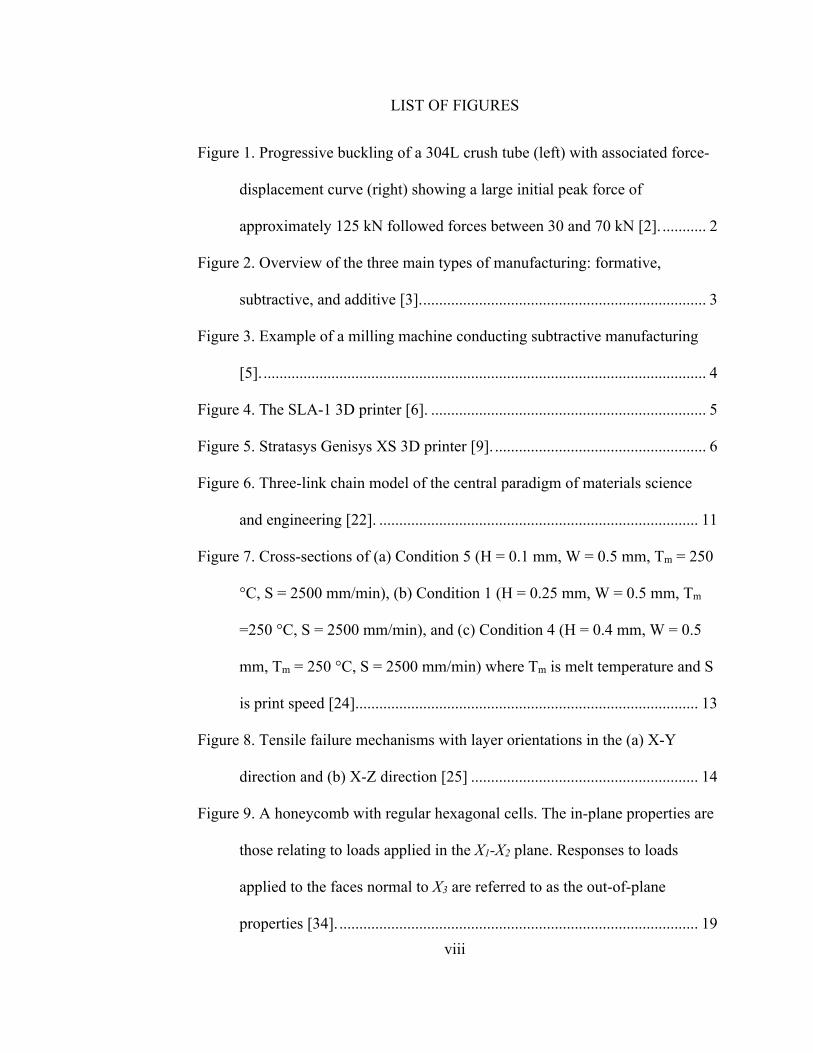
LIST OF FIGURES
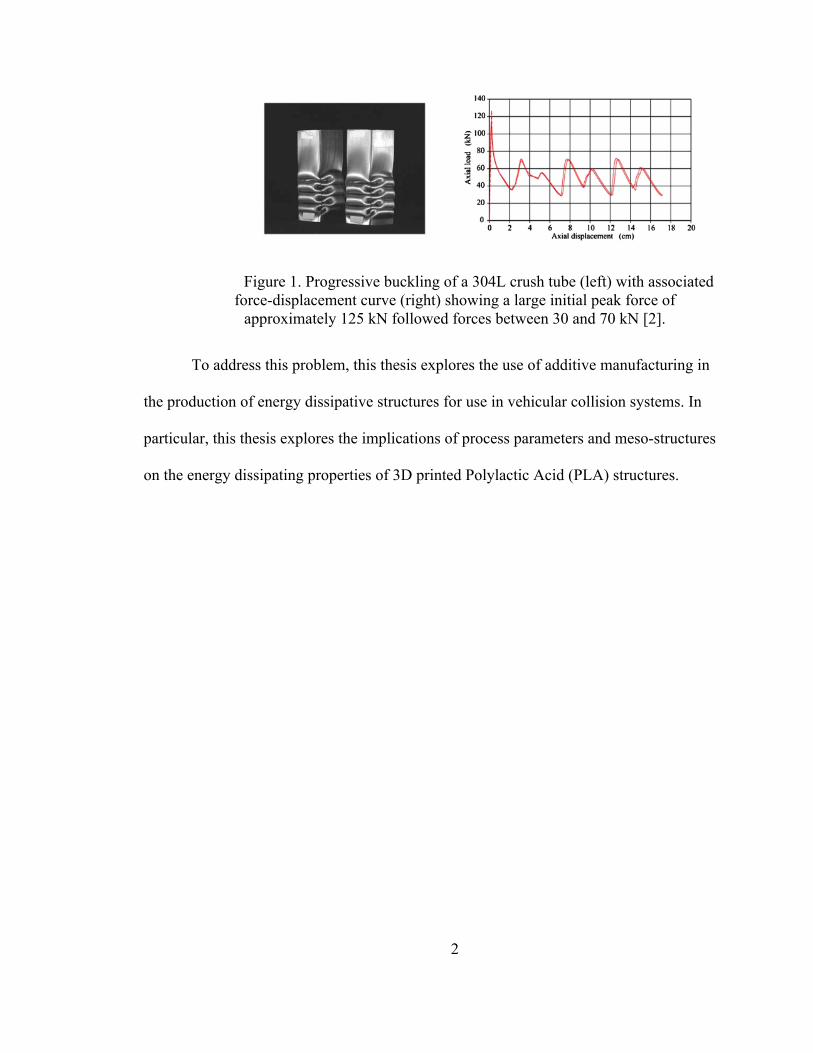
Figure 1. Progressive buckling of a 304L crush tube (left) with associated force-
displacement curve (right) showing a large initial peak force of
approximately 125 kN followed forces between 30 and 70 kN [2]. ........... 2
Figure 2. Overview of the three main types of manufacturing: formative,
subtractive, and additive [3]. ....................................................................... 3
Figure 3. Example of a milling machine conducting subtractive manufacturing
[5]. ............................................................................................................... 4
Figure 4. The SLA-1 3D printer [6]. ..................................................................... 5
Figure 5. Stratasys Genisys XS 3D printer [9]. ..................................................... 6
Figure 6. Three-link chain model of the central paradigm of materials science
and engineering [22]. ................................................................................ 11
Figure 7. Cross-sections of (a) Condition 5 (H = 0.1 mm, W = 0.5 mm, Tm = 250
°C, S = 2500 mm/min), (b) Condition 1 (H = 0.25 mm, W = 0.5 mm, Tm
=250 °C, S = 2500 mm/min), and (c) Condition 4 (H = 0.4 mm, W = 0.5
mm, Tm = 250 °C, S = 2500 mm/min) where Tm is melt temperature and S
is print speed [24]. ..................................................................................... 13
Figure 8. Tensile failure mechanisms with layer orientations in the (a) X-Y
direction and (b) X-Z direction [25] ......................................................... 14
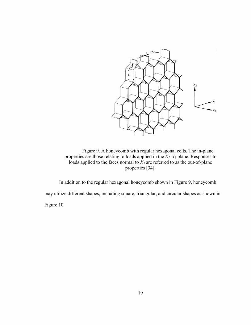
Figure 9. A honeycomb with regular hexagonal cells. The in-plane properties are
those relating to loads applied in the X1-X2 plane. Responses to loads
applied to the faces normal to X3 are referred to as the out-of-plane
properties [34]. .......................................................................................... 19
ix
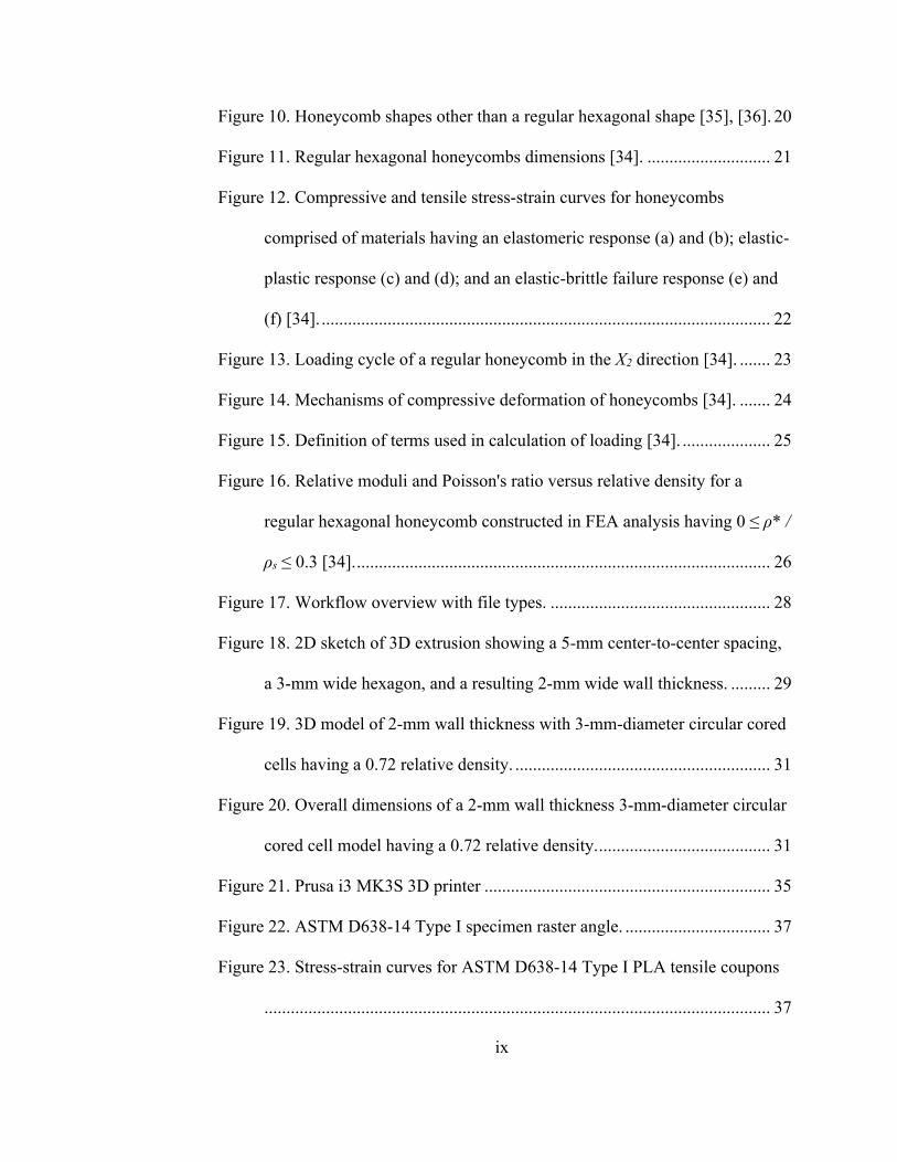
Figure 10. Honeycomb shapes other than a regular hexagonal shape [35], [36]. 20
Figure 11. Regular hexagonal honeycombs dimensions [34]. ............................ 21
Figure 12. Compressive and tensile stress-strain curves for honeycombs
comprised of materials having an elastomeric response (a) and (b); elastic-
plastic response (c) and (d); and an elastic-brittle failure response (e) and
(f) [34]. ...................................................................................................... 22
Figure 13. Loading cycle of a regular honeycomb in the X2 direction [34]. ....... 23
Figure 14. Mechanisms of compressive deformation of honeycombs [34]. ....... 24
Figure 15. Definition of terms used in calculation of loading [34]. .................... 25
Figure 16. Relative moduli and Poisson's ratio versus relative density for a
regular hexagonal honeycomb constructed in FEA analysis having 0 ≤ ρ* /
ρs ≤ 0.3 [34]. .............................................................................................. 26
Figure 17. Workflow overview with file types. .................................................. 28
Figure 18. 2D sketch of 3D extrusion showing a 5-mm center-to-center spacing,
a 3-mm wide hexagon, and a resulting 2-mm wide wall thickness. ......... 29
Figure 19. 3D model of 2-mm wall thickness with 3-mm-diameter circular cored
cells having a 0.72 relative density. .......................................................... 31
Figure 20. Overall dimensions of a 2-mm wall thickness 3-mm-diameter circular
cored cell model having a 0.72 relative density. ....................................... 31
Figure 21. Prusa i3 MK3S 3D printer ................................................................. 35
Figure 22. ASTM D638-14 Type I specimen raster angle. ................................. 37
Figure 23. Stress-strain curves for ASTM D638-14 Type I PLA tensile coupons
................................................................................................................... 37
x
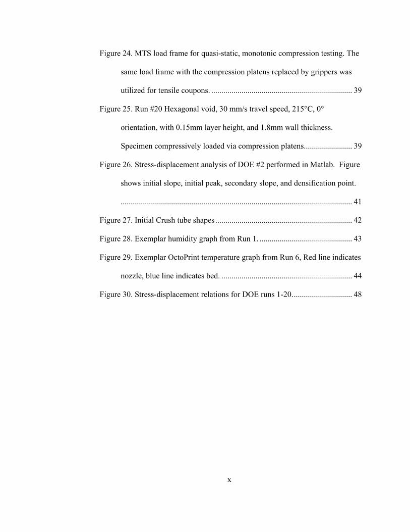
Figure 24. MTS load frame for quasi-static, monotonic compression testing. The
same load frame with the compression platens replaced by grippers was
utilized for tensile coupons. ...................................................................... 39
Figure 25. Run #20 Hexagonal void, 30 mm/s travel speed, 215°C, 0°
orientation, with 0.15mm layer height, and 1.8mm wall thickness.
Specimen compressively loaded via compression platens. ....................... 39
Figure 26. Stress-displacement analysis of DOE #2 performed in Matlab. Figure
shows initial slope, initial peak, secondary slope, and densification point.
................................................................................................................... 41
Figure 27. Initial Crush tube shapes .................................................................... 42
Figure 28. Exemplar humidity graph from Run 1. .............................................. 43
Figure 29. Exemplar OctoPrint temperature graph from Run 6, Red line indicates
nozzle, blue line indicates bed. ................................................................. 44
Figure 30. Stress-displacement relations for DOE runs 1-20. ............................. 48

xi
LIST OF TABLES
Table 1. Mechanical Properties of ABS and PLA [15]. ........................................ 9
Table 2. Properties of PLA and ABS [19]. ............................................................. 9
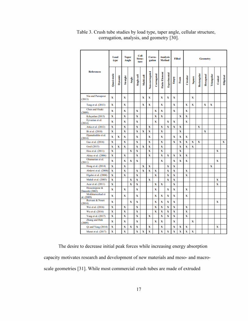
Table 3. Crush tube studies by load type, taper angle, cellular structure,
corrugation, analysis, and geometry [30]. ................................................. 17
Table 4. Ranging experiments .............................................................................. 30
Table 5. As-printed dimensions for DOE specimens. ........................................... 32
Table 6. DOE Factors ........................................................................................... 33
Table 7. Crush tube control specimens’ overall dimensions. ............................... 42
Table 8. DOE Factors ........................................................................................... 45
Table 9. Specimens showing shape of void, travel speed, nozzle temp, print
orientation, layer height and wall thickness DOE factors and levels. ...... 46
Table 10. Measured specimen height, width, wall thickness, and mass. .............. 47
Table 11. Compression test results. ..................................................................... 49
1
CHAPTER I: INTRODUCTION
With approximately 5.9 million vehicular collisions in the United States per year
[1], the ability of a vehicle to absorb energy during a collision is critical to reducing the
likelihood and severity of injuries. A primary means to absorb energy during a collision
is a crush tube, which is a predominantly prismatic shaped, metallic structure located at
either the front or rear of a vehicle intended to absorb energy via progressive buckling, as
shown in Figure 1. Progressive buckling of a 304L crush tube (left) with associated force-
displacement curve (right) showing a large initial peak force of approximately 125 kN
followed forces between 30 and 70 kN [2]. In addition to dissipating energy, crush tubes
must be lightweight to reduce vehicular green-house gas emissions, resilient to fatigue
and environmental exposure, and economically feasible to manufacture.
Historically, these competing objectives have been satisfied via extrusion,
hydroforming, or a combination of extrusion and hydroforming manufacturing processes.
Such manufacturing processes limit geometric freedom, resulting in a peak initial force
significantly greater than the mean force during progressive buckling. Thus, the problem,
i.e., crush tubes cause an excessively large initial deceleration due to the current
manufacturing process.
2
Figure 1. Progressive buckling of a 304L crush tube (left) with associated force-displacement curve (right) showing a large initial peak force of
approximately 125 kN followed forces between 30 and 70 kN [2].
To address this problem, this thesis explores the use of additive manufacturing in
the production of energy dissipative structures for use in vehicular collision systems. In
particular, this thesis explores the implications of process parameters and meso-structures
on the energy dissipating properties of 3D printed Polylactic Acid (PLA) structures.
3
Manufacturing
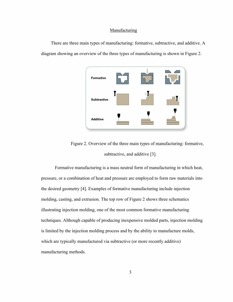
There are three main types of manufacturing: formative, subtractive, and additive. A
diagram showing an overview of the three types of manufacturing is shown in Figure 2.
Figure 2. Overview of the three main types of manufacturing: formative,
subtractive, and additive [3].
Formative manufacturing is a mass neutral form of manufacturing in which heat,
pressure, or a combination of heat and pressure are employed to form raw materials into
the desired geometry [4]. Examples of formative manufacturing include injection
molding, casting, and extrusion. The top row of Figure 2 shows three schematics
illustrating injection molding, one of the most common formative manufacturing
techniques. Although capable of producing inexpensive molded parts, injection molding
is limited by the injection molding process and by the ability to manufacture molds,
which are typically manufactured via subtractive (or more recently additive)
manufacturing methods.
4
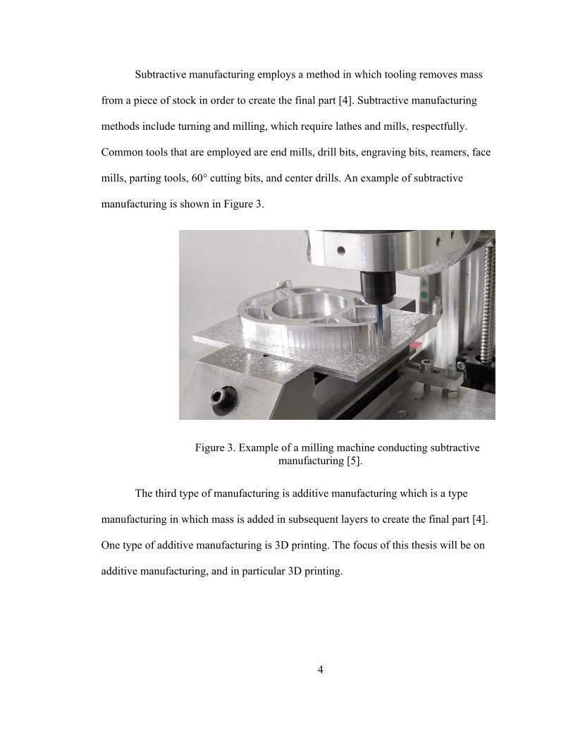
Subtractive manufacturing employs a method in which tooling removes mass
from a piece of stock in order to create the final part [4]. Subtractive manufacturing
methods include turning and milling, which require lathes and mills, respectfully.
Common tools that are employed are end mills, drill bits, engraving bits, reamers, face
mills, parting tools, 60° cutting bits, and center drills. An example of subtractive
manufacturing is shown in Figure 3.
Figure 3. Example of a milling machine conducting subtractive manufacturing [5].
The third type of manufacturing is additive manufacturing which is a type
manufacturing in which mass is added in subsequent layers to create the final part [4].
One type of additive manufacturing is 3D printing. The focus of this thesis will be on
additive manufacturing, and in particular 3D printing.

5
History of 3D Printing
Additive manufacturing, also known as 3D-printing, is one of the newest forms of
manufacturing. The idea for 3D printing was conceived in the early 1980’s by Dr.
Kodama as an alternative to rapid prototyping [6]. However, Dr. Kodama failed to enable
this patent via a viable 3D printing machine. In 1986 Charles Hull founded 3D systems
and patented Stereolithography (SLA), the first ever form of 3D printing [7]. Along with
stereolithography, Hull also created the STL file format which allows 3D printers to read
Computer Aided Design (CAD) models [7]. SLA uses UV curable resins and a UV light
to cure the resin in thin layers to form the final part. In 1988, 3D systems released the
SLA-1 shown in Figure 4.
Figure 4. The SLA-1 3D printer [6].
After the invention and subsequent success of the SLA-1 in 1991, three new
additive manufacturing (AM) technologies were commercialized. These included Fused
Deposition Modeling (FDM) by Stratasys, solid ground curing (SGC) from Cubital, and

6
laminated object manufacturing (LOM) from Helisys [8]. FDM printers use extruded
thermoplastic deposited in thin layers on top of a build plate, usually heated glass, or a
coated spring steel, to create parts. In 1996 Stratasys introduced the Genisys machine
pictured in Figure 5, which used an extrusion process similar to FDM but based on
technology developed at IBM’s Watson Research Center [8].
Figure 5. Stratasys Genisys XS 3D printer [9].
By 2002, Stratasys was the leader in FDM 3D printing and released the
Dimension line of printers, which used ABS plastic and cost $29,000 [8].
In 2008 Stratasys increased its product base for its FDM 3D printers by creating
the ABS-M30i Biocompatible 3D printer [8]. In 2009 the patent for FDM 3D printing
would expire which lead to an increase in low cost FDM printer kits as well as fully
assembled printers. The expiration of this patent meant that hobbyists could now afford
3D printers making them more mainstream and accessible [8]. In 2011, Buildatron
systems announced the availability of its RepRap-based Buildatron 1 3D printer. The
7
single material machine was offered as a kit for $1,200 and as an assembled system for
$2,000 [8]. In January 2012, MakerBot (Brooklyn, New York) released the MakerBot
Replicator, with a larger build volume than its predecessor, for $1,749. A second extruder
head option was available to print two colors or two materials within a single printed part
[8]. In 2010 the Prusa Mendel printer emerged from the RepRap community. Developed
by Josef Průša, the design of the Prusa Mendel printer iterated several times before being
sold online as a commercial kit in 2015 under as the Original Prusa i3 [10]. In 2019,
Prusa Research released the Original Prusa i3MK3S and the Original Prusa i3MK3S
(mks3) [10]. In 2021, the price of a MK3S kit was $749.00 plus shipping, and a fully
assembled and tested MK3S was $999.00 plus shipping [11]. These kits include advanced
features such as automatic bed leveling, a direct drive extruder, and upgraded bearings
and stepper motors. Thus, the printer was reliable and capable of producing high quality
prints with few surface defects. Classified as RepRap printers, Prusa printers are open-
source printers that can easily be reproduced. A common feature of RepRap machines is
3D printed components on the printer itself. This reduces cost and production times. Most
commonly RepRap machines are able to only print PLA and ABS [12]. Because of the
RepRap movement the industry has seen a reduction in fully assembled machines. While
open source printers for hobbyist cost approximately $1000, high end RepRap printers
cost up to $3000 and include features such as heated build plates and dual extruders [13].
8
Materials
The two most common materials for 3D printing are Polylactic Acid (PLA) and
Acrylonitrile butadiene styrene (ABS). While both can be used on virtually all
thermoplastic 3D printers, the materials themselves have different properties and physical
characteristics. To start with, PLA has a printing temperature of 215°C and a heat bed
temperature of 60 °C and can print in layers from 0.05 mm and up depending on nozzle
size [14]. PLA has an average ultimate strength of 56.6 MPa, and a tensile strength of
11.9 MPa [12], [15] Per ASTM D638. The material also has an average moduli of 3.37
GPa [12]. As PLA is typically made from a vegetable source such as corn [16], PLA is a
renewable thermoplastic. PLA is generally made from the melt-spinnable fibers and
therefore the advantage of both synthetic and natural fibers making it a desirable and easy
to use filament [17]. Table 1 below shows the mechanical properties of PLA and ABS. In
Table 1 it is important to note that the strengths are an average value of the test
performed in [15]. PLA has been observed to have a tensile strength range of 8.00-103
MPa [18]. Table 2 shows the common printing properties of each material.

9
Table 1. Mechanical Properties of ABS and PLA [15].
Table 2. Properties of PLA and ABS [19].
Because it is made of natural ingredients, PLA has fewer health risks than ABS
when printed in poorly ventilated areas [13]. PLA is also stronger than ABS but is more
brittle and has a lower coefficient of thermal expansion making ideally suited for energy
absorption [13]. Although stronger and stiffer than ABS, PLA’s 50 to 140 ℃ deflection
temperature as determined by ASTM D 648 is less than ABS’s 68°C to 100°C deflection
temperature [13].
10
One great advantage of PLA is its cost. In 2014, the cost for a 1 kg spool of PLA
was approximately $50; today a 1 kg spool is $24.99 [20], [21]. This is a 50% reduction
in cost in only seven years which makes PLA an affordable option for manufacturing.
Process-Structure-Property-Performance Mappings
General PSPP Approach
Materials science, engineering, manufacturing, and design are often viewed from
a processing, structure, properties, and performance (PSPP) paradigm based upon Olsen
[22]. PSPP forms a set of cause-and-effect relationships between length scales and
manufacturing processes required to satisfy an overarching performance requirement
[22]. When compared to length scales, there is a spectrum of characteristic relaxation
times so that in every real structure there is a small level that has not had time to
equilibrate [22]. As shown in Figure 6, PSPP mappings define deductive relationships
that seek to accurately define cause-and-effect relations in a bottom up and manner while
simultaneously providing a searchable inductive path to determine processes, structures,
and properties that satisfy the top-down inductive design objectives.

11
Figure 6. Three-link chain model of the central paradigm of materials science and engineering [22].
When talking about materials the common practice of empirical development
involves little up front analysis and large amounts of simultaneous evaluation of
prototypes [22]. This eventually leads to the empirical correlation that produced materials
with little predictability in behavior. In today’s market, experimentation and prototyping
lead to increased costs while computational based theory and design have seen a decrease
in cost. This is where PSPP has proven valuable as companies look to develop new
materials for less money.
Voigt-Reuss Equations for Estimating Stiffness
Upper and lower bounds of the stiffness of a composite may be estimated via
Voigt-Reuss equations [23]. The upper bound can be estimated by assuming the
microstructure is aligned parallel to the loading direction, i.e.,
12
𝐸!,∥ = 𝐸$%&𝑓$%& + 𝐸'()𝑓'() (1)
where 𝐸!,∥ is the upper bound of the stiffness of the composite, 𝐸$%& is the
stiffness of the neat PLA, 𝑓$%& is the volume fraction of the PLA, 𝐸'() is the stiffness of
the air, and 𝑓'() is the volume fraction of air. The lower bound of stiffness can be
estimated by assuming the microstructure is oriented perpendicular to the loading
direction, i.e.,
1𝐸*,⫠
=𝑓$%&𝐸$%&
+𝑓'()𝐸'()
(2)
where 𝐸*,⫠is the stiffness of the composite with the microstructure aligned
perpendicular to the loading direction. Calculation of the lower bound of composite
stiffness is hindered by the lack of air having a measurable stiffness.
Effects of Layer Thickness
Layer thickness can have a great impact on the strength of components. Low
interlayer strength is caused by insufficient interlayer contact and a lack of interlayer
polymer diffusion [24]. The interlayer contact between materials was originally modeled
as a wetting process. This means that the materials are bonded due to surface tension.
This model however has recently been disproved as it has been discovered that the
surface tension forces are hindered by the rapid cooling of layers and roads [24]. One of
the new models is one in which the model is held together by in-line pressure and
temperature between layers as well as diffusion. Coogan and Kazmer’s [24] results,

13
shown here as Figure 7, showed that bond width and therefore bond strength were
functions of contact pressure between the extrudate and the previous layer.
Figure 7. Cross-sections of (a) Condition 5 (H = 0.1 mm, W = 0.5 mm, Tm = 250 °C, S = 2500 mm/min), (b) Condition 1 (H = 0.25 mm, W = 0.5 mm, Tm
=250 °C, S = 2500 mm/min), and (c) Condition 4 (H = 0.4 mm, W = 0.5 mm, Tm = 250 °C, S = 2500 mm/min) where Tm is melt temperature and S is print speed
[24].
As can be seen in Figure 7, the smaller the layer height the tighter the layer bond.
Coogan and Kazmer [24] theorized that when a new layer is added to the printed
substrate, the previous interface is re-heated slightly allowing for greater bond between
layers. This theory is supported by results presented in Torres et al. [25]. When similar
specimens were tested the layer thickness had the second greatest effect on the strength.
It was noted that as the layer thickness was decreased strength increased. This was
reported as an effect of the bond between layers. An example of Torres et Al.’s [25]
tensile failure results of the experiment are shown in Figure 8.
14
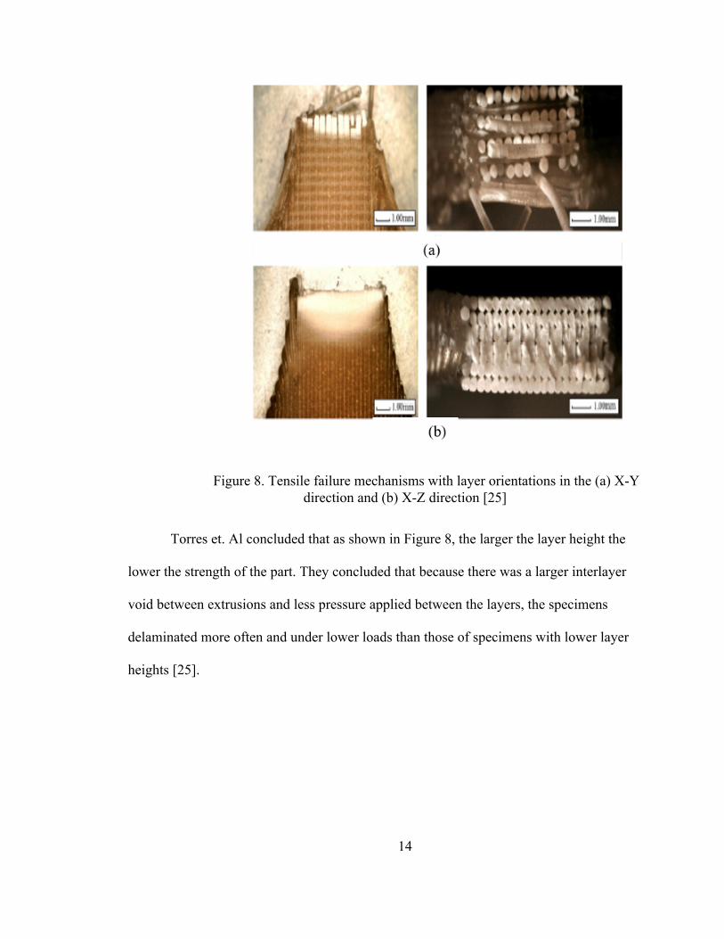
Figure 8. Tensile failure mechanisms with layer orientations in the (a) X-Y direction and (b) X-Z direction [25]
Torres et. Al concluded that as shown in Figure 8, the larger the layer height the
lower the strength of the part. They concluded that because there was a larger interlayer
void between extrusions and less pressure applied between the layers, the specimens
delaminated more often and under lower loads than those of specimens with lower layer
heights [25].
15
Energy Dissipative Structures
One type of mechanical energy dissipative structures are crush tubes. Crush tubes
are generally extruded structures that absorb energy upon impact. Crush tubes are ideally
an energy-absorbing structure that would dissipate the kinetic energy of an impact, while
transmitting a constant plateau force, within safe ranges of deceleration, to the supporting
structure [26]. What this means is that during impact the structure actually compresses to
absorb the impact and slow the deceleration gradually thus imparting less force on the
attached structure to be protected. Crush tubes are used in a wide variety of industries.
For example, car manufactures use them to increase crash safety, and in the aerospace
field crush tubes are highly sought after as structural components because they provide a
combination of lightweight characteristics, high stiffness, energy absorption, and fracture
toughness for extreme loading conditions [27]. Coincidentally, recent advances in the
defense, aerospace, automotive, semiconductor, and energy industries have triggered a
tremendous demand for high-performance materials with lightweight and enhanced
mechanical properties [27].
Automotive Industry
There are approximately 5.9 million vehicular collisions in the United States per
year [1], of which air bags fail to deploy in approximately 18% of all collisions [28]. In
total, the 5.9 million collisions result in approximately 36,560 deaths per year [29]. This
leads car developers to seek additional means of decelerating vehicles during impact to
reduce the chance of injuries. One way that they have been able to do this is by utilizing

16
crush tubes. The ideal shape and material for crush tubes is a topic of interest, and has
been studied by multiple researchers, as shown in Table 3.
17
Table 3. Crush tube studies by load type, taper angle, cellular structure, corrugation, analysis, and geometry [30].
The desire to decrease initial peak forces while increasing energy absorption
capacity motivates research and development of new materials and meso- and macro-
scale geometries [31]. While most commercial crush tubes are made of extruded
18
aluminum or stainless steel, there are variations. One such variation is produced using
high strength carbon fiber [32]. Carbon fiber has an ultimate tensile strength of 3790 MPa
and an elastic modulus of 230 GPa when tested at 0.176 mm thick [32]. This new method
for manufacturing crush tubes allows for greater energy impact with lower weight added
to vehicles. This is useful for engineers as they attempt to lightweight vehicles in order to
increase fuel efficiency. Other than changing the material engineers have been working
on using different shapes and cuts to increase the energy absorption of the crush tubes.
For example, Subramaniyan et al. [33] determined that enhanced geometry (e.g., groves,
corrugated tubes, special patterns, or cutting holes) could achieve greater buckling and
energy absorption with a lower peak force. The addition of these of these initiation
methods has led to the need for a new type of manufacturing for production.
Cellular Solids
One way of increasing energy absorption is by using cellular solids. Compared
with bulk materials, cellular structures and lattice solids can be designed to possess all
these desired properties [27]. One type of cellular solid is a honeycomb which can be
seen in Figure 9. A honeycomb is characterized as any 1D extrusion of a 2D shape with
the 2D shape having a plurality of equally spaced voids having any possible topology
[34]. Honeycombs have been used in a variety of applications, including energy-
absorbing crushable feet for the Apollo 11 landing module to catalyst carriers for heat
exchanges [34].
19
Figure 9. A honeycomb with regular hexagonal cells. The in-plane properties are those relating to loads applied in the X1-X2 plane. Responses to
loads applied to the faces normal to X3 are referred to as the out-of-plane properties [34].
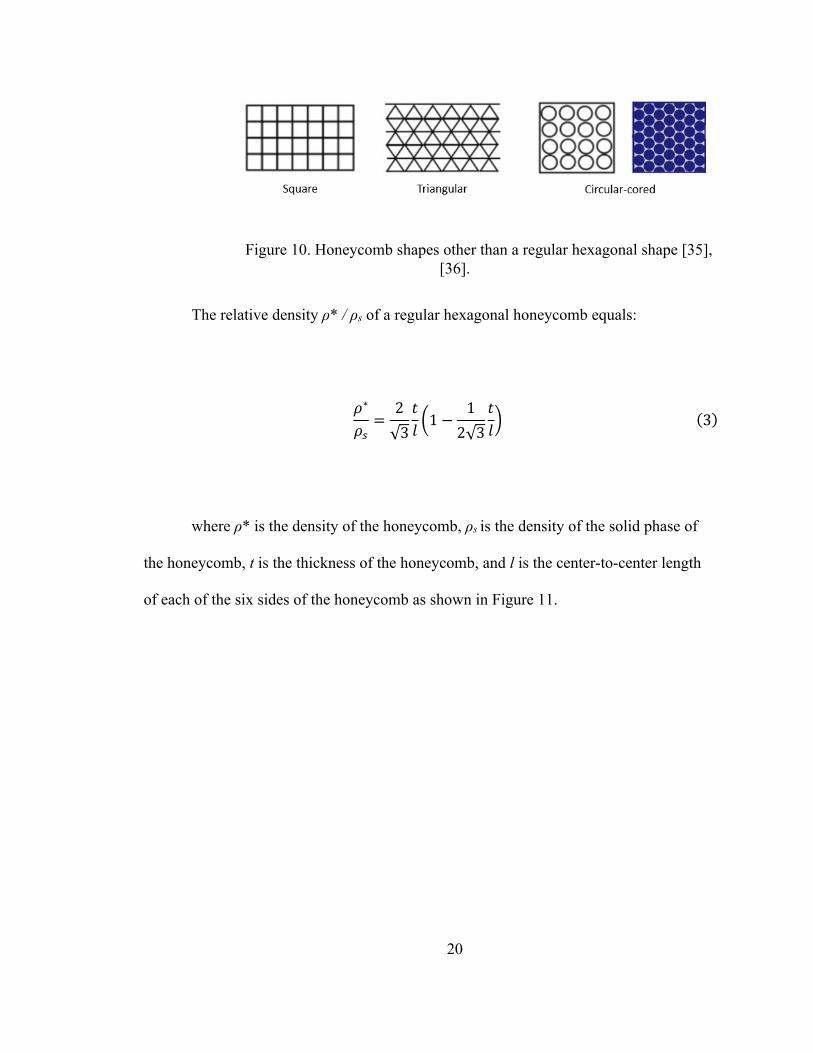
In addition to the regular hexagonal honeycomb shown in Figure 9, honeycomb
may utilize different shapes, including square, triangular, and circular shapes as shown in
Figure 10.
20
Figure 10. Honeycomb shapes other than a regular hexagonal shape [35], [36].
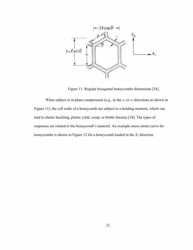
The relative density ρ* / ρs of a regular hexagonal honeycomb equals:
𝜌∗
𝜌-=
2√3
𝑡𝑙 /1 −
12√3
𝑡𝑙1
(3)
where ρ* is the density of the honeycomb, ρs is the density of the solid phase of
the honeycomb, t is the thickness of the honeycomb, and l is the center-to-center length
of each of the six sides of the honeycomb as shown in Figure 11.
21
Figure 11. Regular hexagonal honeycombs dimensions [34].
When subject to in plane compression (e.g., in the x1 or x2 directions as shown in
Figure 11), the cell walls of a honeycomb are subject to a bending moment, which can
lead to elastic buckling, plastic yield, creep, or brittle fracture [34]. The types of
responses are related to the honeycomb’s material. An example stress-strain curve for
honeycombs is shown in Figure 12 for a honeycomb loaded in the X2 direction.
22
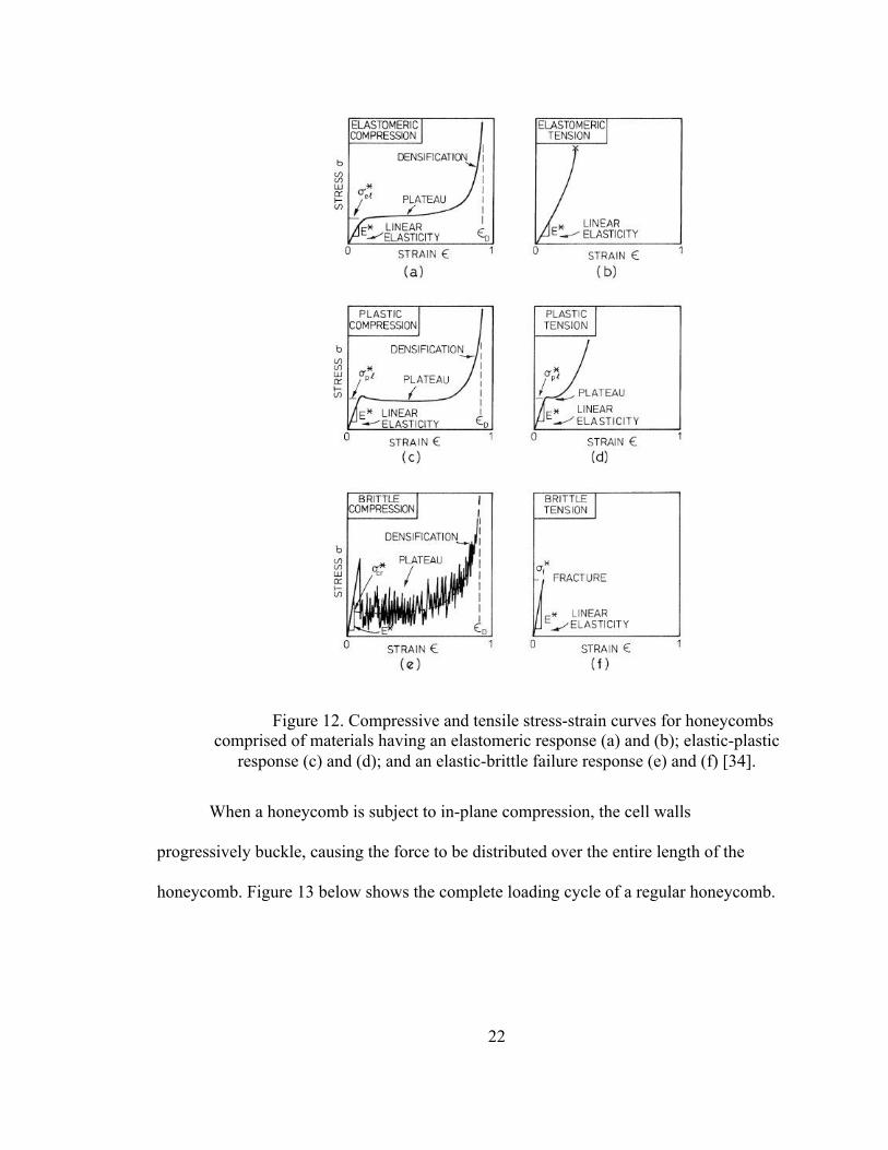
Figure 12. Compressive and tensile stress-strain curves for honeycombs comprised of materials having an elastomeric response (a) and (b); elastic-plastic
response (c) and (d); and an elastic-brittle failure response (e) and (f) [34].
When a honeycomb is subject to in-plane compression, the cell walls
progressively buckle, causing the force to be distributed over the entire length of the
honeycomb. Figure 13 below shows the complete loading cycle of a regular honeycomb.
23
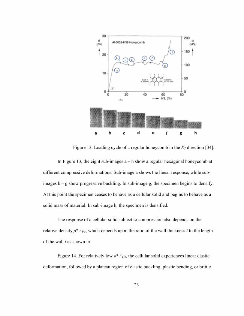
Figure 13. Loading cycle of a regular honeycomb in the X2 direction [34].
In Figure 13, the eight sub-images a – h show a regular hexagonal honeycomb at
different compressive deformations. Sub-image a shows the linear response, while sub-
images b – g show progressive buckling. In sub-image g, the specimen begins to densify.
At this point the specimen ceases to behave as a cellular solid and begins to behave as a
solid mass of material. In sub-image h, the specimen is densified.
The response of a cellular solid subject to compression also depends on the
relative density ρ* / ρs, which depends upon the ratio of the wall thickness t to the length
of the wall l as shown in
Figure 14. For relatively low ρ* / ρs, the cellular solid experiences linear elastic
deformation, followed by a plateau region of elastic buckling, plastic bending, or brittle
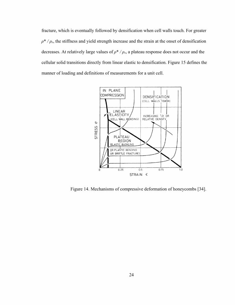
24
fracture, which is eventually followed by densification when cell walls touch. For greater
ρ* / ρs, the stiffness and yield strength increase and the strain at the onset of densification
decreases. At relatively large values of ρ* / ρs, a plateau response does not occur and the
cellular solid transitions directly from linear elastic to densification. Figure 15 defines the
manner of loading and definitions of measurements for a unit cell.
Figure 14. Mechanisms of compressive deformation of honeycombs [34].
25
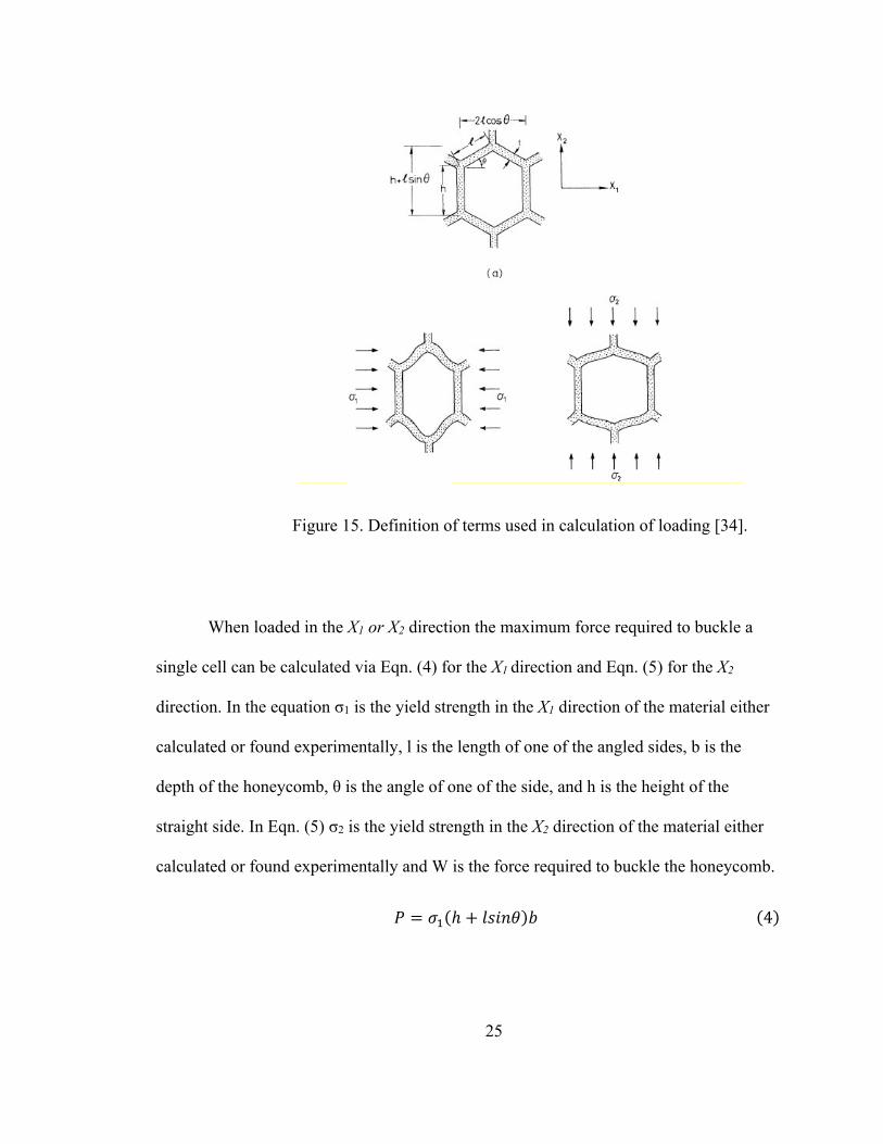
Figure 15. Definition of terms used in calculation of loading [34].
When loaded in the X1 or X2 direction the maximum force required to buckle a
single cell can be calculated via Eqn. (4) for the X1 direction and Eqn. (5) for the X2
direction. In the equation σ1 is the yield strength in the X1 direction of the material either
calculated or found experimentally, l is the length of one of the angled sides, b is the
depth of the honeycomb, θ is the angle of one of the side, and h is the height of the
straight side. In Eqn. (5) σ2 is the yield strength in the X2 direction of the material either
calculated or found experimentally and W is the force required to buckle the honeycomb.
𝑃 = 𝜎.(ℎ + 𝑙𝑠𝑖𝑛𝜃)𝑏 (4)
26
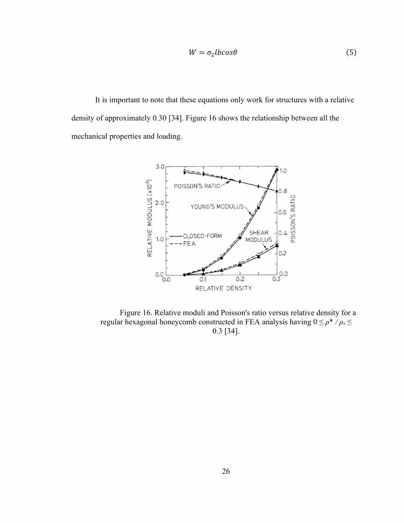
𝑊 = 𝜎/𝑙𝑏𝑐𝑜𝑠𝜃 (5)
It is important to note that these equations only work for structures with a relative
density of approximately 0.30 [34]. Figure 16 shows the relationship between all the
mechanical properties and loading.
Figure 16. Relative moduli and Poisson's ratio versus relative density for a regular hexagonal honeycomb constructed in FEA analysis having 0 ≤ ρ* / ρs ≤
0.3 [34].

27
CHAPTER II: MEANS AND METHODS
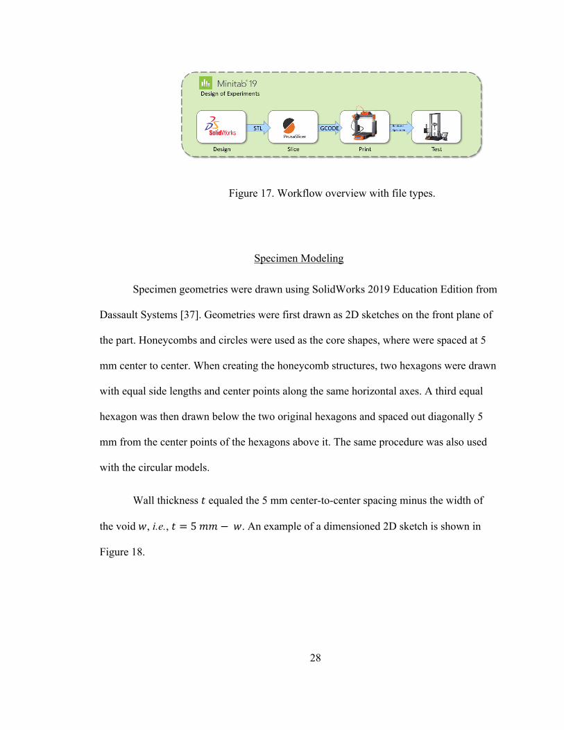
The influence of process and meso-structure on honeycomb properties were
determined via a Design of Experiments (DOE) approach implemented via the workflow
shown in Figure 17. Starting at the left side within Figure 17, six parametric models were
drawn and converted to STL files within Solidworks before being sliced via PrusaSlicer.
Here, “sliced” is defined as a method of converting the process-agnostic STL geometric
file to a GCODE file containing 3D-printer machine instructions in which process
parameters (e.g., print orientation, extruder temperature, and print head speed) have been
defined by the user. Imbuing process parameters into the sliced GCODE files resulted in
a total of 20 sliced GCODE files. The sliced GCODE files were then transferred to an SD
card, which was then input into the 3D printer. The 3D printer then executed (i.e.,
“printed”) the GCODE commands to create a realized specimen. Realized specimens
were tested on an MTS Criterion C43.504 load frame with a 50 KN load cell moving at
0.003 in/s, which output raw force-displacement data in CSV format. The CSV files were
then read by a Matlab script which analyzed the data and wrote the results to an MS
Excel file. Data were then imputed into Minitab to estimate the response surfaces via
multi-linear regression analysis.
28
Figure 17. Workflow overview with file types.
Specimen Modeling
Specimen geometries were drawn using SolidWorks 2019 Education Edition from
Dassault Systems [37]. Geometries were first drawn as 2D sketches on the front plane of
the part. Honeycombs and circles were used as the core shapes, where were spaced at 5
mm center to center. When creating the honeycomb structures, two hexagons were drawn
with equal side lengths and center points along the same horizontal axes. A third equal
hexagon was then drawn below the two original hexagons and spaced out diagonally 5
mm from the center points of the hexagons above it. The same procedure was also used
with the circular models.
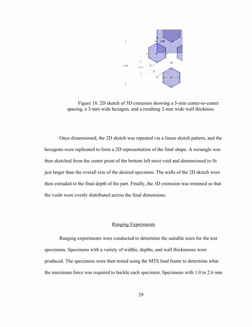
Wall thickness 𝑡 equaled the 5 mm center-to-center spacing minus the width of
the void 𝑤, i.e., 𝑡 = 5𝑚𝑚 − 𝑤. An example of a dimensioned 2D sketch is shown in
Figure 18.
29
Figure 18. 2D sketch of 3D extrusion showing a 5-mm center-to-center spacing, a 3-mm wide hexagon, and a resulting 2-mm wide wall thickness.
Once dimensioned, the 2D sketch was repeated via a linear sketch pattern, and the
hexagons were replicated to form a 2D representation of the final shape. A rectangle was
then sketched from the center point of the bottom left most void and dimensioned to fit
just larger than the overall size of the desired specimen. The walls of the 2D sketch were
then extruded to the final depth of the part. Finally, the 3D extrusion was trimmed so that
the voids were evenly distributed across the final dimensions.
Ranging Experiments
Ranging experiments were conducted to determine the suitable sizes for the test
specimens. Specimens with a variety of widths, depths, and wall thicknesses were
produced. The specimens were then tested using the MTS load frame to determine what
the maximum force was required to buckle each specimen. Specimens with 1.0 to 2.6 mm
30
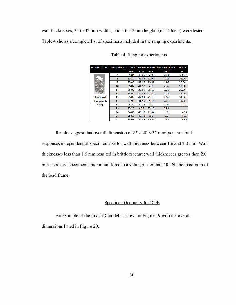
wall thicknesses, 21 to 42 mm widths, and 5 to 42 mm heights (cf. Table 4) were tested.
Table 4 shows a complete list of specimens included in the ranging experiments.
Table 4. Ranging experiments
Results suggest that overall dimension of 85 × 40 × 35 mm3 generate bulk
responses independent of specimen size for wall thickness between 1.6 and 2.0 mm. Wall
thicknesses less than 1.6 mm resulted in brittle fracture; wall thicknesses greater than 2.0
mm increased specimen’s maximum force to a value greater than 50 kN, the maximum of
the load frame.
Specimen Geometry for DOE
An example of the final 3D model is shown in Figure 19 with the overall
dimensions listed in Figure 20.

31
Figure 19. 3D model of 2-mm wall thickness with 3-mm-diameter circular cored cells having a 0.72 relative density.
Figure 20. Overall dimensions of a 2-mm wall thickness 3-mm-diameter circular cored cell model having a 0.72 relative density.
All models were nominally 40-mm wide, 35-mm deep, and 85-mm tall. The width
was chosen to be wide enough so that there was at least half of the wall thickness at the
X
X
Y
X
32
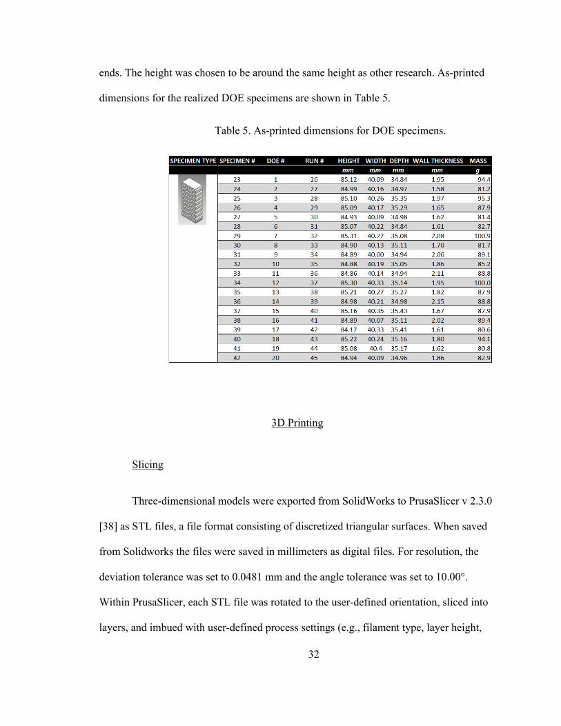
ends. The height was chosen to be around the same height as other research. As-printed
dimensions for the realized DOE specimens are shown in Table 5.
Table 5. As-printed dimensions for DOE specimens.
3D Printing
Slicing
Three-dimensional models were exported from SolidWorks to PrusaSlicer v 2.3.0
[38] as STL files, a file format consisting of discretized triangular surfaces. When saved
from Solidworks the files were saved in millimeters as digital files. For resolution, the
deviation tolerance was set to 0.0481 mm and the angle tolerance was set to 10.00°.
Within PrusaSlicer, each STL file was rotated to the user-defined orientation, sliced into
layers, and imbued with user-defined process settings (e.g., filament type, layer height,
33
bed temperature, nozzle temperature, print head speed, flow rate, infill, and wall
thickness) before being exported as a GCODE file for the Prusa i3 MK3S 3D printer.
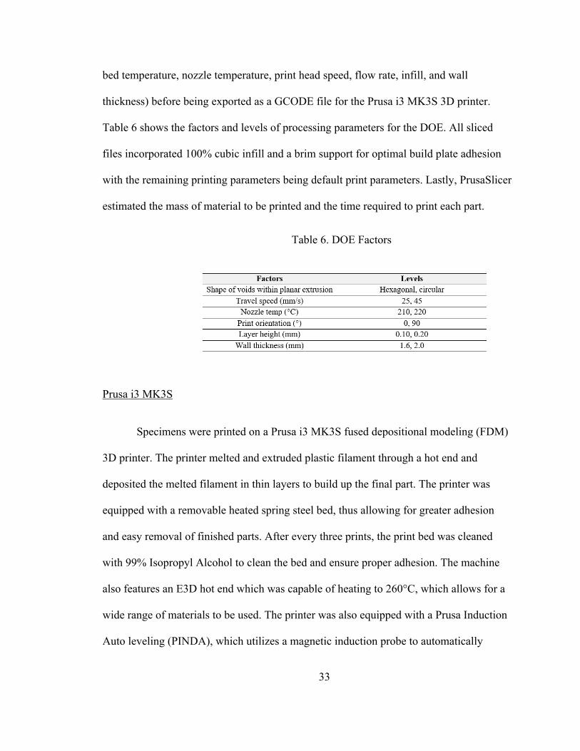
Table 6 shows the factors and levels of processing parameters for the DOE. All sliced
files incorporated 100% cubic infill and a brim support for optimal build plate adhesion
with the remaining printing parameters being default print parameters. Lastly, PrusaSlicer
estimated the mass of material to be printed and the time required to print each part.
Table 6. DOE Factors
Prusa i3 MK3S
Specimens were printed on a Prusa i3 MK3S fused depositional modeling (FDM)
3D printer. The printer melted and extruded plastic filament through a hot end and
deposited the melted filament in thin layers to build up the final part. The printer was
equipped with a removable heated spring steel bed, thus allowing for greater adhesion
and easy removal of finished parts. After every three prints, the print bed was cleaned
with 99% Isopropyl Alcohol to clean the bed and ensure proper adhesion. The machine
also features an E3D hot end which was capable of heating to 260°C, which allows for a
wide range of materials to be used. The printer was also equipped with a Prusa Induction
Auto leveling (PINDA), which utilizes a magnetic induction probe to automatically
34
measure and level the bed before every print, thus ensuring the print bed to be within 0.07
mm of level and reducing the chance of delamination. The machine also included a direct
drive filament feeder for retraction control and fewer stings during printing. The i3
MK3S also included a filament runout sensor, auto homing extruder, and crash detection.
The printer was equipped with a 0.4-mm-diameter brass nozzle for detailed printing. The
machine also featured a filament cooling fan which allows for optimal layer adhesion.
The machine was capable of holding tolerances of ± 0.03 mm. The printer has a build
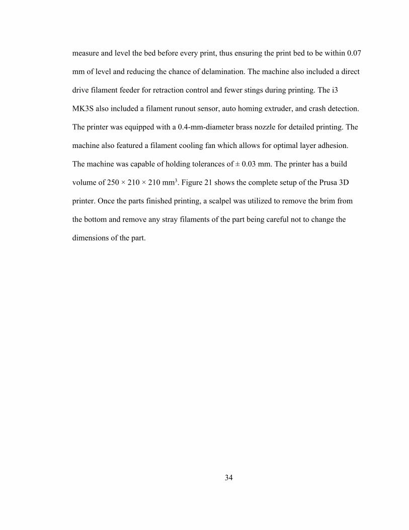
volume of 250 × 210 × 210 mm3. Figure 21 shows the complete setup of the Prusa 3D
printer. Once the parts finished printing, a scalpel was utilized to remove the brim from
the bottom and remove any stray filaments of the part being careful not to change the
dimensions of the part.
35
Figure 21. Prusa i3 MK3S 3D printer
PLA Material
Specimens were printed using Prusament 1.75-mm-diameter polylactic acid
(PLA) filament. Prusament filament was chosen due to its reported tighter diametrical
tolerances [39]. The filament was supplied in 1-kg rolls and included factory batch testing
data for tensile strength and overall dimensions of the filament. The rolls were kept
sealed in original packaging until needed and once opened were stored in a humidity
controlled dry box to prevent the filament from drying out. Prusament filament has a
nominal 2.3-GPa modulus and a 37.6-MPa yield strength [39]. Although Prusa doesn’t
state the ultimate strength of Prusament PLA, a typical ultimate tensile strength of PLA is
46 MPa [18].
Roll of filament
Extruder with PINDA probe
Heated spring steel PEI bed
LCD screen
Einsy RAMBo
36
Tensile Tests
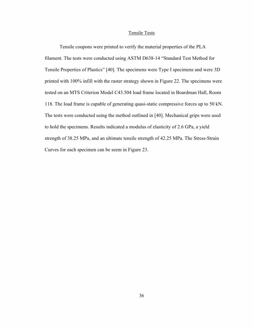
Tensile coupons were printed to verify the material properties of the PLA
filament. The tests were conducted using ASTM D638-14 “Standard Test Method for
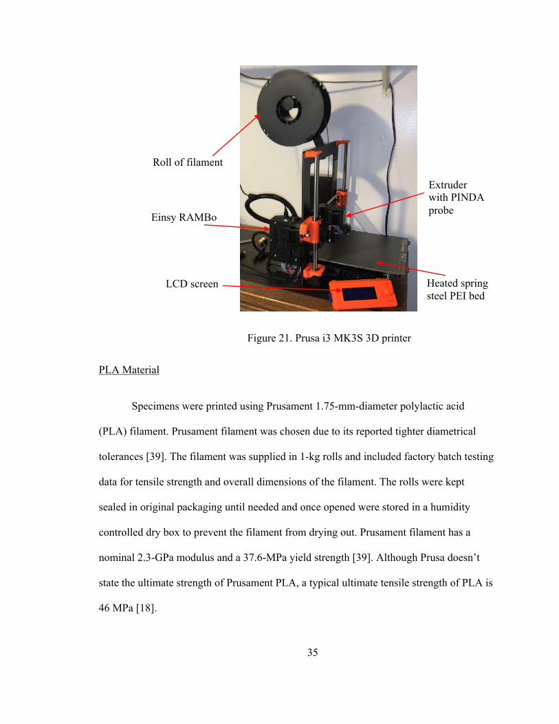
Tensile Properties of Plastics” [40]. The specimens were Type I specimens and were 3D
printed with 100% infill with the raster strategy shown in Figure 22. The specimens were
tested on an MTS Criterion Model C43.504 load frame located in Boardman Hall, Room
118. The load frame is capable of generating quasi-static compressive forces up to 50 kN.
The tests were conducted using the method outlined in [40]. Mechanical grips were used
to hold the specimens. Results indicated a modulus of elasticity of 2.6 GPa, a yield
strength of 38.25 MPa, and an ultimate tensile strength of 42.25 MPa. The Stress-Strain
Curves for each specimen can be seem in Figure 23.
37
Figure 22. ASTM D638-14 Type I specimen raster angle.
Figure 23. Stress-strain curves for ASTM D638-14 Type I PLA tensile
coupons
38
Load Frame Testing of Honeycomb Specimens
Honeycomb specimens were tested using an MTS Criterion Model C43.504 load
frame located in Boardman Hall, Room 118. The load frame is capable of generating
quasi-static compressive forces up to 50 kN; has a minimum and maximum crosshead
travel speeds of 0.005 mm/min and 750 mm/min, respectively; has the required
compression platens; and records force and crosshead deflection data [41]. A custom
compression test was created and stored in the MTS TWE test suit on the load frame’s
computer. The specimens were loaded between the compression platens and a uniform
force was applied to the top and bottom of the specimens. The crosshead rate and data
acquisition rates were 0.003 in/s and 10 Hz, respectively. Each specimen was preloaded
to 5 lbf before each test. The force and displacement from the tests were recorded in the
TWE suit and a force displacement graph was created as the tests were conducted. Each
specimen was loaded for 500 seconds, until densification, or until failure. Videos of each
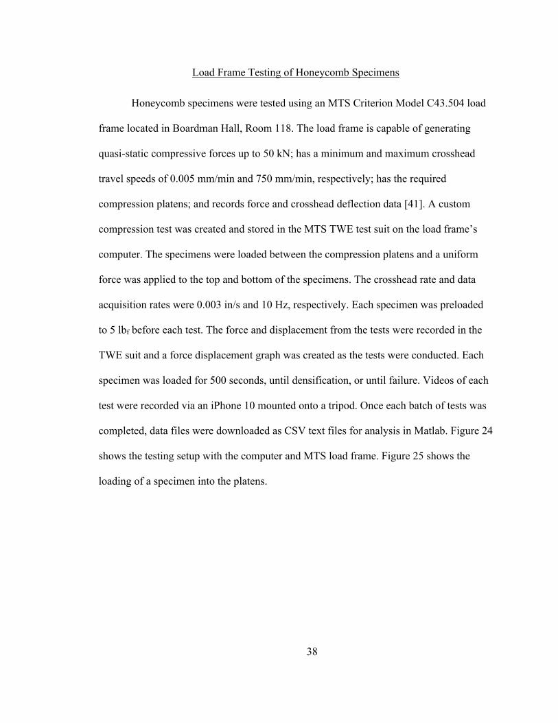
test were recorded via an iPhone 10 mounted onto a tripod. Once each batch of tests was
completed, data files were downloaded as CSV text files for analysis in Matlab. Figure 24
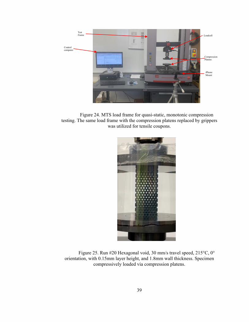
shows the testing setup with the computer and MTS load frame. Figure 25 shows the
loading of a specimen into the platens.
39
Figure 24. MTS load frame for quasi-static, monotonic compression testing. The same load frame with the compression platens replaced by grippers
was utilized for tensile coupons.
Figure 25. Run #20 Hexagonal void, 30 mm/s travel speed, 215°C, 0° orientation, with 0.15mm layer height, and 1.8mm wall thickness. Specimen
compressively loaded via compression platens.
Loadcell
Compression Platens
iPhone Mount
Test Frame
Control computer

40
Analysis Methods
A custom MATLAB script was written to analyze the raw .TXT data files. The
script reads measured specimen dimensions from an Excel data file to convert measured
force data to stress data. The MATLAB script also calculates the start point and end
points for linear elastic region by numerically calculating a backwards 2nd derivative of
stress as a function of displacement. The 1st and 2nd derivatives utilize 5-consecutive data
point running average to smooth out numerical noise in the raw data. The start point for
the initial slope is then calculated as the first point in which the backwards 2nd derivative
is within 5% of zero; the stop point for the initial slope is the last point in which the
backwards 2nd derivative is within 5% of zero.
The slope within the plastic region is calculated by first calculating the initial
peak force and then identifying the first local minimum stress occurring after the initial
peak force. The stress for the start of the slope within the plastic region equals the local
minimum stress immediately after the initial peak stress plus a quarter of the sum of the
initial peak stress minus the local minimum stress. The stop point for the second slope is
defined manually via inspection and is stored in the Excel sheet for each data file. All of
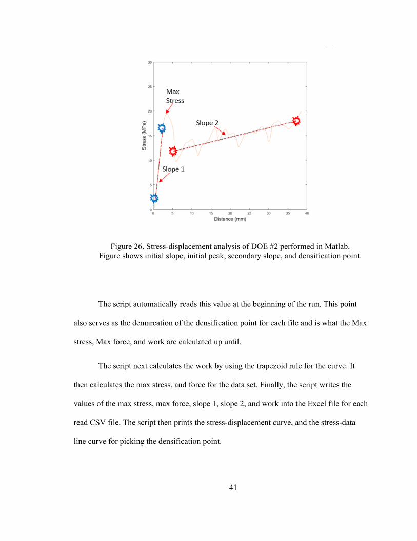
this can be seen in Figure 26.
41
Figure 26. Stress-displacement analysis of DOE #2 performed in Matlab. Figure shows initial slope, initial peak, secondary slope, and densification point.
The script automatically reads this value at the beginning of the run. This point
also serves as the demarcation of the densification point for each file and is what the Max
stress, Max force, and work are calculated up until.
The script next calculates the work by using the trapezoid rule for the curve. It
then calculates the max stress, and force for the data set. Finally, the script writes the
values of the max stress, max force, slope 1, slope 2, and work into the Excel file for each
read CSV file. The script then prints the stress-displacement curve, and the stress-data
line curve for picking the densification point.
42
Once inside of Minitab, the results were analyzed against the Design of
Experiments matrix. The data for each was compared at a 95% confidence interval
assuming initial three-way interaction regression models. Reduced order regression
models were generated by successively removing the least-significant main effect, two-
way interaction, or three-way interaction term until only the statistically-significant terms
remained.
Initial Experiments
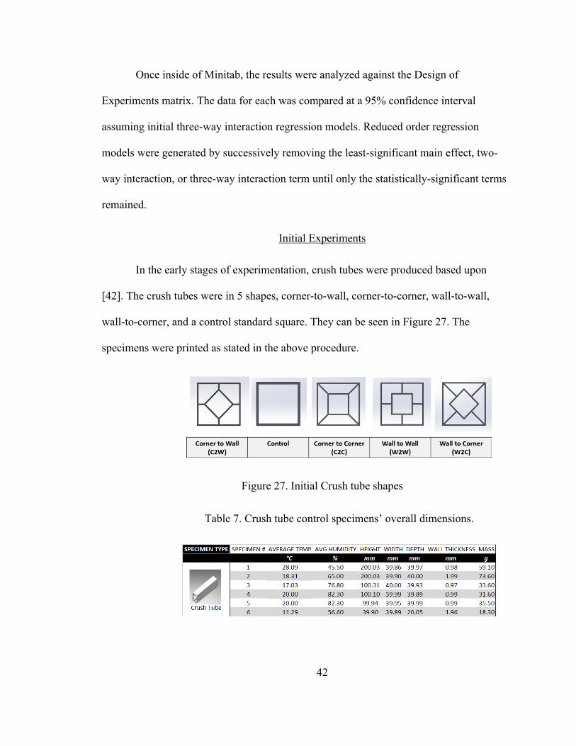
In the early stages of experimentation, crush tubes were produced based upon
[42]. The crush tubes were in 5 shapes, corner-to-wall, corner-to-corner, wall-to-wall,
wall-to-corner, and a control standard square. They can be seen in Figure 27. The
specimens were printed as stated in the above procedure.
Figure 27. Initial Crush tube shapes
Table 7. Crush tube control specimens’ overall dimensions.
43
Measurement Techniques
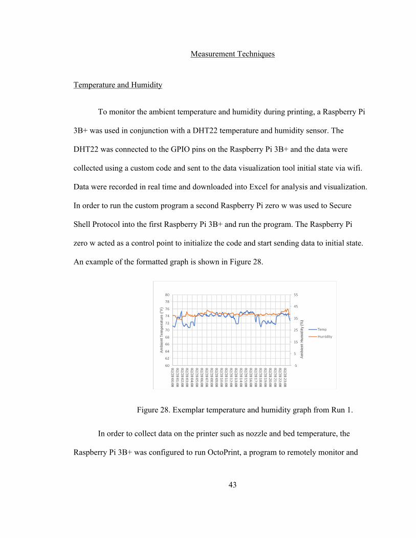
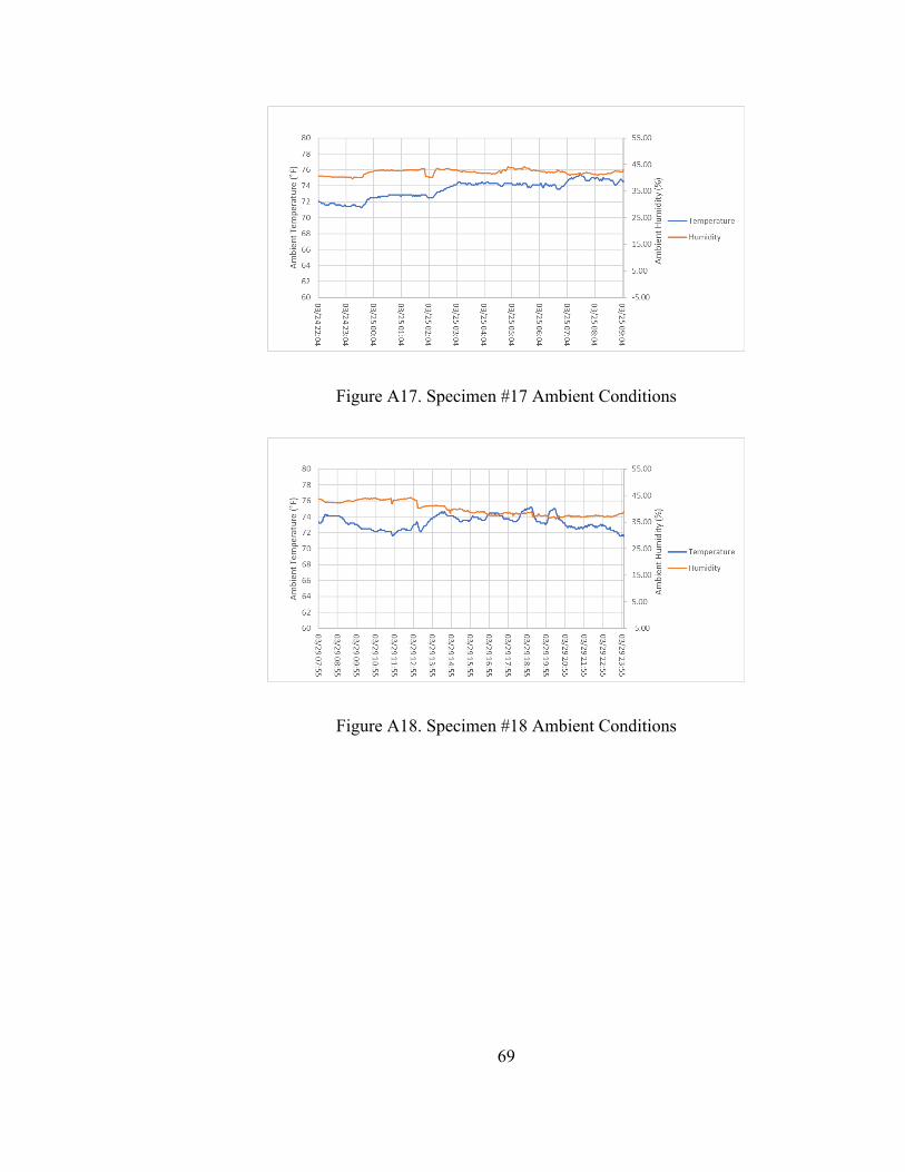
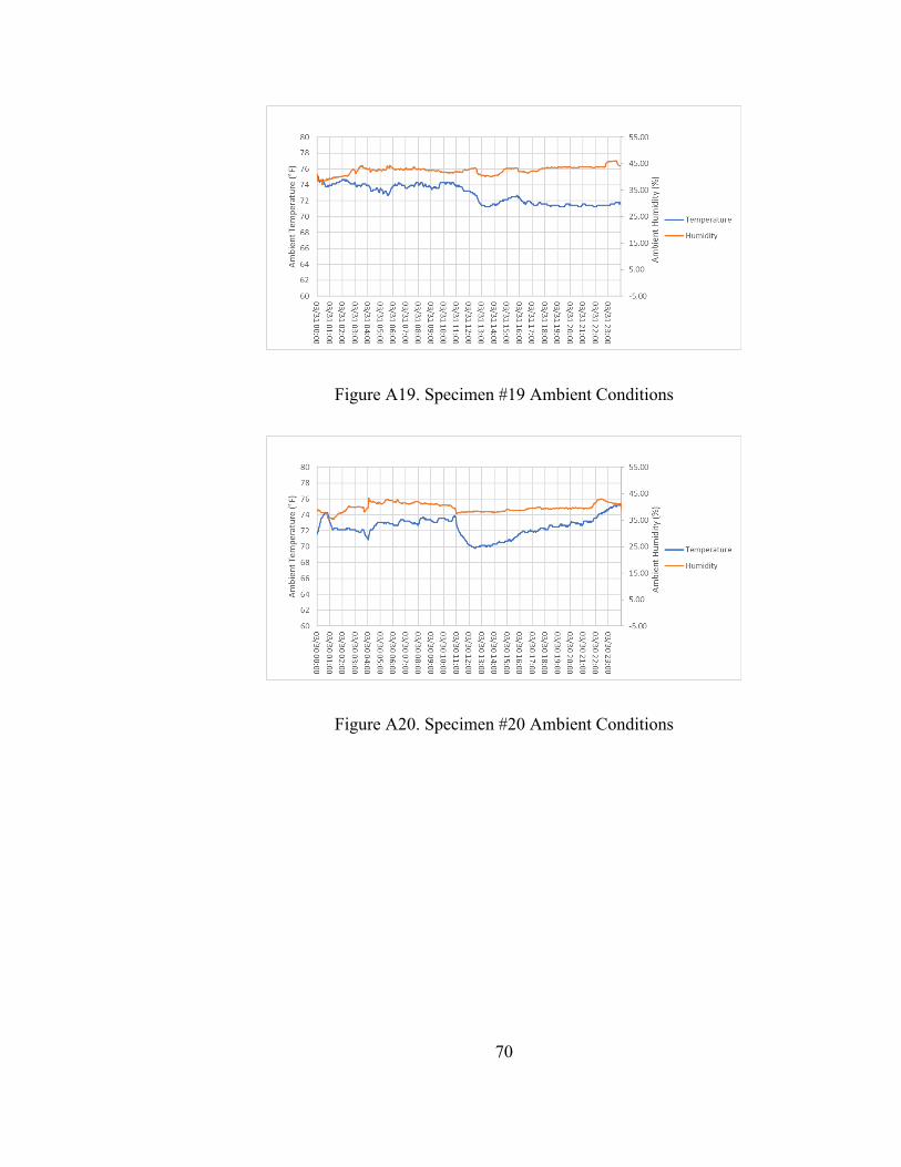
Temperature and Humidity
To monitor the ambient temperature and humidity during printing, a Raspberry Pi
3B+ was used in conjunction with a DHT22 temperature and humidity sensor. The
DHT22 was connected to the GPIO pins on the Raspberry Pi 3B+ and the data were
collected using a custom code and sent to the data visualization tool initial state via wifi.
Data were recorded in real time and downloaded into Excel for analysis and visualization.
In order to run the custom program a second Raspberry Pi zero w was used to Secure
Shell Protocol into the first Raspberry Pi 3B+ and run the program. The Raspberry Pi
zero w acted as a control point to initialize the code and start sending data to initial state.
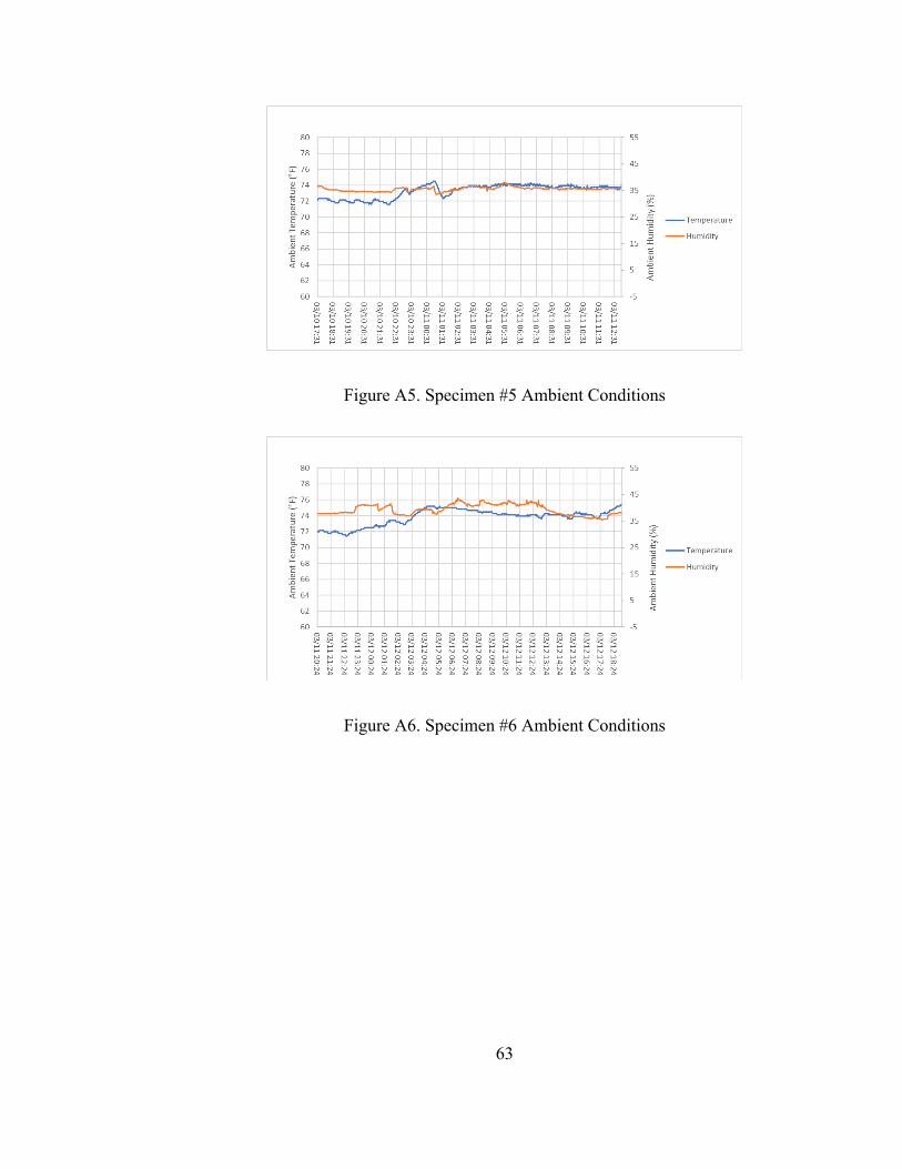
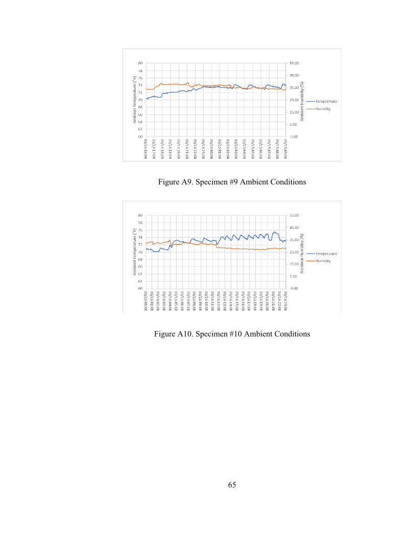
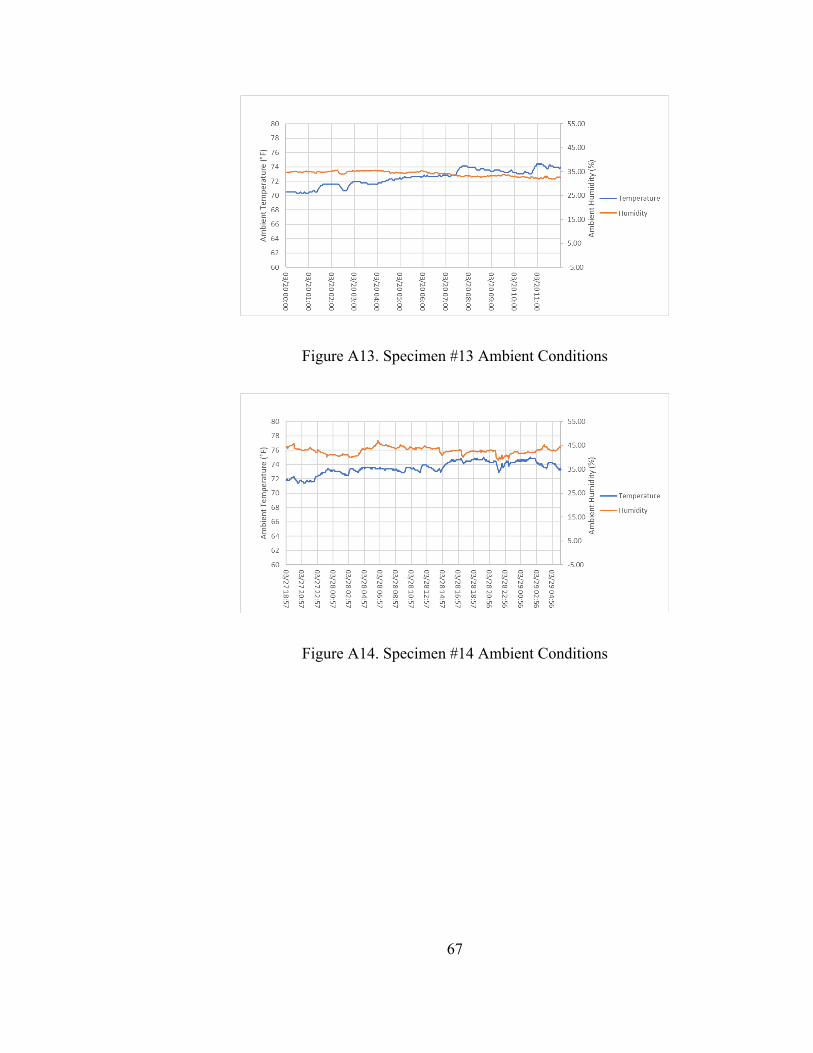
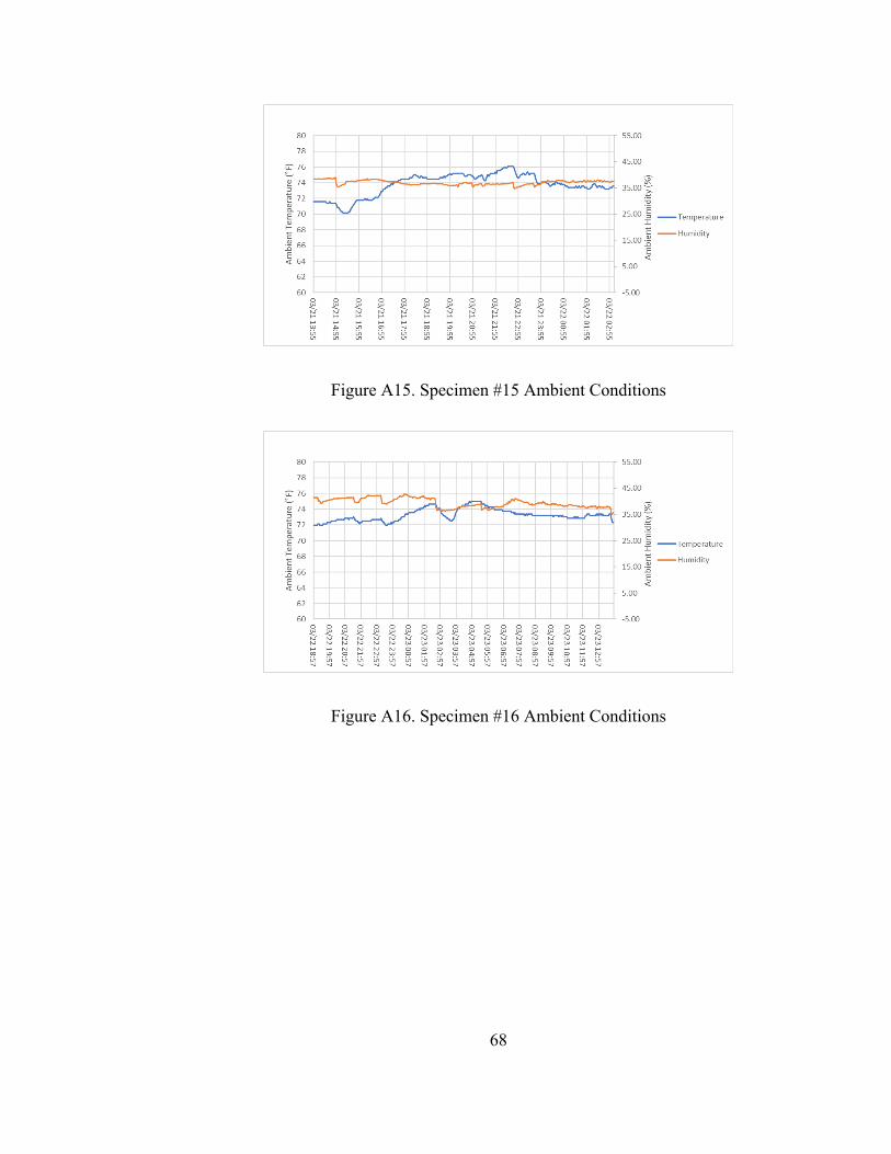
An example of the formatted graph is shown in Figure 28.
Figure 28. Exemplar temperature and humidity graph from Run 1.
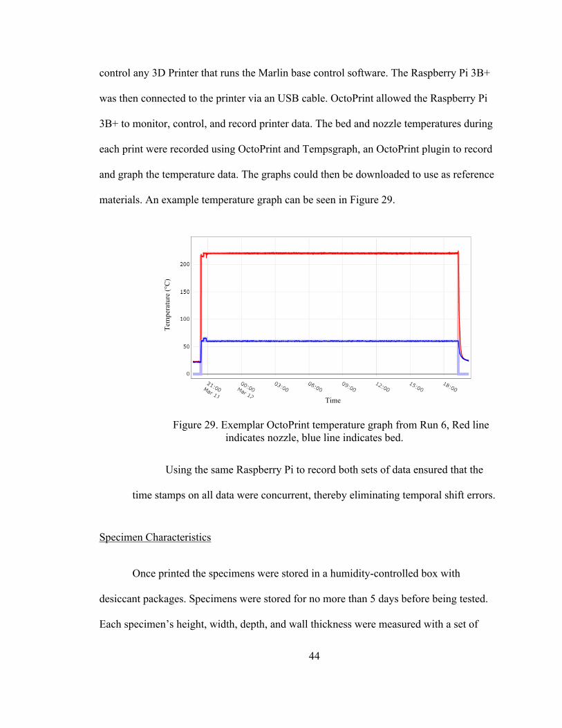
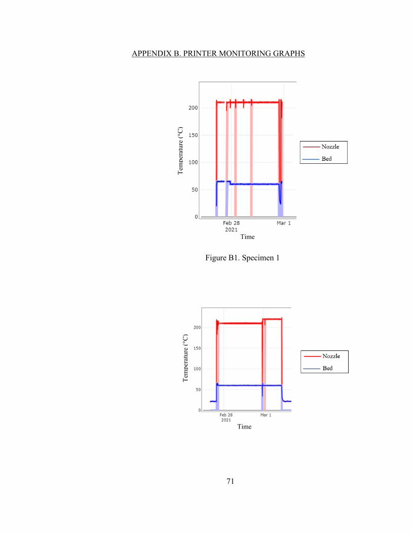
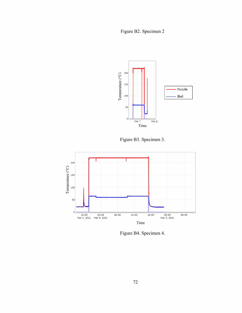
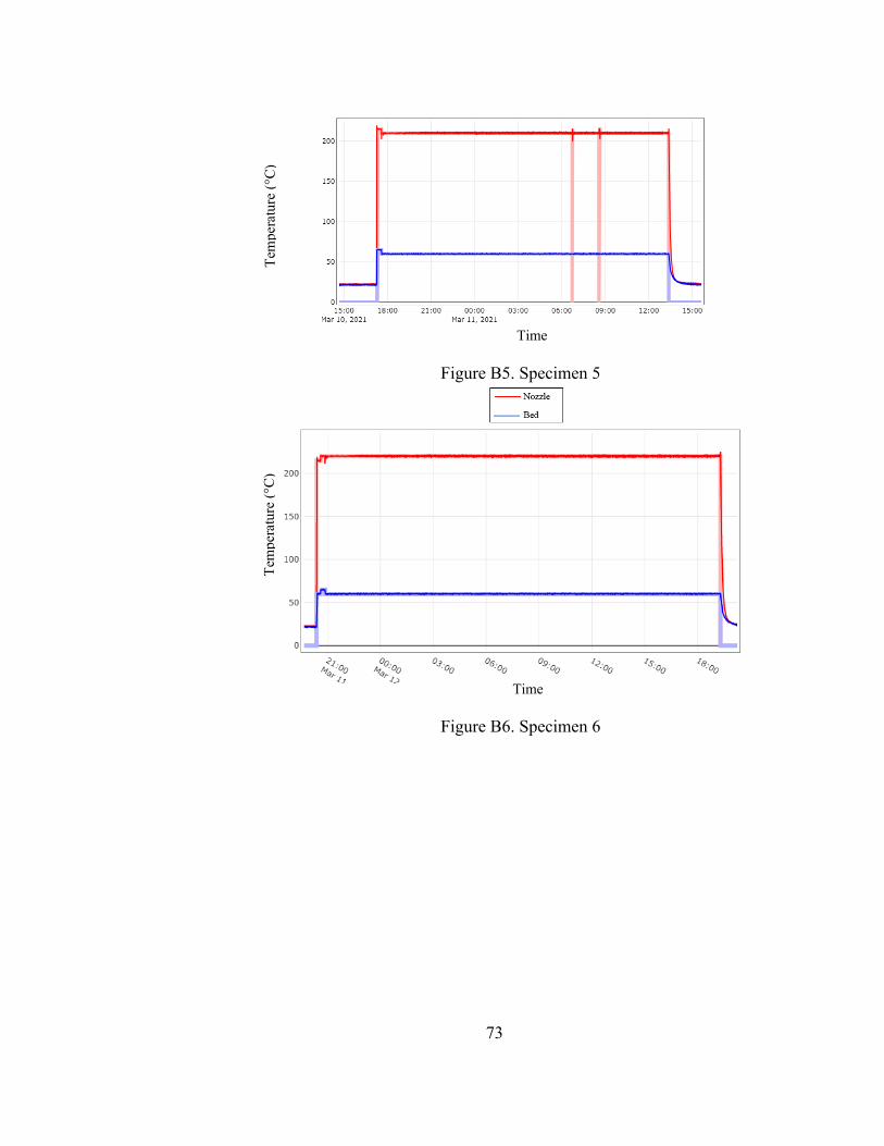
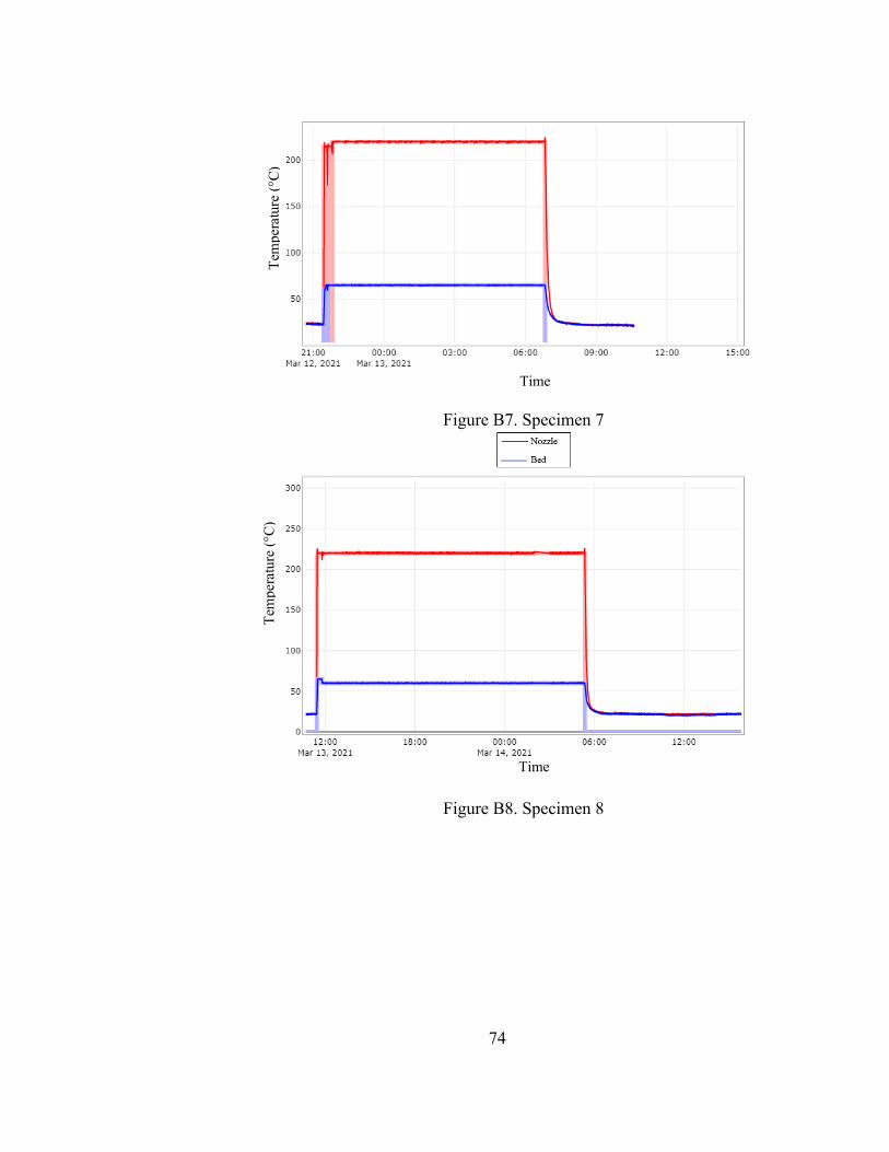
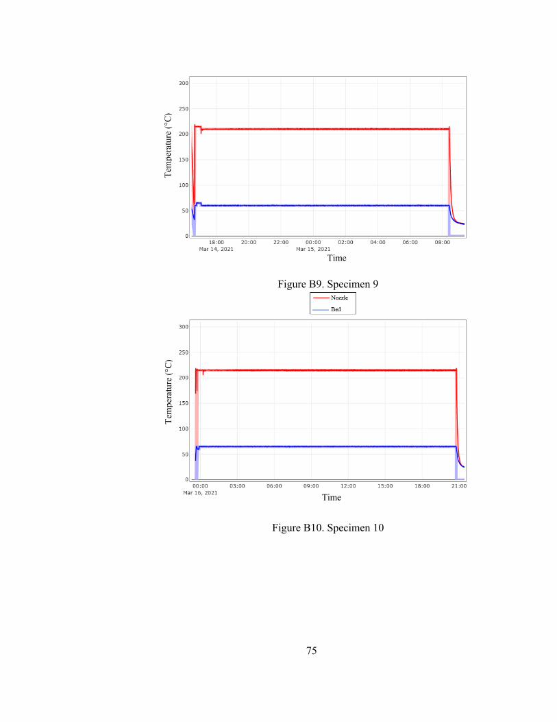
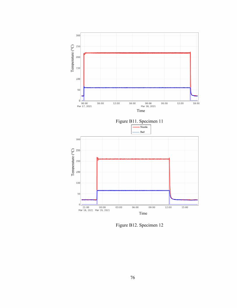
In order to collect data on the printer such as nozzle and bed temperature, the
Raspberry Pi 3B+ was configured to run OctoPrint, a program to remotely monitor and
44
control any 3D Printer that runs the Marlin base control software. The Raspberry Pi 3B+
was then connected to the printer via an USB cable. OctoPrint allowed the Raspberry Pi
3B+ to monitor, control, and record printer data. The bed and nozzle temperatures during
each print were recorded using OctoPrint and Tempsgraph, an OctoPrint plugin to record
and graph the temperature data. The graphs could then be downloaded to use as reference
materials. An example temperature graph can be seen in Figure 29.
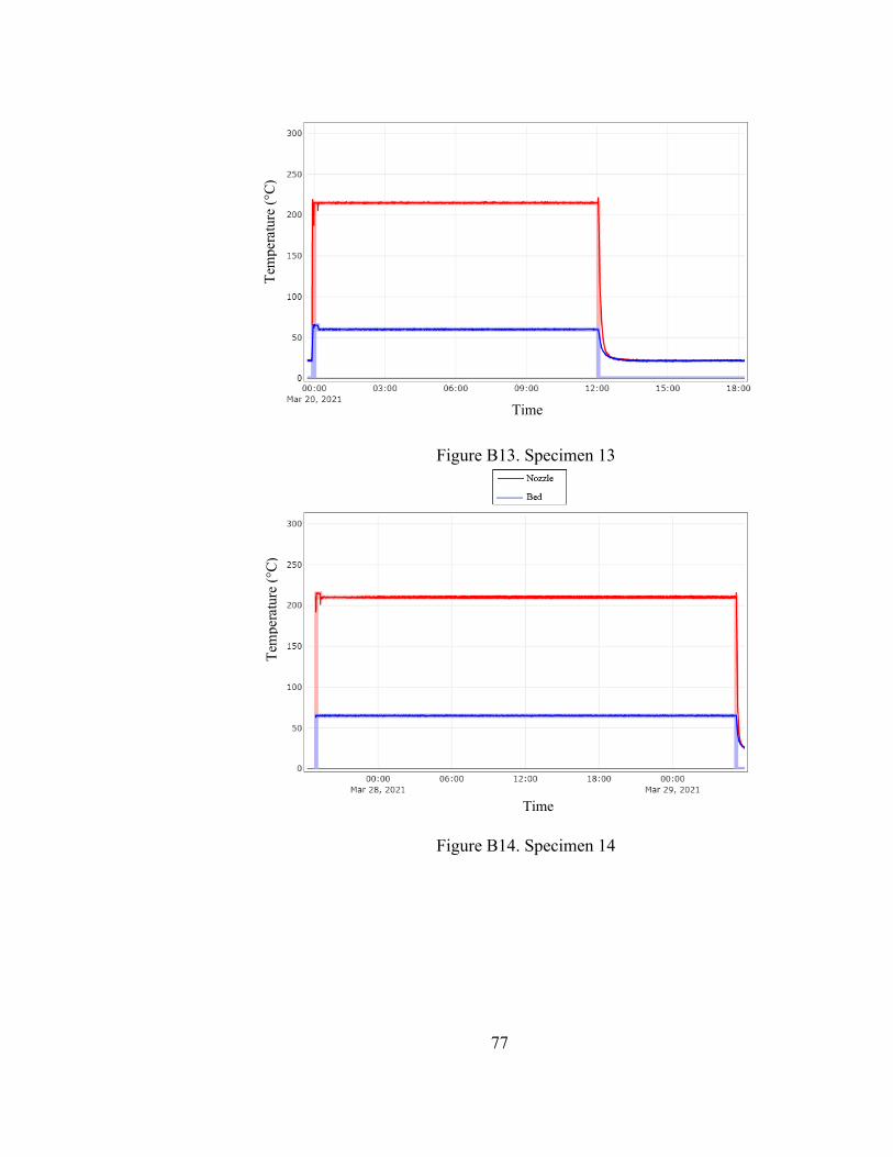
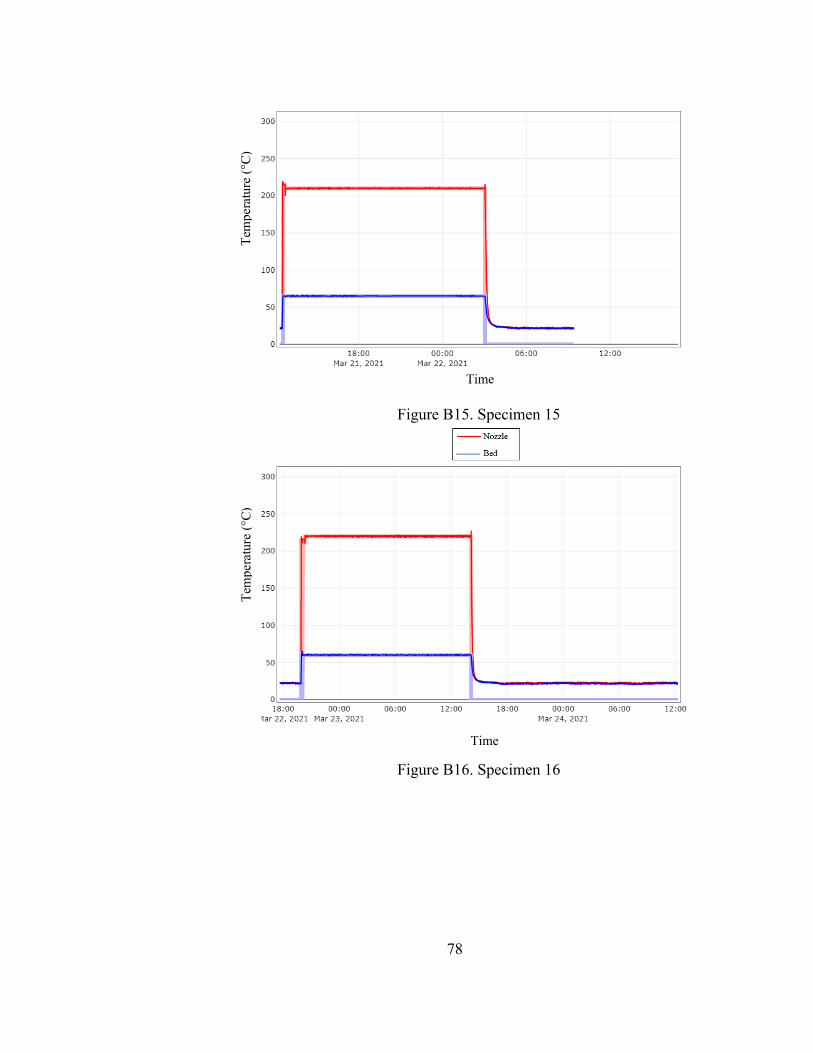
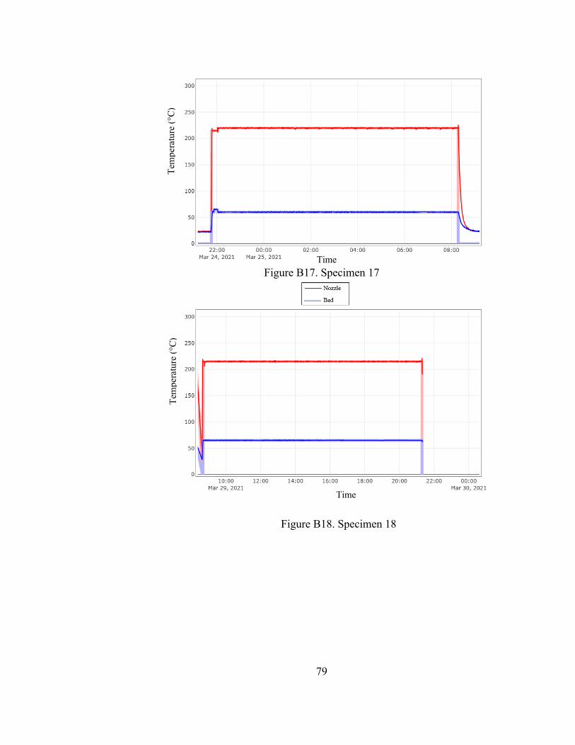
Figure 29. Exemplar OctoPrint temperature graph from Run 6, Red line indicates nozzle, blue line indicates bed.
Using the same Raspberry Pi to record both sets of data ensured that the
time stamps on all data were concurrent, thereby eliminating temporal shift errors.
Specimen Characteristics
Once printed the specimens were stored in a humidity-controlled box with
desiccant packages. Specimens were stored for no more than 5 days before being tested.
Each specimen’s height, width, depth, and wall thickness were measured with a set of
Time
Tem
pera
ture
(°C
)
45
General Stainless-Steel digital calipers. Width, depth, and wall thickness were measured
in triplicate, which were utilized to calculate average width, depth, and thickness.
Calipers were also utilized to measure a single height measurement for each specimen.
The mass of each specimen was recorded using a CEN-TECH digital scale.
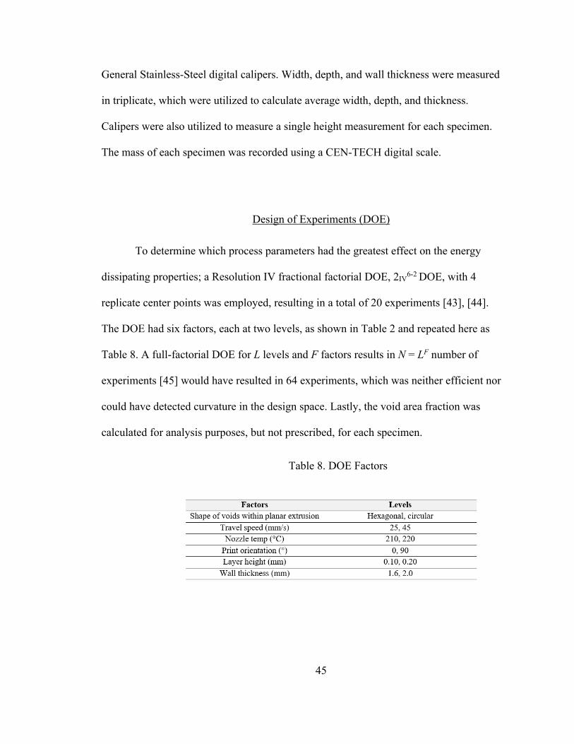
Design of Experiments (DOE)
To determine which process parameters had the greatest effect on the energy
dissipating properties; a Resolution IV fractional factorial DOE, 2IV6-2 DOE, with 4
replicate center points was employed, resulting in a total of 20 experiments [43], [44].
The DOE had six factors, each at two levels, as shown in Table 2 and repeated here as
Table 8. A full-factorial DOE for L levels and F factors results in N = LF number of
experiments [45] would have resulted in 64 experiments, which was neither efficient nor
could have detected curvature in the design space. Lastly, the void area fraction was
calculated for analysis purposes, but not prescribed, for each specimen.
Table 8. DOE Factors

46
CHAPTER III: RESULTS AND ANALYSIS
The data was entered into Minitab as described in Chapter II. The program
resulted in 20 different specimens with various combinations of factors. The composition
of each specimen can be seen in Table 9.
Table 9. Specimens showing shape of void, travel speed, nozzle temp, print orientation, layer height and wall thickness DOE factors and levels.
After printing, specimens were measured and tested as described in Chapter II.
Height, width, depth, wall thickness, and mass measurement results for each specimen
are showed in Table 10.
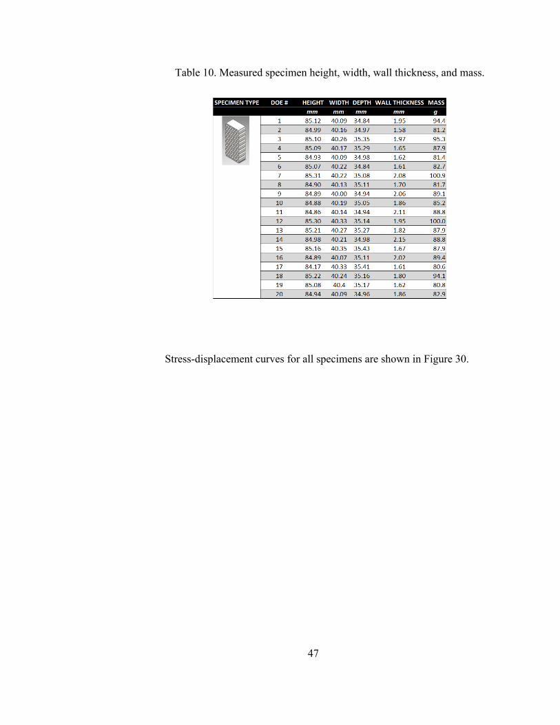
47
Table 10. Measured specimen height, width, wall thickness, and mass.
Stress-displacement curves for all specimens are shown in Figure 30.
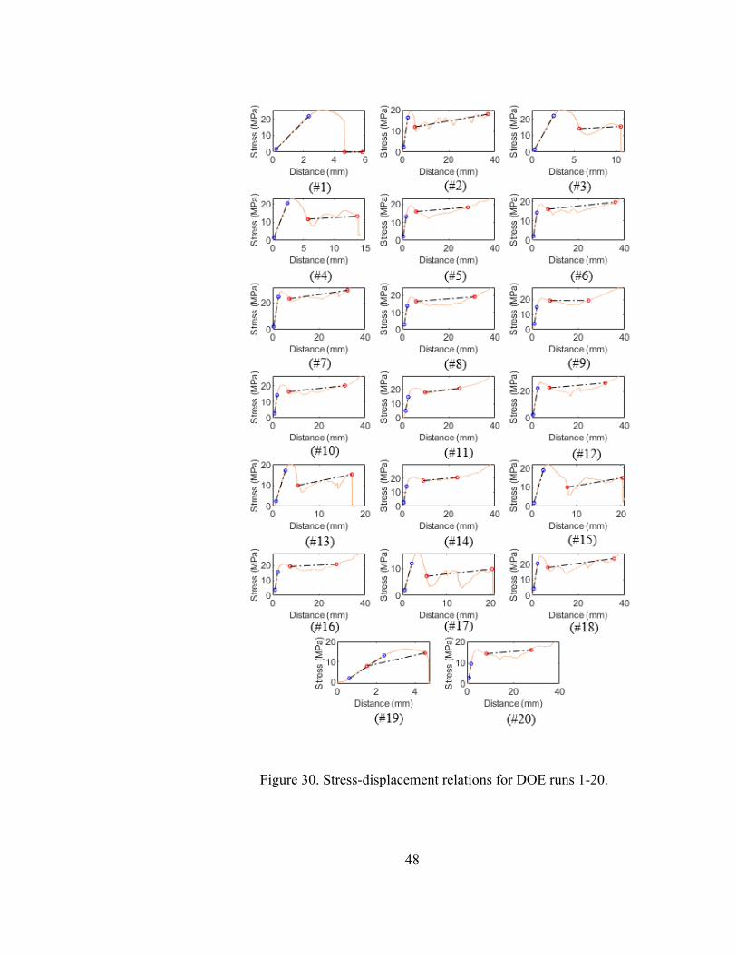
48
Figure 30. Stress-displacement relations for DOE runs 1-20.
49
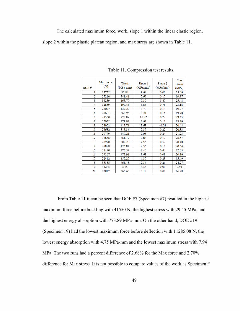
The calculated maximum force, work, slope 1 within the linear elastic region,
slope 2 within the plastic plateau region, and max stress are shown in Table 11.
Table 11. Compression test results.
From Table 11 it can be seen that DOE #7 (Specimen #7) resulted in the highest
maximum force before buckling with 41550 N, the highest stress with 29.45 MPa, and
the highest energy absorption with 773.89 MPa-mm. On the other hand, DOE #19
(Specimen 19) had the lowest maximum force before deflection with 11285.08 N, the
lowest energy absorption with 4.75 MPa-mm and the lowest maximum stress with 7.94
MPa. The two runs had a percent difference of 2.68% for the Max force and 2.70%
difference for Max stress. It is not possible to compare values of the work as Specimen #
50
19 failed prematurely and could not be tested completely. DOE #1,3,4,13,15,17, and 19
all failed prematurely and could not be tested for the full 500 seconds as described in
Chapter II. The specimens failed at different points with the main cause of failure being
geometry of the specimens.
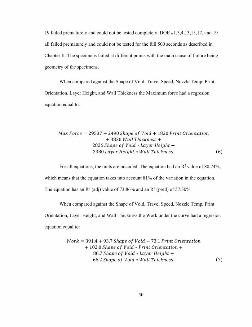
When compared against the Shape of Void, Travel Speed, Nozzle Temp, Print
Orientation, Layer Height, and Wall Thickness the Maximum force had a regresion
equation equal to:
𝑀𝑎𝑥𝐹𝑜𝑟𝑐𝑒 = 29537 + 2490𝑆ℎ𝑎𝑝𝑒𝑜𝑓𝑉𝑜𝑖𝑑 + 1820𝑃𝑟𝑖𝑛𝑡𝑂𝑟𝑖𝑒𝑛𝑡𝑎𝑡𝑖𝑜𝑛+3820𝑊𝑎𝑙𝑙𝑇ℎ𝑖𝑐𝑘𝑛𝑒𝑠𝑠 +
2826𝑆ℎ𝑎𝑝𝑒𝑜𝑓𝑉𝑜𝑖𝑑 ∗ 𝐿𝑎𝑦𝑒𝑟𝐻𝑒𝑖𝑔ℎ𝑡 +2380𝐿𝑎𝑦𝑒𝑟𝐻𝑒𝑖𝑔ℎ𝑡 ∗ 𝑊𝑎𝑙𝑙𝑇ℎ𝑖𝑐𝑘𝑛𝑒𝑠𝑠 (6)
For all equations, the units are uncoded. The equation had an R2 value of 80.74%,
which means that the equation takes into account 81% of the variation in the equation.
The equation has an R2 (adj) value of 73.86% and an R2 (pred) of 57.30%.
When compared against the Shape of Void, Travel Speed, Nozzle Temp, Print
Orientation, Layer Height, and Wall Thickness the Work under the curve had a regresion
equation equal to:
𝑊𝑜𝑟𝑘 = 391.4 + 93.7𝑆ℎ𝑎𝑝𝑒𝑜𝑓𝑉𝑜𝑖𝑑 − 73.1𝑃𝑟𝑖𝑛𝑡𝑂𝑟𝑖𝑒𝑛𝑡𝑎𝑡𝑖𝑜𝑛+102.0𝑆ℎ𝑎𝑝𝑒𝑜𝑓𝑉𝑜𝑖𝑑 ∗ 𝑃𝑟𝑖𝑛𝑡𝑂𝑟𝑖𝑒𝑛𝑡𝑎𝑡𝑖𝑜𝑛 +
80.7𝑆ℎ𝑎𝑝𝑒𝑜𝑓𝑉𝑜𝑖𝑑 ∗ 𝐿𝑎𝑦𝑒𝑟𝐻𝑒𝑖𝑔ℎ𝑡 +66.2𝑆ℎ𝑎𝑝𝑒𝑜𝑓𝑉𝑜𝑖𝑑 ∗ 𝑊𝑎𝑙𝑙𝑇ℎ𝑖𝑐𝑘𝑛𝑒𝑠𝑠 (7)
51
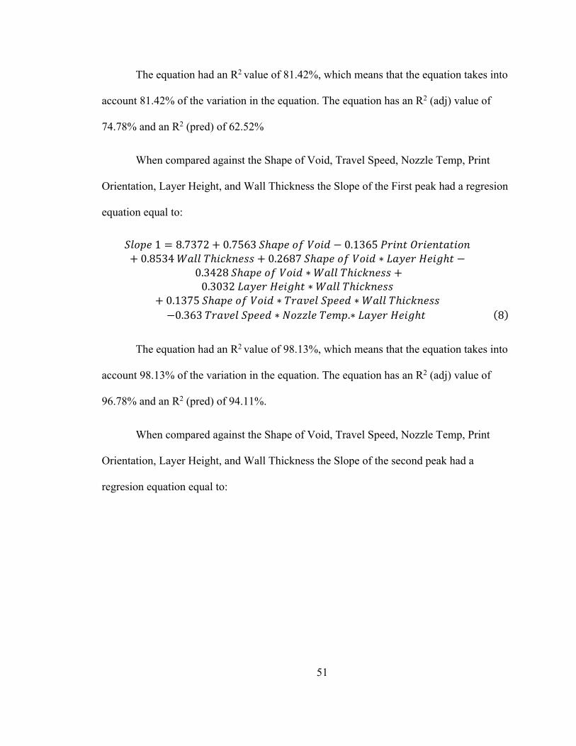
The equation had an R2 value of 81.42%, which means that the equation takes into
account 81.42% of the variation in the equation. The equation has an R2 (adj) value of
74.78% and an R2 (pred) of 62.52%
When compared against the Shape of Void, Travel Speed, Nozzle Temp, Print
Orientation, Layer Height, and Wall Thickness the Slope of the First peak had a regresion
equation equal to:
𝑆𝑙𝑜𝑝𝑒1 = 8.7372 + 0.7563𝑆ℎ𝑎𝑝𝑒𝑜𝑓𝑉𝑜𝑖𝑑 − 0.1365𝑃𝑟𝑖𝑛𝑡𝑂𝑟𝑖𝑒𝑛𝑡𝑎𝑡𝑖𝑜𝑛+0.8534𝑊𝑎𝑙𝑙𝑇ℎ𝑖𝑐𝑘𝑛𝑒𝑠𝑠 + 0.2687𝑆ℎ𝑎𝑝𝑒𝑜𝑓𝑉𝑜𝑖𝑑 ∗ 𝐿𝑎𝑦𝑒𝑟𝐻𝑒𝑖𝑔ℎ𝑡 −
0.3428𝑆ℎ𝑎𝑝𝑒𝑜𝑓𝑉𝑜𝑖𝑑 ∗ 𝑊𝑎𝑙𝑙𝑇ℎ𝑖𝑐𝑘𝑛𝑒𝑠𝑠 +0.3032𝐿𝑎𝑦𝑒𝑟𝐻𝑒𝑖𝑔ℎ𝑡 ∗ 𝑊𝑎𝑙𝑙𝑇ℎ𝑖𝑐𝑘𝑛𝑒𝑠𝑠
+0.1375𝑆ℎ𝑎𝑝𝑒𝑜𝑓𝑉𝑜𝑖𝑑 ∗ 𝑇𝑟𝑎𝑣𝑒𝑙𝑆𝑝𝑒𝑒𝑑 ∗ 𝑊𝑎𝑙𝑙𝑇ℎ𝑖𝑐𝑘𝑛𝑒𝑠𝑠−0.363𝑇𝑟𝑎𝑣𝑒𝑙𝑆𝑝𝑒𝑒𝑑 ∗ 𝑁𝑜𝑧𝑧𝑙𝑒𝑇𝑒𝑚𝑝.∗ 𝐿𝑎𝑦𝑒𝑟𝐻𝑒𝑖𝑔ℎ𝑡 (8)
The equation had an R2 value of 98.13%, which means that the equation takes into
account 98.13% of the variation in the equation. The equation has an R2 (adj) value of
96.78% and an R2 (pred) of 94.11%.
When compared against the Shape of Void, Travel Speed, Nozzle Temp, Print
Orientation, Layer Height, and Wall Thickness the Slope of the second peak had a
regresion equation equal to:
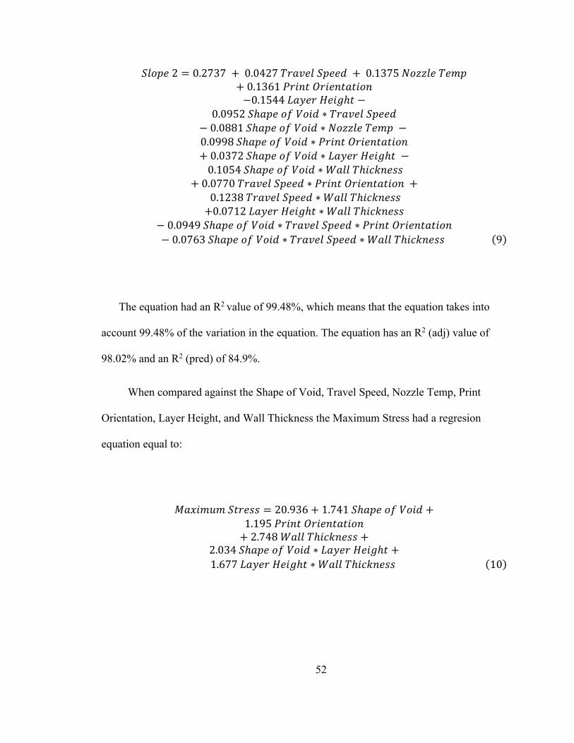
52
𝑆𝑙𝑜𝑝𝑒2 = 0.2737 + 0.0427𝑇𝑟𝑎𝑣𝑒𝑙𝑆𝑝𝑒𝑒𝑑 + 0.1375𝑁𝑜𝑧𝑧𝑙𝑒𝑇𝑒𝑚𝑝+0.1361𝑃𝑟𝑖𝑛𝑡𝑂𝑟𝑖𝑒𝑛𝑡𝑎𝑡𝑖𝑜𝑛−0.1544𝐿𝑎𝑦𝑒𝑟𝐻𝑒𝑖𝑔ℎ𝑡 −
0.0952𝑆ℎ𝑎𝑝𝑒𝑜𝑓𝑉𝑜𝑖𝑑 ∗ 𝑇𝑟𝑎𝑣𝑒𝑙𝑆𝑝𝑒𝑒𝑑−0.0881𝑆ℎ𝑎𝑝𝑒𝑜𝑓𝑉𝑜𝑖𝑑 ∗ 𝑁𝑜𝑧𝑧𝑙𝑒𝑇𝑒𝑚𝑝 −0.0998𝑆ℎ𝑎𝑝𝑒𝑜𝑓𝑉𝑜𝑖𝑑 ∗ 𝑃𝑟𝑖𝑛𝑡𝑂𝑟𝑖𝑒𝑛𝑡𝑎𝑡𝑖𝑜𝑛+0.0372𝑆ℎ𝑎𝑝𝑒𝑜𝑓𝑉𝑜𝑖𝑑 ∗ 𝐿𝑎𝑦𝑒𝑟𝐻𝑒𝑖𝑔ℎ𝑡 −0.1054𝑆ℎ𝑎𝑝𝑒𝑜𝑓𝑉𝑜𝑖𝑑 ∗ 𝑊𝑎𝑙𝑙𝑇ℎ𝑖𝑐𝑘𝑛𝑒𝑠𝑠
+0.0770𝑇𝑟𝑎𝑣𝑒𝑙𝑆𝑝𝑒𝑒𝑑 ∗ 𝑃𝑟𝑖𝑛𝑡𝑂𝑟𝑖𝑒𝑛𝑡𝑎𝑡𝑖𝑜𝑛 +0.1238𝑇𝑟𝑎𝑣𝑒𝑙𝑆𝑝𝑒𝑒𝑑 ∗ 𝑊𝑎𝑙𝑙𝑇ℎ𝑖𝑐𝑘𝑛𝑒𝑠𝑠+0.0712𝐿𝑎𝑦𝑒𝑟𝐻𝑒𝑖𝑔ℎ𝑡 ∗ 𝑊𝑎𝑙𝑙𝑇ℎ𝑖𝑐𝑘𝑛𝑒𝑠𝑠
−0.0949𝑆ℎ𝑎𝑝𝑒𝑜𝑓𝑉𝑜𝑖𝑑 ∗ 𝑇𝑟𝑎𝑣𝑒𝑙𝑆𝑝𝑒𝑒𝑑 ∗ 𝑃𝑟𝑖𝑛𝑡𝑂𝑟𝑖𝑒𝑛𝑡𝑎𝑡𝑖𝑜𝑛−0.0763𝑆ℎ𝑎𝑝𝑒𝑜𝑓𝑉𝑜𝑖𝑑 ∗ 𝑇𝑟𝑎𝑣𝑒𝑙𝑆𝑝𝑒𝑒𝑑 ∗ 𝑊𝑎𝑙𝑙𝑇ℎ𝑖𝑐𝑘𝑛𝑒𝑠𝑠 (9)
The equation had an R2 value of 99.48%, which means that the equation takes into
account 99.48% of the variation in the equation. The equation has an R2 (adj) value of
98.02% and an R2 (pred) of 84.9%.
When compared against the Shape of Void, Travel Speed, Nozzle Temp, Print
Orientation, Layer Height, and Wall Thickness the Maximum Stress had a regresion
equation equal to:
𝑀𝑎𝑥𝑖𝑚𝑢𝑚𝑆𝑡𝑟𝑒𝑠𝑠 = 20.936 + 1.741𝑆ℎ𝑎𝑝𝑒𝑜𝑓𝑉𝑜𝑖𝑑 +1.195𝑃𝑟𝑖𝑛𝑡𝑂𝑟𝑖𝑒𝑛𝑡𝑎𝑡𝑖𝑜𝑛+2.748𝑊𝑎𝑙𝑙𝑇ℎ𝑖𝑐𝑘𝑛𝑒𝑠𝑠 +
2.034𝑆ℎ𝑎𝑝𝑒𝑜𝑓𝑉𝑜𝑖𝑑 ∗ 𝐿𝑎𝑦𝑒𝑟𝐻𝑒𝑖𝑔ℎ𝑡 +1.677𝐿𝑎𝑦𝑒𝑟𝐻𝑒𝑖𝑔ℎ𝑡 ∗ 𝑊𝑎𝑙𝑙𝑇ℎ𝑖𝑐𝑘𝑛𝑒𝑠𝑠 (10)

53
The equation had an R2 value of 80.73%, which means that the equation takes into
account 80.73% of the variation in the equation. The equation has an R2 (adj) value of
73.85% and an R2 (pred) of 57.33%.
54
CHAPTER IV: CONCLUSIONS
The aim of this research was to quantify the effects of meso structure and process
parameters on energy dissipative properties of additively manufactured regular hexagonal
honeycomb structures. The research included manufacturing, compressive testing, and
analyzing 20 different specimens within a fractional factorial Design of Experiments
(DOE) framework. The six factors within the DOE were shape of voids [hexagonal,
circular], travel speed [25, 45 mm/s], nozzle temperature [210, 220 ℃], print orientation
[0°, 90°], layer height [0.10, 0.20 mm], and wall thickness [1.6, 2.0 mm]. The 20
specimens were then 3D printed and tested on an MTS load frame. The results were
analyzed using MATLAB and Minitab. The results showed a correlation between the
process parameters and meso structure and the energy dissipative properties of the
specimens.
From the actual specimen results it can be readily concluded that PLA is a
suitable material for buckling applications when the material is properly used and stored
to prevent environmental degradation. It was observed on multiple occasions that the
PLA specimen buckled as would be expected of its aluminum or metal counterparts.
From the results of the DOE, it was determined that when the specimen was to
handle the most initial force or stress, the factor that impacted this the most was the wall
thickness for the factors and levels considered. It was concluded that as the wall thickness
increased the maximum force increased. For maximum force it was also noted that the
55
combination of Shape of Void and Layer height had the second greatest effect for the
factors and levels considered. The factor that effected the maximum force the least was
the print orientation. What this means is that when designing for maximum force the print
should be oriented to save time and money on material.
From the DOE, it was determined that when designing for the highest energy
absorption the designer should focus upon the combination of the Shape of the Void and
the Print orientation as the combination of these two factors had the greatest effect upon
the factors and levels considered. The combination of Shape of Void and Wall thickness
had the least effect upon energy absorption given the factors and levels considered.
From the same round of results of the DOE, it was determined that when
designing for the highest initial modulus of elasticity (slope of initial curve) that the
designer should focus on the wall thickness as this had the greatest effect for the factors
and levels considered. The analysis also revealed that a combination of shape of void,
travel speed, and wall thickness contributed the least given the factors and levels
considered.
The DOE results also indicated that the slope of the remaining peaks (average)
was most effected by layer height given the factors and levels considered. The smaller the
layer height the smaller the average slope was found to be. A combination of Layer
height and wall thickness affected the second slope the least against factors and levels
considered.

56
REFERENCES
[1] US DOT Federal Highway Administration, “How Do Weather Events Impact Roads.” https://ops.fhwa.dot.gov/weather/q1_roadimpact.htm (accessed Oct. 22, 2020).
[2] B. P. DiPaolo and J. G. Tom, “A study on an axial crush configuration response of thin-wall, steel box components: The quasi-static experiments,” Int. J. Solids Struct., vol. 43, no. 25, pp. 7752–7775, Dec. 2006, doi: 10.1016/j.ijsolstr.2006.03.028.
[3] “How Can 3D Optical Profiling Optimize Additive Manufacturing Processes?,” AZoM.com, Apr. 17, 2019. https://www.azom.com/article.aspx?ArticleID=17901 (accessed Mar. 28, 2021).
[4] Brett Ellis, “MET 320: Additive Manufacturing Lecture 2: History & Processes,” University of Maine, Orono, Jan. 27, 2020.
[5] “Source Rabbit launches desktop CNC milling machine.” http://www.gizmoeditor.com/2019/11/source-rabbit-launches-desktop-cnc.html (accessed Mar. 28, 2021).
[6] “The History of 3D Printing: From the 80s to Today,” Sculpteo. https://www.sculpteo.com/en/3d-learning-hub/basics-of-3d-printing/the-history-of-3d-printing/ (accessed Mar. 28, 2021).
[7] “NIHF Inductee Charles Hull, Who Invented the 3D Printer.” https://www.invent.org/inductees/charles-hull (accessed Mar. 28, 2021).
[8] T. Wohlers and T. Gornet, “History of additive manufacturing,” p. 38, 2016.
[9] “GENISYS XS.” http://www.cs.cmu.edu/~rapidproto/students.00/reginaw/Project2/GENISYS%20XS.htm (accessed Mar. 28, 2021).
[10] “About Josef Prusa and Prusa Research,” Prusa3D - 3D Printers from Josef Průša. https://www.prusa3d.com/about-us/ (accessed Mar. 28, 2021).
[11] “Original Prusa i3 MK3S + - Prusa Research.” https://shop.prusa3d.com/de/51-original-prusa-i3-mk3s (accessed Mar. 28, 2021).
[12] B. M. Tymrak, M. Kreiger, and J. M. Pearce, “Mechanical properties of components fabricated with open-source 3-D printers under realistic environmental conditions,” Mater. Des., vol. 58, pp. 242–246, Jun. 2014, doi: 10.1016/j.matdes.2014.02.038.
[13] T. Letcher and M. Waytashek, “Material Property Testing of 3D-Printed Specimen in PLA on an Entry-Level 3D Printer,” Dec. 2014, vol. 2. doi: 10.1115/IMECE2014-39379.
57
[14] T. Yao, Z. Deng, K. Zhang, and S. Li, “A method to predict the ultimate tensile strength of 3D printing polylactic acid (PLA) materials with different printing orientations,” Compos. Part B Eng., vol. 163, pp. 393–402, Apr. 2019, doi: 10.1016/j.compositesb.2019.01.025.
[15] “Table 3 : Material Properties of PLA and ABS [22] [23],” ResearchGate. https://www.researchgate.net/figure/Material-Properties-of-PLA-and-ABS-22-23_tbl1_319489894 (accessed May 03, 2021).
[16] S. says, “Is PLA filament actually biodegradable?,” 3Dnatives, Jul. 23, 2019. https://www.3dnatives.com/en/pla-filament-230720194/ (accessed Apr. 13, 2021).
[17] J. S. Dugan, “Novel Properties of PLA Fibers,” Int. Nonwovens J., vol. os-10, no. 3, pp. 1558925001OS–01000308, Sep. 2001, doi: 10.1177/1558925001OS-01000308.
[18] matweb, “Overview of materials for Polylactic Acid (PLA) Biopolymer.” http://www.matweb.com/search/DataSheet.aspx?MatGUID=ab96a4c0655c4018a8785ac4031b9278&ckck=1 (accessed Oct. 22, 2020).
[19] “ABS vs PLA: Everything You Need To Know About The Two Most Popular 3D Printing Filaments – Geeetech Blog.” https://www.geeetech.com/blog/2017/12/abs-vs-pla-everything-you-need-to-know-about-the-two-most-popular-3d-printing-filaments/ (accessed May 03, 2021).
[20] “Amazon.com: HATCHBOX PLA 3D Printer Filament, Dimensional Accuracy +/- 0.03 mm, 1 kg Spool, 1.75 mm, White: Industrial & Scientific.” https://www.amazon.com/HATCHBOX-3D-Filament-Dimensional-Accuracy/dp/B00J0GMMP6?ref_=fsclp_pl_dp_1 (accessed Aug. 11, 2020).
[21] Prusa Research, “Prusament PLA Jet Black 1kg,” Prusa Research. https://shop.prusa3d.com/en/prusament/959-prusament-pla-jet-black-1kg.html (accessed Aug. 11, 2020).
[22] G. B. Olson, “Computational Design of Hierarchically Structured Materials,” Science, vol. 277, no. 5330, pp. 1237–1242, Aug. 1997, doi: 10.1126/science.277.5330.1237.
[23] Donals R. Askeland and Wendelin J. Wright, Essentials of Materials Science and Engineering, 4th ed. Cengage, 2019.
[24] T. J. Coogan and D. O. Kazmer, “Prediction of interlayer strength in material extrusion additive manufacturing,” Addit. Manuf., vol. 35, p. 101368, Oct. 2020, doi: 10.1016/j.addma.2020.101368.
[25] J. Torres, M. Cole, A. Owji, Z. DeMastry, and A. P. Gordon, “An approach for mechanical property optimization of fused deposition modeling with polylactic
58
acid via design of experiments,” Rapid Prototyp. J., vol. 22, no. 2, pp. 387–404, Jan. 2016, doi: 10.1108/RPJ-07-2014-0083.
[26] A. Tsouknidas, M. Pantazopoulos, I. Katsoulis, D. Fasnakis, S. Maropoulos, and N. Michailidis, “Impact absorption capacity of 3D-printed components fabricated by fused deposition modelling,” Mater. Des., vol. 102, pp. 41–44, Jul. 2016, doi: 10.1016/j.matdes.2016.03.154.
[27] Y. Chen, T. Li, Z. Jia, F. Scarpa, C.-W. Yao, and L. Wang, “3D printed hierarchical honeycombs with shape integrity under large compressive deformations,” Mater. Des., vol. 137, pp. 226–234, Jan. 2018, doi: 10.1016/j.matdes.2017.10.028.
[28] E. R. Braver, A. T. McCartt, C. P. Sherwood, D. S. Zuby, L. Blanar, and M. Scerbo, “Front air bag nondeployments in frontal crashes fatal to drivers or right-front passengers,” Traffic Inj. Prev., vol. 11, no. 2, pp. 178–187, Apr. 2010, doi: 10.1080/15389580903473973.
[29] P. D. Bois et al., Vehicle Crashworthiness and Occupant Protection. American Iron and Steel Institute, 2004.
[30] M. Altin, S. Halis, and H. Serdar Yücesu, “Investigation of the effect of corrugated structure on crashing performance in thin-walled circular tubes,” Int. J. Automot. Sci. Technol., vol. 1, no. 2, pp. 1–7, Mar. 2017.
[31] K. Yang, S. Xu, J. Shen, S. Zhou, and Y. M. Xie, “Energy absorption of thin-walled tubes with pre-folded origami patterns: Numerical simulation and experimental verification,” Thin-Walled Struct., vol. 103, pp. 33–44, Jun. 2016, doi: 10.1016/j.tws.2016.02.007.
[32] M. R. Bambach, “Fibre composite strengthening of thin-walled steel vehicle crush tubes for frontal collision energy absorption,” Thin-Walled Struct., vol. 66, pp. 15–22, May 2013, doi: 10.1016/j.tws.2013.02.006.
[33] S. K. Subramaniyan, A. Kananasan, M. Yunus, S. Mahzan, and M. I. Ghazali, “Crush Characteristics and Energy Absorption of Thin-Walled Tubes with Through-Hole Crush Initiators,” Appl. Mech. Mater., vol. 606, pp. 181–185, Aug. 2014, doi: 10.4028/www.scientific.net/AMM.606.181.
[34] L. J. Gibson and M. F. Ashby, Cellular Solids- Structure and properties, 2nd ed. Press Syndicate of The University of Cambridge, 1997.
[35] Q. Zhang et al., “Bioinspired engineering of honeycomb structure – Using nature to inspire human innovation,” Prog. Mater. Sci., vol. 74, pp. 332–400, Oct. 2015, doi: 10.1016/j.pmatsci.2015.05.001.
[36] Y. L. Yap and W. Y. Yeong, “Shape recovery effect of 3D printed polymeric honeycomb,” Virtual Phys. Prototyp., vol. 10, pp. 91–99, Apr. 2015, doi: 10.1080/17452759.2015.1060350.
59
[37] Dassault Systèmes, Solidworks Educational Edition 2019-2020. San Diego: Dassault Systèmes, 2020.
[38] “PrusaSlicer - Prusa3d.com - 3D printers by Josef Prusa,” Prusa3D - 3D Printers from Josef Průša. https://www.prusa3d.com/prusaslicer/ (accessed Apr. 25, 2021).
[39] Prusa Polymers, “Technical Data Sheet Prusament PLA.” Prusa Research, Sep. 20, 2018. Accessed: Oct. 22, 2020. [Online]. Available: https://prusament.com/media/2018/07/PLA_TechSheet_ENG22052020.pdf
[40] D20 Committee, “Test Method for Tensile Properties of Plastics,” ASTM International. doi: 10.1520/D0638-14.
[41] MTS Systems Corporation, “MTS Criterion Series 40 Electromechanical Universal Test Systems.” mts.com, Jun. 18, 2018. Accessed: Oct. 22, 2020. [Online]. Available: https://www.mts.com/cs/groups/public/documents/library/mts_006225.pdf
[42] A. Najafi and M. Rais-Rohani, “Mechanics of axial plastic collapse in multi-cell, multi-corner crush tubes,” Thin-Walled Struct., vol. 49, no. 1, pp. 1–12, Jan. 2011, doi: 10.1016/j.tws.2010.07.002.
[43] Noelle M. Richards, “How to Use Minitab: Design of Experiments,” Aug. 27, 2014. Accessed: Oct. 26, 2020. [Online]. Available: https://web.wpi.edu/Pubs/ETD/Available/etd-082714-135653/unrestricted/How_to_Use_Minitab_4_Design_of_Experiments.pdf
[44] Brett Ellis, “MET440-2019S- Minitab 18 installation instructions.” University of Maine, Jan. 26, 2019.
[45] Q. C. of Indiana, The Six Sigma Green Belt Primer. Quality Council of Indiana, 2006.

60
APPENDICES
61
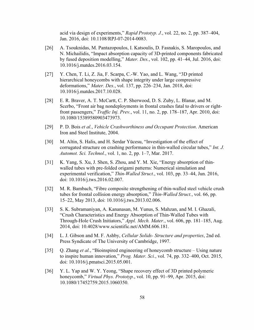
APPENDIX A. CONDITION GRAPHS
Figure A1. Specimen #1 Ambient Conditions
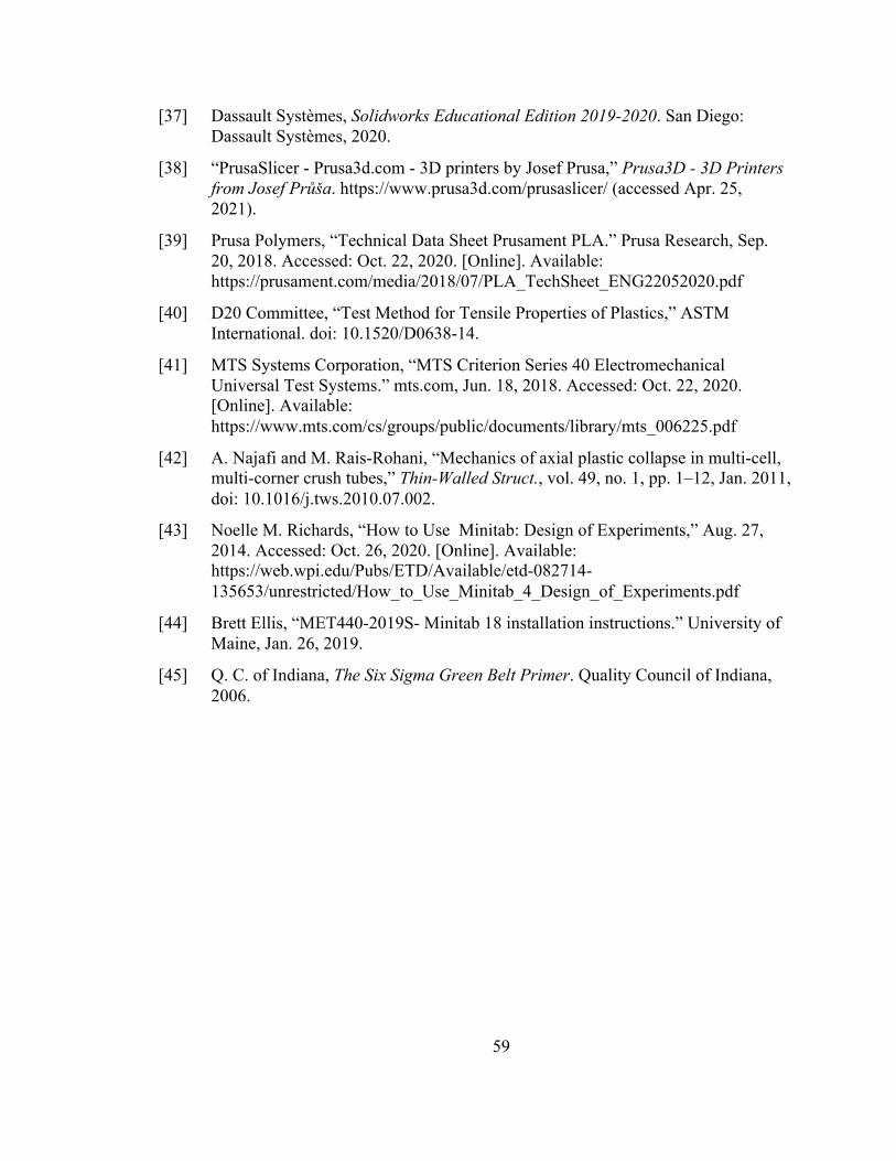
Figure A2. Specimen #2 Ambient Conditions
62
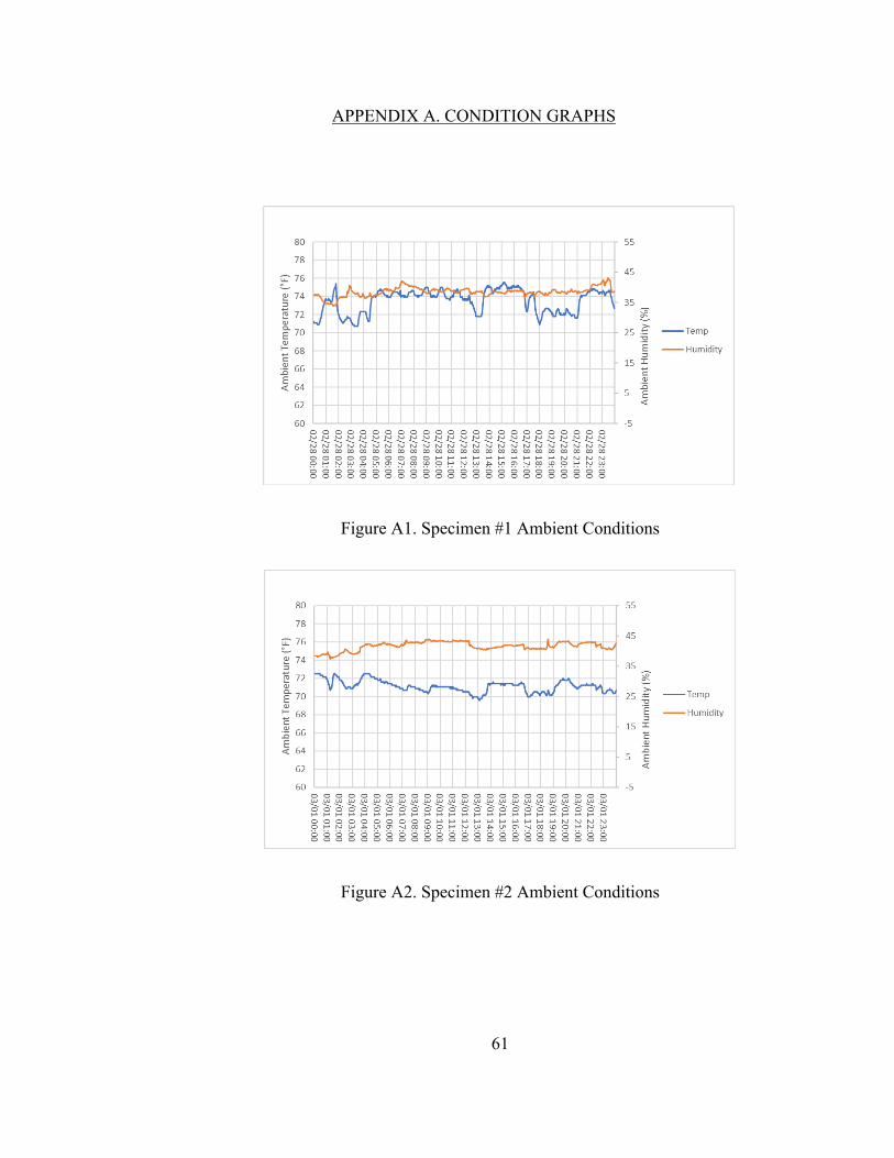
Figure A3. Specimen #3 Ambient Conditions
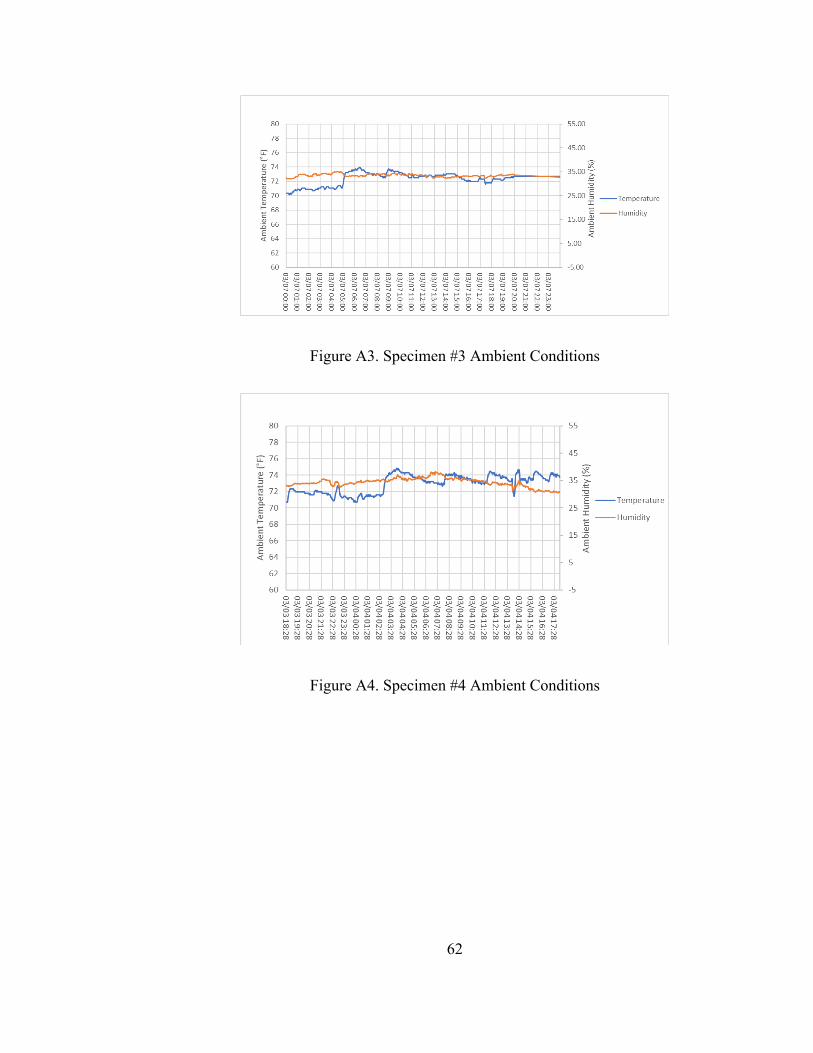
Figure A4. Specimen #4 Ambient Conditions
63
Figure A5. Specimen #5 Ambient Conditions
Figure A6. Specimen #6 Ambient Conditions

64
Figure A7. Specimen #7 Ambient Conditions
Figure A8. Specimen #8 Ambient Conditions
65
Figure A9. Specimen #9 Ambient Conditions
Figure A10. Specimen #10 Ambient Conditions

66
Figure A11. Specimen #11 Ambient Conditions
Figure A12. Specimen #12 Ambient Conditions
67
Figure A13. Specimen #13 Ambient Conditions
Figure A14. Specimen #14 Ambient Conditions
68
Figure A15. Specimen #15 Ambient Conditions
Figure A16. Specimen #16 Ambient Conditions
69
Figure A17. Specimen #17 Ambient Conditions
Figure A18. Specimen #18 Ambient Conditions
70
Figure A19. Specimen #19 Ambient Conditions
Figure A20. Specimen #20 Ambient Conditions
71
APPENDIX B. PRINTER MONITORING GRAPHS
Figure B1. Specimen 1
Time
Tem
pera
ture
(°C)
Te
mpe
ratu
re (°
C)
Time
72
Figure B2. Specimen 2
Figure B3. Specimen 3.
Figure B4. Specimen 4.
Tem
pera
ture
(°C)
Tem
pera
ture
(°C)
Time
Time
73
Figure B5. Specimen 5
Figure B6. Specimen 6
Tem
pera
ture
(°C)
Te
mpe
ratu
re (°
C)
Time
Time
74
Figure B7. Specimen 7
Figure B8. Specimen 8
Tem
pera
ture
(°C)
Te
mpe
ratu
re (°
C)
Time
Time
75
Figure B9. Specimen 9
Figure B10. Specimen 10
Tem
pera
ture
(°C)
Te
mpe
ratu
re (°
C)
Time
Time
76
Figure B11. Specimen 11
Figure B12. Specimen 12
Tem
pera
ture
(°C)
Te
mpe
ratu
re (°
C)
Time
Time
77
Figure B13. Specimen 13
Figure B14. Specimen 14
Tem
pera
ture
(°C)
Te
mpe
ratu
re (°
C)
Time
Time
78
Figure B15. Specimen 15
Figure B16. Specimen 16
Tem
pera
ture
(°C)
Te
mpe
ratu
re (°
C)
Time
Time
79
Figure B17. Specimen 17
Figure B18. Specimen 18
Tem
pera
ture
(°C)
Te
mpe
ratu
re (°
C)
Time
Time

80
Figure B20. Specimen 20
Tensile Specimens
Tem
pera
ture
(°C)
Te
mpe
ratu
re (°
C)
Time
Time

81
AUTHOR’S BIOGRAPHY
Peter Berube was born in Concord, Massachusetts on July 27, 1998. He was
raised in Andover, Massachusetts and graduated from Andover High School in 2017.
Joining the University of Maine as an undeclared engineer, Peter quickly chose to major
in Mechanical Engineering Technology. Peter serves as the Treasurer of the University of
Maine 3D Printing Club as well as a lab technician helping to run the 3D printing lab. He
is a Presidential Scholar in addition to being named to the University of Maine Deans
List. Peter was the 2020-2021 Barbara A. Ouellette Honors Thesis Fellow as well as the
recipient of the Karl Webster Scholarship.
After Graduation, Peter plans to enter the work force, focusing on a career in
project engineering for infrastructure projects in the United States, and plans on returning
to obtain his master’s degree after gaining field experience.