Embed Size (px)
Citation preview

FAA-RD-77-78
Project ReportATC-76
Effects of RF Power Deviations
on BCAS Link Reliability
W. H. Harman
7 June 1977
Lincoln Laboratory MASSACHUSETTS INSTITUTE OF TECHNOLOGY
LEXINGTON, MASSACHUSETTS
Prepared for the Federal Aviation Administration, Washington, D.C. 20591
This document is available to the public through
the National Technical Information Service, Springfield, VA 22161

This document is disseminated under the sponsorship of the Department of Transportation in the interest of information exchange. The United States Government assumes no liability for its contents or use thereof.


Table of Contents
1. INTRODUCTION
2. APPROACH
3. SHRY OF RESULTS
4. DISCUSSION OF RESULTS
5. DERIVATION OF RESULTS
5.1 Characterization of Aircraft Antenna Gain
5.2 Statistical Analysis of Combined Effects
5.3 BCAS Range Requirements
w1
3
4
8
12
12
19
2J
111

1. INTRODUCTION
In the design of BCAS there is some freedom in the choice of specifications
for BCAS transmitter power and receiver MTL (Minimum Triggering Level). Trans-
mitter power should be high enough to provide adequate link reliability and
low enough to prevent interference problems. The question of providing
adequate link reliability is addressed in this study.
A natural or baseline specification worth considering is simply the
assignment of the standard DABS transponder parameters to BCAS namely:
I500 watts nominalBCAS transmitter power (1030 M.) =
(I3 dB tolerance
{
-77 dBm nominalBCAS receiver MTL (1090 ~z) ‘,
~3 dB tolerance
where the levels are referred to the RF port(s) of the BCAS unit. Based on
this assignment, a link power calculation under nominal conditions and at
an air-to-air range of 10 nmi would appear as in Table I. The “nominal margin”
(twO way) aS defined in the table expresses the amount by which receiver power
levels exceed receiver MTL levels in both links. Nom~.nalmargin varies as
a function of range, and also would change if the nominal values in the trans-
mitterfreceiver specification were changed. Although the nominal margin shown
here is 9.5 dB, the actual margin at this range in any particular air-to-air”
encounter may be greater or less due to deviations in any or all the items in

TABLE I
Air-to-Air Link Power Calculation Under Nominal
Conditions and at a Range of 10 nmi.
INTERROGATION REPLYITEM UNITS LINK (1030 ~Z) LINK (109O MHz)
1. transmitter power dBm 57 57
2. transmitter cabling loss dB 3 3
3. transmitter mismatch 10ss dB o 0
4. transmitter antenna gain dB o 0
5. free space path loss dB llB llB.5
6. receiving atltenna gain dB o 0
7. receiving mismatch loss dB o 0
B. receiving cabling loss dB 3 3
9. received power dB,n -67 -67.5
10. MTL dBm -77 -77
11. nominal margin (one way) dB 10 9.5
12. nominal margin (two way) dB 9.5
Notes:i
Items 3 and 7, mismatch losses, refer to the differences, if any,that result when cables are attached to the antennas as comparedwith connections to perfectly matched loads. The nominal value
is arbitrarily taken to be O dB.
Items 4 and 6 -- the nominal value of aircraft antenna gainisarbitrarily taken to be O dB.
Item 5, free space path loss = 20 log(4nR/k) where R = range andA = wavelength.
Item 9, received power equals the sum of items 1, 4, and 6 minusthe sum of items 2, 3, 5, 7, and 8.
Item 10, MTL, denotes Minimum Triggering Level.
Item 11, nominal margin (one way) equals item 9 minus item 10.The small difference originates in free space path loss whichis slightly different at the two frequencies.
Item 12, nominal margin (two way) is the lesser of the two values
in item 11.
2
-----------

the table -- except for free-space path lose wb.ich is entirely predictable.
Thus, for reliable link operation at a given range, it is necessary that a
sufficiently large value of nominal margin be provided by the system design.
It seems reasonable to provide at least enough to offset the sum of the adverse
tolerances for transmitter and receiver, which in this case are 3 dB for trans-
mitter and 3.dB for receiver, totalling 6 dB. Yet a nominal margin of 6 dB may
not be adeqtlfitein view of cabling effects, mismatch effects, and especially
antenna gain effects. This”study approaches the problem of choosing an..adequate
amount of nominal margin from .a statistical point of view.
2. APPROACH
In BCAS; very high link reliability at long ranges improbably not necessary.
Unlike DAESwhich requires very high link reliabitley for all targets under
surveillance (for purposes of deliverin~ IPC comands) , BCAS..probably can
function properly even if””thelink is somewha”t”””intemittant..for some of the
longer range targeta in track. Mat is critical in BCAS .is that for any
aperOa~hing target, detect iOn and threat evaluation be successfully carried
out in time to display appropriate warnings and comands to the pilot . Thus ,
there is a strict requirement on a sort of cumulative link reliability and
no direct requirement for instantaneous link reliability.
Straight flight situations and turning flight situations each present
characteristic problems. In turning flight, aircraft banking tends to increase
the liklihood of deep antenna fades; however, since geometries are continually
changing, these fades are not long lived. In straight flight situations, fades

are more constant, and as a result fades can persist for longer times. Because
BCAS link reliability is to be judged by a cumulative probability, straight
flight may well constitute the more severe test on which the link design shOuld
be based.
When two constant velocity aircraft are on a collision course, the bearing
angle at which each aircraft sees the other is constant. As a result, any
antenna fades which by chance have occurred will persist for the duration of
the encounter up until the point of an escape maneuver. Flight irregularities
due to wind turbulence or any other source would improve the situation, but
for link design purposes, the constant-bearing-angle encounter seems to be a
worst case which can occur atldshould be allowed for.
An analysis has been carried out to indicate the relationship between
nominal margin and BCAS link reliability in this constant b“earing angle worst
case and in an environment free of interference. The approach taken is to
adopt statistical descriptions for each of the deviations in the link calcula-
tion and to combine these ao as to calculate the probability of having adequate
received power for each possible value of nominal margin.
3. SMRY OF RESULTS
Tbe results of this analysis are summarized in Figs. 1 and 2. Figure 1
gives the computed relationship between nominal margin and link reliability,
show for various degrees of antenna diversity. To interpret “link reliability”
plotted vertically in Fig. 1, imagine a population of diversity-equipped air-
craft illwhich the following properties vary from aircraft to aircraft :
4

Fig. 1.and BCAS
/
/
IvE RSITY TO DIVERSITY
DIVERSIT YTO SINGLE ANTENNA
SINGLE ANTE NNA TO SINGLE
/
I I
10 20
NOMINAL MARGIN (dB)
Computed relationship between nominal marginlink reliability. -
5

-
-—....———
~TC-76(2)T
NOTES:
(01
(b)
(c)
99 ?’@ / 1/ /
90 y
DIVERSITY-BOTH AIC
01 1 1 I 1 I
: 90—
/I
, 1 1. or I
REFERS TO THE DABSMODE OF BCAS
IN THE ABSENCE OFINTERFERENCE
TRANSMITTER/RECEIVER 90
PoWER LEVELSREFERRED TO THE BCASUNIT
o L I I 1 1 I50 55 60‘i OMINAL BCAS-TRANSMITTER POWER (dEm)
t 1 , , 1 1 , 1-70 -75 -00
NOMINAL BCAS RECEIVER POWER (dEm)
Fig. 2. BCAS link reliability vs transmitter/receiver specifications.
/
6 I
J..—. -—...
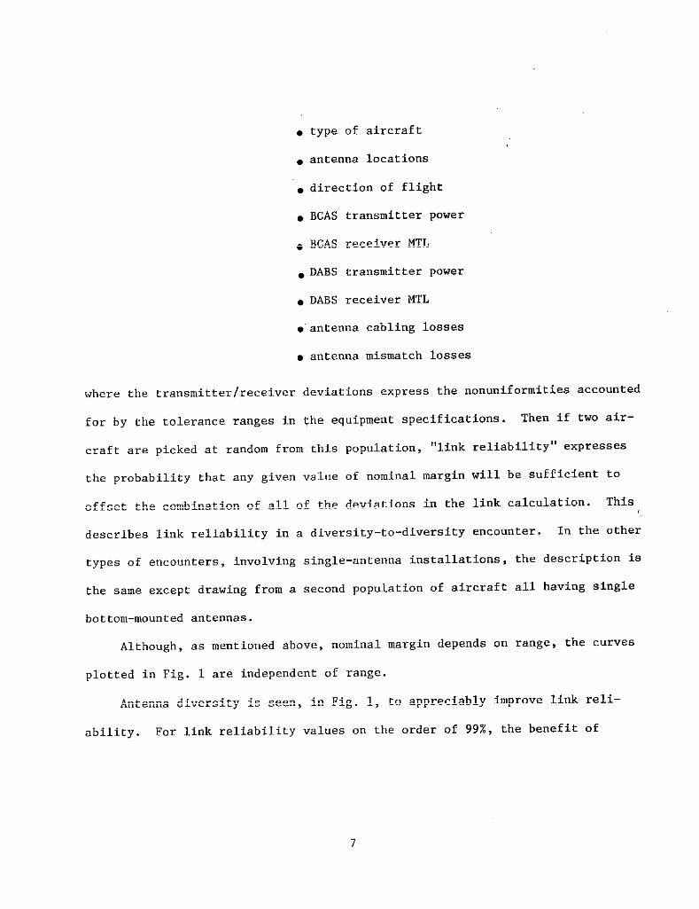
. type of aircraft
. antenna locations
. direction of flight
. BCAS transmitter power
. BCAS receiver MTL
. DABS transmitter power
. DABS receiver MTL
● antenna cabling losses
● antenna mismatch losses
where the transmitter freceiver deviations express the nonuniformities accounted
for by the tolerance ranges in the equipment specifications. Then if twO air-
craft are picked at random from this population, “link reliability” exeresses
the probability that any given value of nnminal margin will be sufficient to
offset the combination of all of the deviations in the link calculation. This
describes link reliability in a diversity-to-diversity encounter. In the other
types of encounters, involving single-antenna installations, the description is
the same except drawing from a second population of aircraft all having single
bottom-mounted antennas.
Although, as mentioned above, nominal margin depends on range, the curves
plotted in Fig. 1 are independent of range.
Antenna diversity is seen, in Fig. 1, to appreciably improve link reli-
ability. For link reliability values on the order of 99%, the benefit of
7
—.4

adding diversity to one aircraft is about equivalent to a 3 dB change in the
transmit ter~receiver specifications, and the benefit of adding diversity to
the other aircraft is another 3 dB. The mechanism causing this diversity bene-
fit in straight flight is diacuased in Section
~len the data of Fig. 1 are cOmbined with
DABS mode of BCAS, the results are as shorn in
5.1.
the range requirements of the
Fig. 2. Here, link reliability
is plotted as a function of the BCAS transmitter/receiver nominal specifica-
tion (varying transmitter and receiver by equal amounts ao as to maintain
balance in the two links). BCAS range requirements depend on closing speed,
and for this reason results are given separately for different values of closing
speed. The results show that, for example, in an encounter with 1200 knot
closing speed, link reliability (in an interference-free environment) is 95%
if both aircraft are diversity equipped,
equipped, and 82% if neither aircraft is
4. DISCUSSION OF RESULTS
ag% if one aircraft
diversity equipped.
is diversity
Before judging the adequacy of transmitter/receiver specifications from
these results, a review of certain inputs t,othe calculation would be appro-
priate. Fig. 3 sumarizes the distributions of transmitter powers, receiver
MTL’a, and antenna cabling and mismatch losses adopted for purposes of this
calculation. These are seen to be idealized rectangular distributions. For
example, BCAS transmitter power is characterized aa being uniformly distri-
buted over the ~3 dB tolerance range. In reality it may be expected that
the distribution would depart from the assumed rectangle possibly having a
concentration near the center part of the tOlerance range, and a mOre gradual
a

~Tc-76(3)~—— —.[ 1
NOMINAL -NOMINAL;/!
, vl///uYA h , I52 54 56 58 60 62 0 2 4 6 8 ;0
1030 T RAN~dMBl:ER” POWER. CABLING LOSS, BCAS AIRCRAFT(dB)
4 1/<NOMINAL &NO.MIN~L..
1
> v//[hY///hl I 8 I:mL1//A “1 t i+ 52 54 56” 58 ::60 62 0 2 4 6 8;.”
zz 1090 TRANSMITTER POWER CABLING LOSS, DABS AIRCRAFTwn
(dBm) (dB)
! , I I . . 1
g 1030 RECEIVER .MTL. ANTENNA MISMATCHLOSS,
>~~
&NOMINAL
m< 1 , v/J//m. ““l Im -82 -80 -70....-76 .-74.. -72
Lo 246810
BCASn (dBm) Aircraft.
!
14 QMINALI
, I 1 “c-B2 -80 -70 -76 -74 -72 024681O
1090 RE(~~:)ER MTL ANTENNA MISMATCH LOSS, DABSAIRCRAFT (dB)
Fig. 3. Probability distributions adopted in this study.
9
-—. m.

fall-off at each end, with some fraction of the population being out of
tolerance above and below. The precise shapes of these distributions would
be difficult to predict. However, as will be discussed in Section 5.2, due
to a central-limit-theorem phenomenon the results of this analysis depend
primarily on means and variances, being otherwise quite insensitive to shapee
of distributions. mile these rectangular distributions are not altogether
realistic, their means and variances appear to be reasonable characterization
(assuming most units are built within the tolerances) , and on this basis the
results given in Figs. 1 and 2 may be accepted as valid.
On the other hand, an assumption that most DABS transponders will
comply with the power and MTL tolerances cannot be taken for granted (as was
demonstrated in the Colby/Crocker ATCRBS transponder test prOgram*). There
are a number of reasons why close agreement ia not aasured between airborne
transponders and the National Standard. Yet, recognizing the possibility
for widespread out-of-tolerance performance brings up the question of whether
or not BCAS should be designed to compensate for such performance. It is our
present opinion that it would not be reasonable to oversize the BCAS trans-
mitter and receiver to bear this burden.
Concerni,~g the concept of link margin, it might be advisable to allocate
a portion of the margin as a “safety factOr” for offsetting possible unexpected
conditions such as departures from the adopted statistical characterizations
I
*Ref. , G.V. Colby and E.A. Crocker, “Final Report, Transponder Test prOgram”,
M.I.T. Lincoln Laboratory, FAA-RD-72-30, 12 April 1972, P. 40-43. For examPle,among general aviation transponders , approximately 40% were out of tOlerancein MTL.

in Fig. 3, and possible changes in the BCAS threat 10gic which wOuld affect
range requirements. In generating Fig. 2, no safety factor waa included,
where instead all of the margin was used to offset effects that are tO be
expe,cted. Additional margin for the unexpected could be provided by simply
adding the appropriate amount
MTL values plotted in Fig. 2.
allowance, althOugh this is a
information becomes available
to the nominal transmitter power and receiver
Our present design does not include such an
preliminary position which could change as new
With these points in mind, the performance shown in Fig. 2 may be judged.
Assuming use of diversity by all BCAS units and by most of the intruders
encountered above 10,000 ft. altitude (where high speed encounters are
possible) , the link performance with the “natural design” values of transmitter
power and receiver MTL appears to be acceptable in the absence of interference.
In a 1200 knot encounter, link reliability is moderately high, and improves
greatly under slower speed conditions.
The conclusions from this work, and
yet to be factored-in,may be sumarized
the relationships with other work
as follows. An appropriate trans-
mitter/receiver specification for the DABS mode of BCAS, providing adequate
link reliability in the absence of interference, iS the “natural design”
(500 watts/-77 dBm) . This design includes sufficient margin for a number of
possible deviations in the air-to-air link, yet it does not include an
additional safety factor for the unexpected. Considerations yet to be in-
cluded are: (1) interference and multipath, (2) the ATCRBS mode of BCAS whose
power requirements may affeet the design of the DABS mode, and
measurements which data when available will either validate or
need for changes in the analytical considerations given here.
(3) link power
indicate the

5. DERIVATION OF RESULTS
5.1 Characterization of Aircraft Antenna Gain
One source of data for aasessing the variability of aircraft antenna
gain is the model measurement program that was carried out by LincOln Labora-
tory and Boeing in 1973-4 (Ref., G .J. Schlieckert, “An Analysis of Aircraft
L-Band Beacon Antenna Patterns”, M.I .T. Lincoln Laboratory, FM-RD-74-144 v
15 January 1975) . An example of these data is shorn in Fig. 4. The plot
includes three cuts from the aircraft antenna pattern of a Gruman Gulfstream,
for o,>eof two bottom antenna positions that were tested. In this example,
an adverse gain variation occurs in the forward direction, in the amount of
about -5 dB. To help in understanding the frequency of occurrence of such
conditions, the data base from the model measurements has been processed in
several ways, one of which leads to the plOts in Fig. 5. In this format, the
data give the cumulative probability distribution of antenna gain values fOr
a population of aircraft orientations. Each curve gives the result for a
single aircraft type and antenna mounting location. The fact that the dif-
ferent curves do not coincide reflects the differences between different
aircraft types and antenna locations. Evidently these differences are large
enough to show UP as statistically significant. The four separate plots in
Fig. 5 correspond to the four combinations of level vs turning flight and
antenna diversity vs a single bottom antenna, where the diversity cases
consist of one bottom antenna together with one top antenna. Level and
turning flight are defined in terns of the following orientation statistics:
12

NOSE90 0
270
“
$z“
E90 90
leoBOTTOM
o
; 90 90z
1 0
180BOTTOM
Fig. 4. Aircraft antenna antenna patterns, from model measurements
(Grwman Gulfstream; bottom mounted, rear antenna, flaps up,wheels up) .

1LEVEL FLIGHT
/
A
0! ——-—-—--–- --- 4
/1111
,
0,
00,
0.0,1
-30 -20 -,0 . ,,
!
0.,
0.01
0,.0,
-,0 -20 -,0 , ,0 -30 -,0 -,0 0 ,0
“,RCRA, T AN,,,,, ,.!, - W,,”OUT 0,”[,,,7”, ,0 ,,,,,.,, ANTENNA GAIN - WITH oIv ERSIIY, DB
Fig. 5. ktenna gain distributions superimposed.
14

“level flight”:
“turning flight”:
azimuth = uniformly distributed over 360°
bank angle = uniformly distributed over -3° to +3°
azimuth = unifomly distributed over 360°
bank angle =
Diversity is expected to offer
when aircraft banking will at times
unifomly distributed over -30° to +30°
its primary advantage in turning situations
shield a single antenna from view, and
this advantage is quite evident in Fig. 5. However, it may seem surprising
at first to see in Fig. 5 th8t diversity offers an appreciable advantage in
level flight situations as well. This advantage results largely from the
horizon-cutoff variability of aircraft antenna patterns -- a phenomenon that
is illustrated in Fig. 6. Here the elevation angle cuts of the Gruman
Gulfstream patterns in Fig. 4 are plotted together and compared with the
pattern of an ideal dipole on a perfect plane. The following properties
are apparent in this plot: (1) Below the horizon and excluding the region
within about 10° of the horizon, the measured’ antenna patterns are moderately
well approximated by the ideal curve. Thus, for example, gains of about +4 dB ,
are typical at about 20° below horizontal. (2) whereas the ideal curve makes
a large and abrupt jump at the horizon, the measured curves have a gradual
horizon cutoff which usually begins below the horizon. (3) The cutoff is
more abrupt in the fore and aft cuts, in which directions the ground plane
is more extensive. (4) This horizon cutoff may be moved up or dom in eleva-
tion angle according to where tbe antenna is mounted. (5) As a result of this
up-Or-dO~ variability and as a result of the steepness of tbe curves around
the horizon, gain values at the horizon have a large spread.
15

10 I
IDEAL DIPOLE/GROUND
ELEVATION ANGLE, c (degl
Fig. 6. Differences in horizon cutoff characteristicsof aircraft antenna patterns.
16

These properties seem to be generally true among all of the aircraft
anterlnapatterns in the data base. The advantage which diversity offers in
level flight results simply from the availability Of twO patterns instead Of
one, which are somewhat
direction.
The data in Fig. S
unlikely to both have low-gain values in a given
have been further reduced by computing probabilities
of antenna gain values for a condition in which the aircraft type and antenna
location are selected at random, with the separate curves in Fig. 5 being
equally likely. The results are shorn in Fig. 7 for level flight, with and
without diversity*. It may be seen here that, for example, there is a 10%
chance of having antenna gain be less than -3 dB for a single antenna instal-
lation, whereas for a diversity installation, the liklihood is abOut 1%.
*If it is true that the diversity benefit in level flight results primarily
from having two independent chances instead Of One, then the twO curves in ‘
Fig. 7 should be related, approximately, by a square law. That is, if pi(G)
and P2 (G) denote the cumulative probability distributions for single-antenna
installations and diversity installations respectively, then it should be
approximately true that
P2(G) = [PI(G)]*, for all G.
The data i“ Fig. 7 can be seen to agree
serves as a reasonableness check of the
with
data
this simple relationship, which
reduction process and of the
conceptual understanding of the diversity benefit.
17
-.--.--..>, s.-..c.-

IATC-76(7) I
995
99
98 F
2
1
0,5 k
DIVER SITY—
30TTOMNA
7
10
AIRCRAFT ANTENNA GAIN (dB)
Fig. 7. Aircraft antenna smary statistics,
18

5.2 Statistical Analysis of Combined Effects
The aircraft antenna characterization in Fig. 7 has been combined with
other effects in the air-to-air link as follows. Define PD (power deviation)
to be
PD = margin (dB) - nominal margin (dB)
where nominal margin is computed as in Table 1, item 12, and where margin ‘a
computed in the same way except under actual conditions rather than nominal
conditions. We proceed to calculate the probability distribution of PD.
The total air-to-air power deviation, PD, is a combination of individual
power deviations of separate effects. The relationships may be expressed
mathematically as follows (based on the form of the link calculation in
Table I)
PD = lesser of (AI + 0.5) and (AR)
where AI and AR are respectively the interrogation link and reply link
deviations, given by
AI = A1O - All - A12 + A13 + A14 - A15 - A16 - A17
AR = A20 - A21 - A22 + A23 + A24 - A25 - A26 - A27
and where A1O, All, etc. , express the deviations of individual terms. These
are defined as follows:
19

tr.
tr.
tr.
tr.
rec.
INTERROGATION REPLY
power (dBm) 57 + A1O 57 + A20
cabling loss (dB) 3 + All 3 + A21
mismatch loss (dB) A12 A22
antenna gain (dB) A13 A23
ant. gain (dB) A14 A24
rec. mismatch loss (dB) A15 A25
rec. cabling loss (dB) 3 + A16 3 + A26
MTL (dBm) -77 + A17 -77 + A27
Each of these is modeled as a random variable with a prespecified probability
distribution, and the resulting probability distribution of
Certain pairs of these variables are related. For example,
refer to the same antenna, only differing in frequency. To
conditions, the following relationships are adopted.
A13 = A24
A14 = A23
All = A26
A16 = A21
PD is calculated.
A13 and A24 both
account for these
Otherwise the variables are taken to be statistically independent. The
antenna gain terms are modeled by the data in Fig. 7 (applicable to level
flight encounters). Deviations in transmitter power and receiver MTL values
are modeled as unifomly distributed over the 33 dB tolerance ranges.

—
A1O
A17
1
= independent, unifomly distributed over (,-3,3)
A20
A27
Cabling losses are modeled as being unifomly distributed over O to 6 dB.
That is
All
!=
independent, uniformly distributed over (-3, 3)
A16
Mismatch losses are modeled as being uniformly distributed over O to 1 dB.
A12 \
A15
/= independent, unifomly distributed over (O, 1)
A22
IA25 ‘
The results were obtained by a computerized Monte Carlo simulation, using
20,000 trials, which is sufficient for stable and accurate results with
probabilities as small as 0.5%, and as large aS gg.5%.
Tbe results for the case in which one aircraft is diversity equipped
and the other is not are shorn in Fig. 8. This plot shows the original
antenna data and some of the intermediate results as well.
It is interesting to observe how the combination of a number of effects
cauaes PD in dB to be approximately a Gausaian random variable. Such “central-
limit-theorem” behavior is generally expected whenever a number of statistically
independent terms are added. This phenomenon is made evident in Fig. 8 which iS
21

~ATG-76(8)i
ROUND-TRIP LINK, PD
,ENNA ~A,N-~,N~~E
I ANTENNA, A14 IENNA GAINS-BOTH
AIRCRAFT, A13 + A14
r{
/:’
2II ‘
II ,’II
f’:+’ ,1
// 1’Ii ,I
\II I
II,1
—
11’
4’I
ANTENNA GAiN-DIVERSITY, All
-lo 0 10
AIR-TO-AIR POWER DEVIATION (dB)
Fig. 8. Power deviation results - BCAS with diversity, intruder without.
22

plotted on Gaussian probability paper (on which any Gaussian distribution
aPPears as a straight line) . The individual antenna gain terms, A13 and A14,
appear ss curved functions and are clearly non-Gsussian. However, when added,
the result (A13 and A14) is seen to be more nearly Gaussian, and when all of
the terms in the interrogation link are combined, the result is accurately
Gaussian over a broad range. It may be concluded from this observation that
the rssults of this analysis have a considerable tolerance to possible
inaccuracies in the original assumptions. The PD results depend almost
entirely on the means and vafiances of the individual terms, being otherwise
independent of the shapes of their probability distributions.
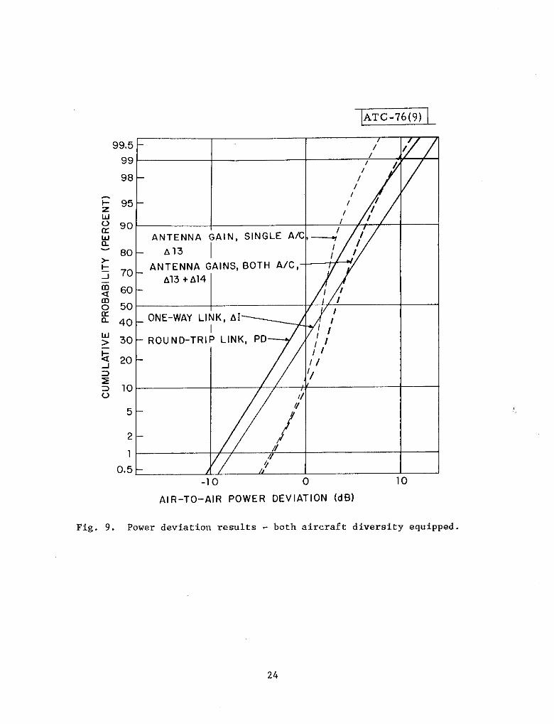
Results were also generated for the case in which both aircraft are
diversity equipped and a case in which neither is diversity equipped. These
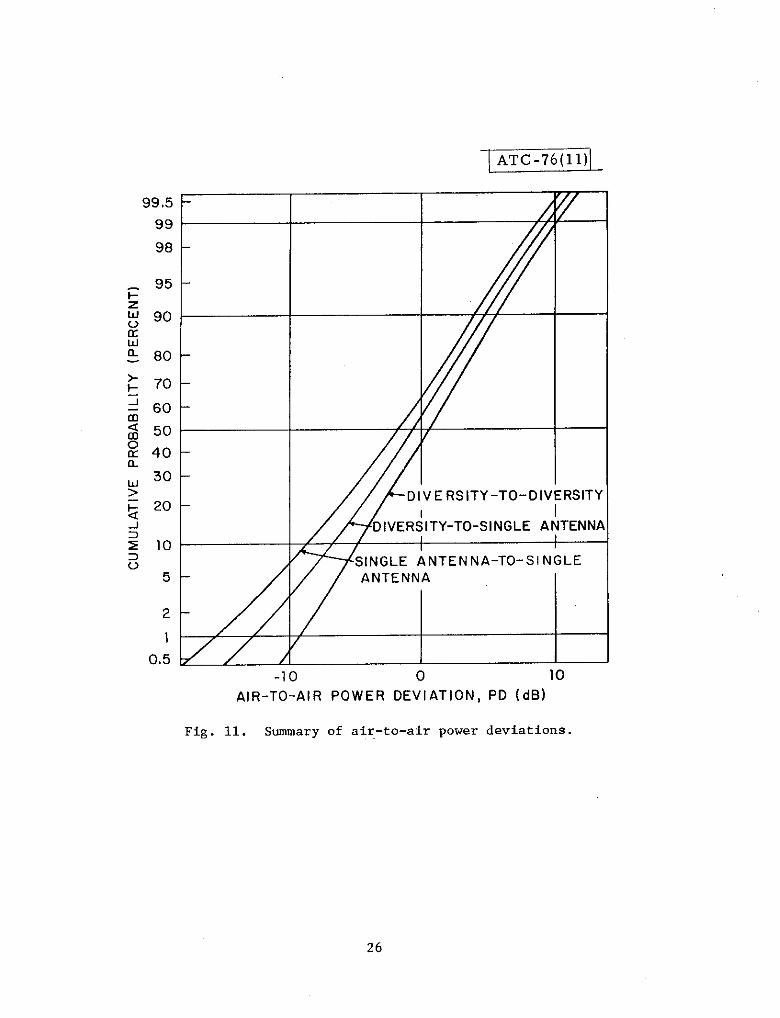
results are given in Figs. 9 and 10. The three cases are summarized in Fig. 11.
The results shorn in Fig. 1 above are exactly the same as in Fig. 11 except
with the axes inverted. That ia, for each value of Nominal Margin (~)
in Fig. 1, Link Reliability (LR) is
LR = prob. (margin ~ O)
which is equivalent to
LR= prob. (PD~-~) = 1 -prob. (PD~-~)
I
Thus LR is the complementary probability (1 minus the probability) that PD
is less than - NN) .
23
98
t
90rANTENNA
80 A13
70ANTENNA ~
A13 +A1460
30t ROUND-TRI
20
10
L5
t2
1
0,5 k
/
/1I
I
f/
IIN, SINGLE AK ,-1
INS, BOTH A/C,
(, AI/
LINK, PD
-10
AIR-TO–AIR POWER
Fig. 9. Power deviation results -
0
OEVIATION (dB)
both aircraft diversity equipped.
24

99,5
99
98
w
2
1
ot5
I ANTENNA GAIN, SINGLE A/C;
IA13 I
ANTENNA GAINS, BOTH A/C,A13+A141
L I ,
/I
– ONE-WAY LINK, AI/
I_ ROUND-TRIP LINK,PD
y//
////
////
/ ,//
/ //
/–-10
,/“ /’
P///
II/’ /
1’ I
A,
‘1I
I
‘/II
z
AIR-TO-AIR POWER DEVIATION (dB)
Fig. 10. Power deviation results - neither aircraft diversity
—
equipped.
25
9985
99
98
2
1
085-1
DIVE RSITY-TO-Dl\
DIVER; ITY-TO-SINGLE A
SINGLE ANTENNA-TO-SINGLE
RSIT\
rENN,
I I
o
AIR-TO-AIR POWER DEVIATION,
Fig. 11. Smary of air-to-air power
26
10
PD (dB)
deviations.

5.3 BCAS Range Requirements
In using these results, it is necessary to specify the maximum range
at which the air-to-air link will be required to operate. The range require-
ments depend on closing speed as illustrated in
the horizontal threat boundary according to the
by a slope of 30 sec. and an offset of 1 nmi) .
velocity encounter would proceed to the left o<
Fig. 12. This plot shows
current BCAS design (described
In such a plot, a constant
a horizontal line, as in
the example plotted. Assuming that, in the DABS mode; up to an additional
10 sec. will be required between the time that the link power becomes
adequate and the time that the threat boundary is penetrated (at which point
a command
nmi for a
This
should be
is to be issued) , it follows that the range requirement is 14.3I
1200 knot encounter. For other closing speeds
Range requirement = 1 nmi + 13.3 nmi (closing speed
1200 kt. )
result is applicable only in the DABS mode, in which case 10 sec.
sufficient to accomplish track acquisition. In the ATCRBS mode, ,
the amount of time required for acquisition strongly depends on surveillance
processing design. In the present baseline design, a time period of about
35 sec. is required. A large performance penalty may result from this long
acquisition time.
The DABS mode range requirements may readily be combined with the power
variation data in Fig. 1. For example, in the 1200 knot encounter for which
the range requirement is 14.3 nmi, the nominal margin at the point of maximum
range is 6.4 dB. According to Fig. 1, the probability of adequate power at
27

\ATC-76(12)]
--
//
.
-+---
-----
PROJECTED COLLISION &
B I ! I I 1
0 5 10 15 20
RANGE (nmi)
Fig. 12. Illustration of BCAS range requirements.
28

that point is 9.5%for a diversity-to-diversity encounter. Calculations of
this sort have been carried out for various closing speeds, for various
levels of diversity, and also for changes in the transmitter and receiver
specifications, producing the results plotted in Fig. 2.