Eur. Phys. J. C (2015) 75:434 DOI 10.1140/epjc/s10052-015-3654-8

Regular Article - Theoretical Physics

Effects of sfermion mixing induced by RGE runningin the minimal flavor violating CMSSM

M. E. Gómez1,a, S. Heinemeyer2,b, M. Rehman2,c

1 Department of Applied Physics, University of Huelva, 21071 Huelva, Spain2 Instituto de Física de Cantabria (CSIC-UC), 39005 Santander, Spain

Received: 15 January 2015 / Accepted: 2 September 2015© The Author(s) 2015. This article is published with open access at Springerlink.com

Abstract Within the Constrained Minimal Supersymmet-ric Standard Model (CMSSM) with Minimal Flavor Vio-lation (MFV) for scalar quarks, we study numerically theeffects of intergenerational squark mixing on B-physicsobservables, electroweak precision observables (EWPO),and the Higgs-boson mass predictions. In models with uni-versal soft terms at the GUT scale, squark mixing is generatedthrough the Renormalization Group Equations (RGEs) run-ning from the GUT scale to the electroweak scale due to pres-ence of non-diagonal Yukawa matrices in the RGEs, e.g. dueto the CKM matrix. Our numerical analysis is based on thecode Spheno for the RGE running and full one-loop calcu-lations, supplemented by further higher-order corrections, atthe electroweak scale of the precision observables as includedin the code FeynHiggs. Taking the CMSSM as a concrete“realistic” example, we find that the B-physics observablesas well as the Higgs mass predictions do not receive sizablecorrections. On the other hand, in our numerical analysis weobserve that the EWPO such as theW boson mass can receiverelevant corrections. Such contributions could in principle beused to place new bounds on the CMSSM parameter space.We extend our numerical analysis to the CMSSM extendedwith a mechanism to explain neutrino masses (CMSSM-seesaw I), which induces flavor violation in the scalar leptonsector. The effects of slepton mixing on the analyzed observ-ables are found to be, in general, smaller than those of squarkmixing, but in our numerical analysis reach the level of thecurrent experimental uncertainty for the EWPO.

M. Rehman is a MulitDark Scholar.

a e-mail: mario.gomez@dfa.uhu.esb e-mail: Sven.Heinemeyer@cern.chc e-mail: rehman@ifca.unican.es

1 Introduction

Supersymmetric (SUSY) extensions of the Standard Model(SM) are broadly considered as the most motivated andpromising New Physics (NP) theories beyond the SM. Thesolution of the hierarchy problem, the gauge coupling unifi-cation and the possibility of having a natural cold dark mattercandidate, constitute the most convincing arguments in favorof SUSY.

Within the Minimal Supersymmetric Standard Model(MSSM) [1–3], flavor mixing can occur in both scalar quarkand scalar lepton sector. Here the possible presence of softSUSY-breaking parameters in the squark and slepton sector,which are off-diagonal in flavor space (mass parameters aswell as trilinear couplings) are the most general way to intro-duce flavor mixing within the MSSM. This, however, yieldsmany new sources of flavor and CP-violation, which poten-tially lead to large non-standard effects in flavor processes,in conflict with the experimental bounds.

The SM has been very successfully tested by low-energyflavor observables both from the kaon and the Bd sectors. Inparticular, the two B factories have established that Bd fla-vor and CP-violating processes are well described by the SMup to an accuracy of the ∼10 % level [4]. This immediatelyimplies a tension between the solution of the hierarchy prob-lem, calling for a NP scale at or below the TeV scale, and theexplanation of the flavor physics data, requiring a multi-TeVNP scale, if the new flavor-violating couplings are of genericsize.

An elegant way to simultaneously solve the above prob-lems is provided by the Minimal Flavor Violation (MFV)hypothesis [5–8], where flavor and CP-violation in the quarksector are assumed to be entirely described by the CKMmatrix, even in theories beyond the SM. For example inMSSM, the off-diagonality in the sfermion mass matrixreflects the misalignment (in flavor space) between fermionsand sfermions mass matrices, which cannot be diagonalized

123

434 Page 2 of 26 Eur. Phys. J. C (2015) 75:434

simultaneously. This misalignment can be produced fromvarious origins. For instance, off-diagonal sfermion massmatrix entries can be generated by Renormalization GroupEquations (RGE) running. Going from a high energy scale,where no flavor violation is assumed, down to the elec-troweak (EW) scale, such entries can be generated due to thepresence of non-diagonal Yukawa matrices in the RGEs. Forinstance, in the Constrained Minimal Supersymmetric Stan-dard Model (CMSSM, see [9] and references therein), theRGE effects on non-diagonal sfermion soft SUSY-breakingparameters are affected only by non-diagonal elements on theYukawa couplings and the trilinear terms which are taken asproportional to the Yukawas at the GUT scale. We choosethe following form of the Yukawa matrices (working in theSuper-CKM basis [10]):

YD = diag(yd , ys, yb), YU = V †CKMdiag(yu, yc, yt ). (1)

Hence, all flavor violation in the quark and squark sec-tor is generated by the RGEs and controlled by the CKMmatrix, i.e. the Yukawa couplings have a strong impact on thesize of the induced off-diagonal entries in the squark massmatrices.

The situation is somewhat different in the slepton sec-tor where neutrinos are strictly massless (in the SM and theMSSM). Consequently, there is no slepton mixing, whichwould induce Lepton Flavor Violation (LFV) in the chargedsector, allowing not yet observed processes like li → l jγ(i > j ; l3,2,1 = τ, μ, e) [11]. However, in the neutral sec-tor, we have strong experimental evidence that shows thatthe neutrinos are massive and mix among themselves [12–20]. In order to incorporate this, one needs to go beyondthe MSSM to introduce a mechanism that generates neu-trino masses. The simplest way would be to introduce Diracmasses, leaving, however, the extreme smallness of the neu-trino masses unexplained. To overcome this problem, typ-ically a seesaw mechanism is used to generate neutrinomasses, and the PMNS matrix plays the role of the CKMmatrix in the lepton sector. Extending the MFV hypothesis forleptons [21] we can assume that the flavor mixing in the lep-ton and slepton sector is induced and controlled by the seesawmechanism.

Consequently, in this paper we will numerically inves-tigate two “realistic” models (more detailed definitions aregiven in the next section):

(i) the CMSSM, where only flavor violation in the squarksector is present;

(ii) the CMSSM augmented by the seesaw type I mechanism[22–28], called “CMSSM-seesaw I” below.

In many analyses of the CMSSM, or extensions such asthe NUHM1 or NUHM2 (see [9] and references therein), the

hypothesis of MFV has been used, and it has been assumedthat the contributions coming from MFV are negligible forother observables as well; see, e.g., [29–32]. In this paperwe will perform a numerical analysis to see whether thisassumption is justified, and whether including these MFVeffects could in principle lead to additional constraints onthe CMSSM parameter space. However, we do not attemptto find analytical solutions to analyze this, as they becomeextremely involved in the presence of intergenerational mix-ing in SUSY models. In this respect we numerically evaluatein the CMSSM and in the CMSSM-seesaw I the followingset of observables: B physics observables (BPO), in partic-ular BR(B → Xsγ ), BR(Bs → μ+μ−) and �MBs , elec-troweak precision observables (EWPO), in particular MW

and the effective weak leptonic mixing angle, sin2 θeff , aswell as the masses of the neutral and charged Higgs bosonsin the MSSM.

In order to perform our calculations, we use the codeSPheno [33,34] to generate the CMSSM (containing alsothe type I seesaw) particle spectrum by running RGE from theGUT down to the EW scale. The effects of the CKM matrixin the RGE running on the mixing in the scalar fermion sectorthus fully relies on the SPheno implementation. The parti-cle spectrum was then handed over in the form of an SLHAfile [10,35] to FeynHiggs [36–41] to calculate EWPO andHiggs-boson masses. The B physics observables were cal-culated by the BPHYSICS subroutine included in the SuFlacode [42,43] (see also [44–46] for the improved version usedhere).

Our setup provides an evaluation of flavor-violatingeffects in “realistic” MFV models (where flavor violationenters only via RGE running) using state-of-the-art tools,compared to state-of-the-art limits, where the size of theeffects will also be compared to future sensitivities. Effectsthat may appear negligible now might be non-negligible inthe future. Furthermore, in the case of lepton-flavor viola-tion [case (ii) above], we are not aware of any analysis of thistype.

The paper is organized as follows: First we review themain features of the MSSM with sfermion flavor mixing inMFV in Sect. 2. The computational setup is given in Sect.3. The numerical results are presented in Sect. 4, where firstwe discuss the effect of squarks mixing in the CMSSM. In asecond step we analyze the effects of slepton mixing i.e. theCMSSM-seesaw I. Our conclusions can be found in Sect. 5.

2 Model setup

In this section we will first review the CMSSM and the con-cept of MFV. Subsequently, we will discuss the MSSM, itsseesaw extension and parameterization of sfermion mixingat low energy.

123

Eur. Phys. J. C (2015) 75:434 Page 3 of 26 434

2.1 The CMSSM and MFV

The MSSM is the simplest supersymmetric structure we canbuild from the SM particle content. The general setup for thesoft SUSY-breaking parameters is given by [1–3]

− Lsoft = (m2Q)ji q

†iL qL j + (m2

u)ij u

∗Ri u

jR + (m2

d)ij d

∗Ri d

jR

+ (m2L)ji l

†iL lL j + (m2

e)ij e

∗Ri e

jR + m2

1h†1h1

+m22h

†2h2 + (Bμh1h2 + h.c.) +

(Ai jd h1d

∗Ri qL j

+Ai ju h2u

∗Ri qL j + Ai j

l h1e∗Ri lL j + 1

2M1 B

0L B

0L

+1

2M2W

aL W

aL + 1

2M3G

aGa + h.c.

). (2)

Here m2Q

and m2L

are 3 × 3 matrices in family space

(with i, j being the generation indices) for the soft massesof the left-handed squark qL and slepton lL SU (2) dou-blets, respectively. m2

u , m2d, and m2

e contain the soft massesfor right-handed up-type squarks u R , down-type squarksdR , and charged slepton eR SU (2) singlets, respectively.Au , Ad , and Al are the 3 × 3 matrices for the trilin-ear couplings for up-type squarks, down-type squarks, andcharged slepton, respectively; m1 and m2 are the softmasses of the Higgs sector. In the last line M1, M2, andM3 define the bino, wino, and gluino mass terms, respec-tively.

Within the constrained MSSM the soft SUSY-breakingparameters are assumed to be universal at the Grand Unifi-cation scale MGUT ∼ 2 × 1016 GeV,

(m2Q)i j = (m2

U )i j = (m2D)i j = (m2

L)i j = (m2E )i j = m2

0 δi j ,

m2H1

= m2H2

= m20, mg = mW = mB = m1/2,

(AU )i j = A0eiφA (YU )i j , (AD)i j = A0e

iφA (YD)i j ,

(AE )i j = A0eiφA (YE )i j . (3)

There is a common mass for all the scalars,m20, a single gaug-

ino mass, m1/2, and all the trilinear soft-breaking terms aredirectly proportional to the corresponding Yukawa couplingsin the superpotential with a proportionality constant A0eiφA ,containing a potential non-trivial complex phase.

With the use of the Renormalization Group Equations(RGE) of the MSSM, one can obtain the SUSY spectrumat the EW scale. All the SUSY masses and mixings are thengiven as a function of m2

0, m1/2, A0, and tan β = v2/v1,the ratio of the two vacuum expectation values (see below).We require radiative symmetry breaking to fix |μ| and |Bμ|[47,48] with the tree-level Higgs potential.

By definition, this model fulfills the MFV hypothesis,since the only flavor-violating terms stem from the CKMmatrix. The important point is that, even in a model withuniversal soft SUSY-breaking terms at some high energy

scale as the CMSSM, some off-diagonality in the squarkmass matrices appears at the EW scale. Working in thebasis where the squarks are rotated parallel to the quarks,the so-called Super CKM (SCKM) basis, the squark massmatrices are not flavor diagonal at the EW scale. This isdue to the fact that at MGUT there exist two non-trivialflavor structures, namely the two Yukawa matrices for theup and down quarks, which are not simultaneously diago-nalizable. This implies that through RGE evolution someflavor mixing leaks into the sfermion mass matrices. In ageneral SUSY model the presence of new flavor structuresin the soft SUSY-breaking terms would generate large fla-vor mixing in the sfermion mass matrices. However, in theCMSSM, which we are investigating here, the two Yukawamatrices are the only source of flavor change. As alwaysin the SCKM basis, any off-diagonal entry in the sfermionmass matrices at the EW scale will be necessarily propor-tional to a product of Yukawa couplings. The RGEs forthe soft SUSY-breaking terms are sets of linear equations,and, thus, to match the correct chirality of the coupling,Yukawa couplings or trilinear soft terms must enter the RGEin pairs. (The same holds for the CMSSM-seesaw I; seebelow.)

2.2 MSSM and its seesaw extension

One can write the most general SU (3)C × SU (2)L ×U (1)Ygauge invariant and renormalizable superpotential as

WMSSM = Y i je εαβH

α1 Ec

i Lβj + Y i j

d εαβHα1 Dc

i Qβj

+Y i ju εαβH

α2 U

ci Q

βj + μεαβH

α1 Hβ

2 (4)

where Li represents the chiral multiplet of a SU (2)L doubletlepton, Ec

i a SU (2)L singlet charged lepton, H1 and H2 twoHiggs doublets with opposite hypercharge. Similarly Q, U ,and D represent chiral multiplets of quarks of a SU (2)Ldoublet and two singlets with differentU (1)Y charges. Threegenerations of leptons and quarks are assumed and thus thesubscripts i and j run over 1 to 3. The symbol εαβ is ananti-symmetric tensor with ε12 = 1.

In order to provide an explanation for the (small) neu-trino masses, the MSSM can be extended by the type-I see-saw mechanism [22–28]. The superpotential for CMSSM-seesaw I can be written as

W = WMSSM + Y i jν εαβH

α2 Nc

i Lβj + 1

2Mi j

N Nci N

cj , (5)

where WMSSM is given in Eq. (4) and Nci is the additional

superfield that contains the three right-handed neutrinos, νRi ,and their scalar partners, νRi . M

i jN denotes the 3×3 Majorana

mass matrix for heavy right-handed neutrino. The full set ofsoft SUSY-breaking terms is given by

123

434 Page 4 of 26 Eur. Phys. J. C (2015) 75:434

− Lsoft,SI = −Lsoft + (m2ν )

ij ν

∗Ri ν

jR

+(

1

2Bi j

ν Mi jN ν∗

Ri ν∗Rj + Ai j

ν h2ν∗Ri lL j + h.c.

),

(6)

with Lsoft given by Eq. (2), (m2ν)ij , A

i jν , and Bi j

ν are the newsoft-breaking parameters.

By the seesaw mechanism three of the neutral fieldsacquire heavy masses and decouple at high energy scale thatwe will denote MN ; below this scale the effective theory con-tains the MSSM plus an operator that provides masses to theneutrinos.

W = WMSSM + 1

2(YνLH2)

T M−1N (YνLH2). (7)

This framework naturally explains neutrino oscillationsin agreement with experimental data [12–20]. At the elec-troweak scale an effective Majorana mass matrix for lightneutrinos,

meff = −1

2v2uYν · M−1

N · Y Tν , (8)

arises from Dirac neutrino YukawaYν (which can be assumedof the same order as the charged-lepton and quark Yukawas),and heavy Majorana masses MN . The smallness of theneutrino masses implies that the scale MN is very high,O(1014 GeV).

From Eqs. (5) and (6) we can observe that one canchoose a basis such that the Yukawa coupling matrix, Y i j

l ,

and the mass matrix of the right-handed neutrinos, Mi jN ,

are diagonalized as Y δl and Mδ

R , respectively. In this case

the neutrino Yukawa couplings Y i jν are not generally diag-

onal, giving rise to LFV. Here it is important to note thatthe lepton-flavor conservation is not a consequence of theSM gauge symmetry, even in the absence of the right-handed neutrinos. Consequently, slepton-mass terms can vio-late the lepton-flavor conservation in a manner consistentwith the gauge symmetry. Thus the scale of LFV can beidentified with the EW scale, much lower than the right-handed neutrino scale MN , leading to potentially observablerates.

In the SM augmented by right-handed neutrinos, theflavor-violating processes such as μ → eγ , τ → μγ etc.,whose rates are proportional to inverse powers of Mδ

R , wouldbe highly suppressed with such a large MN scale, and henceare far beyond current experimental bounds. However, inSUSY theories, the neutrino Dirac couplings Yν enter inthe RGEs of the soft SUSY-breaking sneutrino and slep-ton masses, generating LFV. In the basis where the charged-lepton masses Y� is diagonal, the soft slepton-mass matrixacquires corrections that contain off-diagonal contributionsfrom the RGE running from MGUT down to the Majorana

mass scale MN , of the following form (in the leading-logapproximation) [49]:

(m2L)i j ∼ 1

16π2 (6m20 + 2A2

0)(Yν†Yν)i j log

(MGUT

MN

)

(m2e)i j ∼ 0 (9)

(Al)i j ∼ 3

8π2 A0Yl i (Yν†Yν)i j log

(MGUT

MN

)

Consequently, even if the soft scalar masses were univer-sal at the unification scale, quantum corrections between theGUT scale and the seesaw scale MN would modify this struc-ture via renormalization-group running, which generates off-diagonal contributions [50–55] at MN in a basis such that Y�

is diagonal. Below this scale, the off-diagonal contributionsremain almost unchanged.

Therefore the seesaw mechanism induces non-trivial val-ues for slepton δFAB

i j resulting in a prediction for LFV decaysli → l jγ , (i > j) that can be much larger than the non-SUSY case. These rates depend on the structure of Yν at aseesaw scale MN in a basis where Yl and MN are diagonal.By using the approach of [55] a general form of Yν contain-ing all neutrino experimental information can be written as

Yν =√

2

vu

√Mδ

R R√mδ

νU† , (10)

where R is a general orthogonal matrix and mδν denotes the

diagonalized neutrino mass matrix. In this basis the matrixUcan be identified with the UPMNS matrix obtained as

mδν = UTmeffU. (11)

In order to find values for the slepton generation mixingparameters we need a specific form of the product Y †

ν Yν asshown in Eq. (9). The simple consideration of direct hierar-chical neutrinos with a common scale for right-handed neu-trinos provides a representative reference value. In this caseusing Eq. (10) we find

Y †ν Yν = 2

v2uMRUmδ

νU†. (12)

Here MR is the common mass assigned to the νR . In theconditions considered here, LFV effects are independent ofthe matrix R.

For the numerical analysis the values of the Yukawa cou-plings etc. have to be set to yield values in agreement withthe experimental data for neutrino masses and mixings. Inour computation, by considering a normal hierarchy among

the neutrino masses, we fix mν3 ∼√

�m2atm ∼ 0.05 eV and

require mν2/mν3 = 0.17, mν2 ∼ 100 · mν1 consistent withthe measured values of �m2

sol and �m2atm [56]. The matrixU

123

Eur. Phys. J. C (2015) 75:434 Page 5 of 26 434

is identified with UPMNS with the CP-phases set to zero andneutrino mixing angles set to the center of their experimentalvalues.

One can observe that meff remains unchanged by consis-tent changes on the scales of MN and Yν . This is no longercorrect for the off-diagonal entries in the slepton-mass matri-ces (parameterized by slepton δFAB

i j , see the next subsec-tion). These quantities have a quadratic dependence on Yν

and a logarithmic dependence on MN ; see Eq. (9). Thereforelarger values of MN imply larger LFV effects. By settingMN = 1014 GeV, the largest values of Yν are of about 0.29,this implies an important restriction on the parameters spacearising from the BR(μ → eγ ) as will be discussed in Sects.3 and 4. An example of models with almost degenerate νRcan be found in [50]. For our numerical analysis we testedseveral scenarios and we found that the one defined here isthe simplest and also the one with larger LFV prediction.

2.3 Scalar fermion sector with flavor mixing

In this section we give a brief description about how weparameterize flavor mixing at the EW scale. We are usingthe same notation as in [44–46,57,58]. However, while inthis section we give a general description, in our analysisbelow, contrary to our previous analyses [57], this time weconcentrate on the origin of the flavor mixing as discussed inthe previous sections.

The most general hypothesis for flavor mixing assumesa mass matrix that is not diagonal in flavor space, both forsquarks and sleptons. In the squarks sector and charged slep-ton sector we have 6 × 6 mass matrices, based on the corre-sponding six electroweak interaction eigenstates, UL ,R withU = u, c, t for up-type squarks, DL ,R with D = d, s, b fordown-type squarks and L L ,R with L = e, μ, τ for chargedsleptons. For the sneutrinos we have a 3×3 mass matrix, sincewithin the MSSM even with type I seesaw (right-handedneutrinos decouple below their respective mass scale) wehave only three electroweak interaction eigenstates, νL withν = νe, νμ, ντ .

The non-diagonal entries in this 6 × 6 general matrix forsfermions can be described in terms of a set of dimensionlessparameters δFAB

i j (F = Q,U, D, L , E; A, B = L , R; i, j =1, 2, 3, i �= j) where F identifies the sfermion type, L , Rrefer to the “left-” and “right-handed” SUSY partners of thecorresponding fermionic degrees of freedom, and i, j indicesrun over the three generations. (Non-zero values for the δFAB

i jare generated via the processes discussed in the previoussubsections.)

One usually writes the 6 × 6 non-diagonal mass matri-ces, M2

u and M2d, referred to the Super-CKM basis, being

ordered, respectively, as (uL , cL , tL , u R, cR, tR), (dL , sL ,

bL , dR, sR, bR) and M2l

referred to the Super-PMNS basis,

being ordered as (eL , μL , τL , eR, μR, τR), and write themin terms of left- and right-handed blocks M2

q AB , M2l AB

(q = u, d, A, B = L , R), which are non-diagonal 3 × 3matrices,

M2q =

⎛⎝ M2

q LL M2q L R

M2 †q L R M2

q RR

⎞⎠ , q = u, d, (13)

where

M2u LL i j = m2

UL i j+ (m2

ui + (T u3 − Qus

2w)M2

Z cos 2β)δi j ,

M2u RR i j = m2

UR i j+ (m2

ui + Qus2wM

2Z cos 2β)δi j ,

M2u L R i j = 〈H0

2〉Aui j − mui μ cot β δi j , (14)

M2d LL i j

= m2DL i j

+ (m2di + (T d

3 − Qds2w)M2

Z cos 2β)δi j ,

M2d RR i j

= m2DR i j

+ (m2di + Qds

2wM

2Z cos 2β)δi j ,

M2d L R i j

= 〈H01〉Ad

i j − mdiμ tan β δi j ,

and

M2l

=⎛⎝ M2

l LLM2

l L R

M2 †l L R

M2l RR

⎞⎠ , (15)

where

M2l LL i j

= m2L i j

+(m2

li +(

−1

2+ s2

w

)M2

Z cos 2β

)δi j ,

M2l RR i j

= m2E i j

+ (m2li − s2

wM2Z cos 2β)δi j , (16)

M2l L R i j

= 〈H01〉Al

i j − mliμ tan β δi j ,

with, i, j = 1, 2, 3, Qu = 2/3, Qd = −1/3, T u3 = 1/2, and

T d3 = −1/2. The MZ ,W denote the Z and W boson masses,

with s2w = 1 − M2

W /M2Z = 1 − c2

w, and (mu1 ,mu2 ,mu3) =(mu,mc,mt ), (md1,md2 ,md3) = (md ,ms,mb) are thequark masses and (ml1,ml2 ,ml3) = (me,mμ,mτ ) are thelepton masses. μ is the Higgsino mass term and tan β =v2/v1 with v1 = 〈H0

1〉 and v2 = 〈H02〉 being the two vac-

uum expectation values of the corresponding neutral Higgsboson in the Higgs SU (2)L doublets, H1 = (H0

1 H−1 ) and

H2 = (H+2 H0

2).It should be noted that the non-diagonality in flavor comes

exclusively from the soft SUSY-breaking parameters, thatcould be non-vanishing for i �= j , namely: the massesmQ i j and mL i j for the sfermion SU (2) doublets, the masses

m2UL i j

, m2UR i j

, m2DL i j

, m2DR i j

, mE i j for the sfermion SU (2)

singlets and the trilinear couplings, A fi j .

In the sneutrino sector there is, correspondingly, a one-block 3×3 mass matrix, that is referred to the (νeL , νμL , ντ L)

electroweak interaction basis:

123

434 Page 6 of 26 Eur. Phys. J. C (2015) 75:434

M2ν = (M2

ν LL), (17)

where

M2ν LL i j = m2

L i j+

(1

2M2

Z cos 2β

)δi j . (18)

It is important to note that due to SU (2)L gauge invari-ance the same soft masses mQ i j enter in both up-type anddown-type squarks mass matrices similarly mL i j enter inboth the slepton and the sneutrino LL mass matrices. Thesoft SUSY-breaking parameters for the up-type squarks dif-fer from corresponding ones for down-type squarks by a rota-tion with CKM matrix. The same would hold for sleptons i.e.the soft SUSY-breaking parameters of the sneutrinos woulddiffer from the corresponding ones for charged sleptons bya rotation with the PMNS matrix. However, taking the neu-trino masses and oscillations into account in the SM leadsto LFV effects that are extremely small. For instance, inμ → eγ they are of O(10−47) in the case of Dirac neu-trinos with mass around 1 eV and maximal mixing [59–62],and of O(10−40) in the case of Majorana neutrinos [59,62].Consequently we do not expect large effects from the inclu-sion of neutrino mass effects here and neglect a rotation withthe PMNS matrix. The sfermion mass matrices in terms ofthe δFAB

i j are given as

m2UL

=

⎛⎜⎜⎜⎝

m2Q1

δQLL12 mQ1

mQ2δQLL13 mQ1

mQ3

δQLL21 mQ2

mQ1m2

Q2δQLL23 mQ2

mQ3

δQLL31 mQ3

mQ1δQLL32 mQ3

mQ2m2

Q3

⎞⎟⎟⎟⎠,

(19)

m2DL

= V †CKM m2

ULVCKM, (20)

m2UR

=

⎛⎜⎜⎝

m2U1

δURR12 mU1

mU2δURR

13 mU1mU3

δURR21 mU2

mU1m2

U2δURR

23 mU2mU3

δURR31 mU3

mU1δURR

32 mU3mU2

m2U3

⎞⎟⎟⎠,

(21)

m2DR

=

⎛⎜⎜⎝

m2D1

δDRR12 mD1

mD2δDRR

13 mD1mD3

δDRR21 mD2

mD1m2

D2δDRR

23 mD2mD3

δDRR31 mD3

mD1δDRR

32 mD3mD2

m2D3

⎞⎟⎟⎠,

(22)

v2Au =

⎛⎜⎜⎝

mu Au δULR12 mQ1

mU2δULR

13 mQ1mU3

δULR21 mQ2

mU1mcAc δULR

23 mQ2mU3

δULR31 mQ3

mU1δULR

32 mQ3mU2

mt At

⎞⎟⎟⎠,

(23)

v1Ad =

⎛⎜⎜⎝

md Ad δDLR12 mQ1

mD2δDLR

13 mQ1mD3

δDLR21 mQ2

mD1ms As δDLR

23 mQ2mD3

δDLR31 mQ3

mD1δDLR

32 mQ3mD2

mbAb

⎞⎟⎟⎠,

(24)

m2L

=

⎛⎜⎜⎝

m2L1

δLLL12 mL1mL2

δLLL13 mL1mL3

δLLL21 mL2mL1

m2L2

δLLL23 mL2mL3

δLLL31 mL3mL1

δLLL32 mL3mL2

m2L3

⎞⎟⎟⎠ ,

(25)

v1Al =

⎛⎜⎜⎝

meAe δELR12 mL1

mE2δELR

13 mL1mE3

δELR21 mL2

mE1mμAμ δELR

23 mL2mE3

δELR31 mL3

mE1δELR

32 mL3mE2

mτ Aτ

⎞⎟⎟⎠ ,

(26)

m2E

=⎛⎜⎝

m2E1

δERR12 mE1

mE2δERR

13 mE1mE3

δERR21 mE2

mE1m2

E2δERR

23 mE2mE3

δERR31 mE3

mE1δERR

32 mE3mE2

m2E3

⎞⎟⎠ .

(27)

In all this work, for simplicity, we are assuming that allδFABi j parameters are real and, therefore, hermiticity of M2

Q,

M2l, and M2

νimplies δFAB

i j = δFBAji .

The next step is to rotate the squark states from the Super-CKM basis, qL ,R , to the physical basis. If we set the order inthe Super-CKM basis as above, (uL , cL , tL , u R, cR, tR) and(dL , sL , bL , dR, sR, bR), and in the physical basis as u1,...,6

and d1,...,6, respectively, these last rotations are given by two

6 × 6 matrices, Ru and Rd ,

⎛⎜⎜⎜⎜⎜⎜⎜⎜⎝

u1

u2

u3

u4

u5

u6

⎞⎟⎟⎟⎟⎟⎟⎟⎟⎠

= Ru

⎛⎜⎜⎜⎜⎜⎜⎜⎜⎜⎝

uL

cL

tL

u R

cR

tR

⎞⎟⎟⎟⎟⎟⎟⎟⎟⎟⎠

,

⎛⎜⎜⎜⎜⎜⎜⎜⎜⎜⎝

d1

d2

d3

d4

d5

d6

⎞⎟⎟⎟⎟⎟⎟⎟⎟⎟⎠

= Rd

⎛⎜⎜⎜⎜⎜⎜⎜⎜⎜⎝

dL

sL

bL

dR

sR

bR

⎞⎟⎟⎟⎟⎟⎟⎟⎟⎟⎠

, (28)

yielding the diagonal mass-squared matrices for squarks asfollows:

diag{m2u1

,m2u2

,m2u3

,m2u4

,m2u5

,m2u6

} = Ru M2u Ru†, (29)

diag{m2d1

,m2d2

,m2d3

,m2d4

,m2d5

,m2d6

} = Rd M2dRd†. (30)

Similarly we need to rotate the sleptons and sneutrinosfrom the electroweak interaction basis to the physical masseigenstate basis,

123

Eur. Phys. J. C (2015) 75:434 Page 7 of 26 434

⎛⎜⎜⎜⎜⎜⎜⎜⎝

l1l2l3l4l5l6

⎞⎟⎟⎟⎟⎟⎟⎟⎠

= Rl

⎛⎜⎜⎜⎜⎜⎜⎝

eLμL

τLeRμR

τR

⎞⎟⎟⎟⎟⎟⎟⎠

,

⎛⎝ ν1

ν2

ν3

⎞⎠ = Rν

⎛⎝ νeL

νμL

ντ L

⎞⎠ , (31)

with Rl and Rν being the respective 6 × 6 and 3 × 3 uni-tary rotating matrices that yield the diagonal mass-squaredmatrices as follows:

diag{m2l1,m2

l2,m2

l3,m2

l4,m2

l5,m2

l6} = Rl M2

lRl†, (32)

diag{m2ν1

,m2ν2

,m2ν3

} = Rν M2ν Rν†. (33)

3 Computational setup

Here we briefly describe our numerical setup. We first givesome details on the running from the GUT to the EW scale,and subsequently describe the calculations of the observablesevaluated at the EW scale.

3.1 From the GUT scale to the EW scale

The SUSY spectra have been generated with the codeSPheno 3.2.4 [33,34] (for the CMSSM and the CMSSM-seesaw I). We defined the SLHA [10,35] file at the GUTscale. In a first step within SPheno, gauge and Yukawa cou-plings at MZ scale are calculated using tree-level formulas.Fermion masses, the Z boson pole mass, the fine-structureconstant α, the Fermi constant GF , and the strong couplingconstant αs(MZ ) are used as input parameters. The gauge andYukawa couplings, calculated at MZ , are then used as inputfor the one-loop RGEs to obtain the corresponding values atthe GUT scale which is calculated from the requirement thatg1 = g2 (where g1,2 denote the gauge couplings of the U (1)

and SU (2), respectively). The CMSSM boundary conditionsare then applied to the complete set of two-loop RGEs andare evolved to the EW scale. At this point the SM and SUSYradiative corrections are applied to the gauge and Yukawacouplings, and the two-loop RGEs are again evolved to GUTscale. After applying the CMSSM boundary conditions againthe two-loop RGEs are run down to EW scale to get SUSYspectrum. This procedure is iterated until the required preci-sion is achieved. As stressed above, for the effects of the CKMmatrix on the sfermion mixing we fully rely onSpheno. Theoutput is then written in the form of an SLHA file, which isused as input to calculate low-energy observables discussedbelow.

For the CMSSM-seesaw I a similar procedure is applied,where the neutrino related input parameters are included inthe respective SLHA input blocks (see [10,35] for details),

the relevant numerical values are given in Sect. 2.2. Forour scans of the CMSSM-seesaw I parameter space we useSPheno 3.2.4 [33,34] with the model “seesaw type-I”.The value for Yν is implemented as explained in Sect. 2.2,adjusting the matrix elements such that neutrino experi-mental parameters achieve the desired results after RGEs.The predictions for BR(li → l jγ ) are also obtainedwith SPheno 3.2.4, see the discussion in Sect. 4.2. Wechecked that the use of this code produces results sim-ilar to the ones obtained by our private codes used in[50].

3.2 Calculations at the EW scale

Here we briefly review the various observables that we com-pute at the EW scale, either taking the non-zero δFAB

i j intoaccount, or setting them to zero.

3.2.1 The MSSM Higgs sector

The MSSM Higgs sector consist of two Higgs doublets andpredicts five physical Higgs bosons, the light and heavyCP-even h and H , the CP-odd A, and the charged Higgsboson, H±. At tree level the Higgs sector is describedwith the help of two parameters: the mass of the A boson,MA, and tan β = v2/v1, the ratio of the two vacuumexpectation values. The tree-level relations receive largehigher-order corrections; see, e.g., [63,64] and referencestherein.

The lightest MSSM Higgs boson, with mass Mh , can beinterpreted as the new state discovered at the LHC around ∼125 GeV. The present experimental uncertainty at the LHCfor Mh , is about [65,66],

δMexp,todayh ∼ 200 MeV. (34)

This can possibly be reduced below the level of

δMexp,futureh � 50 MeV (35)

at the ILC [67]. Similarly, for the masses of the heavy neutralHiggs MH and charged Higgs boson MH± , an uncertainty atthe 1 % level could be expected at the LHC [68].

Effects of sfermion mixing in the MSSM Higgs sectorhas already been calculated in a model independent way inthe scalar quark sector [44–46,69], as well as independentlyin [70]. They have also been calculated in the scalar leptonsector in [57]. In both cases there are sizable correctionsto the Higgs-boson masses, specially to the charged Higgs-boson mass MH± , assuming general NMFV in the squarkand slepton sector.

In the Feynman diagrammatic approach that we are fol-lowing here, the higher-order corrected CP-even Higgs-

123

434 Page 8 of 26 Eur. Phys. J. C (2015) 75:434

boson masses are derived by finding the poles of the (h, H)-propagator matrix. The inverse of this matrix is given by(�Higgs

)−1

= −i

(p2 − m2

H,tree + �HH (p2) �hH (p2)

�hH (p2) p2 − m2h,tree + �hh(p2)

).

(36)

Determining the poles of the matrix �Higgs in Eq. (36) isequivalent to solving the equation

[p2 − m2h,tree + �hh(p

2)][p2 − m2H,tree + �HH (p2)]

−[�hH (p2)]2 = 0. (37)

Similarly, in the case of the charged Higgs sector, the cor-rected Higgs mass is derived by the position of the pole inthe charged Higgs propagator, which is defined by

p2 − m2H±,tree + �H−H+(p2) = 0. (38)

The flavor-violating parameters enter into the one-loopprediction of the various (renormalized) Higgs-boson self-energies, where details can be found in [44–46,57]. Numeri-cally the results have been obtained using the codeFeynHiggs [36–41], which contains the complete set ofone-loop corrections from (flavor-violating) squark and slep-ton contributions (based on [44,45,57,69]). Those are sup-plemented with leading and sub-leading two-loop correctionsas well as a resummation of leading and sub-leading loga-rithmic contributions from the t/t sector, all evaluated in theflavor conserving MSSM.

3.2.2 Electroweak precision observables

EWPO that are known with an accuracy at the per-millelevel or better have the potential to allow for a discriminationbetween quantum effects of the SM and SUSY models; see[71] for a review. Examples are the W -boson mass MW andthe Z -boson observables, such as the effective leptonic weakmixing angle sin2 θeff , whose present experimental uncer-tainties are [72]

δMexp,todayW ∼ 15 MeV, δ sin2 θ

exp,todayeff ∼ 15 × 10−5.

(39)

The experimental uncertainty will further be reduced [73,74]to

δMexp,futureW ∼ 4 MeV, δ sin2 θ

exp,futureeff ∼ 1.3 × 10−5

(40)

at the ILC and at the GigaZ option of the ILC, respectively.An even higher precision could be expected from the FCC-ee;see, e.g., [75].

The W -boson mass can be evaluated from

M2W

(1 − M2

W

M2Z

)= πα√

2Gμ

(1 + �r) (41)

where α is the fine-structure constant and Gμ the Fermi con-stant. This relation arises from comparing the prediction formuon decay with the experimentally precisely known Fermiconstant. The one-loop contributions to �r can be writtenas

�r = �α − c2w

s2w

�ρ + (�r)rem, (42)

where �α is the shift in the fine-structure constant due to thelight fermions of the SM, �α ∝ log(MZ/m f ), and �ρ isthe leading contribution to the ρ parameter [76] from (cer-tain) fermion and sfermion loops (see below). The remainderpart (�r)rem contains in particular the contributions from theHiggs sector.

The effective leptonic weak mixing angle at the Z -bosonresonance, sin2 θeff , is defined through the vector and axial-vector couplings (g�

V and g�A) of leptons (�) to the Z boson,

measured at the Z -boson pole. If this vertex is written asi �γ μ(g�

V − g�Aγ5)�Zμ then

sin2 θeff = 1

4

(1 − Re

g�V

g�A

). (43)

Loop corrections enter through higher-order contributions tog�

V and g�A.

Both of these (pseudo-)observables are affected by shiftsin the quantity �ρ according to

�MW ≈ MW

2

c2w

c2w − s2

w�ρ, � sin2 θeff ≈ − c2

ws2w

c2w − s2

w�ρ.

(44)

The quantity �ρ is defined by the relation

�ρ = �TZ (0)

M2Z

− �TW (0)

M2W

(45)

with the unrenormalized transverse parts of the Z - and W -boson self-energies at zero momentum, �T

Z ,W (0). It repre-sents the leading universal corrections to the electroweak pre-cision observables induced by mass splitting between part-ners in isospin doublets [76]. Consequently, it is sensitiveto the mass-splitting effects induced by flavor mixing. Theeffects from flavor violation in the squark and slepton sector,entering via �ρ have been evaluated in [57,69] and includedin FeynHiggs. In particular, in [69] it has been shownthat for the squark contributions �ρ constitutes an excellent

123

Eur. Phys. J. C (2015) 75:434 Page 9 of 26 434

approximation to �r . We useFeynHiggs for our numericalevaluation.

Concerning the expected effects in �ρ some more detailedcomments are in order. Within the SM the corrections to �ρ

stem from the splitting in one SU (2) doublet. Due to themixing of various scalar fermion states the picture is slightlymore involved in the MSSM. In MSSM without flavor vio-lation the well-known results for the third generation squarkcontribution to �ρ (without flavor mixing) can be writtenas

�ρ = 3Gμ

8√

2π2[− sin2 θt cos2 θt F0(m

2t1,m2

t2)−sin2 θb cos2 θb

×F0(m2b1

,m2b2

) + cos2 θt cos2 θb F0(m2t1,m2

b1)

+ sin2 θb cos2 θt F0(m2t1,m2

b2) + sin2 θt cos2 θb

×F0(m2t2,m2

b1) + sin2 θt sin2 θb F0(m

2t2,m2

b2)] (46)

with

F0(m21,m

22) = m2

1 + m22 − 2m2

1m22

m21 − m2

2

ln

(m2

1

m22

). (47)

In the absence of intergenerational mixing there are only 2×2mixing matrices to be taken into account, here parametrizedby θt (θb) in the scalar top (bottom) case. Here one can seethat squarks do not need to be the SU (2) partners to give acontribution to �ρ. In particular the first two terms of Eq.(46) describe contributions from the same type (up type ordown type) of scalar quarks. Going from this simple case tothe one with generation mixing, one finds a contribution fromall three generations, including two 6 × 6 mixing matrices(which are difficult to analyze analytically). For the sake ofcompleteness, the two gauge boson self-energies are thengiven by (see also [69])

�Z Z (0) = e2

288π2s2wc

2w

(−

6∑s,t=1

3∑i, j=1

2

[1

8F0(m

2us

,m2ut

)

+ 1

4(Afin

0 (m2us

) + Afin0 (m2

ut)

)]

{3Rut, j R

u∗t, j − 4s2

w(Rut, j R

u∗t, j + Ru

t,3+ j Ru∗t,3+ j )}

{3Rus,i R

u∗s,i − 4s2

w(Rus,i R

u∗s,i + Ru

s,3+i Ru∗s,3+i )}

−6∑

s,t=1

3∑i, j=1

2

[1

8F0(m

2ds

,m2dt

) + 1

4(Afin

0 (m2ds

)

+ Afin0 (m2

dt))

]

{3Rdt, j R

d∗t, j − 2s2

w(Rdt, j R

d∗t, j + Rd

t,3+ j Rd∗t,3+ j )}

{3Rus,i R

u∗s,i − 2s2

w(Rds,i R

d∗s,i + Rd

s,3+i Rd∗s,3+i }

+6∑

s=1

3∑i=1

Afin0 (m2

us)[(3 − 4s2

w)2Rus,i R

u∗s,i

+ 16s4wRu

s,3+i Ru∗s,3+i ]

+6∑

s=1

3∑i=1

Afin0 (m2

ds)[(3 − 2s2

w)2Rds,i R

d∗s,i

+ 4s4wRd

s,3+i Rd∗s,3+i ]),

�WW (0) = e2

32π2s2w

(−

6∑s,t=1

3∑i, j=1

4

[1

8F0(m

2us

,m2dt

)

+ 1

4(Afin

0 (m2us

) + Afin0 (m2

dt)

)]Rus,i R

dt, j R

u∗s, j R

d∗t,i

+6∑

s=1

3∑i=1

Afin0 (m2

us)Ru

s,i Ru∗s,i

+6∑

s=1

3∑i=1

Afin0 (m2

ds)Rd

s,i Rd∗s,i .

Here Ru and Rd are the 6 × 6 rotation matrices for the up-and down-type squarks, respectively; see Eq. (28). The finitepart of the one point integral function is given by

Afin0 (m2) = m2

(1 − log

m2

μ2

). (48)

Here it is important to note that the corrections will come,as in Eq. (46), from states connected via SU (2) as well asfrom “same flavor” contributions stemming from the Z bosonself-energy; see Eq. (45). Larger splitting between “sameflavor” states due to the intergenerational mixing thus leadsto the expectation of increasing contributions to �ρ fromflavor-violation effects.

3.2.3 B-physics observables

We also calculate several B-physics observables (BPO):BR(B → Xsγ ), BR(Bs → μ+μ−) and �MBs . Con-cerning BR(B → Xsγ ): included in the calculation arethe most relevant loop contributions to the Wilson coeffi-cients: (i) loops with Higgs bosons (including the resumma-tion of large tan β effects [77]), (ii) loops with charginos,and (iii) loops with gluinos. For BR(Bs → μ+μ−) thereare three types of relevant one-loop corrections contribut-ing to the relevant Wilson coefficients: (i) box diagrams,(ii) Z -penguin diagrams, and (iii) neutral Higgs-boson φ-penguin diagrams, where φ denotes the three neutral MSSMHiggs bosons, φ = h, H, A (again large resummed tan β

effects have been taken into account). In our numerical eval-

123

434 Page 10 of 26 Eur. Phys. J. C (2015) 75:434

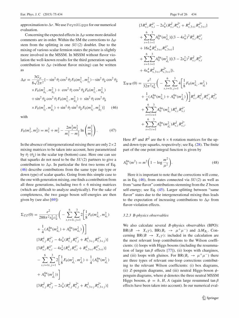
Table 1 Present experimentalstatus of B-physics observableswith their SM prediction

Observable Experimental value SM prediction

BR(B → Xsγ ) 3.43 ± 0.22 × 10−4 3.15 ± 0.23 × 10−4

BR(Bs → μ+μ−) (3.0)+1.0−0.9 × 10−9 3.23 ± 0.27 × 10−9

�MBs 116.4 ± 0.5 × 10−10 MeV (117.1)+17.2−16.4 × 10−10 MeV

0.002

0.0018

0.0016

0.00140.0012

0.001

1000 2000 3000 4000 50001000

1500

2000

2500

3000

m0 GeV

m12

GeV

tan 10, A0 0

0.0022

0.002

0.001

0.00160.00140.0012

1000 2000 3000 4000 50001000

1500

2000

2500

3000

m0 GeV

m12

GeV

tan 10, A0 3000

0.002

0.0018

0.0016

0.00140.0012

0.001

1000 2000 3000 4000 50001000

1500

2000

2500

3000

m0 GeV

m12

GeV

tan 45, A0 0

0.0022

0.002

0.0018

0.00160.0014

2000 3000 4000 50001000

1500

2000

2500

3000

m0 GeV

m12

GeV

tan 45, A0 3000

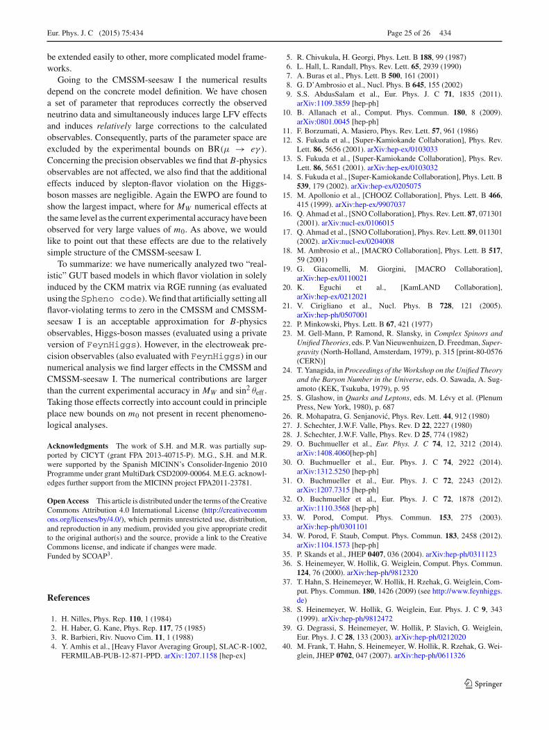
Fig. 1 Contours of δQLL13 in the m0–m1/2 plane for different values of tan β and A0 in the CMSSM

uation there are included what are known to be the dom-inant contributions to these three types of diagrams [78]:chargino contributions to box and Z -penguin diagrams, and

chargino and gluino contributions to φ-penguin diagrams.Concerning �MBs , in the MSSM there are in general threetypes of one-loop diagrams that contribute: (i) box diagrams,

123

Eur. Phys. J. C (2015) 75:434 Page 11 of 26 434

0.006 0.007 0.008 0.009 0.01

0.011

0.012

0.013

0.014

1000 2000 3000 4000 50001000

1500

2000

2500

3000

m0 GeV

m12

GeV

tan 10, A0 0

0.0090.01

0.011

0.012

0.013

0.014

0.015

1000 2000 3000 4000 50001000

1500

2000

2500

3000

m0 GeV

m12

GeV

tan 10, A0 3000

0.0060.007 0.008 0.009 0.01

0.011

0.012

0.013

0.014

0.015

1000 2000 3000 4000 50001000

1500

2000

2500

3000

m0 GeV

m12

GeV

tan 45, A0 0

0.009 0.01 0.011

0.012

0.013

0.014

0.015

0.016

2000 3000 4000 50001000

1500

2000

2500

3000

m0 GeV

m12

GeV

tan 45, A0 3000

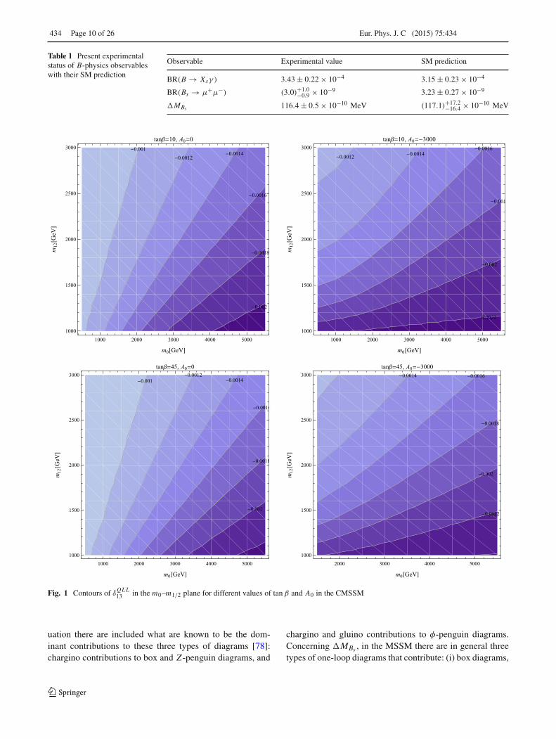
Fig. 2 Contours of δQLL23 in the m0–m1/2 plane for different values of tan β and A0 in the CMSSM

(ii) Z -penguin diagrams, and (iii) double Higgs-penguindiagrams (again including the resummation of large tan β

enhanced effects). In our numerical evaluation there areincluded again what are known to be the dominant contri-butions to these three types of diagrams in scenarios withnon-minimal flavor violation (for a review see, for instance,[79]): gluino contributions to box diagrams, chargino contri-butions to box and Z -penguin diagrams, and chargino and

gluino contributions to double φ-penguin diagrams. Moredetails about the calculations employed can be found in[44–46]. We perform our numerical calculation with theBPHYSICS subroutine taken from the SuFla code [42,43](with some additions and improvements as detailed in [44–46]), which has been implemented as a subroutine into (aprivate version of) FeynHiggs. The present experimentalstatus and SM prediction of these observables is given inTable 1 [80–87].

123

434 Page 12 of 26 Eur. Phys. J. C (2015) 75:434

1.6 10 6

2.5 10 6

3.3 10 64.2 10 6

5. 10 6

1000 2000 3000 4000 50001000

1500

2000

2500

3000

m0 GeV

m12

GeV

tan 10, A0 0

4. 10 68. 10 6

0.0000120.000016

1000 2000 3000 4000 50001000

1500

2000

2500

3000

m0 GeV

m12

GeV

tan 10, A0 3000

0.000029

0.000044

0.000059

0.000075

1000 2000 3000 4000 50001000

1500

2000

2500

3000

m0 GeV

m12

GeV

tan 45, A0 0

0.00007

0.00011

0.00015

2000 3000 4000 50001000

1500

2000

2500

3000

m0 GeV

m12

GeV

tan 45, A0 3000

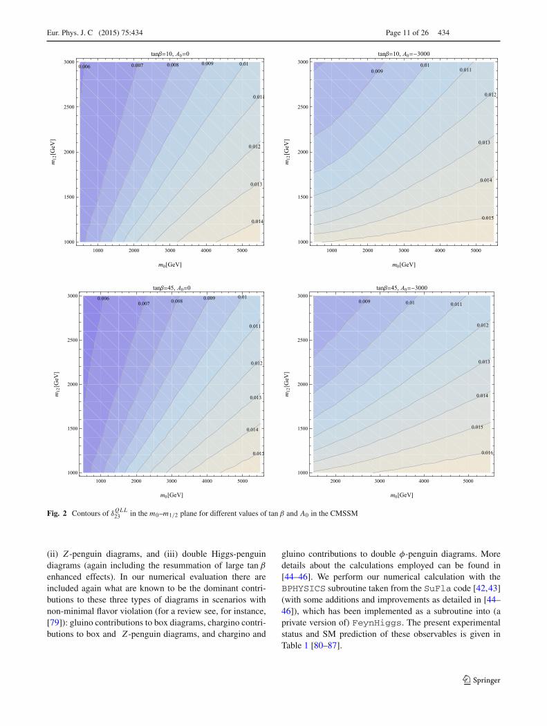
Fig. 3 Contours of δULR23 in the m0–m1/2 plane for different values of tan β and A0 in the CMSSM

4 Numerical results

4.1 Effects of squark mixing in the CMSSM

In this section we analyze the effects from RGE inducedflavor-violating mixing in the scalar quark sector in theCMSSM (i.e. with no mixing in the slepton sector). The RGErunning from the GUT scale to the EW has been performedas described in Sect. 3.1, with the subsequent evaluation of

the low-energy observables as discussed in Sect. 3.2. In orderto get an overview of the size of the effects in the CMSSMparameter space, the relevant parameters m0,m1/2 have beenscanned as (or in the case of A0 and tan β have been set to)all combinations of

m0 = 500 GeV . . . 5000 GeV, (49)

m1/2 = 1000 GeV . . . 3000 GeV, (50)

A0 = −3000,−2000,−1000, 0 GeV, (51)

123

Eur. Phys. J. C (2015) 75:434 Page 13 of 26 434

0.0002 0.0004 0.00060.0008 0.0011

1000 2000 3000 4000 50001000

1500

2000

2500

3000

m0 GeV

m12

GeV

tan 10, A0 0

0.0004 0.00060.0008

0.0011

0.0013

1000 2000 3000 4000 50001000

1500

2000

2500

3000

m0 GeV

m12

GeV

tan 10, A0 3000

0.0004 0.00090.0013 0.0018

0.0023

1000 2000 3000 4000 50001000

1500

2000

2500

3000

m0 GeV

m12

GeV

tan 45, A0 0

0.00090.0013

0.0016 0.0019 0.0023 0.0026

0.002

2000 3000 4000 50001000

1500

2000

2500

3000

m0 GeV

m12

GeV

tan 45, A0 3000

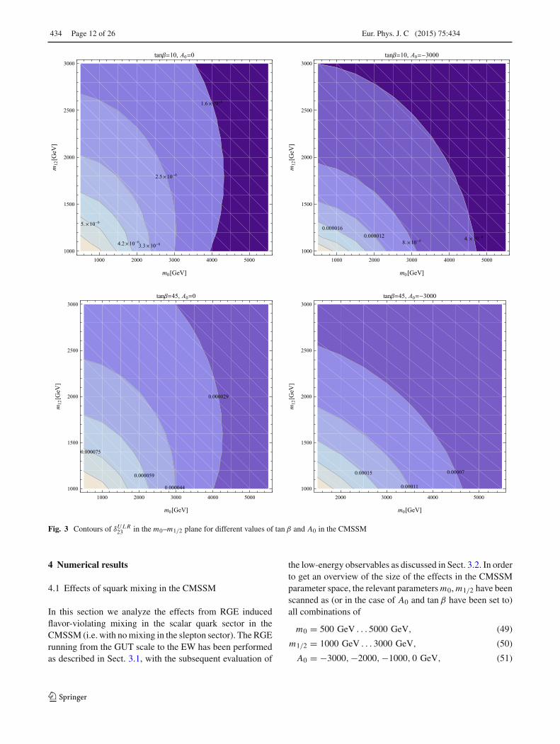
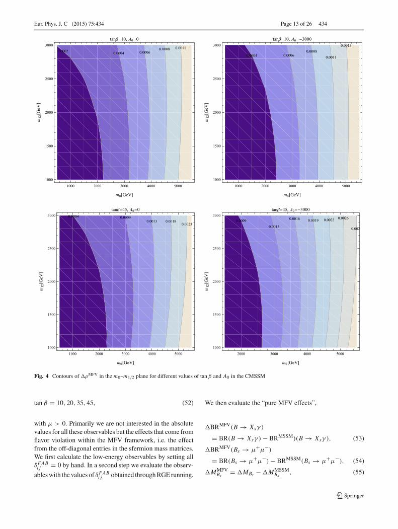
Fig. 4 Contours of �ρMFV in the m0–m1/2 plane for different values of tan β and A0 in the CMSSM

tan β = 10, 20, 35, 45, (52)

with μ > 0. Primarily we are not interested in the absolutevalues for all these observables but the effects that come fromflavor violation within the MFV framework, i.e. the effectfrom the off-diagonal entries in the sfermion mass matrices.We first calculate the low-energy observables by setting allδFABi j = 0 by hand. In a second step we evaluate the observ-

ables with the values of δFABi j obtained through RGE running.

We then evaluate the “pure MFV effects”,

�BRMFV(B → Xsγ )

= BR(B → Xsγ ) − BRMSSM)(B → Xsγ ), (53)

�BRMFV(Bs → μ+μ−)

= BR(Bs → μ+μ−) − BRMSSM(Bs → μ+μ−), (54)

�MMFVBs = �MBs − �MMSSM

Bs , (55)

123

434 Page 14 of 26 Eur. Phys. J. C (2015) 75:434

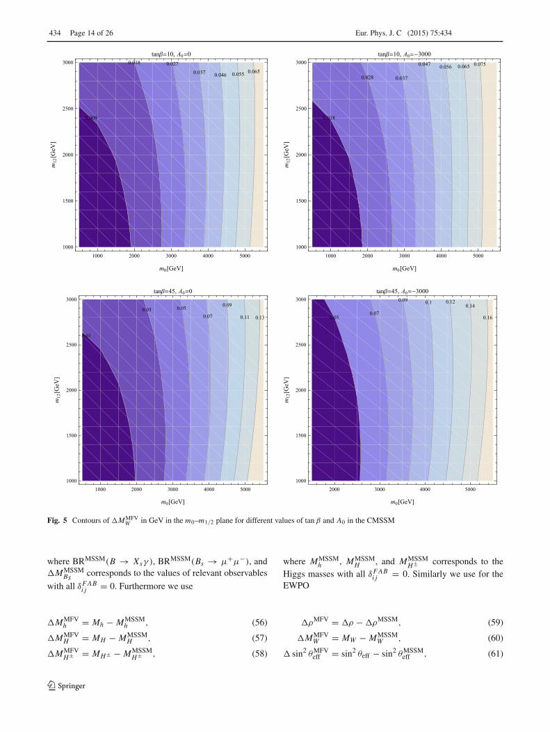
0.009

0.018 0.0270.037 0.046 0.055 0.065

1000 2000 3000 4000 50001000

1500

2000

2500

3000

m0 GeV

m12

GeV

tan 10, A0 0

0.018

0.028 0.037

0.047 0.056 0.065 0.075

1000 2000 3000 4000 50001000

1500

2000

2500

3000

m0 GeV

m12

GeV

tan 10, A0 3000

0.01

0.03 0.050.07

0.09

0.11 0.13

1000 2000 3000 4000 50001000

1500

2000

2500

3000

m0 GeV

m12

GeV

tan 45, A0 0

0.050.07

0.09 0.1 0.120.14

0.16

2000 3000 4000 50001000

1500

2000

2500

3000

m0 GeV

m12

GeV

tan 45, A0 3000

Fig. 5 Contours of �MMFVW in GeV in the m0–m1/2 plane for different values of tan β and A0 in the CMSSM

where BRMSSM(B → Xsγ ), BRMSSM(Bs → μ+μ−), and�MMSSM

BScorresponds to the values of relevant observables

with all δFABi j = 0. Furthermore we use

�MMFVh = Mh − MMSSM

h , (56)

�MMFVH = MH − MMSSM

H , (57)

�MMFVH± = MH± − MMSSM

H± , (58)

where MMSSMh , MMSSM

H , and MMSSMH± corresponds to the

Higgs masses with all δFABi j = 0. Similarly we use for the

EWPO

�ρMFV = �ρ − �ρMSSM, (59)

�MMFVW = MW − MMSSM

W , (60)

� sin2 θMFVeff = sin2 θeff − sin2 θMSSM

eff , (61)

123

Eur. Phys. J. C (2015) 75:434 Page 15 of 26 434

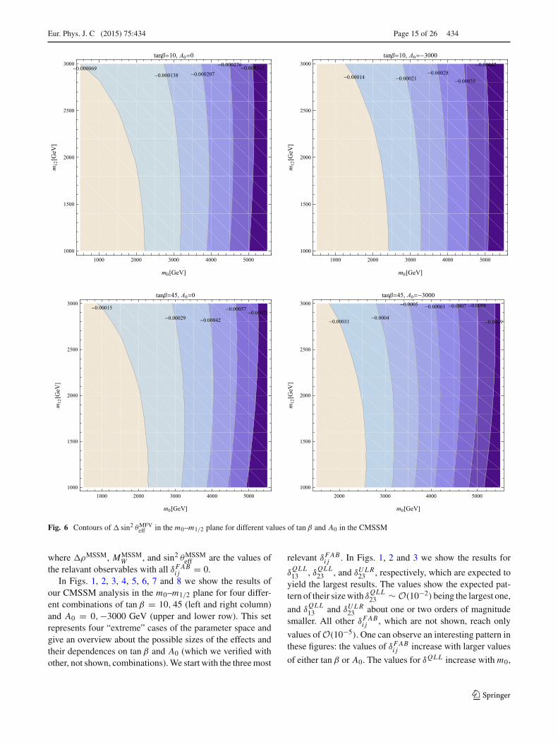
0.0003450.000276

0.0002070.0001380.000069

1000 2000 3000 4000 50001000

1500

2000

2500

3000

m0 GeV

m12

GeV

tan 10, A0 00.00042

0.000350.00028

0.000210.00014

1000 2000 3000 4000 50001000

1500

2000

2500

3000

m0 GeV

m12

GeV

tan 10, A0 3000

0.000710.00057

0.000420.00029

0.00015

1000 2000 3000 4000 50001000

1500

2000

2500

3000

m0 GeV

m12

GeV

tan 45, A0 0

0.00091

0.00080.00070.000610.0005

0.00040.00031

2000 3000 4000 50001000

1500

2000

2500

3000

m0 GeV

m12

GeV

tan 45, A0 3000

Fig. 6 Contours of � sin2 θMFVeff in the m0–m1/2 plane for different values of tan β and A0 in the CMSSM

where �ρMSSM, MMSSMW , and sin2 θMSSM

eff are the values ofthe relavant observables with all δFAB

i j = 0.In Figs. 1, 2, 3, 4, 5, 6, 7 and 8 we show the results of

our CMSSM analysis in the m0–m1/2 plane for four differ-ent combinations of tan β = 10, 45 (left and right column)and A0 = 0,−3000 GeV (upper and lower row). This setrepresents four “extreme” cases of the parameter space andgive an overview about the possible sizes of the effects andtheir dependences on tan β and A0 (which we verified withother, not shown, combinations). We start with the three most

relevant δFABi j . In Figs. 1, 2 and 3 we show the results for

δQLL13 , δ

QLL23 , and δULR

23 , respectively, which are expected toyield the largest results. The values show the expected pat-tern of their size with δ

QLL23 ∼ O(10−2) being the largest one,

and δQLL13 and δULR

23 about one or two orders of magnitudesmaller. All other δFAB

i j , which are not shown, reach only

values of O(10−5). One can observe an interesting pattern inthese figures: the values of δFAB

i j increase with larger values

of either tan β or A0. The values for δQLL increase with m0,

123

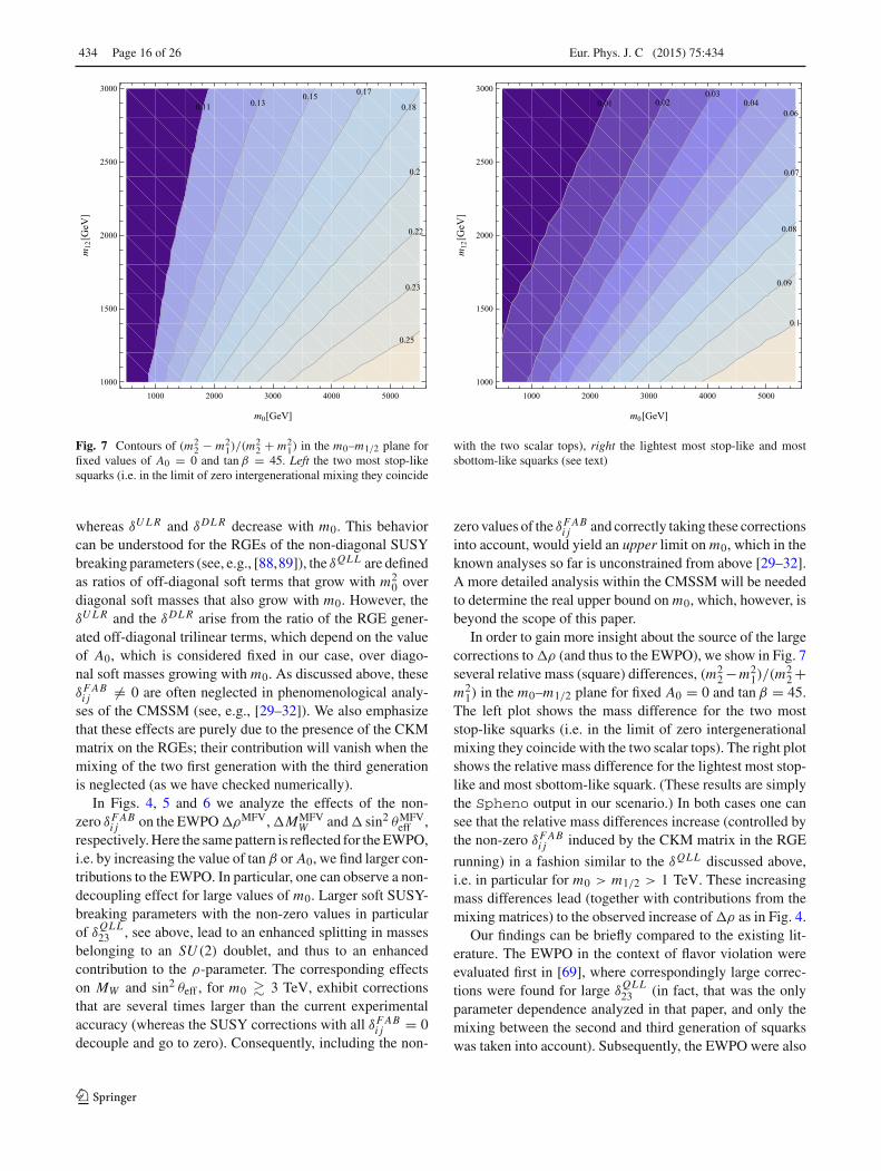
434 Page 16 of 26 Eur. Phys. J. C (2015) 75:434

0.11 0.130.15 0.17

0.18

0.2

0.22

0.23

0.25

1000 2000 3000 4000 50001000

1500

2000

2500

3000

m0 GeV

m12

GeV

0.01 0.020.03

0.040.06

0.07

0.08

0.09

0.1

1000 2000 3000 4000 50001000

1500

2000

2500

3000

m0 GeV

m12

GeV

Fig. 7 Contours of (m22 − m2

1)/(m22 + m2

1) in the m0–m1/2 plane forfixed values of A0 = 0 and tan β = 45. Left the two most stop-likesquarks (i.e. in the limit of zero intergenerational mixing they coincide

with the two scalar tops), right the lightest most stop-like and mostsbottom-like squarks (see text)

whereas δULR and δDLR decrease with m0. This behaviorcan be understood for the RGEs of the non-diagonal SUSYbreaking parameters (see, e.g., [88,89]), the δQLL are definedas ratios of off-diagonal soft terms that grow with m2

0 overdiagonal soft masses that also grow with m0. However, theδULR and the δDLR arise from the ratio of the RGE gener-ated off-diagonal trilinear terms, which depend on the valueof A0, which is considered fixed in our case, over diago-nal soft masses growing with m0. As discussed above, theseδFABi j �= 0 are often neglected in phenomenological analy-

ses of the CMSSM (see, e.g., [29–32]). We also emphasizethat these effects are purely due to the presence of the CKMmatrix on the RGEs; their contribution will vanish when themixing of the two first generation with the third generationis neglected (as we have checked numerically).

In Figs. 4, 5 and 6 we analyze the effects of the non-zero δFAB

i j on the EWPO �ρMFV, �MMFVW and � sin2 θMFV

eff ,respectively. Here the same pattern is reflected for the EWPO,i.e. by increasing the value of tan β or A0, we find larger con-tributions to the EWPO. In particular, one can observe a non-decoupling effect for large values of m0. Larger soft SUSY-breaking parameters with the non-zero values in particularof δ

QLL23 , see above, lead to an enhanced splitting in masses

belonging to an SU (2) doublet, and thus to an enhancedcontribution to the ρ-parameter. The corresponding effectson MW and sin2 θeff , for m0 � 3 TeV, exhibit correctionsthat are several times larger than the current experimentalaccuracy (whereas the SUSY corrections with all δFAB

i j = 0decouple and go to zero). Consequently, including the non-

zero values of the δFABi j and correctly taking these corrections

into account, would yield an upper limit on m0, which in theknown analyses so far is unconstrained from above [29–32].A more detailed analysis within the CMSSM will be neededto determine the real upper bound on m0, which, however, isbeyond the scope of this paper.

In order to gain more insight about the source of the largecorrections to �ρ (and thus to the EWPO), we show in Fig. 7several relative mass (square) differences, (m2

2 −m21)/(m

22 +

m21) in the m0–m1/2 plane for fixed A0 = 0 and tan β = 45.

The left plot shows the mass difference for the two moststop-like squarks (i.e. in the limit of zero intergenerationalmixing they coincide with the two scalar tops). The right plotshows the relative mass difference for the lightest most stop-like and most sbottom-like squark. (These results are simplythe Spheno output in our scenario.) In both cases one cansee that the relative mass differences increase (controlled bythe non-zero δFAB

i j induced by the CKM matrix in the RGE

running) in a fashion similar to the δQLL discussed above,i.e. in particular for m0 > m1/2 > 1 TeV. These increasingmass differences lead (together with contributions from themixing matrices) to the observed increase of �ρ as in Fig. 4.

Our findings can be briefly compared to the existing lit-erature. The EWPO in the context of flavor violation wereevaluated first in [69], where correspondingly large correc-tions were found for large δ

QLL23 (in fact, that was the only

parameter dependence analyzed in that paper, and only themixing between the second and third generation of squarkswas taken into account). Subsequently, the EWPO were also

123

Eur. Phys. J. C (2015) 75:434 Page 17 of 26 434

0.0000390.000026

0.000013

2000 3000 4000 50001000

1500

2000

2500

3000

m0 GeV

m12

GeV

tan 45, A0 3000

0.0000390.000026

0.000013

2000 3000 4000 50001000

1500

2000

2500

3000

m0 GeV

m12

GeV

tan 45, A0 3000

0.26

0.23

0.2

0.16

0.13

2000 3000 4000 50001000

1500

2000

2500

3000

m0 GeV

m12

GeV

MHMFV

7. 10 6 6. 10 6 5. 10 6

4. 10 6

3. 10 6

2. 10 6

2000 3000 4000 50001000

1500

2000

2500

3000

m0 GeV

m12

GeV

BRMFV B Xs

4.8 10 10

3.6 10 10

2.4 10 10

1.2 10 10

2000 3000 4000 50001000

1500

2000

2500

3000

m0 GeV

m12

GeV

BRMFV Bs

3. 10 15

6. 10 151. 10 14

1.3 10 14

2000 3000 4000 50001000

1500

2000

2500

3000

m0 GeV

m12

GeV

MBMFV

Fig. 8 Contours of Higgs mass corrections (�MMFVh , �MMFV

H and �MMFVH± in GeV) and BPO (�BRMFV(B → Xsγ ), �BRMFV(Bs → μ+μ−)

and �MMFVBs

) in the m0–m1/2 plane for tan β = 45 and A0 = −3000 GeV in the CMSSM

123

434 Page 18 of 26 Eur. Phys. J. C (2015) 75:434

0.001

0.0010.0008

0.000610.0004

1000 2000 3000 4000 50001000

1500

2000

2500

3000

m0 GeV

m12

GeV

tan 10, A0 0

0.0042

0.0035

0.0028

0.0021

0.0014

1000 2000 3000 4000 50001000

1500

2000

2500

3000

m0 GeV

m12

GeV

tan 10, A0 3000

0.00121

0.0010.00080.00061

0.0004

1000 2000 3000 4000 50001000

1500

2000

2500

3000

m0 GeV

m12

GeV

tan 45, A0 0

0.0024

0.0021

0.0017

0.0014

2000 3000 4000 50001000

1500

2000

2500

3000

m0 GeV

m12

GeV

tan 45, A0 3000

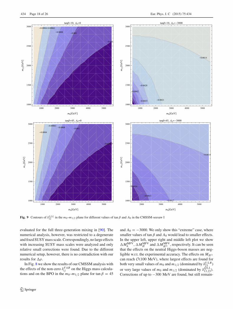
Fig. 9 Contours of δLLL12 in the m0–m1/2 plane for different values of tan β and A0 in the CMSSM-seesaw I

evaluated for the full three-generation mixing in [90]. Thenumerical analysis, however, was restricted to a degenerateand fixed SUSY mass scale. Correspondingly, no large effectswith increasing SUSY mass scales were analyzed and onlyrelative small corrections were found. Due to the differentnumerical setup, however, there is no contradiction with ourresults for �ρ.

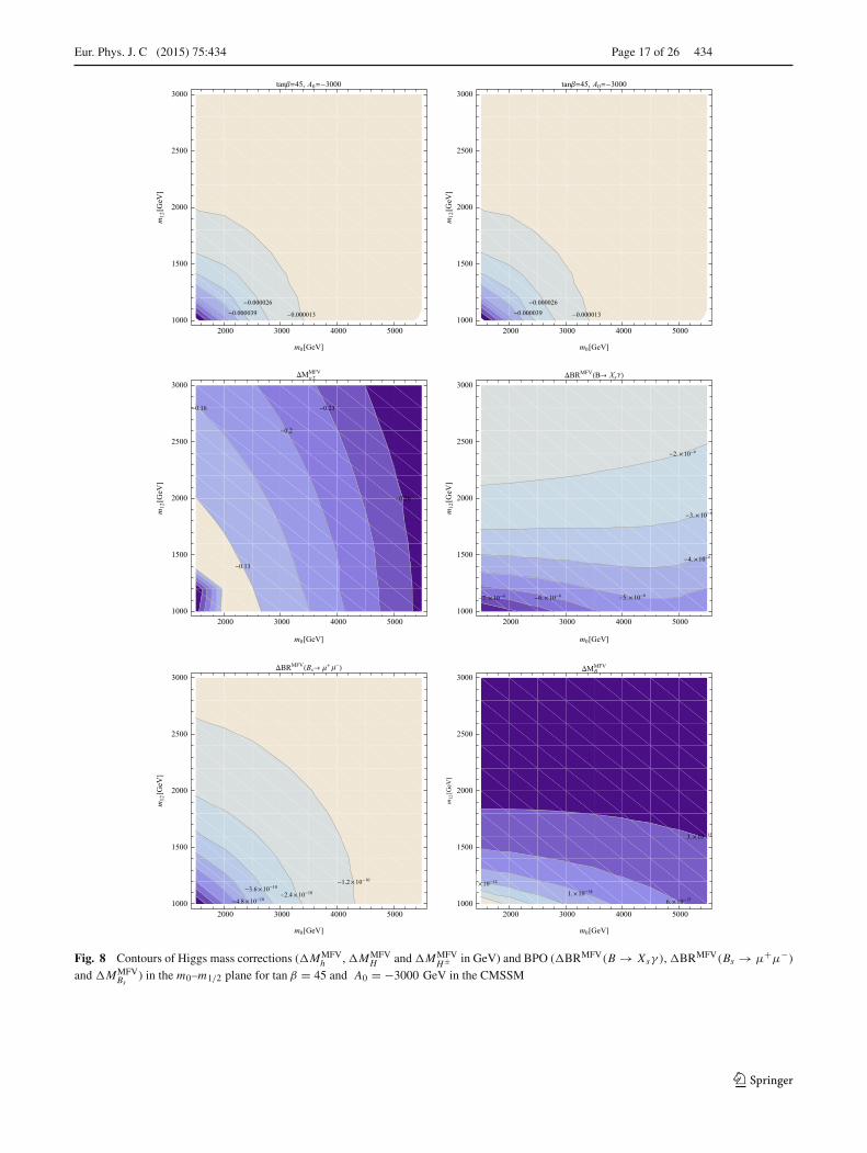
In Fig. 8 we show the results of our CMSSM analysis withthe effects of the non-zero δFAB

i j on the Higgs mass calcula-tions and on the BPO in the m0–m1/2 plane for tan β = 45

and A0 = −3000. We only show this “extreme” case, wheresmaller values of tan β and A0 would lead to smaller effects.In the upper left, upper right and middle left plot we show�MMFV

h , �MMFVH and �MMFV

H± , respectively. It can be seenthat the effects on the neutral Higgs-boson masses are neg-ligible w.r.t. the experimental accuracy. The effects on MH±can reach O(100 MeV), where largest effects are found forboth very small values of m0 and m1/2 (dominated by δULR

23 )

or very large values of m0 and m1/2 (dominated by δQLL13,23).

Corrections of up to −300 MeV are found, but still remain-

123

Eur. Phys. J. C (2015) 75:434 Page 19 of 26 434

0.0012

0.0010.0008

0.000610.0004

1000 2000 3000 4000 50001000

1500

2000

2500

3000

m0 GeV

m12

GeV

tan 10, A0 0

0.00420.0035

0.0028

0.0021

0.0014

1000 2000 3000 4000 50001000

1500

2000

2500

3000

m0 GeV

m12

GeV

tan 10, A0 3000

0.00126

0.001060.00084

0.00063

0.00042

1000 2000 3000 4000 50001000

1500

2000

2500

3000

m0 GeV

m12

GeV

tan 45, A0 0

0.0026

0.00230.0019

0.0015

2000 3000 4000 50001000

1500

2000

2500

3000

m0 GeV

m12

GeV

tan 45, A0 3000

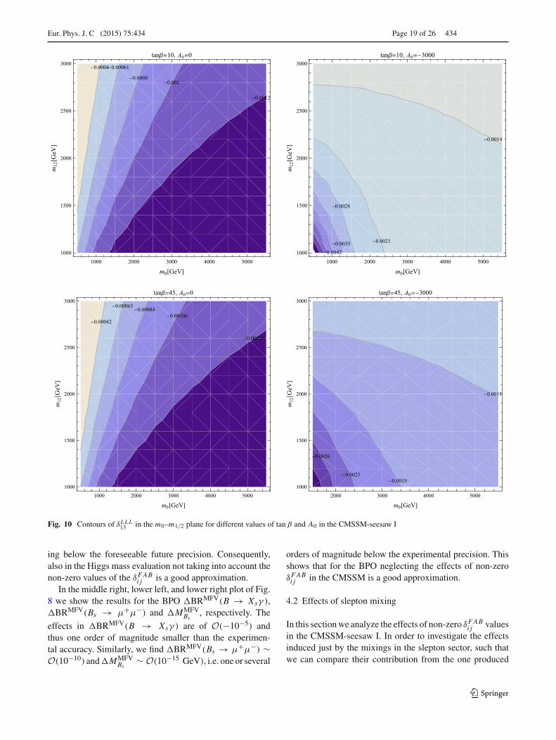
Fig. 10 Contours of δLLL13 in the m0–m1/2 plane for different values of tan β and A0 in the CMSSM-seesaw I

ing below the foreseeable future precision. Consequently,also in the Higgs mass evaluation not taking into account thenon-zero values of the δFAB

i j is a good approximation.In the middle right, lower left, and lower right plot of Fig.

8 we show the results for the BPO �BRMFV(B → Xsγ ),�BRMFV(Bs → μ+μ−) and �MMFV

Bs, respectively. The

effects in �BRMFV(B → Xsγ ) are of O(−10−5) andthus one order of magnitude smaller than the experimen-tal accuracy. Similarly, we find �BRMFV(Bs → μ+μ−) ∼O(10−10) and �MMFV

Bs∼ O(10−15 GeV), i.e. one or several

orders of magnitude below the experimental precision. Thisshows that for the BPO neglecting the effects of non-zeroδFABi j in the CMSSM is a good approximation.

4.2 Effects of slepton mixing

In this section we analyze the effects of non-zero δFABi j values

in the CMSSM-seesaw I. In order to investigate the effectsinduced just by the mixings in the slepton sector, such thatwe can compare their contribution from the one produced

123

434 Page 20 of 26 Eur. Phys. J. C (2015) 75:434

0.003 0.005

0.0060.008

0.01

1000 2000 3000 4000 50001000

1500

2000

2500

3000

m0 GeV

m12

GeV

tan 10, A0 0

0.013

0.019

0.026

0.033

1000 2000 3000 4000 50001000

1500

2000

2500

3000

m0 GeV

m12

GeV

tan 10, A0 3000

0.0020.004 0.005 0.007

0.0080.009

0.011

1000 2000 3000 4000 50001000

1500

2000

2500

3000

m0 GeV

m12

GeV

tan 45, A0 0

0.013

0.0160.019

0.023

2000 3000 4000 50001000

1500

2000

2500

3000

m0 GeV

m12

GeV

tan 45, A0 3000

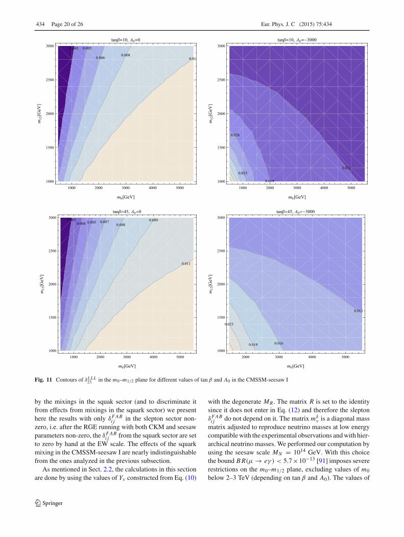
Fig. 11 Contours of δLLL23 in the m0–m1/2 plane for different values of tan β and A0 in the CMSSM-seesaw I

by the mixings in the squak sector (and to discriminate itfrom effects from mixings in the squark sector) we presenthere the results with only δFAB

i j in the slepton sector non-zero, i.e. after the RGE running with both CKM and seesawparameters non-zero, the δFAB

i j from the squark sector are setto zero by hand at the EW scale. The effects of the squarkmixing in the CMSSM-seesaw I are nearly indistinguishablefrom the ones analyzed in the previous subsection.

As mentioned in Sect. 2.2, the calculations in this sectionare done by using the values of Yν constructed from Eq. (10)

with the degenerate MR . The matrix R is set to the identitysince it does not enter in Eq. (12) and therefore the sleptonδFABi j do not depend on it. The matrix mδ

ν is a diagonal massmatrix adjusted to reproduce neutrino masses at low energycompatible with the experimental observations and with hier-archical neutrino masses. We performed our computation byusing the seesaw scale MN = 1014 GeV. With this choicethe bound BR(μ → eγ ) < 5.7×10−13 [91] imposes severerestrictions on the m0–m1/2 plane, excluding values of m0

below 2–3 TeV (depending on tan β and A0). The values of

123

Eur. Phys. J. C (2015) 75:434 Page 21 of 26 434

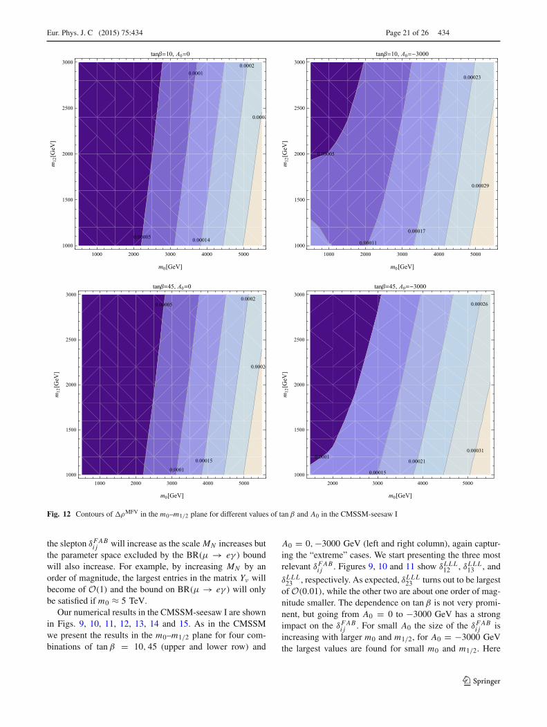
0.00005

0.0001

0.00014

0.0002

0.0002

1000 2000 3000 4000 50001000

1500

2000

2500

3000

m0 GeV

m12

GeV

tan 10, A0 0

0.00005

0.00011

0.00017

0.00023

0.00029

1000 2000 3000 4000 50001000

1500

2000

2500

3000

m0 GeV

m12

GeV

tan 10, A0 3000

0.00005

0.0001

0.00015

0.0002

0.0002

1000 2000 3000 4000 50001000

1500

2000

2500

3000

m0 GeV

m12

GeV

tan 45, A0 0

0.0001

0.00015

0.00021

0.00026

0.00031

2000 3000 4000 50001000

1500

2000

2500

3000

m0 GeV

m12

GeV

tan 45, A0 3000

Fig. 12 Contours of �ρMFV in the m0–m1/2 plane for different values of tan β and A0 in the CMSSM-seesaw I

the slepton δFABi j will increase as the scale MN increases but

the parameter space excluded by the BR(μ → eγ ) boundwill also increase. For example, by increasing MN by anorder of magnitude, the largest entries in the matrix Yν willbecome of O(1) and the bound on BR(μ → eγ ) will onlybe satisfied if m0 ≈ 5 TeV.

Our numerical results in the CMSSM-seesaw I are shownin Figs. 9, 10, 11, 12, 13, 14 and 15. As in the CMSSMwe present the results in the m0–m1/2 plane for four com-binations of tan β = 10, 45 (upper and lower row) and

A0 = 0,−3000 GeV (left and right column), again captur-ing the “extreme” cases. We start presenting the three mostrelevant δFAB

i j . Figures 9, 10 and 11 show δLLL12 , δLLL13 , and

δLLL23 , respectively. As expected, δLLL23 turns out to be largestof O(0.01), while the other two are about one order of mag-nitude smaller. The dependence on tan β is not very promi-nent, but going from A0 = 0 to −3000 GeV has a strongimpact on the δFAB

i j . For small A0 the size of the δFABi j is

increasing with larger m0 and m1/2, for A0 = −3000 GeVthe largest values are found for small m0 and m1/2. Here

123

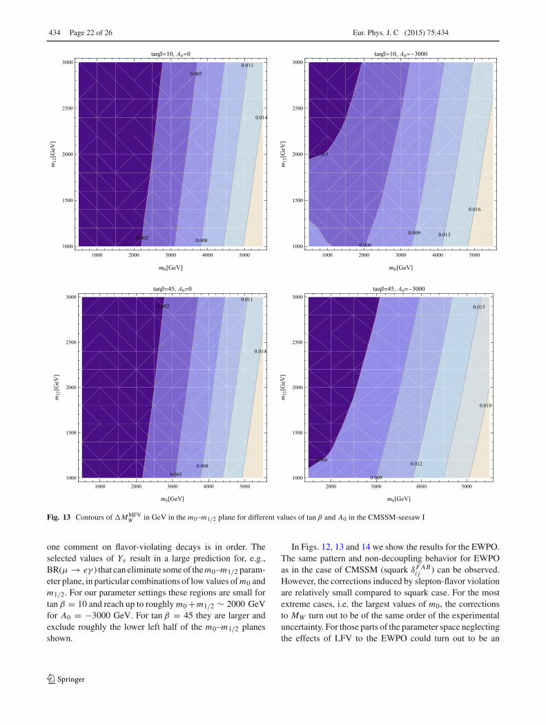
434 Page 22 of 26 Eur. Phys. J. C (2015) 75:434

0.002

0.005

0.008

0.011

0.014

1000 2000 3000 4000 50001000

1500

2000

2500

3000

m0 GeV

m12

GeV

tan 10, A0 0

0.003

0.006

0.009 0.013

0.016

1000 2000 3000 4000 50001000

1500

2000

2500

3000

m0 GeV

m12

GeV

tan 10, A0 3000

0.002

0.0050.008

0.011

0.014

1000 2000 3000 4000 50001000

1500

2000

2500

3000

m0 GeV

m12

GeV

tan 45, A0 0

0.006

0.009

0.012

0.015

0.018

2000 3000 4000 50001000

1500

2000

2500

3000

m0 GeV

m12

GeV

tan 45, A0 3000

Fig. 13 Contours of �MMFVW in GeV in the m0–m1/2 plane for different values of tan β and A0 in the CMSSM-seesaw I

one comment on flavor-violating decays is in order. Theselected values of Yν result in a large prediction for, e.g.,BR(μ → eγ ) that can eliminate some of them0–m1/2 param-eter plane, in particular combinations of low values ofm0 andm1/2. For our parameter settings these regions are small fortan β = 10 and reach up to roughly m0 +m1/2 ∼ 2000 GeVfor A0 = −3000 GeV. For tan β = 45 they are larger andexclude roughly the lower left half of the m0–m1/2 planesshown.

In Figs. 12, 13 and 14 we show the results for the EWPO.The same pattern and non-decoupling behavior for EWPOas in the case of CMSSM (squark δFAB

i j ) can be observed.However, the corrections induced by slepton-flavor violationare relatively small compared to squark case. For the mostextreme cases, i.e. the largest values of m0, the correctionsto MW turn out to be of the same order of the experimentaluncertainty. For those parts of the parameter space neglectingthe effects of LFV to the EWPO could turn out to be an

123

Eur. Phys. J. C (2015) 75:434 Page 23 of 26 434

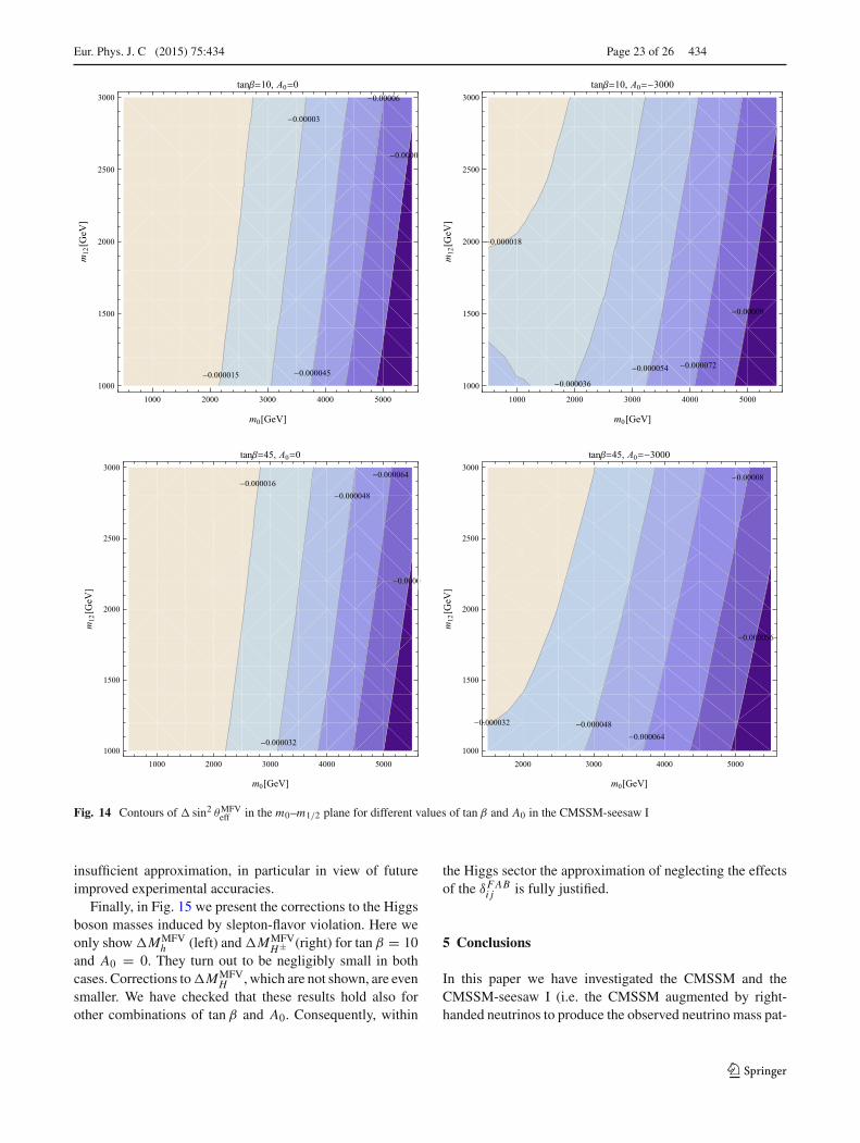
0.0000

0.00006

0.000045

0.00003

0.000015

1000 2000 3000 4000 50001000

1500

2000

2500

3000

m0 GeV

m12

GeV

tan 10, A0 0

0.00009

0.0000720.000054

0.000036

0.000018

1000 2000 3000 4000 50001000

1500

2000

2500

3000

m0 GeV

m12

GeV

tan 10, A0 3000

0.0000

0.000064

0.000048

0.000032

0.000016

1000 2000 3000 4000 50001000

1500

2000

2500

3000

m0 GeV

m12

GeV

tan 45, A0 0

0.000096

0.00008

0.0000640.0000480.000032

2000 3000 4000 50001000

1500

2000

2500

3000

m0 GeV

m12

GeV

tan 45, A0 3000

Fig. 14 Contours of � sin2 θMFVeff in the m0–m1/2 plane for different values of tan β and A0 in the CMSSM-seesaw I

insufficient approximation, in particular in view of futureimproved experimental accuracies.

Finally, in Fig. 15 we present the corrections to the Higgsboson masses induced by slepton-flavor violation. Here weonly show �MMFV

h (left) and �MMFVH± (right) for tan β = 10

and A0 = 0. They turn out to be negligibly small in bothcases. Corrections to �MMFV

H , which are not shown, are evensmaller. We have checked that these results hold also forother combinations of tan β and A0. Consequently, within

the Higgs sector the approximation of neglecting the effectsof the δFAB

i j is fully justified.

5 Conclusions

In this paper we have investigated the CMSSM and theCMSSM-seesaw I (i.e. the CMSSM augmented by right-handed neutrinos to produce the observed neutrino mass pat-

123

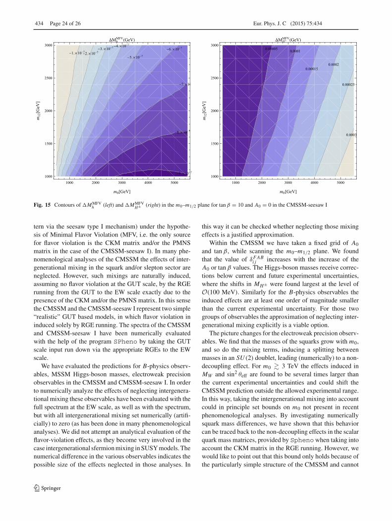
434 Page 24 of 26 Eur. Phys. J. C (2015) 75:434

9. 10 7

8. 10 7

7. 10

6. 10 7

5. 10 7

4. 10 73. 10 7

2. 10 71. 10 7

1000 2000 3000 4000 50001000

1500

2000

2500

3000

m0 GeV

m12

GeV

MhMFV GeV

0.00005 0.0001

0.000150.0002

0.00025

0.0003

1000 2000 3000 4000 50001000

1500

2000

2500

3000

m0 GeV

m12

GeV

MHMFV GeV

Fig. 15 Contours of �MMFVh (left) and �MMFV

H± (right) in the m0–m1/2 plane for tan β = 10 and A0 = 0 in the CMSSM-seesaw I

tern via the seesaw type I mechanism) under the hypothe-sis of Minimal Flavor Violation (MFV, i.e. the only sourcefor flavor violation is the CKM matrix and/or the PMNSmatrix in the case of the CMSSM-seesaw I). In many phe-nomenological analyses of the CMSSM the effects of inter-generational mixing in the squark and/or slepton sector areneglected. However, such mixings are naturally induced,assuming no flavor violation at the GUT scale, by the RGErunning from the GUT to the EW scale exactly due to thepresence of the CKM and/or the PMNS matrix. In this sensethe CMSSM and the CMSSM-seesaw I represent two simple“realistic” GUT based models, in which flavor violation ininduced solely by RGE running. The spectra of the CMSSMand CMSSM-seesaw I have been numerically evaluatedwith the help of the program SPheno by taking the GUTscale input run down via the appropriate RGEs to the EWscale.

We have evaluated the predictions for B-physics observ-ables, MSSM Higgs-boson masses, electroweak precisionobservables in the CMSSM and CMSSM-seesaw I. In orderto numerically analyze the effects of neglecting intergenera-tional mixing these observables have been evaluated with thefull spectrum at the EW scale, as well as with the spectrum,but with all intergenerational mixing set numerically (artifi-cially) to zero (as has been done in many phenomenologicalanalyses). We did not attempt an analytical evaluation of theflavor-violation effects, as they become very involved in thecase intergenerational sfermion mixing in SUSY models. Thenumerical difference in the various observables indicates thepossible size of the effects neglected in those analyses. In

this way it can be checked whether neglecting those mixingeffects is a justified approximation.

Within the CMSSM we have taken a fixed grid of A0

and tan β, while scanning the m0–m1/2 plane. We foundthat the value of δFAB

i j increases with the increase of theA0 or tan β values. The Higgs-boson masses receive correc-tions below current and future experimental uncertainties,where the shifts in MH± were found largest at the level ofO(100 MeV). Similarly for the B-physics observables theinduced effects are at least one order of magnitude smallerthan the current experimental uncertainty. For those twogroups of observables the approximation of neglecting inter-generational mixing explicitly is a viable option.

The picture changes for the electroweak precision observ-ables. We find that the masses of the squarks grow with m0,and so do the mixing terms, inducing a splitting betweenmasses in an SU (2) doublet, leading (numerically) to a non-decoupling effect. For m0 � 3 TeV the effects induced inMW and sin2 θeff are found to be several times larger thanthe current experimental uncertainties and could shift theCMSSM prediction outside the allowed experimental range.In this way, taking the intergenerational mixing into accountcould in principle set bounds on m0 not present in recentphenomenological analyses. By investigating numericallysquark mass differences, we have shown that this behaviorcan be traced back to the non-decoupling effects in the scalarquark mass matrices, provided by Spheno when taking intoaccount the CKM matrix in the RGE running. However, wewould like to point out that this bound only holds because ofthe particularly simple structure of the CMSSM and cannot

123

Eur. Phys. J. C (2015) 75:434 Page 25 of 26 434

be extended easily to other, more complicated model frame-works.

Going to the CMSSM-seesaw I the numerical resultsdepend on the concrete model definition. We have chosena set of parameter that reproduces correctly the observedneutrino data and simultaneously induces large LFV effectsand induces relatively large corrections to the calculatedobservables. Consequently, parts of the parameter space areexcluded by the experimental bounds on BR(μ → eγ ).Concerning the precision observables we find that B-physicsobservables are not affected, we also find that the additionaleffects induced by slepton-flavor violation on the Higgs-boson masses are negligible. Again the EWPO are found toshow the largest impact, where for MW numerical effects atthe same level as the current experimental accuracy have beenobserved for very large values of m0. As above, we wouldlike to point out that these effects are due to the relativelysimple structure of the CMSSM-seesaw I.

To summarize: we have numerically analyzed two “real-istic” GUT based models in which flavor violation in solelyinduced by the CKM matrix via RGE running (as evaluatedusing theSpheno code). We find that artificially setting allflavor-violating terms to zero in the CMSSM and CMSSM-seesaw I is an acceptable approximation for B-physicsobservables, Higgs-boson masses (evaluated using a privateversion of FeynHiggs). However, in the electroweak pre-cision observables (also evaluated with FeynHiggs) in ournumerical analysis we find larger effects in the CMSSM andCMSSM-seesaw I. The numerical contributions are largerthan the current experimental accuracy in MW and sin2 θeff .Taking those effects correctly into account could in principleplace new bounds on m0 not present in recent phenomeno-logical analyses.

Acknowledgments The work of S.H. and M.R. was partially sup-ported by CICYT (grant FPA 2013-40715-P). M.G., S.H. and M.R.were supported by the Spanish MICINN’s Consolider-Ingenio 2010Programme under grant MultiDark CSD2009-00064. M.E.G. acknowl-edges further support from the MICINN project FPA2011-23781.

OpenAccess This article is distributed under the terms of the CreativeCommons Attribution 4.0 International License (http://creativecommons.org/licenses/by/4.0/), which permits unrestricted use, distribution,and reproduction in any medium, provided you give appropriate creditto the original author(s) and the source, provide a link to the CreativeCommons license, and indicate if changes were made.Funded by SCOAP3.

References

1. H. Nilles, Phys. Rep. 110, 1 (1984)2. H. Haber, G. Kane, Phys. Rep. 117, 75 (1985)3. R. Barbieri, Riv. Nuovo Cim. 11, 1 (1988)4. Y. Amhis et al., [Heavy Flavor Averaging Group], SLAC-R-1002,

FERMILAB-PUB-12-871-PPD. arXiv:1207.1158 [hep-ex]

5. R. Chivukula, H. Georgi, Phys. Lett. B 188, 99 (1987)6. L. Hall, L. Randall, Phys. Rev. Lett. 65, 2939 (1990)7. A. Buras et al., Phys. Lett. B 500, 161 (2001)8. G. D’Ambrosio et al., Nucl. Phys. B 645, 155 (2002)9. S.S. AbdusSalam et al., Eur. Phys. J. C 71, 1835 (2011).

arXiv:1109.3859 [hep-ph]10. B. Allanach et al., Comput. Phys. Commun. 180, 8 (2009).

arXiv:0801.0045 [hep-ph]11. F. Borzumati, A. Masiero, Phys. Rev. Lett. 57, 961 (1986)12. S. Fukuda et al., [Super-Kamiokande Collaboration], Phys. Rev.

Lett. 86, 5656 (2001). arXiv:hep-ex/010303313. S. Fukuda et al., [Super-Kamiokande Collaboration], Phys. Rev.

Lett. 86, 5651 (2001). arXiv:hep-ex/010303214. S. Fukuda et al., [Super-Kamiokande Collaboration], Phys. Lett. B

539, 179 (2002). arXiv:hep-ex/020507515. M. Apollonio et al., [CHOOZ Collaboration], Phys. Lett. B 466,

415 (1999). arXiv:hep-ex/990703716. Q. Ahmad et al., [SNO Collaboration], Phys. Rev. Lett. 87, 071301

(2001). arXiv:nucl-ex/010601517. Q. Ahmad et al., [SNO Collaboration], Phys. Rev. Lett. 89, 011301

(2002). arXiv:nucl-ex/020400818. M. Ambrosio et al., [MACRO Collaboration], Phys. Lett. B 517,

59 (2001)19. G. Giacomelli, M. Giorgini, [MACRO Collaboration],

arXiv:hep-ex/011002120. K. Eguchi et al., [KamLAND Collaboration],

arXiv:hep-ex/021202121. V. Cirigliano et al., Nucl. Phys. B 728, 121 (2005).

arXiv:hep-ph/050700122. P. Minkowski, Phys. Lett. B 67, 421 (1977)23. M. Gell-Mann, P. Ramond, R. Slansky, in Complex Spinors and

Unified Theories, eds. P. Van Nieuwenhuizen, D. Freedman, Super-gravity (North-Holland, Amsterdam, 1979), p. 315 [print-80-0576(CERN)]

24. T. Yanagida, in Proceedings of theWorkshop on the Unified Theoryand the Baryon Number in the Universe, eds. O. Sawada, A. Sug-amoto (KEK, Tsukuba, 1979), p. 95

25. S. Glashow, in Quarks and Leptons, eds. M. Lévy et al. (PlenumPress, New York, 1980), p. 687

26. R. Mohapatra, G. Senjanovic, Phys. Rev. Lett. 44, 912 (1980)27. J. Schechter, J.W.F. Valle, Phys. Rev. D 22, 2227 (1980)28. J. Schechter, J.W.F. Valle, Phys. Rev. D 25, 774 (1982)29. O. Buchmueller et al., Eur. Phys. J. C 74, 12, 3212 (2014).

arXiv:1408.4060[hep-ph]30. O. Buchmueller et al., Eur. Phys. J. C 74, 2922 (2014).

arXiv:1312.5250 [hep-ph]31. O. Buchmueller et al., Eur. Phys. J. C 72, 2243 (2012).

arXiv:1207.7315 [hep-ph]32. O. Buchmueller et al., Eur. Phys. J. C 72, 1878 (2012).

arXiv:1110.3568 [hep-ph]33. W. Porod, Comput. Phys. Commun. 153, 275 (2003).

arXiv:hep-ph/030110134. W. Porod, F. Staub, Comput. Phys. Commun. 183, 2458 (2012).

arXiv:1104.1573 [hep-ph]35. P. Skands et al., JHEP 0407, 036 (2004). arXiv:hep-ph/031112336. S. Heinemeyer, W. Hollik, G. Weiglein, Comput. Phys. Commun.

124, 76 (2000). arXiv:hep-ph/981232037. T. Hahn, S. Heinemeyer, W. Hollik, H. Rzehak, G. Weiglein, Com-

put. Phys. Commun. 180, 1426 (2009) (see http://www.feynhiggs.de)

38. S. Heinemeyer, W. Hollik, G. Weiglein, Eur. Phys. J. C 9, 343(1999). arXiv:hep-ph/9812472

39. G. Degrassi, S. Heinemeyer, W. Hollik, P. Slavich, G. Weiglein,Eur. Phys. J. C 28, 133 (2003). arXiv:hep-ph/0212020

40. M. Frank, T. Hahn, S. Heinemeyer, W. Hollik, R. Rzehak, G. Wei-glein, JHEP 0702, 047 (2007). arXiv:hep-ph/0611326

123

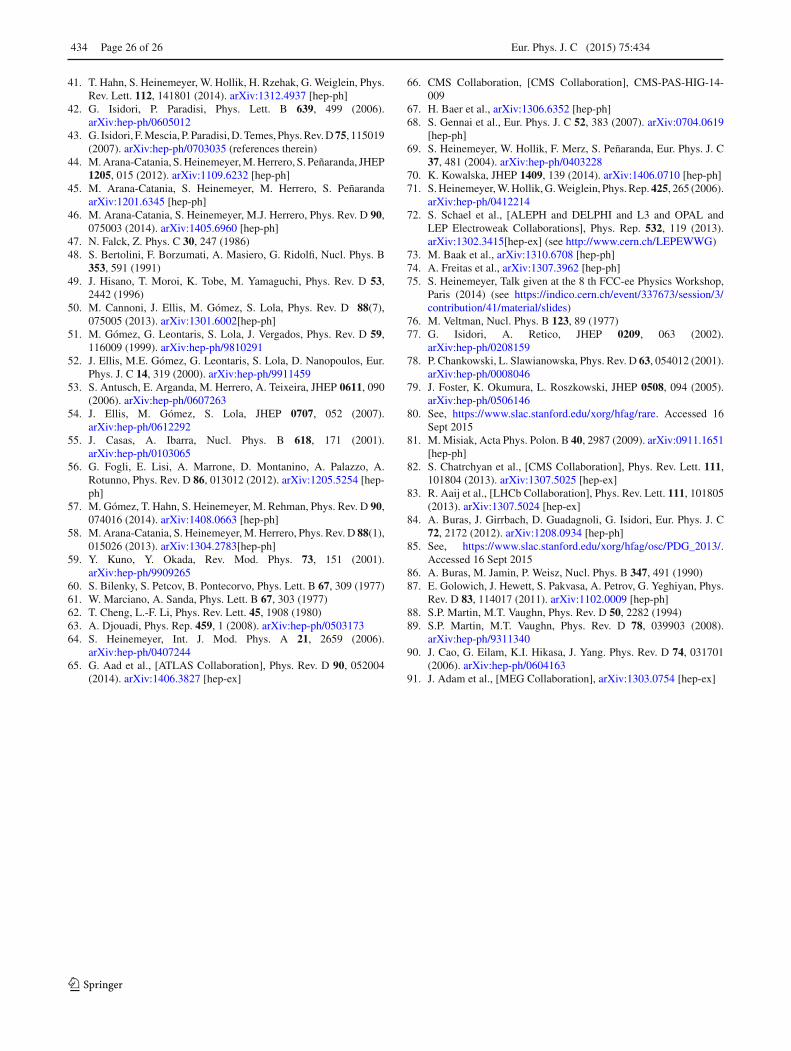
434 Page 26 of 26 Eur. Phys. J. C (2015) 75:434

41. T. Hahn, S. Heinemeyer, W. Hollik, H. Rzehak, G. Weiglein, Phys.Rev. Lett. 112, 141801 (2014). arXiv:1312.4937 [hep-ph]

42. G. Isidori, P. Paradisi, Phys. Lett. B 639, 499 (2006).arXiv:hep-ph/0605012

43. G. Isidori, F. Mescia, P. Paradisi, D. Temes, Phys. Rev. D75, 115019(2007). arXiv:hep-ph/0703035 (references therein)

44. M. Arana-Catania, S. Heinemeyer, M. Herrero, S. Peñaranda, JHEP1205, 015 (2012). arXiv:1109.6232 [hep-ph]

45. M. Arana-Catania, S. Heinemeyer, M. Herrero, S. PeñarandaarXiv:1201.6345 [hep-ph]

46. M. Arana-Catania, S. Heinemeyer, M.J. Herrero, Phys. Rev. D 90,075003 (2014). arXiv:1405.6960 [hep-ph]

47. N. Falck, Z. Phys. C 30, 247 (1986)48. S. Bertolini, F. Borzumati, A. Masiero, G. Ridolfi, Nucl. Phys. B

353, 591 (1991)49. J. Hisano, T. Moroi, K. Tobe, M. Yamaguchi, Phys. Rev. D 53,

2442 (1996)50. M. Cannoni, J. Ellis, M. Gómez, S. Lola, Phys. Rev. D 88(7),

075005 (2013). arXiv:1301.6002[hep-ph]51. M. Gómez, G. Leontaris, S. Lola, J. Vergados, Phys. Rev. D 59,

116009 (1999). arXiv:hep-ph/981029152. J. Ellis, M.E. Gómez, G. Leontaris, S. Lola, D. Nanopoulos, Eur.

Phys. J. C 14, 319 (2000). arXiv:hep-ph/991145953. S. Antusch, E. Arganda, M. Herrero, A. Teixeira, JHEP 0611, 090

(2006). arXiv:hep-ph/060726354. J. Ellis, M. Gómez, S. Lola, JHEP 0707, 052 (2007).

arXiv:hep-ph/061229255. J. Casas, A. Ibarra, Nucl. Phys. B 618, 171 (2001).

arXiv:hep-ph/010306556. G. Fogli, E. Lisi, A. Marrone, D. Montanino, A. Palazzo, A.

Rotunno, Phys. Rev. D 86, 013012 (2012). arXiv:1205.5254 [hep-ph]

57. M. Gómez, T. Hahn, S. Heinemeyer, M. Rehman, Phys. Rev. D 90,074016 (2014). arXiv:1408.0663 [hep-ph]

58. M. Arana-Catania, S. Heinemeyer, M. Herrero, Phys. Rev. D 88(1),015026 (2013). arXiv:1304.2783[hep-ph]

59. Y. Kuno, Y. Okada, Rev. Mod. Phys. 73, 151 (2001).arXiv:hep-ph/9909265

60. S. Bilenky, S. Petcov, B. Pontecorvo, Phys. Lett. B 67, 309 (1977)61. W. Marciano, A. Sanda, Phys. Lett. B 67, 303 (1977)62. T. Cheng, L.-F. Li, Phys. Rev. Lett. 45, 1908 (1980)63. A. Djouadi, Phys. Rep. 459, 1 (2008). arXiv:hep-ph/050317364. S. Heinemeyer, Int. J. Mod. Phys. A 21, 2659 (2006).

arXiv:hep-ph/040724465. G. Aad et al., [ATLAS Collaboration], Phys. Rev. D 90, 052004

(2014). arXiv:1406.3827 [hep-ex]

66. CMS Collaboration, [CMS Collaboration], CMS-PAS-HIG-14-009

67. H. Baer et al., arXiv:1306.6352 [hep-ph]68. S. Gennai et al., Eur. Phys. J. C 52, 383 (2007). arXiv:0704.0619

[hep-ph]69. S. Heinemeyer, W. Hollik, F. Merz, S. Peñaranda, Eur. Phys. J. C

37, 481 (2004). arXiv:hep-ph/040322870. K. Kowalska, JHEP 1409, 139 (2014). arXiv:1406.0710 [hep-ph]71. S. Heinemeyer, W. Hollik, G. Weiglein, Phys. Rep.425, 265 (2006).

arXiv:hep-ph/041221472. S. Schael et al., [ALEPH and DELPHI and L3 and OPAL and

LEP Electroweak Collaborations], Phys. Rep. 532, 119 (2013).arXiv:1302.3415[hep-ex] (see http://www.cern.ch/LEPEWWG)

73. M. Baak et al., arXiv:1310.6708 [hep-ph]74. A. Freitas et al., arXiv:1307.3962 [hep-ph]75. S. Heinemeyer, Talk given at the 8 th FCC-ee Physics Workshop,

Paris (2014) (see https://indico.cern.ch/event/337673/session/3/contribution/41/material/slides)

76. M. Veltman, Nucl. Phys. B 123, 89 (1977)77. G. Isidori, A. Retico, JHEP 0209, 063 (2002).

arXiv:hep-ph/020815978. P. Chankowski, L. Slawianowska, Phys. Rev. D 63, 054012 (2001).

arXiv:hep-ph/000804679. J. Foster, K. Okumura, L. Roszkowski, JHEP 0508, 094 (2005).

arXiv:hep-ph/050614680. See, https://www.slac.stanford.edu/xorg/hfag/rare. Accessed 16

Sept 201581. M. Misiak, Acta Phys. Polon. B 40, 2987 (2009). arXiv:0911.1651

[hep-ph]82. S. Chatrchyan et al., [CMS Collaboration], Phys. Rev. Lett. 111,

101804 (2013). arXiv:1307.5025 [hep-ex]83. R. Aaij et al., [LHCb Collaboration], Phys. Rev. Lett. 111, 101805

(2013). arXiv:1307.5024 [hep-ex]84. A. Buras, J. Girrbach, D. Guadagnoli, G. Isidori, Eur. Phys. J. C

72, 2172 (2012). arXiv:1208.0934 [hep-ph]85. See, https://www.slac.stanford.edu/xorg/hfag/osc/PDG_2013/.

Accessed 16 Sept 201586. A. Buras, M. Jamin, P. Weisz, Nucl. Phys. B 347, 491 (1990)87. E. Golowich, J. Hewett, S. Pakvasa, A. Petrov, G. Yeghiyan, Phys.

Rev. D 83, 114017 (2011). arXiv:1102.0009 [hep-ph]88. S.P. Martin, M.T. Vaughn, Phys. Rev. D 50, 2282 (1994)89. S.P. Martin, M.T. Vaughn, Phys. Rev. D 78, 039903 (2008).

arXiv:hep-ph/931134090. J. Cao, G. Eilam, K.I. Hikasa, J. Yang. Phys. Rev. D 74, 031701

(2006). arXiv:hep-ph/060416391. J. Adam et al., [MEG Collaboration], arXiv:1303.0754 [hep-ex]

123