.........:............'i._, _Y_ILTI: .............._77A_."7_L.._.._ :_ 77£_ ....IL.17.7.,'._,_i _: : .......Z-';;%.......• ,_,_ ,_:_ ,,_,rw_ _

___!i,_ .,:

0_'_. SEMI - ANNUAL STATUS REPORT

__ (Period Covered_ August i, 1982 - Janaary 31, 1983)

_i !.i _'k' ' •EFFECTSOF SPECIES

TURBULENT REACTING }7_OWS *

.,_ i:: _

i

" D. Goldstei_, F. Magnottl and W. Chinitz **> v;,_ .

_ %2 _- The Cooper Union Research Foundation, Inc.. New York, New York 10003

o

J

., (NASA-CR-I69767) A COI'IPIREHENSIVI[ _CDEL TO N83-16669DETE_IN_ TV,_ EFFECTS Of' T]_EFATUI;]_ AND

"_ SPECIES FLUCTUATIONS ON REACTICN _A_ES IN

_ TU_B_LEN_ _FACrING FLOWS Semiann,lal Status Ubclas

__'i:2, Report, I Auq. 1982 - 31 Jan. l_83 (Cooper 0.3/3_ 02535

o

....•-- * Work supported under Grant No. NAG1 - 18, National Aeronautics an_

•: Space Administration, Langley Research Center, High-Speed Aerodynamics

Division, Hypersonic Propulsion Branch, Hampton, VA 23665

o.o:_" • ** Principal Investigator

https://ntrs.nasa.gov/search.jsp?R=19830008398 2018-05-19T13:14:36+00:00Z

r''

" .

r._

TABLE OF CONTENTS

Page

i. Summary 1

2. Effects of Temperature and Species Fluctuations on 2

Reaction Rates in Turbulent Reacting Flows

3. An Investigation of the Ranges of Applicability of 31Chemical Kinetic Models of Hydrogen-Air Combustion

4. Flame Stabilization Studie_ Using a Pezfectly-Stirred 38Reactor Model

References 43

Nomenclature 45

Tables 47 - 52i,

Figures

d

..... SUMMARY

: The status of three tasks related to reaction rates in

i turbulent, reacting flows are reviewed. The work dealing with

: assumed - pdf modeling of reaction rates is currently investiga-

L ring a three-variable pdf employing a "most-likely pdf" model.

if"" Studies related to appropriate chemical kinetic mechanisms treat-

_.: ing hydrogen-air combustion have been initiated; their current

,-. status is reviewed. Perfectly-stirred reactor modeling of

o,_ flame-stabilizing recirculation regions was used to investigate

i L the stable flame regions for silane, hydrogen, methane and

i_ propane, and for certain mixtures thereof. It is concluded that

I - in general, silane can be counted upon to stabilize flames only

_ : when the overall fuel-air equivalence ratio is close to or

.... j greater than unity. For lean flames, silane may tend to destabilize

- the flame. Other factors favoring stable flames are high initial

"_ reactant temperature and system pressure.

-i-

b

{, :? -,.., , ............ _: ..

I

•,to•

;iv

!

•L , L,. •

•• EFFECTS OF TEMPERATURE AND SPECIES FLUCTUATIONS_:-

ON REACTION RATES IN TURBULENT, REACTING FLOWSL= •

|.-,

j " I

1

1. Introduction

1.1 Overview

The predictionof tur_lent reactingflows isa major concern of

currentcombustion research. Such modeling is required in order to enhance

the understandingof thephenomena involvedand to design and evaluatetheper-

formance of combustiondevices. A principleelementto be derived from the

modelingof these flowsis an expression for the reactionrates of the various

species involvedin any parHcular combustion process under consideration.

Currently, several approaches forthe determinationof the properHes

of turbulent,reactingflows exist.[I] Of thepresent approaches, the method of

utilizingan assumed probabilitydensityfunction(pdf)for temperature and species

concentrationsis selectedfor use in thisstudy. The motiv/ationfor selecting

thisapproach is itsrelativecomputationalsimplicityand basis inthe probabilistic

nature of turbulence.

1.2 Objective

This work examines the effectsof temperature and species concentration

fluctuationson reactionratesin turbulentreactingflows by means of the assumed

pdf approach. The followingitems are the subjectof the present study"

-3-

I. The most:likely joint pdf of reference [2] to describe effects of

temperature and species concentration fluctuations on the reaction rate.

2. The extension o[ the most-likely joint pd[ of reference [2] to three

_o _ variables. This pdf is also used to describe temperature and species concentration

_ ' fluctuations on the reaction rate.

Section..2•presentsthe general theoryof pdf'sand theiruse in calculating

_ the mean turbulent reaction rate constant. Section/, presents the results ofL '_0.

:_ . these calculations. Section 5 presents the conclusions and direction for further

" study.' :IT

o.°.

: ,.o'2

2 • -" " P " " '

°• e

-- 4 --

°.

D

r !

_°

" ORIGINAL P;0_L__:":_" OF POOR QU_L;TY 2. General Theory,

....= . 2.1 Continuous Random Variables and Probability Density Functions

:_, . A variable x may be thought of as a continuous random variable if it -

can assume all values in some interval, where the endpoints of the interval may

be plus and minus infinity. In a rigorous mathematical sense, x is said to be

. a continuous random variable if there exists a function p(x), which satisfies• the following conditions: [3]

_ pCx) -• o

• .=J pCx) dx = 1

NIt should be noted that p(x) by itself does not represent a probability,: but rather

the area under the curve from a to b represents the probability that the continuous

random variablex willhave a value somewhere on the interval. Thus the inter-

pretation of equation (lb) is that the probability that x has a value somewhere over

theentirerange of values is unity. Ifthe Ixlf is definedon a finiteclosed interval,

,: [a,b],the probabilityof x having a value outsidethisinlerva]must of course be

ze ro.

The expected, or mean value, of a continuousrandom variablex is i

definedas: [3]

Px= ECx)-==f=x p(x)dx (2)

• OF I'_:JG_,,_QUf!.LI:"_', 1

: The variance of this same variable is defined as: [31

• °x2= VCx)=._( x - ECx))2 pCx)dx (3)

_=_' " The square root of the variance is the standard deviation.

" The conceptofthemean valueofa continuousrandom variablecanbe

•i- :.. extended to functions of a continuous random variable. For example, let h(x)

be sucha function.Then, themean valueofh(x)is: [31

:!-:.... h(x)= ._f hCx)pCx)dx (,_)

.. Probabilitydensityfunctionscan be definedformore thanone continuous

- random variable.These are sometimestermedjoint,multivariableor multi-i

dimensionalpdf's.For a jointpdfoftwo continuousrandom variables,the

pt-obability is represented by the volume under the surface described by theJ

. • pdf. For Sucha pdf,p(x,y),theconditionscorrespondingtoequation(I)are: -

p(x,y) > o

(5)_ ,/'*_ f_ p(x,y)dxdy = 1

o_, -@O

_- The conceptsof"moments"ofa one-dimensionalcontinuousrandomd-

: variablemay be extendedtomulti--dimension_Icontinuousrandom variables.For_/ '

example,thejointmoment abouttheoriginofa two-dimensionalcontinuousrandom

variable,(x,y),isexpressedas: [3]

: la xy = col_.®/'xyp (x,y)dxdy (6)

-- : By comparison,equation(6)isseentobean extensionofequation(2).

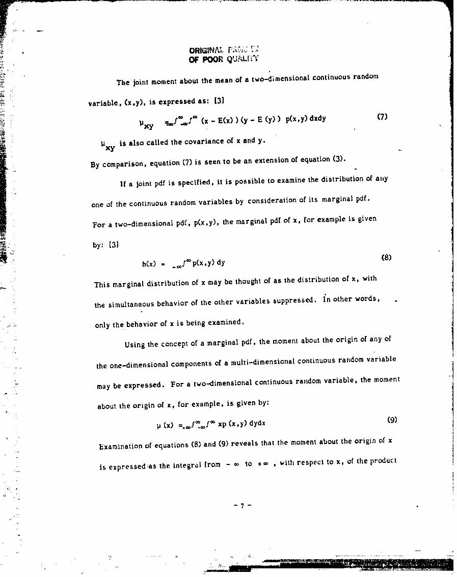
i_' OF POORQ'JALI_';'

!_._ The joint moment about the mean of a two-dimensional continuous random

... variable, (x,y), is expressed as: [31

_ _ _xy =.oj_J 'm (x E(x) ) (y - E (y)) p(x,y) dxdy (7)*

l_xy is also called the covariance of x and y.

By comparison, equation (7) is seen to be an extension of equation (3)•

If a joint pdf is specified, it is possible to examine the distribution of arty

one of the continuous random variables by consideration of its marginal pdf•

For a two-dimensional pdf, p(x,y), the marginal pdf of x, for example is given

.... h(x) = ._./'®p(x,y) dy (8)

- This marginal distribution of x may be thought of as the distribution of x, with

.. the simultaneous behavior of the other variables suppressed. In other words, .?

.... only the behavior of x is being examined.

• Using theconcept of a marginal pdf, the moment about the originof any of

:- the one-dimensional components of a multi-dimensional continuous random variable

_" may be expressed. For a two.dimensionalcontinuousrandom variable,the moment_°

about the origin of x, for example, is given by:

l_(x) =m/m f® xp (x,y)dydx (9) dl

o' ' i

,. Examination of equations(8)and (9)reveals thatthe moment about the originof x

• is expressed _asthe integralfrom - ® to +_ , _ith respectto x, of the product

.-_. •

,, _ '_ ....... r) _. _) , _,................................ _"v

_L :'

7° Op.IGtHALPP GEOF pO0_ QUALI'_f

:_ - of x and its marginal pdf.

_ . In the case of joint pdf's and functions of more than one continuous random

_.... variable, a similar expression to equation (_) can be written. For a function

dependent of two continuous random variables, say g(x,y), the mean value is

writtenas: [3]f

O0 OO

= ._f._/ g(x,y) p(x,y) dxdy (9)

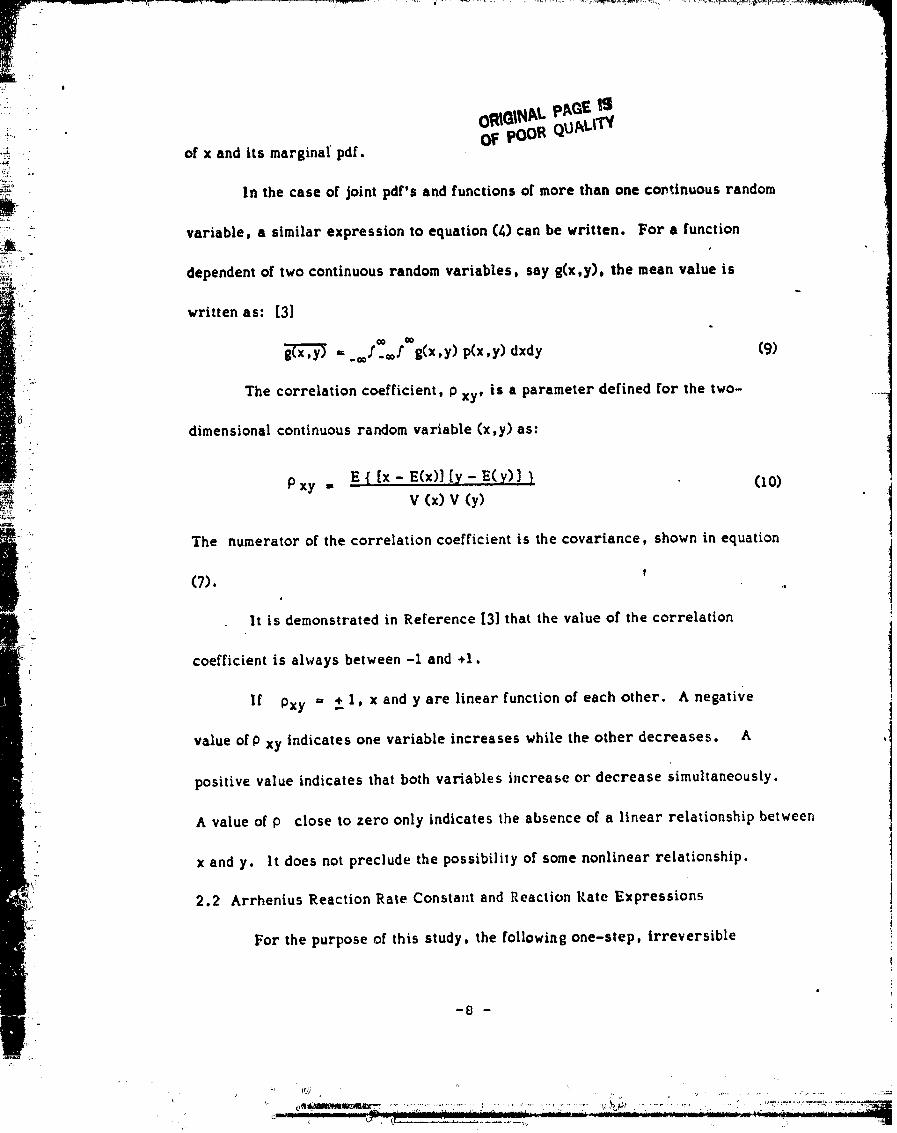
The correlationcoefficient,p xy' is a parameter defined for the two-

dimensional continuous random variable (x,y)as:• t

m m

Pxy = E{[x E(x)][yE(y)]} (z0)!_!b V (x)V (y) '|

_i' (7).Thenumerator of the correlationcoefficientis the covariance,,shown inequation,Q

It is demonstrated in Reference [3] that the value of the correlation,2

coefficientis always between -I and +I.

If Pxy -- + 1, x and y are linear function of each other. A negati','e

value of 0 xy indicatesone variableincreases while theother decreases. A

• positivevalue indicatesthatboth variablesincrease or decrease simultaneously.

A value of P close to zero only indicatesthe absence of a linearrelationshipbetween

x and y. It does not preclude the possibilityof some nonlinear relationship.t,!:_

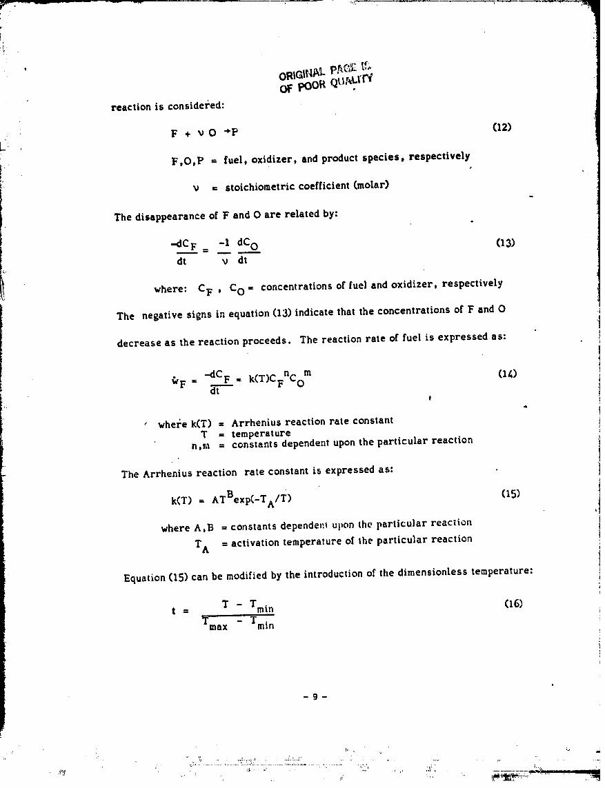
2.2 Arrhenius Reaction Rate Constant and Reaction Rate Expressions

For the purpose of thisstudy, the followingone-step, irreversible

; ,..-qP

i

reaction is considet_ed:

F + _ O "_'P (12)

Ii" F,O,P = fuel, oxidizer, and product species, respectively

= stoichiometric coefficient (molar)

The disappearance of F and O are related by:

--dCF -1 dC0 (13)

!_ dt v dt

where: C F , C O = concentrationsof fueland oxidizer, respectively

The negativesigns in equation(13)indicatethattheconcentrationsof F and O

decrease as the reactionproceeds. The reactionrate of fuelis expressed as:

"dCF = k(T)CFnCo m (I_)¢VF=t

" whe � �k(T)= Arrhenius reactionrateconstantT = temperature

n,m = constants dependent upon the particular reaction

The Arrhenius reaction rate constantisexpressed as:

4

k(T) = ATBexp(-TA/T) (151 ,'twhere A,B = constantsdependeJ:1upon the pariicu}arreaction

T A = activationtemperature of the particularreaction

4Equation(15)can be modifiedby the introductionor thedimensionless temperature:

t = T - Tmi n (16)

Tma x - Tmin

-- 9 _

i, _>"" o L .c, _. .......:......._ . :.A_...:.,

' /i. '" :.,.

OF pOORQ_jhLITY

il The temperatures Tmax and Tmi n are defined so that the dimensionless temperature

::: ! can only assume values within the interval [0,11, Thus, Tmi n may be the lowest

, temerature of the unreacted constituents and Tma x may be the equilibrium combustion

temperature of the reaction. Substitution of (16) into (15) yields:

'-. k(t)= A(klt + k2)Bexp [-TA/(klt + k2)] . (17)

o. " where k! -- Tmax -Tmi no

2'

. k2 = Tmin4.

' Equation (1_) is also modified by the introduction of the following dimensionless

concentrat ions:

....... Comin_-- rF = CF - cFmin r0 = Co - (18)

max rain comaX - Comin, ::" . CF - CF

In these expressions, "max" and "rain" denote maximum and minimum values,

respectively.Equation(18)ensuresthatrF and rO onlyassume valueswithin" i

" theinterval(0,I). For thecasewhere theminimumconcentrationsare zero;and •:

i

themaximum concentrationsare theinitialvalues,thecombinationofequations ,_

(1_) and (18) yields"

'#F = k (t)(rFC_;)n(roC_) m (19)

:- where C_, C0 = initialconcentrationsoffueland oxidizer,respectively_J

2'

..... 10 -

2.3 Mean Turbulent Arrhenius Reaction Rate Constant andMean Turbulent Reaction Rate Expression_

In a turbulent reacting flow, the mean turbulent Arrhenius reaction rate

constant can be calculated by t_'eating the temperature as a continuous random

variable and specifying an appropriate probability d_nsity function for the

temperature. This concept is employed in Reference [4], along with the

analogs of equations (4) and (17) in the present work, to yield:

_ _ = 0f I k(t)p(t)dt (20)

where _ = mean turbulentArrhenius rea:.tionrate constant

: The above expression provides a direct, relatively simple method of taking into

account the effectsof temperature fluctuationson the Arrhenius reactionrate

constantin a turbulent,reactingflow.

Sim'ilarly,the expression for the mean turbulentreactionrate can be

: developed from an extensionand combinationof equations(I0)and (19)..Thus:

w--_ =0J'10/I 0 j'l _FP(t,rF,rO) dt dr F dr O (21)

where wF = fnean turbulent reaction rate of fuel 6

This expression utilizes a joint pdf for temperature and species• Equations (20)

and (21)can be appliedto one-step mechanisms or, multi-stepmechanisms, by

consideringeach elementary reactionseparately. The pdPs used here are

considered to be validat an in_tantin time, and thus are notfunctionsof time.

-11-

} "

OF POOR QUALITY, •

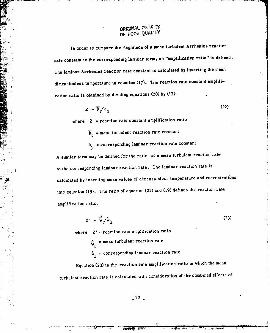
, !!i ; In order to compare the _agnitude of a mean turbulent Arrhenius reaction

rate constant to the corresponding laminar term, an "amplification ratio" is defined,

The laminar Arrhenius reaction rate constant is calculated by inserting the mean

dimensionless temperature in equation (17). The reaction rate constant amplifi-

cation ratio is obtained by dividing equations (20) by (17):

1

: Z = -_t/k 1 (22) ...._,

where Z = reaction rate constant amplification ratio '

"_t = mean turbulentreactionrate constant

_ -- corresponding laminar reaction rate constantL,

_ " A similarterm may be definedfor the ratio of a mean turbulentreaction•raze

l to the corresponding laminar reactionrate. The laminar reactionrate is= 'i,

_"_B._ calculatedby insertingmean values of dimensionlesstemperature and concentratibns

' . intoequation(19). The ratioof equation(21)and (19)definesthe reactionrate

amplification ratio:

?

. z' = _/_z (23)%

• where Z' = reactionrate amplificationratio

- -- = mean turbulentreactionrateWt

. wl = corresponding laminar reaction rate

-. Equation (23)is the reactionrate amplificationratioin which themean

•. turbulent reaction rate is calculated with consideration of the combined effects of

¢, ..

'_-........'...............-_.__..•..._"r_...............___,_,_.......,-............,!L..... : ........ - ,._

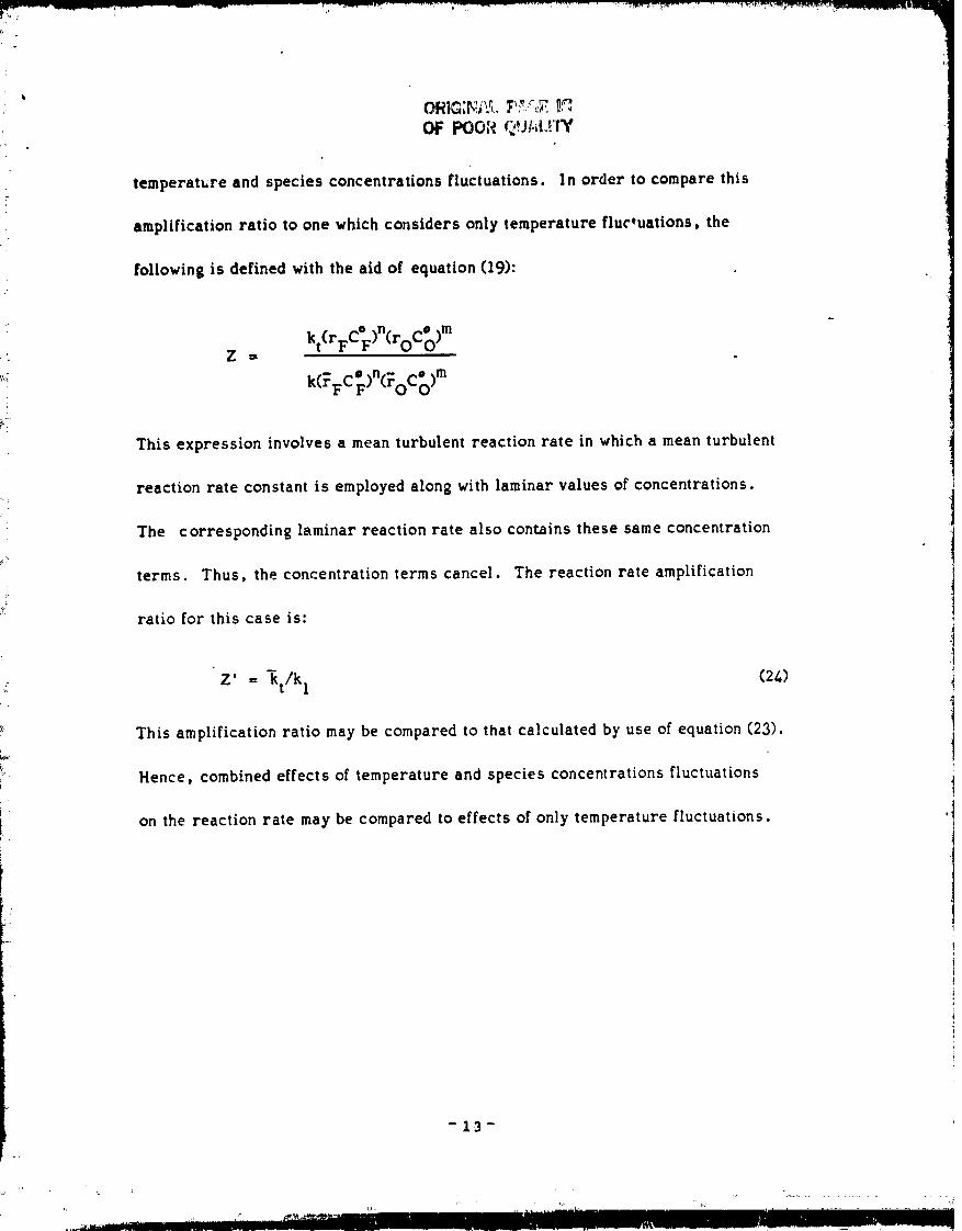
temperature and species concentrations fluctuations. In order to compare this

amplification ratio to one which considers only temperature fluctuations, the

following is defined with the aid of equation (19): ,..

on • m

kt(rFC F) (roC O)Z =

: on- om_+ k(, FC F) (roC O)

This expression involves a mean turbulent reaction rate in which a mean turbulent

reaction rate constant is employed along with laminar values of concentrations.

: The corresponding laminar reaction rate also contains these same concentration

_'terms. Thus, the concentration terms cancel. The reaction rate amplification

!

ratio for this case is:

Z' = ktlkl (24)i.

I> This amplification ratio may be compared to that calculated by use of equation (23).

! Hence, combined effects of temperature and species concentrations fluctuationsiF

on the reaction rate may be compared to effects of only temperature fluctuations.

-13-

.'r'v'_Wm==_r'_ _"_r'_-_. r'--___ _ ...... _ °_'__ _ "_"_: _"r __,'__ "r_¸¸.r'"'v,_-,,_r _

OF POOR QUALII_3/

, 3. Joint Probability Density Functions ForTemperature & Species

'i

3.1 Most-Likely Bivariate pdf for Two SpeciesI ,.

A model which accounts for the combined effects of temperature fluctuations

-_ and concentrations fluctuations of both fuel and oxidizer species, explicitly,.

ii on the mean turbulent reaction rate is presented in this section. As an initialstep inthe formulationof such a model, temperature is treatedas an independent

random variable, and as such, has no effect on the species concentrations.

Mathematically, the three-variable pdf for temperature and species is

expressed as:

p(t,rF,r O) = f(t)g(rF,rO), O< t 5 1 (25)

O_.r F & 1

O<ro< - 1

where f(t) = a pdf for temperature

g(rF,r O) = a join: pdf for the concentrations of fuel andoxidizerspecies

for the case where temperature is treatedas an independentcontinuousrandom

variable. Equation (25) is a valid pdf since it satisfies the following extension

of equations (Sa) and (5b) for a three-variable pdf:

p(t,rF,r O) .2 0 (26a)

Q_0fl ° t t p(t,rF,rO)dt dr F dr O = I (26b)J

-14 -

l' OF POOR QUALrI'Y

._ The most-likely bivariate pdf is usedas the joint pdf for the concentrations

of fuel and oxidizer species in this model. The most likely bivariate Ixlf of

-_ Reference [./4] can be written in the generalized form:,, -:°

'T_ ",

PX (_) = q (_')exp (E0- An,_n) (27) _

where q(_)isthea prioriprobabilitywhich,fornon-reactivescalars,isa

constant. The (k+l) coefficients A are uniquely determined from the

moments and from the condition that the pdf integrates to unity. When the

:_ first three moments are known for the pdf, it shows excellent agreement with

,._ experimental data.

As an initial step in the utilization of the most-likely bivariate pdf for

I

-_ two species, a pdf based on the first moment about the origin of each species :

concentration and the covariance of the two concentrations is selected. The

exp_'ession for the chosen form of the most-likely bivariate pdf for two species

iiS:

(_. -

g(rF,rO) = q • exp( _'O+ )'IrF + )'2 ro + )'3rFro) (?!:_

: where q = a constant

rF = dimensionless concentration of the fuelm _

_.: r_ ,: dimensionless concentration of oxidizeru

The continuous random variables in equation (28) are treated as passive scalars.

-15-

: OF POORQUALITY

_ With this simplification, the "q" term in equation (28) is a constant. The value

of this constant "q" term is shown in Appendix A o._ Re_.. 2 to have no effect on the

calculated value of the most-likely bivariate pdf and the values of the resulting

: reactionrates.

The values of the constant coefficeints, )'0' X l'X 2' _'3' in equation

...._,:, (28) are obtained from the simultaneous solution of the following constraint

_= equations for known values of r F, rO and r_ r_ :

_ : oJ" Qf g(rF,rO)drFdr O = I (29)

0J" 0 rF g(rF,rO)drFdr O = _F (30)

o f o r O g(r F,rO)dr F dr O = _O (31)1 !

i of of (rF-_ F) (ro-7 O) g (rF,r O) dr F dr O = r_:r_ (32)- ? ;iC"_ ',:

_." The pdf selectedfor temperature is eitherthe beta pdf, the one-variable

most-likely pdf, as presented in reference [2] or the ramp pdf, based on certain

_ "" criteria specified in Reference [5]. The development and utilization of these

: ... criteria are discussed in Reference [5] and will not be discussed here.

• Equation (25) is used in an expression for the mean turbulent reaction rate

,:" by consid_-ring the one-step, irreversible reaction, as in Section 2,2:

:- F + vO "* P

. where F,O,P = fuel,oxidizerand product specif.s,respectively

v = stoichiometriccoefficient(molar._

-16-

• , • •...... "w i*w_

• OR!$!_Y'_,. _,',':'.:V _:_OF POOR QUI_LFi_ _

,_: Assuming that both n and m are equal to unity in equation (19), the reaction rate7

•- of the fuel may be written as:

' For the case of statisticalindependence between temperatureand species

: concentration,the expression for the mean turbulentreactionrate of thefuelo

: speciesis obtainedfrom a combinationof equations(17),(21)and (25). Thiso ....

'" yields:

I (klt+k2)Bexp,. wt = -A 0$ [-TA/(klt+k 2) ] fit) d_ (35)

• o 1 1

• CFCoO$ 05 rFr Og(rF,rO) dr Fdr 0

-_. The corresponding value of the laminar reaction rate i._ determined by inserting

': the appropriate values of't, _F and _O into the combir.ation of equations (17)

r _ and (33)•This yields:o

.°.

0-.

The reaction rate amp]ification ratio is obtained by dividl ,. equation (3S) by (_),

This yields:

_ (klt+k2)Bexp" oJ"1 [-TA/(klt.k 2) ] f (t) d_

....... o.j, l oj" l rFro g(rF,rO)dr F dr O• Z' = (37)°

(k_+k2)Bexp [-TA/(k_+k2) ] _F _0

- -17-

• _._• . .. ,-

<, _ . -- .......... , ....... III I "

t_,i. _,_,-',mpm,-v,,_,=.__r,,_1,_,._,_p_,,v, T_m_.,_ _,_ _.,_ _,__I_,, '"¢__'_rw_,_:- ._ , _ _,

,_: OF PooR QUALITYa

The amplification ratio in equation (37) may be expressed as the product of a

term which accounts for the effects of temperature fluctuations, Z_ , and a term

which accounts for the effects of species concentrations fluctuations, Z r

; ,,'7- " These terms are expressed as follows:

,'-:_ ¢$ = (klt+k2)Bexp [-TA/(KI_+k2 ) ] f (t) dt

_ (kl"i'*k2)Bexp [-TA/(kl_'.k2 ) l

i J '

_- : 0fl0./"2 rFr O g(rF,r O) dr F dr O_,_...... Z_ = (38)

;F o6

Comparison of equations(38)and (22)illustratesthatZ_ is equal to Z.

• In this study, values of dimensionless mean concentrations are varied

over the range 0.0 to 1.0 , and the valuesof mean square fluctuationsof

. dimensionless concentration are varied over the range 0.0 to 0.1 • The

_-__ value of the correlation coefficient between the fuel and oxidizer is assumed to/r.....

be -0.9 [I]. The covariance can then be determined from:

|

0where p = correlationcoefficient

_,2 = mean square fluctuation

!

:: The computationalprocedure to determine Z r is described below:

• i

• ;,p/_¢,_ .,

OF POOR Qt!/_,_c',:/

1. Select values for _F' _0' _2 and _)2.

_ ..' 2. Calculate the covariance, using equation (39) and a correlationcoefficient of -0.9.

_ 3. Use Newton's Methodto solve for the constant coefficients of 'i, ° equation (28).

_'_ ;.: _. Integrate equation (38) to calculate Z'_%'. r *

ix The entries to the augmented matrix for Newton's Method and the related_! mathematicallimitationsfor the most-likelybivariatepdf will be described in the next

i status report. The data obtained from this par_.-..eterstudy are pre_ented in

il their entirety in Reference [6]. Representative results are presented inSection h.l. The results of this parameter study are being compared to

experimental data, to judge the validity of this model and the assumptions on

which it is based.

The model givenby Z = Z_ , Zr is currentlybeing examined in a

large-scalecomputer program at NASA Langley. The portionof the reaction

rate amplificationratiowhich accounts for temperature fluctuations,is

calculated from either the beta pdf or the ramp pdf. The selection criteria is

specifiedin Reference [5]. Zr , the portionof the reationrate amplification

ratiowhich accounts for the effectsof species concentrationfluctuationsis

supplied in the iorm of a subroutine for the computer program.

Subroutine FINDZ is called to find the value of the unmixedness multiplier,

Zr -- given themass fractionsof speciesAand B and the corresponding

fluctuationsof the mass fractions.

-19-

• OF POOR QUALITY

f The values of Z I are stored as elements of the matrix ABCD Forr • "

w The problem is symmetricgiven values of RA, RB, RSA, and RS , find Zr.

'ilin values for RA and P_ ; the same is true for values of RSA and RSE.

A finite number of values of Z' are stored in ABCD These correspond "r •

= ° toRA = O, .1, .2, ..._1, RSB = 0., .01, .O2, ..t.1.=

,. The givenvalues of RA, l_, RSA, and RSB are decimal figureswith

more than one significantfigure. Therefore, interpolationis necessary. This

_'::: is accomplished by findingthe 16 values of Z e which are nearest neighbors tor-=

i ,1

h thedesired value - one largerand one smaller. For each given value ofi "

f _ RA, RB, RSA, and RSB, these sixteenvaluesare added and the resultis

[ dividedby sixteen.i '_ ..L "F *o

i

f 3.2 An AlternativeThree-Variable ModelF"

A full three variable model for temperature and two species concentrations

is discussed in this section. The assumption of statistical independence between

temperature and species concentration has been dropped in lhis model. TheL ,

: assumed pdf for the fullthree-variablemodel uses a jointpdf for both the

temperature and species concentrations, and is of the form:

p(t,rF,r O) = q. exp(X0+_it+;_2rF+)_3ro+),,,tr +_stro+_,_r r ) (/,0)• F PO

where q = a priori probability !." i

_°." " )'0-_'6 ffiadjustableconstants I,

J

.. - 20 -

\\ _,_ __

f_ h _,.:_, ,, .'._,. ....

, ; OF POOR QUALfr_'6..,

,; This full three-variable model is an extension of the statistically "n, ost-

=_) _ likely" bivariate pdf in Reference [/_] as shown in equation (27), when all of

?.,, I-

LL. the first and second moments are known for the pdf. The physical justification

_( for using this pdf and extensions of it was previously discussed in Section 3.1.

_,,:, The values of the constant coefficients, _0' _1' )_2' Ik3';k X 5' and _-6'_ , _.,_..

.,. in equation (40) are obtained from the simultaneous solution of the following

-_ , constraint equatiors for know. values of _', r'F' , r_t', r 6t', rb;z'6 :

o

oj, l I• _ of of ZP(t, rF, rO) dtdrFdrO = 1 (/_1)

.... ._: o Szo$zofltp(t' rF,rO) dtdrFdr O = t (_2)

- 0fz j.z fz0 o r pCt,rF,rO) dtdrFdrO = _F (13)l l l

i ' oJ" 0J" 0J' roP(t,rF,r O) dtdrFdrO = _O (_)

--_i_ oSZoSZo$ z(t-'t)(rF- p(t,rF,rO) dtdrFdrO = _ (_5)Y

_ik. 0./"z z $ z - FO) p(t, rO) dtdrFdrO (/-,6)o[ o (t-7)(r O r F, = t'T 6

,,ii o.Vlofl j,2o (rF - _F )(rO - r'o) p (t,rF, rO) dtdrFdrO = r_r6 (/,7)

The temperature and speciesconcentrationin equation(/_0)are treated ,'I

as passive scalars. Nith this simplification, the "a priori" probability q is a

constant. The proof shown in l_ef. 2 . can be extneded to show that the q.?

- term in equation (_0) will not effect the calculated value of the pdf, p(t,rF,rO),

and therefore has no effect on the resulting reaction rate.

- -21 -

ORIGINAL P;,C.L_[3' OF POOR QUALITY

;._::i The pdf, p(t,rF,rO), is used in an expression for the mean turbulent reaction

:,_ rate by consideringany Irreverqble reactionof the form:

r;iZ

A "+ C + D ' (_;8)

where A, B = reactants species

L" C, D = product species .

Assuming that both n and m are equal to unity in equation (1,_), the reaction rate

.- of the fuelmay be writtenas:

_'F = k(t)(rFC _) (roC _) (_9)

A combinationof equations(17),(21),and (25)yieldan expression for the

mean turbulent reaction rate as:

0 o i _ l Bwt = -ACFCo_f. of oI(klt+k 2) exp(-TA/(klt+k 2) ) (50)

• rFrOP(t ,rF ,ro)dtdrFdr0

The corresponding value of the laminar reactionrate isdetermined by inserting

the appropriate,values of r'F'r-o'and _ intothe combinationof equations(I7),

and (33).This yields:

_l -A(k't+k2 )Bexp (-TA'(k't+k2)) rFCmFroCo (5_)

The reaction rate amplification ratio is obtained by dividing equation (50) by

(51), yielding:

-22 -

_r _ ...................__.....+..................................................•............_1

_t_ -nj'_

- _ OF POOR ' ' '

0$, , ,rFro (klt+k2)Bexp [_TA/(klt+k2)]p (torF,ro)dtdrFdro•" of of• nl i

¢.= (52)

r" YFFO (klT+k2)Bexp[-TA/(kIT+k2)]

.... Inthisparameterstudy,thedimensionlessmean temperatureand the

_' i_ dimensionlessmean concentrationsare variedovertherangefrom0.I to0.9. -

_ , The valuesofmean squarefluctuationsofdimensionlessconcentrationsand

!i"__ mean squarefluctuationsofdimensionlesstea,peratureare variedovertherange

from0.01to0.09. The correspondingvalueofthecovarianceforr_ r-----_

-_• isdeterminedfromequation(39)usingan assumedvalueofthecorrelation

. coefficientof-0.9(I). The covarianceforr_t+ and r-_ are alsocalculated

i. witha correlationcoefficientof-0.9fora similarformofequation(39).

The computationalprocedure to determine the values of the reaction !

1o'"

rate amplification ratio is described below:

Procedure ]

I. Select values for T, _ F, _O,V, -'-'_rO , t'_ i- i

2 Calculate the three covariances using equation (39) and a value of

• the correlat ion coefficient of -0.9. 'i

- 3. Use Newton's Method to solve for the constant coefficients ofequation (40).

,': 4. Choose valuesforB, TA, TMIN,. TMA X.

_i 5. Numericallyintegrateequation(52)tocalculateZ .

@

The valueschosenforA, B, TA, TMI N, TMA X, C_, CO are giveninTable i.

.. Selected results of the parameter study undertaken are

presented in the next section.

. -23 -

OF PO0t_ QUALITY

4. Results

_, : h,! Selected Results of the Most-Likely Bivariate Pdf For Two Species

_. : Allnumericalintegrationsare performedwiththeuseofSimpson's.

Rule. The number ofsubintervalson theintegrationintervalc_f[0,1]are large

i enough so that no truncation error is incurred. The resulting value of Zr-

. is accurate to five places.7-_ ° " :

In addition to the limitations of the program from Newton's Method,

F_ i" convergence problems were found from three other causes:

• 1. The value of ( )`2 + )'3 t) was a term close to zero in the denominator.

°: -" 2. The value of the pdf became greater than 1 x 1038, or less than

":" 1 _ 1(538 . This can be caused from a poor initial guess, orextreme values of the parameters.

: 3. The last problem was from one of the constraint equations. Equation.... , (32)can re rewrittenas:

=_ 0f:0.fIrFrOp(rF,rO) drFdrO = r_r_) + _F_O (53)

Sincer_r(_isalwaysa negativeterm,forcertainvaluesoftheparameterso _'j

" therighthand sideislessthanzero. Thisviolatesstatisticaltheoryand

- hence no convergence is possible for these values.

" • 0

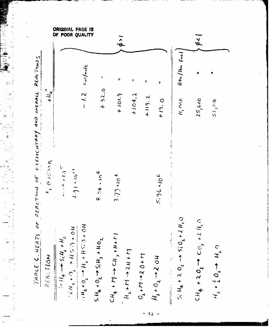
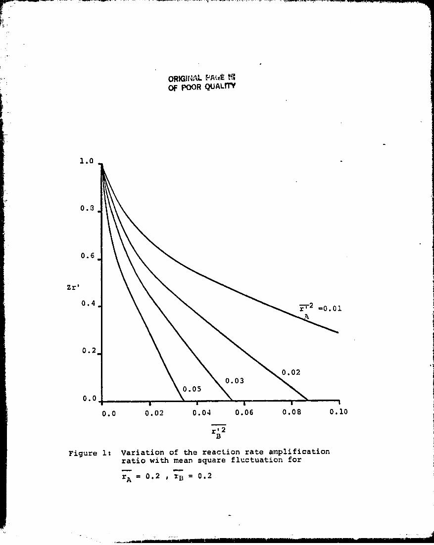
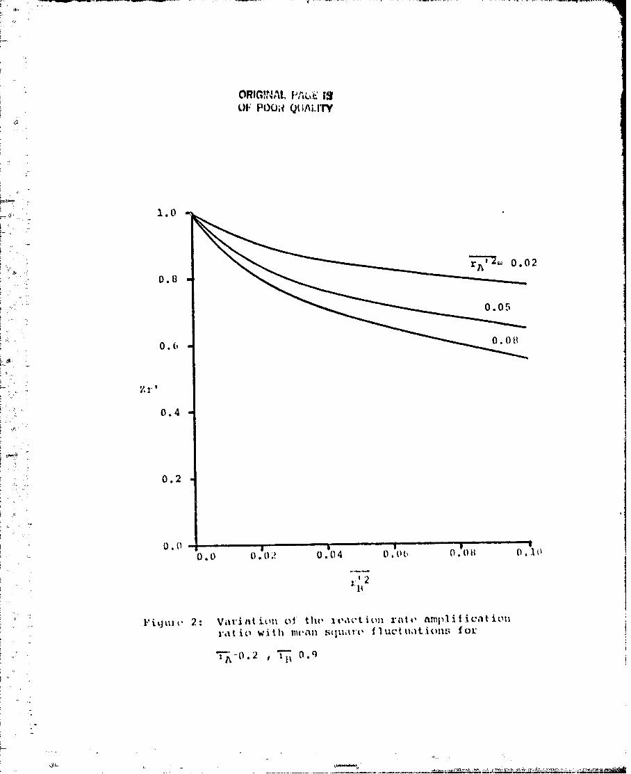
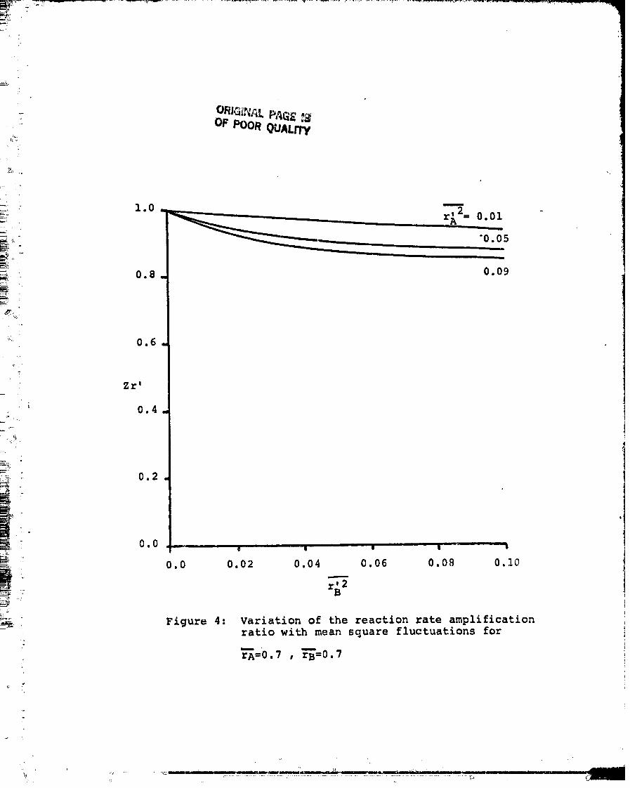
. Figures I - _ show the variation of Zr with increasing mean square. ,q

_:' fluctuations at constant mean species concentrations. As the fluctuations increase,

Zr' always decreases. The lower limit ofZ r' is zero, the case where there is

_: no reaction. This will occur when the turbulence is So great that the fluctuations

-24 -

......... II,,, I I lllli ' 7" _' [" " lr[l [ II( i" 'II" I I

_i '_ _¸ _'"_"_'_"_ '_"_'.m -- _,,'-_',_,'_m _--¸ , - . -'._'-+_ .

OF PO0f_ QU;_LI'TC

_ inhibit the reaction, or where one of the species is not present.

- Because of the convergence problems indicated with the computer program,

° i results for values of the fluctuations were linearly extrapolated.

high mean square

_!: _.Once a value of zero was reached, it remained zero for all higher values of mean

square fluctuations. For the upper values of mean species concentrations Zr'

is approximatelyconstantand approaches a valueof 1.0.

_! Figure 5 shows the variation of Zr' vs mean species concentration for

constant values of mean square fluctuations. The value of Zr' increases with

increasing mean species concentration.

_.2 Preliminary Results for the Full Three-Variable Model

To decrease the computer time to calculate each Z value for the full

three-variable model, an exact transformation was used. The triple integrals,

which must be calculated to use Newton's Method for non-linear systems, where

reduced to double integrals where the variables are separable. All of the double

integrals have the following form:

N -(k/_)o 2d o dT (54)J" f(T) ,/" o e

T o=f (T)

where N = 0, 1, 2, 3, _

The augmented matrix for Newton's Method and a sample derivation of a double 4]{

, -25 -

!:

I

: ORIGL_DJ.. l" ,_._,..'_3i OF POOR QUALITYi"

•" integral will he in n future progress report. When N _ O, the integral overr

o is a scaledVersion of the bellshaped curve. For N _ l, 2, 3, or/_,

the inte_Iral over a is a function of a and the bell shaped curve.

L !

i One of the mathematical difficulties of Newton's Method is that convergencei;

of this method is dependent on an initial guess within acceptable bounds of the

': exact answel" o

As a first s_ep toward an initial guess subroutine, restrictions were

_:: placed on the variables to reduce the full three-variable model to the two-variable

model. (Note: in the following discussioh, t is dimensionless temperature

and r and x are dinw..',ionle:,s mean specics concenlrations A and B).

• f

- ...., "lhc re.,,triction.,, on thc thv'ee-variable model are't _- r and{'2 _,2.

: t and r can be considered tttlllllny variable,; since they are irltegrated ovt, r the

same limit:,. Therefore let ! r :. y. Thv pdl can now be wriltc,n a._:

. pdf _. exp(] _0 + _I y 4_ /,y2) ,

• .exr,(l),0 ' + )'3x l),5+X :ilyx) (.','.0

" Thi.,, now gives a valut, for the pdf which cal_ bc evalt|ated [rolu the on,, and Iwo-

: variablepdf's. 'lheinitialgtles_subroutlllccan lw devclolwd by usingpower

- set'if.',around exa¢l solt|tioll,_,

"_ In the model where ] - Z i I r, t is not a funcliOll of either I- or x (',,lwci_,:,

'.'_ A or" it). Therefore. the integral over I can be placed inside thedouble integv'at

_5

_,,,,, , , , ' - _- -, = y-. " ---.:_a._,,_'t,_' _.,z_- ---_

, - _ ---_r.-.-T_m-..e _ -:=_\-.--._-. • _;_1_mvam1[_l I

= OF POOR QUAUTt'

• over r and x and Z can be calculated from:

z_°:l l zo,1" ol Q expO_ + ), +X_ t 2)

.... .exp_ + ;_t +_,_x+,_ _rx) dxdrdt (56)

. whereQ - rxexp[ -10116 ] (klt +k2)B .Klt+K 2

_! Z for the full three variable model under the restrictions indicated for

! - equation (55) can be calculated from:

I, x _ y21Z = of o J"exp[½ XO*x 1 y + X4{

, ,exp [½p, 0 + )'2 y �}'3x + (;k 5 + )' 6) yx ] dydx (57) i

Comparison of the Z value for the three variable model and Z calculated

by multiplying the one-variable temperature only pdf by the two-variable bivariate

pdf for two species can be evaluated by taking the difference between the values

and determine if it can be made arbitrarily small. In equation form:

x z _e p'O + Xlt + _2r+x3 x+,_ 4tr +P,5 tx + P6_'xZ - ZtZ r =oJ'oJ'oj" '

(581

Under the restrictions of_" = _ and_ '2 = _,2 the difference between

the Z values is exactly zero, if the correlation coefficients are as follows:

Ptr = +I.0

Otx = -0.9

Prx = -0.9

-27-

i •

There are no restrictions placed on species concentration B (_,_,2).

.}

_v

?,

OF POORQUALITY

5. Conclusions and Directionfor Future Work

5.1 Conclusions

5.1.1 Effectsof Species Fluctuationson the ReactionRate

• The effectsof speciesconcentrationfluctuationson the reactionrateare

assessed by treatingthe speciesconcentrationsas continuousrandom variables.

A joint pdf is used to relate the variables. The total amplification ratio is the

:_ mean turbulent reaction rate divided by the corresponding laminar value. The

.- reaction rate amplification ratio, which only accounts for the effects of species

°: concentrations,isdiscussed here. The resultsobtainedfor a parameter studyi-

on Z_" are the following:

1. The value of Z_" is between 0 and 1.0.

i.

: 2. For constant values of mean species concentrations of A and B .

i _: (_A' _B ) and for constant fluctuations of species A (_2), Z_"

" always decreases as fluctvations of species B(_ 2) increases.!

3. For constant values of fluctuations for species A and B and for

_._ constantmean speciesconcentrationof A, Zr increases as rAo increases.

,..

- 5.2 Direction for Future Work

I. Having exact answers to the three variable model, evaluate theerror in the program and write an inilial guess subroutine.

- 2. See how Z compares to Zt _ Zr for allof the mean quantities, not equal.o,

'." - 29 -

CP

-q

._

_ 3. Compare Z vs Z t" Zr for different correlation coefficients. One ..

• suggestion is to set the value of the correlation coefficient betweenspecies equal to -0.9 and between temperature and species equal to-0.99. These values were suggested by Anlaki [I].

a

!-

-30-

i •

i

i....

i ,

AN INVESTIGATION OF THE RANGES OF

i'ff.;,_ APPLICABILITY OF CHEMICAL KINETIC MODELS

_ OF HYDROGEN-AIR COMBUSTION

:

.°

i°

- 31 -

°

.°

_ OF POOR QUAY.I'FY

sufficient to de:l with the "combustion" process.

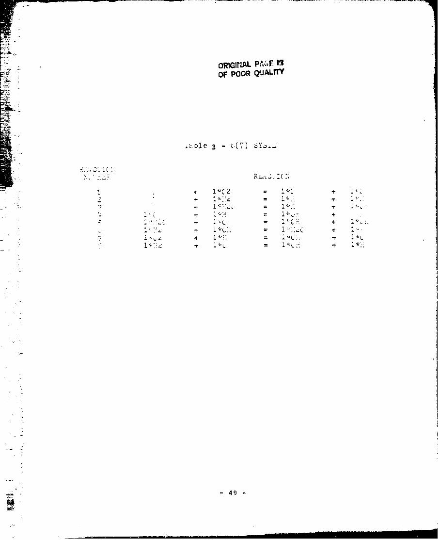
An 8(7) system ('fable 3) will be tested to confirm %he

results of Evans and Sc!_exnsyder, In oraer %o further reauce

compu_-_+,i-:':l ti_e, _ Z(4) _lobal mod_:l {'.:ule 4) developeo by

i Chinit? and Ro .-_. (hef. ll) will be tested. Las ¨ @�ˆ_:-Ter

will try to test the p_,r%i-_l equilibrium assumption (Ref. 12)

• on The zoeve systems in an effort to aosolutely mini-,ize co_pu-

T=%ion_l _i._:e. ,o acco_llsh this, a large number of one-dime.n-t

_ s_on-:l cons%ant pressure, H_ - air computations will be perforzec

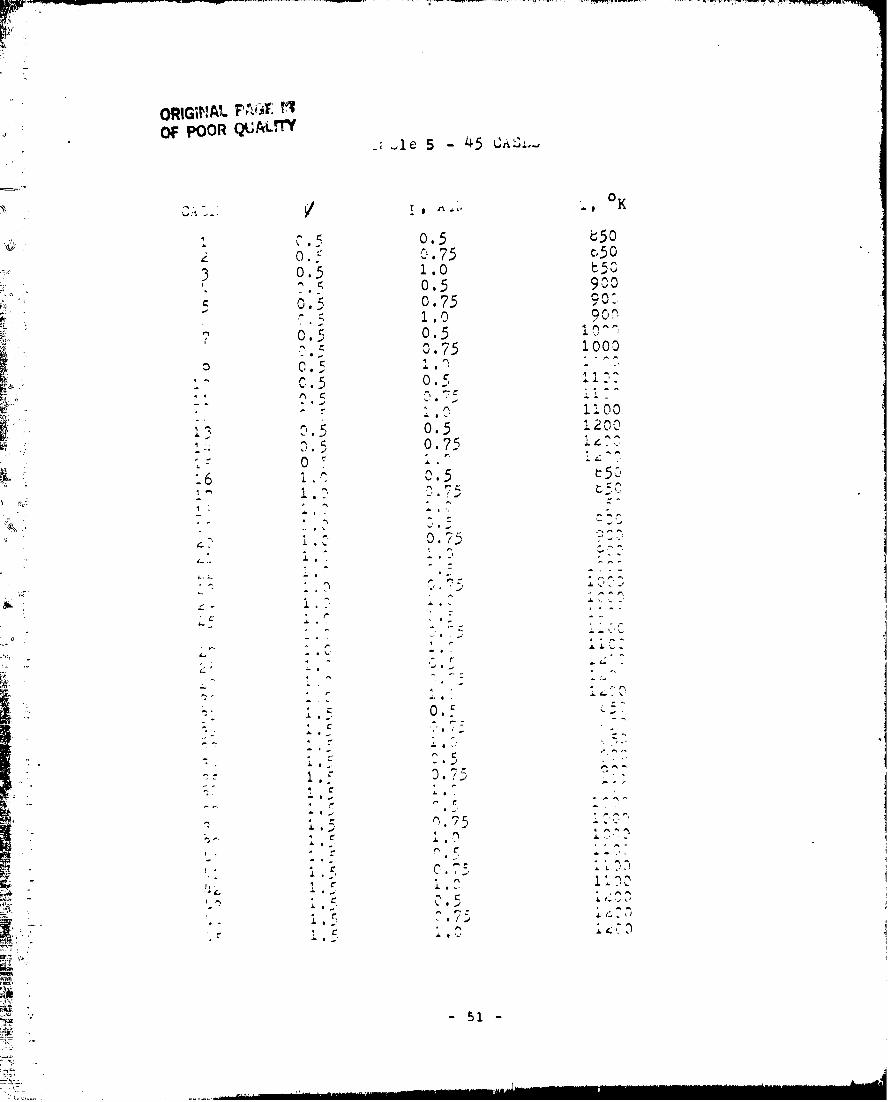
il_ _ in the r_-nge:! i-

= • 0.5 6 4 1.5

_50 4 _ z_ izOO

i _ 0.5 4 _ _L !,C[

.... ',,,here/ _s _:e -__;.ivu!ence r-_%io, I the temperature "_, o

' _ _, _ treasure in _osrhe1"es. :. list of _,:ese inaiviuu_! c_se_

_c ..-iven _n %able 5.

_lo_,,scf %he m,._lefranc%ion of %he _ri[[er s_6cie_ vers'_

'-° : _,r..t'_qn_-,; " Time _nd i_r:i%ion lime versus ignilion %e_-cer_ture "_.ii_

- i,c -_a _ccord_nce v:i_h the process aescribed _n reference 9.

7

j.

....... 34-

i .... ]:: ......L';

" OF POOR QUALITYTrel i-,inary hesults

.I

The major proL,le::,in the first semezter of work h_,a;'+

been in the ower_-tion of the computer program. '.heprogram

o had been runnin_ smoothly on the N. Y. b. operating system

un_i_ tI'e oystem, was switchea %0 a Cx__R. At present the

..._. r_<, r_ is not working out will be ol,erating wi_hb, the

n_:.a :. --.-,)._.As _ result progress has been slo,'..

:,:,. ;'. -e first 35 of the a5 cases nave oeen run usir.._--_he

1 __ extens,,'ve37(1.3) Feckage, Ca,_es io-2! using this _ack_-ge

•! _ : were termin'-.teda'ae to excessive computer running ti_:e-.

: .his Trebler h_s been encounterea before in other s_ucies.

• Fifteen c_e._ have Oeer, rut.usir:_ _ne 5(7) fro- ic:,iticn

" io _a_'l'"._riu_ _ifure_ _-12shov' the c(?) s2,;sle_co_-reu to

the ?-<13' s_'s+ '_ ., _e... 6% _ t.rez:sure cf one atmosFhere , _n equiv,.[

, fence r-rio cf 0.5, ar.u various %eml:eratures. .nic sol cf

ce-r'-r'_or:z is _3"1ic__ o tie res:ul%s founa in co._F:-rir,;%;,:£

. ="=%e." "_,i'_h. _r.e . ,. : 3) _"'-• ,,._ =o.=,%er.: r e Entire Froce<:=

;: " _nd oO0°?; the _(7) s3's;e.".,legs oet.ina the 37(13, sya_-.

....." r_r. :_-,.-,-er'.ture_ of iO_O°iL, 11090,4, and l_O0°n the 77(_" '

.... _"_e- i..-.'_oehinc t?.e _(7) system.. 'sherefore, oetv,een c'? '?'

end 19_._°;: _ transition t'=-kespl_ce, As a result %here i_ _

te-._er::.ture range a't aFFroxir,,ately 950°b; where the r(7) s:,'zte:-

demerit.or both the ignition ana combustion _rocesses.

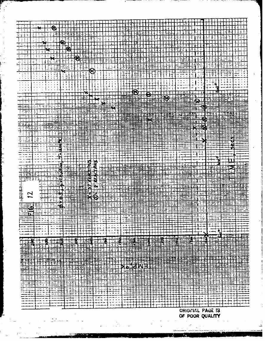
Fi-'urel3 shov'-zthe comparison of the 37(i3) an_ the

"f c) _,,_:er-_ in %he co_'uas%ion r..oae, As shov,n by _vans anu

._c_r,xn ";i_er the {,(7) _5'_te_. uescrioez the combustion Trocer:,'L

<., "nre rune of the b(?) s,vstem,startin_ at the oo_..uustion Fei',_

- 35 -

6f 1he 37(13) s.vzter are neeuea for further verifica%ion.

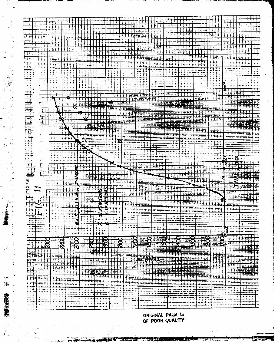
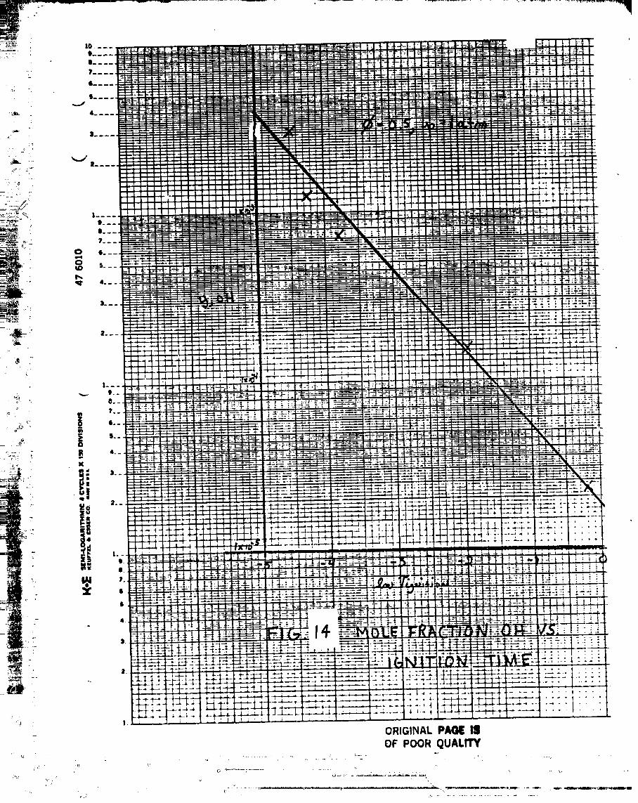
Figure14 shows n loEari_hmic _io% of mole fraction of

C.[_versus irniYion time. As shown in reference 9 the plot

_- i_ line_.r _nd is thereby, a gooa _ri_ger species. _.'.orere&%

cases will be needea to verify this.

Figure 15 shows a semilo£ari_h_..ic plo_ cf i_ni_ior,

•_ _i_ versu_ the reciprocal of iniZial temperature for

both the 6(7) _nd 97(!3) s_,stems. _he results here confir-

The work of Ro?ers end Schexnayaer.

ORIG}NAL ''_ =" _

OF PC:DR QVALITY

- 36-

........... -'_--;,_ii_,'_c L._.'_____ __t__'-___._...... _ ................... . .....

Conclusions ann Ouserv_%ions

• ',here _re preliminary conclusions basea only on _he

- ini_i_l work done so far:

< i ihe _!(7) '_* "• . s._=_e..,does not describe lhe enlire Droces_

, ;- (i.e. i_ni:ion and combustion) excep% a% 950°h, one

" _o_here, ._.naan equivalence ra_.io of C.5.r

° ;. 2. _he b(_) sysle_ aescribes zhe comous%ion _roces_-.

%. At one _mos_here _nd an equivalence raZio of 0.5

*_- lo_:._rith_-ic plot of mole frac"_ion of OF versu_= - _.. t': "";

.. irn5%ion %'_'a..: is linear.

,. .%_ %he sa-.e conaitions -_- aoove, %he effec% of inizi: 1

_e-pera_ure on irnlzion %i_e for %he 37(i}) p;-c_-ce

.. confir:"z %he re_.s.l_.-zof reference B.

O

+°

.!O.

!

_°_

, • °

i

i,_•_-

"-.

i _ FLAME STABILIZATION STUDIES USING A

i PERFECTLY-STIRRED REACTOR MODEL

J

: i

_° .

- 38-

: ORIgiNS, PAGE II

oF

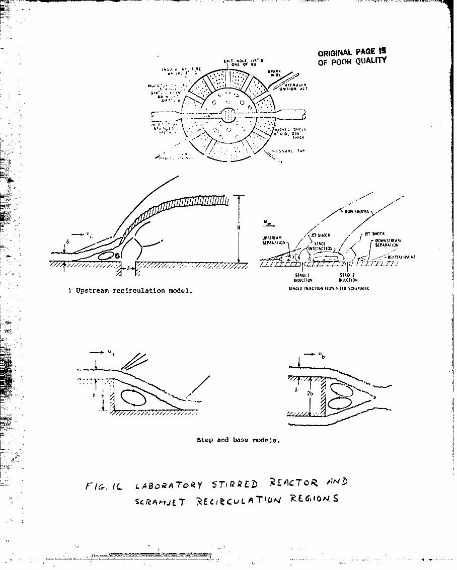
The use of the stirred reactor concept to model combustion

regions of intense mixing and recirculatlon dates to Longwell,

_ et. al. (Refs. 12 and 13). Longwell's laboratory stirred

reactor, along with regions in a SCRAMJET engine which may be

modeled using stirred reactor theory, is shown in Fig. 16.

Reactors in which reactants and inerts exist in the gas phase

only are termed "perfectly stirred"; multi-phase systems are

"well-stlrred."

A version of the perfectly-stirred reactor code developed

by Pratt (Ref. 14) was used along with chemical kinetic mechanisms

developed at LRC for ihydrogen, hydrocarbon and silane combustion

(e.g. Refs 8, 15, and 16) to investigate blowout limlts for neat

fuels and for mixtures of these fuels. Results are shown in

Figs. 17 through 27. The blowout limit, in all cases, was deter-

mined by examining computed curves of reactor temperature as a

function of the mas_ flow rate per unit reactor volume, _n/V. The

blowout llm_t was then determined as suggested in the sketch below:

T

Equilibrium Flame

J Temperature .Ia Blowout

Specified Reactants,Znitial Temperature,System Pressure, andFuel-air Equivalence Ratio

' _/v '- 39 -

:,! ,i OGIGINAL.PAGEI_OF POOR QUALITY

:. The residence time in the reactor, related to i=n/V by

._ t R - pl (_IV)

is simultaneously calculated in the computer code (Note that a;; °

.C':} recent criterion for blowout developed by R. C. Rogers was not

_* available at the time the calculations reported upon herein were

_.. made.)

-_-?_,_ Fig. 17 illustrates the effect of initial reactant temperature

:i and quantity of silane in the fuel on minimum residence times_+_i _7 required to avoid blowout of the flame• These results are for

_ _ H2 and CH 4 as the principal fuel constituents. It is of interest

that increasing Sill4 in the fuel results in a more substantial

:, + effect for H 2 than for CH 4. On the other hand, the results for II2

suggest th, a.t, at high initial temperatures, little stabilizing

. effect is achieved for H2/Si}l4 until the silane concentration exceeds+

. 5% by volume. Increasing the initial temperature, as expected,

increases the stable flame region. These same results may be noted 1

+• by reference to the cross-plot in Fig. 18.

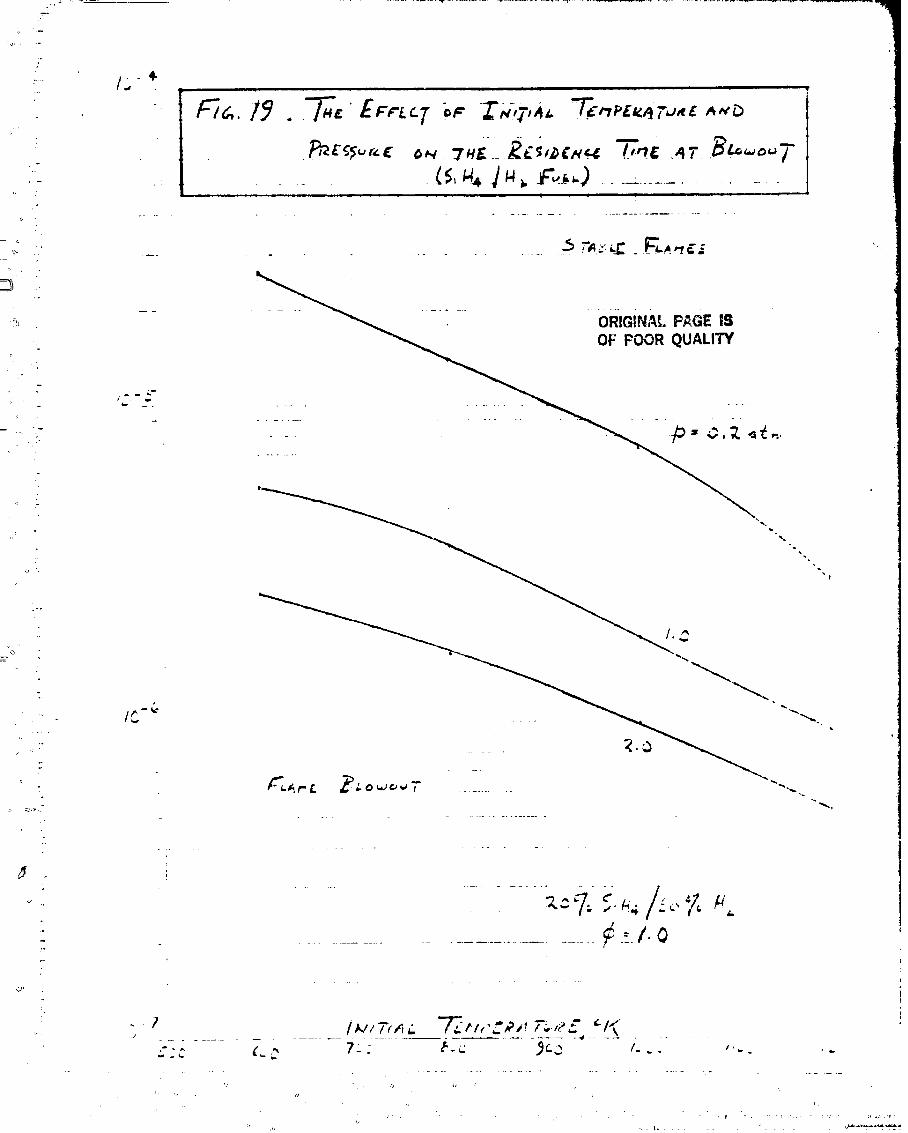
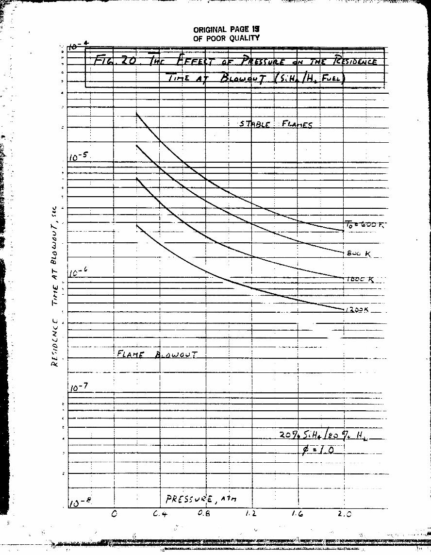
_?:_ • Figs 19 and 20 illustrate the flame stabilizing effect of_, •

_/ increasing the system pressure. As can be seen, the effect is sub-

stantial going from 0.2 arm to 2.0 atm wherein, at 1000°K for

example, minimum required residence time decreases from about 7 _,sec 1

_:* (at 0.2 atm) to about 1 psec (at 2 0 atm)

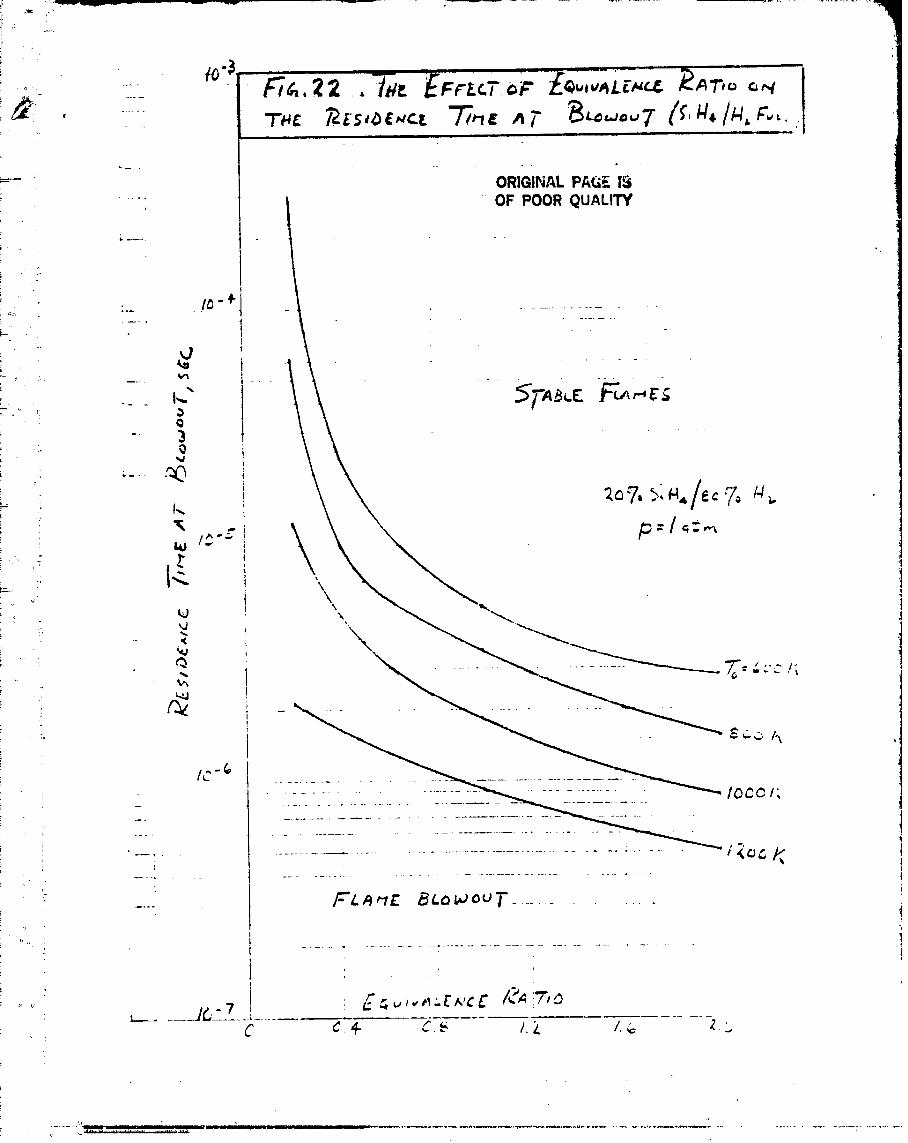
The effect of equivalence ratio is indicated In Flqs. 21 and '_'_i "

__ i for a 20% SiH4/80% H 2 fuel (by volume) at 1.0 arm. The stabiliz_nq

effect of Increasing the equivalence ratio _ is seen to be predomi-

• nant at the lower values of initial reactant temperature T For/ O"

example, at T = 600eK, t decreases from about 3 x i0 -4 see (¢ = 0.2)O R

- 40 -

J

%.

i'"' to about 3 x 10-6 sec (% = 2.0)_ a decrease of two orders-of-i

_ - magnituae. On the other hand, at TO - 1200°K, the decrease in

t R is from about 2 _sec (_ = 0.2) to 0.5 _sec (_ - 2.0}.__':_ The tradltional stirre_ reactor plot of _ versus in/V is

shown for SiH4/H 2 fuels (TO 600°K ,= , p = 1 arm) in Fig. 23. The

.&,_!... stabilizing effect of increased silane concentrations is again

_;4_; noted. Of particular interest are the following:

_# 1 The locus of maximum _n/V values increases from _ = 1 for

pure H 2 to about _ = 2.5 for pure SiH4; and

_ 2. A reversal occurs below _ = 1.0 wherein the stable flame

i_,_:_: region is greater in extent for lesser quantities of silane in the

fuel.

_ A possible explanation for these two findings is suggested in

._ . Table 6 where it is noted that the principal initiating reactions

,:_ for silane oxidation are SiH 4 pyrolysis followed by the very rapid_ ,

oxidation of the pyrolysis produce SiH 2. As seen, these two steps

t_ _ : are exothermlc. However, the direct step 02 oxidation of SiH 4 to

_. SiH 3 and HO 2 is mildly endothermic when compared with the highly

" endothermic steps which initiate the CH 4 and H 2 oxidation chains•

Hence, high silane concentrations relative to oxygen (i.e., high ¢

values) tend to result in greater flame stability due to the

exothermicity and relative rapidity of the principal chain-initiating

steps•

On the other hand, below _ = 1 flame stability is favored by

" the higher exothermicity of the overall reaction (Table 6, _<i).!

Since the heat of combustion of silane is substantially below that

of hydrogen and even the hydrocarbons, at low equivalence ratios

increased silane concentrations appear to have a destabilizing effect•

- 41 -

i, ,J

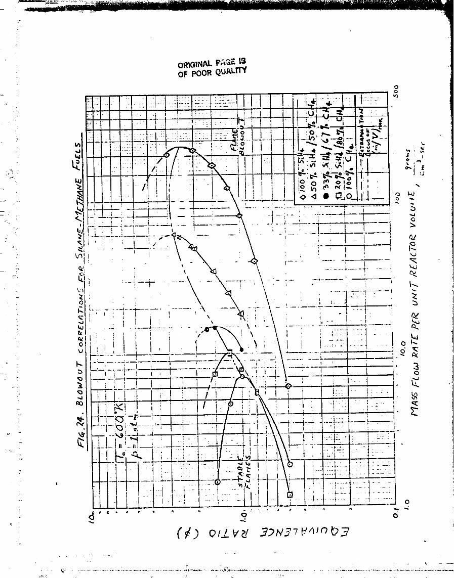
= A similar result is seen in Fig. 24 where SiH4/CH 4 blowout limits

are shown. Fig. 25 again suggests the picture detailed above. For

ii • example, the activation energy of the reaction

I _. CH 4 + M * CH 3 + H + M

}_! is given in Ref._& as about 85,755 Kcal/gmole, while for

it is given as 64,968 Kcal/gmole. Hence, the relative rapidity of

the latter tends to favor C3H 8 at _>i. On the other hand, the

higher heat of combustion of methane favors it at _<1. These

predicted trends are verified in Fig. 25.

Figs. 26 and 27 summarize the results obtained for the neat

fuels in terms of _esidence time (Fig. 26) and _n/V (Fig. 27). In

general, for _>I flame stabilization is favored by the use of

silane in the fuel mixture and by the use of the higher hydrocarbons

(above CH4). For ¢<1, silane may serve to reduce flame stability

" and the use of methane is favored over the higher hydrocarbons. Also

favoring flame stability are high initial reactant temperatures and

: high pressures.

!

F ° tl

• " REFERENCES

.... i. Antaki, P. J., "The Effects of Temperature and Species Fluctuations on

Reaction Rates in Turbulent Reacting Flows." M. E. Thesis, The Cooper

Union, School of Englnee_ing, April 1981.

_ :: 2 Foy, E., "The Effects of Temperature and Species Fluctuation on Reactiono ..

I _ _ Rates in Turbulent Reacting Flows." M.F. Thesis, The Cooper Union,School of Enoineering, April 1982.

I

[ _: . 3. Meyer, P.D., Introductory Probabilit_ and Statistical Applications,

L: - Second Edition, Addison-Wesley _ublishing Co., Reading, MA, 1972.

_. 4. Pope, S. B., "A Rational Method of Determining Probability Distributions

o ,,_ on Reaction Rates in Turbulent Reacting Flows," J. Non-Equilib. Thermo.,

V.4, 1979, pp. 309-320.

_i_.' 5. Ronan, G., "Selection Process Between Probability Density Functions that

I i' Model the Temperature Fluctuations in Turbulent Reacting Flows,"! ..... M.E. Thesis, The Cooper Union, School of Engineering, April 1982.F L.

I 7"

I 6. Goldstein, D., "Effects of Temperature and Species Fluctuations on

i .:_ Reaction Rates in Turbulent Reacting Flows," Special Report, The Cooper

_,_ Union, School of Engineering, April 1982.

7. McLain, Allen G. and Rao, C.S.R., "A Hybrid Computer Program for

Rapidly Solving Flowing or Static Chemical Kinetic Problems Involving

.,- Many Chemical Species", NASA TM X-3403, July 1976.

jl8. Rogers, R. C. and Schexnayder, C.M. Jr., "Chemical Kinetic Analysis of

Hydrogen-Air Ignition and Reaction Times", NASA Technical Paper 1856,

: July 1981.o

9. Chinitz, W., "Simplifying Chemical Kinetic Analyses of Reacting Flows

_ -. Using an Ignitlon-Combustion Model".

• i0. Evans, J. S. and Schexnayder, C.J. Jr., "Critical Influence of Finite

Rate Chemistry and Unmixedness on Ignition and Combustion of Supersonic

" H2-Air Streams", AIAA Paper #79-0355, Jan. 1979.

ii. Rogers, R. C. and Chinitz, W., "On the Use of a Global Hydrogen-Air

Combustion Model in the Calculation of Turbulent Reacting Flows",

.... AIAA Paper #82-0112, Jan. 1982.

" 12. Longwell, J. P.! Frost, E. E. and Weiss, M.A., "Flame Stability in Bluff"i

. Body Recirculation Zones", I. and E. Chem., 45, 8, Aug. 1953.

13. Longwell, J. P. and Weiss, M.A., "High Temperature Reaction Rates in

• Hydrocarbon Combustion," I. and E. Chem, 47, 8, Aug. 1955.

14. Pratt, D. T., "PSR - A Computer Program for Calculation of Steady Flow,

. Homogeneous CombustlonReaction Kinetics", Bulletin 336, Wash. State Univ.,1974.

,D- 43 -o

L

15. McLain, A. G. and Jachimowski, C. J., "Chemical Kinetic Modeling

of Propane Oxidation Behind Shock Waves", NASA TN D-8501, July 1977.

° 16. Jachimowski, C. J. and Wilson, C. H., "Chemical Kinetic Models for

Combustion of Hydrocarbons and Formation of Nitric Oxide," NASA TP 1794," Dec. 1980.

,4 ,_ , :°

;.'-_.N._ '

a

- 44 -

t

ORIGINAL PA_3E13B

oF POORqO/_LITY- ._ Nomenclatu=e

• A pre-exponential constant

" B temperature exponent '

• C instantaneous concentration _

_ C° initial concentration

....! E(x) expected(mean} value of x

F denotes a fuel species

_ f(x, y) joint probability density function of (x, y}.

_: g(x, y} function of the two-dimensional continuous random ,_"" variable (x, y) I_ g(x, y) mean value of g{x, y)

h(x) function of the continuous random variable, x

k Arrhenius reaction rate constant

• k I , k 2 constants dependent upon Tmi n and Tma x

-_ k I laminar Arrhenius reaction rate constant

q mean turbulent Arrhenius reaction rate constant

m constant, defined in equation (30) ' :

..... max denotes maximum value,i

min denotes minimum value

2 n order of reaction constant

O denotes oxidizer species

P denotes a product speciesi

p(x) probability density function of x

p(x, y) joint probability density function of (x, y)

r dimensionless concentration and constant defined

( by equation (30)

" 45-

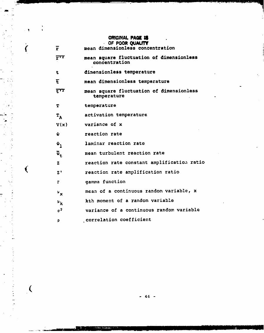
"_ ORIGINAL PAGE

_ OF POOR QUALITYi _ _ mean dimensionless concentration

r-'rT mean square fluctuation of dimensionlessconcentration

t dimenslonless temperature

_i" t mean dimensionless temperature

; _ mean square fluctuation of dimensionlesstemperature .

T temperature

:: TA activation temperature°_

- : V(X) variance of x

..... : _ reaction rate

_i laminar reaction rate

w t mean turbulent reaction rate

Z reaction rate constant amplification ratio

Z' reaction rate amplification ratio

'_ F gamma function

': _x mean of a continuous random variable, x

kth moment of a random variable

• o2 variance of a continuous random variable

, p ,correlation coefficient

•T

"" (

- 46 -

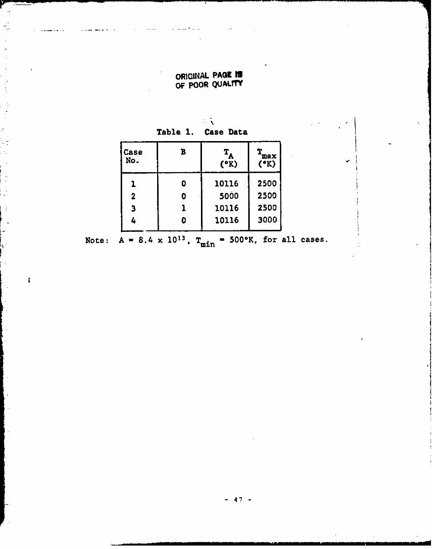
_. ORIGINALPAGEIIIOF POORQuPa.rrY

Table 1. Case Data

case s TA Tmax• No. (°K) (oK)

! 1 0 10116 2500

2 0 5000 250O

_i 3 1 10116 25004 0 10116 3000

I! Note: A - 8 4 x I0_s Tm - 500°K, for all cases.

• ' in

- 47-

:_,,, Jr, i f Ill III ............................................. ii ................................................ --"

- 48 -

i

.. 49

111"-

.able 4 - 2 l%ep qlob:_l i,oael

'_ ORIGINAL P_,GE'g_

_ OF POORQUALrTy

- 50 -

_L

OF POOR Q4JALr_

0.2

0.020.03

0.050.0

0.0 0.02 0.04 0.06 0.08 0.i0

Figure i" Variation of the reaction rate amplificationratio with mean square fluctuation for

rA = 0.2 , rB = 0.2

0.09

0.6 a

L

Zr'

0.4 -

0,2 -

.0 I I| I I I I

0.0 0.02 0.04 0.06 0.08 0.I0

Figure 3: Variation of hhe reaction rate amplificationratio with mean square fluctuations for

-_A=0.4 , rB--'--0.6

::- OF POOR QUALITY

0.2.

0.0,_.. o I i I

0.0 0.02 0.04 0.06 0.08 0.I0

=, - r_ 2

__ _ Figure 4"- Variation of the reaction rate amplification• ratio with mean square fluctuations for

_='o.'l , _=o.?

.. 1.0 _'_-0.5

_"' - 0.1 "

_._.

i e

__.o:

a2.e,?._0] 2' 0 6

_:... gr'

_ _ 04

1¢-

• 0.2

°

0,0 : ' ' ' , -- l_ ..,,_, 0.0 0.2 0.4 0.6 0.8 1.0

Figure 5: Variation of the reaction rate amplification- ratio with mean species concentrations for

=0.01 , =0.01

• _ _ --_ ....._......... _ ........ , ,._._._,_',.

#,

.._ FIG. 7. CO,;_FARISONOF TE[_E._ATUHE-TIM_ PROFILE

i FOR 37(13) AND TEST SYSTEr_S

• l

_w ........ Ti!_' .: ._ v_'_'_-_'-_-_'T"t'_ _ ' ' " -"_ ""_ ........................ r ..... , ...... 7-, _i

!y

...... • : _ • . . { • . _'l . , . . j . 1 . . _,,t .......... , ..... . ..... IL, . .I ............l:!_ .'', i-_-'. _:_t :t-t__ ]1 :: i" i;i.':-i-:'- :.'._! kit-i _li] !rqi i _]iii_ 194i !4j"

,.-_-.- , • -.._ ............................................ L, t .... r ..... _.... _'_...... _ .......-_ ......................... _ ..... ,F ........................i_i:;i _;!t_':L'-.=.=.-:_, _I., .... , .... i .... . ..... ,.._4. .... ,, .......... , ..... , ,..

' ...... -' : _"- .... li'-i-l-lli I ,_ :'-Y¢-' | !IL l!il llll_IIllJl l]"l)i li i_i]l)- ! Ii.... _ : _ 2 '1" _ " s : - ' ; I 'i" -_ I ,l_ .............] J I i ,' '_ _ ' " " : (__,_..,:II m|I ' " ' I "':,*-'_ ri $ i _ .... I , t i i........ ........... .... , .... ,.._.,,.._, ....

:_-'.,_ui _:._-_|-:-'i _.--, .-,=_"--.L'!-'_4 ! ie,.:.i_-]_-_.-l.i_'="E /::%-_-ii ; -i-:-:-l:_....i _ i"-_i"_-_''_ _'_ - " ....... - ...... _ .............. " I 1........... ? .... ? ...... ? ' ' " " "

............... : ::.'!= ::'i "_- -_ .1:F.I'-: :'.':. :-: :--=--t :=:-" : b_:-_i..-.=._- __::L'_" :.:-i : . :.:: : : :.-; =-:= :.,: : t r: _' : : • ' ' : :: : , : :: "_,T+'=_.: .1-,-t .:: : : :.. : .--:- :_$_:-:-r _. -:...r.: -, . .=-', _: _._,'..... : : :..r= , : : ' :_-.-:.: ::'." :_. . , ............... _ _ - ., , , , _ , , ............ , ..... _ . , • _ • . ................... _ ....... .

" "; ...................... "I .... ', ' ' ' ; ..... _"" ' ", " ..... : ................. ; " "'L °'''" ""

.............: _ '."I .' i _ ' ' ' ........... -F-.... i ._.--_- .... ,.... ...":..--.-:-": ;.=':_ =:--=.

" -- ._ m_'_.. .. i.... "'i;_';' ,', : ;...... ,' ":'' :1',, •;..

i I -': ........................• ''IN ® ...... _'-i _:-_' i 'i ::;; L_'T_:_:_;_ ................. I-_-,_ ;- _. I ....._ -+.................................

"" ' : ' , • , .... ] : ..... _ t I i • • • [ " ....... l ; I, .t= i " • : : : - , i :.:---!. : : : , : ; : ,'."l i.:=" _ " _ _" :

" :. :.- : : : : : : 1 : : 1.1 : "I "l '_- .3.._ . : : ; : :'-- "- "..'"-:'; , .._'.= :1.4 ";- .: _---= -I::"" :. -' ..='_.=: "_.'.._': , "-"."_-"-" '................ ,..... =T-_.... _i ........ _ ...... :_-,_-_-.=-_ .........................

• :. :'.t.: :-: : _ ; : :.----' -".+_..$ ::.: _..!_--=:'I-I-_. I -_._. ---.: _ : _ :--'_--_--._-=--='r" i:_-_--=-:'_'---'_---I_._-:-i°. ---_-------'--t:+.l=-="--'4 ". r_-i :-" ..... l.-'.4=.r" -=. -* ;'

•=-.=:-_ ,.- .... : .... .,- "_ :-=,_v_-2z=-.:_=._..-i:._._=.: .... J----.-==-___- .----=_------=..-=-==_.--,---_----.---=..-_--=.._ .......... , ..................... ..T,..._ ...... _............ .'--T... "''_ ............ _=.=:....:.."'a..... I .............

• .qi_ ................ _-L.-¢--_'-. , ' , ........ _-----_-, m..,-.._. _ ........... +............................... _ .............. _ _-' _'I:::I_="-" ' "_ .............. 2";_'_ ......... "_ ....... _ "-"--"_- ..........

-. _ :=--2-:.i;.!-.---__ -: :=:. =.¢-=-:._'.=.=_ ===• : : •"-: _:= " :-: :-_-,-'=7-1=-_'- .i .

-_ ! " ! "'_ " -4.:-__ -I-_4+4I" - - ...... _._. _._ :== :-; _ _'-"=-=" _;.-"m=: -: .... " ..... ----_--.-"_', ..i_i_i I .i__: ...... ___u__.;G,....... "'" .-- -_--._-_------- , . r---_ _ __

' ' -_-4.,_-_ ....... --------4- ...... ,----_ ._0 • .-- ....... --_ --,-- -o** ...... ----.--.... :.... - ...... ,, ....m_" ___-4-_--- +4.,_-,-----_--_---_---,_ ..... .-.---_-_- ..... - ..... .......-- " :; ;" L£-_--__L'W__T_[ _-;_---_= ...... _' =;--P-- ......4+-' "---_-'-_-9 ' .... - _----- '----F ------

• _.i_ : ' •, : : ,,= • _ _ : _-" ; •i

: t-_l ." : : :. r : -'='-: , :.=_.--;r- -'.=-'.'_,_m_.-__'--='a;--t-_'.:.',-=:=-:-=- :__. = I-._=.. :.==_._ "i :. ;:,..-_---.|'-_ ............. 4 .... .--=-_=

: _,,! :'--::i-_::_-_-T:::L=.---..--t=----i%_::-_¢-_._--==-==.== :--=_=_&£-_- "':'i-_ _=__ := -"- =--._-=-_--=--_-_=:=.• • . ; ....... , ................ .._. ;_-_ _ . =---. - _ .- _-._ ....... _.I _ -, .... -- ......... - .......... -_::-

.'-"f-"P-' --'t" . _ . . I., • ; "-.__-t. ' J "_ _ ' ; * ; - • ; ..... _ ....... J ..... .11.- " _.-L- _-. I _ _ _--Ir-_1- . : : .................... | .. : :- ,=..= .:,_-=-:.-=. -_ _ :. _w _-:.--: :. _: : ; ..._ =_---==.--.---:z.-,---:-,-=-_ .=__ .-.-=:.,=_z.=-z,..t ,-__ :t...__• -.)_ _- t ....... _.,-_ i._.,..... , .... _-'-........ t-..,..., ...... ,, ...... f .... ,-,--, .... _--,--,•-: _:-t, .-: : ] t - __-_ :-_ _ . _._'_-_-: ! _ , I ,-. -.":... ::-_._ _-.-_ _: .- _-_-- _ _ _= .-'-_=-._-_=L[.-__._.___=_=__ t-=-=.--:=

_=.-:.-.

ii """• - . J .... L_-_ ............................... _......... _ _ .......... _ ...........

• -,...-- ........ I ...... "T""" _--"_-- -'_ '_ ....... I _"'+- ...... r-...--..... _--_.,'-'-'--'- ......... _ ..... "'-"-'_.*-.... _ .............. -,---6 ..... ;----_-4 . -- _- ; ..... -; .... _ _ ------_-------_- ..... F-_--T -_--_-- _ _ -, --_- ..... _ .................. : ...... t • .. _ . _ . _ i ....

.................. ; _- _-- , ;-: ..... !-----4-------- .-_.+-,-L+-_-,-+-'_.,-_. _ ...... -_-- ....... .__._2..-_ r_- + ........ .-_--,_-_+-tm--i- '+ ..... i.... -t'_"_---'_.'-'_'i _ , I .; ; t- _ _= '_°-',T--'i--t,'--'_"

i i I I lira i i_l i m m , _._1 . I I L ' I .-. Im._ll o l L . . 1 .... .__-_ , _ __._ 1 _ .4 ....--._._.._ .r _--._t_" J :' - " ! " "_') i ; "_,,_, _ .7 ;_ -"_-=_._ ! _ i_.J} -_ _ _"_t ."_-._---.:.=..,,_._..,.....-:_-=--." ._.-a_-_-r-'=-------._i=T._--_=.L'_,;.J_--._--._--- " _...-_,,a._

i._ Li i __ _ _ .,._ _'b_ _ - _if'_ "!-._ i-I _' _ : ._I _ _.=. __---_.,-._i=-:--_=.:w_"_--_=-_--_-_- :_ i i.'=.-=.-.=_-:--_-----_I -: ; _........ .. .1"3.......... I/_ .......... t-- Tt=_. .... _ _==t=_ _==-=___J....,, , ..... ----"

..... I J i - - ;_ _ -j

l. _ ,_ =IF.r-=-__-2_-_--!=+_.-_r=_ _==!=I_..... : . I ., _, -- _=__=_ -='-.-._± , = _ -:. : =_ _ =,_ , _.----_-_ .._ _--_-_+-._-'--:-+-_.--_--'_ _---4-,H- -_-_; " .r-_-_--_.... _.. _-_ - :.=- .,-..w...w._:-W ..:_.-.m-1-,_'_-''_t--

--_ ---t -_--_ '_-_ I_4H.-__ 6 ,'--1"i-- .... : : :

ORf(_NAL P_(._EI$....

°-

...... .... _..... OF POOR QU/_ft_f

c L

: t_,-i i L I _ _ ,| . q

[-- ..... I!_) ............................................................ = .........

!

i . ' In

.......................................................................

_ :7 _., __

......... .............................................

t ._ .

_: ' _ 0 ,=.i.,,

: _ :c" J,.

'J.,

: /:-_ /_/.a m£ BLo_/OO T ................ / 2.:"- K,

.... _a_l['lA_.PA_._1_ ............................

!. _FF'OO_QU,_.nV .... F" I o'_:. ¢=/.o

1

- 12 "" _L . __ _............. , ......... _ _"_ <" I_ I e" ..._

u

, k._ ,

_-r'_,_ ' " i--,--_L,.L'd,,._.,Ji.l.1,.',L_. ............ --_-_-; .... _.._...._,..._._, ...................... --_"'/._I|ii,__L_ I ......... FIr" i :i :1 i" :q']_" _",'._;_,,_, ........ - "'- " ,,

....... {I '; mill Ir--:: " " `+-