This article was downloaded by: [New York University]On: 11 October 2014, At: 07:24Publisher: RoutledgeInforma Ltd Registered in England and Wales Registered Number: 1072954 Registered office: MortimerHouse, 37-41 Mortimer Street, London W1T 3JH, UK

Applied EconomicsPublication details, including instructions for authors and subscription information:http://www.tandfonline.com/loi/raec20

Efficiency measurement in rotating panel dataAlmas HeshmatiPublished online: 04 Oct 2010.

To cite this article: Almas Heshmati (1998) Efficiency measurement in rotating panel data, Applied Economics, 30:7,919-930, DOI: 10.1080/000368498325354

To link to this article: http://dx.doi.org/10.1080/000368498325354

PLEASE SCROLL DOWN FOR ARTICLE

Taylor & Francis makes every effort to ensure the accuracy of all the information (the “Content”)contained in the publications on our platform. However, Taylor & Francis, our agents, and our licensorsmake no representations or warranties whatsoever as to the accuracy, completeness, or suitability for anypurpose of the Content. Any opinions and views expressed in this publication are the opinions and viewsof the authors, and are not the views of or endorsed by Taylor & Francis. The accuracy of the Contentshould not be relied upon and should be independently verified with primary sources of information.Taylor and Francis shall not be liable for any losses, actions, claims, proceedings, demands, costs,expenses, damages, and other liabilities whatsoever or howsoever caused arising directly or indirectly inconnection with, in relation to or arising out of the use of the Content.

This article may be used for research, teaching, and private study purposes. Any substantial or systematicreproduction, redistribution, reselling, loan, sub-licensing, systematic supply, or distribution in anyform to anyone is expressly forbidden. Terms & Conditions of access and use can be found at http://www.tandfonline.com/page/terms-and-conditions

1 Unbalanced panel data not based on rotating sampling design are discussed in Baltagi (1985) and Wansbeek and Kapteyn (1989).

Applied Economics, 1998, 30, 919 ± 930

E� ciency measurement in rotating paneldata

ALMAS HESHMATI

Department of Economic Statistics, Stockholm School of Economics, Box 6501, S-11383,Stockholm , Sweden

Rotating panel data are used with estimation of stochastic production frontier. Themodel can be viewed as a generalization of the regular production function estimationthat accommodates technical ine� ciency as well as ® rm heterogeneity. In particular,while estimating technical e� ciency for each ® rm over time we control for ® rm-speci® c e� ects and separate them from technical ine� ciency. Estimation of the modelis considered in two steps. In the ® rst step we estimate parameters of the underlyingproduction function using generalized least squares method which are then used in theestimation of technical e� ciency in the second step. As an empirical application weused rotating data on 1425 Swedish dairy farms observed during 1976 ± 1988. Themean technical e� ciency of these farms is found to be 94.5% and 16% of the farms arefully e� cient. Evidence of technical regress about 1% per annum is observed during1976 to 1984.

I . INTRODUCTION

There has been a growing trend, in recent years, to use panel(longitudinal) data in applied econometric work. Apart fromhaving a large number of data points and more e� cientparameter estimates, availability of panel data has the ad-vantage of separating individual- and time-speci ® c e� ectsfrom the combined e� ect which is both individual- andtime-speci ® c (see Hsiao, 1986 and Baltagi and Raj, 1992 forsurveys of panel data models).1

Most of the panel data models are based on the assump-tion that each cross-sectional unit is observed for the sametime periods. However, in the context of sampling surveydata from population of ® rms (farms) or households ± theassumption of observing each of them exactly over the sametime length in unrealistic. An alternative to this is to usea rotating’ sample scheme. In a rotating sample schemesome individuals selected in the previous year are droppedfrom the sample and some new individuals from the popula-tion are added to the sample.

Rotation of a sample may be deliberately pursued by thedata collecting agency because the agency can neither force

nor persuade a randomly selected individual to report morethan once or twice (depending on how time consuming thereporting is). That is the main motivation for rotatingsample is to reduce the degree of non-response which isa major problem in collecting data for a standard panel. Onthe contrary, the rotation principle improves the quality ofdata collected by maintaining the representativeness prop-erty of the selected sample especially when the structure ofthe population changes over time.

Rotating panel data might have a number of limitations.First, the cost of few repeated observations might in eachpoint of time equal the cost of a ® rst observation. Second,the data management and computation of large and un-balanced data sets are complex compared to a purecross-section, time-series or balanced data. Third, the lengthof time observed is long enough to control for ® rm e� ects orto identify additional parameters. Fourth, a short length oftime is not desirable considering consistency of some para-meter estimates. Fifth, errors-in-variabl e models might notbe estimable without external instruments. Finally, omittedvariable bias might not be reduced as it can be in the case inlong panels.

0003 ± 6846 Ó 1998 Routledge 919

Dow

nloa

ded

by [

New

Yor

k U

nive

rsity

] at

07:

24 1

1 O

ctob

er 2

014

2 This special case will be similar to the studies by Biorn (1981), Biorn and Jansen (1982, 1983) in the context of consumer demand inNorwegian households.

Econometric estimation using rotating panel data is con-sidered by Biorn (1981), Biorn and Jansen (1982, 1983) tostudy consumer demand in Norwegian households, byNijman et al. (1991) who consider determination of therelative e� ciency of rotating designs in analysis-of-variancemodels and the optimal choice of rotation period usingmonthly expenditures on food and clothing in 1985 in TheNetherlands, and by Heshmati (1994a) to estimate produc-tion functions for crop producers in Swedish agriculture byincorporating the issues of selectivity bias and heteroscedas-ticity in the error component speci® cation.

The purpose of this study is twofold. First, we develop aneconometric model to estimate a stochastic productionfrontier using rotating panel data. The model can be viewedas a generalization of the regular production function es-timation that accommodates technical ine� ciency as well as® rm heterogeneity. Estimation of the regular productionfunction model becomes a special case of the model we usein this study.2 In particular, while estimating technical e� -ciency for each observation we control for ® rm-speci® ce� ects. Consequently, the estimates of technical e� ciencyare not confounded with ® rm-speci® c e� ects. Second, as anempirical application we examine technical e� ciency of1425 Swedish dairy farms observed during 1976 ± 1988. Wecompare productive performances of these farms acrossdi� erent regions, sizes and over time.

Estimation of the model is considered in two steps. In the® rst step we estimate parameters of the underlying produc-tion function which are then used in the estimation oftechnical e� ciency in the second step. A generalized least-squares (GLS) method is developed to estimate parametersof the production frontier which is represented by a translogfunction. The GLS estimators are consistent. The estimatesof technical e� ciency are conditional on the GLS estimatesobtained in the ® rst step. These e� ciency measures are both® rm- and time-speci® c.

One special characteristic of the Swedish agriculture isthat this sector is heavily regulated with extensive govern-ment intervention in both input and output markets. Thegovernment support programmes and price protection incombination with import restrictions have a� ected alloca-tion of inputs and outputs. Ongoing changes in importrestrictions and the price policy will create new conditionswith decreasing prices leading to deterioration of farm pro-® tability and bankruptcy of ine� cient farms. Informationon the current productive performance of the farms is there-fore useful in order to be able to foresee the consequences ofthese changes. The estimated e� ciency of farms can play animportant role in this context.

The paper is organized as follows. The rotating samplingdesign is described in Section II. This is followed by the

statistical model in Section III. Estimation issues are con-sidered in Section IV. Section V contains discussion of thedata and empiricial results are reported in Section VI. The® nal section contains conclusions of the paper.

II . THE ROTATING SAMPLING DESIGN

The structure of the sample and selection of individuals ina rotating sampling design are as follows: Let all individualsin the population be numbered consecutively. The sample inperiod 1 consists of N1 individuals. In period 2, a fraction,me1 (0 < me1 < N1 ) of the sample in period 1 are replacedby mi2 new individuals from the population. In period 3another fraction of the sample in the period 2, me2

(0 < me2 < N2 ) individuals are replaced by mi3 new indi-viduals and so on. Thus the sample size in period t isNt = (Nt ± 1 - met ± 1 + mit). The procedure of droppingmet ± 1 individuals selected in period t - 1 and replacingthem by mit individuals from the population in period t iscalled rotating sampling. In this framework total number ofobservations and individuals observed are + t= 1 Nt andN1 + + t= 2 mit , respectively.

Such a sampling design with (0< {mit , met}< Nt) resultsin variations in two dimensions. The main variation isalong the cross sectional (individual) dimension due tovariation in annual sample (Nt) from one year toanother which is equal to the di� erence between the rotatingsubsample included, mit, and the subsample excluded,met ± 1 . The other type of variation is along time dimensiondue to variations in the number and the successive timeperiods in which di� erent units are observed. The ® rst typeof variation occurs because the planned and recordedsample sizes do not coincide and di� er from one year toanother. The second type of variation occurs because someunits do not enter in the initial planned period, while someothers are dropped out after being observed for a fewperiods resulting in inequality in time series lengths fordi� erent individuals. The fraction with which the samplesrotate (e.g. 25% per annum) is another source causingvariation along the time dimension in the beginning and atthe end periods.

The sampling design outlined above generates severalspecial cases of interest. The ® rst case is completely overlap-ping (mit = met = 0) sample where the same units are ob-served in all the successive time periods. This model ismostly discussed in the usual panel data literature. Thesecond case corresponds to situations with partly overlap-ping (0 < {mit, met}< Nt) samples. The third case depictsthe incomplete non-overlapping (mit = met = Nt) samples.The units are observed only once and the whole sample is

920 A. HeshmatiD

ownl

oade

d by

[N

ew Y

ork

Uni

vers

ity]

at 0

7:24

11

Oct

ober

201

4

replaced after one period. The rotating sample consi-dered in this study is of the second type where the annualsample, rotation subsample and number of time periodsobserved are variable. We observe variations along bothtime and cross sectional dimensions. The exit and entrytimes for a certain unit are allowed to vary. Inclusion ofnew farms in the sample are randomly chosen. When con-sidering exclusive of farms from the sample, one part of thesample rotates non-randomly according to the rotationscheme while another part rotates randomly because ofnon-response.

II I . THE MODEL

Let the production process of the Swedish dairy farms becharacterized by

Yit = f (Zit, u ) exp (e it) (1)

where Y it is the output of the ith dairy farm observedin period t, f ( .) is the production technology, Z is a vec-tor of K inputs and u a vector of parameters to beestimated. i indexes farm (1, 2, ¼ , F) and t time period(t = 1, 2, ¼ , T i). It is to be noted that t varies with i becausedi� erent farms are observed for di� erent time intervals andlengths. A farm subscript i is not added to t to avoidnotational clutter. e it is the error term which is composed ofthe following three components

e it = m i + n it + t it (2)

where m i is the farm-speci® c e� ect, vit is the statistical noiseand t it ( < 0) is technical ine� ciency. The speci® cation of e itin Equation 2 di� ers from some of the previous studies (forexample, Pitt and Lee (1981), Schmidt and Sickles (1984),Kumbhakar (1987), among others) where technical ine� -ciency is assumed to be time-invariant. This time-invariantassumption makes it impossible to separate technical in-e� ciency from farm-speci® c e� ects. Since the farm-speci ® ce� ects are not necessarily ine� cient which is confoundedwith the e� ects that are ® xed over time, it is quite importantto consider a speci® cation of e it that separates technicaline� ciency from farm-speci® c e� ects as postulated in Equa-tion 2. The speci® cation in Equation 2 allows technicaline� ciency to vary over time (see Cornwell et al. (1990),Kumbhakar (1990) and Battese and Coelli (1992) for somespeci® c forms of time dependence). The formulation inEquation 2 reduces to the form used in Kumbhakar andHjalmarsson (1993) for a completely overlapping paneldata. For a survey on the econometric approach to e� -ciency analysis using panel data see Heshmati (1994b,pp. 1 ± 28).

Using a translog form to represent the underlying pro-duction technology, the relationship in Equations 1 and

2 can be written as

ln Y it = a 0 + a 9 lnZi t + 1/2 lnZ 9itB lnZit + m i + n it + t it

= a 0 + lnXi t g + m i + n it + t it (3)

The stochastic production frontier is obtained fromEquation 3 by setting t it = 0. It is to be noted that technicaline� ciency is time-varying and it is separated from farm-speci® c e� ects.

Let qi = (T i - ti + 1) denotes the number of times the ithfarm is consecutively observed, where ti and T i are the ® rstand the last periods during which farm i is observed. If a unitis observed with interruption then qi = T n, where T n is thenumber of time periods a unit is observed non-consecu-tively. Rewrite Equation 3 in vector form as

Y i = õ a 0 + Xi g + v i + t i (4)

where Y i is a q 3 1 vector, õ is a qi 3 1 vector of ones, and Xiis a qi 3 K* matrix (K* = K(K + 3)/2, K is the number ofinputs) of regressors composed of lnZit, squares and crossproducts of lnZit. That is Y i = (lnY it, lnY i , t+ 1 , ¼ , lnY iT),v i = (m i + n it + m i + n i , t+ 1 + , ¼ , + m i + n iT)9 , and t i =(t it, t i , t+ 1 , ¼ , t iT)9 .

We make the following distributional assumptions on theerror components.

i) m i is i.i.d. N (0, s 2m ),

ii) n it is i.i.d. N(0, s 2n),

iii) t it is i.i.d. N(0, s 2t) truncated at zero from above, and

iv) m i , n i t and t it are independent among themselves as wellas of the input.

The last three assumptions are standard in the stochasticfrontier literature (see, for example, Aigner et al. (1977))based on cross-section data. We are using them in thecontext of rotating panel data. The ® rst assumption is stan-dard in the regular panel data models where a randome� ects model is formulated.

With the above distributional assumptions, the variance-covariance matrix of v i is

V i = E (v 9i v i) = s 2nIqi + s 2

m Jqi (5)

where Iqi is an identity matrix of order qi 3 qi and Jqi isa qi 3 qi matrix of ones. Thus

V ± 1i = (1/s 2

n) [Iqi - (s 2

m /( s 2n + qi s

2m ))Jqi] (6)

Both V i and V ± 1i are used in estimation which is dis-

cussed in the following section.

IV. ESTIMATION

T he generalized least squares method

In view of the problems associated with the MaximumLikelihood (ML) method, we consider the Generalized

E� ciency measurement in rotating panel data 921D

ownl

oade

d by

[N

ew Y

ork

Uni

vers

ity]

at 0

7:24

11

Oct

ober

201

4

Least Squares (GLS) method which gives consistent para-meter estimates. However, the GLS estimates will be lesse� cient compared to the ML estimates. For GLS we rewritethe model in Equation 4 as

Y i = õ a 0 + Xi g + e i = XN

i d + e i (7)

where the variance-covariance matrix of e i is

V *i = s 2nIqi + s 2

m Jqi + s 2t((p - 2)/p )Iqi (8)

Since the variance-covariance matrix V *i is non-scalar,the Ordinary Least Squares (OLS) estimates will be ine� c-ient (although consistent except for a 0 which is inconsistentbecause E (e i) = 0). A more e� cient method of obtainingconsistent estimates of g is to use the GLS. The GLSestimate of d is

d = GLS = 3 +i = 1

XN9iV * ± 1

i XNi 4

± 1

3 +i = 1

XÄ 9iV * ± 1i Y i4 (9)

where V * ± 1i = (1/a2 ) [Iqi - (s 2

m /(a2 + qi s2m ))Jqi], and a2 =

s 2n + ((p - 2)/p ) s 2

t.

The GLS estimate of d = (a 0 , a j , b j k) is equivalent tothe OLS estimate after some transformations on the Y andX variables, viz., Y *it = (1/a) [Y it - {1 - (a/(a2 + qi s

2m )1 /2 )}Y i]

and X*i t = (1/a) [Xit - {1 - (a/(a2 + qi s2m )1 /2 )}Xi] where

Y i = (1/qi) S i = 1 Y it and Xi = (1/qi) S i = 1Xit for each variable.Then perform OLS on the following equation

Y *it = X*it d + e *it (10)

The new error term e *it will be homoscedastic. SinceE (e *i t ¹ 0), a W 0 will be inconsistent. However, a consistentestimate of a 0 can be obtained by making some adjustments.

To de® ne the data transformations in Equation 10 esti-mates of s 2

m , s 2n

and s 2t

are to be obtained ® rst. Theseparameters can be consistently estimated from the followingmoment equations

i) m2 = Var(e it) = s 2n + s 2

m + ((p - 2)/p ) s 2t

ii) m3 = third moment of e it = - Ï 2/p ((4 - p )/p ) s 3t

iii) mw2 = Var(e it - e Å i) = s 2n + ((p - 2)/p ) s 2

t

where the sample moments are obtained from the OLSresiduals, eit (including the intercept a 0 ) from Equation3 and e Å i is de® ned as e Å i = (1/qi) S t= 1 e it.

Consistent estimates of a 0 are obtained from a à 0 = ek+( Ï 2/p ) s W

t, where ekis the sample mean of eit over the entire

sample.The Methods of Moment (MOM) based on the OLS

residuals is one alternative to the ML method in estimatingthe variance components. In rotating panel data the mainproblem in using ML method is in evaluating the multivari-ate normal cumulative distribution function (cdf) ± the order

of which depend on the number of times a farm is observed.There is no guarantee that estimate of each of the variancecomponents will be non-negative (see Kumbhakar, 1992 fordetails). Our GLS method gives consistent parameter esti-mates, but less e� cient compared to the ML estimates. Thegain in using GLS is that one avoids to impose strongdistributional assumptions on the error components. Koopand Mullahy (1993) ® nd the Corrected OLS approach basedon the MOM principle and GMM reasonable alternativeestimators to the ML. GMM has the advantages of beingeasier than ML and potentially e� cient relative to MOMand also robust relative to ML. The GMM method pro-duces results which are, in general, di� erent from those ofMOM estimates. However, in the present case we are usingmoments estimate in the second stage where there are noregressors. Therefore, the GMM and MOM estimates arenot di� erent.

Estimation of technical ine� ciency

Consider the pdf of t i give e i, i.e.

f ( t i | e i) = f ( t i, e i)/ f (e i)

= [exp{ - 1/2(t i - mt i) 9 V

± 1i (t i - m

t i)}/

(2p )qi/2 | V i |1 /2 F ( - V 1 /2

i mt i)], t i < 0 (11)

which is the pdf of a multivariate normal (with mean mt i, and

variance-convariance matrix V i) truncated at zero fromabove.

One can use the modal value of t i, mt i, as a point estimator

of t i. The modal value is frequently used in applied e� ciencystudies. It can be interpreted as the ML estimator of t iconditional on the parameter estimates associated withe (Jondrow et al., 1982). m

t i can be derived by maximizing thejoint density of t and v with respect to t and v , subject tothe constraint that v - t = e (see Materov, 1981 for details).The expression for m

t i is

mt i = (s 2

t/( s 2

n + s 2t)) [Iqi - (s 2

m /( s 2n + s 2

t

+ qi s2m ))Jqi] e i, if m

t i < 0

= 0 if mt i > 0 (12)

V. THE DATA

Description of the rotating sample

The data used in this study are part of an annual nationalsurvey of the farm economic conditions of agriculture(JEU), carried out by the Statistics Sweden (SCB). Thesurvey is aimed at providing data that serves as a base forthe annual price negotiations between the representatives of

922 A. HeshmatiD

ownl

oade

d by

[N

ew Y

ork

Uni

vers

ity]

at 0

7:24

11

Oct

ober

201

4

the consumers and producers regarding the regulated partof the Swedish agriculture. The annual survey includes some1000 unincorporated small and medium sized family farmsout of a population of 30 000 to 35 000 farms during theperiod 1976 ± 1988. These farms have an arable land of 20 to100 hectares in the plain districts and 20 to 50 hectares inthe forest and northern districts. A strati® ed random sampleof farms was obtained using the Farm Register in agricul-ture and forestry as the sampling frame. The strati ® cation offarms was according to the production area in direct pro-portion to the total number of farms within the area, cattleunits and the area of arable land.

Each chosen farm is planned to participate in the surveyfor four years with a regeneration rate of 25% every year.The main reason for SCB to apply rotating sampling designis to reduce the degree of non-response and the desire tomaintain the property of the representativeness in theselected sample. The annual degree of non-response hasbeen kept unchanged at the low level of 10 ± 12% of thesample. During the period under investigation there havebeen major changes in the property of representativeness ofthe farms due to changes occurred in the structure of pro-duction and population of farms. The area under cultivationand the number of farms has declined by 3.6% and 22.9%,respectively. The distribution of land by size shows that landbelonging to farms with less than 30 hectares has declinedover time whereas land belonging to farms holding morethan 50 hectares has gone up. Somewhat similar pattern isobserved in the distribution of number of farms underdi� erent size groups. The percentage of farms with land lessthan 20 hectares has increased. These changes are mainlycaused by the rapid technological change and regionaldi� erences in productivity and farming conditions. The ideaof rotation has been helpful in capturing changes in thestructure of agriculture by taking them into account in theannual strati® ed sampling plan.

The outcome of the rotating sample for farms produ-cing dairy products is given in Table 1. Each of the annualsample is composed of four parts or subsamples. Forexample, in 1980 the sample contains 79, 62, 98, and 74farms. The ® rst three parts (79, 62, and 98) are thosenot replaced during the transition from 1979 to 1980. Thelast subsample contains 74 newly included farms from thepopulation. At the same time 85 farms are excluded fromthe sample in 1979. The di� erence between the excludedpart (85) and the included part (74) corresponds tothe changes in the rotating sample size between these twoperiods, i.e. 313 ± 324 = - 11. This di� erence includesonly the part of the sample where each farm is observedconsecutively for four years, Nrot. The di� erence in thenon-rotating part, Nnon, is due to those farms which arenot observed consecutively. The proportion of farms notobserved consecutively, Nnon, in the total annual sample,Nt, varies from 11.2 to 22.6% with an average of 18.7per cent.

Description of the variables

The observed farms in our sample do not all produce thesame outputs or use the same inputs. We have classi® ed thedairy farms’ production activities and resources used intoseveral output and input categories common to all dairyfarms under consideration. To identify the dairy farms wede® ne Y M as the total income generated from production ofmilk delivered to dairy processing plants (99%) and solddirectly (1%). If Y M is positive for a farm, it is classi® ed asa dairy farm. Since these farms are involved in some otherproduction activities, we de® ned an aggregate measure ofoutput from the dairy sector of a farm represented by Y D.Y D is total income from production of milk, beef, pork,lamb, wool, poultry and other dairy products. The share ofmilk, Y M, in the farm’s aggregate dairy output Y D, is onaverage 73% (see Table 2). The unit of measurement of Y M

and Y D is the Swedish currency SEK (converted to 1980prices using the producer price index for dairy productswhich are regulated).

In the present study we use fodder, material, land, labour,and capital as inputs in the production of dairy products. Inaddition to these inputs we consider the age of the farmerand time as explanatory variables.

Consumption of feeding stu� s is classi® ed into two maincategories. Concentrate fodder (XC) is the total cost ofpurchased and concentrate fodder produced at the farm,which is measured in 1980 prices using a cost-price index foragricultural requisites. Grass fodder (XG) is the total at thefarm harvest of grass with 16.5% water content in 1000 kg,and is calculated by multiplying the land used in the pro-duction of grass by the annual average harvest for theproduction area in which the farm is located.

The land variable is also classi® ed into two types of land.Farming land (XF) involves arable land and pasture land(XP) includes the area used for pasture, both given inhectares.

The labour variable (XL) is the total cost of family andhired labour in the production of dairy products only.Labour includes all animal husbandary activities such as:feeding, milking, cleaning, management, fencing and otherservices. Labour cost (measured in SEK) is transformed toconstant 1980 prices using a cost price index for labour inagriculture.

The capital variable (XK) is user cost of capital equipmentincluding depreciation, maintenance, insurance and net in-terest rate costs. The user cost of capital covers the capitalequipment of machinery, inventory and building. The rateof depreciation applied to machinery equipment was be-tween 14 and 17%. Di� erent rates was used depending onthe size of the farm and the di� erences in intensity of capitaluse. A rate of 3.7% was used for farm buildings and 11%was used for inventories. XK is transformed to constant 1980prices using a cost price index for capital equipment inagriculture.

E� ciency measurement in rotating panel data 923D

ownl

oade

d by

[N

ew Y

ork

Uni

vers

ity]

at 0

7:24

11

Oct

ober

201

4

Table 1. Rotating dairy farms economics survey data, 1976 ± 1988

Year Rotating subsamples Nrot

1976 109 100 85 ± ± ± ± ± ± ± ± ± ± ± 294 88.8 37 11.2 331 6.81977 109 100 85 79 ± ± ± ± ± ± ± ± ± ± 373 86.7 57 13.3 430 8.81978 ± 100 85 79 62 ± ± ± ± ± ± ± ± ± 326 77.4 95 22.6 421 8.61979 ± ± 89 79 62 98 ± ± ± ± ± ± ± ± 324 78.3 90 21.7 414 8.51980 ± ± ± 79 62 98 74 ± ± ± ± ± ± ± 313 78.8 84 21.2 397 8.11981 ± ± ± ± 62 98 74 82 ± ± ± ± ± ± 316 80.6 76 19.4 392 8.01982 ± ± ± ± ± 98 74 82 94 ± ± ± ± ± 348 81.5 79 18.5 427 8.71983 ± ± ± ± ± ± 74 82 94 74 ± ± ± ± 324 78.5 89 21.5 413 8.41984 ± ± ± ± ± ± ± 82 94 74 55 ± ± ± 305 78.8 82 21.2 387 7.91985 ± ± ± ± ± ± ± ± 94 74 55 49 ± ± 272 77.9 77 22.1 349 7.11986 ± ± ± ± ± ± ± ± ± 74 55 49 113 ± 290 80.1 72 19.9 362 7.41987 ± ± ± ± ± ± ± ± ± ± 55 49 113 57 273 86.1 31 13.9 317 6.51988 ± ± ± ± ± ± ± ± ± ± ± 49 113 57 219 87.6 31 12.4 250 5.1

Nqi 218 300 340 316 248 392 296 328 376 296 220 196 339 114 3977 81.3 913 18.7 4890 100ti 1976 1976 1976 1977 1978 1979 1980 1981 1982 1983 1984 1985 1986 1987T i 1977 1978 1979 1980 1981 1982 1983 1984 1985 1986 1987 1988 1988 1988qi 2 3 4 4 4 4 4 4 4 4 4 4 3 2

Nqi Sum of the subsamples with rotation according to the sampling plan.Nrot Annual part of the sample with rotation according to the sampling plan.Nnon Annual part of the sample not rotating according to the sampling plan.Nt Annual total sample size, Nt = (Nrot + Nnon).ti First time observed.T i Last time observed.qi No of times farm i is observed, qi = (T i - ti + 1).

Dow

nloa

ded

by [

New

Yor

k U

nive

rsity

] at

07:

24 1

1 O

ctob

er 2

014

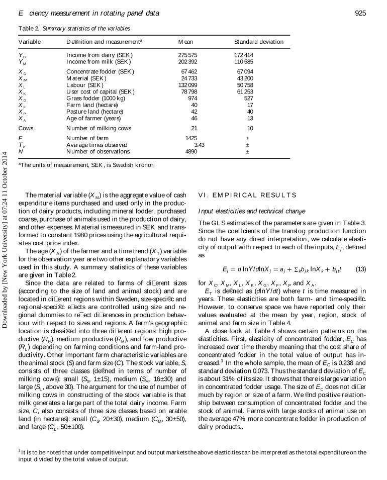
Table 2. Summary statistics of the variables

Variable De® nition and measurementa Mean Standard deviation

Y D Income from dairy (SEK) 275 575 172 414Y M Income from milk (SEK) 202 392 110 585

XC Concentrate fodder (SEK) 67 462 67 094XM Material (SEK) 24 733 43 200XL Labour (SEK) 132 099 50 758XK User cost of capital (SEK) 78 798 61 253XG Grass fodder (1000 kg) 974 527XF Farm land (hectare) 40 17XP Pasture land (hectare) 42 40XA Age of farmer (years) 46 13

Cows Number of milking cows 21 10

F Number of farm 1425 ±T n Average times observed 3.43 ±N Number of observations 4890 ±

aThe units of measurement, SEK, is Swedish kronor.

3 It is to be noted that under competitive input and output markets the above elasticities can be interpreted as the total expenditure on theinput divided by the total value of output.

The material variable (XM) is the aggregate value of cashexpenditure items purchased and used only in the produc-tion of dairy products, including mineral fodder, purchasedcoarse, purchase of animals used in the production of dairy,and other expenses. Material is measured in SEK and trans-formed to constant 1980 prices using the agricultural requi-sites cost price index.

The age (XA) of the farmer and a time trend (XT) variablefor the observation year are two other explanatory variablesused in this study. A summary statistics of these variablesare given in Table 2.

Since the data are related to farms of di� erent sizes(according to the size of land and animal stock) and arelocated in di� erent regions within Sweden, size-speci® c andregional-speci ® c e� ects are controlled using size and re-gional dummies to re¯ ect di� erences in production behav-iour with respect to sizes and regions. A farm’s geographiclocation is classi® ed into three di� erent regions: high pro-ductive (RH), medium productive (RM), and low productive(RL) depending on farming conditions and farm-land pro-ductivity. Other important farm characteristic variables arethe animal stock (S) and farm size (C). The stock variable, S,consists of three classes (de® ned in terms of number ofmilking cows): small (SS, 1 ± 15), medium (SM, 16 ± 30) andlarge (SL, above 30). The argument for the use of number ofmilking cows in constructing of the stock variable is thatmilk generates a large part of the total dairy income. Farmsize, C, also consists of three size classes based on arableland (in hectares): small (CS, 20 ± 30), medium (CM, 30 ± 50),and large (CL, 50 ± 100).

VI . EMPIRICAL RESULTS

Input elasticities and technical change

The GLS estimates of the parameters are given in Table 3.Since the coe� cients of the translog production functiondo not have any direct interpretation, we calculate elasti-city of output with respect to each of the inputs, Ej , de® nedas

Ej = d lnY / d lnXj = a j + S kb j k lnXk + b j tt (13)

for XC, XM, XL, XK, XG, XF, XP and XA .ET is de® ned as ( d lnY / d t) where t is time measured in

years. These elasticities are both farm- and time-speci ® c.However, to conserve space we have reported only theirvalues evaluated at the mean by year, region, stock ofanimal and farm size in Table 4.

A close look at Table 4 shows certain patterns on theelasticities. First, elasticity of concentrated fodder, EC hasincreased over time thereby meaning that the cost share ofconcentrated fodder in the total value of output has in-creased.3 In the whole sample, the mean of EC is 0.238 andstandard deviation 0.073. Thus the standard deviation of EC

is about 31% of its size. It shows that there is large variationin concentrated fodder usage. The size of EC does not di� ermuch by region or size of a farm. We ® nd positive relation-ship between consumption of concentrated fodder and thestock of animal. Farms with large stocks of animal use onthe average 47% more concentrate fodder in production ofdairy products..

E� ciency measurement in rotating panel data 925D

ownl

oade

d by

[N

ew Y

ork

Uni

vers

ity]

at 0

7:24

11

Oct

ober

201

4

Table 3. Generalized least squares parameter estimates

Parameter Estimate Standard error Parameter Estimate Standard error

a b0 0.3453 0.0676 b KK 0.0132 0.0039

a C 0.3199 0.1401 b KG - 0.0123 0.0061a M - 0.1032 0.0919 b KF - 0.0168 0.0132a L 1.0697 0.1556 b KP - 0.0012 0.0022a K 0.3035 0.1208 b KT 0.0040 0.0013a G 0.1376 0.1464 b KA - 0.0021 0.0076a F - 0.2078 0.3741 b GG 0.0035 0.0014a P 0.2165 0.0579 b GF 0.0344 0.0105a T - 0.0962 0.0362 b GP - 0.0044 0.0019a A 0.1247 0.1581 b GT - 0.0028 0.0011b CC 0.0503 0.0030 b GA 0.0037 0.0090b CM - 0.0160 0.0036 b FF - 0.0005 0.0279b CL - 0.0654 0.0109 b FP 0.0091 0.0053b CK - 0.0129 0.0057 b FT - 0.0036 0.0030b CG - 0.0000 0.0060 b FA 0.0070 0.0170b CF - 0.0119 0.0137 b PP 0.0032 0.0015b CP - 0.0022 0.0025 b PT - 0.0001 0.0005b CT 0.0026 0.0012 b PA 0.0026 0.0028b CA - 0.0210 0.0077 b TT 0.0007 0.0002b MM 0.0101 0.0017 b TA - 0.0029 0.0035b ML 0.0121 0.0075 b AA 0.0139 0.0063b MK - 0.0062 0.0039 b RH 0.0395 0.0214b MG 0.0019 0.0039 b RM 0.0173 0.0247b MF - 0.0087 0.0093 b SS - 0.8259 0.0294b MP - 0.0022 0.0016 b SM - 0.3704 0.0237b MT - 0.0015 0.0008b MA 0.0239 0.0057b LL - 0.0079 0.0110b LK - 0.0178 0.0098b LG - 0.0119 0.0106b LF 0.0382 0.0271 s 2

t 0.0114b LP - 0.0146 0.0045 s 2

n 0.0108b LT 0.0054 0.0027 s 2

m 0.0409b LA - 0.0145 0.0140 Observations 4890

bCorrected interceptGlossary of variables:C Concentrated fodderM MaterialL LabourK CapitalG Grass fodderF farm land

P Pasture landT Time trendA Age of farmerRH, RM Regional dummiesSS, SM Size dummies

Unlike the concentrate fodder, the elasticity with respectto grass, EG, has declined over time. Thus there has beena shift in the fodder use from grass to concentrates. The sizeof EG does not di� er much by region or size of animal stock,but it increases with farm size.

Elasticities with respect to both labour, EL, and capital,EK, have increased over time. These increases in the costshares of labour and capital might have happened becauselabour has become relatively more expensive over time andthe production process has become more capital intensive.We ® nd some di� erences in the sizes of EL and EK acrossregions, farm sizes and stock of animals. In particular pro-ductive regions in the south use less labour and capital to

produce the same amount of output. Similar tendencies inthe pattern of EL and EK are observed with respect to farmsize and stock of animal. Large farms with large stock ofanimal are more labour and capital intensive than the smallfarms with small stock of animal.

The elasticity of material, EM, has declined over timewith quite small variations across regions and farm sizes.The variation across stock of animals is somewhat larger.This is because farms with large animal stock apply mech-anized equipment resulting in lower level of material use perherd.

The elasticities of output with respect to farm land, EF,and pasture land EP, have also declined over time. Increased

926 A. HeshmatiD

ownl

oade

d by

[N

ew Y

ork

Uni

vers

ity]

at 0

7:24

11

Oct

ober

201

4

Table 4. Estimates of the marginal output elasticities and technical change (ET) by year, region (R), animal stock (S) and farm size (C)

Year N Concent. Material Labour Capital Grass Land Pasture ET Age

1976 331 0.228 0.059 0.082 0.037 0.052 0.111 0.021 - 0.017 0.1031977 430 0.229 0.059 0.091 0.039 0.051 0.109 0.020 - 0.015 0.1001978 421 0.233 0.058 0.098 0.042 0.049 0.105 0.020 - 0.014 0.0981979 414 0.214 0.061 0.100 0.035 0.045 0.122 0.014 - 0.012 0.0901980 397 0.216 0.060 0.107 0.036 0.042 0.120 0.012 - 0.010 0.0851981 392 0.225 0.056 0.102 0.041 0.039 0.117 0.013 - 0.008 0.0811982 427 0.247 0.042 0.099 0.067 0.033 0.093 0.017 - 0.005 0.0761983 413 0.254 0.040 0.102 0.070 0.032 0.092 0.016 - 0.004 0.0731984 387 0.250 0.038 0.108 0.075 0.028 0.089 0.015 - 0.002 0.0681985 349 0.253 0.012 0.134 0.074 0.017 0.090 0.006 0.005 0.0251986 362 0.245 0.037 0.126 0.084 0.021 0.084 0.015 0.001 0.0631987 317 0.251 0.038 0.125 0.086 0.018 0.082 0.014 0.002 0.0631988 250 0.262 0.034 0.128 0.090 0.016 0.077 0.015 0.004 0.058

RHigh 3081 0.241 0.046 0.104 0.057 0.037 0.099 0.015 - 0.006 0.077RMedium 1043 0.235 0.048 0.107 0.059 0.031 0.106 0.016 - 0.007 0.077RLow 766 0.231 0.046 0.118 0.063 0.034 0.099 0.016 - 0.007 0.075SSmall 1516 0.195 0.053 0.150 0.065 0.036 0.102 0.020 - 0.010 0.085SMedium 2603 0.248 0.044 0.098 0.058 0.034 0.100 0.014 - 0.005 0.074SLarge 771 0.288 0.040 0.053 0.045 0.039 0.100 0.099 - 0.003 0.071

CSmall 1719 0.230 0.051 0.119 0.065 0.027 0.098 0.015 - 0.007 0.075CMedium 2123 0.240 0.045 0.106 0.058 0.036 0.101 0.015 - 0.006 0.076CLarge 1048 0.247 0.042 0.089 0.047 0.047 0.104 0.017 - 0.006 0.081

Mean 4890 0.238 0.046 0.106 0.058 0.035 0.100 0.015 - 0.006 0.077Std dev. 0.073 0.023 0.066 0.031 0.019 0.037 0.014 0.008 0.031

yield per hectare of land in the production of fodder andusage of industrial byproducts as concentrated fodder makeland less and less important. The weather conditions inSweden do not allow use of pasture land for long timeperiods. Thus, EP is expected to be small in magnitude. Thedi� erence in the magnitude of EF with respect to regions,size of farms and animal stock are found to be quite small.

The output elasticity with respect to age, EA , can beinterpreted as the responsiveness of output to age of thefarmer. Since age is directly related to experience in farming,one would expect a positive response of experience to out-put. This is what we ® nd in our data. However, the e� ect ofexperience has declined over time as shown by the decreas-ing values of EA over time.

Finally, the elasticity of output with respect to time, ET, canbe interpreted as the rate of exogenous technical progress. We® nd ET to be negative, although quite small, till 1984 therebymeaning that dairy farms experienced technical regress dur-ing the period 1976 ± 1984 (see Kumbhakar and Hjalmarsson,1993 for a similar result). The situation changed after 1984.Technical progress is observed from 1985 ± 1988 at a very lowrate (less than one per cent per annum).

Farm e� ciency

Now we look at the estimates of technical e� ciency. Meansof these e� ciencies across years, region, farm size and size of

animal stock are reported in the last column of Table 5.Looking at these means, it can be seen that there is notmuch variation in technical e� ciency from one year toanother. However, there is variation in the distribution offarms by e� ciency levels over time. We have not founddi� erences or improvements in mean technical e� ciencyover time. The mean level of technical e� ciency for theentire sample is 94.5% with a minimum of 68% and amaximum of 100%. When classi® ed across regions andfarm-size, we ® nd no signi® cant di� erences in technicale� ciency. However, the mean level of technical e� ciency ishigher for the farms with small animal stock. These ® ndingssuggest that small farms run by family labour are moree� cient.

The frequency distributions of technical e� ciency for theentire sample, for each year, region and sizes show that thepercentage of farms operating below 80% level of e� ciencyvary between 0.3 and 1.5%. It can be seen that only 0.7% ofthe farms were operating at below 80% level of e� ciency.The modal value of technical e� ciency for the entire periodis about 94% and 16.4% of the farms were fully (100%)e� cient. The percentage of fully e� cient farms has increasedafter 1984 (when the percentage of fully e� cient farms wasthe smallest). The e� ciency measures are further brokendown into regions, stocks of animal, and farm-size. It can beseen that there is very little di� erences in e� ciency acrossregions when looked at the percentages of fully e� cient

E� ciency measurement in rotating panel data 927D

ownl

oade

d by

[N

ew Y

ork

Uni

vers

ity]

at 0

7:24

11

Oct

ober

201

4

Table 5. Frequency distribution of technical e� ciency (T EFF) by year, region (R), animals stock (S), and farm size (C)

Interval 00.0 ± 80.0 80.1 ± 82.5 82.6 ± 85.0 85.1 ± 87.7 87.6 ± 90.0 90.1 ± 92.5 92.6 ± 95.0 95.1 ± 97.5 97.6

Year n % n % n % n % n % n % n % n %

1976 3 0.9 3 0.9 11 3.3 12 3.6 28 8.5 42 12.7 77 23.3 65 19.6 43 13.0 47 14.2 0.9431977 0 0.9 4 0.9 12 2.8 23 5.4 31 7.2 50 11.6 79 18.4 72 16.7 64 14.9 95 22.1 0.9491978 5 1.2 6 1.4 8 1.9 12 2.8 28 6.6 40 9.5 62 14.7 68 16.2 72 17.1 120 28.5 0.9551979 4 1.0 9 2.2 11 2.7 19 4.6 28 6.8 53 12.8 85 20.5 70 16.9 62 15.0 73 17.6 0.9431980 2 0.5 11 2.8 6 1.5 12 3.0 26 6.6 35 8.8 77 19.4 85 21.4 53 13.6 90 22.7 0.9501981 6 1.5 6 1.5 16 4.1 19 4.9 37 9.4 47 12.0 84 21.4 71 18.1 56 14.3 50 12.8 0.9381982 1 0.2 4 0.9 10 2.3 20 4.7 31 7.3 67 15.7 106 24.8 83 19.4 48 11.2 57 13.6 0.9421983 3 0.7 4 1.0 6 1.5 10 2.4 24 5.8 48 11.6 95 23.0 78 18.9 80 19.4 65 15.7 0.9501984 2 0.5 10 2.6 9 2.3 16 4.1 32 8.3 70 18.1 103 26.6 73 18.9 41 10.6 31 8.0 0.9341985 4 1.1 5 1.4 10 2.9 16 4.6 24 6.9 51 14.6 87 24.9 73 20.9 40 11.5 39 11.2 0.9381986 1 0.3 3 0.8 11 3.0 13 3.6 28 7.7 55 15.2 91 25.1 74 20.4 41 11.3 45 12.4 0.9421987 1 0.3 6 1.9 7 2.2 7 2.2 24 7.6 44 13.9 74 23.3 68 21.5 45 14.2 41 12.9 0.9441988 1 0.4 2 0.8 3 1.2 2 0.8 13 5.2 26 10.4 61 24.4 54 21.6 37 14.8 51 20.4 0.954

RHigh 23 0.7 40 1.3 72 2.3 105 3.4 232 7.5 400 13.0 696 22.6 604 19.6 429 13.9 480 15.6 0.944RMedium 5 0.5 17 1.6 31 3.0 45 4.3 76 7.3 129 12.4 232 22.2 200 19.2 128 12.3 180 17.3 0.944RLow 5 0.7 16 2.1 17 2.2 31 4.1 46 6.0 99 12.9 153 20.0 130 17.0 125 16.3 144 18.8 0.946

SSmall 9 0.6 13 0.9 21 1.4 43 2.8 77 5.1 154 10.2 237 15.6 241 15.9 273 18.0 448 30.0 0.958SMedium 21 0.8 42 1.6 60 2.3 101 3.9 204 7.8 352 13.5 625 24.0 547 21.0 326 12.5 325 12.5 0.941SLarge 3 0.4 18 2.3 39 5.1 37 4.8 73 9.5 122 15.8 219 28.4 146 18.9 83 10.8 31 4.0 0.929

CSmall 15 0.9 30 1.8 37 2.1 64 3.7 113 6.6 216 12.6 356 20.7 306 17.8 263 15.3 319 18.6 0.946CMedium 13 0.6 35 1.6 59 2.8 81 3.8 158 7.4 289 13.6 450 21.2 413 19.4 273 12.9 352 16.6 0.944CLarge 5 0.5 8 0.8 24 2.3 36 3.4 83 7.9 123 11.7 275 26.2 215 20.5 146 13.9 133 12.7 0.944

Sum 33 0.7 73 1.5 120 2.5 181 3.7 354 7.2 628 12.8 1081 22.1 934 19.1 682 13.9 804 16.4 0.945Cumul. 33 0.7 106 7.2 226 4.6 407 8.3 761 15.6 1389 28.4 2470 50.5 3404 69.6 4086 83.6 4890 100.0

Dow

nloa

ded

by [

New

Yor

k U

nive

rsity

] at

07:

24 1

1 O

ctob

er 2

014

farms. However, one can see substantial di� erences (per-centage wise) among fully e� cient farms of di� erent animalstocks (the farms with 31 or more cows (SL) were found to bethe lowest - 4% compared to 29.6% in SM group). Sim-ilarly, the percentage of fully e� cient farms was found to besomewhat smaller for the large-size farms (CL) (12.7%) com-pared to the small-size (CS) farms (18.6%).

VI I . SUM MARY AND CONCLUSIONS

We have developed a model to estimate technical e� ciencyusing rotating panel data. First, we used a stochastic pro-duction frontier model where the underlying technology isrepresented by a translog function. The neo-classical pro-duction model becomes a special case of our model. Second,we develop GLS method to estimate the parameters ofthe model. Third, the frontier model separates technical in-e� ciency from individual-speci ® c e� ects and technicaline� ciency is allowed to vary over time. Finally, the esti-mates of technical ine� ciency are derived conditional onthe estimated parameters of the production function.Measures of technical ine� ciency are both farm- and time-speci® c.

For an empirical application we used microdata onSwedish dairy farms observed during 1976 ± 1988. Followingare some important conclusions derived from the study.First, we ® nd evidence of technical regress (little more than1% per annum) during 1976 ± 1980. This rate of productivityslowdown was reduced to less than 1% during 1981 ± 1984.However, from 1985 ± 1988 the dairy sector experiencedtechnical progress at a very low (less than 1% per annum)rate.

Second, when looked at the marginal elasticity of outputwith respect to di� erent inputs we ® nd a tendency of use ofmore fodder and less grass over time. On the other hand,labour and capital elasticities increased steadily during theobservation period. Elasticities of output with respect tomaterial, farm and pasture land decreased over time.

Finally, we examined technical e� ciency of individualdairy farms over time. The mean level of technical e� ciencyfor the entire period was found to be 94.5% with a minimumof 68%. About 16% of the farms in the sample were foundto be 100% e� cient. Number of such farms has increasedafter 1984.

The results of our study, especially the farm-level e� cien-cy measures, are useful to policy makers in predicting theconsequences of the recent changes (in progress) in agricul-tural policy. If the future agricultural policy is towardsremoval of price support/subsidy and current protectionistpolicy, then this action will result in an unavoidable struc-tural change. The estimates of farm-level e� ciency willidentify least e� cient farms, their sizes, lines of produc-tion, location, etc., which are subject to bankruptcy orliquidation.

ACKNOWLEDGEMENTS

Financial support from SJRF, HSFR and CEFOS andhelpful comments from Subal C. Klumbhakar and ananonymous referee are acknowledged with gratitude.

REFERENCES

Aigner, D., Lovell, C. A. K. and Schmidt, P. (1977) Formulationand estimation of stochastic frontier production functionmodels, Journal of Econometrics, 6 (1), 21 ± 37.

Baltagi, B. H. (1985) Pooling cross-sections with unequal time-series lengths, Economics L etters, 18 (2), 133 ± 36.

Baltagi, B. H. and Raj, B. (1992) A survey of recent theoreticaldevelopments in the econometrics of panel data, EmpiricalEconomics, 17 (1), 85 ± 109.

Battese, G. E. and Coelli, T. J. (1992) Frontier production func-tions, technical e� ciency and panel data: with application topaddy farmers in India, Journal of Productivity Analysis, 3 (2),153 ± 69.

Biorn, E. (1981) Estimating economic relations from incompletecross-section/time-series data. Journal of Econometrics, 16 (2),221 ± 36.

Biorn, E. and Jansen, E. S. (1982) Econometrics of incompletecross-section/time-series data: Consumer demand in NorwegianHouseholds, 1975 ± 1977, Smafundsokonomiske Studier, Vol-ume 52, Central Bureau of Statistics of Norway.

Biorn, E. and Jansen, E. S. (1983) Individual e� ects in a system ofdemand functions, Scandinavian Journal of Economics, 85 (4),461 ± 83.

Cornwell, C., Schmidt, P. and Sickles, R. C. (1990) Productionfrontier with cross-sectional and time-series variation in e� -ciency levels, Journal of Econometrics, 46, 185 ± 200.

Heshmati, A. (1994a) Estimating random e� ects production func-tion models with selectivity bias: an application to Swedishcrop producers, Agricultural Economics, 11 (2), 171 ± 89.

Heshmati, A. (1994b) Estimating technical e� ciency, productivitygrowth and selectivity bias using rotating panel data: anapplication to Swedish agriculture, PhD Thesis, Departmentof Economics, GoÈ teborg University.

Hsiao, C. (1986) Analysis of panel data, Cambridge UniversityPress, Cambridge, MA.

Jondrow, J., Lovell, C. A. K., Materov, I. S. and Schmidt, P. (1982)On the estimation of technical ine� ciency in the stochasticfrontier production model, Journal of Econometrics, 19 (2/3),233 ± 38.

Koop, R. J. and Mullahy, J. (1993) Least squares estimation ofeconometric frontier models: consistent estimation and infer-ence, Scandinavian Journal of Economics, 95 (1), 125 ± 32.

Kumbhakar, S. C. (1987) The speci® cation of technical and al-locative ine� ciency in stochastic production and pro® t fron-tiers, Journal of Econometrics, 34 (3), 335 ± 48.

Kumbhakar, S. C. (1990) Production frontiers, panel data, andtime-varying technical ine� ciency, Journal of Econometrics,34, 335 ± 48.

Kumbhakar, S. C. (1992) E� ciency estimation using rotating paneldata models. Economics L etters, 38 (2), 169 ± 74.

Kumbhakar, S. C. and Hjalmarsson, L. (1993) Estimation of tech-nical e� ciency and technical progress free from farm-speci® ce� ects: An application to Swedish dairy farms, in T heMeasurement of Productive E� ciency: Techniques and Ap-plications, (eds) H. Fried, C. A. K. Lovell and S. Schmidt,pp. 3 ± 67, Oxford University Press, Oxford.

E� ciency measurement in rotating panel data 929D

ownl

oade

d by

[N

ew Y

ork

Uni

vers

ity]

at 0

7:24

11

Oct

ober

201

4

Materov, I. S. (1981) On full identi® cation of the stochastic produc-tion frontier model, Ekonomika I Matematicheskie Metody,17, 784 ± 88 (in Russian).

Nijman, T., Verbeek, M. and van Soest, A. (1991) The e� ciency ofrotating-panel designs in an analysis-of-variance model. Jour-nal of Econometrics, 49 (3), 373 ± 99.

Pitt, M. M. and Lee, L-F. (1981) The measurement and sources oftechnical ine� ciency in the Indonesian weaving industry,Journal of Development Economics, 9 (1), 43 ± 64.

Schmidt, P. and Sickles, R. C. (1984) Production frontiers andpanel data, Journal of Business & Economic Statistics, 2 (4),367 ± 74.

Wansbeek, T. and Kapteyn, A. (1989) Estimation of the error-components model with incomplete panels, Journal of Econo-metrics, 41 (1), 341 ± 61.

930 A. HeshmatiD

ownl

oade

d by

[N

ew Y

ork

Uni

vers

ity]

at 0

7:24

11

Oct

ober

201

4