Embed Size (px)
Citation preview
EFFICIENCY OPTIMIZATION OF PMSM BASED DRIVE SYSTEM
By
WALEED J. HASSAN
A THESIS
Submitted toMichigan State University
in partial fulfillment of the requirementsfor the degree of
MASTER OF SCIENCE
ELECTRICAL ENGINEERING
2011
ABSTRACT
EFFICIENCY OPTIMIZATION OF PMSM BASED DRIVE SYSTEM
By
WALEED J. HASSAN
The high switching frequency associated with pulse width modulation (PWM) that is com-
monly utilized in controlling the motion of high performance motor drive systems leads to
motor iron losses. In addition to fundamental component, line voltages generated by voltage
source inverters or other types of converters include harmonic components. Minimization of
the harmonic losses leads to higher motor efficiency. Minimization of the harmonic losses
can be accomplished in two stages: first at the design time and the second at the test time.
In the first stage, the motor design can be optimized such that it can work in an efficient
way for a given range of switching frequencies. In the second stage, the operation of the
machine and inverter is optimized such that the total losses of the machine and inverter can
be minimized. By measuring the motor harmonics loss for a given switching frequency, it is
possible to find analytical model that is suitable for estimating the motor harmonics at all
operating points. It is also possible to find the optimum switching frequency, modulation
index, and power factor that minimize the motor-inverter total loss.
Since it is difficult or inaccurate to estimate the harmonic losses of machine through
analytical approach, most researchers resort to finite element analysis (FEA) instead of
analytical solution. The limitation of using finite element software is that it is both time-
consuming and difficult to be implemented in real-time control algorithms. For example, if
it is required to optimize a design that is constructed and analyzed in FEA software, hours
are typically needed to complete such a task.
The proposed work in this thesis is a combination of analytical and numerical meth-
ods that are able to calculate the PMSM harmonic losses at any operating point with less
execution time and adequate accuracy. Moreover, the motor fundamental losses and the
voltage source inverter losses are also modeled such that the inverter-motor efficiency can be
tested for different conditions. Numerical simulation of the field oriented control have been
conducted and results include current, modulation index, power factor, switching frequency
and all the variables in the drive system. Furthermore, Maximum efficiency control strategy
has been chosen such that the drive system can work at the most efficient condition at all
operation points. The proposed work is presented in the context of drive system that is
based permanent magnet synchronous machine (PMSM). However, the proposed method
can be extended to induction motor drive system or any motor use SPWM in controlling the
inverter output voltage.

Copyright byWALEED J. HASSAN2011

I would like to give my deepest appreciation to my parents, who brought me up with their loveand encouraged me to pursue advanced degrees. I would like to give my heartfelt appreciationto my wife, who has accompanied me with her love, unlimited patience, understanding andencouragement. Without her support, I would never be able to accomplish this work.
v

ACKNOWLEDGMENT
First of all, I would like to thank my thesis advisor and mentor Professor Bingsen Wang
for his appreciated effort and support throughout my study in ECE and MSU. Thanks to
him for spending his valuable time in guiding and encouraging me toward my degree. My
thanks extend to my committee members Professor Fang Peng and Professor Joydeep Mitra
for their precious comments and advices. Also, I would like to thank all my friends who
helped me and wished me good luck in my life.
vi
TABLE OF CONTENTS
List of Tables . . . . . . . . . . . . . . . . . . . . . . . . . . . . . . ix
List of Figures . . . . . . . . . . . . . . . . . . . . . . . . . . . . . . x
1 Introduction 1
1.1 Literature Review . . . . . . . . . . . . . . . . . . . . . . . . . . . . . . . . . 11.1.1 Motor Fundamental Losses and Efficiency . . . . . . . . . . . . . . . 21.1.2 Motor harmonic losses . . . . . . . . . . . . . . . . . . . . . . . . . . 2
1.2 Thesis Organization . . . . . . . . . . . . . . . . . . . . . . . . . . . . . . . . 41.3 Summary of Contributions . . . . . . . . . . . . . . . . . . . . . . . . . . . . 5
2 PMSM Harmonics Loss Modeling and Evaluation 6
2.1 Harmonics Iron Losses of Surface Mounted PMSM . . . . . . . . . . . . . . . 72.1.1 Eddy Current Loss . . . . . . . . . . . . . . . . . . . . . . . . . . . . 102.1.2 Hysteresis Loss . . . . . . . . . . . . . . . . . . . . . . . . . . . . . . 11
2.2 SPWM Harmonics Analysis . . . . . . . . . . . . . . . . . . . . . . . . . . . 13
3 Loss Calculation and Analysis of Voltage Source Inverter 16
3.1 Switching Losses of three phase Voltage Source Inverter . . . . . . . . . . . 173.2 Conduction Losses of VSI . . . . . . . . . . . . . . . . . . . . . . . . . . . . 193.3 Total Losses of VSI . . . . . . . . . . . . . . . . . . . . . . . . . . . . . . . . 20
4 PMSM Modeling 22
4.1 Electrical System . . . . . . . . . . . . . . . . . . . . . . . . . . . . . . . . . 244.2 Mechanical System . . . . . . . . . . . . . . . . . . . . . . . . . . . . . . . . 274.3 Transformations . . . . . . . . . . . . . . . . . . . . . . . . . . . . . . . . . . 284.4 PMSM Model . . . . . . . . . . . . . . . . . . . . . . . . . . . . . . . . . . 30
5 Field Orientated Control of PMSM 35
5.1 Introduction . . . . . . . . . . . . . . . . . . . . . . . . . . . . . . . . . . . . 355.2 Field Orientated Control of PMSM . . . . . . . . . . . . . . . . . . . . . . . 36
5.2.1 Space Vector Definition and Projection . . . . . . . . . . . . . . . . . 375.2.1.1 Clarke Transformation . . . . . . . . . . . . . . . . . . . . . 385.2.1.2 Park Transformation . . . . . . . . . . . . . . . . . . . . . . 395.2.1.3 Inverse Park Transformation . . . . . . . . . . . . . . . . . . 39
5.2.2 Overall PMSM Drive System . . . . . . . . . . . . . . . . . . . . . . 415.2.3 Field Orientation Input Parameters . . . . . . . . . . . . . . . . . . . 43
vii
5.3 Sinusoidal Pulse Width Modulation . . . . . . . . . . . . . . . . . . . . . . . 435.3.1 Sinusoidal Pulse Width Modulated Inverter Model . . . . . . . . . . . 445.3.2 Basic Operation of SPWM Inverter . . . . . . . . . . . . . . . . . . . 45
6 Loss Minimization Control Strategy 50
6.1 Modeling Fundamental Losses of PMSM . . . . . . . . . . . . . . . . . . . . 516.2 Condition for Minimized Losses . . . . . . . . . . . . . . . . . . . . . . . . . 53
7 Simulation Results and Discussion 56
7.1 FOC with Loss Minimization Control . . . . . . . . . . . . . . . . . . . . . 577.2 VSI and PMSM Fundamental Losses . . . . . . . . . . . . . . . . . . . . . . 597.3 VSI and PMSM harmonic losses . . . . . . . . . . . . . . . . . . . . . . . . 627.4 Conclusions . . . . . . . . . . . . . . . . . . . . . . . . . . . . . . . . . . . . 677.5 Recommendations for Future work . . . . . . . . . . . . . . . . . . . . . . . 68
Bibliography . . . . . . . . . . . . . . . . . . . . . . . . . . . . . . 70
viii
LIST OF TABLES
3.1 Parameters of the semiconductor devices of the VSI. . . . . . . . . . . . . . . 20
7.1 Machine parameters. . . . . . . . . . . . . . . . . . . . . . . . . . . . . . . . 56
ix
LIST OF FIGURES
2.1 Theoretical harmonic spectra for a three-phase inverter modulated by natu-rally sampled PWM. . . . . . . . . . . . . . . . . . . . . . . . . . . . . . . . 14
3.1 Switching losses of VSI at different load currents. . . . . . . . . . . . . . . . 21
3.2 Conduction losses of VSI at different modulation indices. . . . . . . . . . . . 21
4.1 Dynamic equivalent circuits of PMSM. . . . . . . . . . . . . . . . . . . . . . 23
4.2 Steady state equivalent circuits of PMSM include core loss resistance. . . . . 24
4.3 Dynamic equivalent circuit of PMSM that includes core resistance. . . . . . 25
4.4 Simple schematic model of PMSM. . . . . . . . . . . . . . . . . . . . . . . . 28
4.5 Main SIMULINK window of PMSM model in rotor reference frame. . . . . . 314.6 System 1 in the Main SIMULINK window of PMSM model. . . . . . . . . . 32
4.7 System 2 in the Main SIMULINK window of PMSM model. . . . . . . . . . 32
4.8 System 3 in the Main SIMULINK window of PMSM model. . . . . . . . . . 33
4.9 System 4 in the Main SIMULINK window of PMSM model. . . . . . . . . . 33
4.10 Mechanical system in the Main SIMULINK window of PMSM model. . . . . 34
5.1 Stator current space vector and its components. . . . . . . . . . . . . . . . . 37
5.2 Stator current space vector and its orthogonal components. . . . . . . . . . . 39
5.3 Stator current space vector and its component in the stationary and rotatingreference frames. . . . . . . . . . . . . . . . . . . . . . . . . . . . . . . . . . 40
5.4 Field orientation control diagram. . . . . . . . . . . . . . . . . . . . . . . . . 425.5 Three phase voltage source inverter circuit diagram. . . . . . . . . . . . . . . 47
x
5.6 Voltage waveforms of three-phase voltage source inverter in normalized units. 48
5.7 Three phase voltage source inverter implementation in SIMULINK software. 49
6.1 Steady state equivalent circuits of PMSM include core loss resistance. . . . . 51
6.2 Loss minimization algorithm. . . . . . . . . . . . . . . . . . . . . . . . . . . 54
6.3 Field orientation control diagram incldues loss minimization algorithm. . . . 55
7.1 Dynamic response of phase currents, id and iq of surface mounted PMSM. . 587.2 Torque and speed dynamic response of surface mounted PMSM. . . . . . . . 59
7.3 PMSM efficiency versus speed. . . . . . . . . . . . . . . . . . . . . . . . . . . 607.4 Motor-inverter fundamental losses versus ir∗d at rated speed; (a) PMSM fun-
damental losses; (b) VSI losses; (c) Combined fundamental losses of PMSMand VSI. . . . . . . . . . . . . . . . . . . . . . . . . . . . . . . . . . . . . . 61
7.5 Harmonic losses of PMSM, VSI losses and the combined losses versus switch-ing frequency at rated speed. . . . . . . . . . . . . . . . . . . . . . . . . . . 64
7.6 Total losses of PMSM harmonics loss and VSI losses versus switching fre-quency at different speeds. . . . . . . . . . . . . . . . . . . . . . . . . . . . 65
7.7 PMSM harmonics loss versus modulation index. . . . . . . . . . . . . . . . 66
xi
Chapter 1
Introduction
Loss modeling and control of high performance motor drive system has been one of attractive
research areas since reduced system losses can be translated to lowered energy cost. The
primary objective of this thesis is to calculate the motor inverter loss accurately such that
the motor drive system can operate at maximum efficiency in all operating conditions. A
literature survey has been conducted to include the most up-to-date research results that
are focused on modeling and evaluation of different types of losses of permanent magnet
synchronous machines (PMSMs).
1.1 Literature Review
The state of the art in the following areas is discussed in this section:
• Motor fundamental losses and efficiency
• Motor harmonic losses
1
1.1.1 Motor Fundamental Losses and Efficiency
The efficiency and power density of PMSM have been studied by several researchers [1–
3]. It has been shown that PMSM features significantly higher efficiency than induction
motors when used in adjustable speed drives. Reference [4] provides an analytical method
for estimating the fundamental losses of surface mounted PMSM. Several researchers have
utilized electrical model of PMSM that includes a parallel resistance that accounts for core
losses in high performance applications [5–10]. It can be concluded that both copper and
core losses need to be accounted for in the analysis and control of high performance motor
drives.
1.1.2 Motor harmonic losses
The iron losses of induction motors, permanent-magnet synchronous motors, and switched
reluctance motors have been studied by several researchers [11–17]. Lee and Nam present the
loss distribution of three-phase induction motor fed by a PWM inverter both experimentally
and by use of variable time-step finite element method (FEM) [11]. The results show that
PWM inverters increase the reactive power while decreasing torque. Authors of [12] inves-
tigate experimentally the different losses of three-phase induction machines fed by PWM
inverter. The test results indicate that increasing the converter switching frequency leads to
increased total motor losses, and the loss increase is more pronounced at low speed. Refer-
ence [14] estimates the core loss of flux reversal machines (FRM) under four different modes
PWM using a 2-D time-stepped voltage source FEM. The result of comparing the losses
at the different modes shows that The ON-PWM mode generates higher stator eddy cur-
rent losses. Toda and Ishida investigate the iron losses of a permanent magnet brushless dc
2
motor under different stator core lamination sheets material using FEA and various experi-
ments [15]. Sagarduy et. al. introduce experimental results of iron losses in two non oriented
electrical steels magnetized by using three-phase voltage source inverter carrier based PWM
and three-phase matrix converter space-vector-modulation (SVM) [16]. Their results show
that the eddy current loss in the iron material excited by matrix converter is lower than
that under PWM excitation. In [17] the authors investigate both experimentally and by FE
calculations the iron loss of interior permanent magnet machines driven by PWM inverters.
The investigations show that the carrier of PWM generates the highest iron loss component
under low speed condition.
Experimental inquiry of the iron loss with different PWM parameters is presented in [18–
22]. Authors of [18] study the properties of non-oriented laminations when they are excited by
PWM voltage supply. The results show that the variation of PWM voltage supply parameters
lead to change the properties of laminations. The effect of PWM switching frequency on the
iron loss in soft magnetic material has been investigated in [19]. The experimental results
show that the change in the iron losses is not significant with switching frequency higher
than 4 kHz. Authors of [20] examine the effect of modulation index on the iron losses of
induction motor and wound cores realized with high quality grain oriented magnetic material.
The results show that driving the machine with a variable dc link voltage such that the
modulation index constant and near unity reduces the iron losses. The eddy-current loss
is the dominating loss mechanism according to theoretical research and experiments carried
out in the past [23–26].
The theoretical analysis which study the effect of PWM parameters on the iron losses is
provided in [27]. The authors have found direct analytical expression for a three-phase trans-
3
former and dc motor iron loss with PWM parameters. The symmetrical regular sampling
rule is used to model PWM output voltage and Fourier series expansion has been employed
to extract the harmonics. Also, the authors have assumed that the flux is proportional to
the applied voltage. However, the analytical tool used in [27] cannot be applied in analysis
of sophisticated systems such as three-phase induction motor variable speed drive system or
PMSM variable speed drive system. The inapplicability is due to the following reasons:
• Fourier series provide accurate results only in integer frequency modulating ratios.
• The iron loss caused by carrier waveform fully depends on the phase current and is
controlled by the load, speed, depth of modulation and dc bus voltage. Working on
the voltage instead of current will give inaccurate results.
• It is not enough to calculate the individual effect of each parameter of PWM on the
iron losses. In other words, if it is required to calculate the harmonic losses of variable
speed drive system as a whole under different operating conditions.
1.2 Thesis Organization
Chapter 2 provides analytical model of PMSM harmonic losses based on the armature re-
action field produced by three-phase current of stator winding. Double Fourier series for
naturally sampled sinusoidal PWM (SPWM) has been utilized for evaluation and analysis.
Chapter 3 presents analytical-numerical method of loss calculation for three-phase inverter
controlled by SPWM. Chapter 4 provides complete dynamic model of PMSM that includes
the core loss resistance necessary to calculate the fundamental core loss in steady state. In
Chapter 5, a comprehensive field oriented control model for variable speed drive system is
4
built. The model contains all needed transformation to rotor reference frame and PI con-
troller that are utilized in detailed time-domain simulation. The optimal-efficiency control
strategy is implemented in Chapter 6. The results and conclusion are presented in Chapter
7.
1.3 Summary of Contributions
The main contributions of the thesis work are summarized in the following aspects:
• Modeling the harmonics loss of surface mounted PMSM caused by the non sinusoidal
stator winding currents.
• Calculating the PMSM harmonics loss using double Fourier analysis of SPWM based
on the developed model of the PMSM harmonics loss.
• Modeling the PMSM in dynamic and steady states including the all types of losses
(copper, core, mechanical) and characterizing the efficiency at any operating condition.
• Calculating the losses of the voltage source inverter by analytical model supplied by nu-
merically generated parameters (modulation index, current, displacement angle),such
that the dynamic behaviour of the losses can be tested in all conditions.
• Constructing a complete SIMULINK model that includes what have been mentioned
above in field oriented control system and designing all needed currents and speed
controllers.
• Implementation of the maximum efficiency control strategy, such that the system can
operate under optimal fundamental efficiency at all load, and speed conditions.
5
Chapter 2
PMSM Harmonics Loss Modeling and
Evaluation
The core losses in the machine consist of two components, i.e., hysteresis and eddy current
losses. Both types of core loss are due to time variation of the flux density in the core. The
hysteresis loss is the result of the inherent B−H material characteristics and is proportional
to the product of frequency and flux density with the flux density raised to a power β, which
is generally termed as Steinmetz constant. The value of β ranges from 1.5 to 2.5 and is
dependent on peak operating flux density and material characteristics [28]. In this thesis
work the value of Steinmetz constant is assumed to be 2.
As the flux linkage changes with time, an electromagnetic motive force (EMF) is induced
in core. The induced EMF generates a current in the core depending on the electric con-
ductivity of the core, which will in turn result in losses that are termed the eddy current
losses. The eddy current losses are proportional to the square of the induced EMF and hence
proportional to square of the product of frequency and flux density. The complete expression
6
for core losses in[
Wm−3]
is:
Pcd = Ped + Phd = Ke
∞∑
n=1
(nωr)2B2
p,n +Kh
∞∑
n=1
nωrBβp,n (2.1)
where Ke is the eddy loss proportionality constant that accounts for volume to weight con-
version and all other particular constants are associated with magnetic materials; Kh is the
hysteresis loss density; Bp,n is the peak flux density of the nth-order and fundamental angu-
lar frequency of applied voltage is ωr. In Equation (2.1) when n = 1, the core loss equation
evaluates the losses caused by the fundamental flux density. However, for n = 2 → ∞,
Equation (2.1) evaluates the harmonics loss associated with the harmonic component of the
flux. Evaluation of the fundamental loss of PMSM analytically and in FEA software have
been extensively covered in the literature over the last years. However, the harmonic loss
caused by PWM has not been studied in depth, which is particularly true for induction
and permanent magnet synchronous machines . In the next section an accurate analytical
harmonics loss model based on flux equation by Zhu in 1993 will be introduced [29].
2.1 Harmonics Iron Losses of Surface Mounted PMSM
In this section analytical model for motor harmonic loss is developed based on the work pub-
lished in [29] where the armature reaction field produced by the stator winding is predicted.
The armature reaction field produced by a single-phase stator winding is:
B (α, r, t) = µ◦2W
π
i
δ
∑
v
1
vKsovKdpvFv (r) cos (vα) (2.2)
7
where α = 0 refers to the axis of the phase winding; W is the number of series turns per
phase; and Kdpv = KdvKpv, with Kdv being the winding distribution factor and Kpv being
the pitch factor. Fv (r) is a function dependant on the radius and harmonics order, and
given by:
fv (r) = δv
r
(
r
Rsi
)v 1 +(
Rsir
)2v
1−(
RrRsi
)2v(2.3)
where Rr is rotor radius; δ = g + hm is the effective airgap length with g being the air gap
and hm being radial magnet thickness. When the number of slots per pole per phase is an
integer, the distribution factor Kdv is given by:
Kdv =sin(
q vπQs
)
q sin(
vπQs
) (2.4)
where q is the number of stator slots per pole per phase, and given by:
q =Qs
2Ppm(2.5)
where Qs is the total number of slots; m is the number of phases; and Pp is the number of
pole pairs. The winding pitch factor Kpv is given by:
Kpv = sin(vαy
2
)
(2.6)
8
where αy is the winding pitch. The values of the summation index v is given by:
v = Pp (6c− {±u})
= Pp (6 {0, 1, 2, ..., } − {1, 5, 7, ..., }) + Pp (6 {0,−1,−2, ..., } − {−1,−5,−7, ..., })
u = 1, 5, 7, 11, 13, 17, 19, 23, 25, 29, 35, 37
c = 0± 1± 2± 3, ...
The slot opening factor Ksov is defined as:
Ksov =sin(
vb◦2Rsi
)
v(
b◦2Rsi
) (2.7)
where b◦ is the slot-opening width; Rsi is the stator inner radius. Clearly if the slot-opening
b◦ is very small, i.e., b◦ → 0., then the slot-opening factor approaches unity, i.e, Ksov → 1.
The phase winding currents of PMSM controlled by SPWM contain significant harmonics
and can be expressed by Fourier series as:
ia =∑
n
In sin[
n(
Ppωmt)
+ θn]
(2.8)
ib =∑
n
In sin
[
n
(
Ppωmt− 2π
3
)
+ θn
]
(2.9)
ic =∑
n
In sin
[
n
(
Ppωmt− 4π
3
)
+ θn
]
(2.10)
where θ = Ppωmt, ωm is the rotor mechanical angular frequency in [rad s−1]; and θn is the
harmonic phase angle. Hence the field produced by a three-phase winding can be deduced
9
from (2.2),(2.8),(2,9) and (2,10) as :
B3φ (α, r, t) = Ba (α, r, t) +Bb (α, r, t) +Bc (α, r, t) (2.11)
=
µ◦ 2Wπδ∑
v
1
vKsovKdpvFv (r) ...
{
ia cos (vα) + ib cos(
v(
α− 2π3Pp
))
+ ic cos(
v(
α− 4π3Pp
))}
(2.12)
= {µ◦2W
πδ
∑
n
In∑
v
1
vKsovKdpvFv (r)} sin (nωrt + vα+ θn) (2.13)
where ωr = Ppωm is the electrical rotor angular speed in [rad s−1]; Bp is the maximum
amplitude of armature reaction flux density determined by:
Bp = µ◦2W
πδ
∑
n
In∑
v
1
vKsovKdpvFv (r) (2.14)
2.1.1 Eddy Current Loss
Once the maximum amplitude of the flux density has been defined, which results from the
armature space vector current, the procedure of finding accurate model for core loss is shown
in the following approximate expression.
Ped ∝∑
n
(
nfrBp,n
)2 ∝∑
n
(
nωrBp,n
)2(2.15)
The proportionality expressed in (2.15) represents the first principle in development of the
eddy current loss model, which can be translated to
Ped = Ke
∑
n
(nωr)2B2
p,n (2.16)
10
By plugging equation (2.14) in (2.16) and defining the volume in which the loss are evaluated,
the expression to evaluate eddy core loss as will be reached
(2.17)
Pe = (ρiV )Ped
= (ρiV )Ke
∑
n
(nωr)2B2
p,n
= (ρiV )Ke
∑
n
(nωr)2
(
µ◦2W
πδ
∑
n
In∑
v
1
vKsovKdpvFv (r)
)2
=
(ρiV )Ke
(
µ◦2W
πδ
)2(
∑
v
1
vKsovKdpvFv (r)
)2
∑
n
(nωr)2 I2n
= Kem
∞∑
n=1
(nωr)2 I2n
where ρi is the mass density of the steel core material in [kg m−3]; V is the steel core volume
in [m3]; and their product gives the weight of the core material in [kg]. Kem is defined as:
Kem = (ρiV )Ke
(
µ◦2W
πδ
)2(
∑
v
1
vKsovKdpvFv (r)
)2
(2.18)
2.1.2 Hysteresis Loss
Following the same procedure as the last section, an expression for hysteresis loss can be
reached as presented in equations (2.20) and (2.21):
Phd ∝∑
n
nfrB2p,n ∝
∑
n
nωrB2p,n (2.19)
Phd = Kh
∑
n
nωrB2p,n (2.20)
11
(2.21)
Ph = (ρiV )Phd
= (ρiV )Kh
∑
n
nωrB2p,n
= (ρiV )Kh
∑
n
nωr
(
µ◦2W
πδ
∑
n
In∑
v
1
vKsovKdpvFv (r)
)2
=
(ρiV )Kh
(
µ◦2W
πδ
)2(
∑
v
1
vKsovKdpvFv (r)
)2
∑
n
nωrI2n
= Khm
∞∑
n=1
nωrI2n
The coefficient Khm is defined as:
Khm = (ρiV )Kh
(
µ◦2W
πδ
)2(
∑
v
1
vKsovKdpvFv (r)
)2
(2.22)
The final expression for the core loss in [W] is given by:
(2.23)
Pc = Pe + Ph
= Kem
∞∑
n=1
(nωr)2 I2n +Khm
∞∑
n=1
nωrI2n
Close examination of Kem and Keh shows that they are constant for a given machine design
since they solely depend on the machine dimensions. On the other hand, the core harmonic
loss can be expressed as:
(2.24)
Pc,h = Pe,h + Ph,h
= Kem
∞∑
n=2
(nωr)2 I2n +Khm
∞∑
n=2
nωrI2n
It is clear that the motor harmonics loss can can be fully evaluated if the amplitudes of
current harmonics determined. In the next section the analytical relationship between the
current harmonics sum and the harmonics content of SPWM line voltage will be presented.
12
2.2 SPWM Harmonics Analysis
For three-phase inverter with two-level phase legs, a balanced set of three-phase line-line
output voltages is obtained if the references are displaced by 120◦. Under these conditions,
the line to line voltages are given for naturally sampled PWM by [30]:
vl−l (ω◦,ωc) =
[√3Vdc2 M
]
cos(ω◦t+ π6 ) + ...
[
4Vdcπ
∞∑
m=1
∞∑
n=−∞1mJn
(
mπ2M
)
sin(
[m+ n] π2)
sin(
nπ3
)
]
...
cos(
mωct + n[
ω◦t− π3
]
+ π2
)
(2.25)
Equation (2.25) clearly indicates that the triplen sideband harmonics of the carrier are
cancelled because the term sin(
nπ3
)
will be zero when n = 3, 6, 9, .... Hence the major
significant sideband harmonics that are left will be: fh = fs ± 2f◦, fs ± 4f◦, 2fs ± 5f◦. The
sideband cancellation is not caused by any specific carrier ratio requirement. Therefore,
there is no identifiable benefit with regard to harmonic performance by maintaining an odd
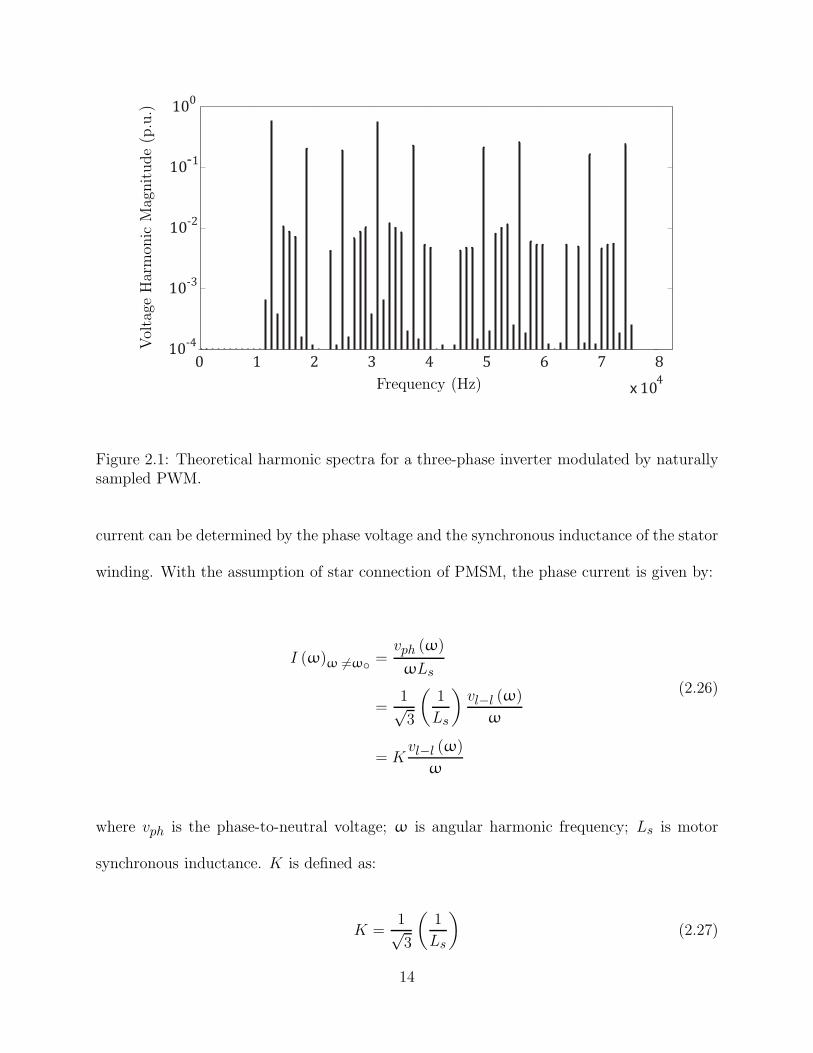
carried/fundamental ratio [30]. Figure 2.1 shows the harmonic components of the line-
line voltage generated by a three-phase inverter switched by double-edge naturally sampled
PWM. The predicted significant sideband harmonics in the first and second carrier group
can be clearly identified. The surface mounted PMSM can be analyzed as a single phase
circuit that consists of series impedance and back emf since the reactances on the d-axis
and the q-axis are identical. At harmonic frequencies 3,6,9 stator resistance and back emf
are neglected so that the motor modeled as synchronous inductance only. The motor phase
13
0 1 2 3 4 5 6 7 8
x 104
10 -4
10 0
10 -3
10 -2
10 -1
Frequency (Hz)
Voltage
Harmon
icMagnitude(p.u.)
Figure 2.1: Theoretical harmonic spectra for a three-phase inverter modulated by naturallysampled PWM.
current can be determined by the phase voltage and the synchronous inductance of the stator
winding. With the assumption of star connection of PMSM, the phase current is given by:
(2.26)
I (ω)ω 6=ω◦ =vph (ω)
ωLs
=1√3
(
1
Ls
)
vl−l (ω)
ω
= Kvl−l (ω)
ω
where vph is the phase-to-neutral voltage; ω is angular harmonic frequency; Ls is motor
synchronous inductance. K is defined as:
K =1√3
(
1
Ls
)
(2.27)
14
Plugging equation (2.25) in equation(2.26) yields:
∣
∣Im,n(ω)∣
∣
ω 6=ω◦ =
∣
∣
∣
∣
∣
K
[
4Vdcπ
∞∑
m=1
∞∑
n=−∞
1
ωm,n
1mJn
(
mπ2M
)
sin(
[m+ n] π2)
sin nπ3
]∣
∣
∣
∣
∣
(2.28)
Alternatively, Equation (2.28) can be expressed as a function of harmonic frequency:
∣
∣Im,n(f)∣
∣
f 6=f◦ =
∣
∣
∣
∣
∣
(
1
2π√3Ls
)
[
4Vdcπ
∞∑
m=1
∞∑
n=−∞
1
fm,n
1mJn
(
mπ2M
)
sin(
[m+ n] π2)
sinnπ3
]∣
∣
∣
∣
∣
(2.29)
Let ωm,n be defined as:
(2.30)ωm,n = 2πfm,n
= 2π (mfsw + nf◦)
where fsw is the inverter switching frequency and f◦ is the motor fundamental frequency.
The motor harmonics loss discussed in the last section is incomplete since the current
harmonics sum was not defined yet. After the current harmonics amplitudes in determined
by (2.28) or (2.29), the motor harmonic core loss is readily determined as the following:
(2.31)
Pc,h = Pe,h + Ph,h
= Kem
∞∑
m=1
∞∑
n=−∞
(
ωm,n
∣
∣Im,n
∣
∣
f 6=f◦
)2+Khm
∞∑
m=1
∞∑
n=−∞ωm,n
(
∣
∣Im,n
∣
∣
f 6=f◦
)2
15
Chapter 3
Loss Calculation and Analysis of
Voltage Source Inverter
The research effort in this thesis is to optimize not only the PMSM efficiency, but also
the drive system as a whole after the estimation of voltage source inverter loss has been
studied. The majority of harmonic losses of the motor, which is caused by PWM carrier
frequency, can be minimized by increasing the inverter switching frequency. Nonetheless,
the inverter switching loss will concurrently increase, as detailed in the subsequent section.
Therefore, for achieving global optimization of the system, one needs to define the value of
the optimal frequency that minimizes the motor harmonic loss and inverter losses together.
The aim of this chapter is to provide analytical model for the calculation of power losses in
IGBT-based voltage source inverter used in PMSM drive system. The inverter parameters
of the semiconductor switches in the inverter have been extracted from the data sheets of
FAIRCHILD, RURG5060 and HTGT30N60A4 modules.
A number of different methods have been proposed to estimate the losses of voltage source
16
inverters. The first is based on the complete numerical simulation of the circuit by specific
simulation programs with integrated or parallel-running losses calculations. The second is
to calculate the electrical behaviour of the circuit based on analytical behaviour model [31].
For accurate estimation of the losses during the transient time and all operating conditions,
a hybrid model has been developed. In this model, the operating conditions that are resulted
from the numerical simulation of the motor drive system are utilized in the analytical model.
The losses in a power-switching device consist of conduction losses, switching losses and
off-state blocking loss. The off-state blocking loss is negligible compared to other two types of
loss, and is given by the product of the blocking voltage and the leakage current. Switching
losses and conduction losses will be analyzed in detail in the following sections.
3.1 Switching Losses of three phase Voltage Source
Inverter
For the subsequent calculations a linear loss model for power semiconductors devices is
assumed. Switching loss energy Es will be linearly scaled as the following:
Es = Esr ·V
Vr· I
Ir(3.1)
where Esr is the rated switching loss energy that is typically given in the device data sheet
for reference commutation voltage Vr and reference current Ir while V and I represent the
actual commutation voltage and current respectively. The rated switching energy can be
defined as the summation of on, off states of each power semiconductor device. For one pair
17
of IGBT and freewheeling diode, Esr is given by
Esr = Eon,I + Eoff,I + Eoff,D (3.2)
where Eon,I and Eoff,I are the turn-on and turn-off energies of the IGBT, respectively;
Eoff,D is the turn-off energy of the power diode due to reverse recovery current. The result
of plugging (3.2) in (3.1) Es is:
Es =(
Eon,I + Eoff,I + Eoff,D
)
· VVr
· I
Ir(3.3)
The power loss Psr is related to the energy loss Esr as by
Esr = Psr · T (3.4)
where T is the switching period. The equation for the switching loss Pls of a VSI with
sinusoidal ac line current and with IGBT switching devices is given by:
Pls =6
π· fs · (Eon,I + Eoff,I + Eoff,D) · Vdc
Vr· ILIr
(3.5)
where fs is the VSI switching frequency; Vdc is the dc link voltage and IL is the peak value
of the ac line current that is assumed sinusoidal.
18
3.2 Conduction Losses of VSI
In contrast to the switching losses, the conduction losses are directly depending on the
modulation function [31]. In [32–35] formulas for reckoning the conduction losses depending
on the modulation function are presented. Reference [36] provides extensive information
on definition of a certain modulation function by the distribution of the duty cycles for
the two different zero vectors. With the knowledge of the relevant modulation function the
conduction losses Plc,I of a single semiconductor IGBT are expressed by equation:
Plc,I =VCE,0
2π·IL∫ π
0sin(ωt)· 1 +M(t)
2·dωt+
rCE,0
2π·I2L∫ π
0sin2(ωt)· 1 +M(t)
2·dωt (3.6)
Likewise the conduction loss that is associated with each diode Plc,D can be written as:
Plc,D =VF,0
2π· IL
∫ π
0sin(ωt) · 1−M(t)
2·dωt+
rF,0
2π· I2L
∫ π
0sin2(ωt) · 1−M(t)
2·dωt (3.7)
The sum of the total conduction losses Plc for all twelve semiconductor devices is determined
by
Plc = 6 ·(
Plc,I + Plc,D)
(3.8)
For the carrier based PWM method equations (3.6) and (3.7) turn into expressions (3.9) and
(3.10) [1].
Plc,I =VCE,0
2π· IL
(
1 +M · π4
· cos (φ))
+rCE,0
2π·(
π
4+M
(
2
3· cos (φ)
))
(3.9)
Plc,D =VF,0
2π· IL
(
1− M · π4
· cos (φ))
+rCE,0
2π·(
π
4−M
(
2
3· cos (φ)
))
(3.10)
19
where M is the modulation index and φ is the displacement angle between the fundamental
of modulation function and the load current. The total inverter losses at different operation
points will be analyzed in the next section.
3.3 Total Losses of VSI
The total losses of the VSI that is realized with practical semiconductor devices have been
evaluated based on he parameters used in the numerical simulation are listed in Table 3.1.
A plot of the switching loss for a range of switching frequencies is shown in Figure 3.1. It is
Table 3.1: Parameters of the semiconductor devices of the VSI.
Power Devices Parameters
IGBTIref (A) 50 Vref (V ) 600Eon,I (mJ) 0.6 Eoff,I (mJ) 0.966VCE,0 (V ) 1.6 rCE,0 (mω) 15
DioderF,0 (mω) 8 VF,0 (V ) 1.6Eoff,D (mJ) 0.7
clear that the switching loss is proportional to switching frequency and maintains constant
for a given load current and switching frequency. With respect to conduction losses, the
loss depends on load displacement angle, modulation index and load current. Figure 3.2
illustrates the variations of the conduction losses with the load displacement angle under
different loading conditions. The plot of conduction loss equation shows that the loss is
maximized when the displacement angle is zero and decreases as the displacement angle
increases or decreases from zero. In field oriented control of variable speed drive system,
for a given speed command the controller will assign voltage proportional to that speed by
means of modulation action. However, increasing the motor speed requires higher line to
line voltage and causes the motor to draw higher current for constant load torque. In other
20
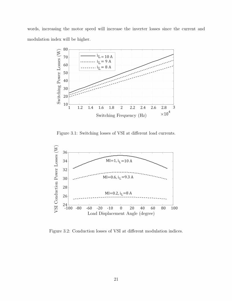
words, increasing the motor speed will increase the inverter losses since the current and
modulation index will be higher.
1 1.2 1.4 1.6 1.8 2 2.2 2.4 2.6 2.8 310
20
30
40
50
60
70
80
iL = 10 AiL = 9 A
iL = 8 A
104
Switching Frequency (Hz) ×
SwitchingPow
erLosses(W
)
Figure 3.1: Switching losses of VSI at different load currents.
-100 -80 -60 -20 -10 0 20 40 60 80 10024
26
28
30
32
34
36
MI=0.2, iL=8 A
MI=0.6, iL=9.3 A
MI=1, iL=10 A
Load Displacement Angle (degree)VSICon
ductionPow
erLosses(W
)
Figure 3.2: Conduction losses of VSI at different modulation indices.
21
Chapter 4
PMSM Modeling
The use of PMSM has rapidly increased in recent years, especially for high performance
applications such as traction, automobiles, robotics and aerospace technology. The PMSM
has a sinusoidal back emf and requires sinusoidal stator currents to produce smooth torque.
The PMSM is very similar to the standard wound rotor synchronous machine except that the
PMSM has no damper windings and its field excitation is provided by permanent magnets
instead of a field winding. Hence the dq-model of the PMSM can be derived from the
well-known model of the synchronous machine with the equations of the damper windings
and field current dynamics removed [37]. The transformation of the synchronous machine
equations from the abc phase variables to the dq variables forces all sinusoidally varying
inductances in the abc frame to become constant in the dq frame.
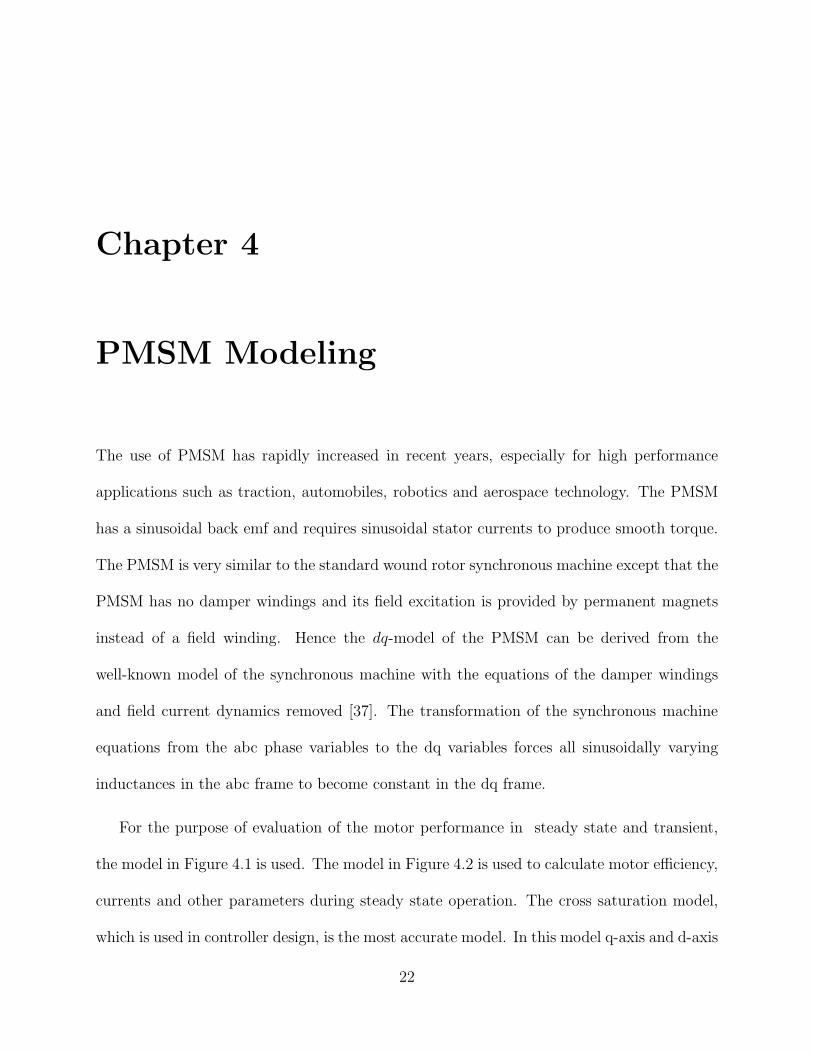
For the purpose of evaluation of the motor performance in steady state and transient,
the model in Figure 4.1 is used. The model in Figure 4.2 is used to calculate motor efficiency,
currents and other parameters during steady state operation. The cross saturation model,
which is used in controller design, is the most accurate model. In this model q-axis and d-axis
22
vrds
vrqs
Rs
Rs
irds
irqs
Ld
Lq
Lqωrioq
Ldωriod
ωrλaf
+
+
+
−
−
−
Figure 4.1: Dynamic equivalent circuits of PMSM.
inductances are functions of id and iq as a result of saturation. A lookup table is typically
needed to store the measured Ld and Lq corresponding to different id and iq combinations.
This model is often used in normalsize size machines in which the iron material more tends
to saturate than big size machines.
To evaluate the motor efficiency as a part of a high performance vector controlled servo
drive numerically in transient, steady state and in all operating points, the selected model is
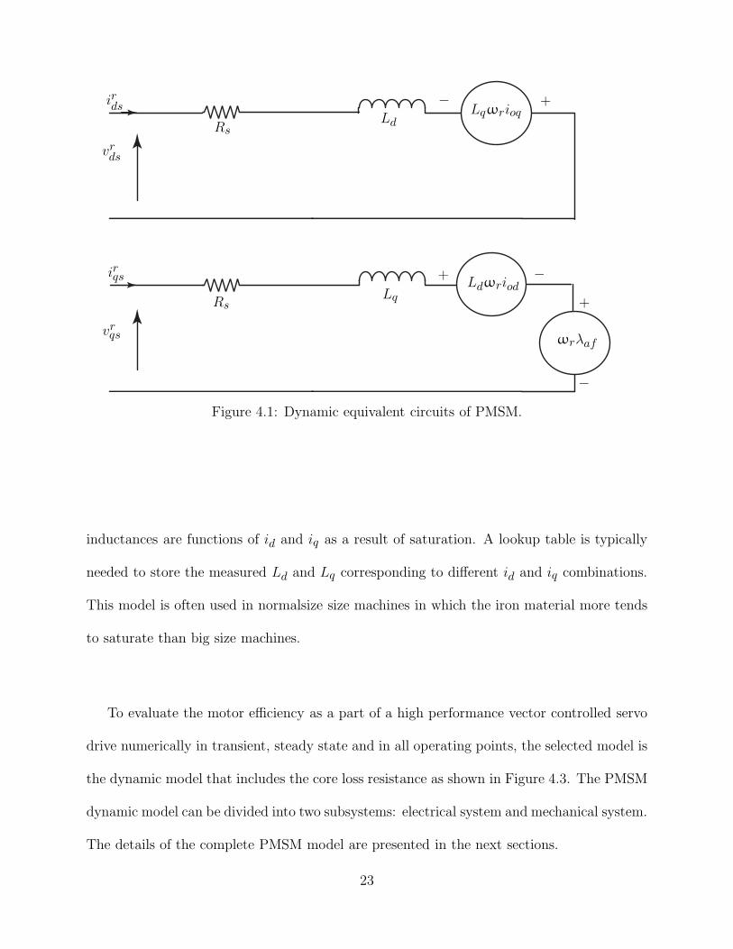
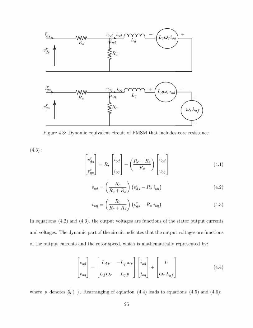
the dynamic model that includes the core loss resistance as shown in Figure 4.3. The PMSM
dynamic model can be divided into two subsystems: electrical system and mechanical system.
The details of the complete PMSM model are presented in the next sections.
23
vrds
vrqs
Rs
Rs
voq
vodirds
irqs
iod
ioq
Rc
Rc
icd
icq
Lqωrioq
Ldωriod
ωrλaf
+
+
+
−
−
−
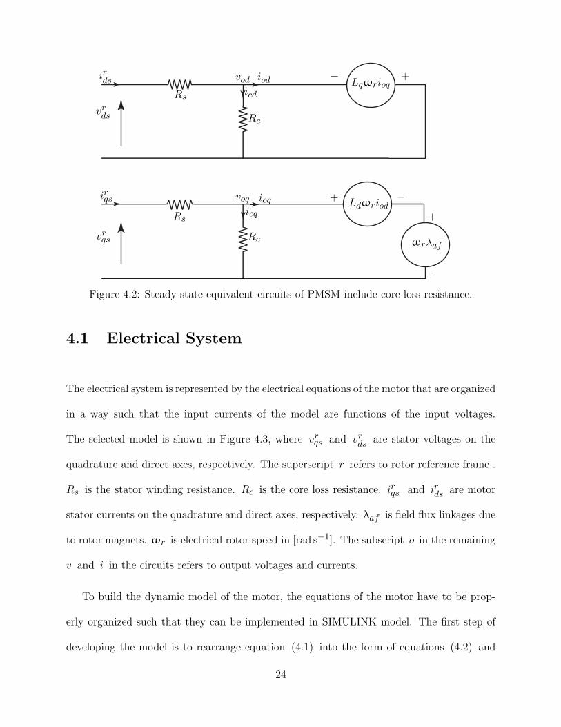
Figure 4.2: Steady state equivalent circuits of PMSM include core loss resistance.
4.1 Electrical System
The electrical system is represented by the electrical equations of the motor that are organized
in a way such that the input currents of the model are functions of the input voltages.
The selected model is shown in Figure 4.3, where vrqs and vrds are stator voltages on the
quadrature and direct axes, respectively. The superscript r refers to rotor reference frame .
Rs is the stator winding resistance. Rc is the core loss resistance. irqs and irds are motor
stator currents on the quadrature and direct axes, respectively. λaf is field flux linkages due
to rotor magnets. ωr is electrical rotor speed in [rad s−1]. The subscript o in the remaining
v and i in the circuits refers to output voltages and currents.
To build the dynamic model of the motor, the equations of the motor have to be prop-
erly organized such that they can be implemented in SIMULINK model. The first step of
developing the model is to rearrange equation (4.1) into the form of equations (4.2) and
24
vrds
vrqs
Rs
Rs
voq
vodirds
irqs
iod
ioq
Rc
Rc
Ld
Lq
icd
icq
Lqωrioq
Ldωriod
ωrλaf
+
+
+
−
−
−
Figure 4.3: Dynamic equivalent circuit of PMSM that includes core resistance.
(4.3) :
vrds
vrqs
= Rs
iod
ioq
+
(
Rc +Rs
Rc
)
vod
voq
(4.1)
vod =
(
Rc
Rc +Rs
)
(
vrds −Rs iod)
(4.2)
voq =
(
Rc
Rc +Rs
)
(
vrqs − Rs ioq)
(4.3)
In equations (4.2) and (4.3), the output voltages are functions of the stator output currents
and voltages. The dynamic part of the circuit indicates that the output voltages are functions
of the output currents and the rotor speed, which is mathematically represented by:
vod
voq
=
Ld p −Lq ωr
Ldωr Lq p
iod
ioq
+
0
ωr λaf
(4.4)
where p denotes ddt ( ) . Rearranging of equation (4.4) leads to equations (4.5) and (4.6):
25
iod =1
Ld
[∫
(
vod + Lq ωr ioq)
dt
]
(4.5)
ioq =1
Lq
[∫
(
voq − Ldωr iod −ωr λaf)
dt
]
(4.6)
It is evident that the output currents are functions of the output voltages, the coupled
output current of the other axis, and rotor speed.
The next step is to calculate the currents of the core loss resistance icd and icq . They
are simply the ratio of output voltage to core loss resistance in each circuit. Since the core
loss resistance is used to calculate the core loss in steady state, the dynamic part of the
output voltage is neglected. In other words, the voltages due to rate of change in Ld and Lq
during the transient are neglected. Equations (4.7) and (4.8) give icd and icq as functions of
the output currents and rotor speed:
icd = −(
Lq
Rc
)
ωr ioq (4.7)
icq =1
Rc
(
λaf + Ld iod)
ωr (4.8)
The last step is to calculate the total rotor currents as:
irds = iod + icd (4.9)
irqs = ioq + icq (4.10)
26
It is worth mentioning that almost all of motor dynamic electrical equations need the motor
electrical speed as an input parameter. The motor electrical speed is proportional to its
mechanical speed that is derived from the mechanical system. The next section details
modeling of the motor speed.
4.2 Mechanical System
The modeling of the motor electrical speed begins at the equation of the electromagnetic
torque generated by the PMSM,
Te =3
2
P
2
[
λaf ioq +(
Ld − Lq
)
iod ioq]
(4.11)
where P is the number of poles. Equation (4.11) generally represents the electromagnetic
torque generated in the two types of PMSM: interior PMSM and surface mounted PMSM.
Surface mounted PMSM can be considered as a special case in which Ld equals Lq. Hence,
the reluctance torque of the electromagnetic torque equals zero.
In order for the motor to operate at a given speed, the electromagnetic torque needs to
overcome all torque components in the opposite direction, which include load torque, friction
torque, and the torque that results from the combined rotor and load moment of inertia.
The torque equation is expressed by:
Te = Jdωm
dt+ Tl +Bωm (4.12)
where J is moment of inertia of the load and machine rotor combined in [kg m2]. ωm is rotor
mechanical speed in [rad s−1]. Tl is load torque in [ N m ]. B is friction coefficient of the
27
load and the machine in [N m rad−1s]. Rearranging of equation (4.12) gives the mechanical
speed:
ωm =1
J
[∫
(Te − Tl − Bωm) dt
]
(4.13)
Finally, the electrical rotor speed is related to mechanical rotor speed by the number of pole
pairs:
ωr =P
2ωm (4.14)
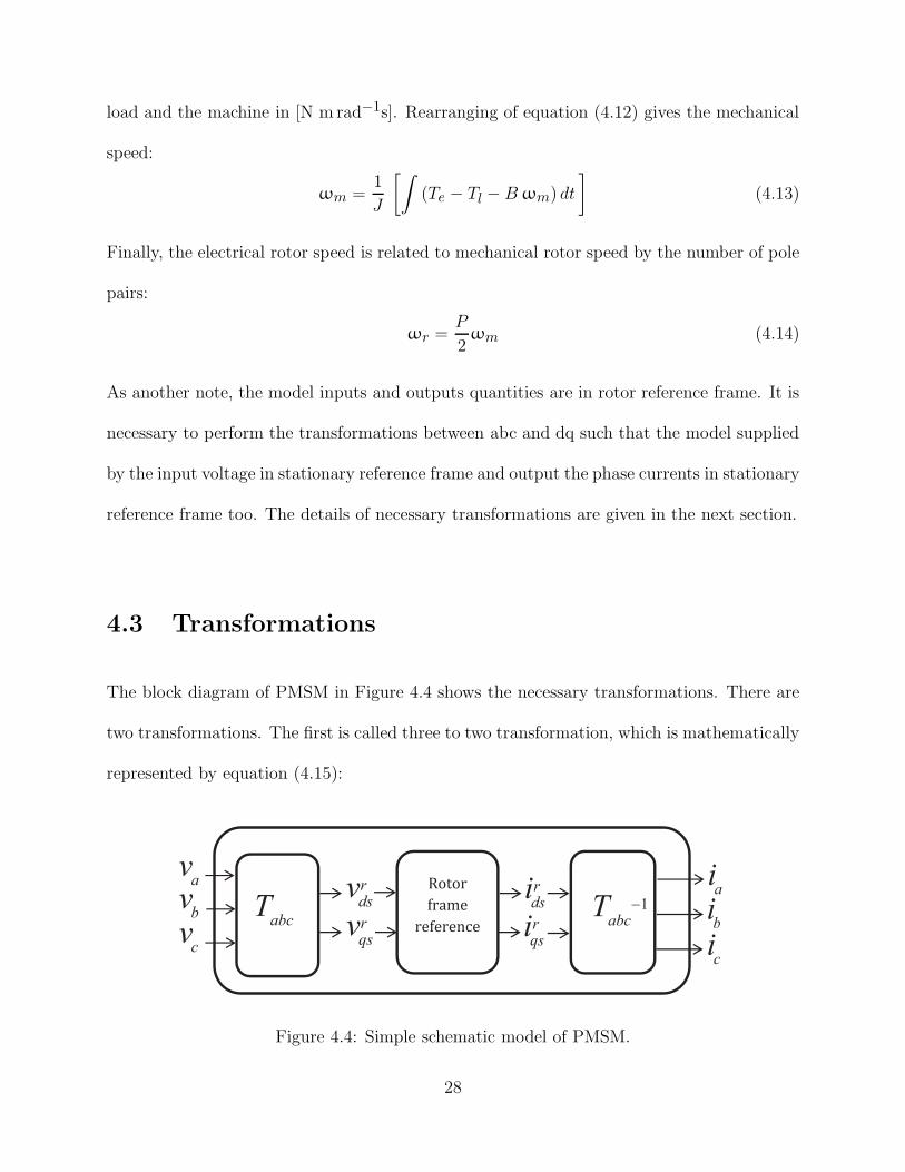
As another note, the model inputs and outputs quantities are in rotor reference frame. It is
necessary to perform the transformations between abc and dq such that the model supplied
by the input voltage in stationary reference frame and output the phase currents in stationary
reference frame too. The details of necessary transformations are given in the next section.
4.3 Transformations
The block diagram of PMSM in Figure 4.4 shows the necessary transformations. There are
two transformations. The first is called three to two transformation, which is mathematically
represented by equation (4.15):
fff
Rotor
frame
reference
rqsv
rdsv
rqsi
rdsia
v
bv
cv
ai
bi
ci
abcT 1
abcT -
Figure 4.4: Simple schematic model of PMSM.
28
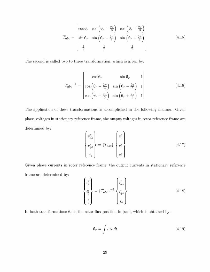
Tabc =
cosθr cos(
θr − 2π3
)
cos(
θr +2π3
)
sin θr sin(
θr − 2π3
)
sin(
θr +2π3
)
12
12
12
(4.15)
The second is called two to three transformation, which is given by:
Tabc−1 =
cosθr sin θr 1
cos(
θr − 2π3
)
sin(
θr − 2π3
)
1
cos(
θr +2π3
)
sin(
θr +2π3
)
1
(4.16)
The application of these transformations is accomplished in the following manner. Given
phase voltages in stationary reference frame, the output voltages in rotor reference frame are
determined by:
vrds
vrqs
v◦
= {Tabc}
vsa
vsb
vsc
(4.17)
Given phase currents in rotor reference frame, the output currents in stationary reference
frame are determined by:
isa
isb
isc
= {Tabc}−1
irds
irqs
i◦
(4.18)
In both transformations θr is the rotor flux position in [rad], which is obtained by:
θr =
∫
ωr dt (4.19)
29
4.4 PMSM Model
The different components of PMSM SIULINK model are described in detail in this section.
This model is part of a complete variable speed motor drive system. The dynamic response
of the model will be introduced after the field oriented control and the maximum efficiency
control strategy are completed in the next chapters.
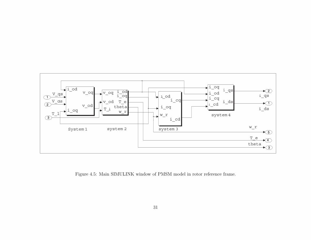
Figure 4.5 shows the main window of PMSM model in rotor frame reference. The model
inputs are vrds, vrqs and the load torque. If the speed and current controllers are designed
accurately, the electromagnetic torque has to be equal the load torque in steady state. The
outputs of the model are speed, torque, position, irds and irqs. The model is organized in four
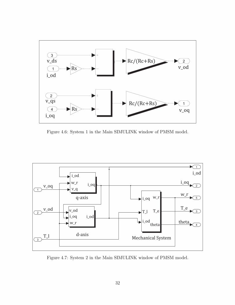
subsystems system 1, system 2, system 3 and system 4. Figure 4.6 illustrates system 1 in
which the equations (4.2) and (4.3) are realized. Equations (4.5), (4.6) and the mechanical
system equations are realized in system 2 as illustrated in Figure 4.7. It is worth mentioning
that the position angle generated by the numerical integration of the mechanical system
serves as input parameter for (4.5) and (4.6). The core loss currents, model input currents
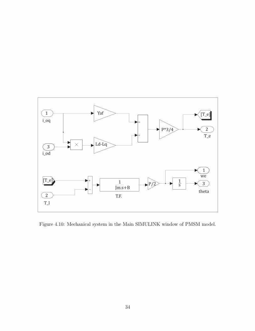
and mechanical system are illustrated in Figures 4.8, 4.9, and 4.10, respectively.
30
1
v_oq
v_od
theta
v_oq
System 1 system 2 system 3
system 4
V_qs
V_ds
T_l
i_od
i_oq
v_od
T_l
i_odi_oq
T_e
w_r
i_od
i_oq
w_r
i_cq
i_cd
i_oq
i_odi_cq
i_cd
i_qs
i_ds
i_qs
i_ds
w_r
T_e
2
3
2
1
5
4
3
theta
Figure 4.5: Main SIMULINK window of PMSM model in rotor reference frame.
31
v_ds
i_od
v_qs
i_oq
Rs
Rs
Rc/(Rc+Rs)
v_oq
v_odRc/(Rc+Rs)
Figure 4.6: System 1 in the Main SIMULINK window of PMSM model.
i_oq
i_od
w_r
T_e
theta
Mechanical System
q-axis
d-axis
v_oq
v_od
T_l
i_oq
i_od
i_oq
T_l
i_od
T_e
w_r
theta
v_od
i_oq
w_r
i_od
w_r
v_q
Figure 4.7: System 2 in the Main SIMULINK window of PMSM model.
32
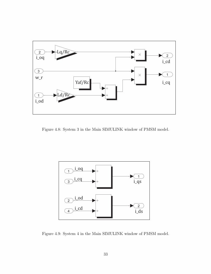
Figure 4.8: System 3 in the Main SIMULINK window of PMSM model.
Figure 4.9: System 4 in the Main SIMULINK window of PMSM model.
33
T.F.
1
Jm.s+B
1s
i_oq
i_od
[T_e]
Yaf
Ld-Lq3
1
2
T_l
P/2
[T_e]
2
T_e
P*3/4
we
theta
1
3
Figure 4.10: Mechanical system in the Main SIMULINK window of PMSM model.
34
Chapter 5
Field Orientated Control of PMSM
5.1 Introduction
Vector control, also known as decoupling or field oriented control, came into the field of ac
drives research in the late 1960s. It was developed prominently in the 1980s to meet the
challenges of oscillating flux and torque responses in inverter fed induction and synchronous
motor drives [28]. Traditionally variable speed electric machines were based on the sepa-
rately excited dc machines. The main reason was due to the high performance dynamic
ability of separately excited dc machines drives that resulted from its ability of independent
control of the flux and torque. The flux is controlled by the field current alone. The field
current is kept constant and hence is the flux. The torque is independently controlled by
the armature current alone. Therefore, this armature current may be treated as the torque-
producing current. In the dc machine, this decoupling is obtained in by orienting the current
in quadrature to the stator flux by use of a mechanic commutator.
In the last three decades, significant advances in the areas of power semiconductor and
35
control technology have led to adjustable speed-drives for ac machines. The mathematical
models for ac machines are inherently more complex than the dc counterparts. More complex
control schemes and more expensive power converters are needed to achieve acceptable speed
and torque control performance. By use of advanced control approaches like field-oriented
control, the dynamic performance at least equivalent to that of a commutator motor can be
achieved. The key to it then lies in finding an equivalent flux-producing current and torque-
producing current in ac machines leading to the control of the flux and torque channels in
them.
To achieve the necessary decoupling, first the machine has to be modeled in space vector
form, where a three-phase machine is transformed into a machine with one winding each on
stator and rotor. The transformed machine resembles an equivalent dc machine. Second, the
ability of the inverter to produce a current vector with controllable magnitude, frequency, and
phase is needed. Both of these features are exploited to make the PMSM drive system a high-
performance drive system with independent control of its mutual flux and electromagnetic
torque [28]. The details are explained in the following sections.
5.2 Field Orientated Control of PMSM
A field-oriented dq control technique is one in which the d- and q-axis components of the
current are controlled independently. Typically one of them is oriented to control the flux
while the other is oriented to control the torque. The next subsections describe in detail the
components that form field oriented controller.
36

5.2.1 Space Vector Definition and Projection
The three-phase voltages, currents and fluxes of ac machines can be analyzed in terms of
complex space vectors [38]. The space vector of the motor input currents in stator reference
frame can be defined as follows. Given the instantaneous currents isa, isb, i
sc, then the complex
stator current vector iss is defined as:
iss = isa + α isb + α2 isc (5.1)
where α = ej 23π. The diagram in Figure 5.1 illustrates the stator current complex space
vector.
iss
αisb
α2isc
isa
Figure 5.1: Stator current space vector and its components.
The depicted space vector current represents three-phase sinusoidal system. It still needs
to be transformed into a rotating coordinate system. This transformation can be accom-
plished in two steps:
• (a, b, c) ⇒ (α, β) Clarke transformation that outputs a two coordinate time variant system.
37
• (α, β) ⇒ (d, q) Park transformation that outputs a two coordinate time invariant system.
The complete description of these transformation will be detailed in the next subsections.
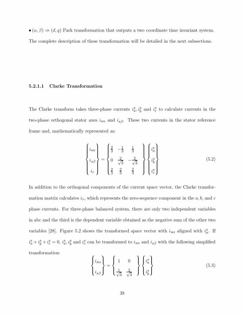
5.2.1.1 Clarke Transformation
The Clarke transform takes three-phase currents isa, isb and isc to calculate currents in the
two-phase orthogonal stator axes isα and isβ . These two currents in the stator reference
frame and, mathematically represented as:
isα
isβ
i◦
=
23 −1
313
0 2√3
− 2√3
23
23
23
isa
isb
isc
(5.2)
In addition to the orthogonal components of the current space vector, the Clarke transfor-
mation matrix calculates i◦, which represents the zero-sequence component in the a, b, and c
phase currents. For three-phase balanced system, there are only two independent variables
in abc and the third is the dependent variable obtained as the negative sum of the other two
variables [28]. Figure 5.2 shows the transformed space vector with isα aligned with isa. If
isa+ isb + isc = 0, isa, isb and isc can be transformed to isα and isβ with the following simplified
transformation:
isα
isβ
=
1 0
1√3
2√3
isa
isb
(5.3)
38
α=a
β
iS
b
c
iSα
iSβ
Figure 5.2: Stator current space vector and its orthogonal components.
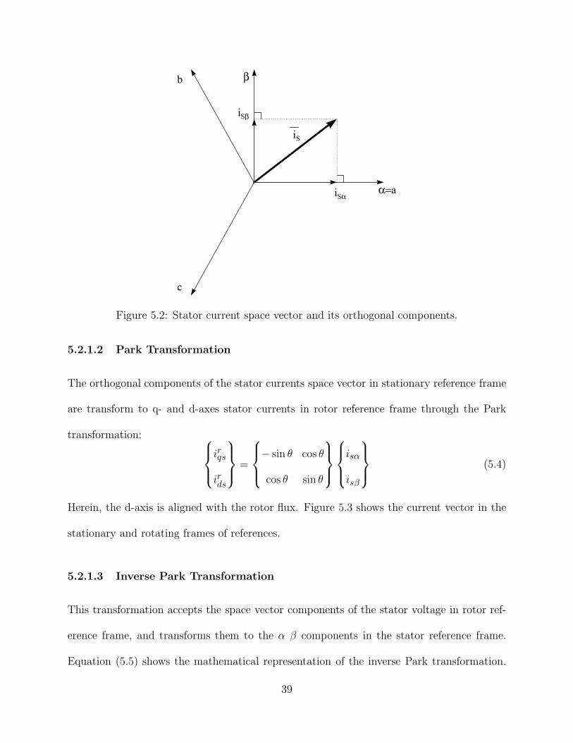
5.2.1.2 Park Transformation
The orthogonal components of the stator currents space vector in stationary reference frame
are transform to q- and d-axes stator currents in rotor reference frame through the Park
transformation:
irqs
irds
=
− sin θ cos θ
cos θ sin θ
isα
isβ
(5.4)
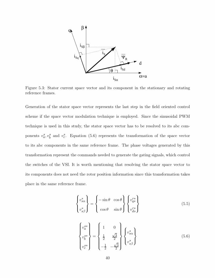
Herein, the d-axis is aligned with the rotor flux. Figure 5.3 shows the current vector in the
stationary and rotating frames of references.
5.2.1.3 Inverse Park Transformation
This transformation accepts the space vector components of the stator voltage in rotor ref-
erence frame, and transforms them to the α β components in the stator reference frame.
Equation (5.5) shows the mathematical representation of the inverse Park transformation.
39
relationship from the two reference frame:
θα=a
β
iS
d
q
iSd
iSq
iSα
iSβ
ΨR
Figure 5.3: Stator current space vector and its component in the stationary and rotatingreference frames.
Generation of the stator space vector represents the last step in the field oriented control
scheme if the space vector modulation technique is employed. Since the sinusoidal PWM
technique is used in this study, the stator space vector has to be resolved to its abc com-
ponents vsa, vsb and vsc . Equation (5.6) represents the transformation of the space vector
to its abc components in the same reference frame. The phase voltages generated by this
transformation represent the commands needed to generate the gating signals, which control
the switches of the VSI. It is worth mentioning that resolving the stator space vector to
its components does not need the rotor position information since this transformation takes
place in the same reference frame.
v∗sα
v∗sβ
=
− sin θ cos θ
cos θ sin θ
vr∗qs
vr∗ds
(5.5)
vs∗a
vs∗b
vs∗c
=
1 0
12
√32
−12 −
√32
v∗sα
v∗sβ
(5.6)
40
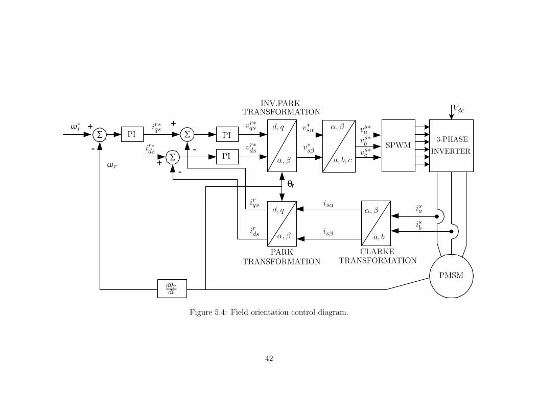
5.2.2 Overall PMSM Drive System
The implementation of the vector-controlled PMSM drive system is described in this section
based on the understanding gained in the previous sections on vector control. The overall
block diagram of the speed-controlled systems is illustrated in Figure 5.4. The first step is to
measure two stator phase currents. These measurements are fed to the Clarke transformation
module. The outputs of this module are isα and isβ . These two components of the space
vector current are the inputs of the Park transformation that gives the current in the d,q
rotating reference frame. The irqs and irds components are compared to the references ir∗ds
(the flux reference) and ir∗qs (the torque reference), respectively. The torque command ir∗qs is
the output of the speed regulator and ir∗ds is the output of the maximum efficiency control
algorithm, which will be further detailed in the next chapter. The outputs of the current
regulators are vr∗qs and vr∗ds , which are applied to the inverse Park transformation. The outputs
of this projection are v∗sα and v∗sβ , which are the components of the stator voltage vector
in the α, β stationary orthogonal reference frame. v∗sα and v∗sβ are also the inputs of the
space vector PWM modulator. However, in SPWM, the outputs of this block are resolved
into components of the voltage space vector, which are subsequently compared with carrier
signals to generate the signals that drive the inverter. It is worth noting that both Park and
inverse Park transformations need the rotor flux position, which means increased complexity
and the cost of ac drive system. The obtaining of the rotor flux position is discussed in the
following subsection.
41
Σ Σ
Σ
- -
-
θr
+ +
+
α, β
α, β
α, β
d, q
d, q
v∗sα
v∗sβ
isα
isβ
vr∗qs
vr∗ds
irqs
irds
dθrdt
PI
PIPI
PARK
TRANSFORMATION
TRANSFORMATIONCLARKE
TRANSFORMATION
ir∗qs
SPWM3-PHASE
INVERTER
INV.PARK
PMSM
isa
isb
Vdc
ω∗r
ωr
a, b
ir∗ds
α, β
a, b, c
vs∗avs∗bvs∗c
Figure 5.4: Field orientation control diagram.
42
5.2.3 Field Orientation Input Parameters
To implement the field oriented controller, two input variables are needed: rotor position and
two of motor stator currents. As described in the last subsections, the transformation from
stator to rotor reference frames and vice versa requires rotor position. The rotor position can
be measured directly by position sensor or by integration of rotor speed since the rotor speed
is equal to the rotor flux speed in PMSM [38]. However, the currents considered as the core
variables of FOC. The currents are measured by current sensor and then sampled by A/D
before received by the controller. In recent years most control algorithms are implemented
in digital signal processor (DSP) because of its ability to generate the triggering signal of the
voltage source inverter at very high switching frequency and its capability of implementation
of even very sophisticated control algorithms.
5.3 Sinusoidal Pulse Width Modulation
In order to investigate the motor harmonics loss caused by static power conversion, the
inverter topology, and control method have to be determined first. Since the power rating
of the PMSM under study is about 3 kW, the three-phase inverter with IGBTs has been
chosen as controlled switches as shown in Figure 5.5. However, there are different control
methods that can be used to control motor speed (by the control of the frequency, amplitude
and phase of motor phase voltages) such as space vector PWM (SVPWM), six-step, and
sinusoidal PWM (SPWM). Despite SVPWM generate less harmonics than SPWM with
higher output fundamental voltage, the spectral analysis of output voltage of SPWM inverter
is a straightforward process by application of double Fourier series expansion. The next
sections highlight the important aspects of controlling the three-phase VSI by SPWM control
43
method.
5.3.1 Sinusoidal Pulse Width Modulated Inverter Model
The VSI consist of three legs connected in parallel, and is supplied with a constant dc voltage
as shown in Figure 5.5. Each leg consists of two IGBT switches connected in series and is
controlled by pluses obtained by the comparison between the reference command and the
triangle carrier waveform. It is important to note that the two IGBTs in the same leg is never
conducting simultaneously since in such shoot-through case high short-circuit current passes
through the leg leads to damage of the inverter module. If ideal transistors in the inverter
module are assumed, then there is no short circuit as long as there is no overlap between the
upper and lower switches. However, practical inverters will need deadtime to avoid shoot-
through since finite time interval is needed for the commutation of these semiconductor
power switches.
The triangle waveform named carrier determines the converter switching frequency. The
frequency of the reference command establishes the desired fundamental frequency of the in-
verter output voltage. The frequency ratio of the carrier waveform to the reference command
is referred to as the frequency modulation ratio. The ratio between the amplitude of the
fundamental component and the amplitude of the carrier signal is called modulation index.
The diodes in the circuit diagram provide paths for currents when a transistor is gated on
but cannot conduct the polarity of the load current [39]. For example, if the load current is
negative when the upper transistor is gated on, the diode in parallel with the upper transis-
tor will conduct until the load current becomes positive at which time the upper transistor
will begin to conduct. The switches of the phase legs are controlled based on the following
44
comparison:
vs∗a ≥ vtr T1 is on
vs∗a < vtr T2 is on
vs∗b ≥ vtr T3 is on
vs∗b < vtr T6 is on
vs∗c ≥ vtr T5 is on
vs∗c < vtr T4 is on
where vs∗a , vs∗b and vs∗c are the reference control commands generated by by control algorithm.
vtr is the triangle waveform. The mathematical derivation of the inverter output phase and
line voltages will be detailed in the next subsection.
5.3.2 Basic Operation of SPWM Inverter
The dc link voltage is assumed constant in the three-phase voltage source inverter shown in
Figure 5.5. The midpoints of the inverter phase-legs are a, b, and c. The inverter output
voltages with respect to negative rail of the dc bus have two output states each:
vag = Vdc for T1 on and T2 off
= 0 for T2 on and T1 off
vbg = Vdc for T3 on and T6 off
= 0 for T6 on and T3 off
vcg = Vdc for T5 on and T4 off
= 0 for T4 on and T5 off
45

They are derived with the assumption that the devices are ideal. The line-to-line voltages
can be derived as:
vab = vag − vbg
vbc = vbg − vcg
vca = vcg − vag
For balanced system in which the sum of currents and voltages equals zero, the phase voltages
can be expressed as the following:
van = 13 (vab − vca)
vbn = 13 (vbc − vab)
vcn = 13 (vca − vbc)
Let the modulation index be defined as:
M =V̂ref
V̂tri(5.7)
If M ≤ 1, the modulation is linear, where the fundamental frequency component in the
output voltage varies linearly with the amplitude modulation index ratio M [40]. From
Figure 5.6, the peak value of the fundamental-frequency component in one of the inverter
legs is:(
V̂ag
)
1= M
Vdc2
(5.8)
46
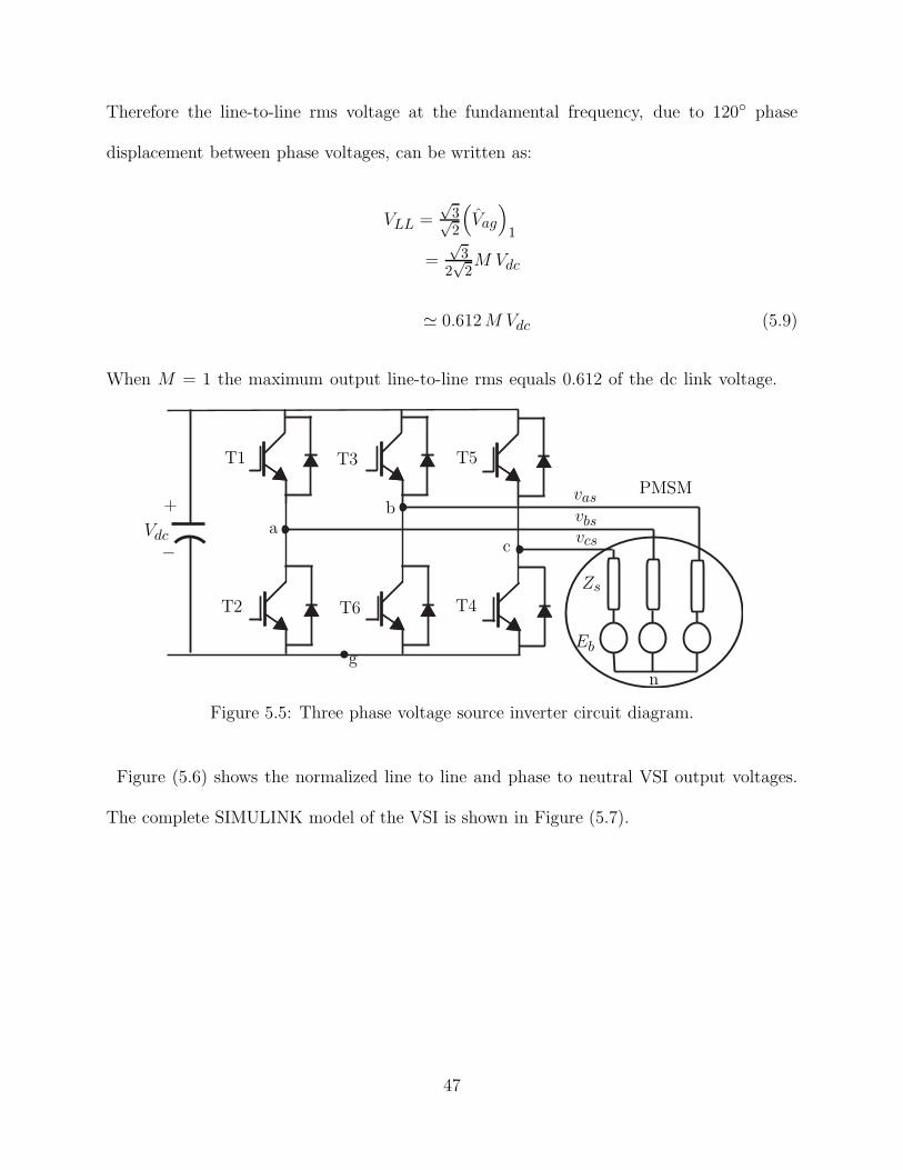
Therefore the line-to-line rms voltage at the fundamental frequency, due to 120◦ phase
displacement between phase voltages, can be written as:
VLL =√3√2
(
V̂ag
)
1
=√3
2√2M Vdc
' 0.612M Vdc (5.9)
When M = 1 the maximum output line-to-line rms equals 0.612 of the dc link voltage.
T1 T3 T5
T2 T4T6
Vdc
vasvbsvcs
Zs
ng
Eb
+
−a
b
c
PMSM
Figure 5.5: Three phase voltage source inverter circuit diagram.
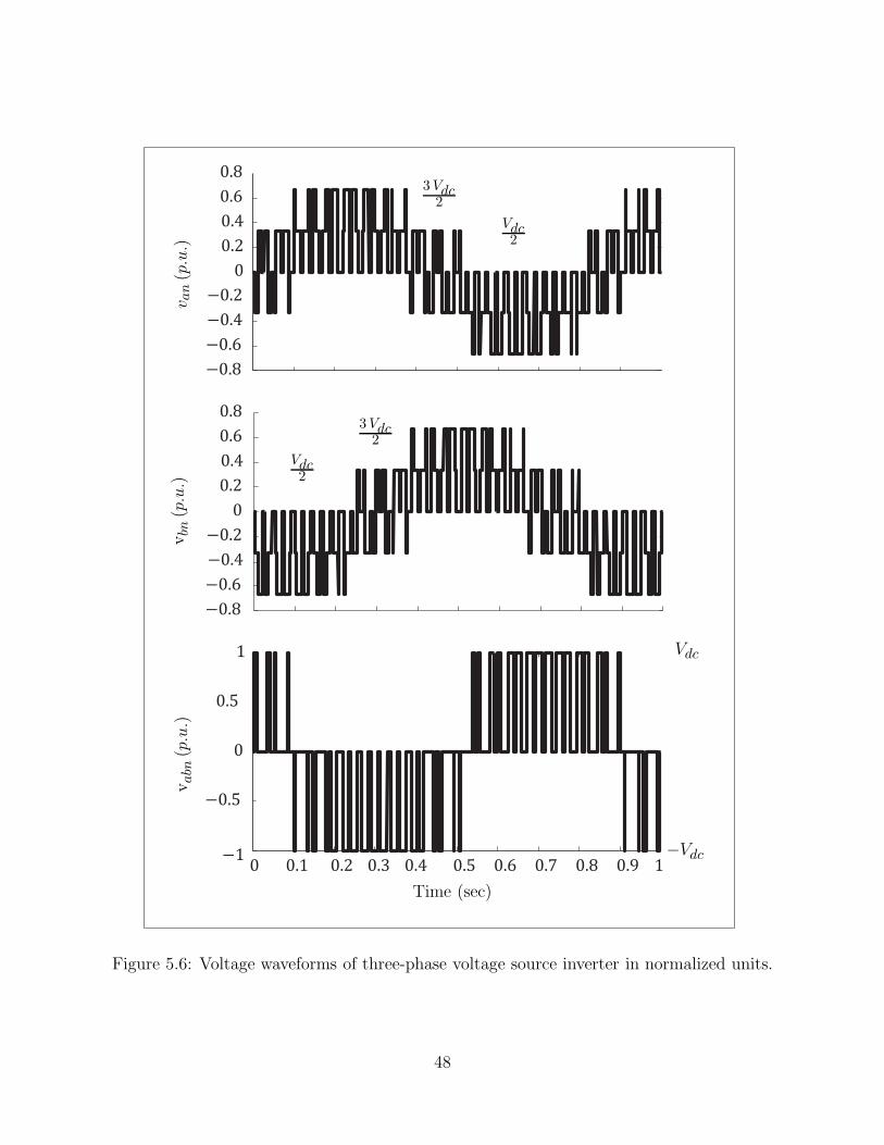
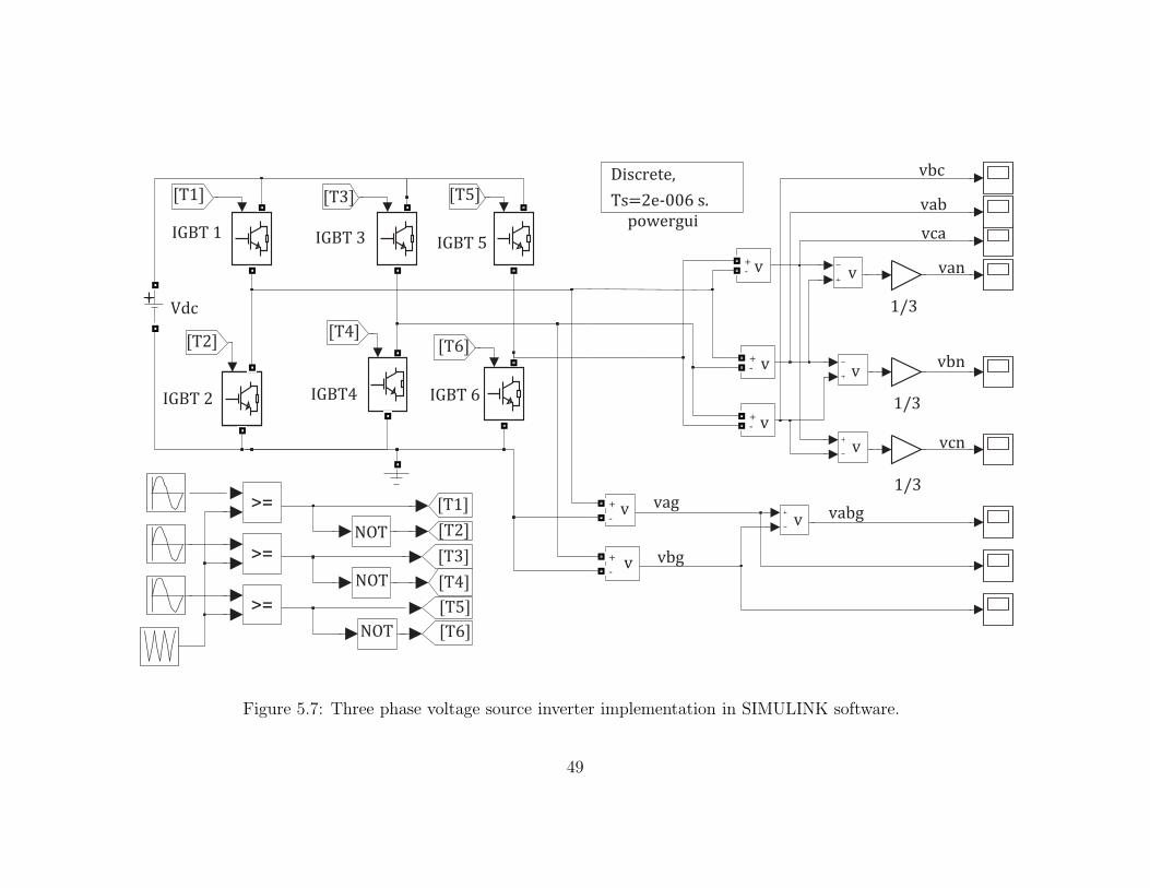
Figure (5.6) shows the normalized line to line and phase to neutral VSI output voltages.
The complete SIMULINK model of the VSI is shown in Figure (5.7).
47
−0.8
−0.6
−0.4
−0.2
0
0.2
0.4
0.6
0.8
−0.8
−0.6
−0.4
−0.2
0
0.2
0.4
0.6
0.8
0 0.1 0.2 0.3 0.4 0.5 0.6 0.7 0.8 0.9 1
0
1
0.5
−1
−0.5
van(p.u.)
vbn
(p.u.)
vabn
(p.u.)
Time (sec)
3Vdc2
3Vdc2
Vdc2
Vdc2
Vdc
−Vdc
Figure 5.6: Voltage waveforms of three-phase voltage source inverter in normalized units.
48
[T2]
[T1] [T3] [T5]
[T4][T6]
[T1]
[T2]
[T3]
[T4]
[T5]
[T6]
NOT
NOT
NOT
Figure 5.7: Three phase voltage source inverter implementation in SIMULINK software.
49
Chapter 6
Loss Minimization Control Strategy
This chapter is focused on the improvement of the efficiency of surface mounted PMSM. The
combined copper losses and iron fundamental losses are minimized through control strategy
developed in [41]. The controllable losses can be minimized by proper choice of the armature
current vector. It is a common practice to set the current id = 0. As a result, the armature
current vector that is in phase with the back EMF is applied. In addition, irreversible
demagnetization of permanent magnets can be avoided [41]. The recent development of the
permanent magnets has brought materials with high coercivity and high residual magnetism.
Therefore, several control methods have been proposed to improve the performance of the
PM motor drives. In such control methods, the d-axis component of armature current is
actively controlled according to the operating speed and load conditions. In the next section,
the basic equations of motor model needed to develop the control algorithm are presented.
50
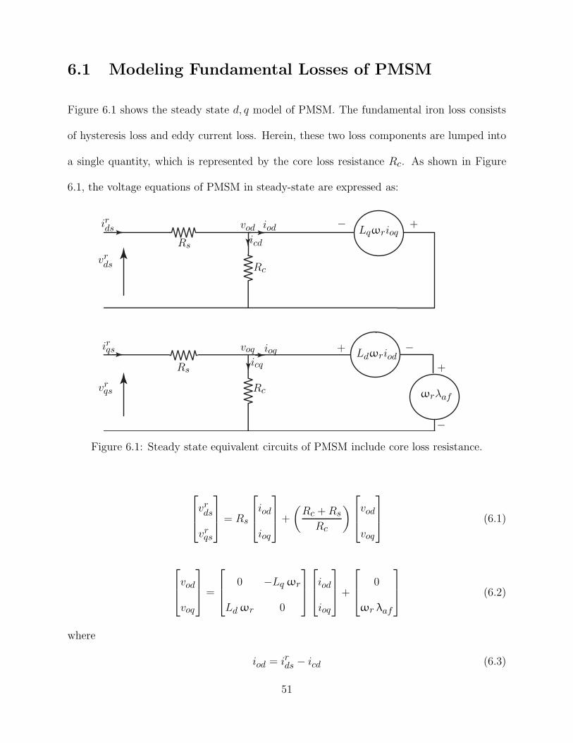
6.1 Modeling Fundamental Losses of PMSM
Figure 6.1 shows the steady state d, q model of PMSM. The fundamental iron loss consists
of hysteresis loss and eddy current loss. Herein, these two loss components are lumped into
a single quantity, which is represented by the core loss resistance Rc. As shown in Figure
6.1, the voltage equations of PMSM in steady-state are expressed as:
vrds
vrqs
Rs
Rs
voq
vodirds
irqs
iod
ioq
Rc
Rc
icd
icq
Lqωrioq
Ldωriod
ωrλaf
+
+
+
−
−
−
Figure 6.1: Steady state equivalent circuits of PMSM include core loss resistance.
vrds
vrqs
= Rs
iod
ioq
+
(
Rc +Rs
Rc
)
vod
voq
(6.1)
vod
voq
=
0 −Lq ωr
Ldωr 0
iod
ioq
+
0
ωr λaf
(6.2)
where
iod = irds − icd (6.3)
51
ioq = irqs − icq (6.4)
icd = −(
Lq
R c
)
ωr ioq (6.5)
icq =1
Rc
(
λaf + Ld iod)
ωr (6.6)
The armature current ia, the terminal voltage va and the torque Te are expressed as:
ia =√
i2d+ i2q (6.7)
va =√
v2d+ v2q
va =
√
(
Rs id −ωr Lq ioq)2
+(
Rs iq +ωr(
λaf + Ld iod))2
(6.8)
Te =3
2
P
2
[
λaf ioq +(
Ld − Lq
)
iod ioq]
(6.9)
The copper loss PCu, the iron loss PFe and the mechanical loss PM , are determined by:
PCu = 32Rs i
2a
= 32Rs
(
i2d + i2q)
=3
2Rs
(
iod −ωrLqioq
Rc
)2
+
(
ioq +ωr
(
λaf + Ldiod)
Rc
)2
(6.10)
PFe =32Rc i
2c
= 32Rc
(
i2cd + i2cq)
=3
2
{
ω2r
(
Lqioq)2
Rc+
ω2r
(
λaf + Ldiod)2
Rc
}
(6.11)
52
PM = Tmωm
= (Bωm)ωm
= Bω2m
= B
(
2
Pωr
)2
(6.12)
The electrical loss PE , the total loss PL, the output power P◦ and the efficiency η are
expressed as:
PE = PCu + PFe (6.13)
PL = PE + PM (6.14)
P◦ = Teωm (6.15)
η =P◦
P◦ + PL× 100 (6.16)
6.2 Condition for Minimized Losses
Substituting (6.10) and (6.11) into (6.13) yields an expression for controllable electrical loss
as a function of ωr, iod and ioq. The variable ioq in these equations can be cancelled by
substituting (6.9) into (6.10) and (6.11). As a result PE can be expressed as a function of
iod, Te and ωr. In the steady state the electrical loss PE is function of iod. Nevertheless,
for surface mounted PMSM Ld = Lq. Hence, simple expression for PE can yield. By
differentiation of PE with respect to iod, the condition for iod that minimizes the controllable
53
losses results as:
∂PE∂iod
= λ3af
(
32P2
)2iod(
RsR2c +ω2
rL2dRs +ω2
rL2dRc
)
+ λ4af
(
32P2
)2Ld(Rs +Rc)ω
2r
∂PE∂iod
= 0
iod = −λaf (Rs +Rc)ω
2rLd
RsR2c +ω2
rL2d(Rs +Rc)
(6.17)
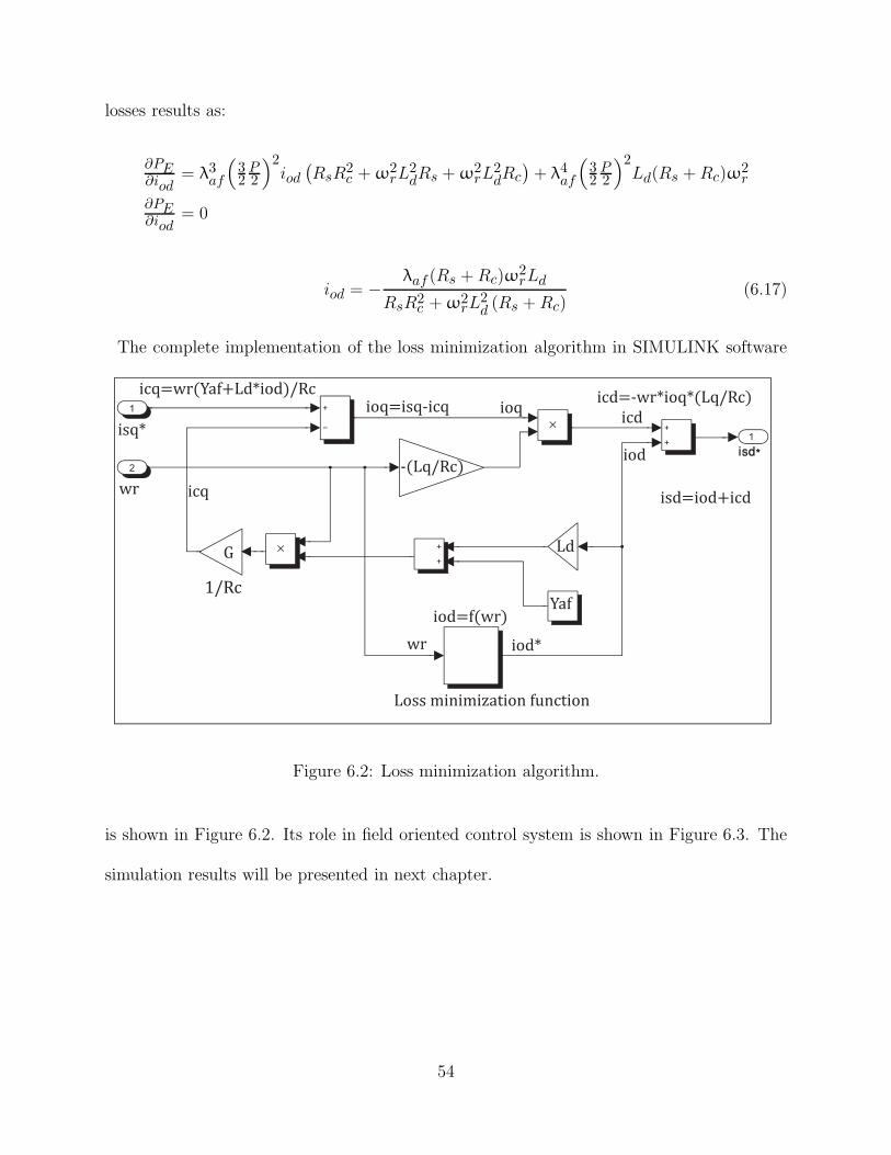
The complete implementation of the loss minimization algorithm in SIMULINK software
ioq=isq-icq ioq
wr
isq*
icq
icq=wr(Yaf+Ld*iod)/Rc
1/Rc
Loss minimization function
wr iod*
iod=f(wr)
iod
icd=-wr*ioq*(Lq/Rc)
icd
isd=iod+icd
isd*
Yaf
Ld
-(Lq/Rc)
G
Figure 6.2: Loss minimization algorithm.
is shown in Figure 6.2. Its role in field oriented control system is shown in Figure 6.3. The
simulation results will be presented in next chapter.
54
Σ Σ
Σ
- -
-
θr
+ +
+
α, β
α, β
α, β
d, q
d, q
v∗sα
v∗sβ
isα
isβ
vr∗qs
vr∗ds
irqs
irds
dθrdt
PI
PIPI
PARK
TRANSFORMATION
TRANSFORMATION
CLARKE
TRANSFORMATION
ir∗qs
SPWM3-PHASE
INVERTER
INV.PARK
PMSM
isa
isb
Vdc
ω∗r
ωr
a, b
ir∗ds
Loss
MinimizationAlgorithm
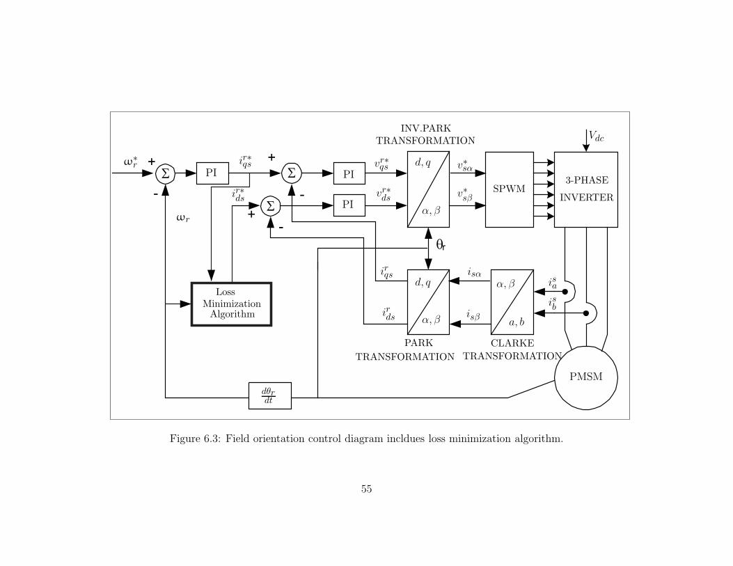
Figure 6.3: Field orientation control diagram incldues loss minimization algorithm.
55
Chapter 7
Simulation Results and Discussion
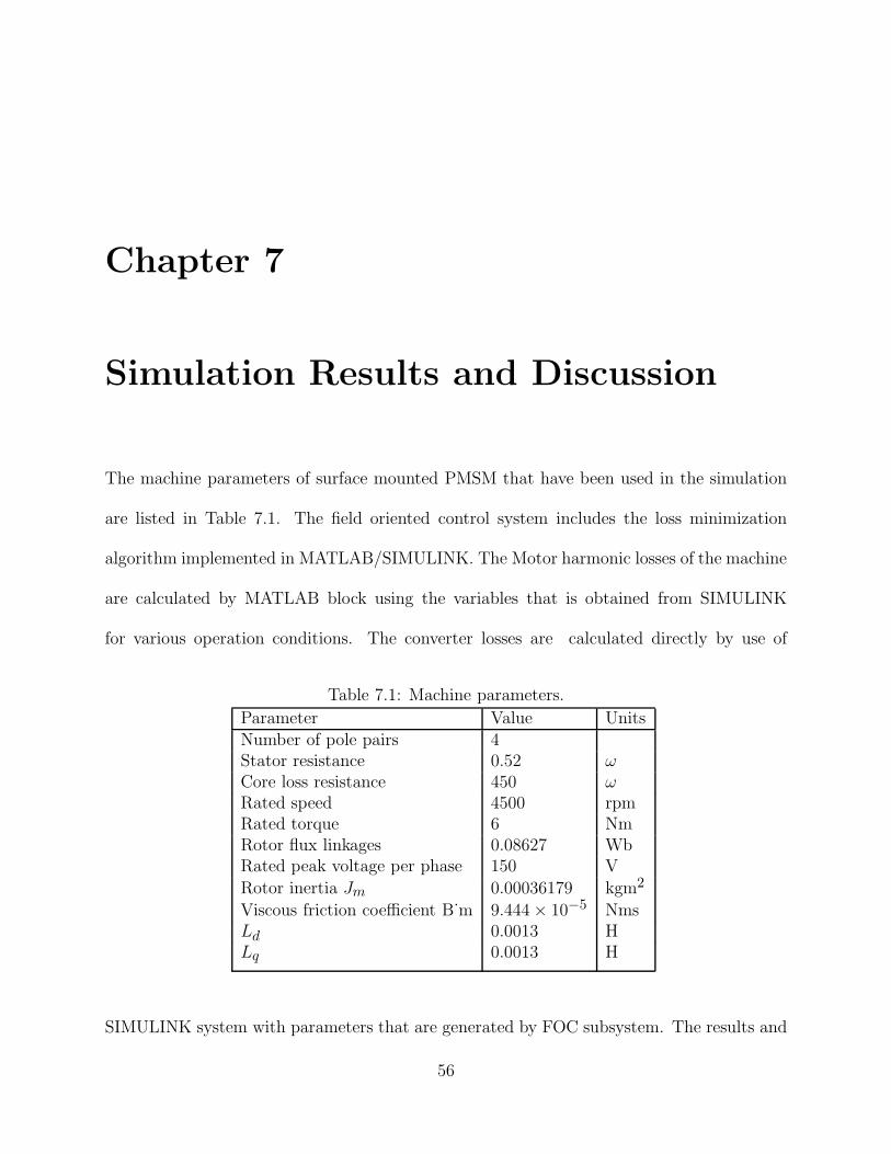
The machine parameters of surface mounted PMSM that have been used in the simulation
are listed in Table 7.1. The field oriented control system includes the loss minimization
algorithm implemented in MATLAB/SIMULINK. The Motor harmonic losses of the machine
are calculated by MATLAB block using the variables that is obtained from SIMULINK
for various operation conditions. The converter losses are calculated directly by use of
Table 7.1: Machine parameters.
Parameter Value UnitsNumber of pole pairs 4Stator resistance 0.52 ω
Core loss resistance 450 ω
Rated speed 4500 rpmRated torque 6 NmRotor flux linkages 0.08627 WbRated peak voltage per phase 150 V
Rotor inertia Jm 0.00036179 kgm2
Viscous friction coefficient B˙m 9.444× 10⁻⁵ NmsLd 0.0013 HLq 0.0013 H
SIMULINK system with parameters that are generated by FOC subsystem. The results and
56
discussion are presented in three sections; FOC under loss minimization control strategy
(LMCS), VSI-motor fundamental losses, and VSI-motor harmonic losses.
7.1 FOC with Loss Minimization Control
The dynamic responses of currents, speed and torque at rated conditions are shown in Figures
7.1 and 7.2, respectively. The system reaches the steady state with smooth dynamic response
in approximate 0.14 second for the system parameters listed in Table 7.1. The current and
speed controllers are designed by a symmetric optimum approach which is addressed in [28].
For calculation of the core loss resistance, it is required that the motor runs at rated speed
and torque of sinusoidal power supply such that the harmonic losses are not generated. The
fundamental iron loss PFe is calculated by subtracting the mechanical and copper losses from
the total output power. The iron loss resistance, Rc, can be obtained from fundamental core
losses as in equation (6.11), where the measured Rc represents the iron loss resistance at the
rated output power. Practically Rc depends on operating conditions. However, it is assumed
constant in this work.
Figure 7.3 shows the efficiency of surface mounted PMSM versus speed for the two control
strategies: zero id control strategy and (LMC) strategy. It is clear that the motor efficiency
under maximum efficiency control strategy is higher than the efficiency under zero id control
strategy. However, the difference in efficiency is not as remarkable for surface mounted
PMSM as for interior PMSM due to the following reasons. In interior PMSM The negative
d-axis current produces a positive reluctance torque due to the saliency (Ld < Lq), and
accordingly the stator current and the copper loss PCu is smaller compared with the id = 0
control. Moreover, in both types of PMSMs the negative d-axis current reduces the flux
57
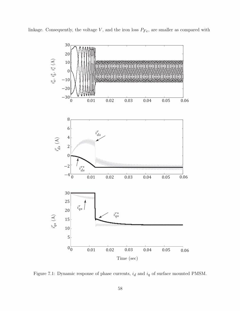
linkage. Consequently, the voltage V , and the iron loss PFe, are smaller as compared with
−2
0
2
4
6
8
0 0.01 0.02 0.03 0.04 0.05 0.06−30
−20
−10
0
10
20
30
0−4
0.01 0.02 0.03 0.04 0.05 0.06
30
0.0600
5
10
15
20
25
0.01 0.02 0.03 0.04 0.05
ir qs(A
)ir ds(A
)is a,is b,is c
(A)
Time (sec)
irds
ir∗ds
ir∗qs
irqs
Figure 7.1: Dynamic response of phase currents, id and iq of surface mounted PMSM.
58
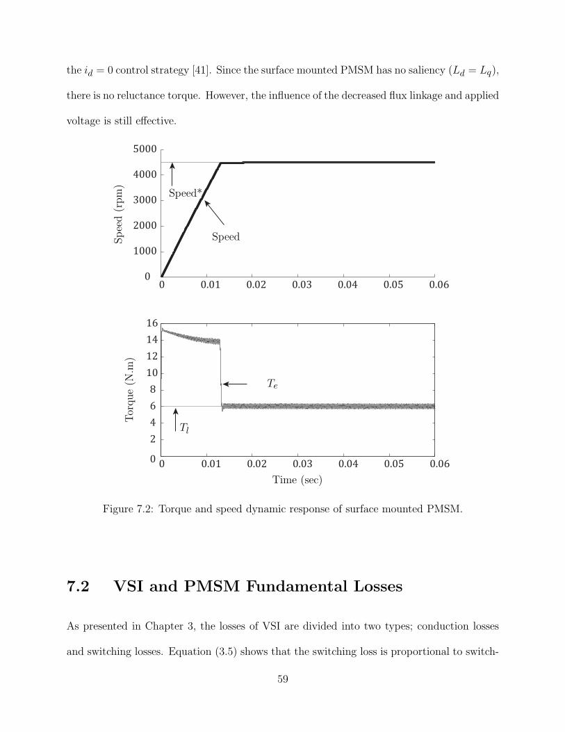
the id = 0 control strategy [41]. Since the surface mounted PMSM has no saliency (Ld = Lq),
there is no reluctance torque. However, the influence of the decreased flux linkage and applied
voltage is still effective.
0 0.01 0.02 0.03 0.04 0.05 0.060
1000
2000
3000
4000
5000
0 0.01 0.02 0.03 0.04 0.05 0.060
2
4
6
8
10
12
14
16
Speed(rpm)
Torque(N
.m)
Time (sec)
Speed
Speed*
Te
Tl
Figure 7.2: Torque and speed dynamic response of surface mounted PMSM.
7.2 VSI and PMSM Fundamental Losses
As presented in Chapter 3, the losses of VSI are divided into two types; conduction losses
and switching losses. Equation (3.5) shows that the switching loss is proportional to switch-
59
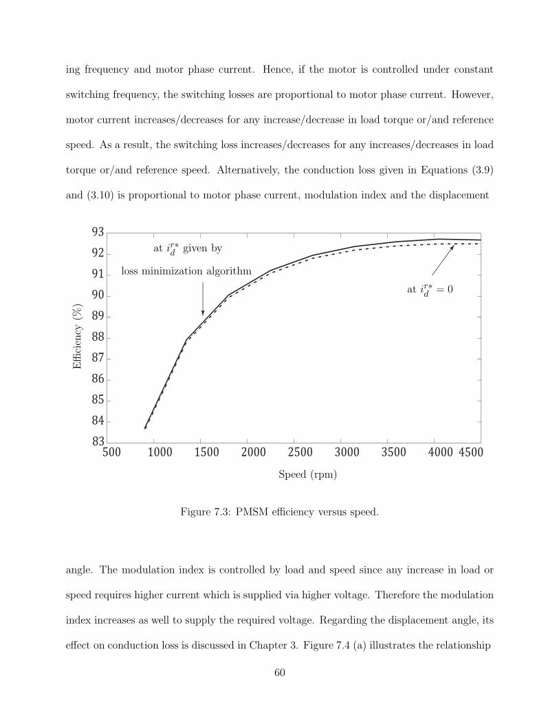
ing frequency and motor phase current. Hence, if the motor is controlled under constant
switching frequency, the switching losses are proportional to motor phase current. However,
motor current increases/decreases for any increase/decrease in load torque or/and reference
speed. As a result, the switching loss increases/decreases for any increases/decreases in load
torque or/and reference speed. Alternatively, the conduction loss given in Equations (3.9)
and (3.10) is proportional to motor phase current, modulation index and the displacement
500 1000 1500 2000 2500 3000 3500 400083
84
85
86
87
88
89
90
91
92
93
4500
Speed (rpm)
Efficiency
(%)
at ir∗d = 0
at ir∗d given by
loss minimization algorithm
Figure 7.3: PMSM efficiency versus speed.
angle. The modulation index is controlled by load and speed since any increase in load or
speed requires higher current which is supplied via higher voltage. Therefore the modulation
index increases as well to supply the required voltage. Regarding the displacement angle, its
effect on conduction loss is discussed in Chapter 3. Figure 7.4 (a) illustrates the relationship
60
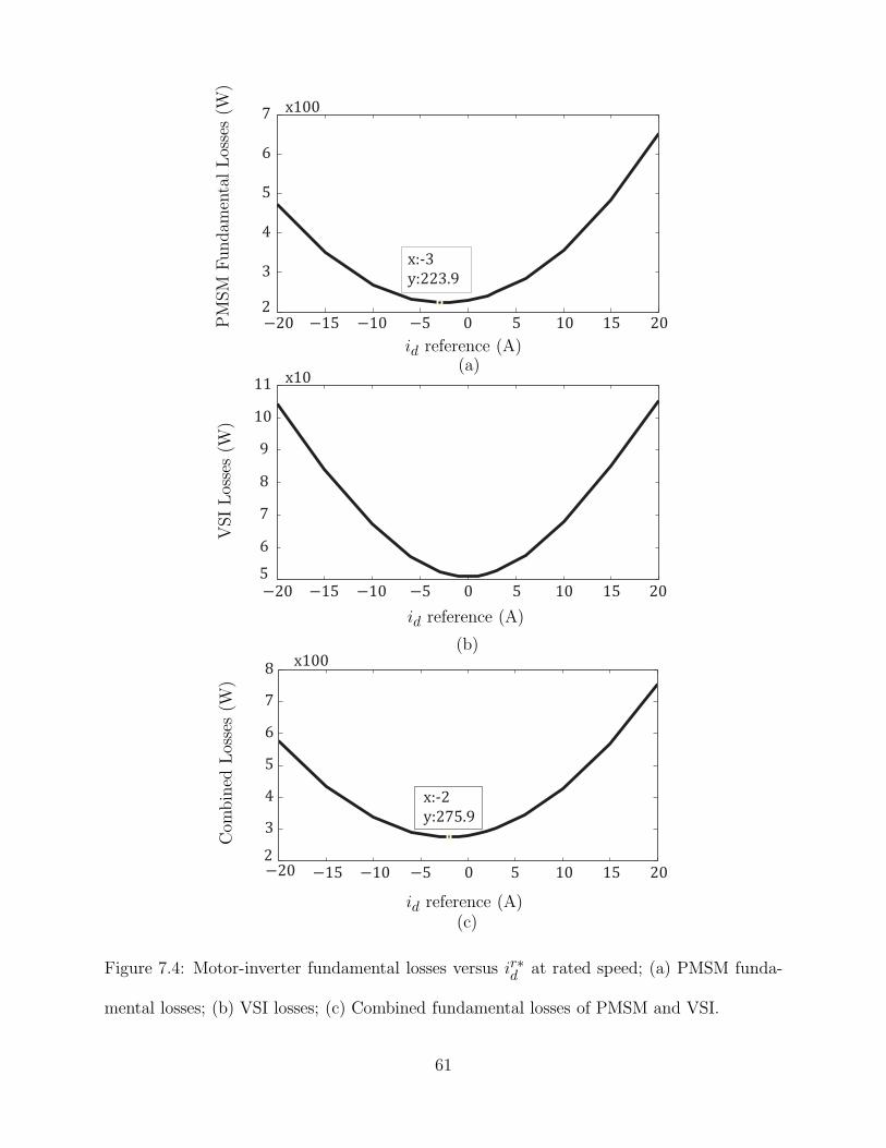
−20 −15 −10 −5 0 5 10 15 20
3
4
5
6
7
−20 −15 −10 −5 0 5 10 15 205
6
7
8
9
10
11
−20 −15 −10 −5 0 5 10 15 202
3
4
5
6
7
8x100
x10
x100
x:-3
y:223.9
x:-2
y:275.9
2
id reference (A)
id reference (A)
id reference (A)
PMSM
Fundam
entalLosses(W
)VSILosses(W
)Com
bined
Losses(W
)
(a)
(b)
(c)
Figure 7.4: Motor-inverter fundamental losses versus ir∗d at rated speed; (a) PMSM funda-
mental losses; (b) VSI losses; (c) Combined fundamental losses of PMSM and VSI.
61
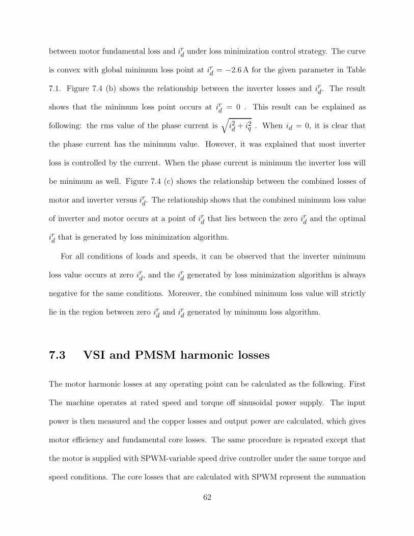
between motor fundamental loss and ird under loss minimization control strategy. The curve
is convex with global minimum loss point at ird = −2.6A for the given parameter in Table
7.1. Figure 7.4 (b) shows the relationship between the inverter losses and ird. The result
shows that the minimum loss point occurs at ird = 0 . This result can be explained as
following: the rms value of the phase current is√
i2d+ i2q . When id = 0, it is clear that
the phase current has the minimum value. However, it was explained that most inverter
loss is controlled by the current. When the phase current is minimum the inverter loss will
be minimum as well. Figure 7.4 (c) shows the relationship between the combined losses of
motor and inverter versus ird. The relationship shows that the combined minimum loss value
of inverter and motor occurs at a point of ird that lies between the zero ird and the optimal
ird that is generated by loss minimization algorithm.
For all conditions of loads and speeds, it can be observed that the inverter minimum
loss value occurs at zero ird, and the ird generated by loss minimization algorithm is always
negative for the same conditions. Moreover, the combined minimum loss value will strictly
lie in the region between zero ird and ird generated by minimum loss algorithm.
7.3 VSI and PMSM harmonic losses
The motor harmonic losses at any operating point can be calculated as the following. First
The machine operates at rated speed and torque off sinusoidal power supply. The input
power is then measured and the copper losses and output power are calculated, which gives
motor efficiency and fundamental core losses. The same procedure is repeated except that
the motor is supplied with SPWM-variable speed drive controller under the same torque and
speed conditions. The core losses that are calculated with SPWM represent the summation
62
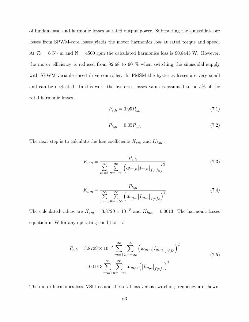
of fundamental and harmonic losses at rated output power. Subtracting the sinusoidal-core
losses from SPWM-core losses yields the motor harmonics loss at rated torque and speed.
At Te = 6 N · m and N = 4500 rpm the calculated harmonics loss is 90.8445 W. However,
the motor efficiency is reduced from 92.68 to 90 % when switching the sinusoidal supply
with SPWM-variable speed drive controller. In PMSM the hysterics losses are very small
and can be neglected. In this work the hysterics losses value is assumed to be 5% of the
total harmonic losses.
Pe,h = 0.95Pc,h (7.1)
Ph,h = 0.05Pc,h (7.2)
The next step is to calculate the loss coefficients Kem and Khm :
Kem =Pe,h
∞∑
m=1
∞∑
n=−∞
(
ωm,n
∣
∣Im,n
∣
∣
f 6=f◦
)2(7.3)
Khm =Ph,h
∞∑
m=1
∞∑
n=−∞
(
ωm,n
∣
∣Im,n
∣
∣
f 6=f◦
)2(7.4)
The calculated values are Kem = 3.8729 × 10⁻⁸ and Khm = 0.0013. The harmonic losses
equation in W for any operating condition is:
(7.5)
Pc,h = 3.8729× 10⁻⁸∞∑
m=1
∞∑
n=−∞
(
ωm,n
∣
∣Im,n
∣
∣
f 6=f◦
)2
+ 0.0013
∞∑
m=1
∞∑
n=−∞ωm,n
(
∣
∣Im,n
∣
∣
f 6=f◦
)2
The motor harmonics loss, VSI loss and the total loss versus switching frequency are shown
63
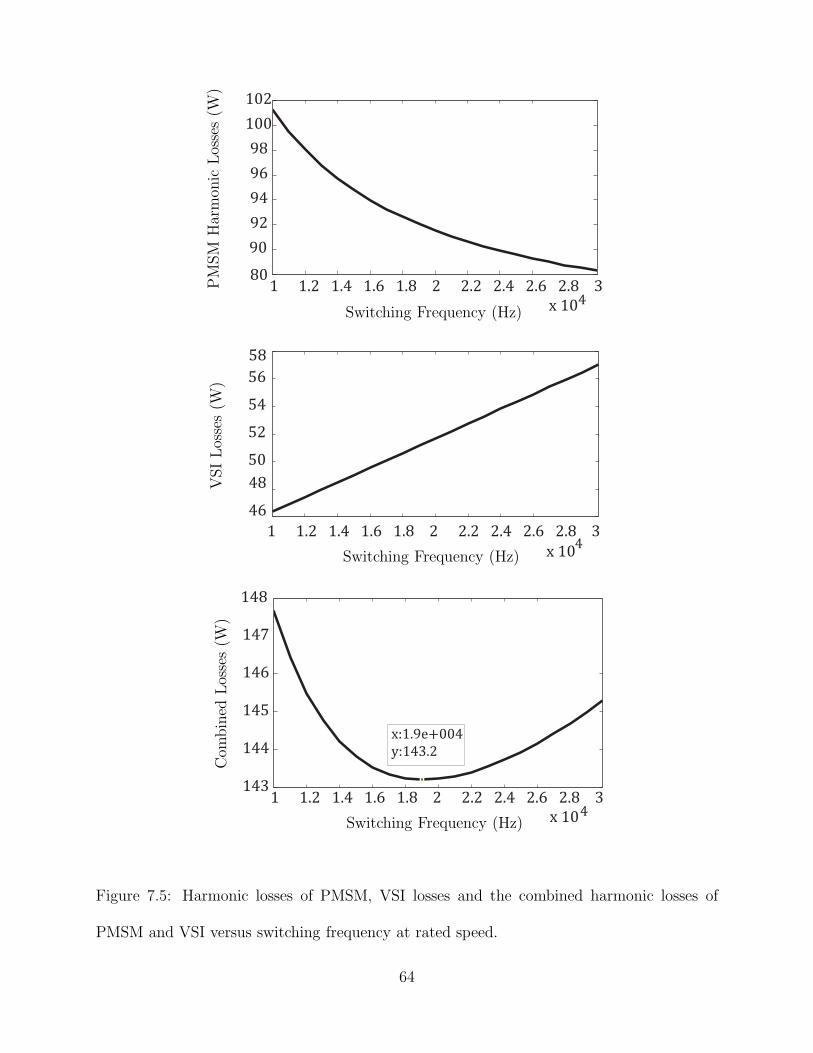
50
52
54
56
58
90
92
94
96
98
100
102
80
143
144
145
146
147
x:1.9e+004
y:143.2
148
1 1.2 1.4 1.6 1.8 2 2.2 2.4 2.6 2.8 3
x 10
1 1.2 1.4 1.6 1.8 2 2.2 2.4 2.6 2.8 3
x 10
1 1.2 1.4 1.6 1.8 2 2.2 2.4 2.6 2.8 3
x 10
46
48
4
4
4
Switching Frequency (Hz)
Switching Frequency (Hz)
Switching Frequency (Hz)
PMSM
Harmon
icLosses(W
)VSILosses(W
)Com
bined
Losses(W
)
Figure 7.5: Harmonic losses of PMSM, VSI losses and the combined harmonic losses of
PMSM and VSI versus switching frequency at rated speed.
64
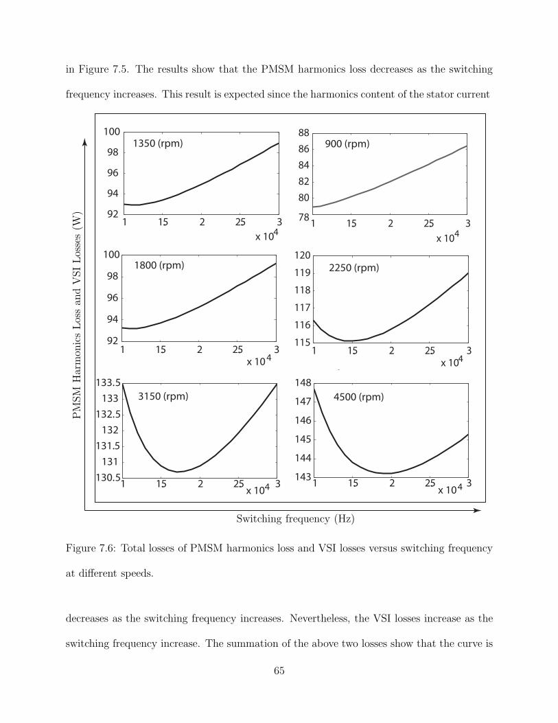
in Figure 7.5. The results show that the PMSM harmonics loss decreases as the switching
frequency increases. This result is expected since the harmonics content of the stator current
1 1.5 2 2.5 3130.5
131
131.5
132
132.5
133
133.5
1 1.5 2 2.5 3143
144
145
146
147
148
1 1.5 2 2.5 3x 10⁴
115
116
117
118
119
120
1 1.5 2 2.5 3x 10⁴
92
94
96
98
100
1 1.5 2 2.5 3
x 104
92
94
96
98
100
1 1.5 2 2.5 3
x 104
78
80
82
84
86
88
x 10 x 104 4
1350 (rpm) 900 (rpm)
1800 (rpm) 2250 (rpm)
3150 (rpm) 4500 (rpm)
Switching frequency (Hz)
PMSM
Harmon
icsLossan
dVSILosses(W
)
Figure 7.6: Total losses of PMSM harmonics loss and VSI losses versus switching frequency
at different speeds.
decreases as the switching frequency increases. Nevertheless, the VSI losses increase as the
switching frequency increase. The summation of the above two losses show that the curve is
65
convex and has global minimum loss value at the switching frequency of 19 kHz. However
the specific optimal switching frequency will depend on particular set of design parameters
of the VSI. In other words, when the parameters of the VSI such that the loss of VSI higher
than the motor harmonics loss at the same range of switching frequency, the curve will be
no more convex and almost will be linear.
0 0.1 0.2 0.3 0.4 0.5 0.6 0.7 0.8 0.9 10
20
40
60
80
100
120
X=0.73
Y=112.2
Modulation Index
PMSM
Harmon
icsLoss(W
)
Figure 7.7: PMSM harmonics loss versus modulation index.
Figure 7.6 shows the combined loss of motor harmonics loss and VSI loss versus switching
frequency at different speeds and rated torque. The result shows that the total losses increase
as the motor speed increases. Also, at low speeds up to 50 % of the rated speed the VSI
loss is dominant. When the speed increases, the motor harmonic losses become dominant
such that the loss curve becomes convex. Figure 7.7 shows the relationship between PMSM
harmonic loss and modulation index. It can be seen that up to M = 0.73 the harmonics loss
increases as the modulation index increases. As the modulation index passes M = 0.73, the
66
harmonics loss begins to decrease to locally minimum loss value at unity modulation index.
Because the loss is minimum near unity modulation index, it is suitable to use variable dc
link such that the modulation index is kept near the unity at all loads and speeds.
7.4 Conclusions
The main results of the thesis work can be summarized in the following aspects:
• The motor loss that is caused by the fundamental component of phase currents can
be minimized by using the maximum efficiency control strategy with the assumption
that the core loss resistance and copper loss resistance are constant under all operating
conditions.
• The combined motor-inverter fundamental losses are minimized under maximum effi-
ciency control strategy in the region in which ir∗d < id < 0.
• PMSM harmonics loss can be minimized by increasing the converter switching fre-
quency with the assumption that SPWM inverter is used without any harmonics in-
jection technique.
• For a given range of switching frequencies in which the motor can work with acceptable
performance, the choice of minimal switching frequency would minimize the converter
loss.
• For a given range of switching frequencies in which the motor can deliver acceptable
performance, the choice of the optimum switching frequency that will minimize motor-
inverter losses follows the parametric optimization. The optimal loss point is affected
67

by the system parameters. Hence, changing of the values of VSI parameters would
vary the optimal point of motor-inverter losses.
7.5 Recommendations for Future work
In the thesis work it has been assumed that Rc, Khm, and Khm are constants. Practically,
the core losses of the machine are not constant due to the variations in the properties of
magnetic material. Modeling the core losses at rated condition may yield inaccurate results
in variable speed drive machine. The expected future work is taking into account the change
in laminations properties due to operating condions while modeling core losses. However, it
is planned to verify the harmonic loss model by using real time controller.
68

BIBLIOGRAPHY
69
BIBLIOGRAPHY
[1] G. Slemon, “High-efficiency drives using permanent-magnet motors,” IECON Proceed-ings, pp. 725–730, 1993.
[2] M. Rahman, “High efficiency permanent magnet synchronous motors,” IEEE IAS Meet-ing, pp. 561–564, 1979.
[3] P. Pillay and R. Krishnan, “Application characteristics of pm synchronous and bdcmmotor servo drives,” Conf. Record, IEEE IAS Annual Meeting, Atlanta, pp. 380–390,Oct. 1987.
[4] G. Slemon and X. Liu, “Core losses in permanent magnet motors,” IEEE Transactionson Magnetics, vol. 26, no. 5, pp. 1653–1656, Sep. 1990.
[5] R. Colby and D. Novotny, “Efficient operation of pm synchronous motors,” IEEE Trans-actions on Industry Applications, vol. IA-23, pp. 1048–1054, Nov./Dec. 1987.
[6] T. H. S. Morimoto, Y. Tong, “Loss minimization control of permanent magnet syn-chronous motor drives,” Transactions on Industry Applications, vol. 41, no. 5, pp. 511–517, Oct. 1994.
[7] R. Schiferl and T. Lipo, “Core losses in buried magnet permanent magnet synchronousmotors,” IEEE Transactions On Energy Conversion, vol. 4, no. 2, pp. 279–284, June1989.
[8] T. L. D. N. L. Xu, X. Xu, “Vector control of a synchronous reluctance motor includingsaturation and iron loss,” IEEE Transactions on Industry Applications, vol. 27, no. 5,pp. 978–985, Sep./Oct. 1991.
70
[9] T. G. J. Flecher, B. Williams, “Efficiency aspects of vector control applied to syn-chronous reluctance motors,” Conference Proceedings, IEEE IAS meeting, pp. 294–300,1995.
[10] R. F. F. Fernandez-Bernal, A. Garcia, “Efficient control of reluctance synchronous ma-chines,” IEEE IECON, pp. 923–928, 1998.
[11] Y. K. K. J. J. Lee and H. Nam, “Loss distribution of three-phase induction motor fed bypulsewidth-modulated inverter,” IEEE Trans.Magn., vol. 40, no. 2, pp. 762–765, Mar.2004.
[12] E. N. Hildebrand and H. Roehrdanz, “Losses in three-phase induction machines fed bypwm converter,” IEEE Trans. Energy Convers., vol. 16, no. 3, pp. 228–233, Sep. 2001.
[13] A. J. M. P. J. Leonard, P. Marketos and M. Lu, “Iron losses under pwmexcitation usinga dynamic hysteresis model and finite elements,” IEEE Trans. Magn., vol. 42, no. 4,pp. 907–910, Apr. 2007.
[14] T. H. Kim and J. Lee, “Comparison of the iron loss of a flux-reversal machine underfour different pwm modes,” IEEE Trans. Magn., vol. 43, no. 4, pp. 1725–1728, Apr.2007.
[15] K. S. H. Toda and M. Ishida, “Effect of material properties on motor iron loss in pmbrushless dc motor,” IEEE Trans. Magn., vol. 41, no. 10, pp. 3937–3939, Oct. 2005.
[16] A. J. M. J. Sagarduy and F. J. Anayi, “Current losses in electrical steels subjected tomatrix and classical pwm excitation waveforms,” IEEE Trans. Magn., vol. 42, no. 10,pp. 2818–2820, Oct. 2006.
[17] K. Yamazaki and Y. Seto, “Iron loss analysis of interior permanent- magnet synchronousmotors-variation of main loss factors due to driving condition,” IEEE Trans. Ind. Appl.,vol. 42, no. 4, pp. 1045–1052, Jul./Aug. 2006.
[18] T. L. M. A. Boglietti, A. Cavagnino and P. Pillay, “Comparison of lamination iron lossessupplied by pwm voltages: Us and european experiences,” in Proc. IEEE Int. Electr.Machines Drives Conf., pp. 1431–1436, May 2005.
[19] M. L. A. Boglietti, P. Ferraris and M. Pastorelli, “Change of the iron losses with theswitching supply frequency in soft magnetic materials supplied by pwm inverter,” IEEETrans. Magn., vol. 31, no. 6, pp. 4250–4252, Nov. 1995.
71
[20] M. L. A. Boglietti, P. Ferraris and F. Profumo, “effects of different modulation indexon the iron losses in soft magnetic materials supplied by pwm inverter,” IEEE Trans.Magn., vol. 29, no. 6, pp. 3234–3236, Nov 1993.
[21] M. P. P. T. Lotten and N. A. Singampalli, “Lamination core loss measurements inmachines operating with pwm or non-sinusoidal excitation,” in Proc. Electr. MachinesDrives Conf., vol. 2, pp. 743–746, Jun. 1-4 2003.
[22] L. M. F. Sixdenier and J. P. Masson, “Introducing dynamic behavior of magnetic ma-terials into a model of a switched reluctance motor drive,” IEEE Trans. Magn., vol. 42,no. 3, pp. 398–404, Mar. 2006.
[23] A. Ruderman, “Electrical machine pwm loss evaluation basics,” in Energy Efficiency inMotor Driven Systems, Heidelberg, Germany, Sep., 5-8 2005.
[24] M. K. Jamil and N. A. Demerdash, “Harmonics and core losses of permanent magnetdc motors controlled by chopper circuits,” IEEE Trans. Energy Convers., vol. 5, no. 2,pp. 408–414, Jun. 1990.
[25] M. K. Jamil and N. Demerdash, “Effects of chopper control circuits on core losses ofpermanent magnet dc motors,” IEEE Trans. Magn., vol. 25, no. 5, pp. 3572–3574, Sep1989.
[26] M. L. A. Boglietti, P. Ferraris and M. Pastorelli, “About the possibility of defining astandard method for iron loss measurement in soft magnetic materials with invertersupply,” IEEE Trans. Ind. Appl., vol. 33, no. 5, pp. 1283–1288, Sep 1997.
[27] C. G. D. Ruifang Liu, Mi, “Modeling of eddy-current loss of electrical machines andtransformers operated by pulsewidth-modulated inverters,” IEEE Transactions on Mag-netics, vol. 44, no. 8, pp. 2021–2028, Aug. 2008.
[28] R. Krishnan, “Permanent magnet synchronous and brushless dc motor drives,” Taylorand Francis Group, LLC, 2010.
[29] H. D. Zhu, Z.Q., “Instantaneous magnetic field distribution in brushless permanent mag-net dc motors. ii. armature-reaction field,” IEEE Transactions on Magnetics, vol. 29,no. 1, pp. 136–142, Jan. 1993.
[30] B. Holmes, D.G.; McGrath, “Opportunities for harmonic cancellation with carrier basedpwm for two-level and multi-level cascaded inverters,” Industry Applications Conference,
72
1999. Thirty-Fourth IAS Annual Meeting. Conference Record of the 1999 IEEE, vol. 2,pp. 781–788, 1999.
[31] M. Bierhoff and F. Fuchs, “Semiconductor losses in voltage source and current sourceigbt converters based on analytical derivation,” in Proc. Power Electronics Specialistsconference (PESC 04), vol. 4, pp. 2836–2842, 2004.
[32] U. Nicolai, T. Reimann, J. Petzoldt, and J. Lutz, “Semikron,applikationshandbuch igbt-und mosfet-leistungsmodule,” ISLE, 1998.
[33] F. Casanellas, “Losses in pwm inverters using igbts,” IEE Proc. Electr. Power Appl.,vol. 141, no. 5, pp. 235–239, Sep. 1994.
[34] L. Mestha and P. Evans, “Analysis of on-state losses in pwm inverters,” IEE Proceedings,vol. 136, no. 4, July 1989.
[35] D. Chung and S. Sul, “Minimum-loss pwm strategy for 3-phase pwm rectifier,” PESC,vol. 2, pp. 1020–1027, 1997.
[36] K. Zhou and D. Wang, “Relationship between space-vector modulation and three-phasecarrier-based pwm: A comprehensive analysis,” IEEE Trans. on Ind. Electr., vol. 49,no. 1, pp. 186–196, February 2002.
[37] K. R. PILLAY, P., “Modeling of permanent magnet motor drives,” IEEE TRAN. onIndustrial Electronics, vol. 35, no. 4, Nov. 1988.
[38] T. Instruments, “Field orientated control of 3-phase ac-motors,” Texas InstrumentsEurope, Literature Number: BPRA073, Feb. 1998.
[39] S. T. Pekarek, S., “Acsl/graphic modeller component models for electric power educa-tion,” IEEE Tran. on Education, vol. 41, no. 4, Nov. 1998.
[40] U. M. R. P. Moham, N., “Power electronics converters applications and design,” JohnWiley and Sons, INC., second edition, 1995.
[41] T. Y. T. Y. H. T. Morimoto, S., “Loss minimization control of permanent magnetsynchronous motor drives,” IEEE TRAN. on industrial Electronics, vol. 41, no. 5, pp.511–517, Oct 1994.
73
![[MoD3-5]Efficiency Optimization of PMSM Based Drive Systembingsen/files_publications/C-12_IPEMC_2.pdf · Emails: hassanwa@msu.edu; bingsen@egr.msu.edu Abstract—The proposed work](https://img.pdfslide.net/doc/110x75/5e51772b22eaea142a4f8793/mod3-5efficiency-optimization-of-pmsm-based-drive-system-bingsenfilespublicationsc-12ipemc2pdf.jpg)