Embed Size (px)
Citation preview

JOURNAL OF ALGORJTHMS 5, 80-131 (1984)
Efficient Algorithms for a Family of Matroid Intersection Problems*
HAROLDN.GABOW+
Department of Computer Science, Universiy of Colorado, Boulder, Colorado 80309
AND
ROBERT E. TARJAN*
Computer Science Department, Stanford iJniversi@, Stanjorcl, Califotnia 94305
Received April 9.1982
Consider a matroid where each element has a real-valued cost and a color, red or green; a base is sought that contains q red elements and has smallest possible cost. An algorithm for the problem on general matroids is presented, along with a number of variations. Its efficiency is demonstrated by implementations on specific matroids. In all cases but one, the running time matches the best-known algorithm for the problem without the red element constraint: On graphic matroids, a smallest spanning tree with q red edges can be found in time O(nlog n) more than what is needed to find a minimum spanning tree. A special case is finding a smallest spanning tree with a degree constraint; here the time is only O(m + n) more than that needed to find one minimum spanning tree. On transversal and matching matroids, the time is the same as the best-known algorithms for a minimum cost base. This also holds for transversal matroids for convex graphs, which model a scheduling problem on unit-length jobs with release times and deadlines. On partition matroids, a linear-time algorithm is presented. Finally an algorithm related to our general approach finds a smallest spanning tree on a directed graph, where the given root has a degree constraint. Again the time matches the best-known algorithm for the problem without the red element (i.e., degree) constraint.
*A preliminary version of this paper appeared in the Proceedings of the 20th Annual Symposium on the Foundations of Computer Science, San Juan, Puerto Rico [GTl].
+The work of this author was supported in part by the National Science Foundation under Grant MCS 78-18909.
*Current address: AT&T, Bell Laboratories, Murray Hill, N.J. 07974. The work of this author was supported in part by the National Science Foundation under Grant MCS75-22870, by the Office of Naval Research, Contract N 00014-76-C-0688, and by a Guggenheim Fellowship.
01%~6774/84 $3.00 Copyright 0 1984 by Academic Press. Inc. . . . .~L_~ ~c- ~> _. *
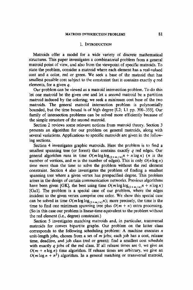
MATROIDINTERSECTIONPROBLEMS 81
1. INTRODUCTION
Matroids offer a model for a wide variety of discrete mathematical structures. This paper investigates a combinatorial problem from a general matroid point of view, and also from the viewpoint of specific matroids. To state the problem, consider a matroid where each element has a real-valued cost and a color, red or green. We seek a base of the matroid that has smallest possible cost subject to the constraint that it contains exactly q red elements, for a given q.
Our problem can be viewed as a matroid intersection problem. To do this let one matroid be the given one and let a second matroid be a partition matroid induced by the coloring; we seek a minimum cost base of the two matroids. The general matroid intersection problem is polynomially bounded, but the time bound is of high degree [L2; Ll pp. 300-3551. Our family of intersection problems can be solved more efficiently because of the simple structure of the second matroid.
Section 2 reviews some relevant notions from matroid theory. Section 3 presents an algorithm for our problem on general matroids, along with several variations. Applications to specific matroids are given in the follow- ing sections.
Section 4 investigates graphic matroids. Here the problem is to find a smallest sparming tree (or forest) that contains exactly q red edges. Our general algorithm runs in time O(m loglogC,+,,,,n + n log n) (n is the number of vertices, and m is the number of edges). This is only 0( n log n) time more than the time to solve the problem without the red element constraint. Section 4 also investigates the problem of finding a smallest spanning tree where a given vertex has prespecified degree. This problem arises in the design of certain communication networks. Previous algorithms have been given [GK], the best using time O(mloglog(,+,,,,n + n log n) [Gal]. The problem is a special case of our problem, where the edges incident to the given vertex comprise one color. We show this special case can be solved in time O(mloglogC,+,,,, n); more precisely, the time is the time to find one minimum spanning tree plus O(m + n) extra processing. (So in this case our problem is linear-time equivalent to the problem without the red element (i.e., degree) constraint.)
Section 5 investigates matching matroids and, in particular, transversal matroids for convex bipartite graphs. Our problem on the latter class corresponds to the following scheduling problem: A machine executes n unit-length jobs, chosen from a set of m jobs; each job has a cost, release time, deadline, and job class (red or green); find a smallest cost schedule with exactly q jobs of the red class. If all release times are 0, we give an 0( m + n log n) time algorithm. If release times are arbitrary, we give an 0( m log n + n*) algorithm. In a general matching or transversal matroid,
82 GABOW AND TARJAN
we give an O(m log m + ne) time algorithm (here m is the number of vertices of the graph, n is the number of edges in a maximum matching (thus n G m), and e is the number of edges in the graph). In all cases our time bound equals the best-known bound for finding a minimum cost base of the matroid without the red element constraint.
Section 6 investigates partition matroids. Here the problem is, given a set with a partition, where each element has a cost and color, find a smallest subset containing exactly ni elements from the i th block of the partition, and exactly q red elements. We give a linear-time (and hence optimal) algorithm for this problem.
Section 7 discusses the problem of finding a smallest directed spanning tree with a prespecified root, where the root has a prespecified degree. This is closely related to our matroid intersection problem. However, since the solution is a base of three matroids rather than two, the general theory does not apply. We present an Omin(m log n, n*) algorithm. Again this bound matches the best-known algorithm for the problem without the degree constraint.
For the algorithms that are not optimal we give a weak type of lower bound: We show that any algorithm using an approach similar to ours, “the swap sequence approach,” has a nonlinear lower bound. In some cases this bound matches our upper bound.
All of our algorithms easily generalize to the problem where the desired base contains at most (or at least) q red elements. Thus this paper gives evidence that a “q red elements” constraint can often be handled efficiently.
2. MATROID PRELIMINARIES
This section reviews some basic facts about matroids. It is assumed that the reader is familiar with an introductory treatment of matroids, such as
6 4
FIG. 2.1. Graphic matroid with colors and edge costs.

MATROID INTERSECTION PROBLEMS 83
I 0 Bo 6Fw; -9+46G-‘3+6
83 = Bp-zt3 84’83~1+5
FIG. 2.2. Optimum bases and swap sequence.
[Ll, Ch. 71 or [W, Ch. 11. Our terminology comes mainly from the former. Definitions of fundamental concepts such as independent set, base, and circuit can be found in these sources.
We use a convenient shorthand notation for set operations: If S is a set andeanelement,thenS+eisthesetSU{e},andS-eisS-{e}.We sometimes use + instead of U, as in B - G + R (for sets B, G, R). When parentheses are omitted, operators are associated to the left, e.g., S + e - f is (S + e) - f. s is the complement of set S.
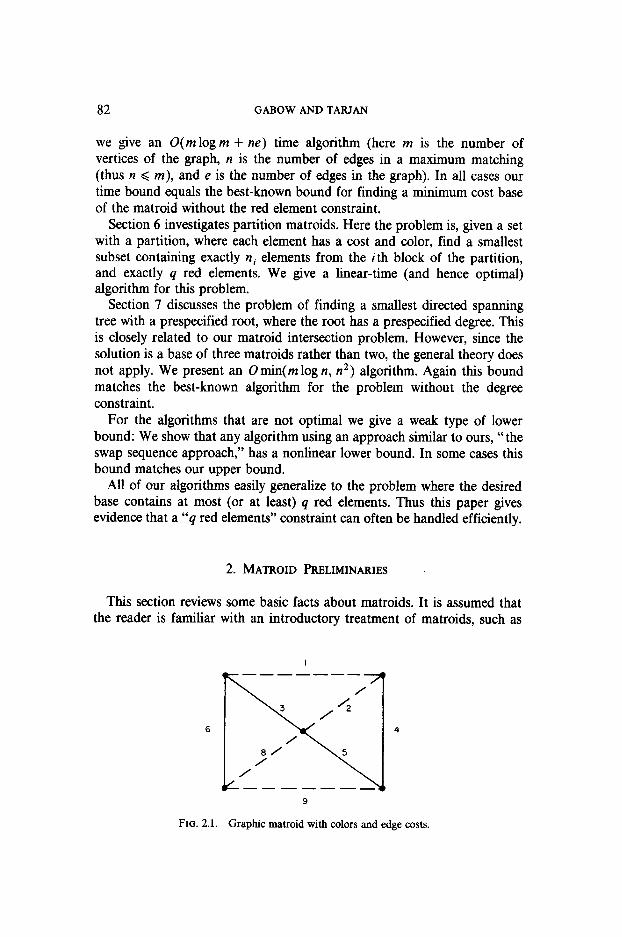
We use graphic matroids to illustrate the discussion on general matroids. A graphic matroid derives from a graph or multigraph.’ The elements of the matroid are the edges of the graph. The independent sets are the forests, and the bases are the spanning forests (or sparming trees, if the graph is connected). Figure 2.1 shows a graph (with solid and dotted edges); Fig. 2.2 gives several bases. (We will give a more precise description of these figures shortly).
Our results follow from one simple property of matroids, which can be included in a set of matroid axioms:
Symmetric Swap Axiom [B; Wp. 151. If B, and B2 are bases and element f E B,, then there is an element e E B2 such that both B, - f + e and B, - e + f are bases.
The Symmetric Swap Axiom is a strong formulation of the more standard base axiom of a matroid [Ll, p. 2741. It can be derived from the indepen-
‘Throughout this paper graphs are undirected unless explicitly specified otherwise. Also when our algorithms work on multigraphs we say so and then proceed to give the discussion in terms of graphs.
84 GABOW AND TARJAN
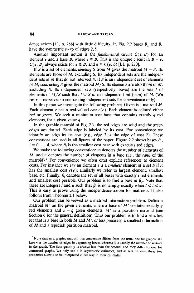
dence axiom [Ll, p. 2681 with little difficulty. In Fig. 2.2 bases B, and B4 have the symmetric swap of edges 2,5.
Another important notion is the fundamental circuit C(e, B) for an element e and a base B, where e @ B. This is the unique circuit in B + e. C(e, B) always exists for e @ B, and e E C(e, b) [Ll, p. 2701.
If S is a set of elements, deleting S from M gives the matroid M - S. Its elements are those of M, excluding S. Its independent sets are the indepen- dent sets of M that do not intersect S. If S is an independent set of elements of M, contracting S gives the matroid M/S. Its elements are also those of M, excluding S. Its independent sets (respectively, bases) are the sets I of elements of M/S such that I u S is an independent set (base) of M. (We restrict ourselves to contracting independent sets for convenience only).
In this paper we investigate the following problem. Given is a matroid M. Each element e has a real-valued cost c(e). Each element is colored either red or green. We seek a minimum cost base that contains exactly q red elements, for a given value q.
In the graphic matroid of Fig. 2.1, the red edges are solid and the green edges are dotted. Each edge is labeled by its cost. For convenience we identify an edge by its cost (e.g., edge 2 is the edge of cost 2). These conventions are used in all figures of the paper. Figure 2.2 shows bases Bi, i=O , . . . ,4, where Bi is the smallest cost base with exactly i red edges.
We make the following convention: m denotes the number of elements of M, and n denotes the number of elements in a base (i.e., the rank of the matroid).2 For convenience we often omit explicit references to element costs. For instance we say an element e is a smallest element of a set S if it has the smallest cost c(e); similarly we refer to largest element, smallest base, etc. Finally, pi denotes the set of all bases with exactly i red elements and smallest cost possible. Our problem is to find a base in p4. Note that there are integers 1 and u such that pi is nonempty exactly when 1~ i G u. This is easy to prove using the independence axiom for matroids. It also follows from Theorem 3.1 below.
Our problem can be viewed as a matroid intersection problem. Define a matroid M’ on the given elements, where a base of M’ contains exactly q red elements and n - q green elements. M’ is a partition matroid (see Section 6 for the general definition). Thus our problem is to find a smallest set that is a base in both M and M’, or less precisely, a smallest intersection of M and a (special) partition matroid.
*Note that in a graphic matroid this convention differs from the usual one for graphs. We take n as the number of edges in a spanning forest, whereas it is usually the number of vertices in the graph. The first quantity is always less than the second, and they differ by one for connected graphs. We only use n in asymptotic estimates, and as will be seen, these two properties allow n to be interpreted either way in these estimates.

MATROIDINTERSECTIONPROBLEMS 85
3. THE GENERAL ALGORITHM
This section presents an algorithm for our intersection problem on arbitrary matroids; useful variations are also given. The efficiency is il- lustrated for the case of graphic matroids. Subsequent sections show that the algorithm and its variants are efficient on other matroids.
The results of this section were discovered independently by Dan Gusfield [Gu]. Gusfield investigates the problem of uniformly modifying the costs of red elements. His derivation is concise and elegant, and contains all the results of this section (either explicitly or implicitly). Here we give our own development (different from Gusfield’s) so the paper is self-contained. (Also, some ideas of this section for the special case of graphic matroids appear in [Gal, U].)
The general matroid intersection problem can be solved by augmenting paths [Ll, pp. 326-3481. In our problem these paths are particularly simple, as we now show.
DEFINITION 3.1. A swap for a base B is an ordered pair of elements (e,f),whereeEBisgreen,f4Bisred,andB-e+fisabase.Thecost of (e, f) is c(f) - c(e).
We say that (e, f ) is a swap for f, for f and B, etc. Following a previous convention, we say (e, f) is a smallest (largest) swap if its cost is as small (large) as possible.
Figure 2.2 shows four swaps executed serially on the matroid of Fig. 2.1. A base Bi E pi derives from Bi _ t E & _ t by a swap. The following result shows this is true in general.
THEOREM 3.1 (Augmentation Theorem). Suppose B is a base in fii _ 1 and Pi f 0. If@, f> is a smallest swap for B, then B - e + f E pi.
ProoJ: It suffices to find a swap (e, f) such that B - e + f E pi. For this implies that (e, f) is a smallest swap for B, and further, any smallest swap for B gives a base in pi. (Also it implies that the swap of the Theorem always exists.)
Choose base B’ E fli such that IB n B’I is maximum. Let f be a red element in B’ - B (f exists since B’ has more red elements than B). By the Symmetric Swap Axiom, there is an element e E B such that B - e + f and B’ - f + e are bases. Clearly e Z f.
We show e is green by contradiction. If e is red then B’ - f + e is a base with i red elements. Thus c( B’ - f + e) >/ c( B’), so c(e) z c( f ). Similarly examining base B - e + f shows c(f) > c(e). We conclude c(e) = c( f ). Thus B’ - f + e is a base in fii having more elements in common with B than B’. This is the desired contradiction.
Now since e is green, B - e + f is a base with i red elements, and B’ - f + e is a base with i - 1 red elements. The latter implies c(B’ - f +

86 GABOWANDTARJcjN
e) 3 c(B), or equivalently c(B’) z c(B - e + f). This inequality shows B - e f f E pi, as desired. 0
Note that this proof is easily modified to show that pi # 0 exactly when 1 d i G U, for two integers 1 and u (see Section 2). (If & P, + 0 for T < s, show &+1 # 0 by starting with B E Is, and choosing B’ E 18, as in the proof .)
The Augmentation Theorem implies an algorithm for our problem: Start with a base in 8,. In general, having derived a base in &, find a smallest swap and derive a base in fli + 1. Repeat this procedure until a base in & is derived.
We improve the efficiency of this approach in several ways. First we show that the elements involved in swaps can be drawn from a restricted set. Recall u is the largest index with & # 0.
COROLLARY 3.1. Let B be a base in &, and B’ a base in &. Then there is a smallest swap (e, f) for B, with e E B - B’ and f E B’ - B.
Proof. Let (g, h) be a smallest swap for B. We first find a smallest swap (g, f) with f E B’ - B. Then we find the desired swap (e, f).
The Symmetric Swap Axiom applied to h, B - g + h, and B’ shows there is an element f E B’ such that B - g + f and B’ - f + h are bases. f is red. For otherwise since h is red, B’ - f + h is a base with u + 1 red elements, which is impossible.
Sincefisred,f#g.SinceB-g+fisabase,wehavefEB’-Band (g, f) is a swap for B. For (g, f) to be a smallest swap we must have c(h) 2 c( f ). To see this, note B’ - f + h has u red elements, so c( B’ - f + h) 3 c( B’), and c(h) 2 c( f ). Thus (g, f) is as desired.
If g GZ B’, then take e = g, and swap (e, f) gives the Corollary. Otherwise find e by applying the Symmetric Swap Axiom to g, B - g + f, and B’. The argument is analogous to the one above and is left to the reader. q
Another useful fact is that swaps get progressively more expensive. Corollary 3.2 is a formulation of this fact that is used in Section 4.2; Corollary 3.3 is another formulation.
COROLLARY 3.2. Let B be a base containing a green element e. Let (e, f) be a smallest swap involving e, and set B’ = B - e + f. For any green element g E B - e, let (g, h), (g, h’) be smallest swaps for g and bases B, B’, respective&. Then c(g, h) < c(g, h’).
Proof: Clearly we may assume (g, h’) is not a valid swap for B. Now apply the Symmetric Swap Axiom to g, B, and B - e + f - g + h’, to show that B - g + f and B - e + h’ are bases. The former shows (g, f) is a swap (for B), whence c(f) > c(h). The latter shows (e, h’) is a swap, whence c( h’) 3 c( f ). Thus c( h’) > c(h), as desired. 0

MATROIDINTERSECTIONPROBLEMS 87
COROLLARY 3.3. The cost of a base in pi is a convex function of i.
Proof. We need only show that the cost of an optimum swap (ei, fi) is nondecreasing with i. This follows from the previous result. q
This Corollary shows how to solve a modified version of our problem, where the desired base is the smallest one with at least (or at most) q red elements. To do this first find a minimum cost base. If it satisfies the red element constraint, it is the desired base. Otherwise the desired base is the smallest one with exactly q red elements.
The time for this procedure is the time to find a minimum base plus the time to solve the unmodified problem. The latter always dominates. Thus the time estimates given in Sections 4-7 also hold for the modified problem.
Returning to Corollary 3.1, we can find the desired base B4 as follows. First find B, and B,,, bases in #?, and &, respectively. Then repeatedly swap a green element of B, for a red element of B,,, until Bq is derived.
In this approach each swap must have the smallest cost possible. The bulk of the time is spent searching for these smallest swaps. Searching is complicated by the fact that each time a swap is executed, a new base is derived. This changes the set of valid swaps, and necessitates new searching. To cut down on the searching we derive an alternative characterization of the swaps involved. This allows us to find the swaps efficiently, although in a different order.
We call the desired sequence of swaps the “swap sequence.” Actually it is convenient to use this term in a slightly more general context.
DEFINITION 3.2. Let B be a base and R an independent set of red elements. Let B, = B. Suppose for i = 1,. . . ,r, Bi = Biml - ei + f;, where (ei, fi) is a smallest swap for Bi _ I that has fi E R; further, no swap for B, and an element of R exists. Then (ei, fi), i = 1,. . . ,r, is a swap sequence (for B and R).
When B E fl, and R is the set of red elements in a base of &, then the swap sequence is the one we seek. Figure 2.2 shows a swap sequence for the example matroid.
The following idea is the key to our characterization of the swap se- quence. In Figs. 2.1 and 2.2, consider 3, the smallest red element. The smallest swap for 3 and B,, is (2,3). Although this is not the first swap of the swap sequence (as one might guess), it is in the swap sequence. It is not hard to see why: a green element in the circuit C(3, B,) cannot give a better swap than (2,3); hence C(3, B,) is preserved until swap (2,3) is made.
To state the result precisely, let h be a smallest element of R. Let (g, h) be a smallest swap for h and B. In the matroid M - g/h, take a swap sequence for base B - g and red elements R - h. Insert (g, h) as the j + 1st swap, where the swap sequence begins with j swaps strictly smaller than (g, h). Call the resulting sequence S.
88 GABOW AND TARJAN
LEMMA 3.1. S is a swap sequence for B and R.
Proof. First note that S is well-defined, i.e., in matroid M - g/h, B - g and R - h are sets that have a swap sequence: B - g is a base of M - g/h, since B - g + h is a base of M; similarly R - h is independent.
Now let S be the sequence (ei, f,), i = 1,. . . ,r. (So for i = j + 1, (ei, h) =(g,h).) Let B,,=B, and for i=l,..., r, let Bi=Biel-ei+fi. We must show that (e;, 1.) is a smallest swap for Bi _ 1, for i = 1,. , . , r. The argument divides into three cases: the firstj swaps, thej + 1st swap (g, h), and the remaining swaps.
Consider the first j swaps. We show that for i = 1,. . . j, if Bi _ 1 is a base and circuit C(h, Bi -i) = C(h, B), then (ei, A) is a smallest swap for Bi -1, and C( h, Bi) = C( h, B). Clearly this implies the desired conclusion, by induction on i.
Base B, _ i is the result of executing swaps (et, fi), . . . , (e, _ 1, fi _ 1) on base B, in matroid M. In matroid M - g/h, executing these same swaps on base B - g gives B,-, - g. Now we show a useful proposition:
For elements e, f e { g, h }, suppose (e, f) costs less than (g, h). Then (e, f) is a swap for Bi-, (in M) if and only if it is a swap for Bi -1 - g (in M - g/h).
Notice that, in our induction on i, i goes from 1 to j. However in this proposition, we allow i = j + 1. The proof given below still applies, and the proposition is useful in the next case, thej + 1st swap.
The proposition is equivalent to showing that in M, Bi -1 - e + f is a base if and only if Bi-, - g - e + f + h is a base. Since (e, f) costs less than (8, h), and c(f) 2 c(h), it follows that c(e) > c(g). Thus, by the definition of g, e 4 C( h, B) = C( h, Bi _ i). Now suppose Bi _ 1 - e + f is a base, call it A. Then A + h contains the circuit C(h, B), and A - g + h = Bi -i - g - e + f + h is a base, as desired. Conversely, suppose Bi-, - g - e + f + h is a base, call it A’. Then A’ + g contains C(h, B), and A’ - h + g = Bi-, - e + f is a base, as desired. This proves the proposi- tion.
Now (ei, h) is a swap for Bi -1 - g (in M - g/h), costing strictly less than (g, h). The proposition shows ( ei, fi) is a swap for Bi _ i. Also, from the proof of the proposition, e, 4 C( h, Bi _ 1), and so C( h, Bi) = C( h, Bi _ 1) = C( h, B). It remains to show that (ei, f;) is a smallest swap for Bi -I. Suppose, on the contrary, that a swap (e, f) costs less. If e, f e {g, h }, then the proposition shows (e, f) is a swap for Bi -i - g. But this con- tradicts the definition of (ei, h). Thus e = g or f = h. Since C(h, Bi -1) = C( h, B), the smallest swap involving g or h is (g, h). (Recall h has smallest cost.) But (g, h) costs more than ( ei, A). These contradictions show (e,, fi) is a smallest swap for Bi- i. This completes the analysis of the first j swaps.
For thej + 1st swap, we must show that (g, h) is a smallest swap for Bj. From the induction made for the first j swaps, C(h, Bi) = C(h, B). Thus
MATROID INTERSECTION PROBLEMS 89
(g, h) is a swap for Bj. The proposition of that induction (valid for i = j + 1) shows that if there is a smaller swap for Bj than (g, h), there is also a smaller one for Bj - g (in M - g/h). The latter is false by supposi- tion. Hence (g, h) is a smallest swap for Bj, as desired.
Finally consider the remaining swaps. We show by induction that for i =j + 2,..., r, (ei, A.> is a smallest swap for Bi -i. Base Bi -i is the result of executing swaps (et, ft), . . . , (ei -i, fi -i) on B. In matroid M - g/h, execut- ing these same swaps, except for (ej+,, h,,) = (g, h), on B - g, gives Bi-, -h.Itiseasytoseethat(e,f)isaswapforB,_,(inM)ifandonlyif it is a swap for Bi _ 1 - h (in M - g/h). Thus (ei, fi) is a smallest swap for Bi _ i, as desired. 0
The Lemma can be used iteratively to find a complete swap sequence. The following definition is useful.
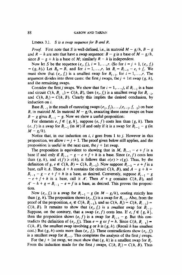
DEFINITION 3.3. Let B be a base and let R be a set of red elements such that R plus the red elements of B form an independent set. Order the elements of R as hi, i = 1,. . . , t, so that the cost is nondecreasing. Let H, = B. Supposegi and Hi, i = l,...,r, are such that Hi = Hi-, - gi + hi and ( gi, hi) is a smallest swap for hi and Hi-i. Then (g,, hi), i = 1,. . . ,r, is a restricted swap sequence (for B and R).
The term “restricted swap sequence” derives from the fact that we have restricted the order in which the red elements get swapped into the base. Also note that the initial condition given on R is for notational convenience only. One consequence is that 1 RI becomes the length of a swap sequence. Figure 3.1 shows a restricted sequence.
Note that a restricted swap sequence for B and R always exists, i.e., for each element hi, there is a swap (gi, hi): The circuit C(h,, Hi-i) contains a
HO HI = Ho-2+3 Ii2 = H,-9r4
H3:H2-I+5 H4= H+3+6
FIG. 3.1. Restricted swap sequence.

90 GABOWANDTARJAN
green element, since the red elements of B and R are independent. Now gj exists as a largest green element of C(h,, Hi-,).
In Figure 3.1, for i = 1,2,3, Hi is not a base in the optimum set j3,. However a restricted sequence does give the desired swaps:
COROLLARY 3.4. A restricted swap sequence for B and R can be re- arranged to form a swap sequence for B and R.
Proof. The proof is by induction on r. The base case r = 0 is vacuous. For r > 0, Lemma 3.1 shows (gi, hi) is in a swap sequence, where the remaining swaps form a swap sequence for B - g, and R - h, in matroid M - g,/h,. It is easy to check that (g,, h,), i = 2,. . . ,r is a restricted swap sequence for B - g, and R - h,. By induction these swaps rearrange to a swap sequence. The desired conclusion follows. 0
To actually form the swap sequence, order swaps (gi, hi) of a restricted sequence as follows: Sort (gi, hi), i = 1,. . . ,r so that their cost is nonde- creasing and for swaps (g,, hi) of equal cost, the index i is increasing.
COROLLARY 3.5. A restricted swap sequence, ordered as above, is a swap sequence.
Proof. Argue as in Corollary 3.4. 0
For some matroids Corollaries 3.4 and 3.5 give the best way to solve our problem. For other matroids a divide-and-conquer approach can be more efficient. We modify the results for this approach as follows: Choose B and R as in Definition 3.3. Let R, contain the [r/2] smallest elements of R, R, = {hi(i = l,..., 1 r/2] }. Let R, contain the remaining elements, R, = {hili = [r/21 + 1,. . . ,r }. Let G, be a set of 1 r/2] green elements such that B - G, + R, is a smallest base whose red elements are exactly the red elements of B U R,. Let G, be a subset of the remaining green elements of B such that B - (G, U G,) + R is a smallest base whose red elements are exactly the red elements of B U R.
Intuitively we expect that a restricted sequence swaps elements of G, with elements of R,, and similarly for G, and R,. This is correct except for slight complications due to equal-cost elements. So in the matroid M - R,/G,, let S, be a restricted swap sequence for base B - G, and red elements R,. Let G; = { gl (g, h) is in S, }. (As indicated above, it is not necessarily true that G, = G;.) In M - G;/R,, let S, be a restricted swap sequence for B - G; and R,. Let SiS, be the sequence formed by concatenating S, onto the end of S,.
COROLLARY 3.6. S,S, is a restricted swap sequence and thus can be ordered to form a swap sequence for B and R.
MATROID INTERSECTION PROBLEMS 91
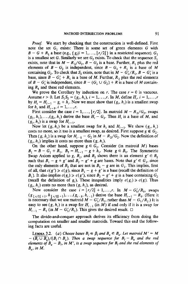
Proof. We start by checking that the construction is well-defined. First note the set G, exists: There is some set of green elements G with B - G + R, a base (e.g., { g,li = 1,. . . , [r/2] } in a restricted sequence). G, is a smallest set G. Similarly we see G, exists. To check that the sequence S, exists, note that in M - R,/G,, B - G, is a base. Further, R, plus the red elements of B - G, is independent, since B - G, + R, is a base of M containing G,. To check that S, exists, note that in M - G;/R,, B - G; is a base, since B - G; + R, is a base of M. Further, R, plus the red elements of B - G; is independent, since B - (G, U G2) + R is a base of M contain- ing R, and these red elements.
We prove the Corollary by induction on r. The case r = 0 is vacuous. Assume r > 0. Let S,S, = (g,, hi), i = 1,. . . , r. In 44, define Hi, i = 1,. . . , r by Hi = Hi-, - gi + hi. Now we must show that (gi, hi) is a smallest swap for hi and H,-i, i = l,..., r.
First consider the case i = 1,. . . , 1 r/2]. In matroid M - R,/G,, swaps (gp &I,. * -, (gi, hi) derive the base Hi - G,. Thus Hi is a base of M, and (gi, hi) is a swap for Hi-,.
Now let (g, hi) be a smallest swap for hi and Hi-,. We show (gi, hi) costs no more, so it too is a smallest swap, as desired. First suppose g e G,. Then (g, hi) is a swap for Hi-, - G, in M - R,/G,. Now the definition of (gi, hi) implies it costs no more than (g, hi).
On the other hand, suppose g E G,. Consider (in matroid M) bases B, = B - G, + R,, B2 = Hi-, - g + hi. Note g E B,. The Symmetric Swap Axiom applied to g, B,, and B, shows there is an element g’ E B, such that B, - g + g’ and B2 - g’ + g are bases. Note that g’ E G,, since the only elements of B2 that are not in B, - g are in G,. This implies, first of all, that c( g’) 2 c(g), since B, - g + g’ is a base (recall the definition of B,). It also implies c( gi) 2 c( g’), since B2 - g’ + g is a base containing G, (recall the definition of gi). These inequalities imply c( gi) > c(g). Thus ( gi, hi) costs no more than (g, hi), as desired.
Now consider the case i = [r/2] + 1,. . . ,r. In M - G;/R,, swaps
(qr,2] +19 hk,2’+1 ),. , . ,(gi_l, hipI) derive the base Hi-, - R,. (Here it is necessary t at we use matroid M - G;/R,, rather than M - G,/R,.) It is easy to see (g, hi) is a swap for HiPi (in 44) if and only if it is a swap for Hi _ I - R, (in M - G;/R,). This gives the desired result. 0
The divide-and-conquer approach derives its efficiency from doing the computation on smaller and smaller matroids. Toward this end the follow- ing facts are useful.
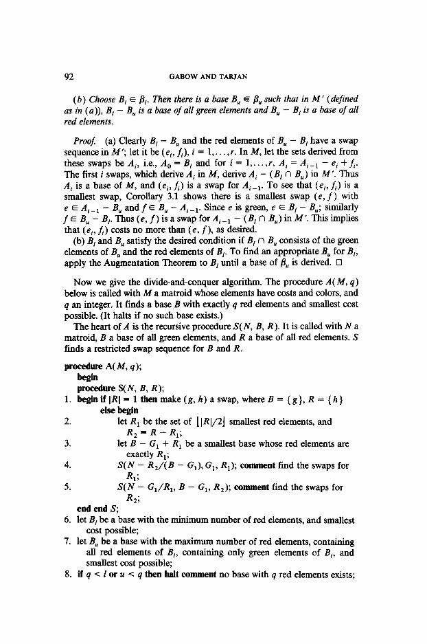
LEMMA 3.2. (a) Choose bases BI E /3[ and B, E B,. Let matroid M’ = M - (BI u B,)/(B, n B,,). Then a swap sequence for B, - B,, and the red elements of B, - B,, in M’, is a swap sequence for B, and the red elements of B,, in M.
92 GABOW AND TARJAN
(6) Choose B, E B,. Then there is a base B, E & such that in M’ (defined as in (a)), B, - B,, is a base of all green elements and B, - B, is a base of all red elements.
Proof: (a) Clearly B, - B,, and the red elements of B,, - B, have a swap sequence in M’; let it be ( ei, f,), i = 1,. . . ,r. In M, let the sets derived from these swaps be Ai, i.e., A, = B, and for i = 1,. . . ,r, Ai = Aiel - ei + fi. The first i swaps, which derive Ai in M, derive Ai - (B, n B,,) in M’. Thus Ai is a base of M, and (ei, fi) is a swap for Aiel. To see that (ei, h) is a smallest swap, Corollary 3.1 shows there is a smallest swap (e, f) with e E Ai- - B,, and f E B, - Ai _ i. Since e is green, e E B, - B,; similarly fEB,-B,.Thus(e,f)isaswapforA,_,-(B,nB,)inM’.Thisimplies that (ei, 6) costs no more than (e, f ), as desired.
(b) B, and B,, satisfy the desired condition if B, n B,, consists of the green elements of B, and the red elements of B,. To find an appropriate B, for B,, apply the Augmentation Theorem to B, until a base of Is, is derived. q
Now we give the divide-and-conquer algorithm. The procedure A(M, q) below is called with M a matroid whose elements have costs and colors, and q an integer. It finds a base B with exactly q red elements and smallest cost possible. (It halts if no such base exists.)
The heart of A is the recursive procedure S( N, B, R). It is called with N a matroid, B a base of all green elements, and R a base of all red elements. S finds a restricted swap sequence for B and R.
procedure A( M, q);
begin p=*e s(N, B, RI;
1. beginifIRI=lthe nmake(g,h)aswap,whereB={g},R={h} else begin
2. let RI be the set of [I RI/21 smallest red elements, and R, = R - R,;
3. let B - G, + RI be a smallest base whose red elements are exactly R,;
4. S( N - R2/( B - G,), G,, R,); comment find the swaps for R,;
5. S(N - G/R,, B - G,, R,); comment find the swaps for R,;
end end S; 6. let B, be a base with the minimum number of red elements, and smallest
cost possible; 7. let B,, be a base with the maximum number of red elements, containing
all red elements of B,, containing only green elements of B,, and smallest cost possible;
8. if q < I or u < q then halt comment no base with q red elements exists;

MATROID INTERSECTION PROBLEMS 93
9. S(M - (B, u B,J/(B, n 41, B, - B,,, B,, - 4); 10. let W contain the q - 1 smallest swaps found by S;
let G contain the green elements of swaps of W; let R contain the red elements of swaps of W,
11. B: = Bl - G + R comment B is the desired base end A;
Figure 3.2 illustrates the algorithm on Fig. 2.1. The initial call to S finds the base of Fig. 3.2a, resulting in recursive calls on the graphs of Figure 3.2b. The algorithm eventually finds the swaps of Fig. 2.2.
For the algorithm to work correctly we must break ties in cost con- sistently, as in Corollary 3.5. We shall see below (Lemmas 4.1, 6.1) that in most applications of the algorithm there is sufficient time to sort. Thus we use the simple rule of Corollary 3.5: Assume the red elements have been sorted and indexed in nondecreasing order. Then in line 2, choose the 1) RI/21 elements of R with smallest index. In line 10, if there is a tie for the q - Ith smallest swap, choose the one whose red element has smaller index for W. (An alternate approach to tie-breaking is given in Section 4.2.)
THEOREM 3.2. Procedure A finds a smallest base with exactly q red elements, if one exists.
Proof. We first check that procedure S is correct: when called with B a base of all green elements and R a base of all red elements, S finds a restricted swap sequence. We prove this by induction on 1 RI. The case 1 RI = 1 is handled correctly by line 1.
For ) RI > 1, lines 2-5 find the restricted swap sequence S,S, of Corollary 3.6: The entrance conditions on B and R imply that the set Gz of Corollary 3.6 is B - G, in the algorithm. By induction the recursive call of line 4 constructs S,. It is easy to see that the set G; of Corollary 3.6 is G, in the algorithm. By induction the recursive call of line 5 constructs S,. Thus S works correctly.
Now we show that A is correct. Lemma 3.2(b) shows bases B, and B, of lines 6-7 exist. In line 9, S finds a restricted swap sequence for B, and B,,,
(0) (b)
FIG. 3.2. Algorithm A. (a) B - G1 + R,, (b) The two recursive calls.

94 GABOW AND TARJAN
by Lemma 3.2(a). Line 11 finds the desired base B, by Corollary 3.5 and the Augmentation Theorem. 0
Now we examine the efficiency of algorithm A. We do not derive a general time bound, since more accurate bounds can be given for specific matroids. We start by discussing three properties of the matroid that are desirable for an efficient implementation.
First, the divide-and-conquer approach of A depends on the ability to contract and delete efficiently. Specifically, these operations are needed in lines 4, 5, and 9.
Second, A needs an efficient algorithm for finding a minimum-cost base. This algorithm can be used for lines 3,6, and 7. For instance line 6 is done as follows: Delete all red elements and find a smallest base B,. Then contract B, and find a smallest base B2. Finally set B, = B, U B,. Lines 3 and 7 are done in a similar way. (Another way to do lines 3, 6, 7, without contracting or deleting, is to modify the cost function so the desired base has minimum cost.)
The third desired property concerns the greedy algorithm. This algorithm, which finds a smallest base on any matroid, works as follows [Ll, pp. 275-2771: It is given a list of all elements, sorted so the cost is nonde- creasing. It prunes the list to the desired base, by scanning it from beginning to end, deleting any element that forms a circuit with previous (undeleted) elements of the list.
Specific matroids often have algorithms that are faster than the greedy one. These of course are the methods of choice for lines 6 and 7. However, the greedy algorithm is particularly suited for line 3. Even though line 3 is repeated many times in the recursion, the sort required by the greedy algorithm need only be done once. The details are as follows.
Procedure S is called with bases B and R given as sorted lists. Line 3 finds the desired base by running the greedy algorithm on the list of elements of R, followed by the list of elements of B. The sorted lists for the recursive calls of lines 4 and 5 are easily constructed. Thus in procedure S, no sorting is done for the greedy algorithm. Instead, linear-time list manipulation is done inside S, and one sort is done before the first call to S.
This brings us to the third desirable property of the matroid: The greedy algorithm runs faster than other minimum-cost base algorithms if the elements are given in sorted order.
We illustrate the efficiency of algorithm A by deriving a time bound for graphic matroids. Here the problem is to find a smallest spanning forest with q red edges.
Graphic matroids have the three properties that allow efficient implemen- tation of A. First, contraction and deletion are efficient, each requiring time O(m + n). Here we assume the graph is represented by adjacency lists. To
MATROIDINTERSECTIONPROBLEMS 95
contract a set of edges, form adjacency lists for the new graph, using a linear connectivity algorithm [AHU]. Further, for each edge in the contracted graph, record the edge in M (the original graph input to A) that it derives from. This is necessary so that when swaps are formed in line 1 of A, the swaps consist of edges of M.
Note that contractions may introduce parallel edges in the graph. How- ever, it is easy to see that in A, there are at most two parallel edges, one of each color, between two given vertices. Actually, we can allow the input graph M to contain such parallel pairs.
Concerning the second property needed to implement A, there are efficient algorithms for finding a minimum-cost spanning forest, in time owoglog(2+,,,, 1 n time [CT, T2, Y]. And for the third property, the greedy algorithm (i.e., Kruskal’s algorithm for minimum spanning trees) is even faster, O(ma(m, n)), if the edges are already sorted [AHU, pp. 172-1761.
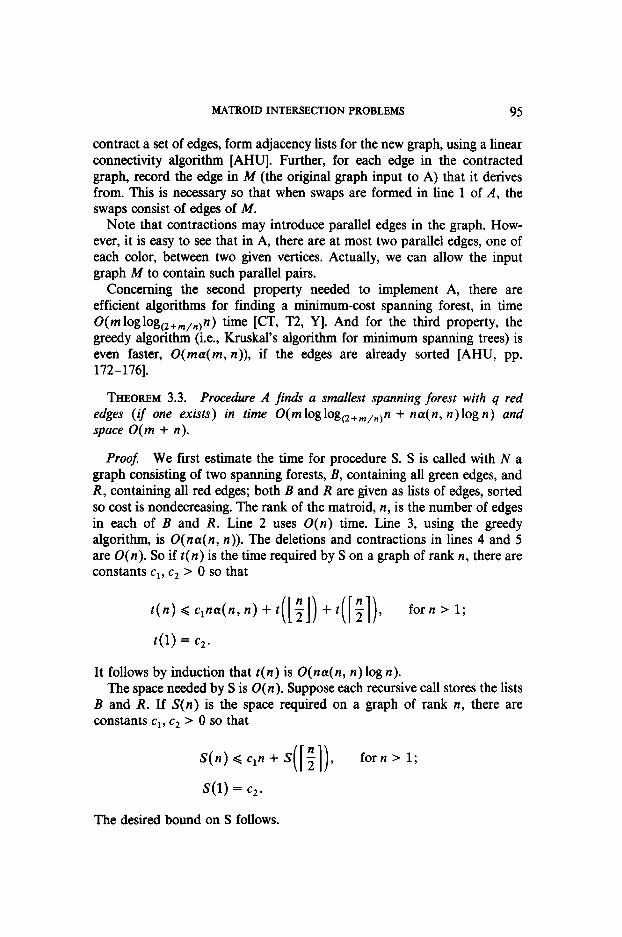
THEOREM 3.3. Procedure A fina!v a smallest spanning forest with q red edges (if one exists) in time O(mloglog~,+,,,,n + na(n, n)logn) and space O(m + n).
Proof We first estimate the time for procedure S. S is called with iV a graph consisting of two spanning forests, B, containing all green edges, and R, containing all red edges; both B and R are given as lists of edges, sorted so cost is nondecreasing. The rank of the matroid, n, is the number of edges in each of B and R. Line 2 uses O(n) time. Line 3, using the greedy algorithm, is O(na(n, n)). The deletions and contractions in lines 4 and 5 are O(n). So if t(n) is the time required by S on a graph of rank n, there are constants ci, c2 > 0 so that
t(n) d qna(n, n) + t (13) + tM)~
for n > 1;
t(1) = c*.
It follows by induction that r(n) is O(na(n, n) log n). The space needed by S is O(n). Suppose each recursive call stores the lists
B and R. If S(n) is the space required on a graph of rank n, there are constants ci, c2 > 0 so that
S(n) < cln + S (I 1)
; , forn > 1;
s(1) = cq.
The desired bound on S follows.

96 GABOW AND TARJAN
Now suppose A is called on a graph of rank n, with m edges. Lines 6-7, using an efficient minimum spanning tree algorithm, are O(m log logC,+,,,,n). Line 9 is O(na(n, n)log n). (This includes the time to sort the edges in the spanning forests B, - B,, and B, - B,.) Line 10 is O(n), using a linear selection algorithm [BFPRT, SPP]. The desired time bound for A follows. The space is obvious. 0
The next section improves this time bound by eliminating the factor a( n, n) in the second term. Subsequent sections apply A to other matroids. The efficiency can be estimated by computations similar to Theorem 3.3.
Sections 4-6 all use algorithms that are variants of A. One simple variant is to replace procedure S by a procedure that computes a restricted swap sequence directly from Definition 3.3. This approach, coupled with data structures and algorithms that capitalize on special features of the matroid, often gives our best algorithms.
4. GRAPHIC MATROIDS
This section discusses our problem on graphic matroids. As mentioned before, the problem here is to find a smallest spanning forest with q red edges. First we use the “dynamic tree” data structure of Sleator and Tarjan [ST] to solve the problem in O(m loglog,,+,,,,n + n log n) time. Then we discuss a special case of the problem-finding a smallest spanning tree with a degree constraint. We show this case is linear-time equivalent to finding an (unconstrained) minimum spanning tree.
4.1. Spanning Forests
This section shows that for graphic matroids a restricted swap sequence can be rapidly computed from the definition. It also gives a lower bound to show that no implementation of the swap sequence approach can be faster.
The dynamic tree data structure allows a number of operations, including the following:
find max (u) return an edge of maximum cost on the tree path from u to the root;
euert (0) modify the tree so that u is the root; cut (u, w) delete the tree edge (u, w); fink (u, w, x) link the trees containing u and w by adding edge
(u, w), setting the cost of (u, w) to x.
The time for a series of m such operations is O(n + m log n) [ST]. It is easy to see how to use these operations to compute a restricted swap
sequence. We maintain the tree T so that any red edge in T has a modified
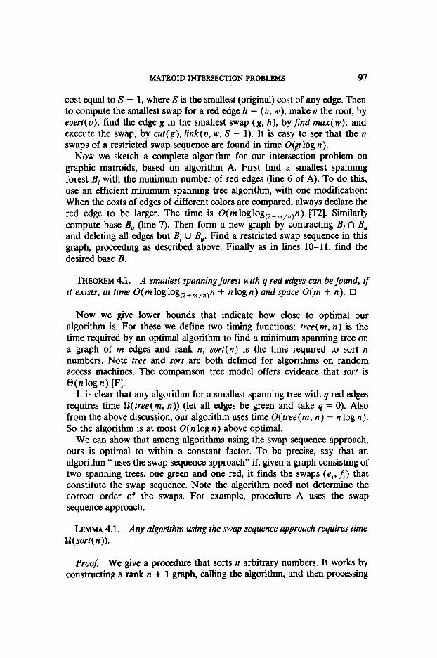
MATROID INTERSECTION PROBLEMS 97
cost equal to S - 1, where S is the smallest (original) cost of any edge. Then to compute the smallest swap for a red edge h = (u, w), make u the root, by euert( u); find the edge g in the smallest swap (g, h), by find max( w); and execute the swap, by cut(g), link(u, w, S - 1). It is easy to seHhat the n swaps of a restricted swap sequence are found in time O&l& n).
Now we sketch a complete algorithm for our intersection problem on graphic matroids, based on algorithm A. First find a smallest spanning forest B, with the minimum number of red edges (line 6 of A). To do this, use an efficient minimum spanning tree algorithm, with one modification: When the costs of edges of different colors are compared, always declare the red edge to be larger. The time is O(mloglogo+,,,,n) [T2]. Similarly compute base B,, (line 7). Then form a new graph by contracting B, fl B, and deleting all edges but B, U B,,. Find a restricted swap sequence in this graph, proceeding as described above. Finally as in lines 10-11, find the desired base B.
THEOREM 4.1. A smallest spanning forest with q red edges can be found, if it exists, in time O(m log log,,+,,,, n + nlogn) andspace O(m + n). 0
Now we give lower bounds that indicate how close to optimal our algorithm is. For these we define two timing functions: tree(m, n) is the time required by an optimal algorithm to find a minimum spanning tree on a graph of m edges and rank n; sort(n) is the time required to sort n numbers. Note tree and sort are both defined for algorithms on random access machines. The comparison tree model offers evidence that sort is @(n log n) [F].
It is clear that any algorithm for a smallest spanning tree with q red edges requires time Q( tree( m, n)) (let all edges be green and take q = 0). Also from the above discussion, our algorithm uses time 0( tree(m, n) + n log n). So the algorithm is at most 0( n log n) above optimal.
We can show that among algorithms using the swap sequence approach, ours is optimal to within a constant factor. To be precise, say that an algorithm “ uses the swap sequence approach” if, given a graph consisting of two spanning trees, one green and one red, it finds the swaps (ei, A) that constitute the swap sequence. Note the algorithm need not determine the correct order of the swaps. For example, procedure A uses the swap sequence approach.
LEMMA 4.1. Any algorithm using the swap sequence approach requires time Sl(sort(n)).
Proof. We give a procedure that sorts n arbitrary numbers. It works by constructing a rank n + 1 graph, calling the algorithm, and then processing

98 GABOWANDTARJAN
the swaps given by the algorithm to find the sorted order. Excluding the time for the algorithm, the procedure uses O(n) time. Since tin < sort(n) =G sort(n - 1) + czn this suffices to prove the Lemma.
Consider n numbers xi,. . . ,x,. Without loss of generality assume all numbers are positive (otherwise increase the numbers by a constant). Let it4 be the largest of these numbers plus one. The graph for xi,. . . ,x, is shown in Fig. 4.1. Formally, the graph has vertices U, w, and ui, i = 1,. . . , n; green edges (u, ui) costing -x, and red edges (w, ui) costing x,, i = 1,. . . ,n; green edge (u, w) costing 0 and red edge (u, w) costing M.
To specify the swap sequence of this graph, let the given numbers in nondecreasing order be y,, . . . , y,,. Then identifying each edge by its cost, the swapsequenceis(O,yI),(-yI,y2),...,(-y,-,,y,),(-y,,M).
The procedure constructs the graph and calls the algorithm to find the swaps of the swap sequence. Then it encodes the swaps into an array S, by setting S(i) = j if ((u, ui), (w, uj)) is a swap, and S(0) = j if ((u, w), (w, uj)) is a swap. Finally it outputs the sequence S(O), S2(0), . . . , S”(0). It is easy to see this gives the indices of the numbers in sorted order. Furthermore, the time spent before and after the algorithm is O(n), as desired. 0
COROLLARY 4.1. Any algorithm that fin& a smallest spanning tree with q red edges using the swap sequence approach requires time Q( tree( m, n) + sort(n)). 0
FIG. 4.1. Lower bound graph.
MATROID INTERSECTION PROBLEMS 99
4.2. Spanning Trees with a Degree Constraint
Now we turn to a special case of our problem on graphic matroids that has some practical significance. An important question in network design is how to link a central computer, having a limited number of communication channels, to a collection of peripheral computing sites. Some versions of this problem, such as the Capacitated Tree Problem, are NP-complete [PI. Closely related but tractable is the problem of finding a smallest spanning tree such that a given vertex u has a specified degree. Polynomial algorithms have been presented for this problem [GK]; the most efficient uses time wm w%(,+m,n, n + n log n) [Gal]. We show here that the problem is equivalent to finding a minimum spanning tree. More precisely, we give an algorithm for the problem that finds one minimum spanning tree and then does O(n) postprocessing.
An exact statement of the degree-constrained spanning tree problem is as follows: Given a connected graph with real-valued edge costs, find a spanning tree with smallest possible cost such that the degree of a given vertex u is exactly p. We solve the following problem: Given a connected graph with edge costs and colors, such that all green edges are incident to u, find a smallest spanning tree with q red edges. This problem includes the degree-constrained spanning tree problem if we take q = n - p, but it allows red edges incident to u. (Note that in both problems the restriction to connected graphs is for convenience only.)
The problem is simplified by making the desired tree unique. This can be done in a variety of ways. Here we take the desired tree to be lexicographi- tally minimum. That is, assume the edges of the graph are indexed from 1 to m. For any set of edges, form a vector by arranging its edge indices in increasing order, i.e., for { e,,, ei2,. . . , ei, } where i, < i, < . . . < i,, form (il, i,,. . . , ik). Now among all smallest spanning trees with q red edges, our algorithm finds the one whose vector is lexicographically minimum.
Note that this tree is the unique smallest spanning tree with q red edges with respect to a certain cost function c’. To define c’, set E = (1/(2m))(min{ ]c(S) - c(T)I: S, T are sets of edges, IS] = (TI, c(S) Z c(T)} u {l}), and c’(ei) = c(ei) - 8. Then for any two sets S, T with ISI = ITI, c’(S) < c’(T) if and only if c(S) < c(T) or c(S) = c(T) and S is lexicographically smaller than T. This implies the desired property of c’.
Note also that no two swaps have the same cost c’: It is easy to check that c’(ei, ei) < c’(ek, e,) if either c(ei, ei) < c(ek, e,) or c( ei, ej) = c(ek, e,) and the vector for { ej, ek } is smaller than the vector for { ei, ep }.
In the lemmas that follow, we assume the cost function c has been changed to c’. Hence no two edges or swaps have the same cost. In the algorithm, we can use c’ without explicitly calculating it, by using the characterization of c’ in terms of c specified above.
We make two more assumptions. First, the green edges form a spanning tree. Second, some of the red edges form a spanning tree, and the red edges
100 GABOW AND TARJAN
not in the tree are incident to u. (Note that by preprocessing as in procedure A, the general case reduces to the case where the green and red edges are spanning trees. We shall see that our algorithm may introduce extra red edges incident to u.)
Now let q;, i = 0,. . . , n be the smallest sparming tree with exactly i red edges. Let q = T-i - e, + fi, i = 1,. . . ,n, so that (ei, f,), i = 1,. . . ,n, is the swap sequence. As noted above, I;:, ei, and f. are unique.
Our approach is to start with T, and repeatedly find sets of edges that are in the first q swaps. We do not find the swaps themselves. The following simple concept is central in deducing the edges in swaps.
DEFINITION 4.1. For a green edge e = (u, w), let r(e) be the smallest red edge incident to w. Equivalently, (e, p(e)) is the smallest swap for e and T,.
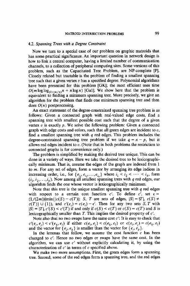
Note p(e) always exists, since the red edges span. Let M = {(e, p(e)) le is green}. The M-swaps for a graph are shown in Fig. 4.2. The next four lemmas show how the M-swaps allow us to deduce edges in T4.
LEMMA 4.2. Suppose (e, p(e)) is not a valid swap for some optimal tree !& 0 < i d n. Then p(e) E T.
Proof Choose i as small as possible such that (e, p(e)) is not valid. Clearly i > 0. It suffices to prove the lemma for q, since this implies p(e) E q forj > i.
First note that either e e q or p(e) E T. For otherwise e E q and p(e) 4 I;:. Since (e, p(e)) is not valid, the cycle C@(e), ‘I;) does not contain e. This implies C(r(e), q) does not pass through U. But then C( p( e), q) consists entirely of red edges, contradicting the fact that the red edges not incident to v are acyclic.
Thus without loss generality e 4 T. Hence q derives from T-i by doing the smallest swap for e. (e, p(e)) is valid for q-i, by definition. Thus Corollary 3.2 implies it is the smallest swap for e, and p(e) E 1;:. 0
LEMMA 4.3. If (e, p(e)) is among the q smallest swaps of M, then
de> E Tq.
6
FIG. 4.2. A graph with M = {(5,6), (4,6),(3,8), (1,7), (9,15), (2, lo)} and F = (6,8,2}.

MATROID INTERSECTION PROBLEMS 101
FIG. 4.3. T3 for Fig. 4.2.
Proof Among the first 4 swaps (ei, A), i = 1,. . . ,q of the swap se- quence, there is one with c(ei, p( ei)) 2 c(e, r(e)). Corollary 3.2 implies c(q, fi) 2 de, de)).
Now if (e, p(e)) is a valid swap for q-i, it is the smallest swap, and thus (e, p(e)) = (ei, fi). (Recall no two swaps have the same cost.) Hence p(e) E Tq. Otherwise, if (e, p(e)) is not valid, Lemma 4.2 implies p(e) E T,. cl
In Fig. 4.2, the. lemma implies edges 6 and 8 are in T,, as shown in Fig. 4.3. Notice the lemma does not give q = 3 distinct red edges in T4. In general, the lemma need only give [q/2] red edges, since a red edge can be the p-value of two green edges.
LEMMA 4.4. Zf (e, p(e)) is not among the 2q - 1 smallest swaps of M, then e E T4.
Proof: We argue by contradiction. Suppose e $5 T4. Then some swap (ei, fi), i = l,..., q, in the swap sequence has ei = e. From Corollary 3.2, c(e, p(e)) < c(e,, fi). Clearly none of the 2q - 1 swaps of A4 that are strictly smaller than (e, p(e)) is valid for T _ i. These swaps contain at least q distinct red edges, and Lemma 4.2 shows they are all in q-i. Since i - 1 < q, this is the desired contradiction. 0
This Lemma is illustrated by edge 2 in Figs. 4.2 and 4.3. Lemmas 4.3 and 4.4 allow us to deduce edges in T4. Now we show how
these lemmas can be iterated. Let F be any set of edges in T4. Form a multigraph H as follows. First form G/F. In a slight abuse of notation, let u denote the vertex of G/F that contains the original vertex u of G. If G/F contains parallel edges, they are incident to u (since two parallel edges not incident to u give a cycle of red edges in G - u, a contradiction). Now for every set of parallel edges (all incident to u) of the same color, delete all but the edge of smallest cost. The resulting multigraph is H. (This is illustrated in Fig. 4.4a.) We show that T4 corresponds to an optimal tree in H. Let p be the number of red edges in F.

102 GABOW AND TARJAN
IO I’ I’\
cl
a 18 \’
3” \I ’ ,9 \‘\
/’ ’ ‘1 ‘\I ‘,9
’ ‘\
7 + b
15
(a)H (b) T3-F
FIG. 4.4. Derived graph for Fig. 4.2.
LEMMA 4.5. In the multigraph H, the edges T4 - F form the smallest spanning tree with q - p red edges.
Prooj: First note that all edges of T4 - Fare in H; i.e., none are deleted. For if an edge e E T4 is parallel to an edge f, clearly f 4 T4, since Tq is acyclic. If f has the same color as e but smaller cost, then the spanning tree T4 - e + f contradicts the definition of Tq. So e is not deleted.
Now it is clear that T4 - F is a sparmmg tree of H containing q - p red edges. Further, it is the smallest such tree. For if S is a smaller tree, then S + F is a spanning tree of G that contradicts the definition of T4. 0
Figure 4.4 shows H and T3 - F, the smallest spanning tree with one red edge. Note that in H, the smallest spanning tree with no red edges is {1,3,9}. This tree corresponds to a spanning tree of G with two red edges, { 1,2,3,6,8,9}, but this is not T2 = {1,2,3,6,7,9}.
The last result allows us to iterate Lemmas 4.3 and 4.4 until all edges of T4 are deduced. This is the method followed by procedure B given below.
On entry to B, the graph (a multigraph) consists of two spanning trees, one green and the other red. All green edges are incident to u; red edges may or may not be incident to u. A spanning tree containing q red edges is to be found. (By assumption, such a tree exists.)
B adds edges to a list F until it is the desired tree. q is maintained as the number of red edges to be added.
procedure B; begin
1. while the graph has more than one vertex do begin
2. for each green edge e = (u, w) do p(e): = the smallest red edge incident to w;
3. let M = {(e, p(e))le is a green edge}; let Mi contain the q smallest swaps of M; let M2 contain all but the 2q - 1 smallest swaps of M;

MATROID INTERSECTION PROBLEMS 103
4. add the red edges of swaps of MI to F, decrease q by the number of edges added;
5. add the green edges of swaps of M2 to F; 6. contract the edges of F; 7. for each vertex of the graph w # u do
delete all edges from w to u except the smallest green and smallest red edge (if it exists);
end end B;
When B is called with q = 3 in Fig. 4.2, the first iteration forms the graph of Fig. 4.4a; the second iteration adds the edges of Fig. 4.4b to F, completing the tree T3.
Note that in lines 2, 3, and 7, ties in cost c are broken lexicographically, consistent with the cost function c’ described at the start of this section.
Also in line 6, it is only necessary to contract the edges added to F in the current iteration. As usual, we do the contraction by forming adjacency lists for the new multigraph. Further, for each edge in the current graph we record the edge in the original graph from which it derives. This way we can maintain F as a list of edges in the original graph.
LEMMA 4.6. Suppose B is called with the entry conditions (given above B) satisfied. Then B adds edges to F that form the smallest spanning tree with q red edges. B runs in O(n) time and space.
Proof: We first prove correctness. We show that every time line 1 is reached, the following conditions hold:
(i) The desired tree consists of F plus the smallest spanning tree with q red edges in the current graph.
(ii) The green edges form a spanning tree, with each green edge incident to u.
(iii) The red edges consist of a spanning tree and zero or more edges incident to u.
The entry conditions show (i)-(m) hold initially. So suppose lines 2-7 are executed. The edges added to F in lines 4-5 are in the desired tree, by Lemmas 4.3 and 4.4. (Note if q = 0, line 5 adds all green edges to F, as desired.) Lines 6-7 form the graph H of Lemma 4.5. Hence after line 7, (i) holds. Condition (ii) is obvious. To see (iii), first note that the red edges not incident to D in the new graph are acyclic (otherwise the original graph has a red cycle missing u). Further, the red edges span the new graph. Condition (in) follows. This completes the induction.
Finally note that every time through the loop, if q > 0 the iteration decreases q, if q = 0, the loop halts. Thus B eventually halts. Now (i) shows F is as desired.
104 GABOW AND TARJAN
Now we estimate the efficiency of B. First observe that one iteration of lines 2-7 takes time linear in the number of edges (in the current graph). Line 3 uses a linear-time selection algorithm [BFPRT, SPP].
Define the following quantities, for i 2 1: qi is the value of q immediately before the ith iteration of the while loop; gi (ri) is the number of green (red) edges in the graph immediately before the i th iteration. The following relations hold, for i >/ 1:
(l) 4i+l d 4d29
C2) gi+l d 2qi - ‘3
(3) ri 6 2g, - 1.
Relation (1) holds because the i th iteration adds the red edges of Mi to F. Relation (2) holds because the ith iteration adds the green edges of M2. Relation (3) follows from inductive assertions (ii) and (iii).
Now the i th iteration uses time 0( gi + I;). For i = 1 this is O(n), by (ii) and (iii). Otherwise (2) and (3) show that for i 2 1, ri+i and gi+i are both 0( qi). Condition (i) shows qi G qJ2’ -’ d n/2’ -i. Hence all iterations after the first take time at most a constant times CT=in/2’-’ = O(n). This gives the desired time bound.
The space bound is obvious. (Note that we only maintain adjacency lists for the current graph.) 0
The main routine for finding a degree-constrained sparming tree is similar to procedure A: First find trees Tl and T, (lines 6-7 of A). Then check q for feasibility (line 8). If q is feasible, decrease its value by 1, and place the I red edges of T, in F. Then delete ail edges besides q U T,, and contract q n T,. After this step the green edges and the red edges both are spanning trees. Finally call B.
THEOREM 4.2. The above algorithm firA a smallest spanning tree with a degree constraint, in time 0( m log log(,+ m,njn) and space O(m).
Proof; T/ and T, are found by using a minimum spanning tree algorithm on the graph with edge costs appropriately modified. The time for this is OWWog~2+,~,~ n > t CT, Y, T2]. The new graph can be constructed from the O(n) edges in T, U T, in time O(n). B is O(n). The time bound follows. q
Actually the algorithm can be implemented with only one call to a general minimum spanning tree algorithm. First find T,, the spanning tree with the greatest number of red edges and smallest cost possible. Use the general algorithm for this. Then find T,, the spanning tree with the fewest number of red edges, containing all green edges of T,, only red edges of T,, and smallest cost possible. Note that after the cost function has been ap-
MATROIDINTERSECTIONPROBLEMS 105
propriately modified, this can be done by finding a minimum spanning tree on a graph consisting of a spanning tree T, and edges incident to one vertex u. This requires time O(n), by an algorithm originaIIy due to Spira and Pan: Use procedure B, with lines 2-5 replaced by one step that adds the smallest edge incident to each vertex in the graph to F. (Also, ignore colors in line 7). Details are in [SP, p. 3771. This gives the following result:
COROLLARY 4.2. A smallest spanning tree with a degree constraint can be constructed by modifying costs (in time O(m)), finding one minimum spanning tree, and doing O(n) postprocessing. 0
Note that finding a smallest spanning tree with a degree constraint requires at least the time to find a minimum spanning tree. (We can find a minimum spanning tree for a graph by adding a vertex u with one edge, and finding a smallest spanning tree with one edge incident to u.) Hence the two problems are linear-time equivalent.
5. MATCHING MATROIDS
This section discusses our intersection problem on several types of matching matroids. First the matroids are defined. Then an 0( m + n log n) algorithm is given for simple scheduling matroids. An O(m log n + n2) algorithm is given for general scheduling matroids. Finally, the time for general transversal and matching matroids is shown to be 0( m log m + ne).
We begin with the definitions. A matching matroid is derived from a graph G and a subset of the vertices J. The elements of the matroid are the vertices of J. The independent sets are subsets of J that can be covered by a matching of G. A transversal matroid is a matching matroid where G is bipartite and J is one of the two vertex sets of G (i.e., each edge goes from J to 7).
Two special types of transversal matroids are of particular interest. A (general) scheduling matroid derives from a convex bipartite graph. More precisely, the vertices of J can be indexed from 1 to ]j] so that each vertex of J is adjacent to consecutive vertices a, a + 1,. . . , b of .? (and no others). We think of the vertices of J as jobs and the ith vertex of 7 as the time period from i - 1 to i. Thus a scheduling matroid corresponds to the following situation: A processor runs for ]J] units of time. There are m = ] JI jobs, each requiring one unit of processing time. Each job j has a release time 5 and a deadline dj, both integers, 0 d 5 -C dj < I.?I. If jobj is chosen for execution, it must be started no earlier than time 5 and finished no later than dj. In this matroid a base is a set of jobs of maximum cardinality that can be executed on the processor so that each job meets its constraints. A

106 GABOW AND TARJAN
schedule is a base, together with a specification of when each job gets executed.
A simple scheduling matroid [Ll pp. 265-266, 2781 corresponds to a convex bipartite graph where each vertex of J is adjacent to vertices 172 , . . . , b, for some b. In the scheduling interpretation, each release time is 0, so release times can be ignored.
In the following discussion we use interval notation in two ways. The first is for intervals of time. Suppose a processor executes n unit-length jobs, one after another. We say that the ith job is executed in the time interval [i - 1, i). (Thus the ith job is no longer executing at time instant i.) The second use employs interval notation for sets of integers. Thus if r and d are integers, [r, d) denotes the integers in the set of real numbers usually denoted [r, d), i.e., [r, d) = {r,. . , , d - l}. The context will always make our use of interval notation unambiguous.
5.1. Simple Scheduling Matroids
This section discusses the following scheduling problem. Given is a set of m unit-length jobs. Each job has an integer deadline, a real-valued profit, and a job class G or R. The profit for a job is earned if and only if it is completely executed by its deadline. Find a maximum profit schedule containing exactly q jobs in class R.
This problem is essentially equivalent to our intersection problem on simple scheduling matroids. Note that we will give an algorithm that finds a schedule, not just an (unordered) base. Also, as usual, without loss of generality we find a minimum (not maximum) cost base (schedule). An example problem is shown in Fig. 5.1. Jobs are identified by their cost and listed underneath their deadline.
We represent the matroid by the following data structure. For each integer time t between 1 and the largest deadline, there is a list D, = { juobj has dj = t }. The list heads are in an array so that given t, the first job in Dt can be found in O(1) time. It is easy to construct this data structure in linear time from any reasonable specification of the matroid.
We start with a simple normalization: We can always assume that the processor runs from time 0 to n, and exactly n jobs are executed.
0 I 2 3 4
GREEN JOBS 2 5 3 7
RED JOBS I 6 6 4
FIG. 5.1. Simple job scheduling matroid, with swap sequence (7.1). (5,6), (2,4), (3,~.

MATROID INTERSECTION PROBLEMS 107
LEMMA 5.1. Let M be a simple scheduling matroid. Then there is a simple scheduling matroid M’, where M’ has rank n’ = max{ djl j is a job of M ‘}, m’ < (n’)‘, and for some set of jobs I of M, I plus a base of M’ gives a base of M (i.e., M’ = M/I). Further if the jobs have costs, then I plus a minimum cost base of M’ gives a minimum cost base of M. M’ can be found in time
O(m).
Proof. First we prune M to a matroid M’ with all the desired properties except the upper bound on m. To do this, initialize M’ to M and I to 0. Then set n’ = max{ djl j is a job of M’}. Now let J1 = { j] j is a job of M’ and dj > t }. Suppose there is a time t such that ]J,] = n’ - t. Then choose t as large as possible; remove the jobs of J, from M’ and add them to I; then repeat the process (start by redefining n’). Otherwise if there is no time t, halt.
The correctness of this procedure follows from the observation that the deleted sets J, are included in any base of M; also, the final matroid M’ has rank n’. It is easy to implement this procedure in linear time. (Note that without loss of generality the largest deadline in M is at most m. Also if we seek a schedule rather than just a base, the assignment of I to time periods can also be recorded in linear time.)
In the second modification to M’, for each d, 1 < d < n’, remove all but d smallest jobs that have deadline d. (If fewer than d jobs have deadline d, do not remove any. If jobs do not have costs, the choice of jobs to remove is arbitrary.) It is easy to see that this does not change the minimum cost of a base, and achieves the bound m’ 6 n’(n’ + 1)/2. Further this can be done in the required time by using a linear-time selection algorithm [BFPRT, SPP]. 0
For the rest of the discussion we assume the matroid has been pre- processed so M has the properties given above for M’.
Now we discuss finding a minimum-cost schedule. The greedy algorithm can be implemented in time O(m log m + n), or if the jobs are already sorted, O(m + n). This is a simple exercise using the UNION-FIND data structure [HS, pp. X1-168, GT2].
The time bound for unsorted jobs is improved to 0( m + n log n) by the following algorithm. Recall 0, = { jldj = t }. The algorithm also uses A, a priority queue of jobs.
procedure C; begin
1. A:= 0; 2. fort:= n to1 by -1 do
begin 3. A:= A U 0,;

108 GABOW AND TARJAN
4. remove the smallest job from A (if one exists), and schedule it in time interval [t - 1, t);
end end C;
LEMMA 5.2. Procedure C finds a minimum-cost schedule for a simple scheduling matroid in time O(m + n log n) and space O(m).
Proof: We start by showing that if j is a smallest job with deadline n, there is a minimum schedule with j executed in [n - 1, n). Suppose a minimum-cost schedule executes jobs k,, . . . ,k,, in that order. If j e
{k i,. . . , k,}, then the schedule k,, , . . , knel, j has the desired property (since c(j) G c(k,)). Otherwise if j = ki, the schedule k,, . . . ,ki -1, k. I+ i, . . . , k, _ i, j has the desired property.
Now it is easy to prove by induction on n that C finds a minimum-cost schedule. To verify the time bound for C, implement A and D,, t = 1,. . . , n, as mergeable heaps, e.g., 2-3 trees [AHU, pp. 152-1551. Then the opera- tions of union and removing the smallest are O(log m). The time bound follows. 0
It now follows that procedure A runs in time O(m + na(n, n)log n) on simple scheduling matroids3. The analysis is similar to that for spanning trees. Note that contraction is easy to do on a simple scheduling matroid: Suppose a set containing k, jobs of deadline i, i = 1,. . . ,n, is to be contracted. Then a job whose original deadline is d gets a new &a&e d - C;xlki.
Now we give an algorithm for the intersection problem on simple scheduling matroids that runs in 0( m + n log n) time. It works by comput- ing a restricted swap sequence from the definition. We start by characteriz- ing the valid swaps for a base B. For time t = 1,. . . , n, let b, be the number of jobs in B with deadline at most t. The slack in B at time t is t - 6,; B is tight at time t if t = b,. (Thus B is a base if and only if it has nonnegative slack at times 1 , . . . , n - 1 and is tight at n.)
LEMMA 5.3. Let B be a base, with jobs g E B, h G B. Choose t as small as possible so that t > d, and B is tight at t. Then B - g + h is a base if and only if d, Q t.
Proof. LetB’=B-g+h.B’isabaseifandonlyiffors=l,...,n, b,’ < s. We consider three cases.
If d, > t, then b,! = b, + 1 = t + 1, so B’ is not a base. If d, G d,, then for any s, s = 1 , . . . ,n, b,’ G b,, so B is a base. Finally suppose d, < d, G t. If s < d, or s >, d,, then b,’ = 6,. If d, G s < d,, then b,’ = b, + 1; the choice of t shows b; Q s. Hence B’ is a base. q
The Lemma implies that the following procedure can be used to find the best swap (g, h) for a base B and red job h.
‘See note added in proof.

MATROID INTERSECTION PROBLEMS 109
procedure D; begin
1. find the smallest time t > d,, where B is tight; 2. find the largest green job g E B with d, G t; 3. make(g,h)aswap;B:=B-g+h;
end D;
Note that time t exists, since B is a base. The green job g exists if there is any swap for h, and (g, h) is a largest swap, by the Lemma.
We will find a restricted swap sequence by iterating D. We use the following data structure for the base B: Take any balanced tree with n leaves, e.g., a complete binary tree. Number the leaves from left to right as 1 , . . . ,n. The leaves descending from a node s form an interval of integers 11, r]. Node s represents the corresponding time interval, [I - 1, r). Node s has three data fields: G(s) is the largest green job in B with a deadline in [I, r]. S(S) is an integer used to compute slacks; more precisely for any integer time t, if P is the path from leaf t to the root, then the slack of B at t is C uEPS(u). M(s) is the smallest sum CuepS(u), where P is a path from s to a leaf in [/, r]. (Thus for instance the root has M-value 0.)
Figure 5.2 illustrates this data structure for Fig. 5.1. Each node s is labeled with the values G(s), S(S), M(s). Figure 5.2a shows the data structure for the initial base of all green jobs; Figure 5.2b shows it after the first swap (7,1) has been made.
Besides the balanced tree, the green jobs of B are organized in lists: For each integer time t, 1 Q t d n, there is a list L(t) of all the green jobs in B with deadline t; L(t) is sorted so that cost is nonincreasing.
Using this data structure, it is easy to implement D in time O(log n) [AHU, pp. 145-1521. For example, the update to B in line 3 is done as
2.1.1 5,1.1 7.0.0-c0.I.I 2.0.0 5.1.1 3.1.1
(a) (b)
FIG. 5.2. Balanced tre-e for (a) B,, (b) B, - 7 + 1.
110 GABOW AND TARJAN
follows:
comment set B to B - g + h; 3.1. remove g from L(d,);
if L(d,) # IZI then G(d,):= the first job in L(d,) else G(d,): = 0 comment 0 is a dummy job with cost - cc;
3.2. increase S( dg) and M(d,) by 1; for each node s on the path from leaf d, to the root do
begin if s has a right brother r then increase S(r) and M(r) by 1; if s # d, then begin
let G(s) be the job with the largest cost in { G(s’)ls’ is a son of s}; M(s): = S(s) + min{ M(s’)ls’ is a son of s};
end end; 3.3. decrease S(d,) and M(d,) by 1;
for each node s on the path from leaf d, to the root do begin if s has a right brother r then decrease S(r) and M(r) by 1; M(s):= S(s) + min{ M(s’)ls’ is a son of s}; end;
The remaining details of procedure D are left to the reader. Now suppose we are given bases B and R of all green and all red jobs respectively. A restricted swap sequence for B and R can be found by sorting the jobs in B and in R, constructing the data structure for B, and iterating procedure D n times. This gives the following result.
LEMMA 5.4. A restricted swap sequence for two bases can be found in time 0( n log n) and space O(n). q
The complete algorithm for our intersection problem follows procedure A: First find bases B, and B, (lines 6-7). Then check q for feasibility (line 8). Find a restricted swap sequence as in line 9, only using the procedure given above. As in lines 10-11, form the desired base B by making the q smallest swaps. Finally construct a schedule for B in line@ time, as follows: Schedule jobs of B from the first time slot to the last, always choosing the job with smallest deadline to be executed next.
THEOREM 5.1. For simple scheduling matroidv, a smallest schedule with q red jobs can be found in time 0( m + n log n) and space O(m). 0
Note that our time bound is the same as the best known method for finding a minimum-cost base. (The time needed to do the latter is clearly a lower bound on the time for our intersection problem.) We can also show

MATROID INTERSECTION PROBLEMS 111
that our algorithm is the best possible implementation of the swap sequence approach. This is done below in Corollary 6.1.
5.2. General Scheduling Matroids
Now we treat the general scheduling problem, where each job j has a release time 5 and a deadline dj, Again we seek a smallest schedule with q red jobs.
We start by normalizing the matroid.
LEMMA 5.5. Let M be a general scheduling matroid. Then there is a general scheduling matroid M’, where M’ has rank n’ = max{ djl j is a job of M’}, m’ < (n’)3, and a base of M’ is a base of M. If the jobs have costs, a minimum-cost base of M’ is minimum for M. M’ can be found in time O(m log m) and space O(m).
The time bound of the Lemma is acceptable as a preprocessing cost, since the other algorithms of this section sort the jobs by cost and actually use more than 0( m log m) time. Nonetheless note that a more precise statement of the resource bounds for Lemma 5.5 is O(m) time and space, plus the time and space needed to sort the release times and deadlines. These are 2m integers between 0 and d, where d is the maximum deadline of a job in M. Thus using a bucket sort the time and space bounds are 0( m + d ); using a radix sort the time is 0( m log m d) and space is O(m).
Proof: First we find M’ satisfying all conditions except the upper bound on m’. In M, find a schedule with as many jobs as possible. M’ consists of the jobs of M with every release time and deadline t changed to the number of jobs scheduled in [0, t).
The correctness of this procedure follows from the fact that any base can be scheduled in the time slots of any other base. (This fact can be proved by observing that a base corresponds to a maximum cardinal&y matching on a convex bipartite graph, so the fact follows from the theorem of Mendelsohn and Dulmage [Ll, pp. 191-1921). The resource bounds result from the fact that the release times and deadlines must be sorted. After that the maximum cardinality ,matching can be found in time O(m) [LP, GT2].
Next we modify M’ to achieve the upper bound on m’. For every pair of integers r, d and every nonempty set of the form { jlrj = r, dj = d }: delete all but the d - r smallest jobs from M’. Using bucket sorts and linear-time selection, this step is O(m). q
In the remainder of the discussion we assume M has been modified as in the Lemma.

112 GABOW AND TARJAN
The greedy algorithm on scheduling matroids can be implemented in time O(mlog m + n’). Lipski and Preparata [LPI obtain a bound of O(mn) using matchings and augmenting paths. Their method can be modified to achieve the above time bound. Here we give a method based on Glover’s algorithm for matching convex graphs [Gl], also called the earliest deadline rule for scheduling [LF, Jl.
The earliest deadline rule finds a schedule for a given set of jobs if one exists [LF, Jl. Call a job j available for time t if it is not scheduled in [0, t - 1) and q < t 6 di. The earliest deadline rule is as follows:
for t: = 1 to n do if some job is available for t then
in [t - 1, t), schedule a job that is available for t and has smallest possible deadline;
We call any schedule that can be constructed by this rule an earliest deadline schedule. By convention, during any time interval [t - 1, t) that the machine is idle we say it is executing a dummy job 0, where d, = n + 1.
The greedy algorithm works by iterating the following step: Given an unscheduled job x and scheduled jobs S, if S + x can be scheduled then add x to S. (The jobs x are considered in order of nondecreasing cost.)
We maintain an earliest deadline schedule for S. To gain efficiency, we delete certain “tight” time intervals, where the schedule cannot change. A time interval [r, d) is tight if d - r = I{ j]j is currently scheduled and r < 5 < dj d d } 1. The following data structure keeps track of time intervals [t - 1, t) that are not in tight intervals and hence not deleted.
The time intervals [t - 1, t) that are not in tight intervals, where t is an integer, 0 4 t < n + 1, are maintained in a doubly linked list T in ascend- ing order. A node p on T has three fields. TIME(p) is the value t for interval [t - 1, t), SUCC( p) is a pointer to the next node on T, if it exists, and PRED( p) is a pointer to the preceding node, if it exists. Thus TIME(p) < TIME(SUCC(p)) if SUCC(p) exists. (Note that the first and last nodes of T, with TIME fields 0 and n + 1, are dummies.)
In addition, the times 0 , . . . , n are partitioned into disjoint sets. For each time t on T, there is a set S, = { sp < s < n, and t is the lowest time in T with s < t }. These sets are manipulated by UNION and FIND instructions [AHU]. UNION(S,, S,) merges set S, into S,, thereby eliminating S,. FIND(s) has a value that is a pointer to a node of T: if s E S,, then TIME(FIND(s)) = t.
The algorithm also uses a list C of changes to the current schedule. The algorithm attempts to construct an earliest deadline schedule for S + x. All changes needed in the current schedule are recorded in C. If S + x can be scheduled, then the changes of C are made; otherwise they are not made.
MATROID INTERSECTION PROBLEMS 113
procedure E; comment given is an earliest deadline schedule for a set of jobs, and an unscheduled job x. E adds x to the earliest deadline schedule, if this is possible. Otherwise it may delete a tight interval from T,
be@ 1. C: = 0 ; u: = X; p: = FIND(r;); t: = r: = TIME(p); 2. while u # 0 and t G d, do
begin 3. let i be the job scheduled in [t - 1, t) commentj may be 0; 4. 5.
if d, -c $ then begin m list C, schedule u in [t - 1, t); u: = j end;
6. p: = SUCC( p); t: = TIME(p); end;
7. if u = 0 then update the schedule by making the changes in C else hegin
8. q: = PRED( p); s: = TIME(q); r: = r - 1; 9. whiles>rdo
begin 10. let j be the job scheduled in [s - 1, s); 11. if 5 < r then r: = ‘;; 12. UNION(s, t); 13. q: = PRED( q); s: = TIME(q);
end end end E;
LEMMA 5.6. The greedy algorithm, usingprocedure E, fin& a minimum-cost schedule in time O(mlog m + n2) and space O(m). (The time is O(m + n2) if the jobs are given in sorted order.)
Proof Assume that x is the next job to be considered by the greedy algorithm and that an earliest deadline schedule has been constructed for the correct subset of jobs larger than X. Further, assume that list T and sets S, are correct. This means that if s and t are consecutive times on T, then integers [s, t) form a set S, and [s, t - 1) is a tight interval. We show that E processes x correctly, i.e., an earliest deadline schedule for S + x is con- structed if possible; otherwise T and S, are updated correctly. Clearly this suffices to show that the greedy algorithm itself works correctly.
We begin by analyzing the loop of lines l-6. Let V be the schedule derived from the current one by making the changes in list C. We show by induction that each time line 2 is reached, one of the following alternatives holds:
(i) u = 0, in which case ‘#is an earliest deadline schedule for S + X.
(ii) t > d,, in whi c h case it is impossible to schedule all jobs of S + x.

114 GABOW AND TARJAN
(iii) u # 0 and t < d,, in which case Vis an earliest deadline schedule for S + x over the time interval [0, t - 1); the jobs remaining to be scheduled in [t - 1, n) are u plus the jobs in [t - 1, n) in the current schedule.
For the base case, u = x. On the time interval [0, rX) it is clear that Vis an earliest deadline schedule for S + x. Thus if t = rX + 1, then alternative (iii) holds at line 2. Otherwise suppose [P-~, r, + 1) is in a tight interval [s, t - 1) (for some s). If t > d,, then x and all jobs in [s, t - 1) have deadline ( t - 1. Thus the earliest deadline rule does not schedule one of these jobs, and (ii) holds. Otherwise if t d d,, then since all jobs currently in [s, t - 1) have deadline less than d,, (iii) holds.
For the inductive step, assume (iii) holds when line 2 is reached. We show that one of (i)-(iii) holds after lines 3-6 are executed. It is clear that lines 3-5 update Vand u correctly for the interval [0, t). Now if u = 0, (i) holds. Otherwise, reasoning as above, (ii) holds if t > d, and (iii) holds if t < d,. This completes the induction.
It is easy to see that E is correct if the loop halts with u = 0. Otherwise, if u # 0, from (ii) we need only show that lines 8-13 update the schedule correctly.
Let r0 be the value of r computed in line 8. Consider the jobs of the original schedule in [ rO, t - 1). These jobs all have deadline < t - 1: Let the tight interval ending at t - 1, if any, be [s, t - 1) (for some s). Jobs in [s, t - 1) have deadline 6 t - 1. Lines 4-5 show that jobs in the remainder of [rO, t - 1) have deadline < d, -c t.
Take Q d t - 1 as high as possible such that a job with deadline > t - 1 (or job 0) is scheduled in [a - 1,d). (If no such Q exists, take d = 0.) The earliest deadline rule implies all jobs in [ti, t - 1) have release times 2 0. Hence [b, t - 1) is tight. The preceding paragraph shows Q < ra. Now take 1 as large as possible such that
Clearly 4 2 0 and [e, t - 1) is tight. Further, if [e’, t’) is tight, with 4’ < 4 d t’ < t - 1, then [I’, t - 1) is tight.
It is an easy matter to check that the loop of lines 9-13 halts with T = 4, and further that it updates T and the sets S, for the tight interval [b’, t - 1). Thus the greedy algorithm works correctly.
Now we estimate the time for the greedy algorithm. The initial sort of m jobs by cost is 0( m log m). The set merging instructions do m FINDS (line 1) and d n UNIONS (line 12); thus the time for set merging is O(m) [GT2]. We show that the remainder of the processing is O(m + n2).
MATROID INTERSECTION PROBLEMS 115
Exactly n jobs get scheduled. For each of these jobs, lines l-7 are executed in O(n) time. Thus O(n2) time is spent on the scheduled jobs. Now we show that O(m) time is spent on the jobs x that do not get scheduled. For these jobs, it is clear from previous remarks that each of the times processed as t in lines 2-6 is also processed (as s) in lines 9-13. We charge an iteration of lines 9-13 to the time processed, s. Since there is at most one iteration for a given s, the charge to a given s is O(1). The desired bound follows. 0
The techniques used in E can be applied to find a restricted swap sequence. Consider a given earliest deadline schedule S and an unscheduled red job h. To find a largest swap (g, h) for h, select d as small as possible and r as large as possible so
d=max{d,} U{d,(jisscheduledin[r,,d)},
r=min{r,,}U{r,ljisscheduledin[r,d)}.
We claim that g is a largest green job scheduled in [r, d). To see this, first note that [r, d) is tight, as in Lemma 5.6. Thus any valid
swap has its green job in [r, d). Next note that swap (g, h) is valid: To construct an earliest deadline schedule for S - g + h, first derive one for S - g as follows (for convenience assume job 0 with release time 0 and deadline n + 1 is scheduled in [d, d + 1)):
1. let g be scheduled in [s - 1, s); 2. whiles < r, do
begin 3. let j be the first job scheduled in [s, d + 1) with 9 d s - 1;
let j be scheduled in [t - 1, t); 4. in [s - 1, s) schedulej; s:= t;
end;
Note job 0 gets scheduled after rh, by the definition of r. Now derive an earliest deadline schedule for S - g + h as follows:
1. s:= rh; u:= h; 2. while u # 0 do
begin 3. let j be the first job scheduled in [s, d) with dj > d,;
letj be scheduled in [t - 1, t); 4. in [t - 1, t) schedule u; u: = j; s: = t;
end;
Thus to compute a restricted swap sequence for red jobs h,, . . . ,h, and base I$,-,, iterate the following steps: For hi, compute r and d as above; find

116 GABOW AND TARJAN
the largest green job gj in [r, d); find an earliest deadline schedule for Hi, as above. Since one iteration is O(n), the time for the restricted swap sequence is O(n2).
We now sketch the complete algorithm for our intersection problem. We modify procedure A. First find a smallest base B, with the minimum number of red jobs (line 6 of A). To do this use the greedy algorithm, with all green jobs considered before any red job. Similarly compute B, (line 7). The test of line 8 is as in A. The restricted swap sequence is found as above. Then, as in lines 10-11, the desired base B is found. Finally, the desired schedule is formed. This last step can be done using the earliest deadline rule in time O(n log log n) [EKZ] or more efficiently in time O(n) [LP; GT2].
THEOREM 5.2. For general scheduling matroids, a smallest schedule with q red jobs can be found in time O(m log n + n2) and space O(m). •I
Although we cannot prove a matching lower bound for this problem, note that the time is the same as for the greedy algorithm.
5.3. Matching and Transversal Matroids
We close Section 5 by briefly examining the general case of matching and transversal matroids. First we need some notation. Recall that n denotes the number of vertices in a base; m denotes the number of vertices in the set J of vertices in the matroid. We need one more parameter to specify the size of the matroid: e denotes the number of edges in the graph.
The greedy algorithm on matching matroids can be implemented in time O(m log m + ne): The time to sort the vertices is O(m log m). To test if a vertex can be added to an independent set, we use the method of augment- ing paths. Using the techniques of [Ga2, GT2] for cardinality matching, the test can be done in time O(e). As in the general scheduling algorithm, we delete vertices that are reached in unsuccessful tests (these are “Hungarian vertices” [Ga2]). This makes the unsuccessful tests use a total of O(m + e) time, while the successful ones use O(ne). The time bound follows.
Again using augmenting paths, a restricted swap sequence can be com- puted from the definition, in time O(ne). This completes a sketch of the following result :
THEOREM 5.3. For matching and transversal matroicis, a smallest base with q red elements can be found in time O(m log m + ne) and space O(m + e). 0
As usual our time bound matches the best known bound for finding a minimum-cost base.
MATROIDINTERSECTIONPROBLEMS 117
6. PARTITION MATROIDS
This section discusses our intersection problem on partition matroids. First we prove an P(n log n) lower bound for the swap sequence approach. This bound extends to scheduling and matching matroids. Then we give an O(m) algorithm for partition matroids.
We start by defining the matroids. A partition matroid derives from a set E of m elements that is partitioned into disjoint subsets Ei, i = 1,. . . ,b, and positive integers ni, i = 1,. . . , 6. The elements of the matroid are those of E; a base is a set containing exactly ni elements of Ei, i = 1,. . . ,b [Ll, p. 2721. If b = 1, the matroid is called uniform.
The greedy algorithm on partition matroids finds a minimum-cost base in time O(m log m). This is easily improved to O(m) by using a linear-time selection algorithm.
A restricted swap sequence can be constructed from the definition in time 0( n log n). Thus following procedure A our intersection problem can be solved in time O(m + n log n). Before improving this, we show that it is the best one can do using the swap sequence approach. Recall from Section 4 that sort(n) is the time needed for an algorithm to sort n numbers. Now consider an algorithm on partition matroids. Say it “ uses the swap sequence approach” if, given a uniform matroid consisting of two bases, one green and the other red, the algorithm finds the swaps in a swap sequence for the two bases. (As usual, the algorithm need not find the order of the swaps.)
LEMMA 6.1. Any algorithm on partition matroids that uses the swap sequence approach requires time Q( sort( n)).
Proof As in Lemma 4.1, it suffices to give a procedure that sorts n numbers by calling the algorithm and doing O(n) extra processing.
Consider n arbitrary numbers x1,. . . ,x,. The corresponding uniform matroid consists of n green elements costing 1,. . . ,n and n red elements costing Xl,. . . ,x,,. If the numbers in nondecreasing order are y,, . . . ,y,, it is easy to see that the swap sequence is (n, yI), (n - 1, y2), . . . , (1, yn).
The procedure forms the matroid and calls the algorithm. Then it computes the array S, where S(i) is the element paired with i as a swap. Last, it outputs S(n), S(n - l), . . . ,S(l) as the sorted order.
Only O(n) time before and after the algorithm is used. q
Note that a uniform matroid is a special case of a simple scheduling matroid (where all jobs have deadline n). Thus for the obvious definition of “swap sequence approach” the following corollary holds:
COROLLARY 6.1. Any algorithm on simple scheduling matroids that uses the swap sequence approach requires time sl(sort( n)). The same holds for general scheduling, transversal, and matching matroids. 0

118 GABOW AND TARJAN
Now we present the linear algorithm. It is a straightforward adaptation of an efficient algorithm for selecting a q th smallest element of a multiset X + Y. Here X and Y are sets of n real numbers and X + Y is the multiset {x + y(x E X, y E Y }. We use the selection algorithm of Jefferson, Shamos, and Tarjan [S, pp. 256-2581, which runs in time O(n log n). The well-known algorithm of [JM] also uses time O(n log n) but apparently does not adapt to our problem.
In a partition matroid it is easy to describe a swap sequence for B and R: Choose some consistent rule to break ties in cost. Then the swaps in a swap sequence are U,,{(ej, fj)ll d j Q ni, e, is the jth largest green element of Ei r~ B and 4 is the jth smallest red element of E, - B, if both exist}. A swap sequence is formed by sorting this set in order of nondecreasing cost.
To get a linear algorithm we cannot find the swaps individually. Instead we repeatedly select a small number of swaps, all known to be either among the q smallest swaps or not among them. In the first case the swaps are executed; in the second case the elements of the swaps are deleted. More precisely, if q Q 1 n/21, we find swaps that are larger than the median (i.e., the 1 n/2] th smallest swap); these swaps are deleted. If q > 1 n/2] we find swaps that are smaller than the median and execute them.
Now we sketch the complete algorithm. It follows lines 6-9 of procedure A. First we find B,, a smallest base with as few red elements as possible. Note that for each block Ei, B, n Ei consists of the n, smallest green elements, or if only h < ni green elements exist, all green elements plus the ni - h smallest red elements. We can find B, in O(m) time using linear-time selection. The desired base B is initialized to B,.
Similarly we find B, in O(m) time and check q for feasibility. Then we pass to the matroid M - (B, U B,)/( B, rl B,,): Elements not in B, U B, are deleted. An element e E B, n B, is contracted as follows: e is deleted from the matroid; n and ni, where e E E,, are decreased by 1; if e is red, q is decreased by 1. After the matroid is modified, there are 2n elements, forming bases of all green and all red elements.
The last step is finding the q smallest swaps (in the reduced matroid), and executing them on B. This gives the desired base. The procedure for this, outlined above, is now stated in precise form. For conciseness, we treat the two cases q < [n/21 and q > [n/2] together: The changes for the second case are always given in parentheses, as in q d ( > ) 1 n/2]. In the algorithm below, recall that for a block Ei, the jth smallest swap consists of the jth largest green element of Ei n B, and thejth smallest red element of Ei - B,.
procedure F; begin
1. whileq> Odo begin

2. 3.
4. 5.
6.
7. 8.
9. 10. 11.
12. 13.
14.
MATROID INTERSECTION PROBLEMS
let 4 Q (>)n/2; for each nonempty block Ei do
begin k;:=[(3/4)n;l; h;:= [q/4] + 1; let (ei, 6) be the k,th smallest (largest) swap for Ei; end;
let (e,, fP) be the smallest (largest) swap such that for 1 = {ilde,, fi) G (2Me,, fp)>, Cjelkj > [n/21;
for each nonempty block Ei do if c(q, fi) 2 (G)c(e,, f,) then
begin let { ( ei, fi) lj E J } be the hi largest (smallest) swaps for Ei; for j E J do delete ej and fj from Ei; if q > [n/2] then begin forjEJdoB:=B-ej+fi; q: = q - hi; end; n;:= n; - h;; n:= n - h;;
119
end end end F;
To ensure the algorithm works correctly we must break ties consistently. Assume all elements have been indexed. If two swaps have equal cost, we say the one whose red element has smaller index is smaller.
THEOREM 6.1. For partition matroids, a smallest base with q red elements can be found in O(m) time and space.
Proof: From the remarks above, it suffices to show that procedure F is correct and uses O(n) time and space.
We start with correctness. First note that in line 6, the swap (e,,, fp) exists, since CFBiki >/ [(3/4)n] > [n/2].
Now suppose q 6 [n/2]. The number of swaps with cost Q c(e,, f’,) is > 1 n/2], by line 6. Thus any swap with cost >, c(e,, f,) is not among the q smallest, and can be deleted. Note that the h,th largest swap is the ni + 1 - hi = [(3/4)n,lth smallest. Thus all swaps deleted in lines 7-14 have cost 2 c(ei, f.) >, c(e,, f,) as desired.
Next suppose q > 1 n/21. Reasoning as above, the number of swaps with cost 2 c(e,, f,) is > [n/2]. Thus any swap with cost ( c(e,, f,) can be executed, and lines 7-14 execute the correct swaps.
Hence each iteration of F deletes or executes the correct swaps. Since n always decreases, eventually the loop halts with B as the desired base.

120 GABOW AND TARJAN
Now we discuss the timing. We start by observing that one iteration of lines 2-14 is O(n) (where n is its current value, i.e., the number of elements currently in a base): First note that we maintain a list of nonempty blocks Ei for use in lines 3, 6, and 7. Let b be the number of blocks in this list. Clearly b < n. Line 5 uses a linear-time selection algorithm [BFPRT, SPP]. This makes lines 3-5 O(b + n) = O(n). Line 6 is O(b) = O(n) if a linear-time weighted median algorithm [JM] is used. Similarly lines 7-14 are O(n).
Next we show that each iteration of lines 2-14 reduces n by at least n/16. In a given iteration, let D index the blocks where deletions are made, i.e., D = (il in line 8, c(ei, fi) 2 (b)c(e,, f,)}. Then n decreases by CiEDhi 2 C. ,,on,/4. Note that CicEDki d 1 n/2] by line 6. Thus
igDni 2 c ki = i ki - c k, > ?n - 5 = t, i=D i-l iED
4
These inequalities imply n decreases by at least n/16 as desired. Finally let n, be the value of n in the initial iteration of lines 2-14. In the
jth iteration n < (e)jn,. Since CF&(g)jnO = O(n,), we see that the total time is 0( n,) as desired. 0
7. ROOT-CONSTRAINED DIRECTED SPANNING TREES
This section gives an algorithm that finds a smallest directed spanning tree rooted at a given vertex u, such that u has a given degree q. The time is O(min(mlog n, n2)), the same as for the unconstrained problem. First we review the unconstrained minimum directed spanning tree algorithm. Then we present our algorithm. Finally we show a lower bound on the efficiency of any algorithm using our approach.
Let G be a directed graph with n vertices and m edges. An edge e = (x, y), directed from x to y, has head y and tail x; we also use the notation h(e) = y, t(e) = x. As usual when we contract a set of edges C to form G/C, we designate vertices and edges by their names in G. If e is an edge of both G and G/C, we write h(e, G) or h(e, G/C) when it is necessary to specify the graph in which e is considered to be.
All paths and cycles we consider are directed. A directed spanning tree rooted at u is a set of edges such that u is the head of no edge, and every other vertex w is the head of exactly one edge and is on a path from u to w. (This is also called an outtree; our methods easily adapt to intrees.) We sometimes abbreviate “directed spanning tree rooted at u” to “spanning tree.” Since we are only concerned with trees rooted at u, we can assume

MATROID INTERSECTION PROBLEMS 121
that the given graph G has no edges directed to u. This implies that u is not in any directed cycle.
Now we review Karp’s derivation of the minimum directed spanning tree algorithm [K]. We specialize the derivation from the general case of branch- ings to the case of directed spanning trees rooted at u. An edge is called critical if no edge with the same head has smaller cost. A critical cycle (spanning tree) is a cycle (spanning tree) with all edges critical. If a critical spanning tree exists it is a minimum spanning tree. However, the critical edges do not necessarily give a spanning tree: a subgraph composed of one critical edge directed to each vertex except u may contain cycles.
Let C be a critical cycle. The reduced graph for C is the graph G/C, with the cost function of G modified as follows: If g is an edge of G with t(g) 4 C and h(g) E C and g’ is the edge of C with h( g’) = h(g), then in the reduced graph g costs c(g) - c(g’). All other edges of G/C have their cost unchanged.
The following result, proved in [K], is central.
LEMMA 7.1. Let C be a critical cycle. In the reduced graph for C, let T be a minimum spanning tree rooted at u. Let e be the edge of T with h(e, G/C) = C.4 Let e’be the edge of C with h(e’, G) = h(e, G). Then in G, T + C - e’ is a minimum spanning tree rooted at u. •I
The result implies an efficient algorithm for a minimum directed span- ning tree, due to Edmonds [El. The algorithm works in two phases. Phase I finds critical edges and places them in a set F. In the process it finds and reduces critical cycles C. Phase I halts with the edges of the desired tree contained in F and the reduced cycles C. Phase II extracts the desired tree from F and the C’s, using Lemma 7.1. It halts with F as the desired tree.
Phase I: 1. F:= 0; 2. while some vertex w # u in the current graph is not the head of
an edge in F do begin
3. let e be a smallest edge of the current graph with h(e) = w; 4. if t(e) does not descend from h(e) in F then add e to F
else begin 5. let C be the (critical) cycle formed by e and the path from
h(e) to t(e) in F, 6. reduce C; 7. F:= F- C;
end end;
4e exists since by assumption G has no edges directed to v, whence v E C.
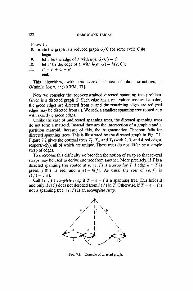
122 GABOW AND TARJAN
Phase II: 8. while the graph is a reduced graph G/C for some cycle C do
begin 9. let e be the edge of F with h(e, G/C) = C;
10. let e’ be the edge of C with h(e’, G) = h(e, G); 11. F: = F + C - e’;
end;
This algorithm, with the correct choice of data structures, is O(min(mlog n, n2)) [CFM, Tl].
Now we consider the root-constrained directed spanning tree problem. Given is a directed graph G. Each edge has a real-valued cost and a color; the green edges are directed from u, and the remaining edges are red (red edges may be directed from u). We seek a smallest spanning tree rooted at u with exactly q green edges.
Unlike the case of undirected spanning trees, the directed spanning trees do not form a matroid. Instead they are the intersection of a graphic and a partition matroid. Because of this, the Augmentation Theorem fails for directed spanning trees. This is illustrated by the directed graph in Fig. 7.1. Figure 7.2 gives the optimal trees T2, T3, and T4 (with 2, 3, and 4 red edges, respectively), all of which are unique. These trees do not differ by a simple swap of edges.
To overcome this difficulty we broaden the notion of swap so that several swaps may be used to derive one tree from another. More precisely, if T is a directed spanning tree rooted at u, (e, f) is a swap for T if edge e E T is green, f 4 T is red, and h(e) = h(f). As usual the cost of (e, f) is c(f) - c(e).
Call (e, f) a complete swap if T - e + f is a spanning tree. This holds if and only if t( f ) does not descend from h ( f ) in T. Otherwise, if T - e + f is not a spanning tree, (e, f) is an incomplete swap.
8
FIG. 7.1. Fmmple of directed graph.

MATROID INTERSECTION PROBLEMS 123
FIG. 7.2. Optimal trees for Fig. 7.1.
Now we give our algorithm for the root-constrained directed spanning tree problem. Let the given cost function be c. Let ~1 = 1 + max{ c(e) - c( f)l e is green, f is red, h(e) = h(f)}. Define a new cost function c’ as follows:
c’(e) = c(e) - p, if e is green,
= c(e), if e is red.
Using cost c’, execute Phase I of Edmonds’ algorithm. This finds a critical tree F in a reduced graph; F contains all the green edges, by choice of c’.
Next execute procedure G, given below, to make swaps until F contains q green edges. Finally, execute Phase II to derive the tree corresponding to F in the original graph.
procedure G; begin
1. while F has more than q green edges do 2. if no swap exists then halt comment the desired tree does
not exist; else begin
3. let (e, f) be a smallest swap; 4. ift(f)doesnotdescendfromh(f)inFthenF:=F-e+f
else begin 5. let C be the cycle formed by f and the path from
h(f) to t(f) in F, 6. reduce C; 7. F:=F-C;
end end end G;
Suppose G is called on the graph of Fig. 7.1 with the cost function shown and q = 3. Figure 7.3 illustrates the swaps done by G. An incomplete swap is illustrated by showing the reduced graph; a complete swap is illustrated by showing the new tree F (in the reduced graph).
Now we show that the algorithm is correct. The desired tree remains the same if the given cost function c is changed by adding a constant to all

124 GABOW AND TARJAN
$ ‘I’
-2 ’ 13’~1 / I ’
/ \
,I \
4
h 7
7 (‘b)
(cl
FIG. 7.3. Swaps done by procedure G. (a) (9,10)-incomplete, (b) (2,4)-incomplete, (c) ( - 2,l)xomplete.
green edges. CalI such a function d. We will exhibit a d such that the following is true:
(1) Every time the algorithm adds a red edge to F, it is critical (for d).
(2) Every reduction is made for a critical cycle (for d).
(3) Every green edge in Fat the end of G is critical (for d) in the final graph.
Using Lemma 7.1, it is easy to show that these conditions imply the algorithm finds a minimum directed spanning tree rooted at u for the cost function d. Also it is clear that the algorithm finds a tree with q green edges. Together these properties show the algorithm is correct.
Now consider the first step of the algorithm, Phase I. d, c, and c’ are identical on the red edges. Thus the first step satisfies (l)-(3). Hence it remains only to show (l)-(3) for procedure G.
We begin by introducing some notation. If b is any cost function, call an edge 6-critical if it is critical when b is the cost function; similarly for a tree or cycle. Let p be the number of iterations of the loop of lines l-7 of G. Let the swaps done by G be (ei, f,), i = 1,. . . ,p. For i = 0, 1,. . . ,p, let G, be the graph at the end of the ith iteration; let ci be the cost function at the end of the i th iteration; if swap ( ei, fi) is incomplete, let Ci be the critical cycle that is reduced. Hence ci is the cost function in Gi: (ei, fi) is a smallest swap for ci-i; if Ci exists then Gi = Gj-,/Ci. (Although cycles Ci are indexed from 1 to p, Ci exists only for incomplete swaps (ei, fi).)

MATROID INTERSECTION PROBLEMS 125
We start by showing the red edges of F are critical with respect to other red edges.
LEMMA 7.2. In graph Gi, let f and g be red edges, with f E F, g 4 F, and h(f)= h(g). Then c,(g) 2 Ci(f)*
Proof. The proof is by induction on i. For i = 0 the Lemma holds because Phase I satisfies (1) and (2) (and d = c on red edges).
For the inductive step, suppose the Lemma holds for Gi-, and consider swap (ei, h). If this swap is complete, line 4 addsfi to F. The Lemma holds for fi, since (ei, fi) is a smallest swap. It continues to hold for other red edges f E F. Hence it holds for all red edges f.
Next suppose (ei, A) is incomplete. In Gi, if f is a red edge of F then h( f, Gi) # Ci, since h(e,, Gi) = C,. By induction the Lemma holds for f. 0
In Figure 7.3 the cost of swaps is increasing. This illustrates the following result.
LEMMA 7.3. The cost of swaps is nondecreasing, i.e., for i = 1,. . . ,p - 1,
Citei+ &+I> 2 Ci-l(ei, L>.
Proof, First suppose (ei, fi) is a complete swap. Line 4 does not create new swaps, nor does it change the cost of existing swaps. The desired inequality follows, since ( ei, h) has smallest cost.
Next suppose (ei, f;) is incomplete. If (e,+i, h,,) is valid before ( ei, f;) is executed, its cost is not changed by lines 5-7 (even if h(f;:+,, Gi -1) E Ci). Again the desired inequality follows. Thus suppose ( ei+ i, fi, i) is not valid before (ei, h). It is easy to see that both h(ei+,, Gipl), h(fi+l, Gi-l) E Ci. Since only one green edge of F has its head in Ci, e,+i = ei. So when Ci is reduced e!, t =fi. Also ci-i(fi::,) < ci-i(fi+J by Lemma 7.2. Thus Ci(fi+l> = Ci-l(fi+l) - Ci-ItfiG-1) 2 0, ad ci(ei+l> = ci-l(ei> - ci-I(&)- So ci(ei+i, fi+t) 2 ci-,(A) - c,-i(ei), which is the desired inequality. q
Lemma 7.3 is the analog of Corollary 3.3 for matroids. As with the latter result, Lemma 7.3 implies that the inequality version of our problem (i.e., finding a smallest spanning tree where the root has degree at least or at most q) can be solved as efficiently as the equality version.
Now we derive the analog of Lemma 7.2 for green edges.
LEMMA 7.4. In graph Gi, let e and g be green edges with e E F, g 4 F, and h(e) = h(g). Then ci(g) 2 ci(e).
Proof. In Gi, if h(e) = h(g) and ci(g) > c,(e), then cj(g) > c,(e) for all j 2 i. This is true because any reduction after the ith iteration decreases

126 GABOW AND TARJAN
the cost of g and e by the same amount. Now it is easy to see that the Lemma follows from this special case: g = ek in a complete swap (ekr fk); C,, i > k, is the first cycle to be reduced that contains h(g, G,); and e = e, in the incomplete swap (ei, h).
Lemma 7.3 shows c, -i(ei, A) >/ ck -i(ek, fk). Thus q(e) = ci-l(ei) - Ci-l(fi) = -Ci-,(e,, J;) G -ckel(ek, fk) = ck-l(g) - ck-l(fk). Note that c,-,(g) = c,-t(g) and ~~-~(f~) = ci-t(fk), by the hypotheses of the spe- cial case. Hence ci( e) 6 ci -1( g) - ci _ i( fk) = ci( g) as desired. 0
NOW we show that the algorithm satisfies properties (I)-(3) with respect to the cost function d defined as follows:
d(g) = c(g) + cp-dep, fp)v if g is green,
= c(g), if gis red.
Define similar functions di, i = 0,. . . ,p, as follows:
di(g) = c,(g) + cp-,(ep,fp), ifgiwm
= ci(g)3 ifgisred.
Suppose the original cost function c is changed to d. It is easy to see that d, is the cost function at the end of Phase I, and di, i = 1,. . . ,p, is the cost function at the end of i th iteration. This follows by induction. (Observe that in a reduction if c(g) changes to c(g) - c(g’), then g’ is in the cycle, hence red, so c( g’) = d( g’).)
Also define Ri, i = 0,. . . , p, as the forest of red edges in Gi that are in F. Now it is easy to see that Lemma 7.5 below is a statement of properties (1) and (2), and Lemma 7.6 is property (3).
LEMMA 7.5. For i = 0 , . . . ,p, Ri is d,-critical in Gi. Further for i = 1,. . . ,p, if swap (ei, fi) is incomplete and contracts cycle Ci, then Ci is d,-,-critical.
Proof. We use induction on i. For the base case, note that F is initially c,-critical and contains all the green edges. Since ca and d, are identical on red edges, R, is de-critical in G,,.
Now suppose 1 < i d p. The ith iteration does swap (ei, A). We start by observing that Ri _ i + f. is di _ ,-critical: Ri _ 1 is di _ ,-critical by induction. Consideredgef;:.Iffisarededgewithh(f)= h(f,),thenciml(f)a cipl(f;) by the choice of (ei, h). Thus di - i( f ) > di _ i( h) as desired. Next suppose e is a green edge with h(e) = h(h). Lemma 7.4 shows c,-i(e) 2 cipl(ei). Lemma 7.3 shows c,-,(e,, f,) > ci-i(ei,fi). Thus dieI = ciel(e) + c,-,(e,, f,) 2 cj-l(ei) + Ci-l(ei, f;) = cipl(fi) = di.-l(fi) as desired.
Now suppose (ei, fi) is a complete swap. Then Rj = RiAl + fi, and di = di -i (since ci = ci-i). Thus the above paragraph shows R; is d+-iti- cal, as desired.

MATROIDINTERSECTIONPROBLEMS 127
Next suppose (ei, fi) is incomplete. The contracted cycle Ci is contained in R,-i + fi and thus is d,-,-critical. It remains to show that Ri is d,-critical. An edge f E Ri is in Ri _ i and does not have its head in Ci (since h ( ei, Gi _ i) E Ci). Hence no costs are modified at vertex h ( f, G, _ i) and f remains critical in Gi. 0
LEMMA 7.6. At the end of procedure G, every green edge of F is d,-critical in Gp.
Proof: Consider a green edge e E F in Gp. If g is a green edge with h(g, G,) = h(e,G,,), then c,(g) > c,(e) by Lemma 7.4, whence d,(g) > d,(e). If f is a red edge with h(f, G,) = h(e, G,), then (e, f) is a swap in GP = GP-i. Since it costs no less than (e,, &.,), c,(e, f) 2 cP(eP, f,). Adding c,(e) to both sides gives d,(f) 2 d,,(e). 0
Since properties (l)-(3) are established, the algorithm is correct. (It is easy to see that if procedure G halts in line 2, there is no spanning tree rooted at u with q green edges.)
It is not difficult to implement the algorithm in time O(min(m log n, n*)) using the data structures of [Tl, CFM]. This involves using one UNION-FIND structure to represent vertices of the reduced graph, another to represent trees in the forest F, and priority queues to keep track of the costs of all edges with a given head [Tl]. The cycles are represented by a tree structure [CFM]. In addition, procedure G uses a priority queue of swaps (for line 3).
THEOREM 7.1. A smallest root-constrained directed spanning tree can be found in time O(min(m log n, n*)) and space O(m + n).
Proof. Correctness follows from Lemmas 7.1-7.6 and the accompanying discussion. Further details concerning the time bound are left to the reader. 0
We conclude this section with a lower bound for our approach. Say that an algorithm on a directed graph “uses the swap sequence approach” if, given a graph as shown in Fig. 7.4a, it determines the complete swaps found by procedure G (with q = n). Note that the algorithm need not determine the incomplete swaps; as usual the algorithm need not determine the order of the complete swaps. Also, although swaps may be for reduced graphs, they are specified by the edges of the original graph.
LEMMA 7.7. Any algorithm on a directed graph that uses the swap sequence approach requires Q(sort( n)) time.
Proof: As in Lemma 4.1 we show that with only O(n) extra processing, the algorithm, called on an n + 2 vertex graph, can sort n numbers.
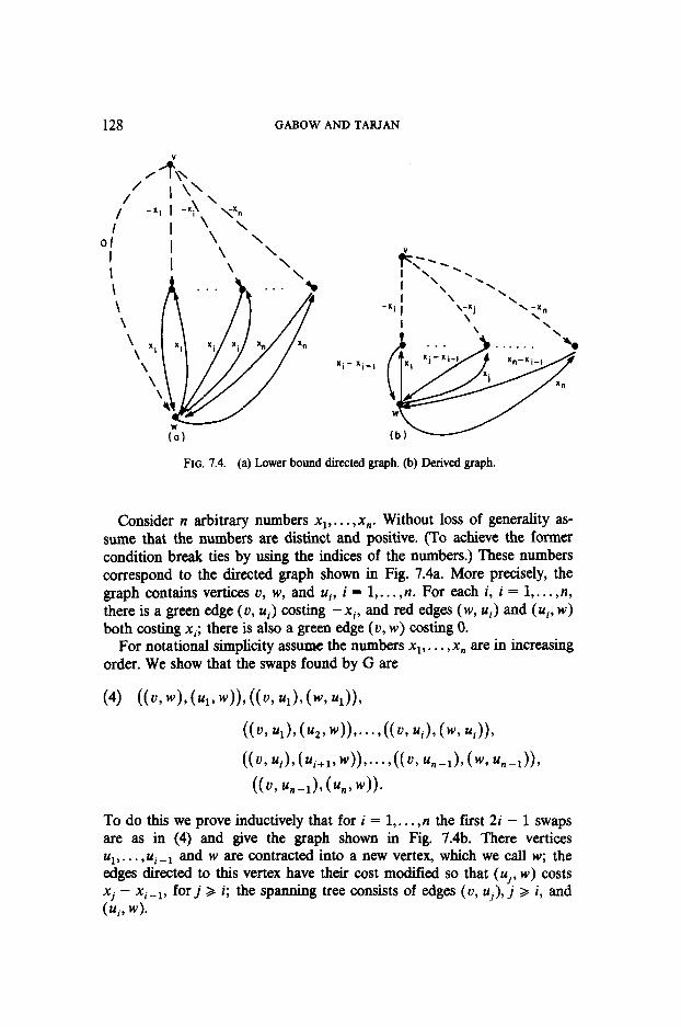
128 GABOW AND TARJAN
/ /&
,I -XI I \‘,
I I 4, \;“”
Ol ’ \‘\ I
I I ‘\ ‘1,
\ . . . . . . %
\
\
\
\ XI 3
w
xi xi x, %I
\
\ \
N
w (0)
xi- xi-)
I \ \ \
FIG. 7.4. (a) Lower bound directed graph. (b) Derived graph.
Consider n arbitrary numbers x1,. . . ,x”. Without loss of generality as- sume that the numbers are distinct and positive. (To achieve the former condition break ties by using the indices of the numbers.) These numbers correspond to the directed graph shown in Fig. 7.4a. More precisely, the graph contains vertices u, w, and ui, i = 1,. . . ,n. For each i, i = 1,. . . ,n, there is a green edge (u, ui) costing -xi, and red edges (w, ui) and (ui, w) both costing xi; there is also a green edge (u, w) costing 0.
For notational simplicity assume the numbers x1,. . . ,x, are in increasing order. We show that the swaps found by G are
(4) ((4 4, h WI), (GA Ul), 6% 4)9
t(“~ul)~(u*~w))~~‘~~((u~ ui),(w9 ui))9
((u9 ~i)‘(ui+l,w)),...,((u, %-MY u,-I)),
((h %-113 (U”9 4).
To do this we prove inductively that for i = 1,. . . ,n the first 2i - 1 swaps are as in (4) and give the graph shown in Fig. 7.4b. There vertices Ul,..., ui _ r and w are contracted into a new vertex, which we call w; the edges directed to this vertex have their cost modified so that (ui, w) costs
- xi-r, for j > i; the spanning tree consists of edges (u, uj), j > i, and ;:, w).
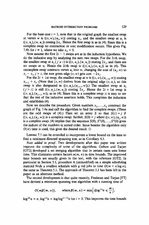
MATROID INTERSECTION PROBLEMS 129
For the base case i = 1, note that in the original graph the smallest swap at vertex w is ((u, w), (ui, w)) costing x1, and the smallest swap at ui is ((u, ui), (w, ui)) costing 2xi. Hence the first swap is as in (4). Since this is a complete swap no contraction or cost modification occurs. This gives Fig. 7.4b for i = 1, where we take x0 = 0.
Now assume the first 2i - 1 swaps are as in the induction hypothesis. We do the inductive step by analyzing the next two swaps. For the 2ith swap, the smallest swap at uj (i >/ i) is ((u, ui), (w, uj)) costing 2xj, and there are no swaps at y. Hence the 2ith swap is ((u, ui), (w, ui)) as in (4). This incomplete swab contracts vertex ui into w, changing the cost of (uj, w) to xj - xi, j > i; the new green edge (u, w) gets cost - 2xi.
For the 2i + 1st swap, the smallest swap at w is ((u, w), ( ui+ i, w)) costing xi+i + xi. (Note that (u, w) derives from the original edge (u, ui), so this swap is also designated as ((u, ui),(ui+i, w)).) The smallest swap at yj (j > i) is still ((u, uj), (w, uj)) costing 2xj. Hence the 2i + 1st swap is (t”, Ui),(Ui+19 w)), as in (4). Since this is a complete swap it is easy to see that the rest of the inductive assertion holds. This completes the induction and establishes (4).
Now we describe the procedure. Given numbers xi,. . . ,x, construct the graph of Fig. 7.4a and call the algorithm to find the complete swaps. (These are the odd swaps of (4).) Then set an array S so that S(i) = j if ((u, ui), ( uj, w)) is a complete swap; further, S(0) = j where ((u, w), ( uj, w)) is a complete swap. (4) implies that the sequence S(O), S*(O), . . . ,P(O) gives the indices of the numbers in sorted order. Since besides the algorithm only O(n) time is used, this gives the desired result. q
Lemma 7.7 can be extended to incorporate a lower bound on the time to find a minimum directed spanning tree, as in Corollary 4.1.
Note added in proof. Two developments after this paper was written improve the complexity of some of the algorithms. Gabow and Tarjan [GT2] developed a set merging algorithm that in certain cases uses linear time. This eliminates certain factors a(m, n) in time bounds. The improved time bounds are usually given in the text, with the reference [GT2]. In particular in Section 5.1, procedure A (unmodified) on a simple scheduling matroid finds a smallest schedule with q red jobs in time O(m + n log n), the same as Theorem 5.1. The approach of Theorem 5.1 has been left in the paper as an alternate method.
The second development is that quite recently, Fredman and Tarjan [FT] have devised a minimum spanning tree algorithm with a running time of
OWh n))7 wherep(m, n) = min{ i(log(‘)n < x),
log’% = n, log% = log log ciV1)n for i > 0. This improves the time bounds

130 GABOW AND TARJAN
in Section 4: For Theorem 4.1, the time to find a smallest spanning forest with q red edges is U( m + n log n). For Theorem 4.2, the time to find a smallest spanning tree with a degree constraint is O( m /3( m, n)).
REFERENCES
[AHU] A. AHO, J. HOPCROFT, AND J. ULLMAN, “The Design and Analysis of Computer Algorithms”, Addison-Wesley, Reading, Mass., 1974.
PI T. H. BRYLAWSKI, Some properties of basic families of subsets, Discrete Math. 6 (1973), 333-341.
[BFPRT] M. BLUM, R. FLOYD, V. PRATT, R. RIVEST, AND R. TARJAN, Time bounds for
PM1
WI
[El [EW
IFI
WI IGall
OQl
[GKI
WI
W-11
[G-t-A
[GUI
WI
[Jl
[JMI
WI
selection, J. Comput. System Sci. 7 (1973), 448-461. P. M. CAMERINI, L. FRAITA, AND F. MAFFIOLI, A note on finding optimum branchings, Networks 9 (1979), 309-312. D. CHERITON AND R. E. TARJAN, Finding minimum spanning trees, SZAM J.
Comput. 5 (1976), 724-741. J. EDMONDS, Optimum branchings, J. Res. Nat. Bur. Standards 71B (1967), 233-240. P. VAN EMDE BOAS, R. KAAS, AND E. ZIJLSTRA, Design and implementation of an efficient priority queue, Math. Systems Theory 10 (1977), 99-127. N. FRIEDMAN, Some results on the effect of arithmetics on comparison problems, in “Proceedings, 13th Annual Symposium on Switching and Automata Theory, College Park, Md., 1972,” pp. 139-143. M. FREDMAN AND R. TARJAN, Fibonacai leaps and their uses, to appear. H. N. GABOW, A good algorithm for smallest spanning trees with a degree con- straint, Networks 8 (1978), 201-208. H. N. GABOW, An efficient implementation of Edmonds’ algorithm for maximum matching-on graphs, J. Assoc. Comput. Mach. 23 (1976), 221-234. F. GLOVER AND D. KL.INGMAN, Finding minimum spanning trees with a fixed number of links at a node, in “Combinatorial Programming: Methods and Applica- tions,” (B. Roy, Ed.), pp. 191-200, Reidel Publishing, 1975. F. GLOVER, Maximum matching in a convex bipartite graph, Naval Res. Logist. Quart. 14 (1967), 313-316. H. N. GABOW AND R. E. TARIAN, Efficient algorithms for simple matroid intersec- tion problems, in “Proceedings, 20th Annual Symposium on Foundations of Com- puter Science, San Juan, Puerto Rico, 1979,” pp. 196-204. H. N. GABOW AND R. E. TARIAN, A linear-time algorithm for a special case of disjoint set union, in “Proceedings 15th Annual ACM Symposium on Theory of Camp.,” 1983, 246-251. D. GUSFIELD, Matroid optimization with the interleaving of two ordered sets, in “Proceedings of the Humboldt Conference on Graph Theory, Combinatories and Computing,” 1979, Utilities Mathematics; also Discrete Appl. Math., to appear. E. HOROWITZ AND S. SAHNI, “Fundamentals of Computer Algorithms,” Computer Science Press, Potomac, Md., 1978. J. R. JACKSON, “Scheduling a Production Line to Minimize Maximum Tardiness,” Research Rep. 43, Management Science Research Project, University of California, Los Angeles, 1955. D. B. JOHNSON AND T. MIZOGUCHI, Selecting the Kth element in X + Y and X, + X2 . + X,, SIAM J. Comput. 7 (1978), 147-153. R. M. KARP, A simple derivation of Edmonds’ algorithm for optimum branchings, Networkr 1 (1971), 265-272.

MATROID INTERSECTION PROBLEMS 131
PI
u-21 V-F1
[LPI
PI
Fl
WI
[sppl
WI
WI P-4
WI
WI WI
E. L. LAWLER, “Combinatorial Optimization: Networks and Matroids,” Holt, Rinehart&Winston, New York, 1976. E. L. LAWLER, Matroid intersection algorithms, Math. Programming 9 (1975), 31-56.
T. LANG AND E. B. FERNANDEZ, Scheduling of unit-length independent tasks with execution constraints, Inform. Process. Left. 4 (1976), 95-98. W. LIPSKI, JR., AND F. P. PREPARATA, Efficient algorithms for finding maximum matchings in convex bipartite graphs and related problems, Actu Informatica 15 (1981), 329-346. C. PAPADIMITRIOU, The complexity of the capacitated tree problem, Networks 8 (1978), 217-230. M. I. SHAMOS, Geometry and statistics: Problems at the interface, in “Algorithms and Complexity: New Directions and Recent Results,” (J. F. Traub, Ed.), pp. 251-280, Academic Press, New York, 1976. P. M. SPIRA AND A. PAN, On finding and updating spanning trees and shortest paths, SIAM J. Comput. 4 (1975), 375-380. A. SCH~NHAGE, M. PATERSON, AND N. PIPPENGER, Finding the median, J. Comput. @tern Sci. 13 (1976), 184-199. D. SLEATOR AND R. E. TARJAN, A data structure for dynamic trees, J. Comput. System Sci. 26 (1983), 362-391. R. E. TARIAN, Finding optimum branchings, Networks 7 (1977), 25-35. R. E. TARTAN, “Data Structures and Network Algorithms,” Society for Industrial and Applied Mathematics, Philadelphia, Penn., 1983. R. A. UBELMESSER, “Finding Smallest Spanning Trees with One Degree Constraint,” M. S. thesis, Department of Computer Science, University of Colorado, Boulder, 1978. D. J. A. WELSH, “Matroid Theory,” Academic Press, New York, 1976. A. C. YAO, An O(IEllogloglVI algorithm for finding minimum spanning trees, Inform. Process. Lett. 4 (1975), 21-23.


![Weighted Linear Matroid Parity - University of Toronto · 2012. 6. 28. · Satoru Iwata (RIMS, Kyoto University) Extensions of Matching and Matroids •Matroid Parity [Matroid Matching]](https://img.pdfslide.net/doc/110x75/613ac999f8f21c0c8268a299/weighted-linear-matroid-parity-university-of-toronto-2012-6-28-satoru-iwata.jpg)