Embed Size (px)
Citation preview
Efficient and accurate methods for
computational simulation of netting
structures with mesh resistance
to opening
Amelia de la Prada Arquer
DOCTORAL THESIS
Advisor: Manuel González Castro
Programa Oficial de Doctorado en Ingeniería Industrial
Ferrol, July 2014


A mi familia:
Florian, Amelia y Manuel
To my family:
Florian, Amelia y Manuel


i
Aknowledgements This Ph.D. thesis has been conducted at the Mechanical Engineering
Laboratory of University of A Coruña, headed by Prof. Javier Cuadrado. This
research was motivated by the project PSE-REDES, Subproject 3, Simulation,
experimentation and design of fishing gears, supported by the Spanish Ministry of
Science and Innovation.
First, I wish to express my special gratitude to Prof. Manuel González, my
advisor, for his excellent advice, dedication, patience, and the passion for research
and well-finished work he has transmitted to me. Also, I would like to thank to Prof.
Javier Cuadrado, for giving me such a great opportunity.
I would like to thank my colleagues at the Mechanical Engineering
Laboratory: Alberto, Daniel, David, Emilio, Florian, Fran, Miguel, Roland and
Urbano. For the fabulous work environment they have provided, their useful advice
and the enjoyable hours we have spent together.
During my doctorate, I have made a stay at the IFREMER at Brest, under the
supervision of Daniel Priour. I am grateful for his kindness and the very interesting
and productive conversations that helped me to better understand the fishing nets’
behaviour. Also, many thanks to his research team for welcoming me so warmly.
Finally, I owe my heartfelt thanks to my close people: to my parents, for
supporting me despite the distance that separates us; and last but no least to my
husband, Florian, for his love and support, which always encourage me to give the
best of myself.

ii

iii
Agradecimientos Esta tesis doctoral ha sido realizada en el Laboratorio de Ingeniería Mecánica
de la Universidad de A Coruña, dirigido por el profesor Javier Cuadrado. Esta
investigación fue motivada por el proyecto PSE-REDES, Subproyecto 3, Simulación,
experimentación and rediseño de artes y dispositivos de pesca, financiado por el
Ministerio de Ciencia e Innovación de España.
En primer lugar, me gustaría dar las gracias al profesor Manuel González, mi
director de tesis, por sus excelentes consejos, dedicación, paciencia y la pasión por la
investigación y el trabajo bien hecho que ha sabido trasmitirme. También agradecer
al profesor Javier Cuadrado, por haberme brindado esta gran oportunidad.
Quiero dar las gracias a mis compañeros del Laboratorio de Ingeniería
Mecánica: Alberto, Daniel, David, Emilio, Florian, Fran, Miguel, Roland and
Urbano, por el fabuloso ambiente de trabajo, sus utilísimos consejos y las agradables
horas que hemos pasado juntos.
Durante mi doctorado he realizado una estancia en el IFREMER en Brest,
bajo la supervisión de Daniel Priour. Le estoy muy agradecida por su amabilidad y
las interesantes conversaciones que me ayudaron a entender mejor el
comportamiento de las redes de pesca. Me gustaría agradecer también a su equipo de
investigación, por haberme proporcionado una acogida tan cálida.
Finalmente, me gustaría dar las gracias a aquellas personas que siempre han
estado a mi lado, a mis padres, por su cariño y apoyo a pesar de la distancia que nos
separa y, por último, a mi esposo Florian, por su amor y apoyo que siempre me
impulsan a dar lo mejor de mí.

iv
v
Abstract Current research in computational simulation of fishing gears focuses on
efficient numerical models that accurately predict the behaviour of the netting
structure. This thesis is collection of four papers related to the development of a new
model that includes the mesh resistance to opening.
Firstly, several nonlinear stiffness models of a net twine are developed. The
net twine is modelled as a double-clamped beam and its force-displacement response
is calculated by finite element analysis and approximated with three different
models. The proposed models overcome the drawbacks of previous models. The
twine model is based on the bending stiffness and other geometrical properties of the
netting material, so, a procedure to quantify them is presented. Although the
methodology is similar to the previous studies, several original contributions are
introduced, like a simpler experimental set-up. This procedure is also used to validate
the presented twine models with experimental data.
Regarding the simulation, the performance of a fishing gear is mainly
determined by its equilibrium shape. In this thesis, the robustness and efficiency of
gradient-based energy minimization methods and Newton iteration are compared by
applying them to a set of benchmark problems.
Finally, a lumped mass formulation for netting structures is developed. The
lumped mass formulation is widely used to model netting structures, but in this thesis
the linear springs that traditionally connect the nodes are replaced by the developed
twine model. Besides, the knots are modeled as spheres instead of point masses.
Although the expressions of the presented model are more complex than those of the
spring model, it has been demonstrated that both models have a similar
computational overhead. To validate the model, a netting panel is simulated and
compared with experimental results.

vi

vii
Resumen La investigación actual en simulación computacional de artes de pesca se
centra en modelos numéricos eficientes capaces de predecir con precisión el
comportamiento del material de la red. Esta tesis es un compendio de artículos
relativos al desarrollo de un nuevo modelo que incluye la resistencia a la apertura.
En primer lugar, se desarrollan varios modelos de rigidez no lineal para un
hilo de red. El hilo es modelado como una viga biempotrada y su respuesta fuerza-
desplazamiento es calculada mediante análisis por elementos finitos y aproximada
por tres modelos diferentes. Se obtienen diferentes variantes en función de la
expresión utilizada para aproximar dicha respuesta. El modelo propuesto supera las
desventajas de los modelos previos. El modelo está basado en la rigidez a flexión,
por tanto, se presenta también un procedimiento para cuantificarla. Aunque la
metodología es similar a la de estudios previos, en esta tesis se aportan nuevas
contribuciones, como un montaje experimental más simple.
En cuanto a la simulación, el funcionamiento de un arte de pesca viene
determinado principalmente por su posición de equilibrio. En esta tesis se comparan
la robustez y eficiencia de los métodos de minimización de energía basados en el
gradiente y del método de Newton-Raphson, aplicándolos a un conjunto de
problemas representativos.
Finalmente, se desarrolla una formulación basada en masas suspendidas para
modelar la red. La formulación de masas suspendidas es ampliamente utilizada para
modelar la red, pero en esta tesis los muelles que tradicionalmente conectan los
nodos son remplazados por el modelo de hilo propuesto. Además, los nudos de la red
son modelados como esferas en lugar de masas puntuales. Aunque las expresiones
del modelo propuesto son más complejas que las de los muelles, se demuestra que
ambos modelos tienen un coste computacional similar. Para validar el modelo, un
paño de red es simulado y comparado con resultados experimentales.

viii
ix
Resumo A investigación actual en simulación computacional de redes de pesca
céntrase en modelos numéricos eficientes, capaces de prever con precisión o
comportamento da estructura da rede. Esta tese é un compendio de artigos sobre o
desenvolvemento dun novo modelo que inclúe a resistencia á abertura.
En primeiro lugar, desenvólvense varios modelos de rixidez non lineal para
fíos de redes. O fío é modelado como unha viga biempotrada e a súa resposta de
forza-desprazamento foi calculada mediante análise de elementos finitos e
aproximada mediante diferentes modelos. O modelo proposto supera as desvantaxes
dos modelos anteriores. O modelo baséase na rixidez a flexión, e polo tanto, tamén se
presenta un novo método para cuantificala. Aínda que a metodoloxía é semellante á
de estudos anteriores, o novo método ten importantes vantaxas, como por exemplo
unha configuración experimental máis simple.
Con respecto á simulación, compárase a robustez e eficiencia de dúas familias
de métodos para calcular a posición de equilibrio: métodos de minimización
baseados no gradiente e método de Newton-Raphson, aplicándose a un conxunto de
problemas representativos.
Por último, desenvólvese unha nova formulación de masas suspendidas para
estruturas de rede. A formulación de masa suspendida é amplamente utilizada para
modelar a rede, pero nesta tese os resortes que tradicionalmente conectando os nodos
son reemplazados polo modelo desenvolvido nesta tese. Ademais, os nós da rede son
modelados como esferas, en vez de masas puntuais. Aínda que as ecuacións do
modelo proposto son máis complexas do que as resortes, móstrase que ambos
modelos posúen un custo computacional similar. Para validar o modelo, un pano de
rede é simulado e comparado cos resultados experimentais.

x
xi
Resumen extendido
Motivación
La conservación de los recursos marinos es fundamental para suministrar
alimentos a la población mundial y garantizar la sostenibilidad del sector pesquero
como un medio de vida. La FAO (Food and Agriculture Organization of the United
Nations) estima que unos 3 mil millones de personas dependen del pescado como su
principal fuente de proteína animal (FAO, 2012). Sin embargo, la contaminación, la
sobreexplotación y la destrucción de los hábitats marinos están amenazando el futuro
de este sector. Por ello, la Unión Europea está haciendo grandes esfuerzos políticos
para garantizar su continuidad.
Una de las estrategias a seguir es mejorar el diseño de artes de pesca para
reducir su impacto medioambiental e incrementar su eficiencia energética. Estos
objetivos están directamente relacionados con la forma que toma la red ante un flujo
de corriente, esto es, su comportamiento estructural e hidrodinámico (Suuronen,
2005). Dicho comportamiento depende de muchos factores: la geometría de la red
(forma, tamaño y configuración de las mallas, presencia de elementos rígidos y
flexibles, cables, etc.), condiciones de trabajo (velocidad de arrastre, tipo de suelo
marino, olas, condiciones climáticas, etc.) y peso y volumen de la captura. Entender
y predecir la influencia de estos factores es crítico para mejorar los nuevos diseños.
El método tradicional para comprobar el funcionamiento de un arte de pesca
consiste en campañas experimentales, que son enormemente costosas y lentas. Como
alternativa más barata, se utilizan los ensayos en canal hidrodinámico, aun así, estos
ensayos siguen siendo lentos y caros porque, además del coste de alquiler de las
instalaciones, los ensayos se realizan con prototipos escalados del arte. Además, no
permiten reproducir las condiciones de trabajo reales (olas, corrientes variables,
suelo marino, etc.). Los inconvenientes de estos ensayos han impulsado el desarrollo
de modelos numéricos para predecir la forma del arte, no obstante, la validación de
éstos modelos con ensayos experimentales es siempre necesaria.

xii
La presente tesis doctoral es un compendio de cuatro artículos enfocados al
modelado y simulación de redes, con el objetivo de desarrollar un modelo numérico
robusto y eficiente computacionalmente, capaz de predecir con exactitud el
comportamiento real de la red, pudiendo resolver algunos de los inconvenientes de
los modelos previos.
Resistencia a la apertura de mallas
En un paño de red, el hilo se anuda formando un conjunto de mallas, cuya
configuración puede ser tipo diamante (la más común), hexagonal o cuadrada. Uno
de los rasgos más relevantes de las mallas es la resistencia a la apertura, puesto que
ésta es crucial para alcanzar uno de los objetivos relativos a reducir el impacto
medioambiental de un arte de pesca, la selectividad.
La selectividad se define como la capacidad para capturar especies objetivo y
dejar a las otras escapar. Se ha demostrado que la selectividad depende
principalmente de la resistencia a la apertura debido a que ésta limita la apertura de
las mallas en el copo, impidiendo que los peces de talla pequeña escapen (Herrmann,
B., 2006; Sala, A., 2007b). La mayoría de los modelos numéricos para redes ignoran
la resistencia a la apertura porque asumen que los hilos son completamente flexibles
y flectan sin resistencia. Sin embargo, en los últimos años crece la tendencia a
utilizar hilos más gruesos y fuertes en la fabricación de copos de red ya que así
aumenta su durabilidad, afectando negativamente a la selectividad al incrementar la
resistencia a la apertura de las mallas. Por lo tanto, la incorporación de la resistencia
a la apertura a los modelos numéricos es esencial para poder predecir con precisión
el comportamiento de la red.
En mallas tipo diamante, la resistencia a la apertura se caracteriza por la
rigidez a flexión EI del hilo (Herrmann, B., 2006; O’Neill, 2004). Entonces, el
principal reto es el desarrollo de un modelo de resistencia a la apertura que esté
basado en esta propiedad. La investigación más relevante sobre rigidez a flexión ha
sido desarrollada por O’ Neill (2002); él describió las ecuaciones que gobiernan la
flexión en un hilo basándose en la teoría de vigas, encontrando dos soluciones
analíticas para ellas (una solución exacta y una solución asintótica aproximada).
Aunque estas soluciones analíticas son muy apropiadas para describir la flexión en el
xiii
hilo (O’Neill and Priour, 2009; Sala et al., 2007a), presentan dos inconvenientes
importantes a la hora de aplicarlas a la simulación numérica de redes: su alto coste
computacional y que no tienen en cuenta los esfuerzos axiales, al considerar el hilo
inextensible.
Puesto que los modelos presentados dependen de la rigidez a flexión, la
medida de esta propiedad mecánica es indispensable. La investigación más relevante
ha sido desarrollada por Sala (2007a), pero ésta requiere un instrumento de medida
especialmente diseñado para medir deformaciones en un paño de red, que no está
disponible en el mercado. Además, los autores remarcaron la falta de ajuste entre los
datos experimentales y el modelo numérico (utilizaron la solución asintótica de
O’Neill (2002)).
Por lo tanto, los objetivos de la presente tesis, en cuento a la resistencia a la
apertura son:
1) Desarrollar un modelo de hilo que supere las desventajas explicadas
anteriormente. El modelo debe representar de forma correcta el
comportamiento a flexión de un hilo, y ser robusto y eficiente desde el punto
de vista computacional, puesto que va orientado a la simulación de artes de
pesca reales, que pueden estar formados por un gran número de variables.
2) Desarrollar un montaje experimental que permita analizar datos para estimar
la resistencia a la apertura de forma más simple y precisa que el método
propuesto por Sala et al. (2007a).
Los artículos asociados a esta investigación son los artículos No.1 y No. 2:
El artículo No.1 comprende el primer objetivo de esta tesis. En él, se presenta
un nuevo modelo de hilo a flexión, el cual trata de resolver los inconvenientes de los
modelos desarrollados por O’Neill (2002). El segundo artículo corresponde al
segundo objetivo, donde se describe un procedimiento experimental para medir la
rigidez a flexión y otros parámetros geométricos para diferentes materiales de red.

xiv
Equilibrio estático de redes
En lo que respecta a la simulación, en la mayoría de aplicaciones marítimas,
el funcionamiento de un arte de pesca viene determinado, principalmente por su
posición de equilibrio bajo condiciones estáticas o quasi-estáticas, esto es, su
posición de equilibrio sometido a una corriente de agua constante (Priour, 1999;
Priour et al., 2009; O’Neill and Priour, 2009). Se trata de resolver el sistema de
ecuaciones formado por todas las fuerzas que actúan en el arte de pesca, por ejemplo,
las fuerzas elásticas, derivadas de los modelos de la red (como los descritos
anteriormente) y cables, las fuerzas hidrodinámicas, contacto con el fondo marino,
peso y flotación, etc. Algunas de estas fuerzas introducen ecuaciones altamente no
lineales en el sistema, esto hace la aplicación de algoritmos iterativos necesaria para
resolver el problema.
Uno de los métodos más comunes para resolver sistemas de ecuaciones no
lineales es el método de Newton-Raphson, aunque ha sido ya utilizado con éxito,
presenta dos desventajas principales: la primera es la dificultad de implementación
del método, puesto que requiere la matriz Jacobiana de las fuerzas descritas
anteriormente; la segunda es que la matriz Jacobiana puede presentar problemas de
mal condicionamiento a lo largo de las iteraciones. Como alternativa al método de
Newton-Raphson, en esta tesis se propone el uso de métodos de minimización de
energía basados en el gradiente.
En cuanto a la implementación del modelo, es necesaria una formulación
basada en el modelo de hilo mencionado anteriormente. Una de las formulaciones
más utilizadas es la formulación basada en masas suspendidas (Bessoneau, J.S. and
Marichal, D. 1998; Le Dret et al. 2004; Lee et al., 2005; Li et al., 2006; Takagi et al.,
2004; Theret, F., 1993), ésta consiste en una serie de masas puntuales (que
representan los nudos de la red) interconectadas por muelles lineales (que
representan los hilos). Las formulaciones de masas suspendidas desarrolladas hasta
ahora presentan dos inconvenientes principales: (i) la aproximación de los hilos
como muelles lineales y (ii) no tienen en cuenta el tamaño de los nodos de red.
Además, como los muelles no representan el comportamiento real del muelle, se
suelen añadir nodos intermedios para mejorar la precisión del modelo, lo cual
incrementa el coste computacional.
xv
Por tanto, los objetivos de la tesis son:
3) Encontrar el método más apropiado para resolver la posición de equilibro de
la red con el objetivo de solventar las desventajas del método de Newton-
Raphson.
4) Desarrollar un modelo de red basado en la formulación de masas suspendidas
y el modelo de hilo del artículo No. 1, teniendo en cuenta el tamaño de los
nudos. El modelo debe ser validado comparando los resultados numéricos
con datos experimentales.
Los artículos de esta tesis relacionados con estos objetivos son los artículos
No. 3 y No. 4:
Aunque encontrar el método más apropiado para simular la red (el tercer
objetivo de esta tesis) es una tarea intermedia para simular el modelo propuesto, el
artículo No. 3 consiste en un estudio detallado sobre éste objetivo. Es un análisis de
la robustez y la eficiencia computacional de dos familias de métodos: el método de
Newton-Raphson (NR) y métodos de minimización de energía basados en el
gradiente, con el objetivo de analizar sus ventajas e inconvenientes y cómo les
afectan distintas características de la red.
El artículo No. 4 comprende el cuarto objetivo, usando los artículos
mencionados anteriormente para alcanzarlo: el modelo de hilo del artículo No. 1 es
incorporado a la formulación de masas suspendidas. Para encontrar su posición de
equilibrio, se utiliza el método basado en el gradiente propuesto en el artículo No. 3.
Finalmente, se utiliza el experimento presentado en el artículo No. 2 para validar el
modelo.
Resultados
Los modelos de hilo propuestos (modelo de ajuste polinómico de las fuerzas,
y modelo de ajuste por splines de la energía potencial del artículo No.1) cumplen con
éxito los objetivos planteados. Los modelos coinciden con la solución obtenida
mediante análisis por elementos de una viga a flexión en el artículo No. 1. Aunque
los modelos no son igualmente precisos, los errores relativos a la solución de
referencia son aceptables, ajustándose perfectamente a los resultados experimentales,

xvi
tanto en la validación experimental del modelo en el artículo No. 1 como en las
estimaciones de la rigidez a flexión en el artículo No. 2, con un coeficiente de
determinación comprendido entre 0.97 y 0.99 para todos las muestras de paños de
red ensayadas.
Además, se han implementado también las soluciones asintótica y exacta
desarrolladas por O’Neill (2002), para compararlas con los modelos propuestos. Sus
diferencias pueden apreciarse en el test del artículo No. 1 mencionado anteriormente.
La solución exacta coincide con la referencia hasta que la deformación vertical es
muy alta, lo mismo ocurre con la solución asintótica la explicación para este
fenómeno es que O’Neill no tuvo en cuenta la deformación axial. Además, la
solución asintótica presenta diferencias más pronunciadas respecto a la solución de
elementos finitos. Estas diferencias tienen un impacto negativo en el ajuste con los
datos experimentales; el peor ajuste en el artículo No. 1 se corresponde con el de la
solución asintótica y en el artículo No. 2 generó problemas en la estimación de
parámetros, coincidiendo con las observaciones de Sala et al. (2007a). Por el
contrario, la solución exacta generó ajustes muy precisos en ambos artículos. La
solución exacta representa con éxito el comportamiento del hilo, sin embargo, lo
hace bajo un alto coste computacional y una difícil implementación. Los nuevos
modelos propuestos son una alternativa a la solución exacta, puesto que sus
ecuaciones son mucho más simples y eficientes pero la calidad del ajuste con los
datos experimentales es muy similar.
En cuanto al montaje experimental, en este trabajo se propone una alternativa
más simple que el utilizado por Sala et al. (2007a). Aunque el montaje se describe en
detalle en el artículo No. 2, los resultados experimentales se utilizan en más artículos
con diferentes propósitos: en el artículo No.1 se utilizan para validar el modelo de
hilo, y en el artículo No. 4 vara validar el modelo de red, particularizado para las
dimensiones de la muestra de red.
El procedimiento propuesto en el artículo No. 2 proporciona estimaciones
para la rigidez a flexión y otros parámetros geométricos a partir de datos
experimentales. Se han analizado dos modelos de hilo desarrollados en (O’Neill,
2002) y otros dos modelos de hilo ya estudiados en el artículo No. 1 combinados con
cuatro estrategias diferentes de restricción de parámetros. Se ha demostrado que el
xvii
método propuesto es una forma simple y eficiente para estimar la resistencia a la
apertura de redes. No obstante, hay que tener en cuenta que las estimaciones no son
valores reales absolutos de las propiedades de la red, sino parámetros de calibración
de los diferentes modelos. Por tanto, el modelo utilizado para estimar los parámetros
debe ser el mismo que el que se aplicará para predecir el comportamiento de la red.
Sin embargo, este método presenta algunas objeciones que requieren
investigaciones futuras: en primer lugar, este método no permite estimar la altura del
nodo; segundo, no tiene en cuenta la flexión fuera del plano de la red, la cual puede
influir en la resistencia a la apertura. Además, en el artículo No. 2, se ha demostrado
que la resistencia a la apertura es diferente en los ciclos de carga y descarga,
probablemente causada por deformaciones plásticas en el material debido a que
estuvo expuesto a altas tensiones durante largo tiempo. Estos resultados sugieren que
son necesarias investigaciones futuras para analizar cómo el historial de carga afecta
a la resistencia a la apertura durante el uso de los artes de pesca.
En lo que respecta al análisis de métodos para la simulación de redes, los
resultados muestran que el método de minimización de energía basado en el
gradiente más adecuado es el método de memoria limitada BFGS (LBFGS). Por otro
lado, la mejor variante de la familia de NR es el método NR de paso limitado
(propuesto por los autores). Ambos métodos tienen sus ventajas e inconvenientes y el
uso de uno u otro viene indicado por la situación. Por un lado LBFGS es más robusto
y eficiente en problemas donde la posición inicial está lejos de la solución, por
ejemplo, cuando ésta es muy difícil de estimar, como en redes compuestas por
paneles diferentes. Por otro lado NR es más rápido cuando la posición inicial está
muy cerca de la posición de equilibrio, por ejemplo, cuando las condiciones de
simulación son levemente modificadas respecto a la situación anterior, como en las
aplicaciones de optimización automática de la topología de la red (Khaled et al.,
2012; Priour, 2009). De hecho, ambos métodos pueden incluso combinarse,
utilizando LBFGS en las primeras iteraciones para acercar la posición inicial al
equilibrio y después aplicar NR para aumentar la precisión de los resultados. En
cuanto a la implementación de los métodos, LBFGS es mucho más fácil de
implementar, puesto que no requiere la matriz Jacobiana.
xviii
En el artículo No. 4, el método LBFGS es utilizado para calcular la posición
de equilibrio de una red modelada con una formulación que incluye la resistencia a la
apertura. El modelo propuesto se basa en la formulación de masas suspendidas, pero
los muelles lineales que tradicionalmente conectan los nodos son reemplazados por
el modelo de hilo de ajuste polinómico de la fuerza descrito en el artículo No. 1.
Además, los nodos de la red son aproximados como esferas en lugar de masas
puntuales. Para validar el modelo, los datos experimentales del artículo No. 2 son
analizados con el modelo propuesto como función modelo en la regresión,
particularizado para el paño de red utilizado en los experimentos. La bondad del
ajuste confirma que el modelo es capaz de predecir la resistencia a la apertura. Dado
que el modelo de hilo ya ha sido validado en el artículo No. 1, en este caso los
sujetos de validación son: la aproximación de la geometría del paño de red mediante
la formulación de masas suspendidas y la hipótesis de nodos esféricos. En cuanto a la
eficiencia computacional, aunque pueda parecer que la incorporación del modelo de
hilo a la red incrementa su coste computacional porque requiere la evaluación de
raíces y funciones trigonométricas, se ha demostrado lo contrario. Un experimento
numérico se ha llevado a cabo para comparar su eficiencia computacional con el
modelo tradicional de masas suspendidas, los resultados muestran que aunque el
tiempo por evaluación de función por nodo del modelo propuesto es más alto, no es
necesario incluir los nodos intermedios del modelo tradicional, resultando en un
coste computacional total similar.
Conclusiones
Esta tesis aspira a desarrollar nuevos modelos de hilo eficientes y precisos
para simulación numérica de redes, incluyendo la resistencia a la apertura. Los
modelos propuestos alcanzan con éxito los objetivos planteados en esta tesis.
1) Los modelos de hilo propuestos están basados en la aproximación de la
respuesta obtenida mediante análisis por elementos finitos de una viga a
flexión. Trabajos experimentales confirman que los modelos propuestos son
muy precisos. Además son más eficientes que los modelos previos puesto que
expresan las fuerzas del hilo como función explicita de su deformación
2) El montaje experimental propuesto es más simple y barato que el prototipo
construido por Sala et al. (2007a). La combinación de los nuevos modelos de
xix
hilo presentados en el artículo No. 1 con las estrategias de restricción de
parámetros resulta en un método simple y preciso para estimar la resistencia a
la apertura de mallas.
3) De los métodos comprobados en la tesis, los más robustos y eficientes para
simular redes han sido LBFGS y Newton-Raphson de paso limitado, pero los
resultados demuestran que el método más apropiado depende de la situación.
LBFGS es más robusto y eficiente cuando la posición inicial está lejos del
equilibrio. Por el contrario, Newton-Raphson es más rápido cuando la
posición inicial está cerca de la posición de equilibro. Además LBFGS es
mucho más sencillo de implementar.
4) El modelo de hilo propuesto se ha incorporado con éxito a la formulación de
masas suspendidas. El modelo es más preciso que los modelos previos puesto
que tiene en cuenta la flexión en hilos y el tamaño de los nodos. Además su
coste computacional no es superior a los modelos previos.
5) Finalmente, el modelo de red se ha validado experimentalmente, ajustando
los datos experimentales del artículo No. 2 con el modelo propuesto,
particularizado para la muestra de red utilizada en los experimentos. Los
resultados confirman que la calidad del ajuste es muy buena.

xx

xxi
Content
Introduction ................................................................................................. 1
1. Background ................................................................................................... 1
2. Aim and motivation ..................................................................................... 2
2.1 Mesh resistance to opening ....................................................................... 2
2.2 Static equilibrium of netting structures ..................................................... 4
3. Results and discussion ................................................................................ 7
3.1 Mesh resistance to opening ....................................................................... 7
3.2 Static equilibrium of netting structures ..................................................... 9
4. Conclusions ................................................................................................. 11
5. References ................................................................................................... 12
Appendix: publications ................................................................. 15
Article No. 1
Article No. 2
Article No. 3
Article No. 4

xxii
1
Introduction
1. Background
The preservation of marine resources is mandatory to supply food to the
world population and to guarantee the sustainability of the fishing sector as a
livelihood. The Food and Agriculture Organization of the United Nations (FAO)
estimates that about 3.0 billion people depend on fish as their main source of animal
protein (FAO, 2012). However, pollution, overfishing and destruction of marine
habitats are threatening the future of this sector; in order to overcome these
problems, the European Union is making hard political efforts, promoting research in
this topic.
One of the pursued goals is to enhance the design of the fishing gears in order
to reduce their environmental impact and increase their energy efficiency. These
goals are primarily related with the shape that the netting structure takes under the
current flow, that is, its structural and hydrodynamic behaviour (Suuronen, 2005). In
any case, the structural and hydrodynamic behavior is dependent on many different
factors: the geometry of the netting structure (mesh shape, size and configuration,
material properties, flexible and rigid bodies, wires etc…); working conditions
(towing speed, composition of the seabed, waves, weather conditions…) and catch
fish (weight and volume of the catch). Being able to understand and forecast the
influence of these factors is critical to improve the new designs.
The traditional method to check the correct performance of a fishing gear is
by experimental campaigns, which are very expensive and time-consuming.
Although experimental tests in flume tank are used as a cheaper alternative (Priour et
al., 2005; O’Neill et al., 2005; Balash, 2012), they are still costly and time-
consuming because, in addition to the cost of renting the tank facilities, scaled
prototypes of the gear are necessary. Besides, they do not allow the simulation of real
working conditions (fishing operations, composition of the seabed, etc.). The
drawbacks of the experimental tests have encouraged the development of numerical

2
models to predict the shape of the netting structure. Even so, experimental validation
of the numerical models is always required.
Up to now, different numerical models for the netting structures have been
developed, which can be categorized as: (1) 1D finite element models (Bessoneau
and Marichal, 1998; Tsukrov and Eroshkin, 2003; Le Dret et al., 2004), (2) 2D finite
element models, (Priour, 1999; Priour, 2003; Nicoll et al., 2011), (3) lumped mass
models (Takagi et al., 2004; Lee et al., 2005; Li et al., 2006) and (4) differential
equation models for axisymmetric structures (O’Neill, 2002; Priour, 2009). Such
models have been successfully applied to solve real-life design and optimization
problems.
2. Aim and motivation
This Ph.D. thesis is a compendium of four publications regarding the
development and validation of an accurate and efficient model of a netting structure.
Subsection 2.1 focuses on the development of a numerical model able to represent
the real behaviour of a netting twine. It also addresses experimental methods to
measure the mechanical and geometrical properties of netting panels. Subsection 2.2
regards the implementation and simulation of the model.
2.1 Mesh resistance to opening
In a netting panel, the twine is knotted making up a set of meshes, which can
be diamond (the predominant type), hexagonal or square shaped. One of the most
relevant features of the netting structure is the mesh resistance to opening, since it
governs one of the major concerns related to reducing the environmental impact of a
fishing gear: the selectivity.
The selectivity is defined as the ability to capture the target species and let the
others scape. It has been demonstrated that the selectivity depends primarily on the
resistance to opening since it hampers the mesh opening in the cod-end, thereby
limiting the escapement of small fish (Herrmann, 2006; Sala, 2007b). Most of the
numerical models for netting materials ignore mesh resistance to opening because
3
they assume that twines are completely flexible and easily bent without resistance.
However, in recent years, there is a tendency towards thicker and stronger twines in
the manufacture of netting materials for the codend of trawls because it increases the
durability of the netting, affecting negatively to the selectivity as the mesh resistance
to opening increases. This makes the incorporation of the mesh resistance to opening
to the numerical models of the netting materials essential to accurately predict the
selective performance of fishing gears by simulation.
In diamond mesh panels, the resistance to opening is mainly characterized by
the bending stiffness EI of the twine (Herrmann, B., 2006; O’Neill, 2004). Therefore,
the main challenge is the development of a model of the netting structure that takes
into account this mechanical property. Theoretical models for the mesh resistance to
opening are generally based on the beam theory of solid mechanics. The most
comprehensive research about twine bending stiffness has been developed by O’
Neill (2002). He described the equations of a bending twine assuming that it can be
modeled as a double-clamped beam. He found two analytical solutions for these
equations (an exact and an approximated asymptotic solution). These analytical
solutions are highly valuable to describe bending stiffness (O’Neill and Priour, 2009;
Sala et al., 2007a) but they have two major drawbacks when they are incorporated in
numerical simulation of flexible net structures: their high computational cost and
they do not take into account axial deformations.
As the previous numerical models are based on the bending stiffness EI, the
quantification of this mechanical property is necessary. Unfortunately, despite there
are some studies about it in the literature, the research about this topic is still scarce
(Sala et al., 2007a; Priour and Cognard, 2011; Balash, 2012). The most relevant
research was carried out by Sala et al. (2007a), but it required a specially designed
measuring instrument which is not commercially available. Besides, the authors
reported a systematic lack of fit between the experimental data and the model (they
used the asymptotic solution developed by O’Neill (2002)).
Consequently the objectives of this thesis regarding the modelization of the
netting material are the following:

4
1) To develop a twine model able to overcome above-mentioned disadvantages.
The model has to accurately represent the behaviour of the bending twine,
taking into account also the axial deformations. Besides, it must be
computationally robust and efficient since the model aims at being used in
simulation of real fishing gear, which can have a large number of variables.
2) To design a new experimental set-up and procedure to analyse experimental
data to quantify the mesh resistance to opening of netting panels in a simpler
and more accurate way than the method proposed by Sala et al. (2007a).
The publications related to this research are:
- Article No. 1: de la Prada, A. González M., 2014. Nonlinear stiffness models
of a net twine to describe mesh resistance to opening of flexible net
structures. Journal of Engineering for the Maritime Environment.
DOI:10.1177/1475090214530876
- Article No. 2: de la Prada, A. González M., 2014. Quantifying mesh
resistance to opening of netting panels: experimental method, regression
models and parameter estimation strategies. ICES Journal of Marine Science.
DOI 10.1093/icesjms/fsu125
The first article covers the first objective: a new model for the twine bending
is developed, which tries to overcome the disadvantages of O’Neill’s models. The
second publication addresses the second objective. It develops an experimental
procedure to measure the bending stiffness and other geometrical parameters of
netting materials.
2.2 Static equilibrium of netting structures
Regarding the simulation, in most marine applications the performance of a
fishing gear is mainly determined by its equilibrium shape under static or quasi-static
conditions (Priour, 1999; Priour et al., 2009; O’Neill and Priour, 2009). It consists in
solving the static equilibrium equations taking into account all the forces that act on
the netting structure, for example, the elastic forces from the models of the netting
structure (like the twine model developed previously) and wires, the hydrodynamic
forces, contact with the seabed, weight and buoyancy, etc. Some of these forces are
5
defined by high non-linear expressions; hence, iterative methods are required to
solve the equations.
One of the most popular methods to solve non-linear systems is the Newton-
Raphson (NR) iteration. Although it has been already used in netting applications
(Priour, 1999), it presents two main disadvantages: the first one is the difficulty of
implementation of the method, as it requires the Jacobian matrix of the forces; the
second downside is that the Jacobian matrix is often ill-conditioned during the
iterations. As an alternative to the NR method, gradient-based energy minimization
methods are proposed in this thesis. The only reference in the literature to the use of
them to calculate the equilibrium shape of netting structures can be found in (Le Dret
et al., 2004), which briefly mentions the use of the Polak-Ribière version of the
nonlinear conjugate gradient method. However that work assesses neither the
computational performance nor the robustness of the method in comparison to the
NR method. This makes the analysis of gradient-based methods and their comparison
with NR methods a subject worthy of investigation.
As far as the modelization of the netting of the fishing gear is concerned, it is
necessary a formulation based on the above-mentioned twine model. One of the most
used formulations is the spring-based lumped mass formulation (Bessoneau, J.S. and
Marichal, D. 1998; Le Dret et al. 2004; Lee et al., 2005; Li et al., 2006; Takagi et al.,
2004 ; Theret, F., 1993). It consists on a series of point masses (representing netting
knots) that are interconnected with linear springs (representing twines). Existing
lumped mass formulations have two main drawbacks: (i) the approximation of the
net twines as linear springs and (ii) the knot size is not taken into account.
Moreover, as linear springs cannot represent the behaviour of a real twine,
intermediate knots are introduced to improve the accuracy of the model, which also
increase the computational cost.
The objectives of this part of the thesis are:
3) To find the most suitable iterative method to solve the equilibrium shape of
netting structures, in order to overcome the drawbacks of the classical
Newton-Raphson iteration.
6
4) To develop a model of the netting structure based on the lumped mass
formulation and the twine model from Article No.1, taking into account the
knot size. The model of the netting structure has to be validated by comparing
the results from computational simulation with experimental data.
The publications of this thesis related to this research are:
- Article No. 3: de la Prada, A. González M., 2014. Assessing the suitability of
gradient-based energy minimization methods to calculate the equilibrium
shape of netting structures. Computers and structures.
DOI: 10.1016/j.compstruc.2014.01.021
- Article No. 4: de la Prada, A. González M., 2014. An efficient and accurate
model for netting structures with mesh resistance to opening. International
Journal of Solids and Structures. In review.
Although finding the best simulation method (third objective of this thesis) is
an intermediate task to simulate the fishing gear, we have reported a detailed study in
Article No. 3. It contains a comprehensive analysis of the robustness and
computational performance of numerical methods to find the equilibrium position of
netting structures. Two families of methods have been tested: Newton iteration and
gradient-based energy minimization methods. In order to get insight on the
advantages and disadvantages of each method and identify how they are affected by
particular characteristics of the netting structure.
Article No. 4 comprises the objective 4, using the previous articles as tools to
accomplish it: the model of the netting structure is based on the twine model
presented in Article No. 1, which is used in the lumped mass formulation. To find the
equilibrium shape, the gradient-based method proposed in Article No. 3 is applied.
Finally, the experimental set-up presented in Article No. 2 is used to validate the
model.
7
3. Results and discussion
This section presents a brief combined discussion of the four articles in this
thesis. Please refer to the full publications in the Appendix for further details.
3.1 Mesh resistance to opening
The developed twine models (polynomial fitting of the force and the spline
fitting of the potential energy from the Article No. 1) have successfully accomplished
the objectives of this thesis. The models match up with the finite element solution for
a bending beam in Article No. 1. Although the three models are not equally accurate,
the relative errors of all of them are acceptable. This results in excellent fittings with
the experimental data in Article No. 1 and also when estimating the bending stiffness
in Article No. 2, with high values of the coefficient of determination R2, ranging
between 0.97 and 0.99 for every tested netting panels.
The exact and the asymptotic solution from (O’Neill, 2002) have been also
implemented in order to compare them with the proposed models. Their differences
can be noticed in the above-mentioned bending beam test presented in Article No. 1.
The exact solution matches with the reference finite element solution until the
normal deformation of the mesh is high. The same occurs with the asymptotic
solution. The explanation for these results is that the models developed by O’Neill
(2002) do not take into account the effect of the axial deformation of the twine.
Moreover, the asymptotic solution presents more pronounced differences in
comparison with the finite element solution. These differences have a negative
impact on the goodness of fit when this model is used to analyse experimental data.
The worst fits in Article No. 1 and Article No. 2 were given by the asymptotic
solution. Moreover, it caused identifiably problems in Article No. 2, also reported by
Sala et al. (2007a). On the contrary, the exact solution provided highly accurate
fittings in both articles, which suggests that the axial deformation applied in the
experiments was not important enough to have an effect that cannot be predicted by
the exact solution (the panels were stretched until the normal mesh opening reached
an 80% of the nominal mesh size).
8
Consequently, the exact solution succeeds in representing the twine
behaviour. However, this comes at the cost of a high computational overhead and a
very difficult computer implementation due to the complexity of the highly non-
linear implicit expressions. This is a very important drawback since, as shown in
Article No. 3, most simulation methods (e.g. gradient-based and NR) require
evaluating the forces as explicit function of the deformation. When using NR the
implementation is even more difficult, because it also needs the Jacobian of the
forces. Thus, the proposed models are a good alternative to the exact solution,
because they provide similar goodness of fit with experimental data but their
equations are much simpler and efficient.
Note that the third twine model presented in Article No. 1, the spring-based
model, was developed to make the model able to deal with large axial deformations.
However, in Article No. 4 it has been proved that this objective can be also
accomplished with the polynomial fitting of the force model (which covers small
deformations) combined with a linear spring model (which covers large
deformations) using a blending function as a transition between both models.
Regarding the experimental methods to measure the mesh resistance to
opening of netting panels, this work proposes in Article No. 2 a simpler alternative
method to the method proposed by Sala et al. (2007a). The proposed experimental
set-up is also used in other articles for different aims: in Article No. 1 it is used to
validate the proposed twine models, while in Article No. 4, it is used to validate the
presented lumped mass formulation for netting structures model.
The procedure presented in Article No. 2 managed to provide accurate and
plausible estimates of the twine bending stiffness and other geometrical parameters
of the netting panel. Two of the twine models described in Article No. 1 and the two
models developed in (O’Neill, 2002) were used to analyse experimental data,
combined with four different parameter estimation strategies. The method proved to
be a simple yet accurate way to quantify the mesh resistance to opening of netting
panels. Nevertheless, the parameter estimates depend on the twine model used to
analyse the experimental data. Hence, they are not absolute measurements of the
netting properties, but rather calibration parameters for different theoretical models

9
of mesh resistance to opening, as observed by Sala et al. (2007a). Therefore, the
model used to estimate the parameters should be the same that will be used to make
predictions of the netting behaviour.
This method presents some objections that require further research. Firstly, as
the experiment is uniaxial, it does not allow estimating the knot height. Secondly,
this method does not take into account the out-of-plane bending in netting panels,
which can influence the mesh resistance to opening. Besides, in Article No. 2, it has
been demonstrated that the mesh resistance to opening is different in the loading and
unloading cycles of the experimental set-up. This is probably caused by plastic
deformations in the netting material due to long-term exposure to high stress. This
result suggests that further research is required to investigate how the loading history
affects the mesh resistance to opening of netting during the lifespan of a fishing gear.
3.2 Static equilibrium of netting structures
The motivation of Article No. 3 is to analyse and compare methods to
calculate the equilibrium shape of the netting structure. A set of benchmark problems
(10 different cases) is solved to better understand the robustness and computational
performance of two families of methods: Newton-Raphson iteration and gradient-
based methods. The triangular finite element developed by Priour (1999) is used to
model the netting structure.
Results show that the most suitable gradient-based method is the limited
memory BFGS method (LBFGS). Also, the best NR method is the NR step limit
variant (proposed by the authors). Both methods have their advantages and
drawbacks. LBFGS is more robust and efficient in problems where the initial
position is very different from the equilibrium position. This is useful to calculate the
equilibrium position of trawls made up by many different panels that make difficult
to estimate a good initial position. On the other hand, NR is faster when the initial
position is close to the equilibrium position. For instance, to calculate the equilibrium
position of a problem which is slightly modified with respect to the previous
equilibrium situation, like in optimization of netting structures (Khaled et al., 2012;
Priour, 2009), where only small changes in panel dimensions are applied. Actually,
10
both methods can be combined, using LBFGS at first iterations to bring the shape of
the netting structure closer to the equilibrium and then apply NR to increase the
accuracy of the solution. Regarding the implementation of the methods, LBFGS is
considerably easier to implement and allows testing new force models as it does not
require the Jacobian of the forces.
In addition to the 10 test cases presented in Article No. 3, the LBFGS and NR
methods have been used to calculate the equilibrium position of complete trawls
under a uniform current flow. These results have not been included in this thesis.
In Article No. 4, the LBFGS method is used to calculate the equilibrium
position of a netting structure modelled with a formulation that includes de mesh
resistance to opening. The proposed model is based on the lumped mass formulation,
but the linear springs that traditionally connect the nodes are replaced by the
polynomial fitting of the force twine model presented in Article No. 1. Besides, the
knots are approximated as spheres instead of point masses. To validate the model, the
experimental data from Article No. 2 are analysed with the proposed model for the
netting structure. The goodness of fit confirms that the proposed model accurately
predicts the mesh resistance to opening of netting panels. Note that the twine force
model has already been validated in Article No. 1; hence in this case the objective is
to validate the approximation of the panel geometry with the lumped mass model and
the hypothesis of spherical knots. Regarding the computational efficiency, although
it may seem that the proposed model is slower than the classical lumped mass model
because it requires the evaluation of root and trigonometric functions, it has been
demonstrated otherwise. A numerical experiment has been carried out to compare its
computational efficiency with the traditional lumped mass formulation based on
linear springs. The results show that, although the time per evaluation of the force
model is higher, it avoids the inclusion of intermediate nodes, resulting in a similar
computational overhead. The proposed model does not affect to the number of
iterations.
Remark that gradient-based methods from Article No. 3 require that the
forces are conservative. If it is not the case (like the polynomial fitting model and the
spring-based model from Article No. 1), the energy required by the gradient-based
11
method is approximated, which increases the number of iterations necessary for the
convergence. Although it has been proved that this method is still competitive (as
shown in Articles No. 3 and No. 4), the spline fitting of the potential energy model
presented in Article No. 1 has been specially developed to preserve the condition of
conservative forces. This model has already been successfully implemented in the
same way as in article No. 4, but the results are not included in this thesis.
4. Conclusions
This thesis aims to develop new efficient and accurate methods for numerical
simulation of netting structures with mesh resistance to opening. The models and
methods presented in this thesis successfully accomplish the proposed objectives.
The first objective of this thesis was to develop new twine models that are
more accurate and more efficient than the models from the literature (Article No. 1).
The proposed models are based on the approximation of the response obtained by a
finite element analysis of a bending double clamped beam. Experimental work
confirms that the proposed models are highly accurate. They are also more efficient
than the previous models since they express the twine forces as an explicit function
of its deformation.
The second objective was to develop a new experimental method to quantify
the mesh resistance to opening of netting panels (Article No. 2). The proposed
uniaxial experimental set-up is simpler than the biaxial set-up developed by Sala et
al. (2007a). The combination of the new twine models presented in Article No. 1
with suitable estimation strategies results in a method that proved to be a simple yet
accurate way to quantify the mesh resistance to opening of netting panels.
The third objective was to investigate methods to calculate the equilibrium
position of the netting structure (Article No. 3). Two families of methods have been
evaluated: gradient-based energy minimization methods and Newton-Raphson
methods. The most robust and efficient methods are the gradient-based LBFGS
method and the variant step limit Newton Raphson method. Results show that the
most suitable one depends on the application. LBFGS is more robust and faster when
12
the initial position is far from the equilibrium. On the contrary, Newton-Raphson
performs better when it is very close to the equilibrium. LBFGS is considerable
simpler to implement.
The fourth objective of this thesis was to develop a new model for netting
structures with mesh resistance to opening (Article No. 4). This has been achieved by
incorporating the twine model developed in Article No. 1 into a lumped mass
formulation. Finally, the model is validated by fitting the experimental data from
Article No. 2 with the numerical results obtained by simulation of the proposed
model. The goodness of fit confirms that the proposed model accurately predicts the
mesh resistance to opening. In addition, it is as efficient as previous models that do
not take into account the mesh resistance to opening.
5. References
Balash, C., 2012. Prawn Trawl Shape Due to Flexural Rigidity and Hydrodynamic Forces. University of Tasmania.
Bessoneau, J.S., Marichal, D., 1998. Study of the dynamics of submerged supple nets (applications to trawls). Ocean Engineering 563–583. doi:10.1016/S0029-8018(97)00035-8
FAO Fisheries and Aquaculture Department, 2012. The state of world fisheries and aquaculture.
Herrmann, B., O., FG, 2006. Theoretical study of the influence of twine thickness on haddock selectivity in diamond mesh cod-ends. Fisheries Research 80, 221–229. doi:10.1016/j.fishres.2006.04.008
Khaled, R., Priour, D., Billard, J.-Y., 2012. Numerical optimization of trawl energy efficiency taking into account fish distribution. Ocean Engineering 54, 34–45.
LeDret, H., Lewandowski, R., Priour, D., Chagneau, F., 2004. Numerical simulation of a cod end net part 1: Equilibrium in a uniform flow. Journal of Elasticity 76, 139–162.
Lee, C.-W., Lee, J.-H., Cha, B.-J., Kim, H.-Y., Lee, J.-H., 2005. Physical modeling for underwater flexible systems dynamic simulation. Ocean Engineering 32, 331–347.
Li, Y.-C., Zhao, Y.-P., Gui, F.-K., Teng, B., 2006. Numerical simulation of the hydrodynamic behaviour of submerged plane nets in current. Ocean Engineering 33, 2352–2368.
O’Neill, 2002. Bending of twines and fibres under tension. Journal of the Textile Institute. 93, 1–8.
O’Neill, F.G., 2004. The Influence of Bending Stiffness on the Deformation of Axisymmetric Networks 749–754. doi:10.1115/OMAE2004-51421
13
O’Neill, F.G., Priour, D., 2009. Comparison and validation of two models of netting deformation. Journal of Applied Mechanics, Transactions ASME 76, 1–7. doi:10.1115/1.3112737
Petri Suuronen, 2005. Mortality of fish scaping trawl gears. FAO Fisheries technical paper 478.
Priour, D., 1999. Calculation of net shapes by the finite element method with triangular elements. Communications in Numerical Methods in Engineering 15, 755–763.
Priour, D., 2009. Numerical optimisation of trawls design to improve their energy efficiency. Fisheries Research 98, 40–50.
Priour, D., Herrmann, B., O’Neill, F.G., 2009. Modelling axisymmetric cod-ends made of different mesh types. Proceedings of the Institution of Mechanical Engineers, Part M: Journal of Engineering for the Maritime Environment 223, 137–144. doi:10.1243/14750902JEME120
Priour, D., J.-Y, C., 2011. Investigation of Methods for the Assessment of the 472 Flexural Stiffness of Netting Panels. Presented at the Proceedings of the 10th DEMaT 473 Workshop, October 26th-29th. Split.
Sala, A., O’Neill, F.G., Buglioni, G., Lucchetti, A., Palumbo, V., Fryer, R.J., 2007. Experimental method for quantifying resistance to the opening of netting panels. ICES Journal of Marine Science 64, 1573–1578.
Sala, A., L., A., 2007. The influence of twine thickness on the size selectivity of polyamide codends in a Mediterranean bottom trawl. Fisheries Research 192–203. doi:10.1016/j.fishres.2006.09.013
Takagi, T., Shimizu, T., Suzuki, K., Hiraishi, T., Yamamoto, K., 2004. Validity and layout of “NaLA”: A net configuration and loading analysis system. Fisheries Research 66, 235–243.
Theret, F., 1993. Etude de l’équilibre de surfaces réticulées placées dans le courant uniforme. Application aux chaluts.

14

15
Appendix: publications

16

Efficient and accurate methods for computational simulation of netting structures with mesh resistance to opening Ph. D. Thesis
Amelia de la Prada
Article No. 1
Nonlinear stiffness models of a net twine to
describe mesh resistance to opening of flexible
net structures
Amelia de la Prada, Manuel González
Submitted to the Journal of Engineering for the Maritime Environment
on 16th October 2013
Revised version submitted on 15th January 2014
Revised version submitted on 21st February 2014
Accepted for publication on 3rd March 2014
Published online on 9th June 2014


http://pim.sagepub.com/the Maritime Environment
Engineers, Part M: Journal of Engineering for Proceedings of the Institution of Mechanical
http://pim.sagepub.com/content/early/2014/05/20/1475090214530876The online version of this article can be found at:
DOI: 10.1177/1475090214530876
published online 9 June 2014Proceedings of the Institution of Mechanical Engineers, Part M: Journal of Engineering for the Maritime Environment
Amelia de la Prada and Manuel Gonzálezstructures
Nonlinear stiffness models of a net twine to describe mesh resistance to opening of flexible net
Published by:
http://www.sagepublications.com
On behalf of:
Institution of Mechanical Engineers
can be found at:Maritime EnvironmentProceedings of the Institution of Mechanical Engineers, Part M: Journal of Engineering for theAdditional services and information for
http://pim.sagepub.com/cgi/alertsEmail Alerts:
http://pim.sagepub.com/subscriptionsSubscriptions:
http://www.sagepub.com/journalsReprints.navReprints:
http://www.sagepub.com/journalsPermissions.navPermissions:
http://pim.sagepub.com/content/early/2014/05/20/1475090214530876.refs.htmlCitations:
What is This?
- Jun 9, 2014OnlineFirst Version of Record >>
by guest on June 10, 2014pim.sagepub.comDownloaded from by guest on June 10, 2014pim.sagepub.comDownloaded from
Original Article
Proc IMechE Part M:J Engineering for the Maritime Environment1–12� IMechE 2014Reprints and permissions:sagepub.co.uk/journalsPermissions.navDOI: 10.1177/1475090214530876pim.sagepub.com
Nonlinear stiffness models of a nettwine to describe mesh resistance toopening of flexible net structures
Amelia de la Prada and Manuel Gonzalez
AbstractNumerical simulation of marine flexible net structures allows predicting the behavior of fishing gears and aquaculturecages. In recent years, the tendency toward the use of thicker and stronger twines in netting materials has made itsresistance to opening a key factor in the performance of such structures. To accurately describe the mesh resistance toopening, a net twine was modeled as a double-clamped beam and its force–displacement response was calculated byfinite element analysis. Fitting techniques were used to develop three different dimensionless stiffness models thatexpress elastic forces in the twine as an explicit nonlinear function of its deformation: (1) a polynomial fitting of theforce, (2) a spline fitting of the potential energy, and (3) a spring-based model able to deal with large axial deformations.Each model has different characteristics and advantages. Numerical and experimental tests were used to assess and com-pare them with previous models described in the literature. The results show that the presented models have very goodaccuracy and high computational efficiency. They will allow introducing accurate simulation of mesh resistance to openingin numerical simulations of marine netting structures without a high impact in the computational performance.
KeywordsNetting, mesh resistance to opening, flexural rigidity, bending stiffness, finite element
Date received: 15 October 2013; accepted: 3 March 2014
Introduction
Flexible net structures are extensively used in marineapplications such as fishing and aquaculture. Severalnumerical models and simulation methods havebeen specially developed for this kind of marinestructures,1–9 and they have been successfully appliedto real-life design problems.10–15
A major concern in the fishing industry is fishinggear selectivity, which is mainly affected by the size andshape of netting meshes during the fishing operation.16
In recent years, the tendency toward the use of thickerand stronger twines in the manufacture of fishing net-ting materials has caused a reduction in the selectiveperformance. This reduction in selectivity is related tothe increasing bending stiffness of the twines that ham-pers mesh opening and the release of small fish.16–19 Anincreasing twine bending stiffness also changes the over-all shape of the netting structure during fishing opera-tions.19,20 This makes the mesh resistance to opening ofnet panels a key factor in the performance of fishinggears. In panels of diamond-oriented mesh, the predo-minant netting in towed fishing gears, the resistance to
opening is mainly characterized by the bending stiffnessof the netting twine, also known as flexural rigidity(EI). Therefore, methods to measure bending stiffnessand to incorporate this mechanical property in numeri-cal simulations of flexible net structures are subjectsworthy of investigation.
The most comprehensive research about twine bend-ing stiffness has been developed by O’Neill:21 hedescribed the equations governing the bending stiffnessof a twine assuming that (1) the slope angle betweenthe twine and the knot at the insertion point remainsfixed, (2) the bending moment is proportional to thecurvature of the twine, and (3) there is no twine
Laboratorio de Ingenierıa Mecanica, Departamento de Ingenierıa
Industrial II, Escuela Politecnica Superior, Universidade da Coruna,
Campus de Ferrol, Ferrol, Spain
Corresponding author:
Manuel Gonzalez, Laboratorio de Ingenierıa Mecanica, Universidade da
Coruna, Escuela Politecnica Superior, C/Mendizabal s/n, 15403 Ferrol,
Spain.
Email: [email protected]
by guest on June 10, 2014pim.sagepub.comDownloaded from
extension. He found two analytical solutions: (1) anexact solution, expressed as a set of implicit highly non-linear equations involving elliptic integrals and (2) asimpler asymptotic solution that expresses the coordi-nates of the end point of the twine as an explicit func-tion of the tensile forces acting on it. Both solutionswere used to study the factors influencing the measure-ment of netting mesh size,22 and the asymptotic solu-tion was used to develop an experimental method formeasuring bending stiffness in netting panels.23
Although these analytical solutions are highly valuableto describe bending stiffness, they have two majordrawbacks when they are incorporated into numericalsimulations of flexible net structures:
1. Numerical formulations often need to evaluate elas-tic forces in twines as a function of mesh deforma-tion.3,4,6,7 The asymptotic solution provides theopposite expression, and therefore, it needs to benumerically inverted for every mesh element in themodel at every simulation iteration, causing a signifi-cant computational overhead compared with currentformulations that do not consider bending stiffness.The overhead of the exact solution is even higher.
2. Both solutions can only be numerically invertedfor twine deformations that are compatible withbending without axial deformation. This is a down-side because mesh twines also experience moderateextension. A workaround would be the use of sepa-rate solutions for bending and axial deformations,but this approach would ignore the probable cou-pling between both deformations due to tensionstiffening.24
Priour25 proposed a model based on the assumptionthat the couple created by the twines on the knot varieslinearly with the angle between twines. Although thismodel can be easily included in numerical formulations,it is not derived from any physical law and the twinebending stiffness EI is not a parameter of the model.Nevertheless, it has been demonstrated that for large-deformation bending, this model can be modified toapproximate the above-mentioned asymptotic solu-tion.26 The textile sector has also developed models forcharacterizing the bending stiffness of fabrics,27–29 butthey have similar drawbacks as the models developedby O’Neill.21
The goal of this work is to develop accurate and effi-cient force models to describe the bending behavior ofa twine, which can be easily incorporated into existingnumerical formulations to simulate marine net struc-tures. These models should meet the following tworequirements:
1. To achieve high computational efficiency, theyshould express elastic forces in a twine as explicitfunctions of the twine deformation. This will allowincluding mesh resistance to opening in numericalsimulations without a noticeable increase in
computer time, which is already high in someapplications.3,4,7,12
2. They should allow evaluating elastic forces fortwine deformations that include moderate axialelongation.
This work is focused on the modeling of mesh resis-tance to opening of flexible net structures, that is, thestiffness of the structure. It is not aimed at developing acomplete model for static or dynamic analysis of marineflexible net structures. Therefore, mass, damping, andhydrodynamic forces on the net structure are out of thescope of this article. Examples of complete static anddynamic models for marine flexible net structures areavailable in the literature.3,4,7,8,15
The proposed approach is to use a finite elementmodel (FEM) of the twine and to calculate its force–displacement response using finite element analysis.Then fitting techniques are used to develop three approx-imate force models that fit the force–displacementresponse of the twine FEM. Each of the three force mod-els has different features and advantages. A numericaltest problem and experimental data are used to evaluateand compare the three approximated force models andthe two analytical solutions proposed by O’Neill.21
Description of the twine FEM
The twine was modeled as a two-dimensional (2D)double-clamped beam between knots represented aspoints P0 and P1, as shown in Figure 1. The slope angleu0 between the twine and the knots at the insertionpoints remains fixed. The coordinate system has itsx-axis aligned with the undeformed beam to make theobtained results independent from u0. Point P0 is fixedand P1 is free to move under an applied force F or aprescribed displacement U = (Ux, Uy) with respect toits undeformed position.
The force–displacement response of the beam wasobtained using the finite element method. The beamwas discretized with 20 quadratic three-dimensionalbeam elements based on Timoshenko beam theory; thiselement is well-suited for large rotation and/or largestrain nonlinear applications. It was verified that thismesh discretization size achieves good convergence inall the performed analyses. Since a tridimensional beamelement was used, additional boundary conditions wereapplied to make the model to behave as the 2D model,as shown in Figure 1.
Dimensional analysis was applied to make theresults from the finite element analysis applicable totwines of different properties. Let us select as indepen-dent variables of the model the properties of the twine(unstretched beam length L, flexural rigidity EI andaxial rigidity EA) and the polar coordinates (R, u) ofP1, which are directly related to a prescribed displace-ment U = (Ux, Uy). The dependent variables are thetwo components of the force F at P1. Therefore, any ofthese two force components F can be expressed as
2 Proc IMechE Part M: J Engineering for the Maritime Environment
by guest on June 10, 2014pim.sagepub.comDownloaded from
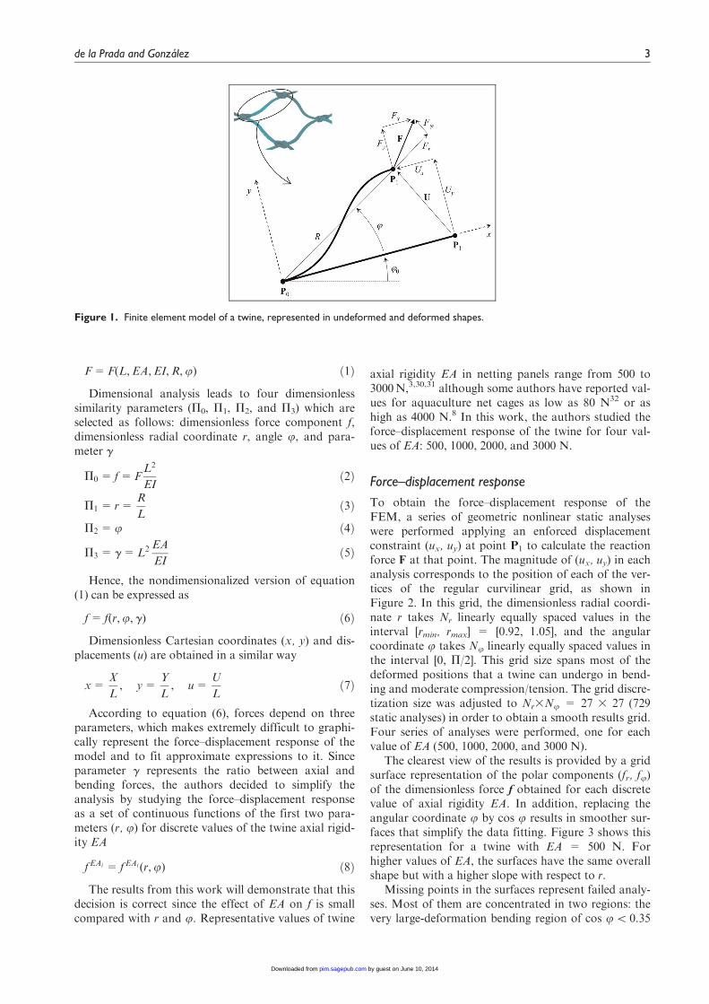
F=F(L,EA,EI,R,u) ð1Þ
Dimensional analysis leads to four dimensionlesssimilarity parameters (P0, P1, P2, and P3) which areselected as follows: dimensionless force component f,dimensionless radial coordinate r, angle u, and para-meter g
P0 = f=FL2
EIð2Þ
P1 = r=R
Lð3Þ
P2 =u ð4Þ
P3 = g =L2 EA
EIð5Þ
Hence, the nondimensionalized version of equation(1) can be expressed as
f= f(r,u, g) ð6Þ
Dimensionless Cartesian coordinates (x, y) and dis-placements (u) are obtained in a similar way
x=X
L, y=
Y
L, u=
U
Lð7Þ
According to equation (6), forces depend on threeparameters, which makes extremely difficult to graphi-cally represent the force–displacement response of themodel and to fit approximate expressions to it. Sinceparameter g represents the ratio between axial andbending forces, the authors decided to simplify theanalysis by studying the force–displacement responseas a set of continuous functions of the first two para-meters (r, u) for discrete values of the twine axial rigid-ity EA
fEAi = fEAi (r,u) ð8Þ
The results from this work will demonstrate that thisdecision is correct since the effect of EA on f is smallcompared with r and u. Representative values of twine
axial rigidity EA in netting panels range from 500 to3000N,3,30,31 although some authors have reported val-ues for aquaculture net cages as low as 80 N32 or ashigh as 4000 N.8 In this work, the authors studied theforce–displacement response of the twine for four val-ues of EA: 500, 1000, 2000, and 3000 N.
Force–displacement response
To obtain the force–displacement response of theFEM, a series of geometric nonlinear static analyseswere performed applying an enforced displacementconstraint (ux, uy) at point P1 to calculate the reactionforce F at that point. The magnitude of (ux, uy) in eachanalysis corresponds to the position of each of the ver-tices of the regular curvilinear grid, as shown inFigure 2. In this grid, the dimensionless radial coordi-nate r takes Nr linearly equally spaced values in theinterval [rmin, rmax] = [0.92, 1.05], and the angularcoordinate u takes Nu linearly equally spaced values inthe interval [0, P/2]. This grid size spans most of thedeformed positions that a twine can undergo in bend-ing and moderate compression/tension. The grid discre-tization size was adjusted to Nr3Nu = 27 3 27 (729static analyses) in order to obtain a smooth results grid.Four series of analyses were performed, one for eachvalue of EA (500, 1000, 2000, and 3000 N).
The clearest view of the results is provided by a gridsurface representation of the polar components (fr, fu)of the dimensionless force f obtained for each discretevalue of axial rigidity EA. In addition, replacing theangular coordinate u by cos u results in smoother sur-faces that simplify the data fitting. Figure 3 shows thisrepresentation for a twine with EA = 500 N. Forhigher values of EA, the surfaces have the same overallshape but with a higher slope with respect to r.
Missing points in the surfaces represent failed analy-ses. Most of them are concentrated in two regions: thevery large-deformation bending region of cos u \ 0.35
Figure 1. Finite element model of a twine, represented in undeformed and deformed shapes.
de la Prada and Gonzalez 3
by guest on June 10, 2014pim.sagepub.comDownloaded from
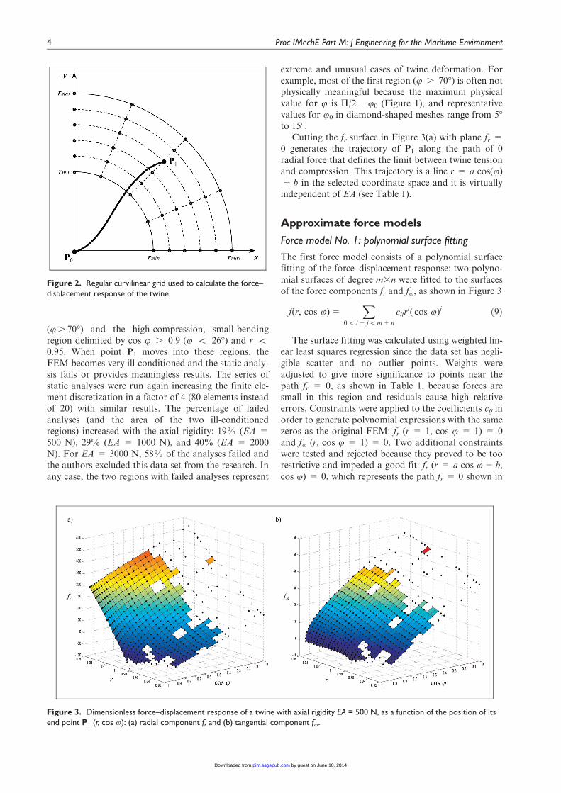
(u . 70�) and the high-compression, small-bendingregion delimited by cos u . 0.9 (u \ 26�) and r \0.95. When point P1 moves into these regions, theFEM becomes very ill-conditioned and the static analy-sis fails or provides meaningless results. The series ofstatic analyses were run again increasing the finite ele-ment discretization in a factor of 4 (80 elements insteadof 20) with similar results. The percentage of failedanalyses (and the area of the two ill-conditionedregions) increased with the axial rigidity: 19% (EA =500 N), 29% (EA = 1000 N), and 40% (EA = 2000N). For EA = 3000 N, 58% of the analyses failed andthe authors excluded this data set from the research. Inany case, the two regions with failed analyses represent
extreme and unusual cases of twine deformation. Forexample, most of the first region (u . 70�) is often notphysically meaningful because the maximum physicalvalue for u is P/2 2u0 (Figure 1), and representativevalues for u0 in diamond-shaped meshes range from 5�to 15�.
Cutting the fr surface in Figure 3(a) with plane fr =0 generates the trajectory of P1 along the path of 0radial force that defines the limit between twine tensionand compression. This trajectory is a line r = a cos(u)+ b in the selected coordinate space and it is virtuallyindependent of EA (see Table 1).
Approximate force models
Force model No. 1: polynomial surface fitting
The first force model consists of a polynomial surfacefitting of the force–displacement response: two polyno-mial surfaces of degree m3n were fitted to the surfacesof the force components fr and fu, as shown in Figure 3
f(r, cos u)=X
0\ i+ j\m+ n
cijri( cos u)j ð9Þ
The surface fitting was calculated using weighted lin-ear least squares regression since the data set has negli-gible scatter and no outlier points. Weights wereadjusted to give more significance to points near thepath fr = 0, as shown in Table 1, because forces aresmall in this region and residuals cause high relativeerrors. Constraints were applied to the coefficients cij inorder to generate polynomial expressions with the samezeros as the original FEM: fr (r = 1, cos u = 1) = 0and fu (r, cos u = 1) = 0. Two additional constraintswere tested and rejected because they proved to be toorestrictive and impeded a good fit: fr (r = a cos u+ b,cos u) = 0, which represents the path fr = 0 shown in
Figure 2. Regular curvilinear grid used to calculate the force–displacement response of the twine.
Figure 3. Dimensionless force–displacement response of a twine with axial rigidity EA = 500 N, as a function of the position of itsend point P1 (r, cos u): (a) radial component fr and (b) tangential component fu.
4 Proc IMechE Part M: J Engineering for the Maritime Environment
by guest on June 10, 2014pim.sagepub.comDownloaded from
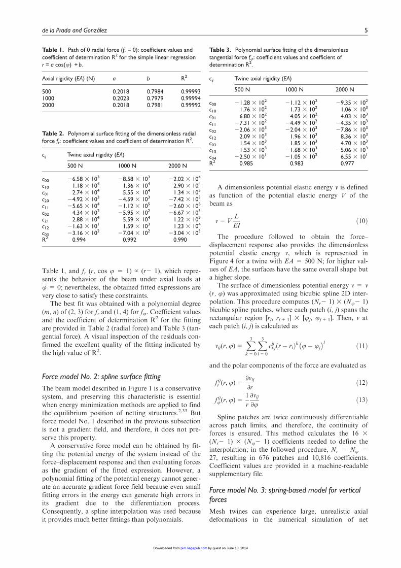
Table 1, and fr (r, cos u = 1) } (r2 1), which repre-sents the behavior of the beam under axial loads atu = 0; nevertheless, the obtained fitted expressions arevery close to satisfy these constraints.
The best fit was obtained with a polynomial degree(m, n) of (2, 3) for fr and (1, 4) for fu. Coefficient valuesand the coefficient of determination R2 for the fittingare provided in Table 2 (radial force) and Table 3 (tan-gential force). A visual inspection of the residuals con-firmed the excellent quality of the fitting indicated bythe high value of R2.
Force model No. 2: spline surface fitting
The beam model described in Figure 1 is a conservativesystem, and preserving this characteristic is essentialwhen energy minimization methods are applied to findthe equilibrium position of netting structures.2,33 Butforce model No. 1 described in the previous subsectionis not a gradient field, and therefore, it does not pre-serve this property.
A conservative force model can be obtained by fit-ting the potential energy of the system instead of theforce–displacement response and then evaluating forcesas the gradient of the fitted expression. However, apolynomial fitting of the potential energy cannot gener-ate an accurate gradient force field because even smallfitting errors in the energy can generate high errors inits gradient due to the differentiation process.Consequently, a spline interpolation was used becauseit provides much better fittings than polynomials.
A dimensionless potential elastic energy v is definedas function of the potential elastic energy V of thebeam as
v=VL
EIð10Þ
The procedure followed to obtain the force–displacement response also provides the dimensionlesspotential elastic energy v, which is represented inFigure 4 for a twine with EA = 500 N; for higher val-ues of EA, the surfaces have the same overall shape buta higher slope.
The surface of dimensionless potential energy v = v(r, u) was approximated using bicubic spline 2D inter-polation. This procedure computes (Nr2 1) 3 (Nu2 1)bicubic spline patches, where each patch (i, j) spans therectangular region [ri, ri+1] 3 [uj, uj+1]. Then, v ateach patch (i, j) is calculated as
vij(r,u)=X3k=0
X3l=0
cijkl r� rið Þk u� uj
� �l ð11Þ
and the polar components of the force are evaluated as
f ijr (r,u)=∂vij∂r
ð12Þ
f iju(r,u)=1
r
∂vij∂u
ð13Þ
Spline patches are twice continuously differentiableacross patch limits, and therefore, the continuity offorces is ensured. This method calculates the 16 3
(Nr2 1) 3 (Nu2 1) coefficients needed to define theinterpolation; in the followed procedure, Nr = Nu =27, resulting in 676 patches and 10,816 coefficients.Coefficient values are provided in a machine-readablesupplementary file.
Force model No. 3: spring-based model for verticalforces
Mesh twines can experience large, unrealistic axialdeformations in the numerical simulation of net
Table 1. Path of 0 radial force (fr = 0): coefficient values andcoefficient of determination R2 for the simple linear regressionr = a cos(u) + b.
Axial rigidity (EA) (N) a b R2
500 0.2018 0.7984 0.999931000 0.2023 0.7979 0.999942000 0.2018 0.7981 0.99992
Table 2. Polynomial surface fitting of the dimensionless radialforce fr: coefficient values and coefficient of determination R2.
cij Twine axial rigidity (EA)
500 N 1000 N 2000 N
c00 26.58 3 103 28.58 3 103 22.02 3 104
c10 1.18 3 104 1.36 3 104 2.90 3 104
c01 2.74 3 104 5.55 3 104 1.34 3 105
c20 24.92 3 103 24.59 3 103 27.42 3 103
c11 25.65 3 104 21.12 3 105 22.60 3 105
c02 4.34 3 102 25.95 3 102 26.67 3 103
c21 2.88 3 104 5.59 3 104 1.22 3 105
c12 21.63 3 101 1.59 3 103 1.23 3 104
c03 23.16 3 102 27.04 3 102 23.04 3 103
R2 0.994 0.992 0.990
Table 3. Polynomial surface fitting of the dimensionlesstangential force fu: coefficient values and coefficient ofdetermination R2.
cij Twine axial rigidity (EA)
500 N 1000 N 2000 N
c00 21.28 3 102 21.12 3 102 29.35 3 102
c10 1.76 3 102 1.73 3 102 1.06 3 103
c01 6.80 3 102 4.05 3 102 4.03 3 103
c11 27.31 3 102 24.49 3 102 24.35 3 103
c02 22.06 3 103 22.04 3 103 27.86 3 103
c12 2.09 3 103 1.96 3 103 8.36 3 103
c03 1.54 3 103 1.85 3 103 4.70 3 103
c13 21.53 3 103 21.68 3 103 25.06 3 103
c04 22.50 3 101 21.05 3 102 6.55 3 101
R2 0.985 0.983 0.977
de la Prada and Gonzalez 5
by guest on June 10, 2014pim.sagepub.comDownloaded from
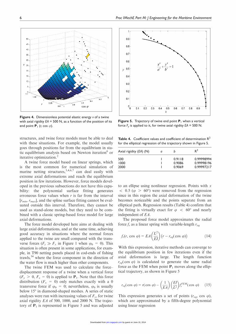
structures, and twine force models must be able to dealwith these situations. For example, the model usuallygoes through positions far from the equilibrium in sta-tic equilibrium analysis based on Newton iteration6 oriterative optimization.2
A twine force model based on linear springs, whichis the most common for numerical simulation ofmarine netting structures,3,4,6,7 can deal easily withextreme axial deformations and reach the equilibriumposition in few iterations. However, force models devel-oped in the previous subsections do not have this capa-bility: the polynomial surface fitting generateserroneous force values when r is far from the interval[rmin, rmax], and the spline surface fitting cannot be eval-uated outside this interval. Therefore, they cannot beused as stand-alone models, but they need to be com-bined with a classic spring-based force model for largeaxial deformations.
The force model developed here aims at dealing withlarge axial deformations, and at the same time, achievinggood accuracy in situations where the normal forcesapplied to the twine are small compared with the trans-verse forces (Fy � Fx in Figure 1 when u0 = 0). Thissituation is often present in some applications, for exam-ple, in T90 netting panels placed in cod-ends of fishingtrawls,34 where the force component in the direction ofthe water flow is much higher than other components.
The twine FEM was used to calculate the force–displacement response of a twine when a vertical force(Fy . 0, Fx = 0) is applied to P1. Note that this forcedistribution (Fx = 0) only matches exactly with a 0transverse force if u0 = 0; nevertheless, u0 is usuallybelow 15� in diamond-shaped meshes. A series of staticanalyses were run with increasing values of Fy, for twineaxial rigidity EA of 500, 1000, and 2000 N. The trajec-tory of P1 is represented in Figure 5 and was adjusted
to an ellipse using nonlinear regression. Points with x\ 0.5 (u . 60�) were removed from the regressionsince in this region the axial deformation of the twinebecomes noticeable and the points separate from anelliptical path. Regression results (Table 4) confirm thatthe fitting is virtually exact for u \ 60� and nearlyindependent of EA.
The proposed force model approximates the radialforce fr as a linear spring with variable-length req
fr(r, cos u)=EAL2
EI
� �r� req( cos u)� �
ð14Þ
With this expression, iterative methods can converge tothe equilibrium position in few iterations even if theaxial deformation is large. The length functionreq( cos u) is calculated to generate the same radialforce as the FEM when point P1 moves along the ellip-tical trajectory, as shown in Figure 5
req( cos u)= r( cos u)� 1
EA
� �EI
L2
� �f FEMr ( cos u) ð15Þ
This expression generates a set of points (req, cos u),which are approximated by a fifth-degree polynomialusing linear regression
Figure 4. Dimensionless potential elastic energy v of a twinewith axial rigidity EA = 500 N, as a function of the position of itsend point P1 (r, cos u).
Figure 5. Trajectory of twine end point P1 when a verticalforce Fy is applied to it, for twine axial rigidity EA = 500 N.
Table 4. Coefficient values and coefficient of determination R2
for the elliptical regression of the trajectory shown in Figure 5.
Axial rigidity (EA) (N) a b R2
500 1 0.9118 0.999989941000 1 0.9086 0.999981962000 1 0.9069 0.99997217
6 Proc IMechE Part M: J Engineering for the Maritime Environment
by guest on June 10, 2014pim.sagepub.comDownloaded from
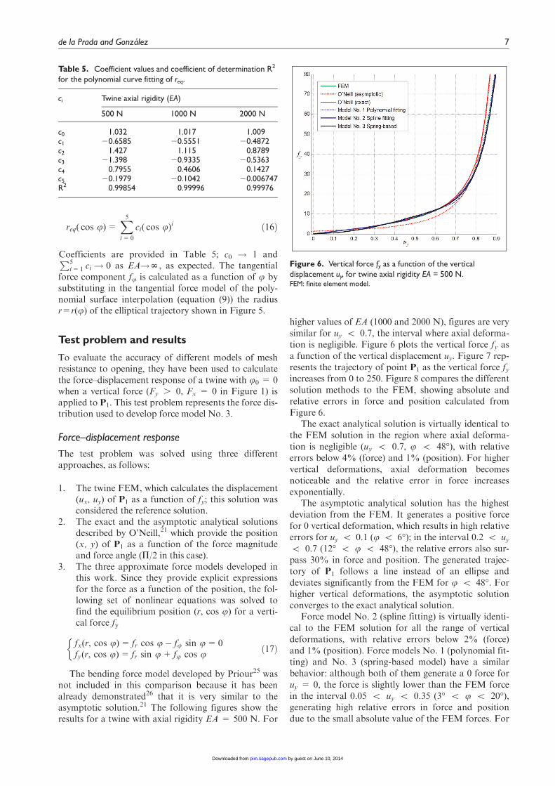
req( cos u)=X5i=0
ci( cos u)i ð16Þ
Coefficients are provided in Table 5; c0 ! 1 andP5i=1 ci ! 0 as EA!N, as expected. The tangential
force component fu is calculated as a function of u bysubstituting in the tangential force model of the poly-nomial surface interpolation (equation (9)) the radiusr=r(u) of the elliptical trajectory shown in Figure 5.
Test problem and results
To evaluate the accuracy of different models of meshresistance to opening, they have been used to calculatethe force–displacement response of a twine with u0 = 0when a vertical force (Fy . 0, Fx = 0 in Figure 1) isapplied to P1. This test problem represents the force dis-tribution used to develop force model No. 3.
Force–displacement response
The test problem was solved using three differentapproaches, as follows:
1. The twine FEM, which calculates the displacement(ux, uy) of P1 as a function of fy; this solution wasconsidered the reference solution.
2. The exact and the asymptotic analytical solutionsdescribed by O’Neill,21 which provide the position(x, y) of P1 as a function of the force magnitudeand force angle (P/2 in this case).
3. The three approximate force models developed inthis work. Since they provide explicit expressionsfor the force as a function of the position, the fol-lowing set of nonlinear equations was solved tofind the equilibrium position (r, cos u) for a verti-cal force fy
fx(r, cos u)= fr cos u� fu sin u=0fy(r, cos u)= fr sin u+ fu cos u
�ð17Þ
The bending force model developed by Priour25 wasnot included in this comparison because it has beenalready demonstrated26 that it is very similar to theasymptotic solution.21 The following figures show theresults for a twine with axial rigidity EA = 500 N. For
higher values of EA (1000 and 2000 N), figures are verysimilar for uy \ 0.7, the interval where axial deforma-tion is negligible. Figure 6 plots the vertical force fy asa function of the vertical displacement uy. Figure 7 rep-resents the trajectory of point P1 as the vertical force fyincreases from 0 to 250. Figure 8 compares the differentsolution methods to the FEM, showing absolute andrelative errors in force and position calculated fromFigure 6.
The exact analytical solution is virtually identical tothe FEM solution in the region where axial deforma-tion is negligible (uy \ 0.7, u \ 48�), with relativeerrors below 4% (force) and 1% (position). For highervertical deformations, axial deformation becomesnoticeable and the relative error in force increasesexponentially.
The asymptotic analytical solution has the highestdeviation from the FEM. It generates a positive forcefor 0 vertical deformation, which results in high relativeerrors for uy \ 0.1 (u \ 6�); in the interval 0.2 \ uy\ 0.7 (12� \ u \ 48�), the relative errors also sur-pass 30% in force and position. The generated trajec-tory of P1 follows a line instead of an ellipse anddeviates significantly from the FEM for u \ 48�. Forhigher vertical deformations, the asymptotic solutionconverges to the exact analytical solution.
Force model No. 2 (spline fitting) is virtually identi-cal to the FEM solution for all the range of verticaldeformations, with relative errors below 2% (force)and 1% (position). Force models No. 1 (polynomial fit-ting) and No. 3 (spring-based model) have a similarbehavior: although both of them generate a 0 force foruy = 0, the force is slightly lower than the FEM forcein the interval 0.05 \ uy \ 0.35 (3� \ u \ 20�),generating high relative errors in force and positiondue to the small absolute value of the FEM forces. For
Table 5. Coefficient values and coefficient of determination R2
for the polynomial curve fitting of req.
ci Twine axial rigidity (EA)
500 N 1000 N 2000 N
c0 1.032 1.017 1.009c1 20.6585 20.5551 20.4872c2 1.427 1.115 0.8789c3 21.398 20.9335 20.5363c4 0.7955 0.4606 0.1427c5 20.1979 20.1042 20.006747R2 0.99854 0.99996 0.99976
Figure 6. Vertical force fy as a function of the verticaldisplacement uy, for twine axial rigidity EA = 500 N.FEM: finite element model.
de la Prada and Gonzalez 7
by guest on June 10, 2014pim.sagepub.comDownloaded from
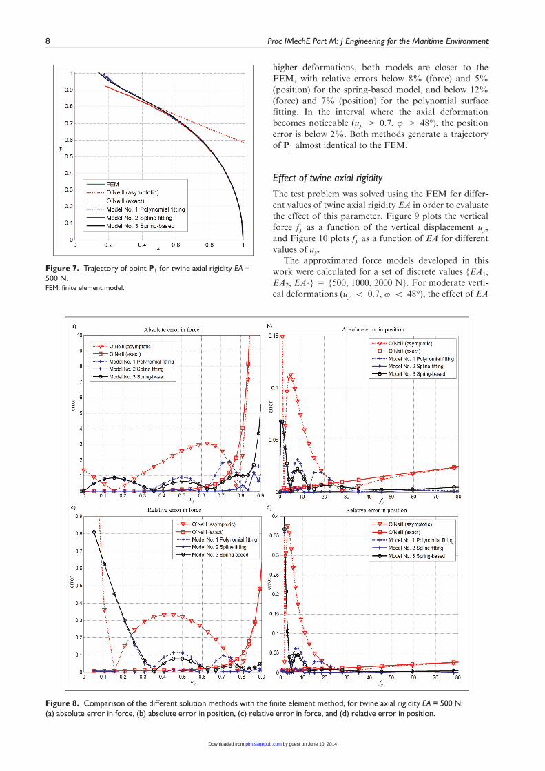
higher deformations, both models are closer to theFEM, with relative errors below 8% (force) and 5%(position) for the spring-based model, and below 12%(force) and 7% (position) for the polynomial surfacefitting. In the interval where the axial deformationbecomes noticeable (uy . 0.7, u . 48�), the positionerror is below 2%. Both methods generate a trajectoryof P1 almost identical to the FEM.
Effect of twine axial rigidity
The test problem was solved using the FEM for differ-ent values of twine axial rigidity EA in order to evaluatethe effect of this parameter. Figure 9 plots the verticalforce fy as a function of the vertical displacement uy,and Figure 10 plots fy as a function of EA for differentvalues of uy.
The approximated force models developed in thiswork were calculated for a set of discrete values {EA1,EA2, EA3} = {500, 1000, 2000 N}. For moderate verti-cal deformations (uy \ 0.7, u \ 48�), the effect of EA
Figure 7. Trajectory of point P1 for twine axial rigidity EA =500 N.FEM: finite element model.
Figure 8. Comparison of the different solution methods with the finite element method, for twine axial rigidity EA = 500 N:(a) absolute error in force, (b) absolute error in position, (c) relative error in force, and (d) relative error in position.
8 Proc IMechE Part M: J Engineering for the Maritime Environment
by guest on June 10, 2014pim.sagepub.comDownloaded from
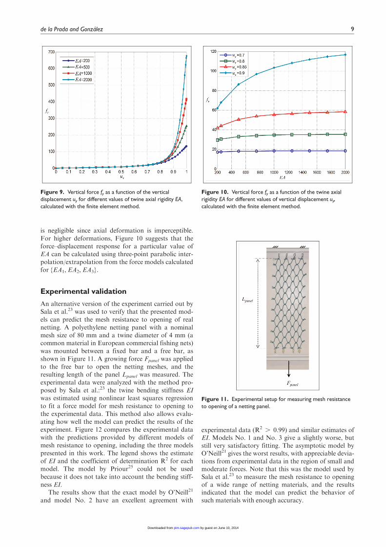
is negligible since axial deformation is imperceptible.For higher deformations, Figure 10 suggests that theforce–displacement response for a particular value ofEA can be calculated using three-point parabolic inter-polation/extrapolation from the force models calculatedfor {EA1, EA2, EA3}.
Experimental validation
An alternative version of the experiment carried out bySala et al.23 was used to verify that the presented mod-els can predict the mesh resistance to opening of realnetting. A polyethylene netting panel with a nominalmesh size of 80 mm and a twine diameter of 4 mm (acommon material in European commercial fishing nets)was mounted between a fixed bar and a free bar, asshown in Figure 11. A growing force Fpanel was appliedto the free bar to open the netting meshes, and theresulting length of the panel Lpanel was measured. Theexperimental data were analyzed with the method pro-posed by Sala et al.:23 the twine bending stiffness EIwas estimated using nonlinear least squares regressionto fit a force model for mesh resistance to opening tothe experimental data. This method also allows evalu-ating how well the model can predict the results of theexperiment. Figure 12 compares the experimental datawith the predictions provided by different models ofmesh resistance to opening, including the three modelspresented in this work. The legend shows the estimateof EI and the coefficient of determination R2 for eachmodel. The model by Priour25 could not be usedbecause it does not take into account the bending stiff-ness EI.
The results show that the exact model by O’Neill21
and model No. 2 have an excellent agreement with
experimental data (R2 . 0.99) and similar estimates ofEI. Models No. 1 and No. 3 give a slightly worse, butstill very satisfactory fitting. The asymptotic model byO’Neill21 gives the worst results, with appreciable devia-tions from experimental data in the region of small andmoderate forces. Note that this was the model used bySala et al.23 to measure the mesh resistance to openingof a wide range of netting materials, and the resultsindicated that the model can predict the behavior ofsuch materials with enough accuracy.
Figure 9. Vertical force fy as a function of the verticaldisplacement uy for different values of twine axial rigidity EA,calculated with the finite element method.
Figure 10. Vertical force fy as a function of the twine axialrigidity EA for different values of vertical displacement uy,calculated with the finite element method.
Figure 11. Experimental setup for measuring mesh resistanceto opening of a netting panel.
de la Prada and Gonzalez 9
by guest on June 10, 2014pim.sagepub.comDownloaded from
Discussion
The FEM used in this work assumes that the twinebehavior follows the Timoshenko beam theory, andthat the slope angle u0 between the twine and the knotsat the insertion points remains fixed. These assump-tions are unlikely to hold exactly for all kinds of nettingmaterials due to the complex structure of the constitu-ent fibers of fishing netting, and more experimentalwork will be needed to evaluate their validity. In addi-tion, the beam theory is often not valid to represent thebehavior of twines in moderate or high compression. Inspite of this the FEM makes less assumptions abouttwine behavior that previously existing models,21 sinceit takes into account axial deformations and geometricnonlinearities caused by large rotations.
The results from the test problem support the selectsize [rmin, rmax] = [0.92, 1.05] for the regular curvilineargrid used to calculate the force–displacement responseof the twine FEM (Figure 2): the dimensionless radialcoordinate r was bounded to this interval for u \ 80�(Figure 7), and higher values of u are often impractic-able due to physical limitations (umax = P/2 2u0).For situations different from the test problem, that is,Fx . 0 and Fy . 0, then umax = tan21(Fy/Fx) and thebehavior in Figures 7 and 9 indicates that r will notexceed rmax = 1.05 for the usual values of EA, unlessextremely high forces are applied.
The results also support the decision of studying theforce–displacement response of the beam model as a setof continuous functions of (r, u) for discrete values of
the twine axial rigidity EA. This decision was based onthe assumption that the effect of EA on the dimension-less forces is small compared with r and u. Accordingto Figures 9 and 10, the effect of EA is insignificant formoderate vertical deformations of the mesh (uy \ 0.7,u \ 48�). The effect of EA is only noticeable for verylarge vertical deformations (uy . 0.8, u . 60�), butsuch deformations hardly happen in real marine netstructures because the applied forces are not so high. Inany case, the presented approach is able to take intoaccount the small effect of EA using the aforemen-tioned three-point parabolic interpolation from theforce models calculated for {EA1, EA2, EA3}.
The behavior of the asymptotic analytical solutionagrees with the results reported by O’Neill,21 whichshows that it is very accurate in comparison to the exactanalytical solution for f . 25. On the other hand, thissolution has significant errors in force and position forsmaller values of the dimensionless force f (equivalentto u \ 50� in the test problem), especially in the trajec-tory of the twine end point, and this fact could partiallyexplain the lack of fit with experimental results reportedby Sala et al.23
Another interesting matter is related to the fact thatmost numerical formulations for flexible net structuresmodel the axial behavior of the twine as a linear spring,and therefore assume that its natural length remainsconstant during mesh opening.3,4,6,7 Table 1 revealsthat this assumption is not correct since the length cor-responding to a 0 axial force decreases as the bendingangle increases. The same conclusion could be achievedusing the exact analytical solution,21 which generates asimilar shape for a bending twine (Figure 7). As aresult, the mesh shape and dimensions calculated bysuch formulations will differ from the actual values,and this fact has an impact on the accuracy of selectiv-ity of fishing gears calculated with those methods.Conversely, the three developed force models take intoaccount the coupling between axial and bending defor-mations, and therefore, it is expected that they can gen-erate more precise mesh shapes.
Regarding computational efficiency of the evalua-tion of forces as a function of twine deformation, thethree approximate force models are extremely efficientdue to their explicit and simple expressions, even forforce model No. 2 (spline surface fitting). Conversely,the computational cost of the asymptotic analyticalsolution is notably higher, and the exact analytical solu-tion proved to be extremely inefficient.
The numerical and experimental validations carriedout in this work are based on static analysis. Hence, thiswork does not demonstrate that the presented modelsare efficient and accurate for dynamic analysis. But theresults show that they are better (i.e. significantly fasterwith similar or even better accuracy) than existing mod-els developed by Priour25 and O’Neill21 when applied tostatic analysis. Therefore, it is reasonable to supposethat they will also perform better than such existing
Figure 12. Length of the netting panel in normal meshdirection Lpanel as a function of the applied force Fpanel. Fittingsobtained with different models of mesh resistance to openingare shown: the exact and asymptotic models by O’Neill21 andthe three models presented in this work. Model No. 1 refers tothe polynomial fitting of the force, Model No. 2 refers to thespline fitting of the potential energy, and Model No. 3 refers tothe spring-based model. The legend also provides the estimatesfor twine bending stiffness EI and the coefficient ofdetermination R2 for each model.
10 Proc IMechE Part M: J Engineering for the Maritime Environment
by guest on June 10, 2014pim.sagepub.comDownloaded from
models when applied to dynamic analysis. Furtherresearch must be carried out to verify this hypothesis.
Finally, Table 6 summarizes the differences betweenthe three presented force models and previous modelsfor mesh resistance to opening. The comparison showsthat the models developed in this work have strongadvantages over previous models. The comparison alsohelps to choose which one of the three presented forcemodels is best suited for a particular application.
Conclusion
A FEM of a twine has been used to develop threedimensionless approximate force models of mesh resis-tance to opening, which express elastic forces in a twineas explicit functions of twine deformation. Each forcemodel has different features, and researchers canchoose which one better fits the requirements of a par-ticular application:
1. A polynomial fitting of the force components, withgood accuracy and extremely easy to implement.
2. A spline fitting of the potential energy, which gen-erates a highly accurate, conservative force fieldsuitable to energy optimization methods, at thecost of a slightly more complex implementation.
3. A spring-based model able to deal with large axialdeformations, designed for situations where thenormal forces applied to the twine are small com-pared with the transverse forces.
The developed force models have good accuracy andhigh computational efficiency. They will allow introdu-cing accurate simulation of mesh opening resistance inexisting numerical formulations for marine nettingstructures without a high impact in their computationalperformance. In the future, the authors will apply thesemodels to the static and dynamic analysis of such struc-tures under hydrodynamic loads. Furthermore, theymay also be useful to analyze data from experimentalwork to measure mesh resistance to opening, with the
intention of achieving a better goodness of fit with pre-vious force models. However, several questions remainopen and require further research, such as the behaviorof force models No. 1 and No. 2 under large axialdeformations.
Declaration of conflicting interests
The authors declare that there is no conflict of interest.
Funding
This research received no specific grant from any fund-ing agency in the public, commercial, or not-for-profitsectors.
References
1. Ito S, Kinoshita T and Bao W. Hydrodynamic beha-
viours of elastic net sheets in waves. Proc IMechE, Part
M: J Engineering for the Maritime Environment 2012;
226(2): 156–169.2. Le Dret H, Lewandowski R, Priour D, et al. Numerical
simulation of a cod end net part 1: equilibrium in a uni-
form flow. J Elasticity 2004; 76(2): 139–162.3. Lee C-W, Lee J-H, Cha B-J, et al. Physical modeling for
underwater flexible systems dynamic simulation. Ocean
Eng 2005; 32(3–4): 331–347.4. Li Y-C, Zhao Y-P, Gui F-K, et al. Numerical simulation
of the hydrodynamic behaviour of submerged plane nets
in current. Ocean Eng 2006; 33(17–18): 2352–2368.
5. O’Neill FG. Axisymmetric trawl cod-ends made from
netting of a generalized mesh shape. IMA J Appl Math
1999; 62(3): 245–262.6. Priour D. Calculation of net shapes by the finite element
method with triangular elements. Commun Numer Meth
Eng 1999; 15(10): 755–763.7. Takagi T, Shimizu T, Suzuki K, et al. Validity and lay-
out of ‘‘NaLA’’: a net configuration and loading analysis
system. Fish Res 2004; 66(2–3): 235–243.8. Tsukrov I, Eroshkin O, Fredriksson D, et al. Finite ele-
ment modeling of net panels using a consistent net ele-
ment. Ocean Eng 2003; 30(2): 251–270.9. Priour D, Herrmann B and O’Neill FG. Modelling axi-
symmetric cod-ends made of different mesh types. Proc
Table 6. Comparison of the presented force models (De la Prada and Gonzalez) with previous models of mesh resistance toopening by Priour25 and O’Neill.21
Features Priour25 O’Neill21 De la Prada and Gonzalez
Exact Asymptotic No. 1 No. 2 No. 3
Takes into account twine bending stiffness (EI) – � � � � �Takes into account twine axial stiffness (EA) – – – � � �Force as explicit function of position (i.e. fast evaluation of forces) � – – � � �Highly accurate – � – � � �Very easy to implement in existing formulations � – – � – �Conservative force field � – – – � –Compatible with large twine axial deformations – – – – – �Compatible with high transversal forces � � � � � –
Model No. 1 refers to the polynomial fitting of the force, Model No. 2 refers to the spline fitting of the potential energy, and Model No. 3 refers to
the spring-based model.
de la Prada and Gonzalez 11
by guest on June 10, 2014pim.sagepub.comDownloaded from
IMechE, Part M: J Engineering for the Maritime Environ-
ment 2009; 223(1): 137–144.10. DeCew J, Tsukrov I, Risso A, et al. Modeling of dynamic
behavior of a single-point moored submersible fish cage
under currents. Aquac Eng 2010; 43(2): 38–45.11. Herrmann B, Priour D and Krag LA. Theoretical study
of the effect of round straps on the selectivity in a dia-
mond mesh cod-end. Fish Res 2006; 80(2–3): 148–157.12. Khaled R, Priour D and Billard J-Y. Numerical optimi-
zation of trawl energy efficiency taking into account fish
distribution. Ocean Eng 2012; 54: 34–45.13. Lee J, Lee C-W, Choe M-Y, et al. Applying fishing-gear
simulation software to better estimate fished space as fish-
ing effort. Fish Aquat Sci 2011; 14(2): 138–147.14. Shimizu T, Takagi T, Korte H, et al. Application of
NaLA, a fishing net configuration and loading analysis
system, to bottom gill nets. Fish Sci 2007; 73(3): 489–499.15. Xu T-J, Dong G-H, Zhao Y-P, et al. Analysis of hydro-
dynamic behaviors of gravity net cage in irregular waves.
Ocean Eng 2011; 38(13): 1545–1554.16. Herrmann B. Effect of catch size and shape on the selec-
tivity of diamond mesh cod-ends: I. Model development.
Fish Res 2005; 71(1): 1–13.17. Herrmann B and O’Neill FG. Theoretical study of the
influence of twine thickness on haddock selectivity in dia-
mond mesh cod-ends. Fish Res 2006; 80(2–3): 221–229.18. Sala A, Lucchetti A and Buglioni G. The influence of
twine thickness on the size selectivity of polyamide
codends in a Mediterranean bottom trawl. Fish Res 2007;
83(2–3): 192–203.19. O’Neill FG. The influence of bending stiffness on the
deformation of axisymmetric networks. In: Proceedings
of the international conference on offshore mechanics and
arctic engineering—OMAE, Vancouver, BC, Canada, 20–
25 June 2004, pp.749–754. New York: ASME.20. O’Neill FG and Xu L. Twine flexural rigidity and mesh
resistance to opening. In: ICES CM (1994/B:31), Interna-
tional Council for the Exploration of the Sea (ICES),
Copenhagen, Denmark: 25–26 April 1994.21. O’Neill FG. Bending of twines and fibres under tension.
J Textil Inst 2002; 93(1): 1–8.
22. O’Neill FG. A theoretical study of the factors whichinfluence the measurement of fishing netting mesh size.Ocean Eng 2003; 30(16): 2053–2063.
23. Sala A, O’Neill FG, Buglioni G, et al. Experimentalmethod for quantifying resistance to the opening of net-ting panels. ICES J Marine Sci 2007; 64(8): 1573–1578.
24. Behbahani-Nejad M and Perkins NC. Hydrodynamicand geometric stiffening effects on the out-of-plane wavesof submerged cables. Nonlinear Dynam 1997; 13(3):243–257.
25. Priour D. Introduction of mesh resistance to opening in atriangular element for calculation of nets by the finite ele-ment method. Commun Numer Meth Eng 2001; 17(4):229–237.
26. O’Neill FG and Priour D. Comparison and validation oftwo models of netting deformation. J Appl Mech: T
ASME 2009; 76(5): 1–7.
27. Peirce FT. The ‘‘Handle’’ of cloth as a measurable quan-tity. J Textil Inst Trans 1930; 21(9): T377–T416.
28. Abbott GM. Yarn-bending and the weighted-ring stiff-ness test. J Textil Inst 1983; 74(5): 281–286.
29. Du Z-Q, Zhou T, Yan N, et al. Measurement and char-acterization of bending stiffness for fabrics. Fiber Polym2011; 12(1): 104–110.
30. Lee C-W, Kim Y-B, Lee G-H, et al. Dynamic simulationof a fish cage system subjected to currents and waves.Ocean Eng 2008; 35(14–15): 1521–1532.
31. Sala A, Lucchetti A and Buglioni G. The change in phys-ical properties of some nylon (PA) netting samples beforeand after use. Fish Res 2004; 69(2): 181–188.
32. Moe H, Olsen A, Hopperstad OS, et al. Tensile properties
for netting materials used in aquaculture net cages. AquacEng 2007; 37(3): 252–265.
33. De la Prada A and Gonzalez M. Assessing the suitabilityof gradient-based energy minimization methods to calcu-late the equilibrium shape of netting structures. Comput
Struct 2014; 135: 128–140.34. Herrmann B, Priour D and Krag LA. Simulation-based
study of the combined effect on cod-end size selection ofturning meshes by 90� and reducing the number ofmeshes in the circumference for round fish. Fish Res
2007; 84(2): 222–232.
12 Proc IMechE Part M: J Engineering for the Maritime Environment
by guest on June 10, 2014pim.sagepub.comDownloaded from

Efficient and accurate methods for computational simulation of netting structures with mesh resistance to opening Ph. D. Thesis
Amelia de la Prada
Article No. 2
Quantifying mesh resistance to opening of
netting panels: experimental method, regression
models and parameter estimation strategies
Amelia de la Prada, Manuel González
Submitted to the ICES Journal of Marine Science on 10th April 2014
Revised version submitted on 30th May 2014
Revised version submitted on 17th June 2014
Accepted for publication on 23rd June 2014

1
Quantifying mesh resistance to opening of
netting panels: experimental method, regression
models and parameter estimation strategies
Amelia de la Prada, Manuel González*
Laboratorio de Ingeniería Mecánica ─ Universidade da Coruña
Escuela Politécnica Superior, Mendizábal s/n, 15403 Ferrol, Spain
E-mail address: [email protected], [email protected]
* Corresponding author. E-mail address: [email protected]
Tel.: (+34) 981337400 fax: (+34) 981337410
2
Abstract
The increased mesh resistance to opening of netting panels manufactured with thick and
stiff twines has a notable impact in the structural response and selective performance of
the fishing gears. The only available method to quantify the mesh resistance to opening
of netting panels was described in (Sala et al., 2007b). We present an alternative method
with a similar methodology: we attempt to estimate the mechanical and geometrical
properties of a netting material that best fits the experimental measurements of a netting
panel. We introduce three major contributions: (i) a considerably simpler uniaxial
experimental setup, which stretches a netting sample in the normal direction of the
meshes while leaving free its deformation in the transverse direction; (ii) more accurate
theoretical models for mesh resistance to opening; (iii) new strategies to estimate the
parameters of the models. We present the results of the analysis of polyethylene (PE),
compacted polyethylene (CPE), single-twine and double-twine netting. Some of the
assessed combinations of estimation strategies and theoretical models have an excellent
goodness of fit with experimental data. The method proved to be a simple yet accurate
way to quantify the mesh resistance to opening of netting panels.
Keywords: bending stiffness; flexural rigidity; mesh resistance to opening; twine;
regression
3
Introduction
In recent years, there is a tendency in some sectors of the fishing industry towards the
use of thicker and stiffer twines in the manufacture of netting materials for the codend
of trawls. The increased mesh resistance to opening of such materials has a notable
impact in the structural response and performance of the fishing gears. For example, an
increased mesh resistance to opening hinders mesh opening in the cod-end (O’Neill,
2004), which affects the escapement of small fish. Theoretical and experimental studies
demonstrate that mesh resistance to opening plays as major role in the reduction of
selective performance of trawls (Herrmann and O’Neill, 2006; Herrmann et al., 2013;
Lowry and Robertson, 1996; Sala et al., 2007a). Theoretical models for mesh resistance
to opening are generally based on the beam theory of solid mechanics. In diamond mesh
panels, the predominant netting in towed fishing gears, the resistance to opening is
mainly characterized by the bending stiffness of the netting twine. An increased twine
bending stiffness also changes the overall shape of the fishing gear during fishing
operations (O’Neill, 2004; Priour, 2001). Therefore, methods to quantify the mesh
resistance to opening and to incorporate this property in theoretical models of netting
materials are necessary to accurately predict the selective performance of fishing gears
by simulation. Despite this, research about this topic is still scarce (Priour and Cognard,
2011).
The only available method to quantify mesh resistance to opening of netting panels is
described in (Sala et al., 2007b). The method uses a specially designed instrument that
applies normal and transversal displacements to a netting sample and measures the
generated reaction forces. Then, twine bending stiffness and geometric parameters of
the netting are estimated through nonlinear regression analysis of the obtained
experimental data. The asymptotic solution for a bending twine proposed in (O’Neill,

4
2002) is used as model in the regression analysis. Although the method proved to be
robust and useful to estimate mesh resistance to opening, the authors reported several
problems: inconsistencies between normal and transversal forces and displacements,
occasional unrealistic estimates of geometrical parameter values and systematic lack of
fit of the model to the experimental data. Another concern is that the authors carried out
the regression analysis using the force as independent variable and the displacement as
dependent variable, despite the force was an effect caused by an applied displacement in
the experimental setup. The complexity of the experimental setup required by this
method is another important drawback.
A method to estimate twine bending stiffness was proposed by (Priour and Cognard,
2011). The method measures the out-of-plane bending deformation of a netting sample
and then adjusts a theoretical model of a cantilever beam to the experimental data, in
order to estimate the twine bending stiffness EI. The method is very simple, but it has
some drawbacks. It does not take into account the knot size, which can have an
important effect on the shape of the codends (PREMECS: Development of predictive
model of cod-end selectivity, 2000). In addition, and it cannot estimate the slope angle
between twines and knots at the insertion points.
The goal of this article is to describe a simple but accurate experimental method to
quantify the mesh resistance to opening of netting panels. We follow a methodology
similar to (Sala et al., 2007b), that is, we attempt to estimate the mechanical and
geometrical properties of a netting material that best fit the experimental measurements
of a netting panel. This research introduces three original contributions:
(i) The biaxial experimental setup used in (Sala et al., 2007b) requires a very complex
measurement instrument which is not commercially available. In contrast, this work

5
proposes a new uniaxial experimental setup that notably simplifies the required
measurement instrument.
(ii) The regression model used in (Sala et al., 2007b) is the asymptotic model for a
bending twine described in (O’Neill, 2002). This model is an approximate solution. This
work uses more accurate models to describe mesh resistance to opening: the exact
model described in (O’Neill, 2002) and two recently developed models based on finite
element analysis (de la Prada and González, 2014a).
(iii) The parameter estimation strategy used in (Sala et al., 2007b) fixed one of the
geometrical properties of the netting (the slope angle between the twine and the knots)
and leaved the remaining parameters unconstrained. As results, the estimates were
sometimes out of physical limits. This work assesses other estimation strategies that
avoid that problem.
Material and Methods
Theoretical models for mesh resistance to opening
Priour proposed a theoretical model for mesh resistance to opening based on the
assumption that the couple created by mesh twines on the knot varies linearly with the
angle between twines (Priour, 2001). Although this model can be easily introduced in
numerical formulations for netting structures, it does not involve parameters with
specific physical interpretation, and therefore it is not suited to identify the mechanical
properties of the netting (e.g. twine bending stiffness) from experimental data.
O'Neill proposed a physically-oriented approach to the problem (O’Neill, 2002) by
modelling the twine as a bi-dimensional double-clamped beam (Figure 1) and
describing the equations governing its bending assuming that: (i) the slope angle
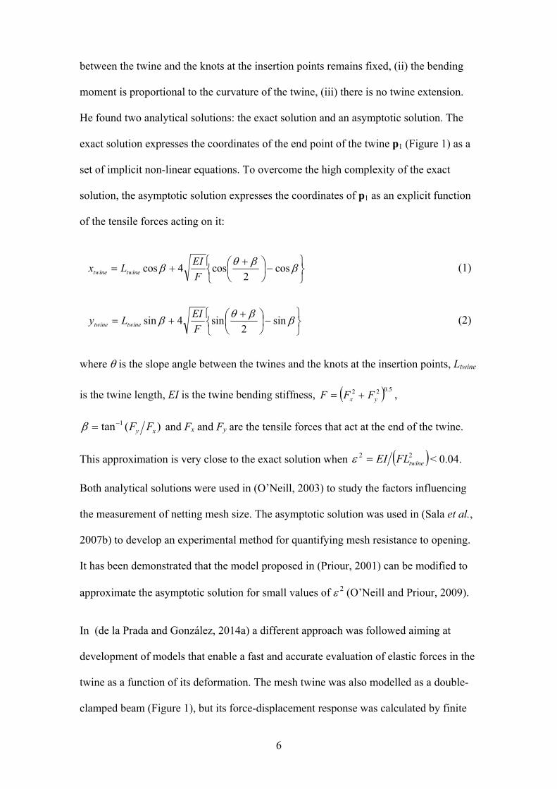
6
between the twine and the knots at the insertion points remains fixed, (ii) the bending
moment is proportional to the curvature of the twine, (iii) there is no twine extension.
He found two analytical solutions: the exact solution and an asymptotic solution. The
exact solution expresses the coordinates of the end point of the twine p1 (Figure 1) as a
set of implicit non-linear equations. To overcome the high complexity of the exact
solution, the asymptotic solution expresses the coordinates of p1 as an explicit function
of the tensile forces acting on it:
cos2
cos4cosF
EILx twinetwine (1)
sin2
sin4sinF
EILy twinetwine (2)
where is the slope angle between the twines and the knots at the insertion points, Ltwine
is the twine length, EI is the twine bending stiffness, 5.022yx FFF ,
)(tan 1xy FF and Fx and Fy are the tensile forces that act at the end of the twine.
This approximation is very close to the exact solution when 22twineFLEI < 0.04.
Both analytical solutions were used in (O’Neill, 2003) to study the factors influencing
the measurement of netting mesh size. The asymptotic solution was used in (Sala et al.,
2007b) to develop an experimental method for quantifying mesh resistance to opening.
It has been demonstrated that the model proposed in (Priour, 2001) can be modified to
approximate the asymptotic solution for small values of 2 (O’Neill and Priour, 2009).
In (de la Prada and González, 2014a) a different approach was followed aiming at
development of models that enable a fast and accurate evaluation of elastic forces in the
twine as a function of its deformation. The mesh twine was also modelled as a double-
clamped beam (Figure 1), but its force-displacement response was calculated by finite
7
element analysis (Zienkiewicz, 2000). Then, fitting techniques were used to develop
two dimensionless models. The first model, named the polynomial model, fits a
polynomial of the radial and tangential force components Fr and F that act at the end of
the twine. This results in a polynomial degree (m,n) of (2,3) for Fr and (1,4) for F:
j
nmji
iij
twiner rc
L
EIrF cos ,
02
(3)
j
nmji
iij
twine
rcL
EIrF cos ,
02
(4)
where twinetwinetwine Lyxr5.022 , )(tan 1
twinetwine xy and = .
The second model, called the spline model, calculates Fr and F as the gradient of the
potential elastic energy V of the twine. V was interpolated with (Nr 1)×( N 1) bicubic
spline patches, where each patch (i, j) spans the rectangular region [ri, ri+1]×[j , j+1]
and expresses V as:
ljk
ik l
ijkl
twineij rrc
L
EIrV
3
0
3
0
, (5)
A comprehensive description of the polynomial and spline models is provided in (de la
Prada and González, 2014a), with comparisons to the abovementioned exact and
asymptotic models described in (O’Neill, 2002). The spline model is very accurate and
it is well suited for simulation methods based on energy minimization (de la Prada and
González, 2014b). The polynomial model has a simpler mathematical form at the cost
of a slightly lower accuracy (5% 10% of deviation), as reported in (de la Prada and
González, 2014a).
8
Experimental setup
The experimental setup is portrayed in Figure 2. A rectangular netting sample is
attached between an upper fixed bar and a bottom free bar, with the normal direction of
the meshes aligned to the vertical axis of the figure (i.e. perpendicular to the bars). The
free bar can move in the normal direction of the netting while keeping its orientation
parallel to the fixed bar. The attachment system between the netting sample and the bars
allows the netting knots to freely move in the transverse direction of the netting when
the sample is stretched. In this way, the force applied to meshes and twines in the
transverse direction of the netting is zero. The panel has mn and mt netting meshes in
normal and transverse direction respectively. During the experiment, the sample is
stretched in the normal direction of the netting to open the meshes.
The sample is stretched by applying a force Fpanel to the free bar. The normal length of
the panel Lpanel, defined as the distance between centres of the upper and bottom knots,
is calculated as Lpanel = D0 (DR+DL)/2 D1 D2, where distances D0, D1 and D2 are
measured at the beginning of the experiment and distances DR and DL are measured for
each value of Fpanel (both distances should be equal in theory, but in practice slight
differences can appear due to misalignment of the free bar). Fpanel is generated by
applying calibrated weights to the free bar. The weight of the free bar (0.68 N) and
mounting hooks (0.04 N each) is also included in Fpanel. Distances D1 and D2 are
measured with a Vernier calliper, while distances D0, DR and DL are measured with
digital laser rangefinders with an accuracy of 0.5 mm. Other measuring procedures are
also compatible with the experimental setup described in Figure 2: for example, Lpanel
could be prescribed and the required Fpanel could be measured.

9
The objective of this work is not to quantify the mesh resistance to opening for a wide
range of netting materials, but rather to investigate different combinations of regression
models and parameter estimation strategies for the proposed uniaxial experimental
setup. Hence, a number of new and unused netting samples were tested. All of them are
used in commercial North Sea trawls. Their main characteristics are given in Table 1:
materials are sorted according to the perceived mesh resistance to opening from manual
manipulation of the netting, from low (PE 802.5) to high (CPE2 804) stiffness.
The following steps were performed for each netting sample:
i. The netting is attached to the bars and distances D1 and D2 are measured. At this
moment Fpanel is equal to the weight of the bottom free bar and hooks (0.7 N).
ii. Fpanel is increased. Load increments start with 0.5 N and increase up to a
maximum value of 9.8 N as Lpanel increases.
iii. Distances DR and DL are measured at every minute to monitor netting twine
relaxation (Sala et al., 2007b); when they get stabilized, the final values are
recorded.
iv. Steps (ii) and (iii) are repeated until Lpanel reaches 80% of mnLmesh, where Lmesh
is the nominal mesh size. Above this value, the main characteristic contributing
to mesh resistance to opening is twine axial stiffness EA rather than twine
bending stiffness EI (de la Prada and González, 2014a).
Netting materials used in fishing gears may experience high tensile forces able to
generate permanent plastic deformations in twines and knots. To simulate such situation
in the experimental setup, the maximum value of Fpanel reached in step (iv) is applied for
one hour to the netting. Then steps (ii) and (iii) are repeated with decreasing values of

10
Fpanel in step (ii). In this way two sets of data are obtained: a loading cycle and an
unloading cycle.
Data analysis
To analyse the experimental data it is necessary to make the same assumptions as in
(Sala et al., 2007b), which define the idealized panel represented in Figure 3: (i) the
netting is homogeneous, so all the meshes experience the same deformation, (ii) knots
can be represented as rectangles of size a b, and (iii) twines emerge from knots at the
corners of the rectangles. Note that the knot size a b is smaller than the measured
outer knot size aext bext given in Table 1. The mechanical and geometrical parameters
of this idealized netting panel are estimated by fitting theoretical models for mesh
resistance to opening to experimental data. The observed variable in the experiment is
the distance between twine knots in the normal direction of the netting
npanelknots mLy 2 (6)
and the explanatory variable is the vertical force applied to the twines
tpanely mFF 2 (7)
The predicted values for the distance between knots can be expressed as
,,ˆ twinetwineknots LEIyby (8)
where ytwine can be calculated with any theoretical model for mesh resistance to opening.
Therefore, four parameters can be estimated: EI, Ltwine, b and . Notice that the knot
dimension a cannot be estimated with the proposed experimental setup because the
transversal length of the panel is not measured. Preliminary analysis show that there are
not outlier points in the experimental data. For simplicity, the observed and the
11
explanatory variables are assumed to be distributed with constant variance. Therefore,
nonlinear least squares regression is used (Seber, 1989).
With respect to the regression model ,, twinetwine LEIy in Eq. (8), the four models for
mesh resistance to opening described in Section 2 were assessed: the exact model, the
asymptotic model, the polynomial model and spline model. The use of the asymptotic
model is straightforward, since it provides twiney as an explicit function of the
explanatory variable Fy. The other models need to be numerically solved for every
evaluation in the regression analysis.
A remark must be made regarding the use of the asymptotic model in this experimental
setup, where Fx = 0 )(tan 1xy FF = /2 in Eq. 1 and 2. The asymptotic
approximation is very close to the exact solution when 2 < 0.04 (O’Neill, 2002), but 2
usually ranges from 0.4 and 0.1 in most part of the loading and unloading cycles of our
experiments. This is explained in Figure 4, which shows the dimensionless vertical
displacement of the twine calculated with Eq. 2 for = /2, as a function of the
parameter 2 = )( 2twineFLEI and the slope angle . Since Fx = 0, the mesh can be opened
in normal direction with a relatively small force. Hence, the condition 2 < 0.04 can only
be achieved provided that is small and the mesh is nearly completely opened
(ytwine/Ltwine ≥ 0.75). The only way to achieve 2 < 0.04 without completely opening the
mesh is to apply a transversal force Fx > 0 to reduce as in the experimental setup used
in (Sala et al., 2007b). Nevertheless, (de la Prada and González, 2014a) shows that the
vertical position of the twine twiney predicted by the asymptotic model is close to the
exact model even if = /2 (relative error below 10% in most of the range of
displacement), because most of the error in this model is in the horizontal position xtwine.
12
As a result, the asymptotic solution can still be used as model in this experimental setup,
but caution should be taken to interpret its goodness of fit.
Parameter estimation strategies
Regression analysis can generate parameter estimates that are out of physical limits. For
example, (Sala et al., 2007b) reported that the estimates for were often negative,
which is physically impossible. To circumvent this problem, constraints can be applied
to the parameters. Table 2 summarizes the two types of parameter constraints
considered in this work.
A fixed constraint means to remove the parameter from the regression analysis, which
greatly reduces the required computational effort. For example, (Sala et al., 2007b)
fixed to 0 to avoid negative estimates, and this constraint was also considered in this
work. Fixed constraints for Ltwine and b are obtained by assuming that the knot size a b
matches 2D*twine D*
twine, with D*twine = Dtwine for single twine netting and D*
twine =
2Dtwine for double twine netting. This is a plausible assumption after a visual inspection
of several netting samples (see Figure 3).
Another approach is to constrain parameters between minimum and maximum physical
limits. The limits for Ltwine and b are obtained by assuming that the knot size a b can
be neither negative nor greater than aext bext. A minimum value of 5 for seems
reasonable to avoid knot overlapping when no forces are applied to the netting, and it is
also consistent with visual observations in the netting samples.
Finally, the different constraints listed in Table 2 were combined to form the four
parameter estimation strategies summarized in Table 3. All of them were assessed in
this work.
13
Results
Figure 5 shows an example of the data sets obtained in the loading cycle and in the
unloading cycle. The number of recorded measurements in every netting panel and
cycle ranged between 17 and 21. The two data sets are quite different. The length of the
panel endpanelL at the end of the unloading cycle is higher than the length start
panelL at the
beginning of the loading cycle. The ratio startpanel
endpanel LL is higher in PE netting samples
(1.52 on average) than in the CPE sample (1.23) or the CPE2 sample (1.37). The two
data sets were analysed separately to quantify the mesh resistance to opening.
Loading cycle
Table 4 shows the results of the nonlinear regression with unconstrained parameters
(parameter estimation strategy No. 1). Confidence intervals for estimates of EI are
represented as a percentage; confidence intervals for other parameters are omitted
because they are of the same order of magnitude as confidence intervals for estimates of
EI. The goodness of fit is measured with the coefficient of determination R2. Results
indicate that all models can fit a diverse variety of experimental data sets, as represented
by their ability to achieve very high R2 values at the cost of providing estimates of Ltwine,
b and that are often out of their physical limits. Estimates of EI are inconsistent in
some cases. For example, the estimates for PE 804 and PE 1004 are very different,
despite their stiffness seems very similar when they are manipulated by hand.
This unconstrained regression analysis exposed the degree of correlation in the
parameters of two models. The exact model generates several solutions with R2 > 0.99,
showing some degree of correlation between parameters: Figure 6 reveals a nonlinear
correlation between EI and , and a linear correlation between b and Ltwine.

14
Nevertheless, it is easy to select the best solution, since most of them have unrealistic
parameter estimates: among the solutions with plausible estimates, the one with highest
R2 is listed in Table 4. The asymptotic model exhibits a very strong correlation between
EI and , and between b and Ltwine (Figure 6). It generates multiple solutions with
identical R2, most of them with plausible estimates, so it is not possible to identify the
best solution. Hence, results for this model are not listed in Table 4. An analysis of Eq.
(2) and Eq. (8) reveals that parameters are not identifiable for this regression model
because its basis functions are not orthogonal when is constant (Seber, 1989).
Table 5 shows the results of the regression with min/max constraints on all the
parameters (parameter estimation strategy No. 2). Despite the constraints on the
parameters, R2 values are almost as high as in Table 4. Confidence intervals for the
spline model are unusually high. Table 6 shows the results for the parameter estimation
strategy No. 3, which applies fixed constraints on Ltwine and b and min/max constraints
on . In this strategy, the fixed values for Ltwine and b correlate with visual observations
of the netting. Furthermore, the computational effort of the regression analysis is
reduced by about one order of magnitude with respect to the previous estimation
strategies (e.g. from 10 minutes to 20 seconds for the polynomial and the spline
models). R2 values are still very high, confidence intervals are reduced and the estimates
of EI obtained with the three models are closer to each other than in Table 4 and Table
5. Notice that the constraint on was activated in only one netting sample (PE 803).
Regarding the asymptotic model, the strong correlation between EI and is still present
in this analysis.
Finally, Table 7 shows the results with a fixed constraint on and leaving the
remaining parameters unconstrained (parameter estimation strategy No. 4), as in the

15
analysis carried out in (Sala et al., 2007b). With this estimation strategy, the asymptotic
model can only estimate EI, and therefore Ltwine and b are not listed for this model. R2
values are high except when the asymptotic model is applied to very stiff materials
(CPE 805 and CPE2 804). However, estimates of EI are inconsistent for all models:
estimates for stiff materials (PE 804 and PE 1004) are very similar to estimates for
very soft materials (PE 802.5 and PE 1002.5), which seems abnormal. In addition,
estimates of Ltwine and b are often out of physical limits.
A visual inspection of the residual plots of all the analysis confirm that the models have
a very good fit when R2 > 0.98. R2 values between 0.9 and 0.98 often under-predict the
experimental data, and values below 0.9 correspond to inaccurate fits. Results from the
parameter estimation strategies No. 2 (Table 5) and No. 3 (Table 6) are summarized in
Figure 7 and Figure 8. Figure 7 shows a box plot of the R2 values for different
combinations of estimation strategies and regression models. Figure 8 plots the
estimates of EI against the linear density of the netting (kRtex).
Unloading cycle
Parameter estimation strategies No. 1 and 4 have not been used for the unloading cycle
due to the disadvantages exposed in the loading cycle. Table 8 shows the results with
the strategy No 2: min/max constraints on all the parameters (compare to the loading
cycle in Table 5). R2 values are very good for stiff materials and acceptable for soft
materials. Estimates of are considerably increased in all materials compared with the
loading cycle. Visual observations of the netting samples after the experiment also show
an increased, but it is not as high as the estimated values. Average estimates of EI are
slightly lower than in the loading cycle. The polynomial and spline models exhibit very
wide confidence intervals in some cases.
16
Table 9 shows the results with fixed constraints on Ltwine and b, and min/max constraints
on (compare to the loading cycle in Table 6). Fittings for PE netting samples have R2
< 0.9, which indicates a poor fit. This fact is confirmed by a visual inspection of the
residual plots. Conversely, CPE 805 shows acceptable R2 values and CPE2 804
shows very good fits. For these stiff materials, EI estimates are of the same order of
magnitude than those calculated for the loading cycle.
Discussion
The proposed uniaxial experimental setup has a major advantage over the biaxial setup
used in the ROD-m prototype instrument developed in (Sala et al., 2007b): it can be
carried out in standard uniaxial universal testing machines, provided special fixtures are
mounted to allow the attached knots to freely move in the transverse direction of the
netting. Even if such a machine is not available, the experiment can be easily carried out
by manual means with a simple and inexpensive setup, as in this work. On the other
hand, the uniaxial experimental setup does not provide measurements of transverse data
and the knot width a cannot be directly estimated from the experiment. However, the
good results obtained with the parameter estimation strategy No. 3, based on simple
assumptions about the values of Ltwine and b, suggest that the knot width a could also be
estimated as a = (Lmesh 2Ltwine)/2. Note that better approximations could be obtained
using the results from (O’Neill, 2003).
The data analysis assumed that all the meshes experience the same deformation. This
assumption is not completely true because the panel was hold in vertical position during
the experiment. Twines at the top of the panel support more weight than twines at the
bottom due to the mass of the netting. The ratio of the weight of the netting to the
weight of the free bar ranged from 0.34 (PE 1002.5) to 1.51 (CPE2 804). The ratio of

17
the weight of the netting to the maximum applied force ranged from 1.7% to 2.5%.
Hence, the assumption about uniform mesh deformation is plausible except at the
beginning of the loading cycle and at the end of the unloading cycle. The assumption
would be correct during all the cycle provided the panel was hold in horizontal position.
Regarding the parameter estimation strategies, strategies No. 1 and No. 4 do not offer
advantages over the others, and, in fact, have important disadvantages: estimates of EI
are inconsistent and estimates of geometrical parameters are often out of physical limits.
The other two strategies have their own advantages and disadvantages. Strategy No. 2
(min/max constraints on all parameters) provides slightly better fits, but Strategy No. 3
(fixed constraints on Ltwine and b and min/max constraints on ) simplifies the analysis,
narrows the confidence intervals and provides EI estimates that are closer across
different models. Moreover, the min/max constraint on is hardly activated and could
be removed, resulting in an even simpler unconstrained regression analysis. The lower
computational effort required by Strategy No. 3 can be an advantage when the number
of experimental data points is high (e.g. hundreds of points). In these cases, Strategy
No. 2 can take hours to analyse the experimental data while Strategy No. 3 can take
minutes. The main disadvantage of strategy No. 3 is that it cannot provide good fits for
the unloading cycle, except for the very stiff materials. It seems that the large mesh
opening applied to PE netting samples before the unloading cycle has introduced
permanent deformations in the twines which cause it to not match the idealized netting
material described in Figure 1 and Figure 3. On the contrary, the permanent
deformations in CPE netting samples seem to be small due to their increased stiffness
and strength, and therefore, analysis results for their unloading cycles are still quite
acceptable.
18
Regarding the regression models, the asymptotic model exhibits identifiability problems
in the proposed uniaxial experimental setup. Similar problems of correlation between
parameters have been already reported in (Sala et al., 2007b). All three of the other
models provide similar and very good fits. The exact model seems more reliable due to
its narrower confidence intervals. However, this comes at the cost of a very complex
computer implementation. The polynomial and spline models are easier to implement,
but they provide wider confidence intervals. The variations in estimates provided by
different models may seem surprising. However, the estimates are not absolute
measurements of the netting properties, but rather calibration parameters for different
theoretical models, as observed in (Sala et al., 2007b). Therefore, the model used to
analyse the experimental data should be the same model that will be used to make
predictions of the netting behaviour. For example, to simulate gear behaviour (Lee et
al., 2005; Li et al., 2006; Priour, 1999; Priour et al., 2009; Takagi et al., 2004) or
codend selectivity (Herrmann, 2005; O’Neill and Herrmann, 2007).
A detailed analysis of the fits revealed that the estimates given by the exact and spline
models are interchangeable. See, for example, the estimates for CPE 805 in Table 5.
They are very different, but when the exact model is evaluated with the parameters
estimated with the spline model, it provides a R2 value of 0.9987. Conversely, when the
spline model is evaluated with the parameters estimated with the exact model, it
provides a R2 value of 0.9988. Visual inspections of the residual plots confirm that both
fits are extremely good and virtually identical. On the contrary, estimates from the
polynomial model are not interchangeable with other models. This behavior agrees with
the numerical experiments in (de la Prada and González, 2014a), which showed that the
exact and spline models provide almost identical results. In fact, this also suggests that
the narrow confidence intervals of the exact model are not realistic, since very similar

19
goodness of fits can be obtained with very different parameter values. In this sense, the
wide confidence intervals of the spline model seem more realistic.
The EI estimates obtained with our best estimation strategies (Figure 8) are smaller than
those obtained in (Sala et al., 2007b) for similar materials. It is difficult to compare the
results from both works because (Sala et al., 2007b) does not provide qualitative or
quantitative indicators of the goodness of fit.
The difference between the loading and the unloading experimental data sets seems a
result of the plastic deformations in the netting due to long-term exposure to high stress.
Such plastic deformations may be related to viscoelastic creep, which can occur in
polymers at room temperatures (McCrum et al., 1997). The available theoretical models
for mesh resistance to opening assume a lineal material, and therefore they can only
predict the behaviour of netting that operates in the linear range. They cannot be used to
predict plastic deformations. For this reason, the loading and the unloading cycles need
to be analysed separately, and the data analysis gives different parameter estimates in
both cycles. In fact, Figure 5 shows that the mesh resistance to opening is different in
both cycles. This result suggests that further research is required to investigate how the
loading history affects the mesh resistance to opening of netting during the lifespan of a
fishing gear.
Some objections can be made to the experiments presented in this work. In (Sala et al.,
2007b), a series of pretension cycles were applied to the netting samples to remove the
irreversible part of the elongation and to safeguard against knot slippage (Sala et al.,
2004). We applied such pretension by manual means, which obviously cannot achieve
the high tensile loads applied in (Sala et al., 2007b). However, we believe that this does
not invalidate the excellent results obtained with the proposed combination of
20
experimental setup, regression models and estimation strategies. Another concern is that
several samples of the same material should be tested in order to obtain average
estimates of mesh resistance to opening, as in (Sala et al., 2007b). Due to resource
limitations, we only tested one sample per material, which means that the obtained
estimates may be affected by irregularities or defects in the sample. Nonetheless, as
stated in the Introduction, the goal of this work is not to quantify the mesh resistance to
opening for a range of netting materials, but rather to investigate the soundness of the
presented method.
Conclusions
The method we have presented proved to be a simple yet effective method to quantify
the mesh resistance to opening of netting panels. Its main advantage over the method
described in (Sala et al., 2007b) is the simplicity of our uniaxial experimental setup,
which does not require complex and specially designed measuring instruments. In fact,
our experiment can be carried out by manual means or in standard universal testing
machines with inexpensive modifications of clamps and fixtures. The advantage over
the method described in (Priour and Cognard, 2011) is that the presented method takes
into account the knot size and can estimate the angle .
We recommend starting the data analysis assuming that Ltwine = Lmesh/2 2Dtwine and b =
Dtwine, in order to estimate EI and with an unconstrained nonlinear regression. This
kind of analysis is simple and fast, and often provides excellent results when the netting
material has not suffered permanent plastic deformations due to large mesh opening. If
this analysis fails to provide a good fit, a second analysis should be carried out to
estimate the four parameters EI, Ltwine, b, and , with a min/max constrained nonlinear
regression using the parameter limits listed in Table 2. This approach always provides
21
good fits and parameter estimates within physical limits. Our method does not allow one
to estimate the knot width a from experimental data, although it could be estimated as a
= (Lmesh 2Ltwine)/2. Better approximations might be obtained using the results from
(O’Neill, 2003).
The three theoretical models exact, polynomial and spline for mesh resistance to
opening provide very similar goodness of fit. We recommend analysing the
experimental data with the same model that will be used to predict netting deformations.
It was found that the loading history can modify the mesh resistance to opening of a
netting panel. Further research is required to investigate this issue.
References
De la Prada, A., and González, M. 2014a. Nonlinear stiffness models of a net twine to describe mesh resistance to opening of flexible net structures. Proceedings of the Institution of Mechanical Engineers, Part M: Journal of Engineering for the Maritime Environment, In press.
De la Prada, A., and González, M. 2014b. Assessing the suitability of gradient-based energy minimization methods to calculate the equilibrium shape of netting structures. Computers & Structures, 135: 128–140.
Herrmann, B. 2005. Effect of catch size and shape on the selectivity of diamond mesh cod-ends: I. Model development. Fisheries Research, 71: 1–13.
Herrmann, B., and O’Neill, F. G. 2006. Theoretical study of the influence of twine thickness on haddock selectivity in diamond mesh cod-ends. Fisheries Research, 80: 221–229.
Herrmann, B., Wienbeck, H., Moderhak, W., Stepputtis, D., and Krag, L. A. 2013. The influence of twine thickness, twine number and netting orientation on codend selectivity. Fisheries Research, 145: 22–36.
Lee, C.-W., Lee, J.-H., Cha, B.-J., Kim, H.-Y., and Lee, J.-H. 2005. Physical modeling for underwater flexible systems dynamic simulation. Ocean Engineering, 32: 331–347.
Li, Y.-C., Zhao, Y.-P., Gui, F.-K., and Teng, B. 2006. Numerical simulation of the hydrodynamic behaviour of submerged plane nets in current. Ocean Engineering, 33: 2352–2368.
Lowry, N., and Robertson, J. H. B. 1996. The effect of twine thickness on cod-end selectivity of trawls for haddock in the North Sea. Fisheries Research, 26: 353–363.
22
McCrum, N. G., Buckley, C. P., and Bucknall, C. B. 1997. Principles of Polymer Engineering. Oxford University Press. 464 pp.
O’Neill, F. G. 2002. Bending of twines and fibres under tension. Journal of the Textile Institute, 93: 1–8.
O’Neill, F. G. 2003. A theoretical study of the factors which influence the measurement of fishing netting mesh size. Ocean Engineering, 30: 2053–2063.
O’Neill, F. G. 2004. The Influence of Bending Stiffness on the Deformation of Axisymmetric Networks. In ASME 2004 23rd International Conference on Offshore Mechanics and Arctic Engineering, pp. 749–754. ASME.
O’Neill, F. G., and Herrmann, B. 2007. PRESEMO - A predictive model of codend selectivity - A tool for fishery managers. ICES Journal of Marine Science, 64: 1558–1568.
O’Neill, F. G., and Priour, D. 2009. Comparison and validation of two models of netting deformation. Journal of Applied Mechanics, Transactions ASME, 76: 1–7.
PREMECS: Development of predictive model of cod-end selectivity. 2000. European Project FAIR Programme CT96 1555. http://www.ifremer.fr/web-com/dpriour/web/papers/2000_premecs_final_report.pdf.
Priour, D. 1999. Calculation of net shapes by the finite element method with triangular elements. Communications in Numerical Methods in Engineering, 15: 755–763.
Priour, D. 2001. Introduction of mesh resistance to opening in a triangular element for calculation of nets by the finite element method. Communications in Numerical Methods in Engineering, 17: 229–237.
Priour, D., and Cognard, J.-Y. 2011. Investigation of Methods for the Assessment of the Flexural Stiffness of Netting Panels. In Proceedings of the 10th DEMaT Workshop , October 26th-29th. Split.
Priour, D., Herrmann, B., and O’Neill, F. G. 2009. Modelling axisymmetric cod-ends made of different mesh types. Proceedings of the Institution of Mechanical Engineers Part M: Journal of Engineering for the Maritime Environment, 223: 137–144.
Sala, A., Lucchetti, A., and Buglioni, G. 2004. The change in physical properties of some nylon (PA) netting samples before and after use. Fisheries Research, 69: 181–188.
Sala, A., Lucchetti, A., and Buglioni, G. 2007a. The influence of twine thickness on the size selectivity of polyamide codends in a Mediterranean bottom trawl. Fisheries Research, 83: 192–203.
Sala, A., O’Neill, F. G., Buglioni, G., Lucchetti, A., Palumbo, V., and Fryer, R. J. 2007b. Experimental method for quantifying resistance to the opening of netting panels. ICES Journal of Marine Science, 64: 1573–1578.
Seber, G. A. F. 1989. Nonlinear regression. Wiley series in probability and mathematical statistics. Wiley, New York. 768 pp.
Takagi, T., Shimizu, T., Suzuki, K., Hiraishi, T., and Yamamoto, K. 2004. Validity and layout of ‘NaLA’: A net configuration and loading analysis system. Fisheries Research, 66: 235–243.
Zienkiewicz, O. C. 2000. The finite element method. Butterworth-Heinemann, Oxford; Boston.
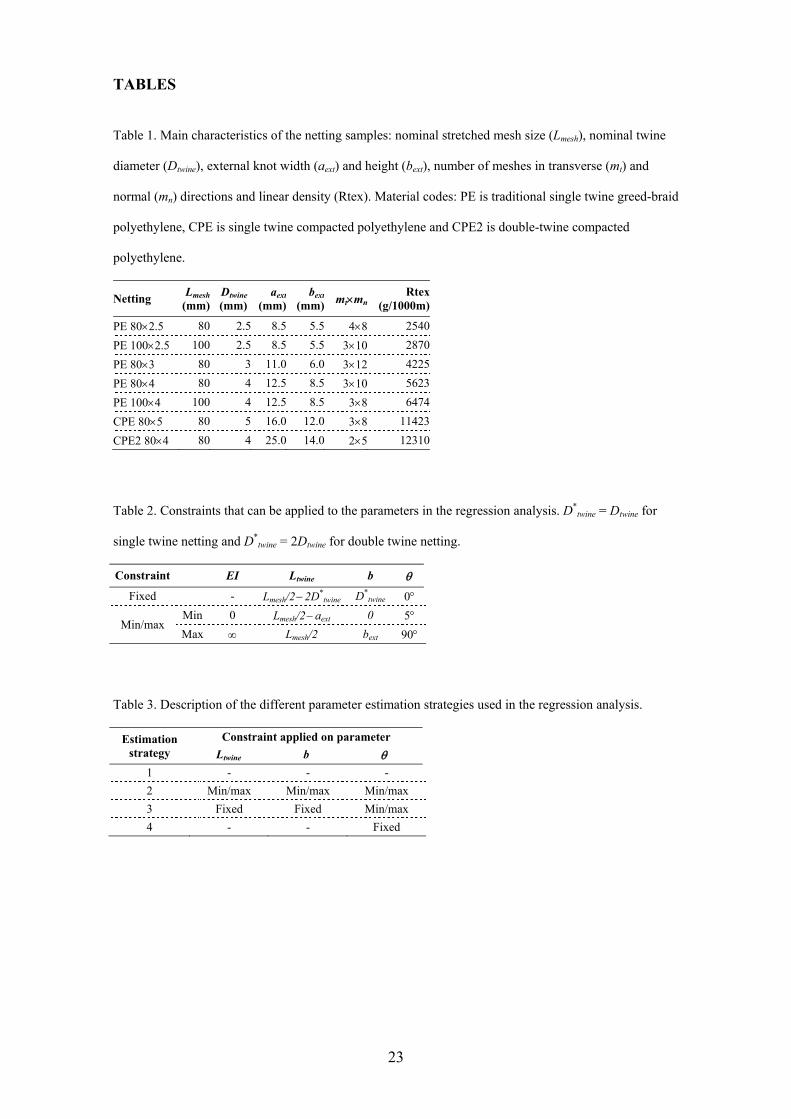
23
TABLES
Table 1. Main characteristics of the netting samples: nominal stretched mesh size (Lmesh), nominal twine
diameter (Dtwine), external knot width (aext) and height (bext), number of meshes in transverse (mt) and
normal (mn) directions and linear density (Rtex). Material codes: PE is traditional single twine greed-braid
polyethylene, CPE is single twine compacted polyethylene and CPE2 is double-twine compacted
polyethylene.
Netting Lmesh
(mm)Dtwine (mm)
aext
(mm)bext
(mm) mtmnRtex
(g/1000m)
PE 802.5 80 2.5 8.5 5.5 48 2540
PE 1002.5 100 2.5 8.5 5.5 310 2870
PE 803 80 3 11.0 6.0 312 4225
PE 804 80 4 12.5 8.5 310 5623
PE 1004 100 4 12.5 8.5 38 6474
CPE 805 80 5 16.0 12.0 38 11423
CPE2 804 80 4 25.0 14.0 25 12310
Table 2. Constraints that can be applied to the parameters in the regression analysis. D*twine = Dtwine for
single twine netting and D*twine = 2Dtwine for double twine netting.
Constraint EI Ltwine b
Fixed - Lmesh/2 2D*twine D*
twine 0
Min/max Min 0 Lmesh/2 aext 0 5
Max Lmesh/2 bext 90
Table 3. Description of the different parameter estimation strategies used in the regression analysis.
Estimation strategy
Constraint applied on parameter
Ltwine b
1 - - -
2 Min/max Min/max Min/max
3 Fixed Fixed Min/max
4 - - Fixed
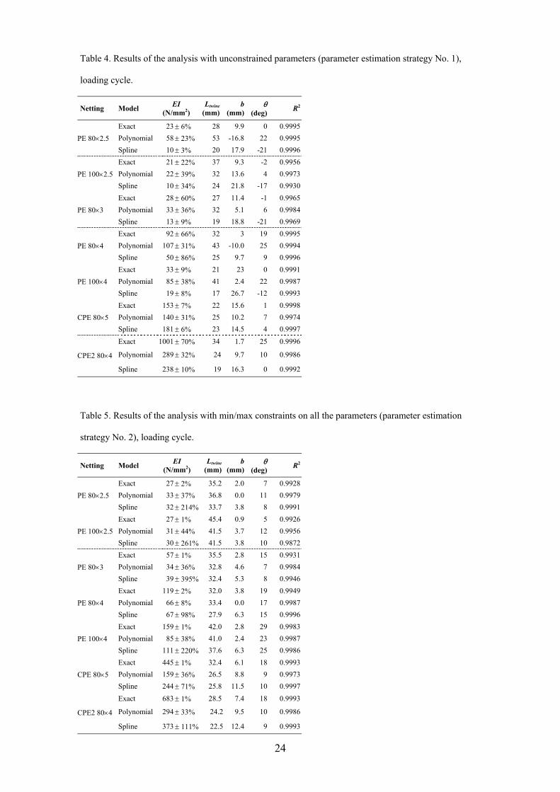
24
Table 4. Results of the analysis with unconstrained parameters (parameter estimation strategy No. 1),
loading cycle.
Netting Model EI
(N/mm2) Ltwine
(mm) b
(mm)
(deg)R2
PE 802.5
Exact 23 6% 28 9.9 0 0.9995
Polynomial 58 23% 53 -16.8 22 0.9995
Spline 10 3% 20 17.9 -21 0.9996
PE 1002.5
Exact 21 22% 37 9.3 -2 0.9956
Polynomial 22 39% 32 13.6 4 0.9973
Spline 10 34% 24 21.8 -17 0.9930
PE 803
Exact 28 60% 27 11.4 -1 0.9965
Polynomial 33 36% 32 5.1 6 0.9984
Spline 13 9% 19 18.8 -21 0.9969
PE 804
Exact 92 66% 32 3 19 0.9995
Polynomial 107 31% 43 -10.0 25 0.9994
Spline 50 86% 25 9.7 9 0.9996
PE 1004
Exact 33 9% 21 23 0 0.9991
Polynomial 85 38% 41 2.4 22 0.9987
Spline 19 8% 17 26.7 -12 0.9993
CPE 805
Exact 153 7% 22 15.6 1 0.9998
Polynomial 140 31% 25 10.2 7 0.9974
Spline 181 6% 23 14.5 4 0.9997
CPE2 804
Exact 1001 70% 34 1.7 25 0.9996
Polynomial 289 32% 24 9.7 10 0.9986
Spline 238 10% 19 16.3 0 0.9992
Table 5. Results of the analysis with min/max constraints on all the parameters (parameter estimation
strategy No. 2), loading cycle.
Netting Model EI
(N/mm2) Ltwine
(mm) b
(mm)
(deg)R2
PE 802.5
Exact 27 2% 35.2 2.0 7 0.9928
Polynomial 33 37% 36.8 0.0 11 0.9979
Spline 32 214% 33.7 3.8 8 0.9991
PE 1002.5
Exact 27 1% 45.4 0.9 5 0.9926
Polynomial 31 44% 41.5 3.7 12 0.9956
Spline 30 261% 41.5 3.8 10 0.9872
PE 803
Exact 57 1% 35.5 2.8 15 0.9931
Polynomial 34 36% 32.8 4.6 7 0.9984
Spline 39 395% 32.4 5.3 8 0.9946
PE 804
Exact 119 2% 32.0 3.8 19 0.9949
Polynomial 66 8% 33.4 0.0 17 0.9987
Spline 67 98% 27.9 6.3 15 0.9996
PE 1004
Exact 159 1% 42.0 2.8 29 0.9983
Polynomial 85 38% 41.0 2.4 23 0.9987
Spline 111 220% 37.6 6.3 25 0.9986
CPE 805
Exact 445 1% 32.4 6.1 18 0.9993
Polynomial 159 36% 26.5 8.8 9 0.9973
Spline 244 71% 25.8 11.5 10 0.9997
CPE2 804
Exact 683 1% 28.5 7.4 18 0.9993
Polynomial 294 33% 24.2 9.5 10 0.9986
Spline 373 111% 22.5 12.4 9 0.9993
25
Table 6. Results of the analysis with fixed constraints on Ltwine and b and min/max constraints on
(parameter estimation strategy No. 3), loading cycle.
Netting Model EI
(N/mm2) Ltwine
(mm) b
(mm)
(deg)R2
PE 802.5
Exact 34 1% 35 2.5 10 0.9955
Polynomial 33 6% 35 2.5 10 0.9938
Spline 35 6% 35 2.5 10 0.9990
PE 1002.5
Exact 39 2% 45 2.5 9 0.9814
Polynomial 56 24% 45 2.5 17 0.9182
Spline 77 39% 45 2.5 23 0.9464
PE 803
Exact 29 2% 34 3 5 0.9765
Polynomial 35 6% 34 3 9 0.9974
Spline 37 25% 34 3 9 0.9914
PE 804
Exact 126 3% 32 4 19 0.9920
Polynomial 99 12% 32 4 15 0.9780
Spline 126 11% 32 4 19 0.9904
PE 1004
Exact 219 2% 42 4 30 0.9873
Polynomial 164 14% 42 4 24 0.9759
Spline 218 13% 42 4 29 0.9852
CPE 805
Exact 248 2% 30 5 19 0.9914
Polynomial 198 5% 30 5 15 0.9958
Spline 273 6% 30 5 20 0.9946
CPE2 804
Exact 310 3% 24 8 18 0.9852
Polynomial 233 7% 24 8 13 0.9938
Spline 314 10% 24 8 18 0.9881
26
Table 7. Results of the analysis with fixed constraint = 0 (parameter estimation strategy No. 4), loading
cycle. Low R2 values are marked in bold font.
Netting Model EI
(N/mm2) Ltwine
(mm)b (mm) R2
PE 802.5
Exact 24 3% 28.4 9.7 0.9995
Polynomial 20 9% 27.5 9.4 0.9930
Spline 22 4% 28.1 9.4 0.9992
Asymptotic 41 10% - - 0.9936
PE 1002.5
Exact 23 17% 37.9 8.7 0.9956
Polynomial 18 6% 27.9 17.6 0.9969
Spline 19 13% 32.3 13.2 0.9896
Asymptotic 37 21% - - 0.9812
PE 803
Exact 29 8% 27.7 10.7 0.9964
Polynomial 26 6% 27.4 10.1 0.9979
Spline 27 10% 27.2 10.6 0.9952
Asymptotic 49 20% - - 0.9876
PE 804
Exact 35 4% 20.6 13.9 0.9995
Polynomial 28 12% 21.1 12.2 0.9929
Spline 33 4% 20.3 13.8 0.9996
Asymptotic 39 31% - - 0.9574
PE 1004
Exact 33 5% 21.2 23.2 0.9991
Polynomial 28 10% 21.8 21.7 0.9934
Spline 31 5% 20.9 23.1 0.9991
Asymptotic 41 31% - - 0.9656
CPE 805
Exact 148 5% 21.2 15.9 0.9998
Polynomial 97 14% 21.0 13.9 0.9960
Spline 144 5% 21.0 15.9 0.9998
Asymptotic 30 56% - - 0.7612
CPE2 804
Exact 240 11% 18.8 16.1 0.9988
Polynomial 164 13% 18.8 14.3 0.9968
Spline 233 11% 18.6 16.1 0.9989
Asymptotic 32 64% - - 0.7161
27
Table 8. Results of the analysis with min/max constraints on all the parameters (parameter estimation
strategy No. 2), unloading cycle.
Netting Model EI
(N/mm2) Ltwine
(mm) b
(mm)
(deg)R2
PE 802.5
Exact 23 0.4% 34.0 0.1 49 0.9897
Polynomial 17 195% 31.5 2.2 46 0.9798
Spline 24 219% 31.5 2.3 51 0.9873
PE 1002.5
Exact 21 1% 41.7 1.7 41 0.9871
Polynomial 15 85% 41.5 0.3 46 0.9617
Spline 49 255% 41.6 1.1 56 0.9724
PE 803
Exact 31 0.3% 35.1 0.2 50 0.9903
Polynomial 12 108% 30.6 3.8 44 0.9635
Spline 12 92% 31.2 3.2 44 0.9637
PE 804
Exact 41 0.4% 30.6 1.4 48 0.9860
Polynomial 22 78% 29.2 2.1 44 0.9907
Spline 42 137% 27.6 4.0 50 0.9930
PE 1004
Exact 107 1% 40.0 2.1 53 0.9937
Polynomial 24 53% 38.0 2.7 41 0.9917
Spline 65 132% 37.5 3.9 50 0.9947
CPE 805
Exact 80 1% 24.3 8.8 35 0.9931
Polynomial 52 117% 24.2 8.2 32 0.9971
Spline 78 600% 24.0 8.6 37 0.9963
CPE2 804
Exact 234 1% 29.0 2.8 40 0.9987
Polynomial 93 44% 23.4 7.8 30 0.9993
Spline 249 254% 31.2 0.1 43 0.9989
Table 9. Results of the analysis with fixed constraints on Ltwine and b and min/max constraints on
(parameter estimation strategy No. 3), unloading cycle.
Netting Model EI
(N/mm2) Ltwine
(mm) b
(mm)
(deg)R2
PE 802.5
Exact 264 30% 35 2.5 52 0.8343
Polynomial 433 18% 35 2.5 50 0.8563
Spline 279 31% 35 2.5 52 0.8321
PE 1002.5
Exact 752 37% 45 2.5 55 0.7635
Polynomial 853 48% 45 2.5 52 0.8490
Spline 787 37% 45 2.5 55 0.7678
PE 803
Exact 239 42% 34 3 56 0.7947
Polynomial 348 22% 34 3 54 0.8261
Spline 351 0% 34 3 59 0.8561
PE 804
Exact 535 33% 32 4 48 0.8086
Polynomial 973 26% 32 4 47 0.8482
Spline 567 35% 32 4 48 0.8054
PE 1004
Exact 712 27% 42 4 51 0.8513
Polynomial 1373 22% 42 4 50 0.8415
Spline 753 28% 42 4 51 0.8485
CPE 805
Exact 263 15% 30 5 40 0.9661
Polynomial 214 15% 30 5 35 0.9764
Spline 277 16% 30 5 40 0.9614
CPE2 804
Exact 171 6% 24 8 35 0.9975
Polynomial 133 8% 24 8 30 0.9948
Spline 182 7% 24 8 35 0.9949
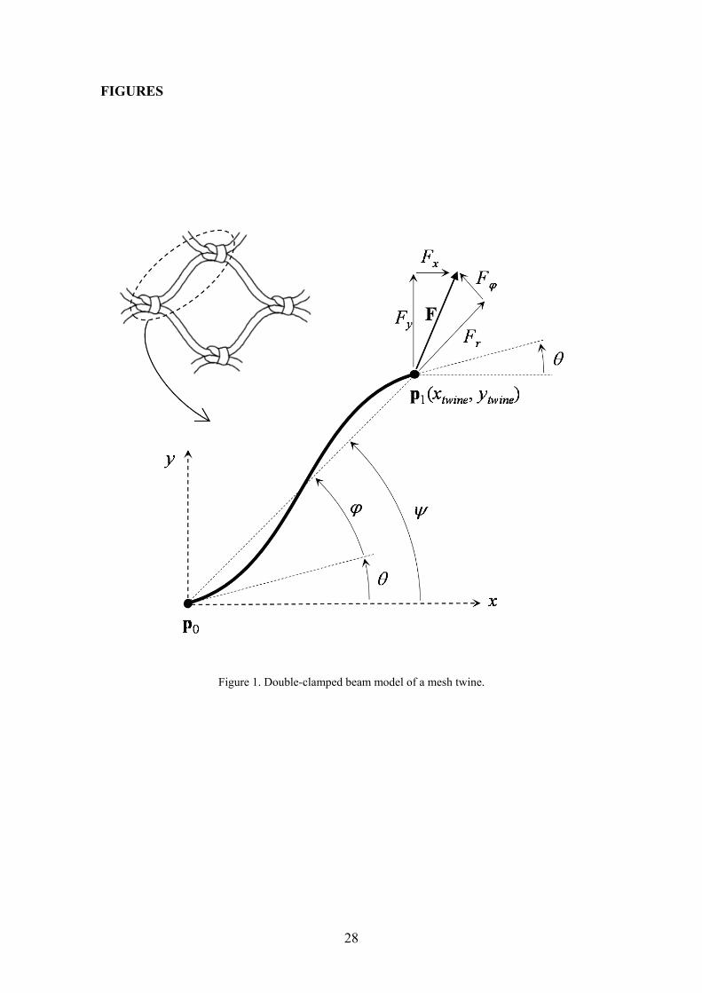
28
FIGURES
Figure 1. Double-clamped beam model of a mesh twine.
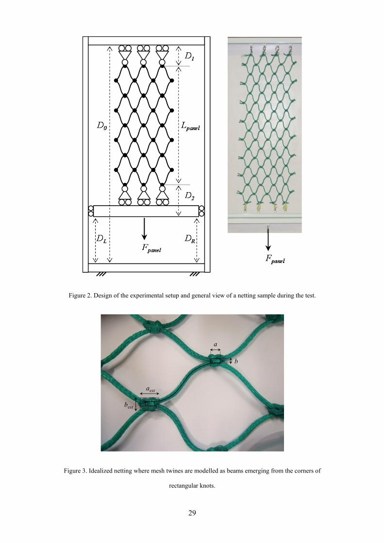
29
Figure 2. Design of the experimental setup and general view of a netting sample during the test.
Figure 3. Idealized netting where mesh twines are modelled as beams emerging from the corners of
rectangular knots.
30
Figure 4. Dimensionless vertical displacement of the twine (ytwine/Ltwine) calculated with the asymptotic
solution as a function of 22twineFLEI for different slope angles .
Figure 5. Experimental data obtained for PE 803, showing the difference between loading and unloading
cycles.
0,1
0,2
0,3
0,4
0,5
0,6
0,7
0,8
0,0 0,1 0,2 0,3 0,4 0,5
y twine/Ltwine
2
400
500
600
700
800
900
0 5 10 15 20
L panel(m
m)
Fpanel (N)
Loading
Unloading
31
Figure 6. Multiple solutions of the regression with unconstrained parameters for PE 1004, showing the
correlation between parameters in the exact and the asymptotic models: (a) bending stiffness EI versus
slope angle , (b) knot height b versus twine length Ltwine.
0
50
100
150
200
250
300
350
400
-45 -30 -15 0 15 30 45
Ben
ding
stif
fnes
s EI(
N/m
m2)
Slope angle (deg)
Asymptotic
Exact
-100
-80
-60
-40
-20
0
20
40
10 30 50 70 90 110 130 150
Kno
t hei
ght b
(mm
)
Twine length Ltwine (mm)
Asymptotic
Exact
a)
b)

32
Figure 7. Box plot of the R2 values from the parameter estimation strategies No. 2 and No. 3, loading
cycle.
Figure 8. Estimates of EI against the linear density of the netting obtained with parameter estimation
strategies No. 2 (Table 5) and No. 3 (Table 6).

Efficient and accurate methods for computational simulation of netting structures with mesh resistance to opening Ph. D. Thesis
Amelia de la Prada
Article No. 3
Assessing the suitability of gradient-based
energy minimization methods to calculate the
equilibrium shape of netting structures
Amelia de la Prada, Manuel González
Submitted to Computers and structures on 28th April 2013
Revised version submitted on 13th November 2013
Revised version submitted on 29th November 2013
Accepted for publication on 14th January 2014
Published online on 10th February 2014

Computers and Structures 135 (2014) 128–140
Contents lists available at ScienceDirect
Computers and Structures
journal homepage: www.elsevier .com/locate/compstruc
Assessing the suitability of gradient-based energy minimizationmethods to calculate the equilibrium shape of netting structures
http://dx.doi.org/10.1016/j.compstruc.2014.01.0210045-7949/� 2014 Elsevier Ltd. All rights reserved.
⇑ Corresponding author. Tel.: +34 981337400; fax: +34 981337410.E-mail addresses: [email protected] (A. de la Prada), manuel.gonzalez@
udc.es (M. González).
Amelia de la Prada, Manuel González ⇑Escuela Politécnica Superior, Universidad de A Coruña, Mendizábal s/n, 15403 Ferrol, Spain
a r t i c l e i n f o
Article history:Received 28 April 2013Accepted 14 January 2014
Keywords:Netting structuresEquilibrium shapeEnergy minimizationGradient-based optimizationNon-conservative forces
a b s t r a c t
This paper assesses the robustness and efficiency of gradient-based energy minimization methods to cal-culate the equilibrium shape of netting structures, as an alternative to the Newton–Raphson iterationthat is normally used for this purpose. A set of benchmark problems is solved to get insight on the behav-ior of different gradient-based methods and two variants of the Newton–Raphson method, using a finiteelement model of the structure. Numerical experiments indicate that the limited memory BFGS methodis generally more robust, faster, and easier to implement, and therefore it may replace or complement theNewton–Raphson method in this type of analysis.
� 2014 Elsevier Ltd. All rights reserved.
1. Introduction
Netting structures are extensively used in commercial fishingand aquaculture. The increasing concerns about the environmentalimpact and the energy efficiency in these industries have driventhe development of numerical models specially designed for thisclass of structures. They can be categorized as 1D finite elementmodels [1–3], 2D finite element models [4–6], lumped mass mod-els [7–9] and differential equation models for axisymmetric struc-tures [10,11]. Regarding the type of analysis, some applicationsrequire to calculate the dynamic behavior of the structuresubjected to water currents, waves and tides, and therefore adirect numerical integration of the equations of motion is used[7,8,12,13]. Other applications only require to calculate the staticequilibrium shape of the structure subjected to a constant watercurrent [4,11,14,15], and this work focuses in this kind of analysis.
The robustness and computational efficiency of the equilibriumshape calculation is becoming a key issue due to the recent inceptionof topology optimization of netting structures [16–18], since it isused to evaluate the objective function in such optimizations. Thenumber of function evaluations is usually high because the numberof design variables in netting structures is also high; for example, arecent iterative algorithm to optimize the energy efficiency of fish-ing gears [17] requires in the order of 104 structures which is donein 10–20 h of computing time in modern multi-core computers to
optimize a structure with 134 design variables. Methods based onheuristics (e.g. evolutionary algorithms), better suited to multi-objective optimization of netting structures, will require even morefunction evaluations and more robust calculations. Furthermore, thedesign of netting structures for fishing or aquaculture is an iterativeoptimization process, given the complexity and multidisciplinarynature of these systems: the results of a starting optimization oftenreveal problems related to factors not included in the numericalmodel (e.g. environmental impact or fish behavior), and a new opti-mization must be launched with additional constraints to avoidthem; in addition, the uncertainty in the numerical model (oceancurrents, friction with sea bottom. . .) also make necessary to launchseveral optimizations with different model parameters.
The equilibrium shapes of netting structures modeled with fi-nite elements is normally calculated by solving the equilibriumequations of the model with the Newton–Raphson method. Theaim of this work is to investigate the robustness and computationalperformance of gradient-based methods to calculate the equilib-rium shape by directly minimizing the total energy, as an alterna-tive to the Newton–Raphson iteration used in the scientificliterature. Whereas both approaches are theoretically equivalent,our hypothesis is that some gradient-based optimization methodscan outperform Newton–Raphson iteration as they do not requirematrix operations and they are not affected by ill-conditioned stiff-ness matrices which are often present in netting structures.Although energy minimization methods are usually not competi-tive for the analysis of general structures, they have proved to bea very effective method for some particular kinds of application,such as unstable trusses [19] or hyperelastic membranes [20].
A. de la Prada, M. González / Computers and Structures 135 (2014) 128–140 129
The main contribution of this work is a comprehensive assess-ment of the robustness and computational performance of bothfamilies of methods (gradient-based energy minimization andNewton iteration) to calculate the equilibrium shape of nettingstructures, in order to get insight on the advantages and disadvan-tages of each method and identify how they are affected by theparticular characteristics of the structure. The assessment is car-ried out by means of a set of benchmark problems that replicatedifferent challenging features that are present in real world appli-cations of netting structures.
The only reference in the literature to the use of energy minimi-zation methods to calculate the equilibrium shape of netting struc-tures can be found in [3], which briefly mentions the use of thePolak–Ribière version of the nonlinear conjugate gradient method.However, that work assesses neither the computational perfor-mance nor the robustness of the method in comparison to theNewton–Raphson iteration normally used in these applications.
The remaining of the paper is organized as follows: Section 2describes the numerical model of the netting structure and thesimulation methods compared in this work. Section 3 describesthe set of benchmark problems used to evaluate the performanceof the different simulation methods. In Section 4, results fromthe numerical experiments are presented and discussed. Finally,Section 5 provides conclusions and topics for future work.
2. Methods
2.1. Numerical model
The numerical model used in this work is considered the state-of-the-art for equilibrium shape calculation in netting structures[6,21,14,16–18]; a summarized description is provided here, sincedetails can be found in the references. Without loss of generality,the netting structure is supposed to be made up by panels of dia-mond mesh, the predominant netting in the fishing and aquacul-ture industry. The netting surfaces were discretized with thetriangular finite element developed in [4]. This element assumesthat all twines in each of the two directions of the netting are par-allel, and that twines behave as bars made of isotropic and linearelastic material; each node of the element has three translationaldegrees of freedom. In addition, the mesh resistance to openingis modeled as a torque proportional to the twine angle [22]. Cablesand ropes in the structure are modeled as linear bar elements [4],since their bending stiffness is negligible.
Following the same procedure as in the scientific literature[4,22], the direct formulation of the finite element method is usedinstead of the variation formulation, that is, forces are directly cal-culated from the position of the nodes in the finite element mesh.The forces applied to the model are:
(i) Elastic forces in triangular finite elements and bars, throughthe formulation described in [4,22].
(ii) Weight and buoyancy.(iii) Hydrodynamic drag forces, through the simplified expres-
sions for static analysis based on the drag forces that act ona bar under a uniform current flow [23], without taking intoaccount the fluid–structure interaction and dynamic terms[1]. The fluid velocity is projected in two components vn andvt, normal and tangential to the netting twine, which generatethe normal drag force Fn and the tangential friction force Ft, asa function of the twine length L, twine diameter d, fluid den-sity q and friction and drag coefficients Cf and Cd. For a trian-gular finite element, the total hydrodynamic force is the sumof the forces acting on all the twines in the element. The sameexpressions are used to calculate hydrodynamic forces incables and ropes discretized by bar elements:
Ft ¼12qCdLdjvt jvt
Fn ¼12qCf Ldjvnjvn
ð1Þ
Fluid–structure interaction is not considered because this topic isstill an open problem in underwater netting structures [24]. There-fore, the velocity field of the fluid is not affected by the shape of thenetting structure.
2.2. Newton iteration
The equilibrium shape of the netting structure can be obtainedby solving the equilibrium equations in the deformed configura-tion of the structure, in order to account for the large displace-ments and rotations:
FðqÞ ¼ 0 ð2Þ
where q is the nodal coordinate vector and F is the nodal force vec-tor which accumulates the contributions of the aforementionedforces. This non-linear system of equations can be solved with thewell-known Newton–Raphson (NR) iteration:
di ¼ �J�1ðqiÞFðqiÞ ð3Þ
qiþ1 ¼ qi þ kdi ð4Þ
where J is the Jacobian matrix of F, d is the search direction and k isthe step length. The classic NR method (k = 1) is not a globally con-vergent algorithm, and unfortunately the initial position of the net-ting is often numerically far from the solution. In addition, theJacobian matrix is often ill-conditioned with respect to inversion,because the in-plane stiffness of the net is several orders of magni-tude higher than the bending stiffness and the mesh opening stiff-ness; as a consequence, some iterations make a vast change in thevariables and the method does not converge. The scientific litera-ture about equilibrium shape calculation in netting structures doesnot provide details about the techniques used by other authors toovercome these issues [6,21,14,16–18]. In this work we have fol-lowed two different approaches:
The first approach is to globalize the NR iteration with a linesearch and the Armijo Rule [25,26]: for a search direction di, a suc-cession of steps lengths kj are tested until the sufficient decreasecondition is satisfied (typically a = 10�4):
jFðqi þ kjdiÞj < ð1� aÞjFðqiÞj ð5Þ
The values for kj are calculated using the three-point safeguardedparabolic model described in [25]. In addition, after five rejectedsteps (which in practice means stagnation in the iteration), the iter-ation is finished with a step length calculated with the second ap-proach. This variant of the NR method will be referred to as NRline search.
The second approach calculates the step length at each iterationwith
ki ¼kmax=maxðdiÞ if maxðdiÞ > kmax
1 otherwise
�ð6Þ
where the maximum step length per coordinate kmax is selected as afraction of the characteristic length of the netting structure; ourexperience suggests that a value about 1% is appropriated in mostsituations. We have not found references to this method in the lit-erature, but according to our experience, it often works better thanthe line search in netting structures. This variant of the NR methodwill be referred to as NR step limit.
130 A. de la Prada, M. González / Computers and Structures 135 (2014) 128–140
2.3. Gradient-based optimization methods
As an alternative to the NR method used in the literature, theauthors propose the use of gradient-based energy minimizationmethods to find the steady-state equilibrium position by minimiz-ing of the total energy of the system. The principle of minimum to-tal potential energy can be extended to system with nonconvexnonsmooth forces [27] leading to the unconstrained minimizationproblem
minq
f ðqÞ ð7Þ
where the objective function is defined as
f ðqÞ ¼ Ep �Wnc ð8Þ
where Ep represents the potential energy due to conservative forces(deformation in netting and cables, mesh opening resistance,weight and buoyancy) and Wnc represents the work carried out bynon-conservative forces acting on the system (e.g. hydrodynamicforces and friction). Wnc is calculated using a path-followingmethod [27] which allows to find the equilibrium position of non-conservative systems using energy minimization methods.With thisapproach, the gradient g of the objective function is the opposite ofthe nodal force vector F:
g ¼ rf ðqÞ ¼ �FðqÞ ð9Þ
2.3.1. Short-listing of optimization methodsGiven the large number of existing unconstrained optimization
methods [28,29], a selection process was applied in order to nar-row the scope. Optimization methods that need second-orderderivatives of the objective function (Hessian) were rejected, sincetheir evaluation would have a computational cost similar to theevaluation of the search direction di in the Newton–Raphson meth-od. Therefore, the scope was limited to methods that only needfirst-order derivative information, that is, gradient-based methods.In addition, only methods that show good performance with med-ium-large problems were selected, since problem sizes in our tar-get application are usually in the order of 102 to 104 variables.
Ten different gradient-based optimization methods were pres-elected (see Table 1), including line search methods, trust regionmethods and methods for noisy objectives. They were used to solvethe test case No. 1 described in Section 3, which is an undemandingnumerical problem. In order to reduce the development time ofthis prescreening process, publicly available implementations inMatlab programming language were used [28,30,31]; Table 1 alsolists the function name of the implementation tested for each
Table 1Shortlisted gradient-based optimization methods, the implementation refers to thefunction name in the cited reference.
Optimization method Implementation Succeed
Smooth objective:Steepest descent Steep [28]Nonlinear conjugate gradient ncg [30] XBFGS lbfgs [30] X
bfgswopt [28]fminunc [31]
Dogleg-Trust region ntrust [28]Newton-CG Trust region cgtrust [28] XTruncated Newton tn [30]
Non smooth objective:Implicit filtering imfil [28]Nelder–Mead simplex nelder [28]
fminsearch [31]Multidirectional search mds [28]Hooke–Jeeves hooke [28]
method. While these Matlab implementations may not deliverthe best computational performance, they can be used to comparethe number of function and gradient evaluations carried out tosolve the problem. Most of the methods could not solve the prob-lem in a reasonable number of function evaluations due to verypoor convergence or stagnation in the iteration, and tuning thealgorithm parameters did not improve the behavior. The only threemethods that succeeded in solving the problem are described inthe next subsections.
2.3.2. Nonlinear conjugated gradient methodThe nonlinear conjugated gradient method (CG) belongs to the
family of line search methods, where each iteration i determines asearch direction si and then minimizes f (qi + aisi) with respect tothe step length ai to generate a new iterate qi+1 = qi + aisi. CG meth-ods calculate the search direction using conjugacy properties [29].The implementation used by the authors follows the algorithmdescribed in [28]:
1. Initial position: q0
2. Evaluate f0 = f (q0), g0 = �F(q0)3. Initial approximation: s0 = �g0, i = 04. While ||gi|| > 05. Compute step length ai, set qi+1 = qi + aisi
6. Evaluate gi+1 = �F(qi+1)7. Compute bi+1
8. si+1 = �gi+1 + bi+1si
9. i = i + 110. End while11. Solution: q⁄ = qi
bi+1 in Step 7 is computed with the Polak–Ribière method, sinceit proved to be more efficient that other methods in thisapplication:
biþ1 ¼sT
iþ1ðsiþ1 � siÞsT
i si
ð10Þ
2.3.3. Limited memory BFGS methodQuasi-Newton optimization methods also follow the line search
strategy but they evaluate the search direction s for each iteration iaccording to the formula
si ¼ �H�1i gi ð11Þ
where H�1 is the inverse of the second-order derivative of f (theHessian matrix). Quasi-Newton methods estimate H with informa-tion of the gradient g and the position q. The BFGS method (Broy-den–Fletcher–Goldfarb and Shanno) estimates H with theexpression
HBFGSiþ1 ¼ Hþ 1þ cT Hc
dTc
!ddT
dTc� dcT HþHcdT
dTcð12Þ
ci ¼ giþ1 þ gi ð13Þ
di ¼ qiþ1 þ qi ð14Þ
Note that sub-index (i) has been omitted on the right-hand side ofEq. (12). Results have demonstrated that BFGS is generally the mostrobust and efficient of quasi-Newton’s methods [29]. To avoidmatrix operations and the large memory storage of the classic BFGSmethod, we selected the limited memory BFGS variant (LBFSG), thatuses the history of the iteration to compute the step without matrixoperations [28,30]; our implementation follows the algorithmdescribed in [30].
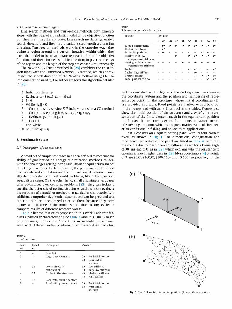
Table 3Relevant features of each test case.
Feature Test case
1 2A 2B 3A 3B 4A 4B 5 6A 6B
Large displacements – U U U U U U U U U
High initial stress – U – – – – – – – –Far initial position – U – – – – – – U –Netting with low
compression stiffness– – – U – U U U U U
Netting with very lowcompression stiffness
– – – – U U U U U U
Cables – – – – – U U – U U
Cables, high stiffness – – – – – – U – – –Ground contact – – – – – – – U U U
Panel parallel to flow – – – – – – – – U U
(a)
A. de la Prada, M. González / Computers and Structures 135 (2014) 128–140 131
2.3.4. Newton-CG Trust regionLine search methods and trust-region methods both generate
steps with the help of a quadratic model of the objective function,but they use it in different ways. Line search methods generate asearch direction, and then find a suitable step length a along thisdirection. Trust-region methods work in the opposite way: theydefine a region around the current iteration within which theytrust the model to be an adequate representation of the objectivefunction, and then choose a suitable direction; in practice, the sizeof the region and the length of the step are chosen simultaneously.
The Newton-CG Trust described in [28] combines the trust re-gion ideas with the Truncated Newton CG method, which approx-imates the search direction of the Newton method using CG. Theimplementation used by the authors follows the algorithm detailedin [28]:
1. Initial position: q0
2. Evaluate f0 = f (q0), g0 = �F(q0)3. i = 04. While ||gi|| > 05. Compute si by solving r2f (qi)si = �gi using a CG method6. Compute step length ai, set qi+1 = qi + aisi
7. Evaluate gi+1 = �F(qi+1)8. i = i + 19. End while
10. Solution: q⁄ = qi
3. Benchmark setup
3.1. Description of the test cases
A small set of simple test cases has been defined to measure theability of gradient-based energy minimization methods to dealwith the challenges arising in the calculation of equilibrium shapesof netting structures. In the literature, the performance of numer-ical models and simulation methods for netting structures is usu-ally demonstrated with real world problems, like fishing gears oraquaculture cages. On the other hand, small and simple test casesoffer advantages over complex problems [32]: they can isolate aspecific characteristic of netting structures, and therefore evaluatethe response of a model or method that particular characteristic. Inaddition, comprehensive model descriptions can be provided andother authors are encouraged to reuse them because they needto invest little time in the modelization, thus making easier tocompare results of different research works.
Table 2 list the test cases proposed in this work. Each test fea-tures a particular characteristic (see Table 3) and it is usually basedon a previous, simpler test. Some tests are available in two vari-ants, with different initial positions or stiffness values. Each test
Table 2List of test cases.
Testno.
Basedon
Description Variant
1 – Base test2 1 Large displacements 2A Far initial position
2B Near initialposition
3 2B Low stiffness incompression
3A Low stiffness3B Very low stiffness
4 3A Cables in the structure 4A Medium stiffness4B High stiffness
5 3A Rope with ground contact6 – Panel with ground contact 6A Far initial position
6B Near initialposition
will be described with a figure of the netting structure showingthe coordinate system and the position and numbering of repre-sentative points in the structure, whose initial coordinates (SI)are provided in a table. Fixed points are marked with a bold dotin the figures and with an ‘‘(f)’’ symbol in the tables. Figures alsoshow the initial position of the structure and a wireframe repre-sentation of the finite element mesh in the equilibrium position.In all tests, the structure is exposed to a constant water currentof 2 m/s in y direction, which is a representative value of the oper-ation conditions in fishing and aquaculture applications.
Test 1 consists on a square netting panel with its four cornersfixed, as shown in Fig. 1. The dimensions, configuration andmechanical properties of the panel are listed in Table 4; note thatthe couple due to mesh opening stiffness is zero for a twine angleof 30� instead of 0� as in [22], which explains why the resistance toopening is much higher than in [22]. Mesh coordinates [4] of points0–3 are (0,0), (100,0), (100,100) and (0,100) respectively. In the
(b)
Fig. 1. Test 1, base test: (a) initial position, (b) equilibrium position.
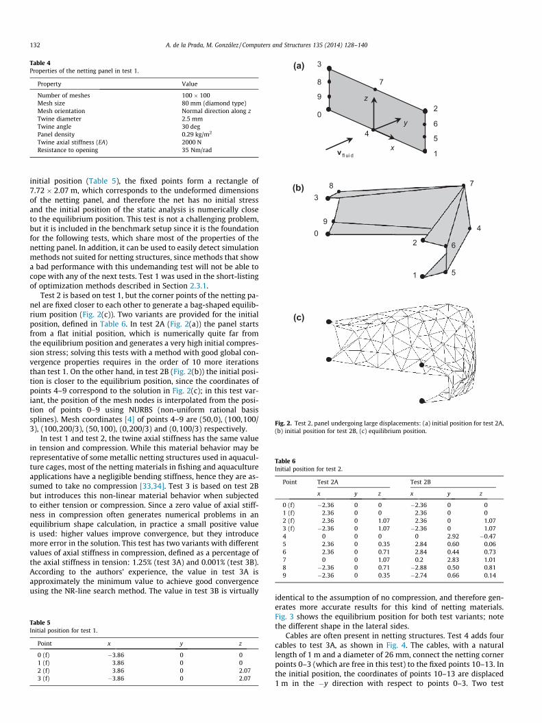
Table 4Properties of the netting panel in test 1.
Property Value
Number of meshes 100 � 100Mesh size 80 mm (diamond type)Mesh orientation Normal direction along zTwine diameter 2.5 mmTwine angle 30 degPanel density 0.29 kg/m2
Twine axial stiffness (EA) 2000 NResistance to opening 35 Nm/rad
(a)
(b)
(c)
Fig. 2. Test 2, panel undergoing large displacements: (a) initial position for test 2A,(b) initial position for test 2B, (c) equilibrium position.
Table 6Initial position for test 2.
Point Test 2A Test 2B
x y z x y z
0 (f) �2.36 0 0 �2.36 0 01 (f) 2.36 0 0 2.36 0 02 (f) 2.36 0 1.07 2.36 0 1.073 (f) �2.36 0 1.07 �2.36 0 1.074 0 0 0 0 2.92 �0.475 2.36 0 0.35 2.84 0.60 0.066 2.36 0 0.71 2.84 0.44 0.737 0 0 1.07 0.2 2.83 1.018 �2.36 0 0.71 �2.88 0.50 0.819 �2.36 0 0.35 �2.74 0.66 0.14
132 A. de la Prada, M. González / Computers and Structures 135 (2014) 128–140
initial position (Table 5), the fixed points form a rectangle of7.72 � 2.07 m, which corresponds to the undeformed dimensionsof the netting panel, and therefore the net has no initial stressand the initial position of the static analysis is numerically closeto the equilibrium position. This test is not a challenging problem,but it is included in the benchmark setup since it is the foundationfor the following tests, which share most of the properties of thenetting panel. In addition, it can be used to easily detect simulationmethods not suited for netting structures, since methods that showa bad performance with this undemanding test will not be able tocope with any of the next tests. Test 1 was used in the short-listingof optimization methods described in Section 2.3.1.
Test 2 is based on test 1, but the corner points of the netting pa-nel are fixed closer to each other to generate a bag-shaped equilib-rium position (Fig. 2(c)). Two variants are provided for the initialposition, defined in Table 6. In test 2A (Fig. 2(a)) the panel startsfrom a flat initial position, which is numerically quite far fromthe equilibrium position and generates a very high initial compres-sion stress; solving this tests with a method with good global con-vergence properties requires in the order of 10 more iterationsthan test 1. On the other hand, in test 2B (Fig. 2(b)) the initial posi-tion is closer to the equilibrium position, since the coordinates ofpoints 4–9 correspond to the solution in Fig. 2(c); in this test var-iant, the position of the mesh nodes is interpolated from the posi-tion of points 0–9 using NURBS (non-uniform rational basissplines). Mesh coordinates [4] of points 4–9 are (50,0), (100,100/3), (100,200/3), (50,100), (0,200/3) and (0,100/3) respectively.
In test 1 and test 2, the twine axial stiffness has the same valuein tension and compression. While this material behavior may berepresentative of some metallic netting structures used in aquacul-ture cages, most of the netting materials in fishing and aquacultureapplications have a negligible bending stiffness, hence they are as-sumed to take no compression [33,34]. Test 3 is based on test 2Bbut introduces this non-linear material behavior when subjectedto either tension or compression. Since a zero value of axial stiff-ness in compression often generates numerical problems in anequilibrium shape calculation, in practice a small positive valueis used: higher values improve convergence, but they introducemore error in the solution. This test has two variants with differentvalues of axial stiffness in compression, defined as a percentage ofthe axial stiffness in tension: 1.25% (test 3A) and 0.001% (test 3B).According to the authors’ experience, the value in test 3A isapproximately the minimum value to achieve good convergenceusing the NR-line search method. The value in test 3B is virtually
Table 5Initial position for test 1.
Point x y z
0 (f) �3.86 0 01 (f) 3.86 0 02 (f) 3.86 0 2.073 (f) �3.86 0 2.07
identical to the assumption of no compression, and therefore gen-erates more accurate results for this kind of netting materials.Fig. 3 shows the equilibrium position for both test variants; notethe different shape in the lateral sides.
Cables are often present in netting structures. Test 4 adds fourcables to test 3A, as shown in Fig. 4. The cables, with a naturallength of 1 m and a diameter of 26 mm, connect the netting cornerpoints 0–3 (which are free in this test) to the fixed points 10–13. Inthe initial position, the coordinates of points 10–13 are displaced1 m in the �y direction with respect to points 0–3. Two test
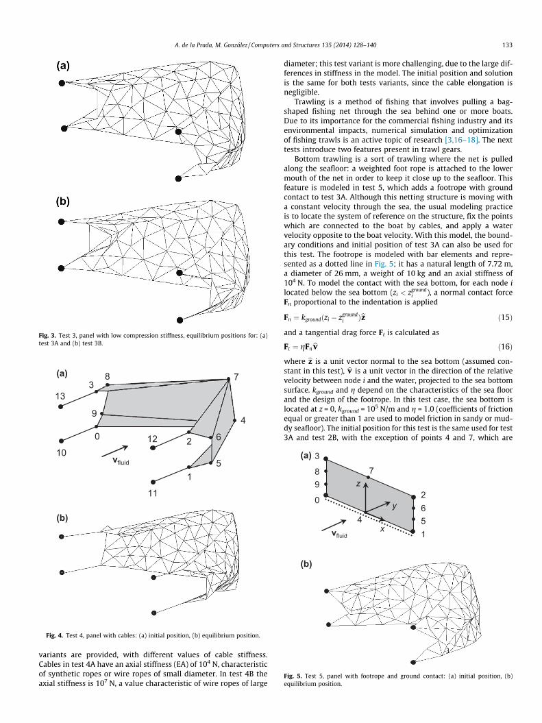
Fig. 3. Test 3, panel with low compression stiffness, equilibrium positions for: (a)test 3A and (b) test 3B.
(a)
(b)
Fig. 4. Test 4, panel with cables: (a) initial position, (b) equilibrium position.
(a)
(b)
Fig. 5. Test 5, panel with footrope and ground contact: (a) initial position, (b)equilibrium position.
A. de la Prada, M. González / Computers and Structures 135 (2014) 128–140 133
variants are provided, with different values of cable stiffness.Cables in test 4A have an axial stiffness (EA) of 104 N, characteristicof synthetic ropes or wire ropes of small diameter. In test 4B theaxial stiffness is 107 N, a value characteristic of wire ropes of large
diameter; this test variant is more challenging, due to the large dif-ferences in stiffness in the model. The initial position and solutionis the same for both tests variants, since the cable elongation isnegligible.
Trawling is a method of fishing that involves pulling a bag-shaped fishing net through the sea behind one or more boats.Due to its importance for the commercial fishing industry and itsenvironmental impacts, numerical simulation and optimizationof fishing trawls is an active topic of research [3,16–18]. The nexttests introduce two features present in trawl gears.
Bottom trawling is a sort of trawling where the net is pulledalong the seafloor: a weighted foot rope is attached to the lowermouth of the net in order to keep it close up to the seafloor. Thisfeature is modeled in test 5, which adds a footrope with groundcontact to test 3A. Although this netting structure is moving witha constant velocity through the sea, the usual modeling practiceis to locate the system of reference on the structure, fix the pointswhich are connected to the boat by cables, and apply a watervelocity opposite to the boat velocity. With this model, the bound-ary conditions and initial position of test 3A can also be used forthis test. The footrope is modeled with bar elements and repre-sented as a dotted line in Fig. 5; it has a natural length of 7.72 m,a diameter of 26 mm, a weight of 10 kg and an axial stiffness of104 N. To model the contact with the sea bottom, for each node ilocated below the sea bottom (zi < zground
i ), a normal contact forceFn proportional to the indentation is applied
Fn ¼ kgroundðzi � zgroundi Þbz ð15Þ
and a tangential drag force Ft is calculated as
Ft ¼ gFnbv ð16Þ
where bz is a unit vector normal to the sea bottom (assumed con-stant in this test), bv is a unit vector in the direction of the relativevelocity between node i and the water, projected to the sea bottomsurface. kground and g depend on the characteristics of the sea floorand the design of the footrope. In this test case, the sea bottom islocated at z = 0, kground = 105 N/m and g = 1.0 (coefficients of frictionequal or greater than 1 are used to model friction in sandy or mud-dy seafloor). The initial position for this test is the same used for test3A and test 2B, with the exception of points 4 and 7, which are
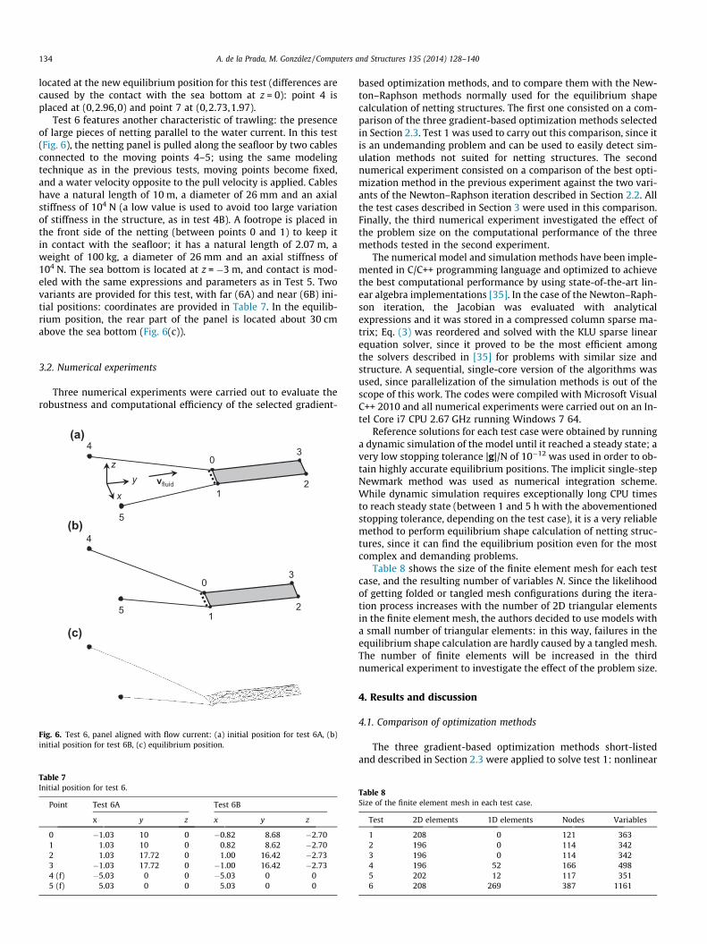
134 A. de la Prada, M. González / Computers and Structures 135 (2014) 128–140
located at the new equilibrium position for this test (differences arecaused by the contact with the sea bottom at z = 0): point 4 isplaced at (0,2.96,0) and point 7 at (0,2.73,1.97).
Test 6 features another characteristic of trawling: the presenceof large pieces of netting parallel to the water current. In this test(Fig. 6), the netting panel is pulled along the seafloor by two cablesconnected to the moving points 4–5; using the same modelingtechnique as in the previous tests, moving points become fixed,and a water velocity opposite to the pull velocity is applied. Cableshave a natural length of 10 m, a diameter of 26 mm and an axialstiffness of 104 N (a low value is used to avoid too large variationof stiffness in the structure, as in test 4B). A footrope is placed inthe front side of the netting (between points 0 and 1) to keep itin contact with the seafloor; it has a natural length of 2.07 m, aweight of 100 kg, a diameter of 26 mm and an axial stiffness of104 N. The sea bottom is located at z = �3 m, and contact is mod-eled with the same expressions and parameters as in Test 5. Twovariants are provided for this test, with far (6A) and near (6B) ini-tial positions: coordinates are provided in Table 7. In the equilib-rium position, the rear part of the panel is located about 30 cmabove the sea bottom (Fig. 6(c)).
3.2. Numerical experiments
Three numerical experiments were carried out to evaluate therobustness and computational efficiency of the selected gradient-
(a)
(b)
(c)
Fig. 6. Test 6, panel aligned with flow current: (a) initial position for test 6A, (b)initial position for test 6B, (c) equilibrium position.
Table 7Initial position for test 6.
Point Test 6A Test 6B
x y z x y z
0 �1.03 10 0 �0.82 8.68 �2.701 1.03 10 0 0.82 8.62 �2.702 1.03 17.72 0 1.00 16.42 �2.733 �1.03 17.72 0 �1.00 16.42 �2.734 (f) �5.03 0 0 �5.03 0 05 (f) 5.03 0 0 5.03 0 0
based optimization methods, and to compare them with the New-ton–Raphson methods normally used for the equilibrium shapecalculation of netting structures. The first one consisted on a com-parison of the three gradient-based optimization methods selectedin Section 2.3. Test 1 was used to carry out this comparison, since itis an undemanding problem and can be used to easily detect sim-ulation methods not suited for netting structures. The secondnumerical experiment consisted on a comparison of the best opti-mization method in the previous experiment against the two vari-ants of the Newton–Raphson iteration described in Section 2.2. Allthe test cases described in Section 3 were used in this comparison.Finally, the third numerical experiment investigated the effect ofthe problem size on the computational performance of the threemethods tested in the second experiment.
The numerical model and simulation methods have been imple-mented in C/C++ programming language and optimized to achievethe best computational performance by using state-of-the-art lin-ear algebra implementations [35]. In the case of the Newton–Raph-son iteration, the Jacobian was evaluated with analyticalexpressions and it was stored in a compressed column sparse ma-trix; Eq. (3) was reordered and solved with the KLU sparse linearequation solver, since it proved to be the most efficient amongthe solvers described in [35] for problems with similar size andstructure. A sequential, single-core version of the algorithms wasused, since parallelization of the simulation methods is out of thescope of this work. The codes were compiled with Microsoft VisualC++ 2010 and all numerical experiments were carried out on an In-tel Core i7 CPU 2.67 GHz running Windows 7 64.
Reference solutions for each test case were obtained by runninga dynamic simulation of the model until it reached a steady state; avery low stopping tolerance |g|/N of 10�12 was used in order to ob-tain highly accurate equilibrium positions. The implicit single-stepNewmark method was used as numerical integration scheme.While dynamic simulation requires exceptionally long CPU timesto reach steady state (between 1 and 5 h with the abovementionedstopping tolerance, depending on the test case), it is a very reliablemethod to perform equilibrium shape calculation of netting struc-tures, since it can find the equilibrium position even for the mostcomplex and demanding problems.
Table 8 shows the size of the finite element mesh for each testcase, and the resulting number of variables N. Since the likelihoodof getting folded or tangled mesh configurations during the itera-tion process increases with the number of 2D triangular elementsin the finite element mesh, the authors decided to use models witha small number of triangular elements: in this way, failures in theequilibrium shape calculation are hardly caused by a tangled mesh.The number of finite elements will be increased in the thirdnumerical experiment to investigate the effect of the problem size.
4. Results and discussion
4.1. Comparison of optimization methods
The three gradient-based optimization methods short-listedand described in Section 2.3 were applied to solve test 1: nonlinear
Table 8Size of the finite element mesh in each test case.
Test 2D elements 1D elements Nodes Variables
1 208 0 121 3632 196 0 114 3423 196 0 114 3424 196 52 166 4985 202 12 117 3516 208 269 387 1161
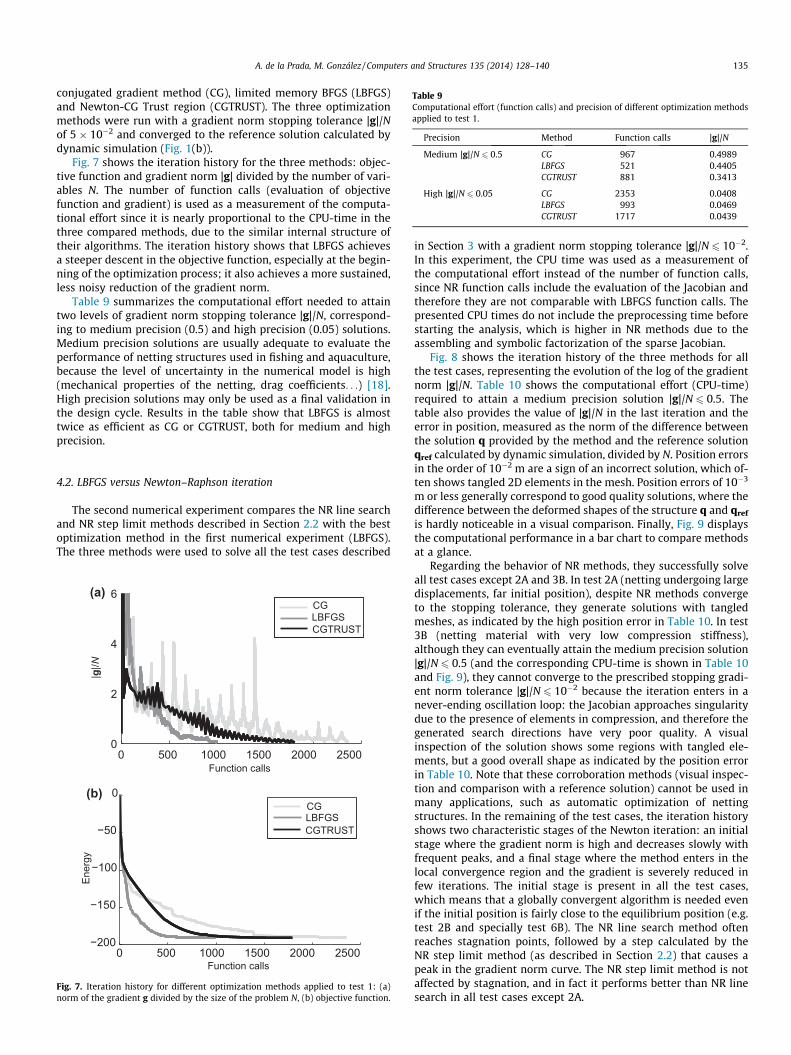
Table 9Computational effort (function calls) and precision of different optimization methodsapplied to test 1.
Precision Method Function calls |g|/N
Medium |g|/N 6 0.5 CG 967 0.4989LBFGS 521 0.4405CGTRUST 881 0.3413
High |g|/N 6 0.05 CG 2353 0.0408LBFGS 993 0.0469CGTRUST 1717 0.0439
A. de la Prada, M. González / Computers and Structures 135 (2014) 128–140 135
conjugated gradient method (CG), limited memory BFGS (LBFGS)and Newton-CG Trust region (CGTRUST). The three optimizationmethods were run with a gradient norm stopping tolerance |g|/Nof 5 � 10�2 and converged to the reference solution calculated bydynamic simulation (Fig. 1(b)).
Fig. 7 shows the iteration history for the three methods: objec-tive function and gradient norm |g| divided by the number of vari-ables N. The number of function calls (evaluation of objectivefunction and gradient) is used as a measurement of the computa-tional effort since it is nearly proportional to the CPU-time in thethree compared methods, due to the similar internal structure oftheir algorithms. The iteration history shows that LBFGS achievesa steeper descent in the objective function, especially at the begin-ning of the optimization process; it also achieves a more sustained,less noisy reduction of the gradient norm.
Table 9 summarizes the computational effort needed to attaintwo levels of gradient norm stopping tolerance |g|/N, correspond-ing to medium precision (0.5) and high precision (0.05) solutions.Medium precision solutions are usually adequate to evaluate theperformance of netting structures used in fishing and aquaculture,because the level of uncertainty in the numerical model is high(mechanical properties of the netting, drag coefficients. . .) [18].High precision solutions may only be used as a final validation inthe design cycle. Results in the table show that LBFGS is almosttwice as efficient as CG or CGTRUST, both for medium and highprecision.
4.2. LBFGS versus Newton–Raphson iteration
The second numerical experiment compares the NR line searchand NR step limit methods described in Section 2.2 with the bestoptimization method in the first numerical experiment (LBFGS).The three methods were used to solve all the test cases described
(a)
(b)
Fig. 7. Iteration history for different optimization methods applied to test 1: (a)norm of the gradient g divided by the size of the problem N, (b) objective function.
in Section 3 with a gradient norm stopping tolerance |g|/N6 10�2.In this experiment, the CPU time was used as a measurement ofthe computational effort instead of the number of function calls,since NR function calls include the evaluation of the Jacobian andtherefore they are not comparable with LBFGS function calls. Thepresented CPU times do not include the preprocessing time beforestarting the analysis, which is higher in NR methods due to theassembling and symbolic factorization of the sparse Jacobian.
Fig. 8 shows the iteration history of the three methods for allthe test cases, representing the evolution of the log of the gradientnorm |g|/N. Table 10 shows the computational effort (CPU-time)required to attain a medium precision solution |g|/N 6 0.5. Thetable also provides the value of |g|/N in the last iteration and theerror in position, measured as the norm of the difference betweenthe solution q provided by the method and the reference solutionqref calculated by dynamic simulation, divided by N. Position errorsin the order of 10�2 m are a sign of an incorrect solution, which of-ten shows tangled 2D elements in the mesh. Position errors of 10�3
m or less generally correspond to good quality solutions, where thedifference between the deformed shapes of the structure q and qref
is hardly noticeable in a visual comparison. Finally, Fig. 9 displaysthe computational performance in a bar chart to compare methodsat a glance.
Regarding the behavior of NR methods, they successfully solveall test cases except 2A and 3B. In test 2A (netting undergoing largedisplacements, far initial position), despite NR methods convergeto the stopping tolerance, they generate solutions with tangledmeshes, as indicated by the high position error in Table 10. In test3B (netting material with very low compression stiffness),although they can eventually attain the medium precision solution|g|/N 6 0.5 (and the corresponding CPU-time is shown in Table 10and Fig. 9), they cannot converge to the prescribed stopping gradi-ent norm tolerance |g|/N 6 10�2 because the iteration enters in anever-ending oscillation loop: the Jacobian approaches singularitydue to the presence of elements in compression, and therefore thegenerated search directions have very poor quality. A visualinspection of the solution shows some regions with tangled ele-ments, but a good overall shape as indicated by the position errorin Table 10. Note that these corroboration methods (visual inspec-tion and comparison with a reference solution) cannot be used inmany applications, such as automatic optimization of nettingstructures. In the remaining of the test cases, the iteration historyshows two characteristic stages of the Newton iteration: an initialstage where the gradient norm is high and decreases slowly withfrequent peaks, and a final stage where the method enters in thelocal convergence region and the gradient is severely reduced infew iterations. The initial stage is present in all the test cases,which means that a globally convergent algorithm is needed evenif the initial position is fairly close to the equilibrium position (e.g.test 2B and specially test 6B). The NR line search method oftenreaches stagnation points, followed by a step calculated by theNR step limit method (as described in Section 2.2) that causes apeak in the gradient norm curve. The NR step limit method is notaffected by stagnation, and in fact it performs better than NR linesearch in all test cases except 2A.

Fig. 8. Iteration history of different solution methods: log of the norm of the gradient g divided by the size of the problem N.
136 A. de la Prada, M. González / Computers and Structures 135 (2014) 128–140
Regarding the LBFGS method, it successfully solves all test casesexcept 4B (cables with a stiffness four orders of magnitude higherthan the netting stiffness). Its behavior in test 4B is similar to thoseof NR methods in test case 3B: the convergence is very slow, andalthough it can eventually attain the medium precision solution,it cannot converge to the prescribed stopping gradient norm toler-ance. Despite the overall position error is not high, a visual inspec-
tion of the solution shows some 2D elements in a wrong position.Additional tests were carried out to verify that the convergence ofLBFGS gets worse as the difference in stiffness values increases. Ta-ble 10 also shows a high position error for LBFGS in test 6A for atolerance |g|/N 6 0.5, but it can eventually reach the correct solu-tion at the stopping tolerance |g|/N 6 10�2. The poor computa-tional performance of LBFSG in test 6 can only be explained by
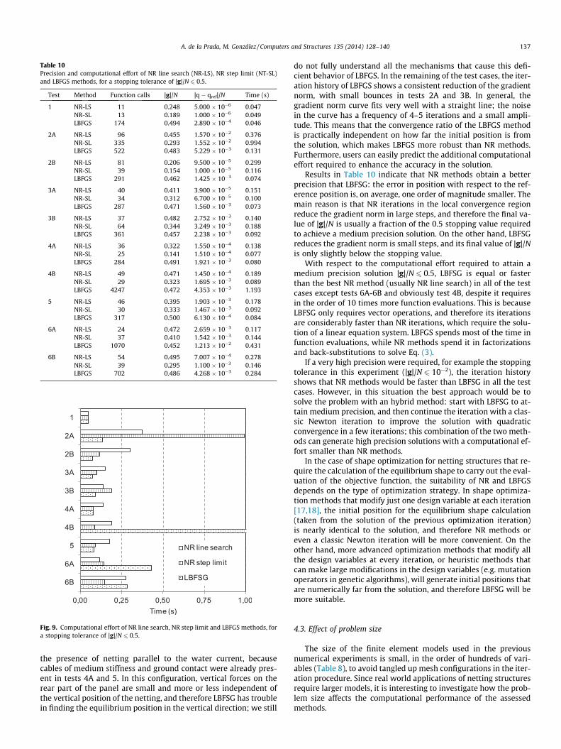
Table 10Precision and computational effort of NR line search (NR-LS), NR step limit (NT-SL)and LBFGS methods, for a stopping tolerance of |g|/N 6 0.5.
Test Method Function calls |g|/N |q � qref|/N Time (s)
1 NR-LS 11 0.248 5.000 � 10�6 0.047NR-SL 13 0.189 1.000 � 10�6 0.049LBFGS 174 0.494 2.890 � 10�4 0.046
2A NR-LS 96 0.455 1.570 � 10�2 0.376NR-SL 335 0.293 1.552 � 10�2 0.994LBFGS 522 0.483 5.229 � 10�3 0.131
2B NR-LS 81 0.206 9.500 � 10�5 0.299NR-SL 39 0.154 1.000 � 10�5 0.116LBFGS 291 0.462 1.425 � 10�3 0.074
3A NR-LS 40 0.411 3.900 � 10�5 0.151NR-SL 34 0.312 6.700 � 10�5 0.100LBFGS 287 0.471 1.560 � 10�3 0.073
3B NR-LS 37 0.482 2.752 � 10�3 0.140NR-SL 64 0.344 3.249 � 10�3 0.188LBFGS 361 0.457 2.238 � 10�3 0.092
4A NR-LS 36 0.322 1.550 � 10�4 0.138NR-SL 25 0.141 1.510 � 10�4 0.077LBFGS 284 0.491 1.921 � 10�3 0.080
4B NR-LS 49 0.471 1.450 � 10�4 0.189NR-SL 29 0.323 1.695 � 10�3 0.089LBFGS 4247 0.472 4.353 � 10�3 1.193
5 NR-LS 46 0.395 1.903 � 10�3 0.178NR-SL 30 0.333 1.467 � 10�3 0.092LBFGS 317 0.500 6.130 � 10�4 0.084
6A NR-LS 24 0.472 2.659 � 10�3 0.117NR-SL 37 0.410 1.542 � 10�3 0.144LBFGS 1070 0.452 1.213 � 10�2 0.431
6B NR-LS 54 0.495 7.007 � 10�4 0.278NR-SL 39 0.295 1.100 � 10�3 0.146LBFGS 702 0.486 4.268 � 10�3 0.284
Fig. 9. Computational effort of NR line search, NR step limit and LBFGS methods, fora stopping tolerance of |g|/N 6 0.5.
A. de la Prada, M. González / Computers and Structures 135 (2014) 128–140 137
the presence of netting parallel to the water current, becausecables of medium stiffness and ground contact were already pres-ent in tests 4A and 5. In this configuration, vertical forces on therear part of the panel are small and more or less independent ofthe vertical position of the netting, and therefore LBFSG has troublein finding the equilibrium position in the vertical direction; we still
do not fully understand all the mechanisms that cause this defi-cient behavior of LBFGS. In the remaining of the test cases, the iter-ation history of LBFGS shows a consistent reduction of the gradientnorm, with small bounces in tests 2A and 3B. In general, thegradient norm curve fits very well with a straight line; the noisein the curve has a frequency of 4–5 iterations and a small ampli-tude. This means that the convergence ratio of the LBFGS methodis practically independent on how far the initial position is fromthe solution, which makes LBFGS more robust than NR methods.Furthermore, users can easily predict the additional computationaleffort required to enhance the accuracy in the solution.
Results in Table 10 indicate that NR methods obtain a betterprecision that LBFSG: the error in position with respect to the ref-erence position is, on average, one order of magnitude smaller. Themain reason is that NR iterations in the local convergence regionreduce the gradient norm in large steps, and therefore the final va-lue of |g|/N is usually a fraction of the 0.5 stopping value requiredto achieve a medium precision solution. On the other hand, LBFSGreduces the gradient norm is small steps, and its final value of |g|/Nis only slightly below the stopping value.
With respect to the computational effort required to attain amedium precision solution |g|/N 6 0.5, LBFSG is equal or fasterthan the best NR method (usually NR line search) in all of the testcases except tests 6A-6B and obviously test 4B, despite it requiresin the order of 10 times more function evaluations. This is becauseLBFSG only requires vector operations, and therefore its iterationsare considerably faster than NR iterations, which require the solu-tion of a linear equation system. LBFGS spends most of the time infunction evaluations, while NR methods spend it in factorizationsand back-substitutions to solve Eq. (3).
If a very high precision were required, for example the stoppingtolerance in this experiment (|g|/N 6 10�2), the iteration historyshows that NR methods would be faster than LBFSG in all the testcases. However, in this situation the best approach would be tosolve the problem with an hybrid method: start with LBFSG to at-tain medium precision, and then continue the iteration with a clas-sic Newton iteration to improve the solution with quadraticconvergence in a few iterations; this combination of the two meth-ods can generate high precision solutions with a computational ef-fort smaller than NR methods.
In the case of shape optimization for netting structures that re-quire the calculation of the equilibrium shape to carry out the eval-uation of the objective function, the suitability of NR and LBFGSdepends on the type of optimization strategy. In shape optimiza-tion methods that modify just one design variable at each iteration[17,18], the initial position for the equilibrium shape calculation(taken from the solution of the previous optimization iteration)is nearly identical to the solution, and therefore NR methods oreven a classic Newton iteration will be more convenient. On theother hand, more advanced optimization methods that modify allthe design variables at every iteration, or heuristic methods thatcan make large modifications in the design variables (e.g. mutationoperators in genetic algorithms), will generate initial positions thatare numerically far from the solution, and therefore LBFSG will bemore suitable.
4.3. Effect of problem size
The size of the finite element models used in the previousnumerical experiments is small, in the order of hundreds of vari-ables (Table 8), to avoid tangled up mesh configurations in the iter-ation procedure. Since real world applications of netting structuresrequire larger models, it is interesting to investigate how the prob-lem size affects the computational performance of the assessedmethods.
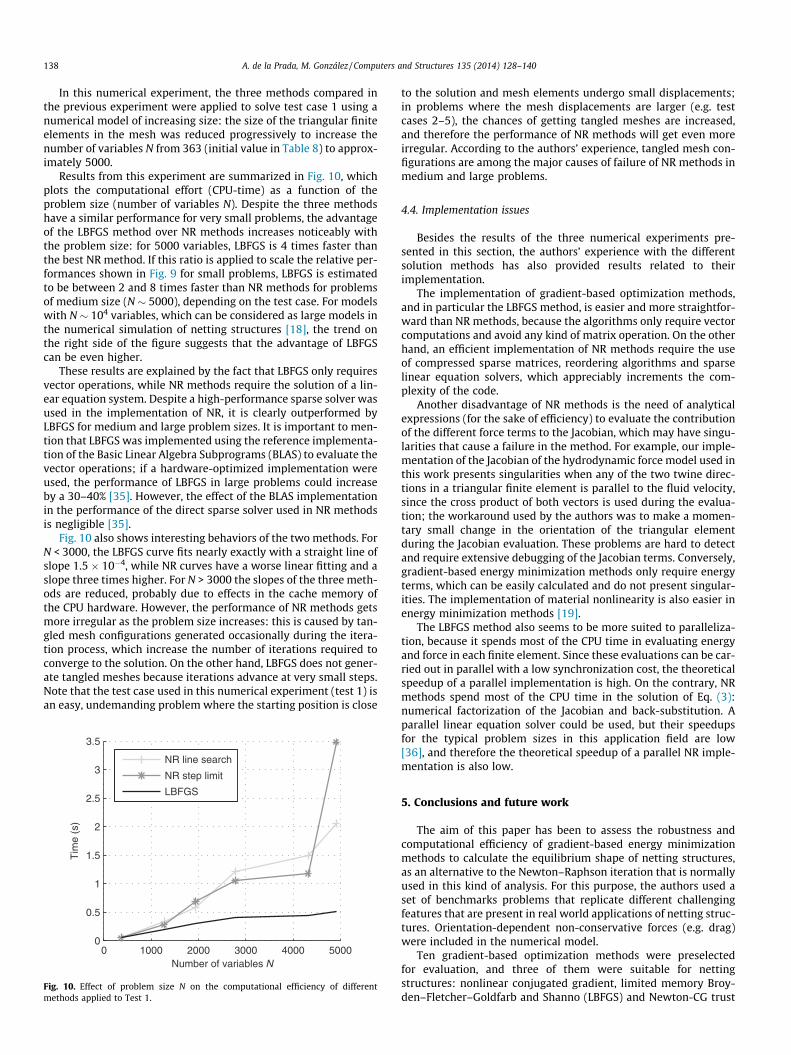
138 A. de la Prada, M. González / Computers and Structures 135 (2014) 128–140
In this numerical experiment, the three methods compared inthe previous experiment were applied to solve test case 1 using anumerical model of increasing size: the size of the triangular finiteelements in the mesh was reduced progressively to increase thenumber of variables N from 363 (initial value in Table 8) to approx-imately 5000.
Results from this experiment are summarized in Fig. 10, whichplots the computational effort (CPU-time) as a function of theproblem size (number of variables N). Despite the three methodshave a similar performance for very small problems, the advantageof the LBFGS method over NR methods increases noticeably withthe problem size: for 5000 variables, LBFGS is 4 times faster thanthe best NR method. If this ratio is applied to scale the relative per-formances shown in Fig. 9 for small problems, LBFGS is estimatedto be between 2 and 8 times faster than NR methods for problemsof medium size (N � 5000), depending on the test case. For modelswith N � 104 variables, which can be considered as large models inthe numerical simulation of netting structures [18], the trend onthe right side of the figure suggests that the advantage of LBFGScan be even higher.
These results are explained by the fact that LBFGS only requiresvector operations, while NR methods require the solution of a lin-ear equation system. Despite a high-performance sparse solver wasused in the implementation of NR, it is clearly outperformed byLBFGS for medium and large problem sizes. It is important to men-tion that LBFGS was implemented using the reference implementa-tion of the Basic Linear Algebra Subprograms (BLAS) to evaluate thevector operations; if a hardware-optimized implementation wereused, the performance of LBFGS in large problems could increaseby a 30–40% [35]. However, the effect of the BLAS implementationin the performance of the direct sparse solver used in NR methodsis negligible [35].
Fig. 10 also shows interesting behaviors of the two methods. ForN < 3000, the LBFGS curve fits nearly exactly with a straight line ofslope 1.5 � 10�4, while NR curves have a worse linear fitting and aslope three times higher. For N > 3000 the slopes of the three meth-ods are reduced, probably due to effects in the cache memory ofthe CPU hardware. However, the performance of NR methods getsmore irregular as the problem size increases: this is caused by tan-gled mesh configurations generated occasionally during the itera-tion process, which increase the number of iterations required toconverge to the solution. On the other hand, LBFGS does not gener-ate tangled meshes because iterations advance at very small steps.Note that the test case used in this numerical experiment (test 1) isan easy, undemanding problem where the starting position is close
0 1000 2000 3000 4000 50000
0.5
1
1.5
2
2.5
3
3.5
Number of variables N
Tim
e (s
)
NR line search
NR step limit
LBFGS
Fig. 10. Effect of problem size N on the computational efficiency of differentmethods applied to Test 1.
to the solution and mesh elements undergo small displacements;in problems where the mesh displacements are larger (e.g. testcases 2–5), the chances of getting tangled meshes are increased,and therefore the performance of NR methods will get even moreirregular. According to the authors’ experience, tangled mesh con-figurations are among the major causes of failure of NR methods inmedium and large problems.
4.4. Implementation issues
Besides the results of the three numerical experiments pre-sented in this section, the authors’ experience with the differentsolution methods has also provided results related to theirimplementation.
The implementation of gradient-based optimization methods,and in particular the LBFGS method, is easier and more straightfor-ward than NR methods, because the algorithms only require vectorcomputations and avoid any kind of matrix operation. On the otherhand, an efficient implementation of NR methods require the useof compressed sparse matrices, reordering algorithms and sparselinear equation solvers, which appreciably increments the com-plexity of the code.
Another disadvantage of NR methods is the need of analyticalexpressions (for the sake of efficiency) to evaluate the contributionof the different force terms to the Jacobian, which may have singu-larities that cause a failure in the method. For example, our imple-mentation of the Jacobian of the hydrodynamic force model used inthis work presents singularities when any of the two twine direc-tions in a triangular finite element is parallel to the fluid velocity,since the cross product of both vectors is used during the evalua-tion; the workaround used by the authors was to make a momen-tary small change in the orientation of the triangular elementduring the Jacobian evaluation. These problems are hard to detectand require extensive debugging of the Jacobian terms. Conversely,gradient-based energy minimization methods only require energyterms, which can be easily calculated and do not present singular-ities. The implementation of material nonlinearity is also easier inenergy minimization methods [19].
The LBFGS method also seems to be more suited to paralleliza-tion, because it spends most of the CPU time in evaluating energyand force in each finite element. Since these evaluations can be car-ried out in parallel with a low synchronization cost, the theoreticalspeedup of a parallel implementation is high. On the contrary, NRmethods spend most of the CPU time in the solution of Eq. (3):numerical factorization of the Jacobian and back-substitution. Aparallel linear equation solver could be used, but their speedupsfor the typical problem sizes in this application field are low[36], and therefore the theoretical speedup of a parallel NR imple-mentation is also low.
5. Conclusions and future work
The aim of this paper has been to assess the robustness andcomputational efficiency of gradient-based energy minimizationmethods to calculate the equilibrium shape of netting structures,as an alternative to the Newton–Raphson iteration that is normallyused in this kind of analysis. For this purpose, the authors used aset of benchmarks problems that replicate different challengingfeatures that are present in real world applications of netting struc-tures. Orientation-dependent non-conservative forces (e.g. drag)were included in the numerical model.
Ten gradient-based optimization methods were preselectedfor evaluation, and three of them were suitable for nettingstructures: nonlinear conjugated gradient, limited memory Broy-den–Fletcher–Goldfarb and Shanno (LBFGS) and Newton-CG trust
A. de la Prada, M. González / Computers and Structures 135 (2014) 128–140 139
region. Numerical experiments show that LBFGS is nearly twice asefficient as the other methods.
LBFGS was compared with two globalized variants of the New-ton–Raphson (NR) iteration: the well-known NR line search meth-od, which uses a line search and the Armijo rule as sufficientdecrease condition, and the NR step limit method that limits thestep length by a fraction of the characteristic length of the nettingstructure.
Regarding the behavior of NR methods, the following conclu-sions can be established:
– The NR step limit method performs better than the NR linesearch method in most of the problems, since it is not affectedby stagnation.
– Both methods exhibit poor convergence in netting materialswith very low compression stiffness (equal or less than 1% ofthe tension stiffness).
– Both methods have difficulty with initial positions that are farfrom the solution, since their iteration process usually generatestangled meshes which increase the computation time and mayconverge to an invalid (e.g. tangled) solution.
– Their performance gets more irregular as the problem sizeincreases, since the chances of generating a tangled mesh con-figuration during the iteration are also increased.
Regarding the LBFGS method, it has been found that it has thefollowing advantages over Newton–Raphson methods:
– It is usually faster in achieving medium precision solutions,and its advantage increases with the problem size. For prob-lems of medium size (N � 5 � 103 variables), LBFGS is esti-mated to be between 2 and 8 times faster, depending onthe type of problem. In the unusual cases where a high preci-sion solution is required, the use of LBFGS followed by a clas-sic Newton iteration is presumably faster than a globalizedNR method. Only problems with a starting position that isnearly identical to the solution make LBFGS slower than NRmethods.
– It is more robust, since it often converges to the solution at aconstant rate regardless of the goodness of the initial position,the magnitude of the displacements in the structure or the sizeof the finite element mesh. LBFGS does not suffer from stagna-tion and it avoids the generation of tangled meshes.
– It is significantly easier to implement: its algorithm avoidmatrix operations, and it does not require the error-prone eval-uation of analytical Jacobians. The lack of Jacobians also makeseasier to implement and test new force models.
– It offers more opportunities for parallelization, since it spendsmost of the computing time in function evaluations, whichcan be parallelized with high theoretical speedups.
On the other hand, LBFGS also has drawbacks. It shows verypoor convergence in problems with elements of very different stiff-ness (four orders of magnitude or more), such as soft netting struc-tures attached to wire ropes of medium or large diameter.Problems where netting panels are towed parallel to the waterflow, such in the case of bottom trawl fishing gears, also reducethe convergence ratio of the method.
The advantages of the LBFGS method suggest that is it a goodcandidate to replace or complement Newton–Raphson methodscurrently used in the equilibrium shape calculation of nettingstructures. Further research must be carried out to diminish itsdrawbacks and to verify that it also exhibits good performancewhen applied to real world applications in fishing and aquaculture.Results also show that both LBFGS and NR are several order ofmagnitude faster than dynamic simulation methods used by some
authors to find the equilibrium shape of netting structures[1,7,9,23].
In addition, the proposed set of test cases has demonstrated tobe a useful tool to assess the performance of simulation methodsfor netting structures, since it has revealed the advantages andshortcomings of the tested methods. Its simplicity also encouragesits reuse in future research, making easier to compare results fromdifferent works.
References
[1] Bessonneau JS, Marichal D. Study of the dynamics of submerged supple nets(Applications to trawls). Ocean Eng 1998;25:563–83.
[2] Tsukrov I, Eroshkin O, Fredriksson D, Swift MR, Celikkol B. Finite elementmodeling of net panels using a consistent net element. Ocean Eng2003;30:251–70.
[3] Le Dret H, Lewandowski R, Priour D, Chagneau F. Numerical simulation of a codend net. Part 1: Equilibrium in a uniform flow. J Elast 2004;76:139–62.
[4] Priour D. Calculation of net shapes by the finite element method withtriangular elements. Commun Numer Methods Eng 1999;15:755–63.
[5] Nicoll RS, Steinke DM, Attia J, Roy A, Buckham BJ. Simulation of a high-energyfinfish aquaculture site using a finite element net model. In: Proceedings of theinternational conference on offshore mechanics and arctic engineering –OMAE; 2011; p. 35–44.
[6] Priour D. Analysis of nets with hexagonal mesh using triangular elements. Int JNumer Methods Eng 2003;56:1721–33.
[7] Takagi T, Shimizu T, Suzuki K, Hiraishi T, Yamamoto K. Validity and layoutof ‘‘NaLA’’: a net configuration and loading analysis system. Fish Res2004;66:235–43.
[8] Li Y-C, Zhao Y-P, Gui F-K, Teng B. Numerical simulation of the hydrodynamicbehaviour of submerged plane nets in current. Ocean Eng 2006;33:2352–68.
[9] Lee C-W, Lee J-H, Cha B-J, Kim H-Y, Lee J-H. Physical modeling for underwaterflexible systems dynamic simulation. Ocean Eng. 2005;32:331–47.
[10] O’Neill FG. Axisymmetric trawl cod-ends made from netting of a generalizedmesh shape. IMA J Appl Math (Inst Math Appl) 1999;62:245–62.
[11] Priour D, Herrmann B, O’Neill FG. Modelling axisymmetric cod-ends made ofdifferent mesh types. Proc IMechE Part M: J Eng Maritime Env2009;223:137–44.
[12] DeCew J, Tsukrov I, Risso A, Swift MR, Celikkol B. Modeling of dynamicbehavior of a single-point moored submersible fish cage under currents.Aquacult Eng 2010;43:38–45.
[13] Lee C-W, Kim Y-B, Lee G-H, Choe M-Y, Lee M-K, Koo K-Y. Dynamic simulationof a fish cage system subjected to currents and waves. Ocean Eng2008;35:1521–32.
[14] O’Neill FG, Priour D. Comparison and validation of two models of nettingdeformation. J Appl Mech Trans ASME 2009;76:1–7.
[15] O’Neill FG, Herrmann B. PRESEMO – A predictive model of codend selectivity –a tool for fishery managers. ICES J Mar Sci 2007;64:1558–68.
[16] Priour D. Numerical optimisation of trawls design to improve their energyefficiency. Fish Res 2009;98:40–50.
[17] Khaled R, Priour D, Billard J-Y. Numerical optimization of trawl energyefficiency taking into account fish distribution. Ocean Eng 2012;54:34–45.
[18] Khaled R, Priour D, Billard J-Y. Cable length optimization for trawl fuelconsumption reduction. Ocean Eng 2013;58:167–79.
[19] Toklu Y. Nonlinear analysis of trusses through energy minimization. ComputStruct 2004;82:1581–9.
[20] Bouzidi R, van AL. Numerical solution of hyperelastic membranes by energyminimization. Comput Struct 2004;82:1961–9.
[21] Herrmann B, Priour D, Krag LA. Theoretical study of the effect of round strapson the selectivity in a diamond mesh cod-end. Fish Res 2006;80:148–57.
[22] Priour D. Introduction of mesh resistance to opening in a triangular elementfor calculation of nets by the finite element method. Commun Numer MethodsEng 2001;17:229–37.
[23] Vincent B. A new generation of tools for trawls – dynamic numericalsimulation. In: Proceedings of the fourth DEMaT workshop, Rostock; 1999.
[24] Pichot G, Germain G, Priour D. On the experimental study of the flow around afishing net. Eur. J. Mech. B/Fluids 2009;28:103–16.
[25] Kelley CT. Iterative methods for linear and nonlinearequations. Philadelphia: SIAM; 1995.
[26] Kelley CT. Solving nonlinear equations with Newton’smethod. Philadelphia: SIAM; 2003.
[27] Mistakidis ES. Nonconvex optimization in mechanics: algorithms, heuristics,and engineering applications by the F.E.M. Dordrecht; Boston: KluwerAcademic Publishers; 1998.
[28] Kelley CT. Iterative methods for optimization. Philadelphia: SIAM; 1999.[29] Fletcher R. Practical methods of optimization. Chichester, New York: Wiley;
1987.[30] Dunlavy DM, Kolda TG, Acar E. Poblano v1.0: A matlab toolbox for gradient-
based optimization. Sandia national laboratories, Albuquerque, NM andLivermore, CA; 2010.
[31] Matlab. The MathWorks Inc; 2013.[32] González M, González F, Luaces A, Cuadrado J. A collaborative benchmarking
framework for multibody system dynamics. Eng Comput 2010;26:1–9.

140 A. de la Prada, M. González / Computers and Structures 135 (2014) 128–140
[33] Moe H, Olsen A, Hopperstad OS, Jensen Ø, Fredheim A. Tensile properties fornetting materials used in aquaculture net cages. Aquacult Eng2007;37:252–65.
[34] Sala A, O’Neill FG, Buglioni G, Lucchetti A, Palumbo V, Fryer RJ. Experimentalmethod for quantifying resistance to the opening of netting panels. ICES J MarSci 2007;64:1573–8.
[35] González M, González F, Dopico D, Luaces A. On the effect of linear algebraimplementations in real-time multibody system dynamics. Comput Mech2008;41:607–15.
[36] González F, Luaces A, Lugrís U, González M. Non-intrusive parallelization ofmultibody system dynamic simulations. Comput Mech 2009;44:493–504.

Efficient and accurate methods for computational simulation of netting structures with mesh resistance to opening Ph. D. Thesis
Amelia de la Prada
Article No. 4
An efficient and accurate model for netting
structures with mesh resistance to opening
Amelia de la Prada, Manuel González
Submitted to the International Journal of Solids and Structures
on 25th April 2014

1
An efficient and accurate model for netting
structures with mesh resistance to opening
Amelia de la Prada, Manuel González*
Laboratorio de Ingeniería Mecánica Escola Politécnica Superior, Universidade da Coruña
Mendizábal s/n, 15403 Ferrol, Spain
E-mail address: [email protected], [email protected]
* Corresponding author. E-mail address: [email protected] tel.: (+34) 981337400 fax: (+34) 981337410

2
Abstract
Netting structures are extensively used in industrial fishing and aquaculture. In recent
years, there is a trend towards the use of netting materials manufactured with thicker
and stiffer twines. The increased mesh resistance to opening of such materials has a
notable impact in the structural response and performance of the structures. Several
models exist to simulate this behaviour, but they do not combine efficiency and
accuracy. This works describes a new lumped mass model for netting structures with
mesh resistance to opening. It is designed to be used in applications that only require
calculating the shape of the structure but not the stress field in the material, a common
case in marine applications. The model combines a non-linear twine beam model for
small axial deformations, a twine spring model for large axial deformations and a sphere
model for netting knots. Results of numerical and experimental validations are
presented. The model is robust, accurate and very efficient: its computational
performance is similar to linear models that do not consider mesh resistance to opening.
It shows an excellent agreement with experimental data, significantly better than
previous models described in the literature. Furthermore, it can be easily implemented
in existing computer codes for netting structures based on lumped mass methods.
Keywords: netting, resistance to opening, elastic behavior, lumped mass, equilibrium
3
1. Introduction
Flexible netting structures are extensively used in marine applications such as industrial
fishing gears and aquaculture cages. The increasing concerns about the energy
efficiency and environmental impact of these structures have driven the development of
numerical models specially designed for them. They can be categorized as 1D finite
element models (Tsukrov et al., 2003; Wan et al., 2002), 2D finite element models
(Nicoll et al., 2011; Priour, 2003, 1999), lumped mass models (Bessonneau and
Marichal, 1998; Le Dret et al., 2004; Lee et al., 2005, 2008; Li et al., 2006; Takagi et
al., 2004; Theret, 1993) and differential equation models for axisymmetric structures
(O’Neill, 1999; Priour et al., 2009). Such models have been successfully applied to
solve real-life design and optimization problems in fishing and aquaculture (DeCew et
al., 2010; Lee et al., 2011, 2011; Priour, 2009; Shimizu et al., 2007; Xu et al., 2011).
In most marine applications, the performance of a netting structure is mainly determined
by its equilibrium shape under static or quasi-static conditions. Stress or vibrations
under dynamics loads are not important in this kind of structures. For example, the
shape of a fishing trawl affects its hydrodynamic drag and its energy efficiency (Priour,
2009), and individual mesh shapes determine the size selectivity of a fishing gear
(O’Neill and Herrmann, 2007). In addition, the computational performance of the
models is becoming an important issue due to the recent inception of topology
optimization of netting structures (Khaled et al., 2012; Priour, 2009). Therefore, most
netting models focus on calculating the equilibrium position in an efficient and accurate
way, and they do not calculate stress fields in the material.
In recent years there is a trend towards the use of netting materials manufactured with
thicker and stiffer twines in order to increase the durability of the fishing gears (Sala et
4
al., 2007b). The increased mesh resistance to opening of such materials has a notable
impact in the structural response and performance of the gears. Fig. 1 illustrates the
effect of the resistance to opening in netting of diamond-oriented mesh (Fig. 1a), the
predominant material in marine applications: thicker and stiffer twines hinder mesh
opening in normal direction (Fig. 1b) compared with transverse direction (Fig. 1c). The
mesh resistance to opening is mainly characterized by the twine bending stiffness EI
(Herrmann and O’Neill, 2006; O’Neill, 2004). Theoretical and experimental studies
demonstrate that mesh resistance to opening plays as major role in the reduction of
selective performance of fishing trawls (Herrmann and O’Neill, 2006; Herrmann et al.,
2013; Lowry and Robertson, 1996; Sala et al., 2007a): an increased resistance to
opening hampers mesh opening in the codend (the aft end of fishing trawls where fish is
retained), which affects the escapement of small fish. An increased twine bending
stiffness also changes the overall shape of the fishing gear during fishing operations
(O’Neill, 2004; Priour, 2001), which has an impact on the hydrodynamic drag and thus
affects the energy efficiency of the gear (Priour, 2009). Therefore, methods to
incorporate mesh resistance to opening in numerical models of netting materials are
becoming fundamental to accurately simulate the structural response and performance
of modern flexible netting structures.
Most of the numerical models for netting materials ignore mesh resistance to opening
because they assume that twines are completely flexible and easily bent without
resistance. Only two models have been adapted to take into account this mechanical
property. Priour proposed a model based on the assumption that the couple created by
the twines on the knots varies linearly with the angle between twines (Priour, 2001).
Although this linear model can be easily included in numerical formulations, it is not
derived from any physical law and the twine bending stiffness EI is not a parameter of

5
the model. O’Neill described the equations governing the bending stiffness of a twine
and found an exact analytical solution and an asymptotic analytical solution (O’Neill,
2002). The exact solution is far too complex for practical applications. The asymptotic
solution expresses the position of the end points of the twine as an explicit function of
the tensile forces acting on it. It is only valid when the tensile forces are very high
compared to the twine bending stiffness, and it is used in the differential equation
models by the same author (O’Neill and Herrmann, 2007), which are limited to
axisymmetric structures. This asymptotic solution has drawbacks when used in more
general numerical formulations (i.e., not limited to axisymmetric structures) that need to
evaluate elastic forces in twines as a function of mesh deformation: it does not consider
twine axial elongation and it needs to be numerically inverted for every mesh element in
the model at every simulation iteration, causing a significant computational overhead.
We have recently developed a nonlinear stiffness model for a twine (de la Prada and
González, 2014a) that overcomes the drawbacks of the two abovementioned models for
mesh resistance to opening: it takes into account both axial and bending stiffness of the
twines, it is very accurate and it has a low computational overhead. This work uses that
twine stiffness model to develop an efficient and accurate model to calculate the
equilibrium position of flexible netting structures with mesh resistance to opening. The
main contributions of this work are:
(i) The twine stiffness model developed in (de la Prada and González, 2014a) is only
valid for small axial deformations. However, twines can experience very large and
unrealistic axial deformations in numerical simulations due to iterations that lead the
model through positions very far from the equilibrium (de la Prada and González,
2014b). Here we extend our twine stiffness model in order to be able to deal with such
large axial deformations.

6
(ii) Previous numerical models of netting represent knots as points and therefore neglect
their size and structure. A preliminary research with analytical axisymmetric models in
(O’Neill, 1999) demonstrate that taking into account the structure of the knots is
essential to get a good agreement between numerical and experimental results. The
numerical model presented here represents knots as spheres instead of points, and
therefore the average knot radius is taken into account in the simulations.
(iii) Previous models of netting based on the lumped mass method require eight point
masses to represent a numerical mesh: four at the knots and four at the midpoint of the
twines. The twine stiffness model used in this work avoids the need of the point masses
at the centres of the twines, thus reducing the number of degrees of freedom of the
models.
The remaining of the paper is organized as follows: Section 2 describes the numerical
model for netting structures; Section 3 presents a numerical validation, comparing the
model with a detailed finite element model and assessing its robustness and accuracy;
Section 4 presents an experimental validation of the model; Section 5 assesses the
computational efficiency of the model and compares it with a traditional formulation
which does not consider mesh resistance to opening. Finally, Sections 6 and 7 present
the discussion and the conclusions.
2. Model
2.1. Twine model for small axial deformations
The twine stiffness model used in this work was developed by the authors in (de la
Prada and González, 2014a). Based in the approach proposed in (O’Neill, 2002), a
twine is modelled as the bi-dimensional double-clamped beam shown in Fig. 2, where
7
p0 and p1 are the points where the beam attaches to the knots and 0 is the slope angle
between the twine and the knots at the insertion points. The x-axis and the y-axis are
aligned with the transverse direction and the normal direction of the mesh, respectively.
The novelty of this model is the method used to obtain the force-displacement response
of the twine. Point p0 was fixed and an enforced displacement constraint was applied to
p1 to calculate the reaction force beamf at that point by nonlinear static finite element
analysis (Zienkiewicz, 2000). The displacement constraint placed p1 on the vertices of a
rectangular curvilinear grid of size [rmin, rmax][φmin, φmax] = [0.92, 1.05] [0, π/2],
where twinetwinetwine Lyxr5.022 is the dimensionless distance between p0 and p1, twineL is
the length of the twine, 0 and twinetwine xy1tan . This grid spans all the
deformed positions that a twine can undergo in bending and moderate compression or
tension. A static analysis was run for each vertex of the grid, and dimensional analysis
and fitting techniques were applied to the obtained results to find a dimensionless model
that expresses the reaction force beamf as an explicit function of the twine deformation.
The best compromise between simplicity and accuracy consists on a polynomial surface
fitting of the polar components of the force ),( beambeamr
beam FF f as a function of the
coordinates (r, ) of p1, resulting in a polynomial degree (m, n) of (2,3) for the radial
component and (1,4) for the tangential component:
j
nmji
iij
twine
beamr rc
L
EIrF cos ,
02
(1)
j
nmji
iij
twine
beam rcL
EIrF cos ,
02
(2)
8
Coefficient values of both polynomial surfaces are provided in Table 1 and Table 2 for
three representative values of the twine axial stiffness EA in netting materials: 500 N,
1000 N and 2000 N. It was shown in (de la Prada and González, 2014a) that the effect
of EA is negligible for moderate vertical deformations of the twine ( < 48°). For larger
deformations, forces can be evaluated using three-point parabolic interpolation for a
given EA. The resulting twine stiffness model has a high goodness of fit with respect to
the finite element model, with a coefficient of determination R2 above 0.98 and a
relative error below 7%.
2.2. Twine model for large axial deformations
The twine model described in the previous subsection is only valid for deformations
within the boundaries of the rectangular curvilinear grid [rmin, rmax][φmin, φmax] used to
generate the fitting. This grid size spans all of the deformed positions that a mesh twine
can undergo in real applications of netting structures, but twines can experience larger,
unrealistic axial deformations in a numerical simulation due to iterations that lead the
model through positions very far from the equilibrium (de la Prada and González,
2014b). This is often the case when Newton iteration is used to find the equilibrium
position of the structure, particularly at the first iterations. In order to overcome this
problem, the beam model is replaced by a translational spring between p0 and p1 when
the dimensionless distance r between both points is outside the interval [rmin, rmax]. In
this way, if the twine reaches a very large axial deformation, the spring model is
activated to bring it close to the equilibrium position in a few iterations.
The translational spring force is expressed in polar components as )0,( springr
spring Ff , and
two models for springrF are considered in this work. The first one corresponds to an ideal
mechanical linear spring of natural length Ltwine:

9
)1()( rEArF springr (3)
while the second model corresponds to a spring with variable natural length, thus taking
into account the reduction in the distance between p0 and p1 as the twine bends:
))(cos()cos,( eqspring
r rrEArF (4)
where the length req(cos ) is the dimensionless radial coordinate of the trajectory
described by p1 when beamrF is zero. This trajectory was calculated in (de la Prada and
González, 2014a) as bareq cos)(cos , and the coefficients a = 0.202 and b =
0.798 are nearly independent of the twine axial stiffness EA.
To achieve a smooth transition between the beam model and the spring model, a
piecewise linear blending function α(r) is defined. Hence, the total force in the twine f(r,
) = (Fr, F) can be expressed as a composition of the forces derived from the beam
model beamf (Eq. 1 and Eq. 2) and the spring model springf (Eq. 3 or Eq. 4):
springbeamr fff )1(, (5)
Fig. 3 shows the shape of the function α(r) defined in Eq. 6. The parameter ε
determines the width of the transition region.
)( if0
)( if/)(
if1
)( if/)(
)( if0
)(
max
maxmaxmax
maxmin
minminmin
min
rr
rrrrr
rrr
rrrrr
rr
r (6)
When r < (rmin – ε) or r > (rmax + ε), the twine is highly stressed, α = 0 and the model
behaves as a spring. When rmin ≤ r ≤ rmax, the model behaves as a beam.
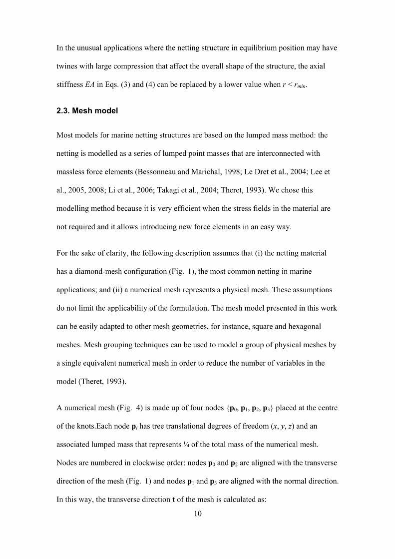
10
In the unusual applications where the netting structure in equilibrium position may have
twines with large compression that affect the overall shape of the structure, the axial
stiffness EA in Eqs. (3) and (4) can be replaced by a lower value when r < rmin.
2.3. Mesh model
Most models for marine netting structures are based on the lumped mass method: the
netting is modelled as a series of lumped point masses that are interconnected with
massless force elements (Bessonneau and Marichal, 1998; Le Dret et al., 2004; Lee et
al., 2005, 2008; Li et al., 2006; Takagi et al., 2004; Theret, 1993). We chose this
modelling method because it is very efficient when the stress fields in the material are
not required and it allows introducing new force elements in an easy way.
For the sake of clarity, the following description assumes that (i) the netting material
has a diamond-mesh configuration (Fig. 1), the most common netting in marine
applications; and (ii) a numerical mesh represents a physical mesh. These assumptions
do not limit the applicability of the formulation. The mesh model presented in this work
can be easily adapted to other mesh geometries, for instance, square and hexagonal
meshes. Mesh grouping techniques can be used to model a group of physical meshes by
a single equivalent numerical mesh in order to reduce the number of variables in the
model (Theret, 1993).
A numerical mesh (Fig. 4) is made up of four nodes {p0, p1, p2, p3} placed at the centre
of the knots.Each node pi has tree translational degrees of freedom (x, y, z) and an
associated lumped mass that represents ¼ of the total mass of the numerical mesh.
Nodes are numbered in clockwise order: nodes p0 and p2 are aligned with the transverse
direction of the mesh (Fig. 1) and nodes p1 and p3 are aligned with the normal direction.
In this way, the transverse direction t of the mesh is calculated as:
11
0202 )( ppppt (7)
Netting knots are modelled as spheres of diameter D centred at the nodes. The knots are
connected by four massless twine elements {T01, T21, T23, T03}. The ending points of the
twines pij and pji are located at the surface of the knot spheres and aligned with the
nodes pi and pj:
ijijjji
ijijiij
D
D
pppppp
pppppp
)(2
)(2 (8)
The following paragraphs describe how to evaluate the elastic forces on nodes p0 and p1
due to twine element T01. The procedure for twines T21, T23 and T03 is analogous.
A local basis {ur, u, uz} is defined for each twine Tij. Fig. 4 shows the local basis of
twine T01 (uz is not shown since it is normal to the plane of the figure). The origin of
coordinates is located on point p01, and the directions are defined as:
zr
rz
r
uuu
utu
ppppu
0101 )(
(9)
The dimensionless polar coordinates r and φ of the twine are evaluated as
00
1001
)cos(
r
twine
a
Lr
ut
pp (10)
and they are used to evaluate the twine force FFr rtwine ,, f according to Eq. 5.
The force applied by twine T01 on its ending nodes p0 and p1 can be expressed in the
local basis of the twine as
0,,
0,,
1
0
FF
FF
rtwine
rtwine
f
f (11)
12
These local forces are transformed to the global coordinate system by the twine
transformation matrix T:
zr uuuT 01 (12)
twinetwine
twinetwine
1011
0010
fTf
fTf
(13)
The total force on each node also includes the contribution of all the usual forces that
act on marine netting structures, which can be calculated with well-known methods
(Priour, 2013): hydrodynamic drag fhydro , weight fweight, buoyancy fbuoyancy and bottom
contact with the seafloor fcontact:
contacti
buoyancyi
weighti
hydroi
twineii ffffff (14)
Previous lumped mass models of netting structures use eight nodes per mesh: four at the
knots and four at the midpoint of the twines. The nodes at the midpoint of the twines are
required to simulate twine bending, because such models represent twines as bar
elements articulated in the nodes. Our model avoids the nodes in the twines because our
twine element takes into account twine bending, thus reducing the number of degrees of
freedom in the model.
As far as the knot shape is concerned, experimental methods to measure mesh resistance
to opening (Sala et al., 2007b) assume that knots are rigid rectangles of size a b and
that twines emerge from the rectangle corners (Fig. 5). Note that the rectangle size does
not match with the knot external size aext bext because in the numerical model the
twine is modelled as the central line of the real twine. This work models knots as
13
spheres of diameter D, and D can be estimated from the rectangle size a b estimated
from experimental measurements. We have found that D = (a + b) / 2 works well.
3. Numerical validation
Three numerical experiments were carried out to evaluate the accuracy and the
robustness of the numerical model described in the previous section. The test problem
used in the three experiments is based on the experimental procedure used in (Sala et
al., 2007b) to measure the mesh resistance to opening of netting panels. It consists on a
3×3 mesh netting panel that is stretched by applying simultaneous transverse and
normal loads Ft and Fn to its edges, while the transverse Lt and normal Ln mesh
openings are measured (Fig. 6). The loads and the properties of the netting panel are
taken from (Sala et al., 2007b) for traditional green-braided polyethylene 7270 Rtex:
mesh size Lmesh = 92 mm, knot size a b = 22.1 mm, EI = 345 N/mm2 and φ0 = 15.
The applied loads Ft = Fn range from 0 to 15 kg.
3.1. Comparison with a detailed finite element model
A detailed finite element model (FEM) of the test problem was built with a commercial
software (ANSYS, 2007). Each twine was discretized with 20 BEAM189 elements, a
quadratic 3D element based on Timoshenko beam theory suited for large rotation and
large strain linear applications. Knots were modelled as rigid rectangles using four
MPC184-Rigid-Beam elements. The model has 2220 nodes and 13320 degrees of
freedom. A geometric nonlinear static analysis was used to calculate the mesh openings
Lt and Ln for each value of the applied load. The test problem was also modelled with
the formulation described in the previous Section. This lumped mass model has 24
nodes and 74 degrees of freedom. The optimization method described in (de la Prada
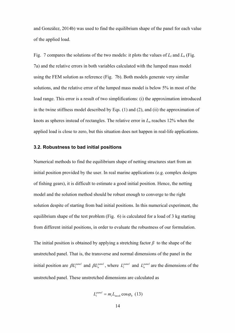
14
and González, 2014b) was used to find the equilibrium shape of the panel for each value
of the applied load.
Fig. 7 compares the solutions of the two models: it plots the values of Lt and Ln (Fig.
7a) and the relative errors in both variables calculated with the lumped mass model
using the FEM solution as reference (Fig. 7b). Both models generate very similar
solutions, and the relative error of the lumped mass model is below 5% in most of the
load range. This error is a result of two simplifications: (i) the approximation introduced
in the twine stiffness model described by Eqs. (1) and (2), and (ii) the approximation of
knots as spheres instead of rectangles. The relative error in Ln reaches 12% when the
applied load is close to zero, but this situation does not happen in real-life applications.
3.2. Robustness to bad initial positions
Numerical methods to find the equilibrium shape of netting structures start from an
initial position provided by the user. In real marine applications (e.g. complex designs
of fishing gears), it is difficult to estimate a good initial position. Hence, the netting
model and the solution method should be robust enough to converge to the right
solution despite of starting from bad initial positions. In this numerical experiment, the
equilibrium shape of the test problem (Fig. 6) is calculated for a load of 3 kg starting
from different initial positions, in order to evaluate the robustness of our formulation.
The initial position is obtained by applying a stretching factor β to the shape of the
unstretched panel. That is, the transverse and normal dimensions of the panel in the
initial position are paneltL and panel
nL , where paneltL and panel
nL are the dimensions of the
unstretched panel. These unstretched dimensions are calculated as
0cosmeshtpanelt LmL (13)
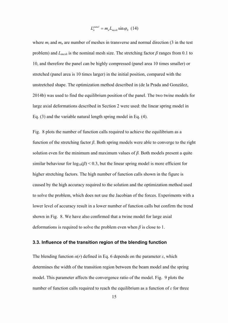
15
0sinmeshnpaneln LmL (14)
where mt and mn are number of meshes in transverse and normal direction (3 in the test
problem) and Lmesh is the nominal mesh size. The stretching factor β ranges from 0.1 to
10, and therefore the panel can be highly compressed (panel area 10 times smaller) or
stretched (panel area is 10 times larger) in the initial position, compared with the
unstretched shape. The optimization method described in (de la Prada and González,
2014b) was used to find the equilibrium position of the panel. The two twine models for
large axial deformations described in Section 2 were used: the linear spring model in
Eq. (3) and the variable natural length spring model in Eq. (4).
Fig. 8 plots the number of function calls required to achieve the equilibrium as a
function of the stretching factor β. Both spring models were able to converge to the right
solution even for the minimum and maximum values of β. Both models present a quite
similar behaviour for log10(β) < 0.3, but the linear spring model is more efficient for
higher stretching factors. The high number of function calls shown in the figure is
caused by the high accuracy required to the solution and the optimization method used
to solve the problem, which does not use the Jacobian of the forces. Experiments with a
lower level of accuracy result in a lower number of function calls but confirm the trend
shown in Fig. 8. We have also confirmed that a twine model for large axial
deformations is required to solve the problem even when β is close to 1.
3.3. Influence of the transition region of the blending function
The blending function α(r) defined in Eq. 6 depends on the parameter ε, which
determines the width of the transition region between the beam model and the spring
model. This parameter affects the convergence ratio of the model. Fig. 9 plots the
number of function calls required to reach the equilibrium as a function of ε for three

16
different initial positions (stretching factor β = 1, 2, 3). Numerical experiments for
higher values of β were carried out, but results are not shown since they follow the trend
in Fig. 9. The influence of ε becomes noticeable when β > 2: the number of function
calls always increases for ε < 0.03 and ε > 0.05, regardless of the value of β. Therefore,
a value of ε = 0.04 is recommended.
4. Experimental validation
A simple experiment (Fig. 10) was carried out to verify that the model presented in this
work can predict the mesh resistance to opening of a real netting material. A 38 mesh
polyethylene panel was hold between an upper fixed bar and a bottom free bar. The
panel was stretched in the normal direction of the meshes by applying a growing force
panelF to the bottom bar and the resulting length of the panel panelL was measured. The
experimental data was analyzed with the method proposed in (Sala et al., 2007b) to
estimate the mechanical and dimensional parameters of the netting sample. The method
uses nonlinear least squares regression to fit a theoretical model for mesh resistance to
opening to the experimental data. In this example, the model function used in the
regression analysis was a computer implementation of the netting model described in
Section 2, particularized for a 38 mesh panel to match the dimensions of the sample
used in the experiment. Four parameters of the model were estimated: the twine bending
stiffness EI, the twine length Ltwine, the diameter D of the knot spheres and the angle φ0.
The nonlinear regression provides the following estimates and confidence intervals for
the parameters: EI = 74.9 ± 8.7 % N/mm2, Ltwine = 41.5 ± 2.6 % mm, D = 2.1 ± 0.7%
mm and φ0 = 22.7 ± 0.4%. Fig. 11 plots the length of the panel panelL as a function of
the applied force panelF . The values of panelL predicted by the fitted model are
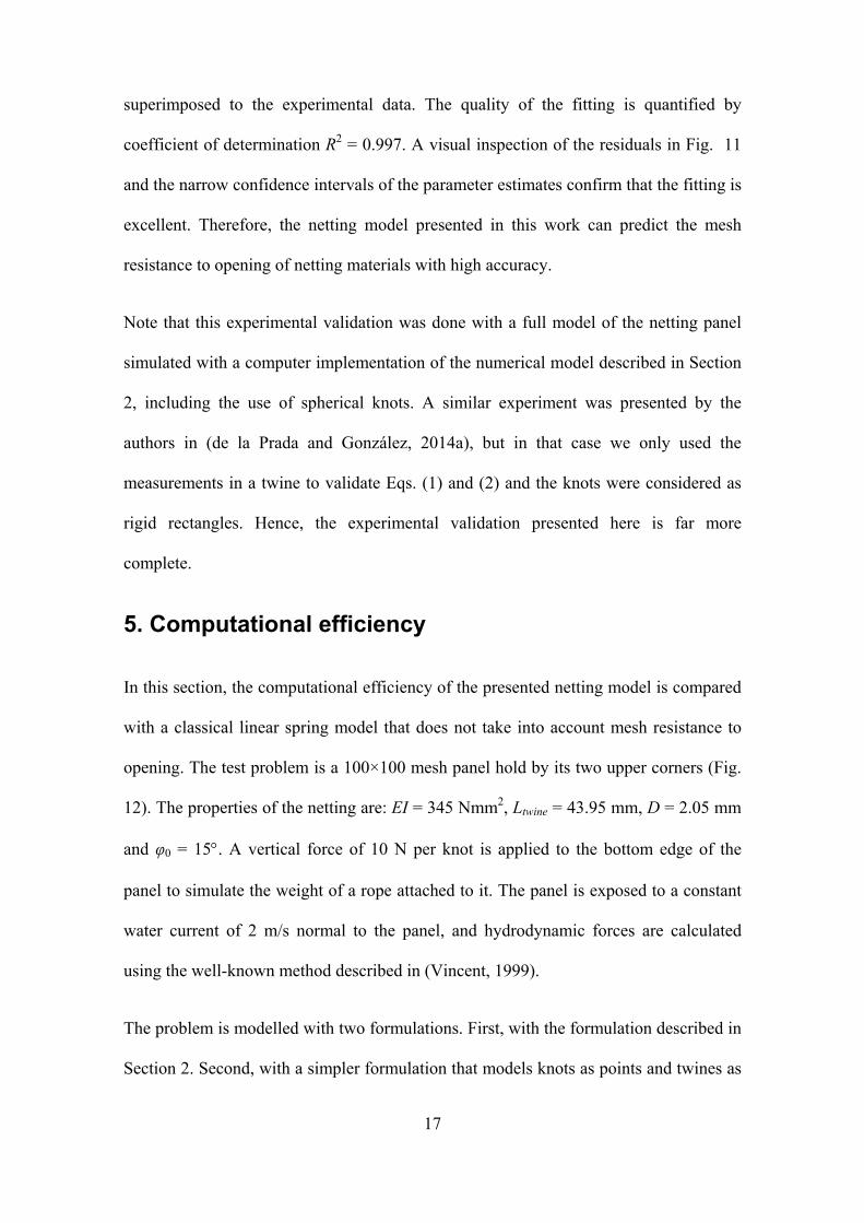
17
superimposed to the experimental data. The quality of the fitting is quantified by
coefficient of determination R2 = 0.997. A visual inspection of the residuals in Fig. 11
and the narrow confidence intervals of the parameter estimates confirm that the fitting is
excellent. Therefore, the netting model presented in this work can predict the mesh
resistance to opening of netting materials with high accuracy.
Note that this experimental validation was done with a full model of the netting panel
simulated with a computer implementation of the numerical model described in Section
2, including the use of spherical knots. A similar experiment was presented by the
authors in (de la Prada and González, 2014a), but in that case we only used the
measurements in a twine to validate Eqs. (1) and (2) and the knots were considered as
rigid rectangles. Hence, the experimental validation presented here is far more
complete.
5. Computational efficiency
In this section, the computational efficiency of the presented netting model is compared
with a classical linear spring model that does not take into account mesh resistance to
opening. The test problem is a 100×100 mesh panel hold by its two upper corners (Fig.
12). The properties of the netting are: EI = 345 Nmm2, Ltwine = 43.95 mm, D = 2.05 mm
and φ0 = 15. A vertical force of 10 N per knot is applied to the bottom edge of the
panel to simulate the weight of a rope attached to it. The panel is exposed to a constant
water current of 2 m/s normal to the panel, and hydrodynamic forces are calculated
using the well-known method described in (Vincent, 1999).
The problem is modelled with two formulations. First, with the formulation described in
Section 2. Second, with a simpler formulation that models knots as points and twines as

18
linear springs, ignoring the effect of mesh resistance to opening and the knot structure.
This second formulation is very similar to the lumped mass netting models developed
by other authors (Bessonneau and Marichal, 1998; Le Dret et al., 2004; Lee et al., 2005,
2008; Li et al., 2006; Takagi et al., 2004; Theret, 1993), but in this case we do not use
nodes in the midpoints of twines in order to be able to share the numerical mesh grid
between both models. For simplicity, each physical mesh is modelled with a numerical
mesh in both models: the problem has 104 numerical meshes, 20604 nodes and 61812
variables.
The equilibrium position shown in Fig. 12 was calculated with the same optimization
method used in Section 3 (de la Prada and González, 2014b), imposing a stopping
tolerance of 10-3 to achieve a highly accurate solution. The results obtained with the two
models are visibly different. Table 3 summarizes the computational performance of both
models. The solution time and the number of force evaluations are high because the
initial position was far from the equilibrium, a very fine mesh grid was used and a small
tolerance was required. In practical applications, a coarse mesh grid would be used in
the first iterations, thus reducing the total computing time in about two orders of
magnitude. The key performance indicator is the time per force evaluation in a
numerical mesh (the last row in Table 3), which includes the evaluation of all non-
constant forces (twine elastic forces and hydrodynamic drag). The model presented in
this work does not affect the number of iterations, but it is twice as slow as the classical
linear spring model without mesh resistance to opening.
A clarification is necessary to interpret this result. The classical linear spring model
used in this comparison does not have nodes in the midpoints of twines, as explained
before. But such nodes are used in all lumped mass models for netting structures
(Bessonneau and Marichal, 1998; Le Dret et al., 2004; Lee et al., 2005, 2008; Li et al.,

19
2006; Takagi et al., 2004; Theret, 1993) to describe the curvature of the twine. The
midpoint nodes duplicate the number of linear springs in a numerical mesh (from 4 to
8), and therefore they increase the time per force evaluation in a mesh in a factor about
two. This means that the computational efficiency of the model presented in this work is
similar to previous lumped mass models that do not consider mesh resistance to
opening. Note that the presented model does not need nodes in the midpoints of the
twines to take into account twine bending, since it is already considered in the beam
model described by Eqs. (1) and (2).
6. Discussion
The results of the numerical validation show that the presented model is robust and has
a good accuracy compared to a detailed finite element model. The differences with the
finite element model (relative errors below 5%) are not important due to the high
uncertainty in the mechanical properties of netting materials for marine applications,
which change during use (Sala et al., 2004). Moreover, the detailed finite element model
used in Section 3 is an approximation of the real structure of the netting: real twines are
likely to have a very complex behavior due to the structure its polymer fibers, and real
knots are not completely rigid structures.
The results of the experimental validation are far better than the results presented in
(Sala et al., 2007b), which used a similar experiment to quantify the mesh resistance to
opening of netting panels. The asymptotic model developed in (O’Neill, 2002) was used
in that work to analyze experimental data, and the authors reported a systematic lack of
fit of their model to the experimental data and identifiability problems in the parameters
of the model. On the contrary, our model provides an excellent goodness of fit and
parameter estimates with narrow confidence intervals. This suggests that the model

20
presented in this work could be also used to quantify the mesh resistance to opening of
netting panels in a more reliable way than in (Sala et al., 2007b).
The approximation of knots as spheres instead of rectangles seems to have little effect in
the experimental validation presented in this work. However, knots in other kind of
netting materials may have the shape of a rectangle with a large aspect ratio, and
therefore the sphere approximation may provide worse agreement with experimental
data in such materials. More research is required to get insight about this topic. If
required, the presented netting model could be easily modified to consider knots as
rectangular parallelepipeds.
A major objection to the netting model presented in this work is that it does not consider
the twine flexion outside the plane of the netting. This is the usual practice in all the
netting models for marine applications, since the curvature of marine netting structures
is small and therefore the moment generated by the out-of-plane bending can be
neglected. In our netting model, this simplification is present in the mesh model
described in Section 2, which implicitly assumes that twines are contained in the plane
defined by its ending knots and the transverse direction of the mesh. However, out-of-
plane bending modifies the shape of the twines and hence it may modify the resistance
to opening of the netting. This issue has not been investigated yet in the literature.
Further experimental work is required to verify the accuracy of the presented netting
model when out-of-plane bending is present. This matter is out of the scope of this
article due to the complexity of the required experimental work.

21
7. Conclusions
A lumped mass model for netting structures with mesh resistance to opening is
presented. It is designed to be used in applications that only require calculating the
shape of the structures but not the stress fields in the material. This is the case of many
marine applications of netting structures (e.g. fishing gears). The model combines a
twine beam model for small axial deformations, a twine spring model for large axial
deformations and a sphere model for netting knots. The model has significant
advantages over previous methods to simulate the resistance to opening in netting
materials. Numerical experiments confirmed that it is very robust. It also shows an
excellent agreement with experimental data. Despite the higher non-linearity of this
model, its computational performance is similar to other models that do not consider
mesh resistance to opening because it avoids nodes in the midpoints of twines. The
model can be easily implemented in existing computer codes that use other lumped
mass models for netting structures.
The presented model will be very useful to improve the designs of certain marine
netting structures. For example, the design of selective fishing gears is a very active
research field that requires predicting the selectivity of the gear using behavioral models
of fish and structural models of netting (O’Neill and Herrmann, 2007). Accurate
simulation of mesh opening in the gear is essential for these methods, and the model
presented in this work can achieve such accuracy when thicker and stiffer twines are
used. Another application of the presented model is the experimental quantification of
the mesh resistance to opening of netting materials, as an alternative to the method
described in (Sala et al., 2007b): the model can be fitted to experimental data using non-

22
linear regression in order to obtain an accurate estimation of the mechanical and
dimensional parameters that govern the resistance to opening.
Finally, further research is needed to verify that the model is still valid with out-of-plane
bending is present in the netting material. Despite out-of-plane bending is neglected in
netting models for marine applications due to the low curvature of the netting structures,
it may affect the resistance to opening of the netting.
23
References
ANSYS, 2007. . ANSYS, Inc. Bessonneau, J.S., Marichal, D., 1998. Study of the dynamics of submerged supple nets. (Applications to
trawls). Ocean Eng. 25, 563–583. De la Prada, A., González, M., 2014a. Nonlinear stiffness models of a net twine to describe mesh
resistance to opening of flexible net structures. Proc. Inst. Mech. Eng. Part M J. Eng. Marit. Environ. In press. doi:10.1177/1475090214530876, proof available at http://lim.ii.udc.es/tmp/PIM530876.pdf
De la Prada, A., González, M., 2014b. Assessing the suitability of gradient-based energy minimization methods to calculate the equilibrium shape of netting structures. Comput. Struct. 135, 128–140. doi:10.1016/j.compstruc.2014.01.021
DeCew, J., Tsukrov, I., Risso, A., Swift, M.R., Celikkol, B., 2010. Modeling of dynamic behavior of a single-point moored submersible fish cage under currents. Aquac. Eng. 43, 38–45.
Herrmann, B., O’Neill, F.G., 2006. Theoretical study of the influence of twine thickness on haddock selectivity in diamond mesh cod-ends. Fish. Res. 80, 221–229.
Herrmann, B., Wienbeck, H., Moderhak, W., Stepputtis, D., Krag, L.A., 2013. The influence of twine thickness, twine number and netting orientation on codend selectivity. Fish. Res. 145, 22–36.
Khaled, R., Priour, D., Billard, J.-Y., 2012. Numerical optimization of trawl energy efficiency taking into account fish distribution. Ocean Eng. 54, 34–45.
Le Dret, H., Lewandowski, R., Priour, D., Chagneau, F., 2004. Numerical simulation of a cod end net part 1: Equilibrium in a uniform flow. J. Elast. 76, 139–162.
Lee, C.-W., Lee, J.-H., Cha, B.-J., Kim, H.-Y., Lee, J.-H., 2005. Physical modeling for underwater flexible systems dynamic simulation. Ocean Eng. 32, 331–347.
Lee, J., Lee, C.-W., Choe, M.-Y., Lee, G.-H., 2011. Applying fishing-gear simulation software to better estimate fished space as fishing effort. Fish. Aquat. Sci. 14, 138–147.
Lee, J.H., Karlsen, L., Lee, C.W., 2008. A method for improving the dynamic simulation efficiency of underwater flexible structures by implementing non-active points in modelling. ICES J. Mar. Sci. 65, 1552–1558.
Li, Y.-C., Zhao, Y.-P., Gui, F.-K., Teng, B., 2006. Numerical simulation of the hydrodynamic behaviour of submerged plane nets in current. Ocean Eng. 33, 2352–2368.
Lowry, N., Robertson, J.H.B., 1996. The effect of twine thickness on cod-end selectivity of trawls for haddock in the North Sea. Fish. Res. 26, 353–363.
Nicoll, R.S., Steinke, D.M., Attia, J., Roy, A., Buckham, B.J., 2011. Simulation of a high-energy finfish aquaculture site using a finite element net model, in: Proceedings of the International Conference on Offshore Mechanics and Arctic Engineering - OMAE. pp. 35–44.
O’Neill, F.G., 1999. Axisymmetric trawl cod-ends made from netting of a generalized mesh shape. IMA J. Appl. Math. Inst. Math. Its Appl. 62, 245–262.
O’Neill, F.G., 2002. Bending of twines and fibres under tension. J. Text. Inst. 93, 1–8. O’Neill, F.G., 2004. The Influence of Bending Stiffness on the Deformation of Axisymmetric Networks,
in: ASME 2004 23rd International Conference on Offshore Mechanics and Arctic Engineering. ASME, pp. 749–754. doi:10.1115/OMAE2004-51421
O’Neill, F.G., Herrmann, B., 2007. PRESEMO - A predictive model of codend selectivity - A tool for fishery managers. ICES J. Mar. Sci. 64, 1558–1568. doi:10.1093/icesjms/fsm101
Priour, D., 1999. Calculation of net shapes by the finite element method with triangular elements. Commun. Numer. Methods Eng. 15, 755–763.
Priour, D., 2001. Introduction of mesh resistance to opening in a triangular element for calculation of nets by the finite element method. Commun. Numer. Methods Eng. 17, 229–237.
Priour, D., 2003. Analysis of nets with hexagonal mesh using triangular elements. Int. J. Numer. Methods Eng. 56, 1721–1733.
Priour, D., 2009. Numerical optimisation of trawls design to improve their energy efficiency. Fish. Res. 98, 40–50.
Priour, D., 2013. A finite element method for netting. Springer, New York. Priour, D., Herrmann, B., O’Neill, F.G., 2009. Modelling axisymmetric cod-ends made of different mesh
types. Proc. Inst. Mech. Eng. Part M J. Eng. Marit. Environ. 223, 137–144. Sala, A., Lucchetti, A., Buglioni, G., 2004. The change in physical properties of some nylon (PA) netting
samples before and after use. Fish. Res. 69, 181–188.
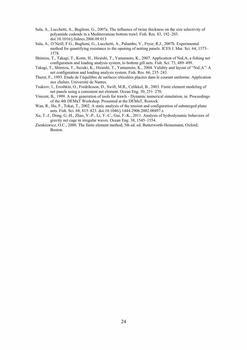
24
Sala, A., Lucchetti, A., Buglioni, G., 2007a. The influence of twine thickness on the size selectivity of polyamide codends in a Mediterranean bottom trawl. Fish. Res. 83, 192–203. doi:10.1016/j.fishres.2006.09.013
Sala, A., O’Neill, F.G., Buglioni, G., Lucchetti, A., Palumbo, V., Fryer, R.J., 2007b. Experimental method for quantifying resistance to the opening of netting panels. ICES J. Mar. Sci. 64, 1573–1578.
Shimizu, T., Takagi, T., Korte, H., Hiraishi, T., Yamamoto, K., 2007. Application of NaLA, a fishing net configuration and loading analysis system, to bottom gill nets. Fish. Sci. 73, 489–499.
Takagi, T., Shimizu, T., Suzuki, K., Hiraishi, T., Yamamoto, K., 2004. Validity and layout of “NaLA”: A net configuration and loading analysis system. Fish. Res. 66, 235–243.
Theret, F., 1993. Etude de l’équilibre de surfaces réticulées placées dans le courant uniforme. Application aux chaluts. Université de Nantes.
Tsukrov, I., Eroshkin, O., Fredriksson, D., Swift, M.R., Celikkol, B., 2003. Finite element modeling of net panels using a consistent net element. Ocean Eng. 30, 251–270.
Vincent, B., 1999. A new generation of tools for trawls - Dynamic numerical simulation, in: Proceedings of the 4th DEMaT Workshop. Presented at the DEMaT, Rostock.
Wan, R., Hu, F., Tokai, T., 2002. A static analysis of the tension and configuration of submerged plane nets. Fish. Sci. 68, 815–823. doi:10.1046/j.1444-2906.2002.00497.x
Xu, T.-J., Dong, G.-H., Zhao, Y.-P., Li, Y.-C., Gui, F.-K., 2011. Analysis of hydrodynamic behaviors of gravity net cage in irregular waves. Ocean Eng. 38, 1545–1554.
Zienkiewicz, O.C., 2000. The finite element method, 5th ed. ed. Butterworth-Heinemann, Oxford; Boston.
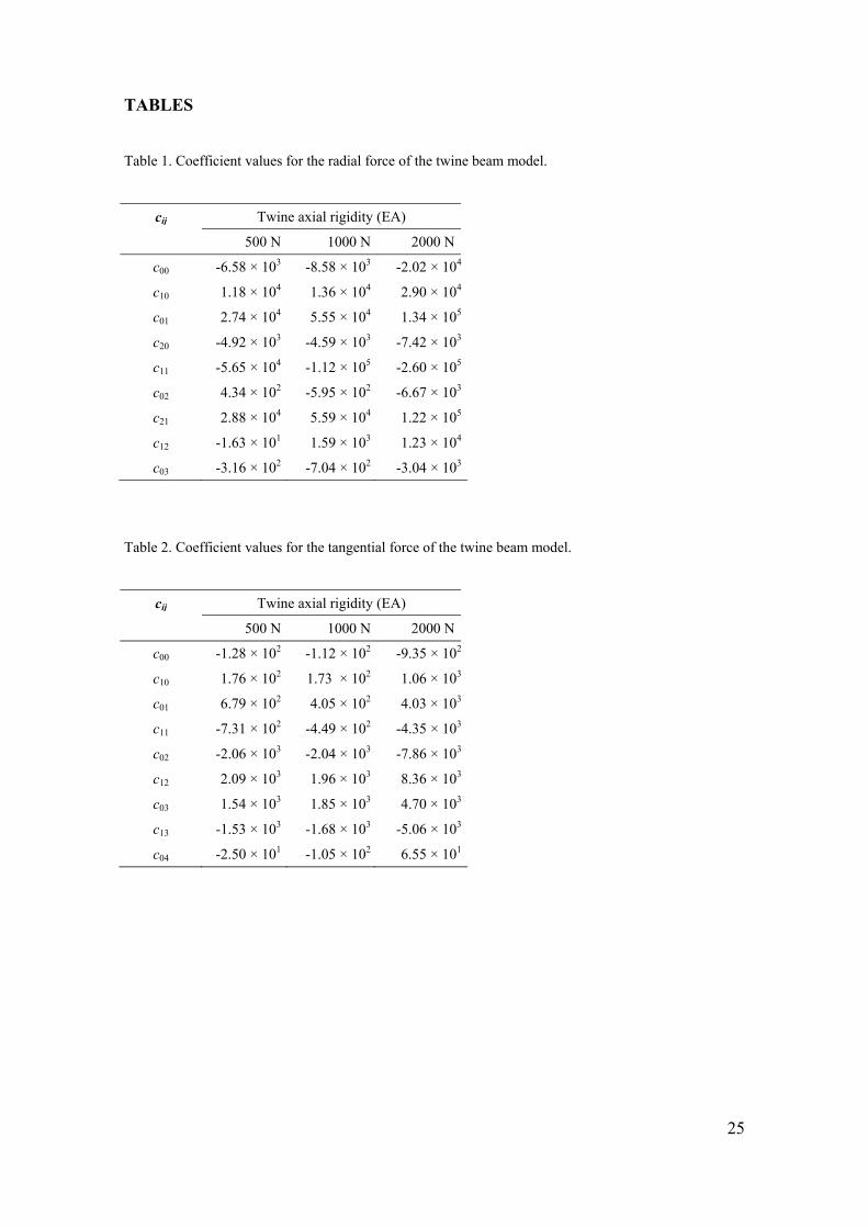
25
TABLES
Table 1. Coefficient values for the radial force of the twine beam model.
cij Twine axial rigidity (EA)
500 N 1000 N 2000 N
c00 -6.58 × 10³ -8.58 × 10³ -2.02 × 10⁴
c10 1.18 × 10⁴ 1.36 × 10⁴ 2.90 × 10⁴
c01 2.74 × 10⁴ 5.55 × 10⁴ 1.34 × 10⁵
c20 -4.92 × 10³ -4.59 × 10³ -7.42 × 10³
c11 -5.65 × 10⁴ -1.12 × 10⁵ -2.60 × 10⁵
c02 4.34 × 10² -5.95 × 10² -6.67 × 10³
c21 2.88 × 10⁴ 5.59 × 10⁴ 1.22 × 10⁵
c12 -1.63 × 101 1.59 × 10³ 1.23 × 10⁴
c03 -3.16 × 10² -7.04 × 10² -3.04 × 10³
Table 2. Coefficient values for the tangential force of the twine beam model.
cij Twine axial rigidity (EA)
500 N 1000 N 2000 N
c00 -1.28 × 10² -1.12 × 10² -9.35 × 10²
c10 1.76 × 10² 1.73 × 10² 1.06 × 10³
c01 6.79 × 10² 4.05 × 10² 4.03 × 10³
c11 -7.31 × 10² -4.49 × 10² -4.35 × 10³
c02 -2.06 × 10³ -2.04 × 10³ -7.86 × 10³
c12 2.09 × 10³ 1.96 × 10³ 8.36 × 10³
c03 1.54 × 10³ 1.85 × 10³ 4.70 × 10³
c13 -1.53 × 10³ -1.68 × 10³ -5.06 × 10³
c04 -2.50 × 101 -1.05 × 10² 6.55 × 101

26
Table 3. Computational performance of the presented model compared with a classical linear spring
model without mesh resistance to opening.
Presentedmodel
Classical linear spring model
Numerical meshes 10000 10000
Total solution time (s) 305.3 162.4
Force evaluation calls 10933 10804
Time per call (ms) 27.9 15.0
Time per call per mesh (s) 2.79 1.50
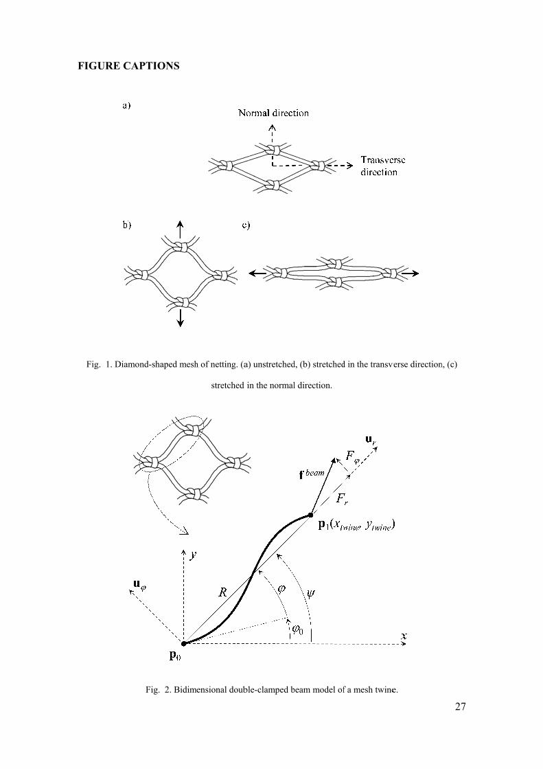
FIGU
Fig
URE CAPT
g. 1. Diamond
F
TIONS
d-shaped mesh
Fig. 2. Bidim
h of netting. (a
stretched
mensional doub
a) unstretched
in the normal
ble-clamped b
d, (b) stretched
l direction.
beam model of
d in the transv
f a mesh twine
verse direction
e.
27
n, (c)
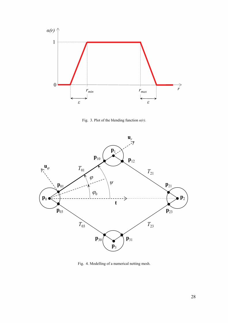
28
Fig. 3. Plot of the blending function α(r).
Fig. 4. Modelling of a numerical netting mesh.
ε
r
α(r)
1
ε
0rmin rmax
p2
p1
p0
p3
ur
u
p01
p03
p10 p12
p21
p23
p30 p31
T01 T21
T23T03
0
t
ψ
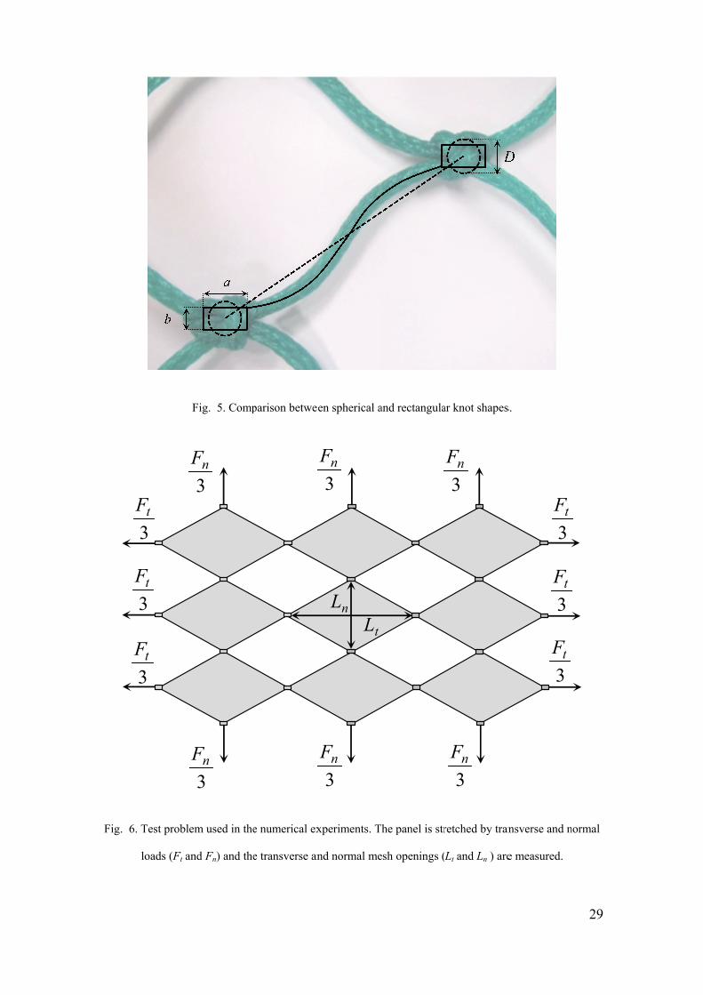
Fig. 6. Test proble
loads (Ft an
3tF
3tF
3tF
Fig. 5. Comp
em used in the
nd Fn) and the
3nF
3nF
parison betwe
e numerical ex
e transverse an
en spherical a
xperiments. T
nd normal me
Lt
Ln
3nF
3nF
and rectangula
The panel is str
esh openings (
ar knot shapes
retched by tran
Lt and Ln ) are
3nF
3nF
s.
nsverse and n
e measured.
3tF
3tF
3tF
29
normal
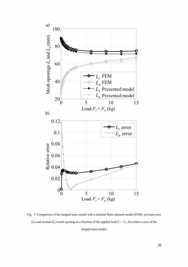
30
Fig. 7. Comparison of the lumped mass model with a detailed finite element model (FEM). (a) transverse
(Lt) and normal (Ln) mesh opening as a function of the applied load Ft = Fn, (b) relative error of the
lumped mass model.
0 5 10 1520
40
60
80
100
Lx FEMLy FEM Lx Presented modelLy Presented model
0 5 10 150
0.02
0.04
0.06
0.08
0.1
0.12
Error LxError Ly
Mes
h op
enin
gs L
tan
d L
n (m
m)
Lt
Ln
Lt
Ln
Load Ft = Fn (kg)
Load Ft = Fn (kg)
Rel
ativ
e er
ror
Lt errorLn error
a)
b)
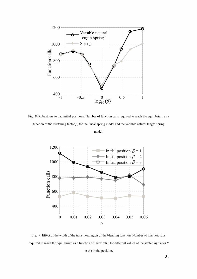
31
Fig. 8. Robustness to bad initial positions. Number of function calls required to reach the equilibrium as a
function of the stretching factor β, for the linear spring model and the variable natural length spring
model.
Fig. 9. Effect of the width of the transition region of the blending function. Number of function calls
required to reach the equilibrium as a function of the width ε for different values of the stretching factor β
in the initial position.
-1 -0.5 0 0.5 1400
600
800
1000
1200
Variable natural length springSpring
log10 (β)
Func
tion
calls
0 0.01 0.02 0.03 0.04 0.05 0.06
400
600
800
1000
1200
Initial position = 1Initial position = 2Initial position = 3
ε
βββ
Func
tion
calls
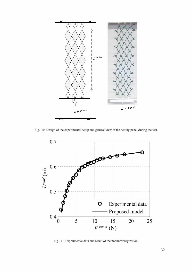
FFig. 10. Desi
Lpa
nel(m
)
0
0
0
0
gn of the expe
Fig. 11. Exp
00.4
0.5
0.6
0.7
erimental setu
perimental dat
5
up and general
ta and result o
panF
10
l view of the n
of the nonlinea
(N)nel15
ExperPropo
netting panel d
ar regression.
20
imental dosed mod
during the test
25
datadel
32
t.
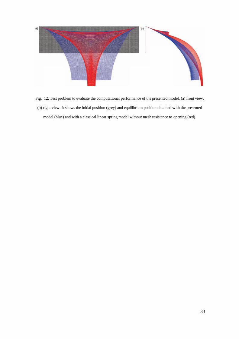
Fig.
(b) r
12. Test prob
right view. It
model (blue)
blem to evalua
shows the init
and with a cla
ate the comput
tial position (g
assical linear s
tational perfor
grey) and equ
spring model
rmance of the
uilibrium posit
without mesh
presented mo
tion obtained w
resistance to
odel. (a) front
with the prese
opening (red)
33
view,
ented
).