Embed Size (px)
Citation preview
Efficient Dilation, Erosion, Opening,and Closing Algorithms
Joseph (Yossi) Gil and Ron Kimmel, Senior Member, IEEE
Abstract—We propose an efficient and deterministic algorithm for computing the one-dimensional dilation and erosion (max and min)
sliding window filters. For a p-element sliding window, our algorithm computes the 1D filter using 1:5þ oð1Þ comparisons per sample
point. Our algorithm constitutes a deterministic improvement over the best previously known such algorithm, independently developed
by van Herk [25] and by Gil and Werman [12] (the HGW algorithm). Also, the results presented in this paper constitute an improvement
over the Gevorkian et al. [9] (GAA) variant of the HGW algorithm. The improvement over the GAA variant is also in the computation
model. The GAA algorithm makes the assumption that the input is independently and identically distributed (the i.i.d. assumption),
whereas our main result is deterministic. We also deal with the problem of computing the dilation and erosion filters simultaneously, as
required, e.g., for computing the unbiased morphological edge. In the case of i.i.d. inputs, we show that this simultaneous computation
can be done more efficiently then separately computing each. We then turn to the opening filter, defined as the application of the min
filter to the max filter and give an efficient algorithm for its computation. Specifically, this algorithm is only slightly slower than the
computation of just the max filter. The improved algorithms are readily generalized to two dimensions (for a rectangular window), as
well as to any higher finite dimension (for a hyperbox window), with the number of comparisons per window remaining constant. For the
sake of concreteness, we also make a few comments on implementation considerations in a contemporary programming language.
Index Terms—Mathematical morphology, running maximum filter, min-max filter, computational efficiency.
æ
1 INTRODUCTION
IN signal and image analysis, one often encounters theproblem of min (or max) computation in a window with
p elements in the one-dimensional (1D) case or p� p elementsin the two-dimensional (2D) case. In mathematical morphol-ogy [20], the result of such an operator is referred to as theerosion (or dilation) of the signal with a structuring elementgiven by a pulse of width p.
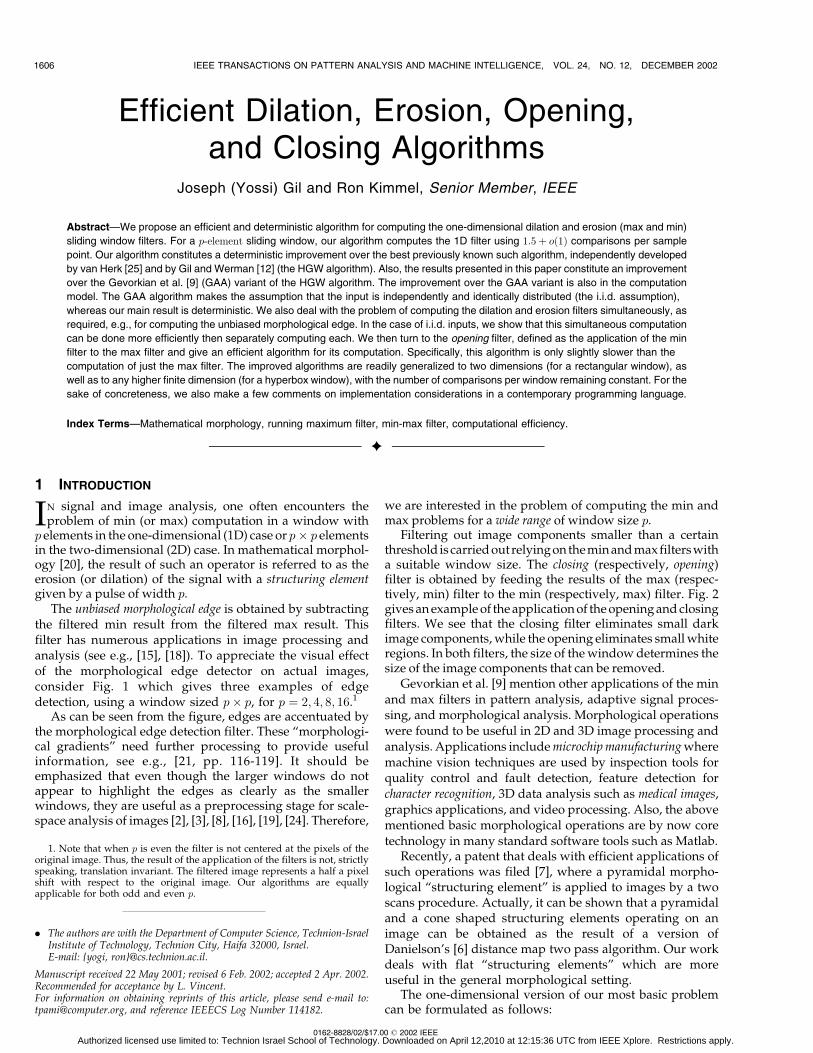
The unbiased morphological edge is obtained by subtractingthe filtered min result from the filtered max result. Thisfilter has numerous applications in image processing andanalysis (see e.g., [15], [18]). To appreciate the visual effectof the morphological edge detector on actual images,consider Fig. 1 which gives three examples of edgedetection, using a window sized p� p, for p ¼ 2; 4; 8; 16.1
As can be seen from the figure, edges are accentuated bythe morphological edge detection filter. These “morphologi-cal gradients” need further processing to provide usefulinformation, see e.g., [21, pp. 116-119]. It should beemphasized that even though the larger windows do notappear to highlight the edges as clearly as the smallerwindows, they are useful as a preprocessing stage for scale-space analysis of images [2], [3], [8], [16], [19], [24]. Therefore,
we are interested in the problem of computing the min andmax problems for a wide range of window size p.
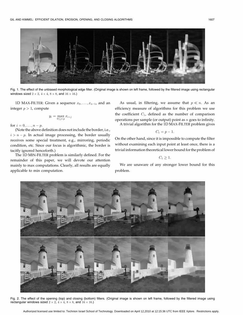
Filtering out image components smaller than a certainthreshold is carried out relying on themin and max filters witha suitable window size. The closing (respectively, opening)filter is obtained by feeding the results of the max (respec-tively, min) filter to the min (respectively, max) filter. Fig. 2gives an example of the application of the opening and closingfilters. We see that the closing filter eliminates small darkimage components, while the opening eliminates small whiteregions. In both filters, the size of the window determines thesize of the image components that can be removed.
Gevorkian et al. [9] mention other applications of the minand max filters in pattern analysis, adaptive signal proces-sing, and morphological analysis. Morphological operationswere found to be useful in 2D and 3D image processing andanalysis. Applications include microchip manufacturing wheremachine vision techniques are used by inspection tools forquality control and fault detection, feature detection forcharacter recognition, 3D data analysis such as medical images,graphics applications, and video processing. Also, the abovementioned basic morphological operations are by now coretechnology in many standard software tools such as Matlab.
Recently, a patent that deals with efficient applications ofsuch operations was filed [7], where a pyramidal morpho-logical “structuring element” is applied to images by a twoscans procedure. Actually, it can be shown that a pyramidaland a cone shaped structuring elements operating on animage can be obtained as the result of a version ofDanielson’s [6] distance map two pass algorithm. Our workdeals with flat “structuring elements” which are moreuseful in the general morphological setting.
The one-dimensional version of our most basic problemcan be formulated as follows:
1606 IEEE TRANSACTIONS ON PATTERN ANALYSIS AND MACHINE INTELLIGENCE, VOL. 24, NO. 12, DECEMBER 2002
. The authors are with the Department of Computer Science, Technion-IsraelInstitute of Technology, Technion City, Haifa 32000, Israel.E-mail: {yogi, ron}@cs.technion.ac.il.
Manuscript received 22 May 2001; revised 6 Feb. 2002; accepted 2 Apr. 2002.Recommended for acceptance by L. Vincent.For information on obtaining reprints of this article, please send e-mail to:[email protected], and reference IEEECS Log Number 114182.
1. Note that when p is even the filter is not centered at the pixels of theoriginal image. Thus, the result of the application of the filters is not, strictlyspeaking, translation invariant. The filtered image represents a half a pixelshift with respect to the original image. Our algorithms are equallyapplicable for both odd and even p.
0162-8828/02/$17.00 ß 2002 IEEEAuthorized licensed use limited to: Technion Israel School of Technology. Downloaded on April 12,2010 at 12:15:36 UTC from IEEE Xplore. Restrictions apply.
1D MAX-FILTER: Given a sequence x0; . . . ; xnÿ1, and an
integer p > 1, compute
yi ¼ max0�j<p
xiþj
for i ¼ 0; . . . ; nÿ p.(Note the above definition does not include the border, i.e.,
i > nÿ p. In actual image processing, the border usually
receives some special treatment, e.g., mirroring, periodic
condition, etc. Since our focus is algorithmic, the border is
tacitly ignored henceforth.)The 1D MIN-FILTER problem is similarly defined. For the
remainder of this paper, we will devote our attention
mainly to max computations. Clearly, all results are equally
applicable to min computation.
As usual, in filtering, we assume that p� n. As an
efficiency measure of algorithms for this problem we use
the coefficient C1, defined as the number of comparison
operations per sample (or output) point as n goes to infinity.A trivial algorithm for the 1D MAX-FILTER problem gives
C1 ¼ pÿ 1:
On the other hand, since it is impossible to compute the filter
without examining each input point at least once, there is a
trivial information theoretical lower bound for the problem of
C1 � 1:
We are unaware of any stronger lower bound for this
problem.
GIL AND KIMMEL: EFFICIENT DILATION, EROSION, OPENING, AND CLOSING ALGORITHMS 1607
Fig. 1. The effect of the unbiased morphological edge filter. (Original image is shown on left frame, followed by the filtered image using rectangular
windows sized 2� 2, 4� 4, 8� 8, and 16� 16.)
Fig. 2. The effect of the opening (top) and closing (bottom) filters. (Original image is shown on left frame, followed by the filtered image usingrectangular windows sized 2� 2, 4� 4, 8� 8, and 16� 16.)
Authorized licensed use limited to: Technion Israel School of Technology. Downloaded on April 12,2010 at 12:15:36 UTC from IEEE Xplore. Restrictions apply.
Pitas [17] describes two nontrivial algorithms for the
problem. The first such algorithm achieves C1 ¼ Oðlg pÞ.2Pitas’s second algorithm achieves C1 ¼ 3þ oð1Þ on the
average for i.i.d. input.3
Note that the worst case performance of both of thesealgorithms depends on the window size. In [25], van Herkandand, later, but independently, Gil and Werman [12] gave analgorithm (HGW) for computing the max filter whoseperformance does not depend on p. Gil and Werman’sdescription of the algorithm is slightly more general, showingthat the p sized filter of any semiring operation, �, can becomputed using 3ÿ 4=p applications of � per sample point.Since max is a semiring operation, we have that
C1 ¼ 3ÿ 4=p:
In the special case that the semiring operation is max andassuming i.i.d. input signal. Gevorkian et al. [9] gave analgorithm (GAA) that improves the HGW algorithm,achieving
EðC1Þ ¼ 2:5ÿ 3:5=p:
The expectation here is with respect to input distribution.We note that for many applications, such an assumption
is clearly invalid. In many natural signals, the probabilitythat xiþ > xi is greater than 0:5 if it is given that xi > xiÿ1. Inthe worst input case, such as an almost monotonicallyincreasing signal, the performance of the algorithm of GAAis the same as the HGW algorithm.
In this paper, we describe an algorithm achieving furtherreduction,
C1 ¼ 1:5þ lg p
pþOð1=pÞ:
This improvement is deterministic and does not make anyassumptions on the input distribution.
The morphological edge detector and other applicationsrequire the simultaneous computation of the min and max ineach window, as summarized in the following problemdefinition.
1D MAX-MIN-FILTER: Given a sequence x0; . . . ; xnÿ1, and
an integer p > 1, compute
yi ¼ max0�j<p
xiþj
zi ¼ min0�j<p
xiþj
for i ¼ 0; . . . ; nÿ p.We give an algorithm which solves 1D MAX-MIN-FILTER
problem faster than solving 1D MAX-FILTER and 1D MIN-
FILTER separately. Let Cm1 be the number of comparisons
per input sample for solving 1D MAX-MIN-FILTER. Then,
our algorithm achieves
EðCm1 Þ � 2þ 2:3466
lg p
p;
for the special case of independent input distribution, i.e., theexpectation is with regard to input distribution. In the worstcase, this algorithm does not improve on the independentcomputation of the Min and Max filters. However, for naturalimages, the algorithm makes such an improvement, althoughnot to the extent possible for randomized inputs.
The problem posed by the opening filter is similar to 1DMAX-MIN-FILTER since in both it is required to computeboth a Min-Filter and a Max-Filter. However, the fact that inthe opening filter this filters are computed sequentially,where the results of one filter are the input of the other,makes it much easier. Let Co
1 be the number of comparisonsper input sample for computing the opening filter. Then, weshow that
Co1 � C1 þO
lg2 p
p
� �:
Clearly, the same result holds for the closing filter.A 1D max filter can be extended to a rectangular window
2D max filter [12]. The extension is carried out by firstapplying the 1D filter along the rows and then feeding theresult to a 1D filter running along the columns. Let C2 be thenumber of comparison operations required per input pointfor computing the 2D max filter. We have that
C2 ¼ 2C1
and, more generally,
Cd ¼ dC1;
where Cd is defined accordingly for the d-dimensional filter.We similarly have that
Cmd ¼ dCm
1
Cod ¼ dCo
1 :
Outline. The remainder of this paper is organized asfollows: Section 2 reviews the HGW algorithm. Our mainresult which improves this algorithm is described in Section3. This section also makes a few comments on a randomizedversion of the algorithm and on an actual implementation ofthe algorithms in languages such as C [14]. In Section 4, wegive our algorithm for the 1D MAX-MIN FILTER problem.The efficient algorithm for computing the opening (andclosing) filter is described in Section 5. Finally, Section 6gives the conclusions and mentions a few open problems.
2 THE VAN HERK-GIL-WERMAN ALGORITHM
The van Herk-Gil-Werman (HGW) algorithm is based onsplitting the input signal to overlapping segments of size2pÿ 1, centered at
xpÿ1; x2pÿ1; x3pÿ1; . . . :
Let j be the index of an element at the center of a certainsegment. The maxima of the p windows which include xjare computed in one batch of the HGW algorithm as follows:First, define Rk and Sk for k ¼ 0; . . . ; pÿ 1:
Rk ¼ RkðjÞ ¼ maxðxj; xjÿ1; . . . ; xjÿkÞ;Sk ¼ SkðjÞ ¼ maxðxj; xjþ1; . . . ; xjþkÞ:
ð1Þ
1608 IEEE TRANSACTIONS ON PATTERN ANALYSIS AND MACHINE INTELLIGENCE, VOL. 24, NO. 12, DECEMBER 2002
2. We use lgð�Þ to denote log2ð�Þ.3. Here, and henceforth, we use the familiar oðfðpÞÞ notation for the
family of functions gðpÞ, such that limp!1gðpÞfðpÞ ¼ 0. Thus, oð1Þ are those
functions which tend to zero as p tends to infinity.
Authorized licensed use limited to: Technion Israel School of Technology. Downloaded on April 12,2010 at 12:15:36 UTC from IEEE Xplore. Restrictions apply.
Now, the Rks and the Sks can be merged together to
compute the max filter:
tk ¼ maxðxjÿk; . . . ; xj; . . . ; xjþpÿkÿ1Þ ¼ maxðRk; Spÿkÿ1Þ; ð2Þ
for k ¼ 1; . . . ; pÿ 2. In addition, we have
maxðxjÿpÿ1; . . . ; xjÞ ¼ Rpÿ1;
maxðx0; . . . ; xjþpÿ1Þ ¼ Spÿ1:
There are two stages to the HGW algorithm:
Preprocessing. Computing allRk andSk from their definition(1) and noting that Rk ¼ maxðRkÿ1; xjÿkÞ and Sk ¼maxðSkÿ1; xjþkÞ for k ¼ 1; . . . ; pÿ 1. This stage is carriedout in 2ðpÿ 1Þ comparisons.
Merge. Merging the Rk and Sk together using (2). This stagerequires another pÿ 2 comparisons. Since this procedurecomputes the maximum of p windows in total, we havethat the amortized number of comparisons per window is
2ðpÿ 1Þ þ pÿ 2
p¼ 3ÿ 4
p:
For large p, we have that the preprocessing step requirestwo comparison operations per element, while the mergestep requires one more such comparison.
3 THE IMPROVED ALGORITHMS FOR THE
MAX-FILTER
In this section, we show how the two steps of the
HGW algorithm can be carried out more efficiently.
3.1 An Efficient Preprocessing Computation
Let us now deal with the preprocessing step of theHGW algorithm. The observation behind the GAA algo-rithm is that preprocessing computation can be made moreefficient for randomized input, using the fact that in theHGW algorithm, the suffixes Sk of one segment overlapwith the prefixes Rk of the following segment. Specifically,the problem that needs to be solved is
PREFIX-SUFFIX MAX: Given a sequence x0; . . . ; xp, com-
pute all of its prefix maxima:
sk ¼ Skð0Þ ¼ maxðx0; . . . ; xkÞ;
for k ¼ 0; . . . ; pÿ 1, and all its suffix maxima:
rk ¼ RkðpÞ ¼ maxðxk; . . . ; xpÞ;
for k ¼ 1; . . . ; p.Note that this problem does not call for computing the
overall maximum of the input
sp ¼ r0 ¼ maxðx0; . . . ; xpÞ:
The original HGW algorithm makes 2ðpÿ 1Þ comparisonsin solving the PREFIX-SUFFIX MAX problem. We propose thefollowing efficient solution for this problem. Let
q ¼ pþ 1
2
� �¼ p
2þ p mod 2
2: ð3Þ
In the first part of the modified implementation, compute allsk, for k ¼ 0; . . . ; q ÿ 1, using q ÿ 1 comparisons and rk for
k ¼ q; . . . ; p, using pÿ q comparisons. The total number ofcomparisons in the first stage is then pÿ 1.
The second part of the modified implementation of thepreprocessing stage begins in comparing sqÿ1 and rq. Ifrq � sqÿ1, then we know that the overall maximum falls in oneof xq; . . . ; xp. Therefore, it is unnecessary to further computethe value of rqÿ1; rqÿ2; . . . ; r1. Instead, the algorithm outputs
rqÿ1 ¼ rqÿ2 ¼ . . . ¼ r1 ¼ rq;
and continues to compute sq; . . . ; spÿ1 in
pÿ q ¼ p2ÿ p mod 2
2ð4Þ
comparisons.A similar situation occurs if rq � sqÿ1, in which case it is
unnecessary to compute sq; . . . ; spÿ1. In this case, r1; . . . ; rqÿ1
are computed in
q ÿ 1 ¼ p2þ p mod 2
2ÿ 1 ð5Þ
comparisons.The number of comparisons in the second part is given
by the maximum of (4) and (5)
p
2ÿ p mod 2
2:
The total number of comparisons in the more efficientalgorithm for the preprocessing stage of PREFIX-SUFFIX
MAX is
ðpÿ 1Þ þ 1þ p2ÿ p bmod 2
2¼ 1:5pÿ p mod 2
2: ð6Þ
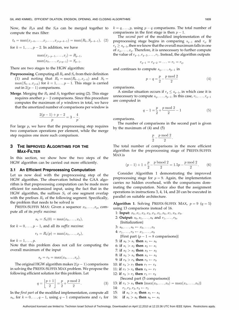
Consider Algorithm 1 demonstrating the improvedpreprocessing stage for p ¼ 9. Again, the implementationcarries no hidden overhead, with the comparisons dom-inating the computation. Notice also that the assignmentoperations in instructions 3, 4, 14, and 20 can be executed inparallel on suitable architecture.
Algorithm 1. Solving PREFIX-SUFFIX MAX, p ¼ 9 (q ¼ 5)using 13 comparisons instead of 16.
1: Input: x0; x1; x2; x3; x4; x5; x6; x7; x8; x9.
2: Output: s0; s1; . . . ; s8 and r1; . . . ; r9,
{Initialization}
3: s0; . . . ; s8 x0; . . . ; x8
4: r1; . . . ; r9 x1; . . . ; x9
{First part (pÿ 1 ¼ 8 comparisons)}
5: if s0 > s1 then s1 s0
6: if s1 > s2 then s2 s1
7: if s2 > s3 then s3 s2
8: if s3 > s4 then s4 s3
9: if r9 > r8 then r8 r9
10: if r8 > r7 then r7 r8
11: if r7 > r6 then r6 r7
12: if r6 > r5 then r5 r6
{Second part (5 comparisons)}13: if r5 > s4 then {maxðx0; . . . ; x9Þ ¼ maxðx5; . . . ; x9Þ}14: r1; r2; r3; r4 r5
15: if s4 > s5 then s5 s4
16: if s5 > s6 then s6 s5
GIL AND KIMMEL: EFFICIENT DILATION, EROSION, OPENING, AND CLOSING ALGORITHMS 1609
Authorized licensed use limited to: Technion Israel School of Technology. Downloaded on April 12,2010 at 12:15:36 UTC from IEEE Xplore. Restrictions apply.
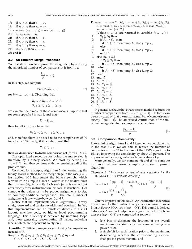
17: if s6 > s7 then s7 s6
18: if s7 > s8 then s8 s7
19: else {maxðx0; . . . ; x9Þ ¼ maxðx0; . . . ; x4Þ}20: s5; s6; s7; s8 s4
21: if r5 > r4 then r4 r5
22: if r4 > r3 then r3 r4
23: if r3 > r2 then r2 r3
24: ifr2 > r1 then r1 r2
25: end if
3.2 An Efficient Merge Procedure
We first show how to improve the merge step, by reducingthe amortized number of comparisons in it from 1 to
lg p
pþ oð1Þ:
In this step, we compute
maxðRk; Spÿkÿ1Þ; ð7Þ
for k ¼ 1; . . . ; pÿ 2. Observing that
Rpÿ2 � Rpÿ1 � . . . � R1;
Spÿ2 � Spÿ1 � . . . � S1;
we can eliminate most of these comparisons. Suppose thatfor some specific i it was found that
Ri � Spÿiÿ1;
then for all k > i, we have that
Rk � Ri � Spÿiÿ1 � Spÿkÿ1;
and, therefore, there is no need to do the comparisons of (7)for all k > i. Similarly, if it is determined that
Ri � Spÿiÿ1;
then we do not need to do the comparisons of (7) for all k < i.The optimized procedure for doing the merge step is
therefore by a binary search. We start by setting i ¼dðpÿ 2Þ=2e and then continue with the remaining half of theproblem size.
Consider, for example, Algorithm 2, demonstrating thebinary search method for the merge stage in the case p ¼ 9.Instruction 1-13 implement the binary search, whichterminates in a jump to a labelLi, where i is the smallest suchthat ti ¼ maxðRi; S8ÿiÞ ¼ Ri. Each such jump is carried outafter exactly three instructions in this case. Instructions 14-21compute the values of tis by proper assignments to Ris,without any additional comparisons. The total number ofassignments is any where between 0 and 7.
Notice that the implementation in Algorithm 2 is verystraightforward and carries no additional overhead. In fact,this implementation can be translated directly to a VLSIlayout, machine code, or higher level programminglanguage. This efficiency is achieved by unrolling loopsand, more generally, precomputing all values, includinglabels, which are dependent solely on p.
Algorithm 2. Efficient merge for p ¼ 9 using 3 comparisonsinstead of 7.Require: R1 � R2 � R3 � R4 � R5 � R6 � R7 and
S1 � S2 � S3 � S4 � S5 � S6 � S7
Ensure: t1 ¼ maxðR1; S7Þ, t2 ¼ maxðR2; S6Þ, t3 ¼ maxðR3; S5Þ,t4 ¼ maxðR4; S4Þ, t5 ¼ maxðR5; S3Þ, t6 ¼ maxðR6; S2Þ,and t7 ¼ maxðR7; S1Þ{Values t1; . . . ; t7 are returned in variables R1; . . . ; R7}
1: if R4 � S4 then2: if R2 � S6 then3: if R1 � S7 then jump L1 else jump L2
4: else5: if R3 � S5 then jump L3 else jump L4
6. end if7. else {R4 < S4}8. if R6 � S2 then9. if R5 � S3 then jump L5 else jump L6
10. else11. if R7 � S1 then jump L7 else jump L8
12. end if13. end if14. L8: R7 S1
15. L7: R6 S2
16. L6: R5 S3
17. L5: R4 S4
18. L4: R3 S5
19. L3: R2 S6
20. L2: R1 S7
21. L1:
In general, we have that binary search method reduces thenumber of comparisons frompÿ 2 to lg pþOð1Þ. In fact, it canbe easily checked that the maximal number of comparisons isexactly dlgðpÿ 1Þe. The amortized contribution of the im-proved merge step to the complexity is therefore
dlgðpÿ 1Þep
: ð8Þ
3.3 Comparison Complexity
In examining Algorithms 1 and 2 together, we conclude thatin the case p ¼ 9, we are able to reduce the number ofcomparisons from 23 in the case of the HGW algorithm to16, i.e., improving the complexity by about 30 percent. Theimprovement is even greater for larger values of p.
More generally, we can combine (6) and (8) to computethe amortized comparison complexity of our improvedalgorithm.
Theorem 1. There exists a deterministic algorithm for the1D MAX-FILTER problem, achieving
C1 ¼ 1:5þ dlgðpÿ 1Þep
ÿ p mod 2
2p� 1:5þ dlgðpÿ 1Þe
p
¼ 1:5þ lg p
pþO 1
p
� �:
ð9Þ
Can we improve on this result? An information theoreticallower bound for the number of comparisons required to solvePREFIX-SUFFIX MAX, is pþ lg pÿOð1Þ. This bound is derivedas follows: A compact output of an algorithm for the problemuses pþ lg pÿOð1Þ bits comprised as follows:
1. lg p bits to designate the location of the overallmaximum (for simplicity, we assume that p is apower of 2),
2. a single bit for each location prior to the maximum,designating whether the corresponding elementchanges the prefix maxima, and
1610 IEEE TRANSACTIONS ON PATTERN ANALYSIS AND MACHINE INTELLIGENCE, VOL. 24, NO. 12, DECEMBER 2002
Authorized licensed use limited to: Technion Israel School of Technology. Downloaded on April 12,2010 at 12:15:36 UTC from IEEE Xplore. Restrictions apply.
3. a single bit for each location following to themaximum, designating whether the correspondingelement changes the suffix maxima.
Moreover, there are distinct inputs which produce all the bit
combinations of this compact representation. Thus, in order
to make the distinction between these inputs, the algorithm
is forced to make at least
pþ lg pÿOð1Þ ð10Þ
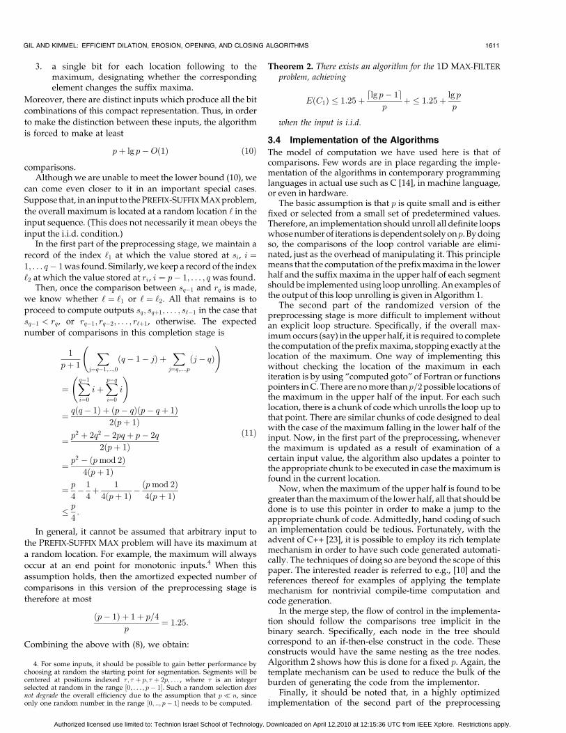
comparisons.Although we are unable to meet the lower bound (10), we
can come even closer to it in an important special cases.
Suppose that, in an input to the PREFIX-SUFFIX MAX problem,
the overall maximum is located at a random location ‘ in the
input sequence. (This does not necessarily it mean obeys the
input the i.i.d. condition.)In the first part of the preprocessing stage, we maintain a
record of the index ‘1 at which the value stored at si, i ¼1; . . . q ÿ 1 was found. Similarly, we keep a record of the index
‘2 at which the value stored at ri, i ¼ pÿ 1; . . . ; q was found.Then, once the comparison between sqÿ1 and rq is made,
we know whether ‘ ¼ ‘1 or ‘ ¼ ‘2. All that remains is to
proceed to compute outputs sq; sqþ1; . . . ; s‘ÿ1 in the case that
sqÿ1 < rq, or rqÿ1; rqÿ2; . . . ; r‘þ1, otherwise. The expected
number of comparisons in this completion stage is
1
pþ 1
Xj¼qÿ1;...;0
ðq ÿ 1ÿ jÞ þX
j¼q;...;pðjÿ qÞ
!
¼Xqÿ1
i¼0
iþXpÿqi¼0
i
!
¼ qðq ÿ 1Þ þ ðpÿ qÞðpÿ q þ 1Þ2ðpþ 1Þ
¼ p2 þ 2q2 ÿ 2pq þ pÿ 2q
2ðpþ 1Þ
¼ p2 ÿ ðpmod 2Þ
4ðpþ 1Þ
¼ p4ÿ 1
4þ 1
4ðpþ 1Þ ÿðpmod 2Þ4ðpþ 1Þ
� p4:
ð11Þ
In general, it cannot be assumed that arbitrary input to
the PREFIX-SUFFIX MAX problem will have its maximum at
a random location. For example, the maximum will always
occur at an end point for monotonic inputs.4 When this
assumption holds, then the amortized expected number of
comparisons in this version of the preprocessing stage is
therefore at most
ðpÿ 1Þ þ 1þ p=4
p¼ 1:25:
Combining the above with (8), we obtain:
Theorem 2. There exists an algorithm for the 1D MAX-FILTER
problem, achieving
EðC1Þ � 1:25þ dlg pÿ 1ep
þ � 1:25þ lg p
p
when the input is i.i.d.
3.4 Implementation of the Algorithms
The model of computation we have used here is that ofcomparisons. Few words are in place regarding the imple-mentation of the algorithms in contemporary programminglanguages in actual use such as C [14], in machine language,or even in hardware.
The basic assumption is that p is quite small and is eitherfixed or selected from a small set of predetermined values.Therefore, an implementation should unroll all definite loopswhose number of iterations is dependent solely onp. By doingso, the comparisons of the loop control variable are elimi-nated, just as the overhead of manipulating it. This principlemeans that the computation of the prefix maxima in the lowerhalf and the suffix maxima in the upper half of each segmentshould be implemented using loop unrolling. An examples ofthe output of this loop unrolling is given in Algorithm 1.
The second part of the randomized version of thepreprocessing stage is more difficult to implement withoutan explicit loop structure. Specifically, if the overall max-imum occurs (say) in the upper half, it is required to completethe computation of the prefix maxima, stopping exactly at thelocation of the maximum. One way of implementing thiswithout checking the location of the maximum in eachiteration is by using “computed goto” of Fortran or functionspointers in C. There are no more than p=2 possible locations ofthe maximum in the upper half of the input. For each suchlocation, there is a chunk of code which unrolls the loop up tothat point. There are similar chunks of code designed to dealwith the case of the maximum falling in the lower half of theinput. Now, in the first part of the preprocessing, wheneverthe maximum is updated as a result of examination of acertain input value, the algorithm also updates a pointer tothe appropriate chunk to be executed in case the maximum isfound in the current location.
Now, when the maximum of the upper half is found to begreater than the maximum of the lower half, all that should bedone is to use this pointer in order to make a jump to theappropriate chunk of code. Admittedly, hand coding of suchan implementation could be tedious. Fortunately, with theadvent of C++ [23], it is possible to employ its rich templatemechanism in order to have such code generated automati-cally. The techniques of doing so are beyond the scope of thispaper. The interested reader is referred to e.g., [10] and thereferences thereof for examples of applying the templatemechanism for nontrivial compile-time computation andcode generation.
In the merge step, the flow of control in the implementa-tion should follow the comparisons tree implicit in thebinary search. Specifically, each node in the tree shouldcorrespond to an if-then-else construct in the code. Theseconstructs would have the same nesting as the tree nodes.Algorithm 2 shows how this is done for a fixed p. Again, thetemplate mechanism can be used to reduce the bulk of theburden of generating the code from the implementor.
Finally, it should be noted that, in a highly optimizedimplementation of the second part of the preprocessing
GIL AND KIMMEL: EFFICIENT DILATION, EROSION, OPENING, AND CLOSING ALGORITHMS 1611
4. For some inputs, it should be possible to gain better performance bychoosing at random the starting point for segmentation. Segments will becentered at positions indexed �; � þ p; � þ 2p; . . . , where � is an integerselected at random in the range ½0; . . . ; pÿ 1�. Such a random selection doesnot degrade the overall efficiency due to the assumption that p� n, sinceonly one random number in the range ½0; ::; pÿ 1� needs to be computed.
Authorized licensed use limited to: Technion Israel School of Technology. Downloaded on April 12,2010 at 12:15:36 UTC from IEEE Xplore. Restrictions apply.
stage, if the overall maximum is found in the lower half, allprefix maxima of the upper half are equal to this overallmaximum, and there is no need to actually produce or storethem in an auxiliary array. Instead, these values could beinlined into the code of the merge step.
4 EFFICIENT ALGORITHM FOR SIMULTANEOUSLY
COMPUTING THE MAX- AND MIN-FILTERS
In this section, we deal with the 1D MAX-MIN FILTER
problem and show how computing the min and max filterssimultaneously can be done more efficiently than anindependent computation of both. We start again with theHGW algorithm. The gain comes from partitioning the inputsignal into pairs of consecutive elements, and comparing thevalues in each pair. The greater value in each pair carries onthe maximum computation while the lesser one carries one tothe minimum computation.
4.1 The Prefix Max-Min Problem
Let us first consider the following problem:PREFIX MAX-MIN: Given a sequence x0; . . . ; xqÿ1, compute
Mk ¼ maxðx0; . . . ; xkÞ;mk ¼ minðx0; . . . ; xkÞ;
for k ¼ 0; . . . ; q ÿ 1.The straightforward solution for PREFIX MAX-MIN uses atotal of 2ðq ÿ 2Þ þ 1 comparisons. For the sake of simplicity,we assume that all elements in the input sequence are distinct.Analyzing this problem from an information theoretical pointof view, the algorithm is tantamount to classifying eachelement xi, i > 2, into one of three categories. Element xi mayincrease the running prefix maximum, i.e., xi > Mkÿ1 and,therefore,Mk ¼ xi. If this is not the case, then xi may decreasethe running minimum, i.e., xi < mkÿ1. The third case is thatmkÿ1 � xi < Mkÿ1 and, therefore, no changes are made to bemade to the running prefix minimum or maximum. Also,there are only two possible cases for x1, while there is exactlyone case for x0. Thus, we obtain
1þ ðq ÿ 2Þ lg 3 � 1:58496q;
as an information theoretic lower bound for the number ofcomparisons for the PREFIX MAX-MIN problem.
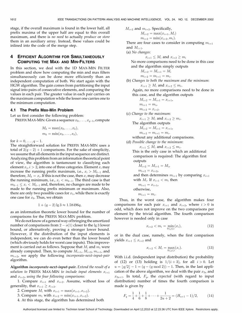
We do not know of a general way of bringing the amortizednumber of comparisons from 2ÿ oð1Þ closer to the lg 3 lowerbound, or alternatively, proving a stronger lower bound.However, if the distribution of the input elements isindependent, we can do even better than the lower bound(which obviously holds for worst case inputs). This improve-ment is carried out as follows. Suppose that Mi and mi werealready computed. Then, to compute Miþ1, Miþ2, miþ1, andmiþ2, we apply the following incorporate-next-input-pairalgorithm.
Algorithm incorporate-next-input-pair. Extend the result of a
solution to PREFIX MAX-MIN to include input elements xiþ1
and xiþ2, using the four following comparisons:
1. Compare xiþ1 and xiþ2. Assume, without loss of
generality, that xiþ1 � xiþ2.
2. Compare Mi with xiþ1 ¼ maxðxiþ1; xiþ2Þ.3. Compare mi with xiþ2 ¼ minðxiþ1; xiþ2Þ.4. At this stage, the algorithm has determined both
Miþ2 and miþ2. Specifically,Miþ2 ¼ maxðxiþ1;MiÞmiþ2 ¼ minðxiþ2;miÞ.
There are four cases to consider in computing miþ1
and Miþ1.
(a) No changes:
xiþ1 �Mi and xiþ2 � mi
No more comparisons need to be done in this case
and the algorithm simply outputsMiþ2 ¼Miþ1 ¼Mi
miþ2 ¼ miþ1 ¼ mi.
(b) Changes to both the maximum and the minimum:
xiþ1 �Mi and xiþ2 � mi.
Again, no more comparisons need to be done in
this case, and the algorithm outputs
Miþ2 ¼Miþ1 ¼ xiþ1,
miþ1 ¼ mi,miþ2 ¼ xiþ2.
(c) Change to the maximum:
xiþ1 �Mi and xiþ2 � mi.
The algorithm outputs
Miþ2 ¼Miþ1 ¼ xiþ1,
miþ2 ¼ miþ1 ¼ mi.
without any additional comparisons.
(d) Possible change to the minimum:xiþ1 �Mi and xiþ2 � mi.
This is the only case in which an additional
comparison is required: The algorithm first
outputs
Miþ2 ¼Miþ1 ¼Mi,
miþ2 ¼ xiþ2,
and then determines miþ1 by comparing xiþ1
with Mi. If xiþ1 < mi thenmiþ1 ¼ xiþ1,
otherwise,
miþ1 ¼ mi.
Thus, in the worst case, the algorithm makes fourcomparisons for each pair xiþ1 and xiþ2, where i > 0 isodd, which does not improve on the two comparisons perelement by the trivial algorithm. The fourth comparisonhowever is needed only in case
xiþ2 < mi ¼ min0�j�iðxiÞ; ð12Þ
or in the dual case, namely, when the first comparison
yields xiþ1 � xiþ2 and
xiþ2 < Mi ¼ max0�j�iðxiÞ: ð13Þ
With i.i.d. (independent input distribution) the probability
of (12) or (13) holding is 1=ðiþ 3Þ, for all i > 0. Let
u ¼ bq=2c ÿ 1 ¼ ðq ÿ ðq mod 2ÞÞ ÿ 1. Then, in the last appli-
cation of the above algorithm, we deal with the pair x2u and
x2uþ1. In total, Fq, the expected (with regard to input
distribution) number of times the fourth comparison is
made is given by
Fq ¼1
4þ 1
6þ 1
8þ � � � þ 1
2uþ 2¼ ðHuþ1 ÿ 1Þ=2; ð14Þ
1612 IEEE TRANSACTIONS ON PATTERN ANALYSIS AND MACHINE INTELLIGENCE, VOL. 24, NO. 12, DECEMBER 2002
Authorized licensed use limited to: Technion Israel School of Technology. Downloaded on April 12,2010 at 12:15:36 UTC from IEEE Xplore. Restrictions apply.
where Hu is the uth harmonic number. It is well known that
limu!1
Hu ¼ lnuþ ; ð15Þ
where � 0:577216 is Euler’s constant (also called Mascher-oni’s constant). Combining (14) and (15), we have
Fq ¼lnðuþ 1Þ
2þ
2ÿ 0:5þ oð1Þ
� lnðuþ 1Þ2
ÿ 0:211392þ oð1Þ:ð16Þ
It is also known that
lnuþ � Hu � lnuþ 1 ð17Þ
from which we obtain
Fq �lnðuþ 1Þ
2
� ln q ÿ 1
2:
ð18Þ
Other than these, in solving PREFIX MAX-MIN, there areu applications of incorporate-next-input-pair, in which 3ucomparisons are made, one comparison in which x0 iscompared with x1 to determine M0, M1, m0, and m1, andfinally, and only if q is odd, two comparisons to determineMqÿ1 and mqÿ1. The number of these comparisons is
1þ 3uþ 2ðq mod 2Þ ¼ 3q
2ÿ 2þ q mod 2
2: ð19Þ
Adding (18) and (19), we have that the expected totalnumber of comparisons in our solution to PREFIX MAX-MIN
is at most
3q
2þ ln q
2ÿ 2 ð20Þ
and the expected amortized number of comparisons perelement is at most
1:5þ ln q
2qÿ 2=q:
It should be noted that one cannot hope to improve much onthis result. The reason is that solving PREFIX MAX-MIN alsoyields the maximum and the minimum of the whole input.However, computing both these values cannot be done in lessthan d3p=2e comparisons [5, p. 187] even for randomizedinputs.
4.2 Computing the Min-Max Filter
We now employ algorithm incorporate-next-input-pair in thepreprocessing stage of the modified HGW algorithmadapted for finding both the minimum and the maximumfilters. Specifically, we are concerned in this stage in findingan efficient algorithm to the PREFIX-SUFFIX MAX-MIN
problem, defined as computing the maximum and theminimum of all prefixes and all suffixes of an array of sizepþ 1. Such an efficient algorithm is obtained by partitioningthe input array into two halves. In the lower half, whichcomprises q ¼ bðpþ 1Þ=2c ¼ p=2þ ðpmod 2Þ=2 elements, werepetitively apply incorporate-next-input-pair to compute theprefix maxima and the prefix minima in this half. A similarcomputation is carried out in the upper half with pÿ q þ1 ¼ dðpþ 1Þ=2e elements of the input array, except that
algorithm incorporate-next-input-pair is mirrored to computethe suffix minima and the suffix maxima in this half. Thetotal expected number of comparisons so far can becomputed from (20):
3q
2þ 3ðpþ 1ÿ qÞ
2þ ln q
2þ lnðpþ 1ÿ qÞ
2ÿ 4
¼ 3p
2þ lnðbðpþ 1Þ=2cdðpþ 1Þ=2e
2ÿ 2:5
� 3p
2þ
ln pþ12
ÿ �2
2ÿ 2:5
¼ 3p
2þ lnðpþ 1Þ ÿ ln 2ÿ 2:5
� 3p
2þ ln pÿ 2:5:
ð21Þ
Once this computation is done, we carry on as before toproduce the rest of the required output. In two morecomparisons, we find out where the maximum and theminimum of the whole array occur. If the maximum occursin the lower (respectively, upper) half then, it remains tocompute the suffix (respectively, prefix) maxima from themid-point down-to (respectively, up-to) the location of themaximum. From (11), we have that this computation costsanother 0.25 comparison per input element. A similarcompletion stage must be carried out for the minimumprefixes or suffixes, using another 0.25 amortized compar-isons. All that remains to do is the merge step which has tobe carried out twice, once for the minimum and once for themaximum. The number of comparisons for the merge is atmost 2 lg p. Combining this bound with (21) we obtain:
Theorem 3. There exists an algorithm for the 1D MIN-MAX
FILTER problem that, at the worst case, makes twice the number
of comparisons as that of Theorem 2. For i.i.d. input, the
amortized number of comparisons that the algorithm makes is
Cm1 < 2þ 2
ln pþ lg p
p
¼ 2þ 2þ ln 2
2
� �lg p
p
� 2þ 2:3466lg p
p:
Stated differently, we have that asymptotically for largep, and for i.i.d. one comparison per element is required tocompute each of the minimum and the maximum filters,provided they are computed together.
4.3 Performance on Natural Images
Natural images are far from being random inputs. It istherefore important to check the performance of thealgorithm of Theorem 3 in natural images. The importantfactor isKp, the number of times the prefix maximum (or theprefix minimum) is changed in a window of size p. Clearly,1 � Kp � p. With randomized input, the expected value ofKp
is Hp � ln pþ , which gives rise to an asymptotic saving of0:5 comparison per input value. If, on the other hand, theinput is monotonically increasing thenKp ¼ p. This is a worstcase input in which no savings at all can be made incomputing the min and max filters together. More generally,the amortized number of comparisons that are saved by the
GIL AND KIMMEL: EFFICIENT DILATION, EROSION, OPENING, AND CLOSING ALGORITHMS 1613
Authorized licensed use limited to: Technion Israel School of Technology. Downloaded on April 12,2010 at 12:15:36 UTC from IEEE Xplore. Restrictions apply.
iterative application of incorporate-next-input-pair is in theorder of
pÿKp
p:
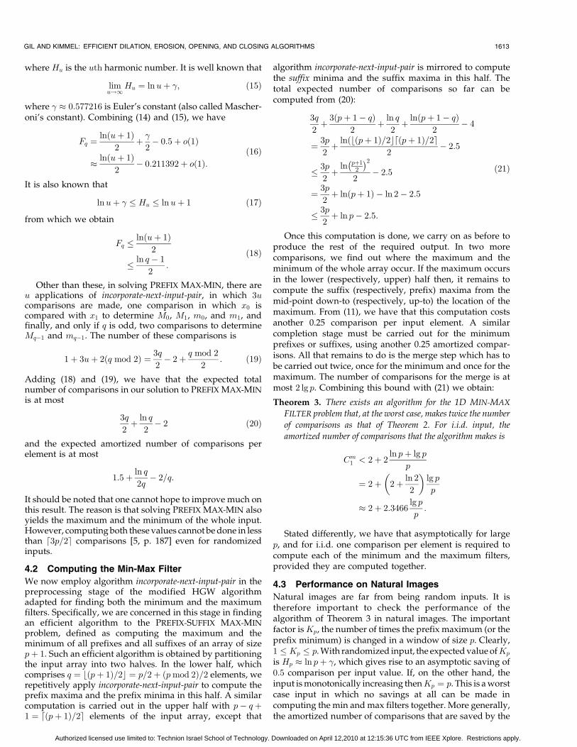
Fig. 3 shows the average value of Kp (using maxcomputation) for p ¼ 2; . . . ; 100 in the lighthouse image. Inthis, and all subsequent figures, the average was computed byexamining all one-dimensional row windows in the image.Only windows which entirely fall in the image wereconsidered. For comparison purposes, this figure, just as allthe ones to follow, shows the rate at whichHp increases withp.
Fig. 3a shows the average value of Kp for the red, green,and blue components of each pixel. It is interesting to notethat these three channels behave quite similarly and as weshall see next, very much like the behavior of theillumination in gray-level images. For small values of p,Kp, and Hp are close and Kp appears to increase in alogarithmic rate. For larger values of p, Kp appears toincrease at a linear rate, with
9 � K100 � 12:
It is also interesting to note that the rate of increase ofKp is thefastest in the red channel and slowest in the blue channel.
Fig. 3b is similar to Fig. 3a except that it depicts the rateof increase of Kp for minimum computation.
We witness again the same phenomena: The rate ofincrease inKp is faster than that ofHp, it is slowest to changein the blue and fastest in the red. Curiously, we have a slightlybetter ratio for Kp=p for the minimum computation
8 � K100 � 10:
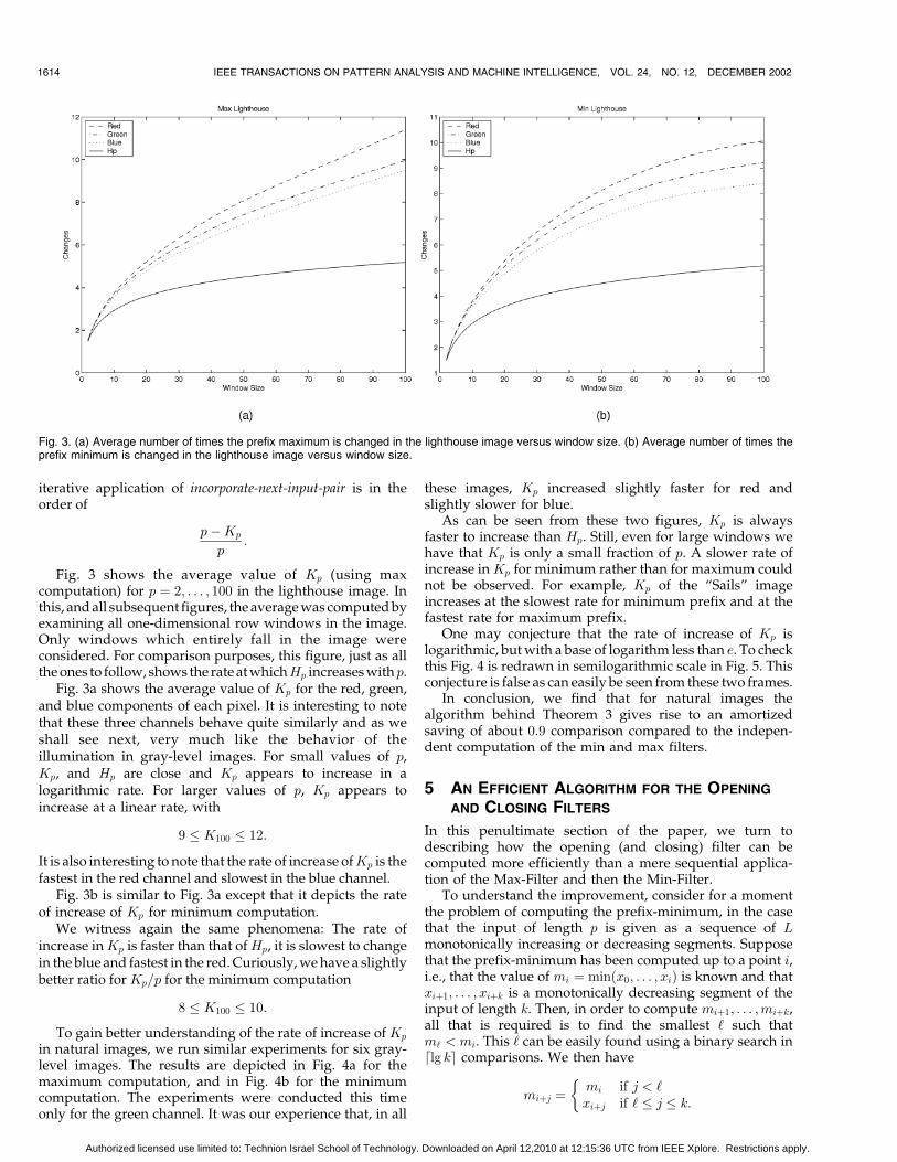
To gain better understanding of the rate of increase of Kp
in natural images, we run similar experiments for six gray-level images. The results are depicted in Fig. 4a for themaximum computation, and in Fig. 4b for the minimumcomputation. The experiments were conducted this timeonly for the green channel. It was our experience that, in all
these images, Kp increased slightly faster for red andslightly slower for blue.
As can be seen from these two figures, Kp is alwaysfaster to increase than Hp. Still, even for large windows wehave that Kp is only a small fraction of p. A slower rate ofincrease in Kp for minimum rather than for maximum couldnot be observed. For example, Kp of the “Sails” imageincreases at the slowest rate for minimum prefix and at thefastest rate for maximum prefix.
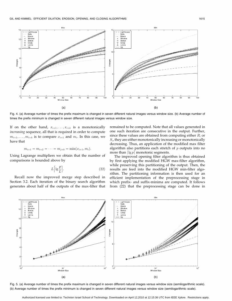
One may conjecture that the rate of increase of Kp islogarithmic, but with a base of logarithm less than e. To checkthis Fig. 4 is redrawn in semilogarithmic scale in Fig. 5. Thisconjecture is false as can easily be seen from these two frames.
In conclusion, we find that for natural images thealgorithm behind Theorem 3 gives rise to an amortizedsaving of about 0:9 comparison compared to the indepen-dent computation of the min and max filters.
5 AN EFFICIENT ALGORITHM FOR THE OPENING
AND CLOSING FILTERS
In this penultimate section of the paper, we turn todescribing how the opening (and closing) filter can becomputed more efficiently than a mere sequential applica-tion of the Max-Filter and then the Min-Filter.
To understand the improvement, consider for a momentthe problem of computing the prefix-minimum, in the casethat the input of length p is given as a sequence of Lmonotonically increasing or decreasing segments. Supposethat the prefix-minimum has been computed up to a point i,i.e., that the value of mi ¼ minðx0; . . . ; xiÞ is known and thatxiþ1; . . . ; xiþk is a monotonically decreasing segment of theinput of length k. Then, in order to compute miþ1; . . . ;miþk,all that is required is to find the smallest ‘ such thatm‘ < mi. This ‘ can be easily found using a binary search indlg ke comparisons. We then have
miþj ¼mi if j < ‘xiþj if ‘ � j � k:
�
1614 IEEE TRANSACTIONS ON PATTERN ANALYSIS AND MACHINE INTELLIGENCE, VOL. 24, NO. 12, DECEMBER 2002
Fig. 3. (a) Average number of times the prefix maximum is changed in the lighthouse image versus window size. (b) Average number of times theprefix minimum is changed in the lighthouse image versus window size.
Authorized licensed use limited to: Technion Israel School of Technology. Downloaded on April 12,2010 at 12:15:36 UTC from IEEE Xplore. Restrictions apply.
If on the other hand, xiþ1; . . . ; xiþk is a monotonically
increasing sequence, all that is required in order to compute
miþ1; . . . ;miþk is to compare xiþ1 and mi. In this case, we
have that
miþ1 ¼ miþ2 ¼ � � � ¼ mjþk ¼ minðxiþ1; miÞ:
Using Lagrange multipliers we obtain that the number of
comparisons is bounded above by
L lgp
L
l m: ð22Þ
Recall now the improved merge step described in
Section 3.2. Each iteration of the binary search algorithm
generates about half of the outputs of the max-filter that
remained to be computed. Note that all values generated inone such iteration are consecutive in the output. Further,since these values are obtained from computing either Ri orSi, they are either monotonically increasing or monotonicallydecreasing. Thus, an application of the modified max filteralgorithm also partitions each stretch of p outputs into nomore than dlg pemonotonic segments.
The improved opening filter algorithm is thus obtainedby first applying the modified HGW max-filter algorithm,while preserving this partitioning of the output. Then, theresults are feed into the modified HGW min-filter algo-rithm. The partitioning information is then used for anefficient implementation of the preprocessing stage inwhich prefix- and suffix-minima are computed. It followsfrom (22) that the preprocessing stage can be done in
GIL AND KIMMEL: EFFICIENT DILATION, EROSION, OPENING, AND CLOSING ALGORITHMS 1615
Fig. 4. (a) Average number of times the prefix maximum is changed in seven different natural images versus window size. (b) Average number of
times the prefix minimum is changed in seven different natural images versus window size.
Fig. 5. (a) Average number of times the prefix maximum is changed in seven different natural images versus window size (semilogarithmic scale).
(b) Average number of times the prefix minimum is changed in seven different natural images versus window size (semilogarithmic scale).
Authorized licensed use limited to: Technion Israel School of Technology. Downloaded on April 12,2010 at 12:15:36 UTC from IEEE Xplore. Restrictions apply.
Oðlg2 pÞ comparisons. Since the merge step can be done inOðlg pÞ comparisons, we obtain:
Theorem 4. There exists an algorithm which computes theopening filter, achieving
Co1 ¼ C1 þO
lg2 p
p
� �:
In other words, asymptotically computing the openingfilter is not more expensive than computing just the max-filter. When going to more than one dimension, unlike theerosion and dilation, the opening and closing operations arenot separable and, thus, do not enjoy the same computa-tional efficiency as the one-dimensional opening and andclosing. Nevertheless, one could still use the one-dimen-sional efficiency to accelerate these operations. The order ofoperations in this case could be the following:
. Apply the MAX FILTER on the rows. For non-i.i.d.signals, this operation takes C1 comparisons.
. Apply the MIN-MAX FILTER on the columns of theresult of the previous step. For non-i.i.d. signals, thisoperation takes C1 þ oð1Þ comparisons.
. Apply the MIN FILTER on the rows of the result ofthe the previous step. For non-i.i.d., it takes C1
comparisons.
That is, for two-dimensional images, instead of using 4C1 ¼6 comparisons per element, we spend only 3C1 ¼ 4:5comparisons per element (or 3:75 comparisons instead of 5for i.i.d. signals). For the general n-dimensional case, wespend ðnÿ 1ÞC1 comparisons, exploiting the fact that atleast for one dimension we can enjoy the efficiency of the1D MIN-MAX FILTER.
6 CONCLUSIONS AND OPEN PROBLEMS
We presented improvements of the HGW algorithm forrunning min and max filters. The average computationalcomplexity was shown to be 1:25þ oð1Þ per element forrandomized input, and 1:5þ oð1Þ for a deterministic algo-rithm (worst case input). These improvements, which comeclose to the best-known lower bound for the problem, wereenabled by careful examination of the redundancies in thepreprocessing and the merge steps of the HGW algorithm.
We continued to study a related problem, namely thecomputation of the min and the max filter together. We foundthat for i.i.d. input, it is possible to compute the minimum andthe maximum filters together in 2þ oð1Þ comparisons perdata point. This is less than 2:5þ oð1Þ comparisons requiredby applying twice the best max filter algorithm.
The opening and closing filters which are similar to theproblem of computing the min- and max-filters together, canbe computed much more efficiently. We found algorithms forthese filters using 1:5þ oð1Þ comparisons deterministically,or 1:25þ oð1Þ comparisons when the input is i.i.d.
All separable algorithms like erosion and dilation arereadily extendible to higher dimensions.
We leave the following open questions for furtherresearch:
1. In image processing, the selection of a coordinatesystem is usually arbitrary and unrelated to the
geometry of the objects being presented. Therefore, itseems more natural to use a circle rather than asquare as the shape of the window. However, theextension of the 1D algorithm for a 2D circle caseneeds further thought. By using a heap datastructure to represent a sliding window in the shapeof a circle of radius p, we can compute the filter in
Oðp lg pÞ
comparisons per window; in each move of the centerof the circle, the data structure is updated by addingOðpÞ points and removing OðpÞ points. If pixel valuesare drawn from some small finite domain, then it ispossible to use a dynamic moving histogram [13], [4]data structure supporting insertions and deletions inOð1Þ time. The amortized cost is then reduced toOðpÞ.It is interesting and important to find more efficientaccurate algorithms for this problem, with and withoutassuming that pixel values are bounded. (Previousresults [1], [22] give approximations to this problem.)
2. We know of no deterministic or randomized algo-rithm which computes for worst case input the MAX-
MIN FILTER more efficiently than computing themin and max separately. However, there is aninteresting property of algorithm incorporate-next-input-pair which might be used in trying to meet thischallenge: The fourth comparison is only requiredfor the computation of the interim Miþ1 and miþ1
output values. Thus, a repetitive application of thisalgorithm can carry on to its next iteration, whiledelaying the fourth comparison of the currentiteration for later. It might be possible to use thisobservation to obtain an efficient algorithm for theMAX-MIN FILTER problem which does not presumeany input distribution. For example, in the prepro-cessing stage, one may apply incorporate-next-input-pair to compute the prefix maxima of the greaterelements of each pair in the lower half as well as theprefix minimum of the lesser elements of these pairs.A similar computation is carried out in the upperhalf of the input array, except that algorithmincorporate-next-input-pair is mirrored to computethe suffix minima (respectively, maxima) of thelesser (respectively, greater) elements of each pair inthe upper half. The computation of the skippedvalues could be done later on and only if necessary.
3. A related algorithmic problem is that of solvingPREFIX MAX-MIN problem in less than 2pþOð1Þcomparisons. We find this problem fascinating sinceit is possible to solve either the PREFIX MAX (or thePREFIX MIN) problem in the same number ofcomparisons it takes to compute just the overallmaximum (minimum). On the other hand, comput-ing both the overall maximum and the overallminimum can be done in a smaller number ofcomparisons than what is required for computingthem independently. Our inability to make similarsaving for the problem of computing the PREFIX
MAX together with PREFIX MIN leads us to suspectthat there is an 2pþOð1Þ lower bound for the PREFIX
MAX-MIN problem. It might be possible to derive
1616 IEEE TRANSACTIONS ON PATTERN ANALYSIS AND MACHINE INTELLIGENCE, VOL. 24, NO. 12, DECEMBER 2002
Authorized licensed use limited to: Technion Israel School of Technology. Downloaded on April 12,2010 at 12:15:36 UTC from IEEE Xplore. Restrictions apply.
such a bound using a technique similar to that of theproof that computing the maximum and minimumof p values requires d3p=2e comparisons.
4. As mentioned above, the Max-Filter algorithms donot assume any input distribution. For someapplications it could be useful to produce analgorithm for this problem which works better inthe case of i.i.d. input.
Our results do not seem to be directly applicable to themore difficult problem of computing the median filter.However, it might similar techniques might be used toimprove the constants, or even the asymptotic complexityof the currently best median filter algorithm [12] which runsin Oðlog2 pÞ time per filtered point.
ACKNOWLEDGMENTS
Stimulating discussions of both authors with Reuven Bar-Yehuda of the Technion during the writeup of this paper aregratefully acknowledged. The authors also thank the re-viewers for their detailed comments that help us enhance theclarity of the paper. R. Kimmel is grateful to Renato Keshetfrom HP Labs. Israel, for intriguing discussions on efficientmorphological operators. A preliminary version of this paperwas published in the proceedings of ISMM ’00 [11].
REFERENCES
[1] E. Breen and P. Soille, “Generalization of van Herk RecursiveErosion/Dilation Algorithm to Lines at Arbitrary Angles,” Proc.DICTA ’93: Digital Image Computing: Techniques and Applications,Dec. 1993.
[2] R.W. Brockett and P. Maragos, “Evolution Equations for Con-tinuous-Scale Morphology,” Proc. IEEE Int’l Conf. Acoustics, Speech,and Signal Processing, pp. 1-4, Mar. 1992.
[3] R.W. Brockett and P. Maragos, “Evolution Equations for Con-tinuous-Scale Morphological Filtering,” IEEE Trans. Signal Proces-sing, vol. 42, no. 12, pp. 3377-3386, 1994.
[4] B. Chaudhuri, “An Efficient Algorithm for Running Window PixelGray Level Ranking in 2D Images,” Pattern Recognition Letters,vol. 11, no. 2, pp. 77-80, 1990.
[5] T.H. Cormen, C.E. Leiserson, and R.L. Rivest, Introduction toAlgorithms. Cambridge, Mass.: MIT Press, 1990.
[6] P. Danielson, “Euclidean Distance Mapping,” Computer Graphicsand Image Processing, vol. 14, pp. 227-248, 1980.
[7] M. Davis, “Efficient Methods of Performing MorphologicalOperations,” US patent US5960127, 1999.
[8] L. Dorst and R. Boomgaard, “Morphological Signal Processing andthe Slope Transform,” Signal Processing, vol. 38, pp. 79-98, 1994.
[9] D.Z. Gevorkian, J.T. Astola, and S.M. Atourian, “Improving Gil-Werman Algorithm for Running Min and Max Filters,” IEEE Trans.Pattern Analysis and Machine Intelligence, vol. 19, no. 5, pp. 526-529,May 1997.
[10] J.Y. Gil and Z. Gutterman, “Compile Time Symbolic Derivationwith C++ Templates,” Proc. Fourth Conf. Object-Oriented Technol-ogies and Systems (COOTS ’98), May 1998.
[11] J.Y. Gil and R. Kimmel, “Efficient Dilation, Erosion, Opening andClosing Algorithms,” Mathematical Morphology and Its Applicationsto Image and Signal Processing, J. Goutsias, L. Vincent, andD.S. Bloomberg, eds., pp. 301-310, Boston: Kluwer Academic, 2000.
[12] J.Y. Gil and M. Werman, “Computing 2-D Min, Median, and MaxFilters,” IEEE Trans. Pattern Analysis and Machine Intelligence,vol. 15, no. 5, pp. 504-507, May 1993.
[13] T. Huang, G. Yang, and G. Tang, “A Fast Two-DimensionalMedian Filtering Algorithm,” IEEE Trans. Acoustics, Speech, andSignal Processing, vol. 27, no. 1, pp. 13-18, 1979.
[14] B.W. Kernighan and D.M. Ritchie, The C Programming Language,Software Series, second ed., Prentice-Hall, 1988.
[15] J. Lee, R. Haralick, and L. Shapiro, “Morphologic Edge Detection,”IEEE J. Robotics and Automation, vol. 3, no. 3, pp. 142-156, 1987.
[16] P. Maragos, “Slope Transforms: Theory and Application toNonlinear Signal Processing,” IEEE Trans. Signal Processing,vol. 43, no. 4, pp. 864-877, 1995.
[17] I. Pitas, “Fast Algorithms for Running Ordering and Max/MinRecalculations,” IEEE Trans. Circuits and Systems, vol. 36, no. 6,pp. 795-804, June 1989.
[18] J. Rivest, P. Soille, and S. Beucher, “Morphological Gradients,”J. Electronic Imaging, vol. 2, no. no. 4, pp. 326-336, 1993.
[19] G. Sapiro, R. Kimmel, D. Shaked, B. Kimia, and A.M. Bruckstein,“Implementing Continuous-Scale Morphology via Curve Evolu-tion,” Pattern Recognition, vol. 26, no. 9, pp. 1363-1372, 1993.
[20] J. Serra, Image Analysis and Mathematical Morphology. New York:Academic Press, 1982.
[21] P. Soille, Morphological Image Analysis. Berlin, Heidelberg, NewYork: Springer-Verlag, 1999.
[22] P. Soille, E. Breen, and R. Jones, “Recursive Implementation ofErosions and Dilations Along Discrete Lines at Arbitrary Angles,”IEEE Trans. Pattern Analysis and Machine Intelligence, vol. 18, no. 5,May 1996.
[23] B. Stroustrup, The C++ Programming Language, third ed., AddisonWesley, 1997.
[24] Geometric-Driven Diffusion in Computer Vision, B.M. ter HaarRomeny, ed., The Netherlands: Kluwer Academic, 1994.
[25] M. van Herk, “A Fast Algorithm for Local Minimum andMaximum Filters on Rectangular and Octagonal Kernels,” PatternRecognition Letters, vol. 13, pp. 517-521, 1992.
Joseph (Yossi) Gil received the BSc degree in physics, mathematics,and computer science in 1983, the MSc degree in 1986 in computerscience, and the PhD degree in 1990 from the Hebrew University ofJerusalem. During the years 1990-1992, he was a visiting researcher, atthe University of British Columbia. Since 1992, he has been a facultymember of the Computer Science Department at the Technion, Israel,where he is currently a senior lecturer. His research interests are insoftware engineering, in particular, aspects related to the object-orientedparadigm, programming languages, and parsing. In 1995, Dr. Gil wasawarded the Henry Taub prize for excellence in research.
Ron Kimmel received the BSc degree (withhonors) in computer engineering in 1986, theMS degree in 1993 in electrical engineering, andthe DSc degree in 1995 from the Technion—Is-rael Institute of Technology. During the years1986-1991, he served as an R&D officer in theIsraeli Air Force. During the years 1995-1998, hehas been a postdoctoral fellow at the ComputerScience Division of Berkeley Labs, and theMathematics Department, University of Califor-nia, Berkeley. Since 1998, he has been a faculty
member of the Computer Science Department at the Technion, Israel,where he is currently an associate professor. His research interests arein computational methods and their applications in: Differentialgeometry, numerical analysis, image processing and analysis, computeraided design, robotic navigation, and computer graphics. Dr. Kimmelwas awarded the Hershel Rich Technion innovation award, the HenryTaub Prize for excellence in research, Alon Fellowship, the HTIPostdoctoral Fellowship, and the Wolf, Gutwirth, Ollendorff, and Juryfellowships. He has been a consultant of HP Research Lab in imageprocessing and analysis during the years 1998-2000, and to Net2Wire-less/Jigami research group during 2000-2001. He is a senior member ofthe IEEE.
. For more information on this or any other computing topic,please visit our Digital Library at http://computer.org/publications/dlib.
GIL AND KIMMEL: EFFICIENT DILATION, EROSION, OPENING, AND CLOSING ALGORITHMS 1617
Authorized licensed use limited to: Technion Israel School of Technology. Downloaded on April 12,2010 at 12:15:36 UTC from IEEE Xplore. Restrictions apply.