Efficient energy based modeling and experimental validation of

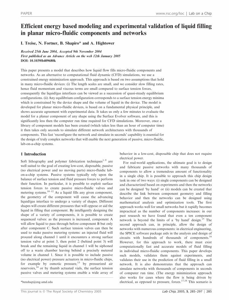
Efficient energy based modeling and experimental validation of liquid fillingin planar micro-fluidic components and networks

I. Treise, N. Fortner, B. Shapiro* and A. Hightower

Received 25th June 2004, Accepted 9th November 2004

First published as an Advance Article on the web 12th January 2005

DOI: 10.1039/b409680k

This paper presents a model that describes how liquid flow fills micro-fluidic components and

networks. As an alternative to computational fluid dynamic (CFD) simulations, we use a

constrained energy minimization approach. This approach is based on two assumptions that hold

in many micro-fluidic devices: (i) The length scales are small, and we consider slow filling rates,

hence fluid momentum and viscous terms are small compared to surface tension forces,

consequently the liquid/gas interfaces can be viewed as a succession of quasi-steady equilibrium

configurations. (ii) Any equilibrium configuration corresponds to a surface tension energy minima

which is constrained by the device shape and the volume of liquid in the device. The model is

developed for planar micro-fluidic devices, is based on a fundamental physical principle, and

shows accurate agreement with experimental data. It takes us only a few minutes to evaluate the

model for a planar component of any shape using the Surface Evolver software, and this is

significantly less then the computer run time required for CFD simulations. Moreover, once a

library of component models has been created (which takes less than an hour of computer time)

it then takes only seconds to simulate different network architectures with thousands of

components. This fast ‘reconfigure the network and simulate in seconds’ capability is essential for

the design of truly complex networks that will enable the next generation of passive, micro-fluidic,

lab-on-a-chip systems.

1 Introduction

Soft lithography and polymer fabrication techniques1–9 are

well suited to the goal of creating low-cost, disposable, passive

(no electrical power and no moving parts) micro-fluidic lab-

on-a-chip systems. Passive systems typically rely upon the

balance of surface tension and fluid pressure forces to perform

their function. In particular, it is possible to exploit surface

tension forces to create passive micro-fluidic valves and

metering systems.10–12 As a liquid fills any given component,

the geometry of the component will cause the advancing

liquid/gas interface to undergo a variety of shapes. Different

shapes will create different pressures that will oppose or aid the

liquid in filling that component. By intelligently designing the

shape of a variety of components, it is possible to create

sequenced valves: as the pressure is increased, component A

will allow liquid to pass through before component B but only

after component C. Such surface tension valves can then be

used to make passive metering systems: an injected fluid will

proceed along channel 1 until it encounters a strong surface

tension valve at point 3, then point 2 (behind point 3) will

break and the remaining liquid in channel 1 will be siphoned

off to a waste chamber leaving behind a precisely metered

volume in channel 1. Since it is possible to include passive

(no electrical power) pressure actuators in micro-fluidic chips,

for example by osmotic pressure,13 by pressurized air

reservoirs,14 or by thumb actuated vials, the surface tension

passive valves and metering systems enable a wide array of

behavior in a low-cost, disposable chip that does not require

electrical power.

For real-world applications, the ultimate goal is to design

and fabricate passive networks with many thousands of

components to allow a tremendous amount of functionality

in a single chip. It is possible to approach this chip design

task in one of two ways: (i) single components can be designed

and characterized based on experiments and then the networks

can be designed ‘by hand’ or (ii) models can be created that

describe the link between component geometry and filling

behavior and then the networks can be designed using

mathematical analysis and optimization tools. The first

approach works well for small networks but it rapidly becomes

impractical as the number of components increases: in our

past research we have found that even a ten component

network is beyond the limits of a ‘by hand’ design.15 The

second approach can, in principle, allow the design of

networks with numerous components: in electrical engineering,

the SPICE software package aids in the analysis and design of

circuits with hundreds of thousands of components.16

However, for this approach to work, there must exist

computationally fast and accurate models of fluid filling

in individual micro-fluidic components. This paper develops

such models, validates them against experiments, and

validates their use in the prediction of fluid filling in a small

network. It is also demonstrates that the approach can

simulate networks with thousands of components in seconds

of computer run time. (The energy minimization approach

also works for cases where the flow is being driven by

electrical, as opposed to pressure, forces.17,18 This scenario is*[email protected]

PAPER www.rsc.org/loc | Lab on a Chip

This journal is � The Royal Society of Chemistry 2005 Lab Chip, 2005, 5, 285–297 | 285

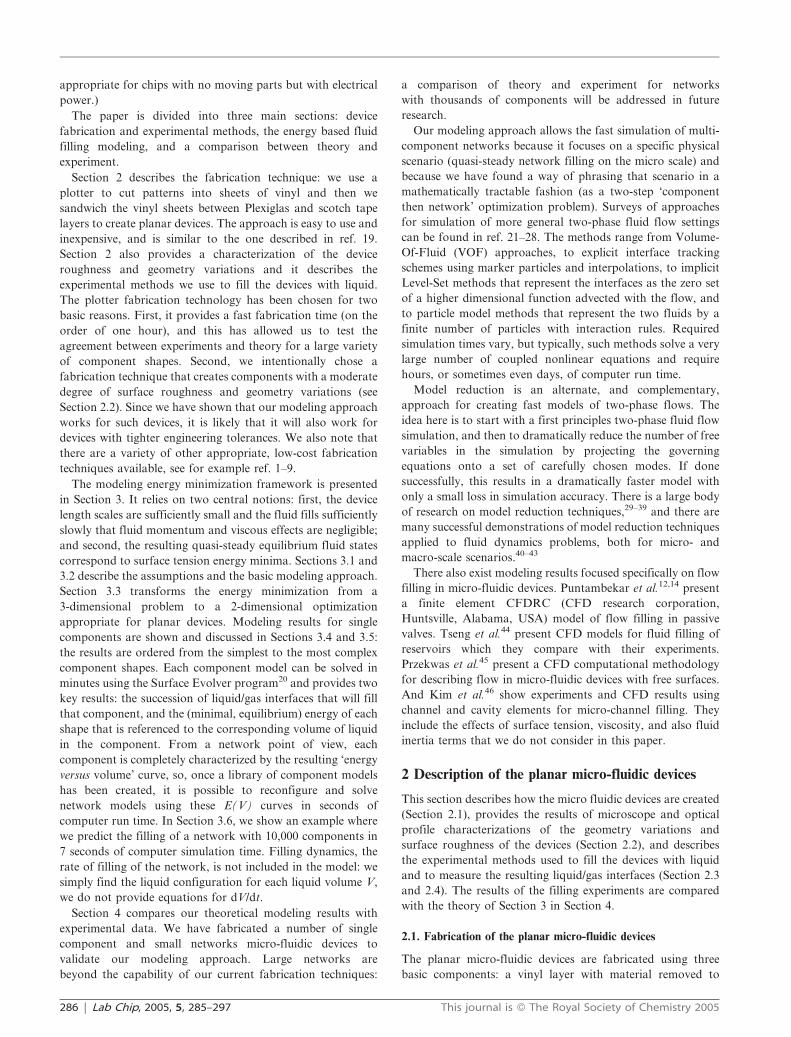
appropriate for chips with no moving parts but with electrical

power.)

The paper is divided into three main sections: device

fabrication and experimental methods, the energy based fluid

filling modeling, and a comparison between theory and

experiment.

Section 2 describes the fabrication technique: we use a

plotter to cut patterns into sheets of vinyl and then we

sandwich the vinyl sheets between Plexiglas and scotch tape

layers to create planar devices. The approach is easy to use and

inexpensive, and is similar to the one described in ref. 19.

Section 2 also provides a characterization of the device

roughness and geometry variations and it describes the

experimental methods we use to fill the devices with liquid.

The plotter fabrication technology has been chosen for two

basic reasons. First, it provides a fast fabrication time (on the

order of one hour), and this has allowed us to test the

agreement between experiments and theory for a large variety

of component shapes. Second, we intentionally chose a

fabrication technique that creates components with a moderate

degree of surface roughness and geometry variations (see

Section 2.2). Since we have shown that our modeling approach

works for such devices, it is likely that it will also work for

devices with tighter engineering tolerances. We also note that

there are a variety of other appropriate, low-cost fabrication

techniques available, see for example ref. 1–9.

The modeling energy minimization framework is presented

in Section 3. It relies on two central notions: first, the device

length scales are sufficiently small and the fluid fills sufficiently

slowly that fluid momentum and viscous effects are negligible;

and second, the resulting quasi-steady equilibrium fluid states

correspond to surface tension energy minima. Sections 3.1 and

3.2 describe the assumptions and the basic modeling approach.

Section 3.3 transforms the energy minimization from a

3-dimensional problem to a 2-dimensional optimization

appropriate for planar devices. Modeling results for single

components are shown and discussed in Sections 3.4 and 3.5:

the results are ordered from the simplest to the most complex

component shapes. Each component model can be solved in

minutes using the Surface Evolver program20 and provides two

key results: the succession of liquid/gas interfaces that will fill

that component, and the (minimal, equilibrium) energy of each

shape that is referenced to the corresponding volume of liquid

in the component. From a network point of view, each

component is completely characterized by the resulting ‘energy

versus volume’ curve, so, once a library of component models

has been created, it is possible to reconfigure and solve

network models using these E(V) curves in seconds of

computer run time. In Section 3.6, we show an example where

we predict the filling of a network with 10,000 components in

7 seconds of computer simulation time. Filling dynamics, the

rate of filling of the network, is not included in the model: we

simply find the liquid configuration for each liquid volume V,

we do not provide equations for dV/dt.

Section 4 compares our theoretical modeling results with

experimental data. We have fabricated a number of single

component and small networks micro-fluidic devices to

validate our modeling approach. Large networks are

beyond the capability of our current fabrication techniques:

a comparison of theory and experiment for networks

with thousands of components will be addressed in future

research.

Our modeling approach allows the fast simulation of multi-

component networks because it focuses on a specific physical

scenario (quasi-steady network filling on the micro scale) and

because we have found a way of phrasing that scenario in a

mathematically tractable fashion (as a two-step ‘component

then network’ optimization problem). Surveys of approaches

for simulation of more general two-phase fluid flow settings

can be found in ref. 21–28. The methods range from Volume-

Of-Fluid (VOF) approaches, to explicit interface tracking

schemes using marker particles and interpolations, to implicit

Level-Set methods that represent the interfaces as the zero set

of a higher dimensional function advected with the flow, and

to particle model methods that represent the two fluids by a

finite number of particles with interaction rules. Required

simulation times vary, but typically, such methods solve a very

large number of coupled nonlinear equations and require

hours, or sometimes even days, of computer run time.

Model reduction is an alternate, and complementary,

approach for creating fast models of two-phase flows. The

idea here is to start with a first principles two-phase fluid flow

simulation, and then to dramatically reduce the number of free

variables in the simulation by projecting the governing

equations onto a set of carefully chosen modes. If done

successfully, this results in a dramatically faster model with

only a small loss in simulation accuracy. There is a large body

of research on model reduction techniques,29–39 and there are

many successful demonstrations of model reduction techniques

applied to fluid dynamics problems, both for micro- and

macro-scale scenarios.40–43

There also exist modeling results focused specifically on flow

filling in micro-fluidic devices. Puntambekar et al.12,14 present

a finite element CFDRC (CFD research corporation,

Huntsville, Alabama, USA) model of flow filling in passive

valves. Tseng et al.44 present CFD models for fluid filling of

reservoirs which they compare with their experiments.

Przekwas et al.45 present a CFD computational methodology

for describing flow in micro-fluidic devices with free surfaces.

And Kim et al.46 show experiments and CFD results using

channel and cavity elements for micro-channel filling. They

include the effects of surface tension, viscosity, and also fluid

inertia terms that we do not consider in this paper.

2 Description of the planar micro-fluidic devices

This section describes how the micro fluidic devices are created

(Section 2.1), provides the results of microscope and optical

profile characterizations of the geometry variations and

surface roughness of the devices (Section 2.2), and describes

the experimental methods used to fill the devices with liquid

and to measure the resulting liquid/gas interfaces (Section 2.3

and 2.4). The results of the filling experiments are compared

with the theory of Section 3 in Section 4.

2.1. Fabrication of the planar micro-fluidic devices

The planar micro-fluidic devices are fabricated using three

basic components: a vinyl layer with material removed to

286 | Lab Chip, 2005, 5, 285–297 This journal is � The Royal Society of Chemistry 2005

create micro-channels, a Plexiglas backing with inlet and outlet

holes for the fluid, and an adhesive tape covering layer. These

components are assembled in a sandwich. The overall

approach is similar to the one outlined in ref. 19.

The fabrication begins by creating the channel design for the

middle layer of the sandwich that is a 70 mm thin vinyl film

(Oracle Economy distributed by SignWarehouse). The vinyl

has adhesive on one side and is lightly adhered to a silicone-

coated paper from which it is easily removed. Once the micro-

channel design is drawn in a Windows application called

SignGo (by Wissen UK Inc.), it is transferred to a vinyl cutter

(120 Vinyl Express LYNX2 Desktop, distributed by

SignWarehouse). The cutter has accurate control, which allows

lines, circles, and arcs to be cut smoothly into the vinyl.

By controlling the cut speed, the blade cutting angle (choices

are 30u, 45u, and 60u), and by adjusting the force on the blade,

the cutter can cut materials with a maximum thickness of

0.03 inches (0.762 mm). Plotter motions are accurate within a

few microns, but are limited to x and y changes of 30 mm by the

resolution of the SignGo software. To guarantee a high quality

cut, the blade has to be changed regularly to limit the effects of

blade abrasion.

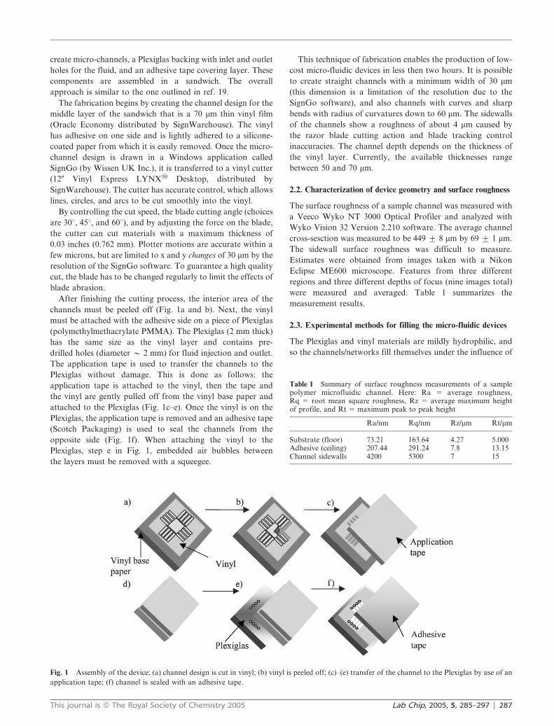
After finishing the cutting process, the interior area of the

channels must be peeled off (Fig. 1a and b). Next, the vinyl

must be attached with the adhesive side on a piece of Plexiglas

(polymethylmethacrylate PMMA). The Plexiglas (2 mm thick)

has the same size as the vinyl layer and contains pre-

drilled holes (diameter y 2 mm) for fluid injection and outlet.

The application tape is used to transfer the channels to the

Plexiglas without damage. This is done as follows: the

application tape is attached to the vinyl, then the tape and

the vinyl are gently pulled off from the vinyl base paper and

attached to the Plexiglas (Fig. 1c–e). Once the vinyl is on the

Plexiglas, the application tape is removed and an adhesive tape

(Scotch Packaging) is used to seal the channels from the

opposite side (Fig. 1f). When attaching the vinyl to the

Plexiglas, step e in Fig. 1, embedded air bubbles between

the layers must be removed with a squeegee.

This technique of fabrication enables the production of low-

cost micro-fluidic devices in less then two hours. It is possible

to create straight channels with a minimum width of 30 mm

(this dimension is a limitation of the resolution due to the

SignGo software), and also channels with curves and sharp

bends with radius of curvatures down to 60 mm. The sidewalls

of the channels show a roughness of about 4 mm caused by

the razor blade cutting action and blade tracking control

inaccuracies. The channel depth depends on the thickness of

the vinyl layer. Currently, the available thicknesses range

between 50 and 70 mm.

2.2. Characterization of device geometry and surface roughness

The surface roughness of a sample channel was measured with

a Veeco Wyko NT 3000 Optical Profiler and analyzed with

Wyko Vision 32 Version 2.210 software. The average channel

cross-sesction was measured to be 449 ¡ 8 mm by 69 ¡ 1 mm.

The sidewall surface roughness was difficult to measure.

Estimates were obtained from images taken with a Nikon

Eclipse ME600 microscope. Features from three different

regions and three different depths of focus (nine images total)

were measured and averaged. Table 1 summarizes the

measurement results.

2.3. Experimental methods for filling the micro-fluidic devices

The Plexiglas and vinyl materials are mildly hydrophilic, and

so the channels/networks fill themselves under the influence of

Fig. 1 Assembly of the device; (a) channel design is cut in vinyl; (b) vinyl is peeled off; (c)–(e) transfer of the channel to the Plexiglas by use of an

application tape; (f) channel is sealed with an adhesive tape.

Table 1 Summary of surface roughness measurements of a samplepolymer microfluidic channel. Here: Ra 5 average roughness,Rq 5 root mean square roughness, Rz 5 average maximum heightof profile, and Rt 5 maximum peak to peak height

Ra/nm Rq/nm Rz/mm Rt/mm

Substrate (floor) 73.21 163.64 4.27 5.000Adhesive (ceiling) 207.44 291.24 7.8 13.15Channel sidewalls 4200 5300 7 15


capillary forces. In order to fill the channels in this way, the

water is injected into the holes of the Plexiglas which serve as

fluid reservoirs. After the fluid comes in contact with the

bottom layer of the device it slowly creeps along the walls of

the channels towards the exit. Typically, we use red food color

(Mc Cormick), whose main ingredients are water, propylene

glycol and a red dye to visualize the liquid and to see the

progressing liquid/gas fronts in the devices. A camera records

the motion of the colored fluid for subsequent analysis and

interpretation.

Before first using the device, it is important to remove

all dust particles in the channels which deposit during

fabrication. The cleaning proceeds by flushing the channels

with ethanol using a vacuum pump and waiting until

the channels are dry. Each device can be used multiple times,

but it is necessary to clean the device with ethanol after

each use.

2.4. Experimental methods for measuring liquid/gas interfaces in

the devices

Liquid/gas interfaces are measured using a CCD Camera

(Digital Camera Vision Components Ettlingen, Germany)

with an integrated DSP (Digital Signal Processor). The DSP is

dedicated to Image Processing and to transferring the pixilated

image data from the camera to the host computer. The camera

is mounted on a Bausch & Lomb microscope with a

magnification of 660 (objectives: 3X, 20X). Using a Video

Converter (StarTech.com) and an external USB TV connec-

tion (AverMedia) the experiment images can be recorded as

AVI files. These AVI files are imported into Matlab and are

processed using the image processing toolbox to find the

location and shape of the liquid/gas interfaces.

To find the (effective planar) surface tension coefficient for

the devices, when filled with water or with any other liquid, we

compare the liquid/gas filling fronts in a simple channel

experiment with the minimum energy model of Section 3. This

technique selects the surface tension coefficient of eqn. (3) that

bests fits the experimental data. This process is carried out

one time for each type of fluid (the same solid materials

are used for all our devices). This comparison method is

equivalent to directly measuring the contact angle found in the

planar devices but it is more accurate and it directly provides

the single unknown material dependent coefficient c that is

necessary for our modeling.

As a way to check our values for the planar surface tension

coefficient we also measured the contact angles of the liquid

(deionized water and methanol) with respect to the floor,

ceiling, and wall materials of our devices. The angles were

measured using the sessile drop method in air using a

goniometer coupled with an American Optical AO569 Stereo

Microscope and a digital camera Oympus C-4000 digital

camera. Two droplets were tested and averaged for each

surface. The wall contact angle measurements are suspect

because we had to stack up 60 layers of vinyl sheets in order to

get a sufficiently large area to perform the tests, and it is quite

likely that the interface created in this way is not a true

reflection of the channel wall surface tension characteristics

found in our devices. Nevertheless, the value we get for the

planar surface tension coefficient c of eqn. (3) is consistent

with the experimental values in Section 4.

3. The energy based component filling modelingframework

Our modeling goal is to find the shape of the liquid/gas

interfaces as the liquid fills planar, single or multiple,

components with arbitrary geometries. Further, we desire a

model that is sufficiently accurate to enable engineering

analysis and design but that evaluates adequately fast to

enable the simulation of thousands of coupled components—

our end goal is to simulate, analyze, and design the filling of

complex micro-fluidic networks.

The energy minimization modeling approach that we use is

based on two observations. First, the network is filled slowly

by capillary forces hence we treat the propagating liquid/gas

interfaces as a succession of quasi-steady equilibrium con-

figurations. The succession of equilibrium states is para-

meterized by the amount of liquid in the device: each

equilibrium state corresponds to a specific volume of liquid.

Second, stable (or unstable) equilibrium shapes correspond to

minima (or maxima/saddles) of the surface tension potential

energy.47–49 This means that we can phrase the equilibrium

shape problem as an optimization problem with filled volume

and device geometry constraints. We are able to solve this

optimization task quickly and accurately.

3.1. The filling rate and the validity of the quasi-steady

assumption

The validity of our quasi-steady assumptions depends on size

of the micro-fluidic network and the rate of filling. To estimate

the permissible rate of filling of the network before the quasi-

steady model fails, we proceed as follows. The analysis below

holds either for self-filling by capillary forces or for forced

filling via a syringe or a pump. We consider a network with n

channels of average length l and radius r. For such a network,

the viscous forces, and hence the order of magnitude of

any applied pressure/momentum forces that are used to

drive the flow at a prescribed volume flow rate, scale as

Fvisc y (mU/r)Avisc y (mU/r)(2prnl) y pmnlU where m is the

viscosity of the fluid, U is the velocity of the fluid, and

Avisc 5 2prnl is the contact area over which the viscous stresses

act. The quasi-steady theory will fail when the momentum

forces first approach the size of the surface tension

forces inside each channel. The surface tension forces scale

as FSTy A s/R y psr where A 5 pr2 is the cross section

area and R y r is the radius of curvature of the interface.

The momentum forces are comparable to the viscous

forces. Hence the quasi-steady theory is valid whenFvisc

FST~

nl

r

mU

s~

nl

rCa%1 where Ca 5 mU/s is the capillary

number, or equivalently, when U%r

nl

s

m. Water has a viscosity

of m 5 1023 kg ms21 and the water/air surface tension

coefficient is s 5 0.72 6 1023 kg s22,47 so for the filling of

micro-fluidic networks with water displacing air we require

U % (r/nl) 0.72 m s21 for the quasi-steady theory to hold. For

the networks considered in this paper, we have channels with


approximate length l y 1 cm and radius r y 100 mm, and we

treat up to ten channels at once n ¡ 10. Thus we need

U % 0.72 mm s21 which means it would take us about one

or two minutes to fill a network with channels of length 1 cm

(120 s is much greater than the 1 cm/0.072 cm s21 5 13.8 s ). In

the experiments, we fill the networks in about five to seven

minutes to guarantee that the quasi-steady assumption remains

valid. For future, faster network filling applications we are

extending our methods to include computationally cheap

(reduced order) models of viscous effects. This will enable us

to move beyond the quasi-steady assumption used in this paper.

We also note that there are friction forces due to the moving

contact line that we do not consider here. It is expected that

such forces will become important near the walls, floor, and

ceiling, and they will have a substantial overall effect on the

liquid shape only for devices with very small filling lengths.

For a description of moving contact line friction forces see, for

example ref. 50–52.

3.2. The basic approach: minimization of the surface tension

potential energy under device geometry and enclosed liquid

volume constraints

At every instant in time the liquid/gas interface equilibrium

configurations are viewed as the minima of the surface tension

potential energy. Viewing spherical liquid droplet shapes and

interface contact angles as minimum energy surfaces is

customary and it is consistent with the methods described in

ref. 20,47–49. Our approach of viewing any equilibrium liquid/

gas interface as an energy minimum is a natural extension, and

it is a subset of the far more general concept that all

equilibrium configurations, for almost any kind of system,

correspond to energy minima.53 As noted by Feynman,53 net

forces are the derivatives of the energy with respect to shape

parameters, so the forces balance if and only if the system

potential energy is at a stationary point.

Our main contribution is to effectively apply the above

energy minimization idea in complex (but planar) devices and

networks. We do this by finding the interface shape that

minimizes the surface tension energy cost subject to constraints

imposed by the device geometry and by the amount of fluid

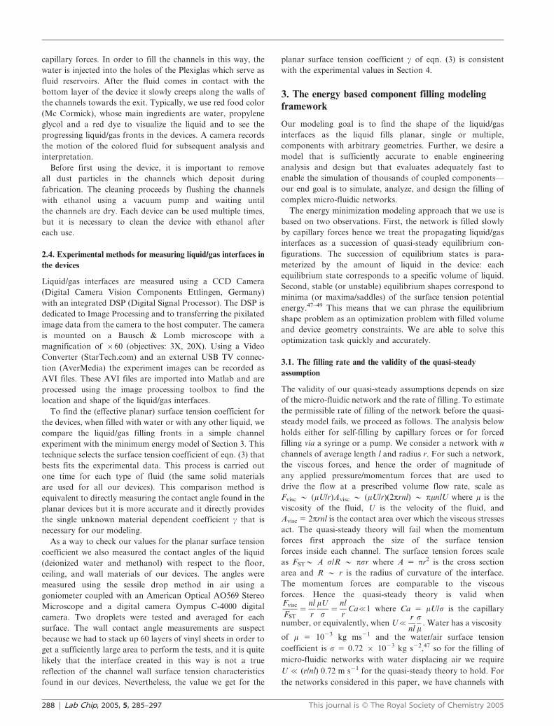
that has been injected or sucked into the device. For example,

if we have a twisted T geometry which contains thirty

microliters of liquid, we find the liquid/gas interface shape by

solving an optimization problem that minimizes the surface

tension energy subject to the constraints that the interface be

confined inside the twisted T and encloses exactly thirty

microliters of liquid. At the next instant in time we repeat the

process for thirty one microliters of fluid. A schematic of this

approach is shown in Fig. 2.

To do the above we must define the potential energy of the

micro-fluidic systems as a function of interface shapes. The

potential energy we consider consists of surface tension effects

only. Gravity effects are ignored due to the small size of the

devices. As in ref. 47,48, we model the energy per unit area of

each liquid/gas, liquid/solid, and solid/gas interface via a

material dependent surface tension coefficient. This gives the

potential energy as

E~

ðL\G

sLGdALGz

ðL\S

sLSdALSz

ðS\G

sSGdASG (1)

where S, L, and G are the domains in three-dimensional space

occupied by solid, liquid, and gas phase respectively, <

denotes their intersections (so L<S is the two-dimensional

liquid/solid interface), and sAB denotes the associated inter-

facial potential energy per unit area. The surface tension

energy formulation of eqn. (1) is acceptable so long as the

device length scale is large compared to the interface thickness.

This is certainly the case in our networks with micrometer

sized components.

3.3. Rephrasing the energy optimization problem in two spatial

dimensions

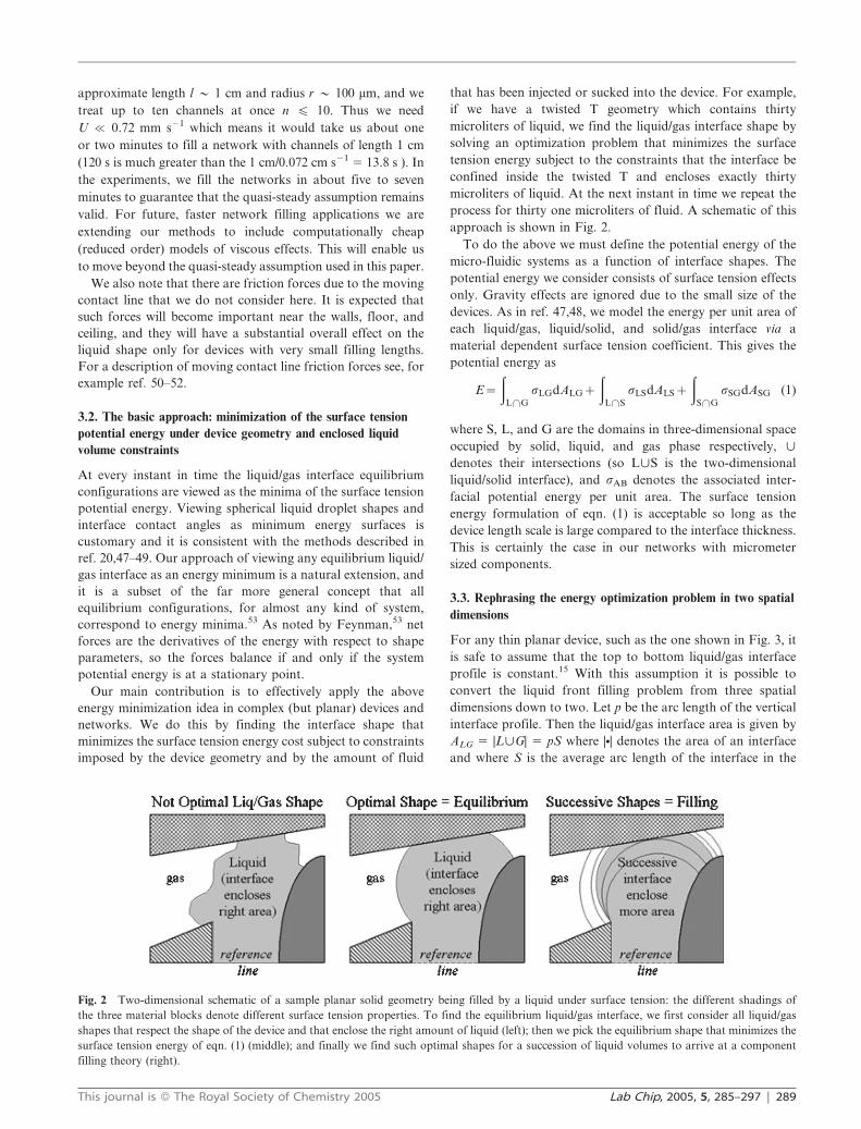
For any thin planar device, such as the one shown in Fig. 3, it

is safe to assume that the top to bottom liquid/gas interface

profile is constant.15 With this assumption it is possible to

convert the liquid front filling problem from three spatial

dimensions down to two. Let p be the arc length of the vertical

interface profile. Then the liquid/gas interface area is given by

ALG 5 |L<G| 5 pS where |N| denotes the area of an interface

and where S is the average arc length of the interface in the

Fig. 2 Two-dimensional schematic of a sample planar solid geometry being filled by a liquid under surface tension: the different shadings of

the three material blocks denote different surface tension properties. To find the equilibrium liquid/gas interface, we first consider all liquid/gas

shapes that respect the shape of the device and that enclose the right amount of liquid (left); then we pick the equilibrium shape that minimizes the

surface tension energy of eqn. (1) (middle); and finally we find such optimal shapes for a succession of liquid volumes to arrive at a component

filling theory (right).


horizontal plane (see, for example, Fig. 3). Here S varies as

the liquid fills the component but p remains constant. Since the

liquid/air surface tension coefficient is assumed constant, this

reduced the first term in the potential energy of eqn. (1) toÐL\G

sLGdALG~sLGALG~sLGpS. Likewise it is possible to

rewrite the liquid/solid and solid/gas potential energy terms

solely in terms of horizontal dimensions. For example, in the

L-corner, the wetted vertical liquid/wall surface areas are given

by hD1 and h D2 where D1 and D2 are as shown in Fig. 3 and h

is the vertical distance between the floor and the ceiling. The

gas/wall surface areas are simply the total available wall areas

minus the wetted liquid/wall areas. Finally, the floor–ceiling/

liquid and floor–ceiling/gas contact areas are irrelevant to the

shape energy minimization and they can be dropped from

the energy cost. This is because, at any moment in time, the

volume of liquid contained inside the device is treated as a

constant and is given by V 5 hALS:FS, where ALS:FC is the

contact area of the liquid with the floor and the ceiling. Since

this floor/liquid plus ceiling/liquid contact area only depends

on the amount of liquid currently contained inside the device,

it is independent of the horizontal shape of the liquid/gas

interface, and it can be dropped from the energy optimization

cost.

The surface tension energy of eqn. (1) can now be rewritten

in two spatial dimensions as

E2D 5 S + c1D1+ … + ckDk (2)

(5S + cD if all walls are of the same material)

where S is the mean horizontal arc length of the liquid/gas

interface, and D1, D2, … ,Dk are the wetted lengths of walls

1,2,…,k respectively. (For the planar L-corner, D1 and D2 are

as shown in Fig. 3.) The parameters c1, c2, … ck are non-

dimensional, material dependent, ratios of surface tension and

geometry parameters. Specifically, for the jth wall:

cj 5 h(sLS:Wj 2 sGS:Wj)/psLG (3)

In our devices all walls are made out of a single type of

material hence c1 5 c2 5 … 5 ck 5 c. We identify the single

missing coefficient c by finding the value c that provides the

best agreement between a straight channel experiment and a

straight channel energy model. The parameter c is related to

the observed contact angle in the horizontal plane by the

analog of the Young equation c 5 2cos h2D.47 Thus eqn. (3)

gives the contact angle in the horizontal plane as a function of

the surface tension coefficients of the Plexiglas, vinyl, and the

adhesive tape materials. In our devices, h2D varies between

105u and 112u degrees depending on the polymer manufac-

turer, handling, and experimental conditions that affect

material and surface properties, surface roughness, tempera-

ture, and humidity.

3.4. Filling of a planar L-corner

Except for a straight channel where the filling is trivial to

predict, the planar L-corner is the simplest possible geometry

that can be considered. Detailed results for this case have been

presented in our conference paper.15 Below we briefly

summarize the key results.

A cut away view of the planar L-corner geometry is shown

in Fig. 3. As a special case of eqn. (2), the surface tension

energy is given by E2D 5 S + c1D1 + c2D2. We must minimize

this energy subject to the liquid volume and device geometry

constraints. The minimization is done in two parts. First, for

any D1 and D2 we minimize the shape of a liquid/gas interface

pinned at the D1 and D2 lengths. By the calculus of variations54

we know that a circular arc is the required optimal shape

because it minimizes arc length subject to an enclosed area

constraint. The radius of this arc is uniquely determined by D1,

D2, and by the amount of liquid that has been injected or

sucked into the device at any time. Second, we find the optimal

D1 and D2 lengths. In ref. 15 we parameterize D1 and D2 by the

length 2l and orientation angle h of the line segment between

the arc starting and ending point since this provides a

smoother parameterization of the energy cost then the D1

and D2 parameterization.

The L-corner surface tension energy E2D 5 S + c1D1 + c2D2

is now a function of l and h only. However, not all (l, h) pairs

are permitted: some pairs violate the geometry of the device

(the arc intersects the walls at multiple points or fails to span

the channel), and some pairs violate enclosed area require-

ments (for these (l, h) pairs the arc radius cannot be chosen in a

way that respects the devices geometry and encloses the correct

amount of liquid). The geometric constraints on l and h are

Fig. 3 An L-corner planar geometry. Due to the small vertical height of the device, a liquid/gas interface moving through this geometry will have a

constant vertical interface shape: the interface shape will vary in the horizontal plane only.


derived analytically in ref. 15. The resulting (l*, h*) energy

minimum corresponds to the equilibrium shape of the liquid/

gas interface at a prescribed liquid volume. Using a gradient

descent algorithm it takes about 2 seconds to find any such

equilibrium front using Matlab on a desktop personal

computer. By finding a succession of optimal (l*, h*) pairs

for increasing liquid volumes, we arrive at an L-corner filling

theory. As shown in ref. 15 the agreement between theory and

experiment for the L-corner is excellent.

It is important to compare our approach above with the two

standard approaches of computational fluid dynamic (CFD)

and stand alone contact angle methods. CFD approaches

require a discretization of the (two-phase) Navier Stokes or

Stokes fluid equation along with the tracking and computation

of forces on a moving liquid/gas boundary. This is computa-

tionally expensive. A coarse 2-dimensional CFD simulation

for a planar component might have 100 by 100 grid points

with 3 variables (u, v, P) per node. That is a total of 30,000

equations that must be solved simultaneously for each time

step. To better resolve the liquid/gas curvature, a mesh of a

1000 by a 1000 grid points may be needed: this yields 3 million

equations. For this reason, Stokes flow two-phase simulations

carried out in our laboratory for the L-corner geometry take

two hours of computer run time per component. Simulation

times quoted in the literature vary from hours to days. By

comparison, the planar energy minimization proceeds by

optimizing a surface (a curve) that is adequately defined by 2

variables for the L-corner and by 20 to 40 points for other

component shape. Thus we iterate on less then 40 equations to

find the interface at each time. Our energy minimization

approach therefore takes seconds for the L-corner, minutes for

more complex component shapes, and by using a two-stage

approach, allows the simulation of networks in seconds.

Contact angle approaches specify the angle between the

liquid/gas interface and the solid surface. If used on their own

independently of CFD computations, then they are computa-

tionally trivial to implement but it is not clear how to use them

to find liquid/gas filling fronts in non-trivial device geometries.

This is true for a number of reasons that we list from the least

to the most serious. First, one requires an equation to translate

the three-dimensional contact angles (of water in air on vinyl,

on Plexiglas, and on scotch tape) into one planar two-

dimensional contact angle (see the discussion preceding

eqn. (3) ). This issue is minor: it is possible to circumvent it

by simply measuring the contact angle in the planar

geometries. Second, the contact angle condition is undefined

or cannot be true at corners, at lines of symmetry, and at

points where the liquid/gas front first impinges on a new solid

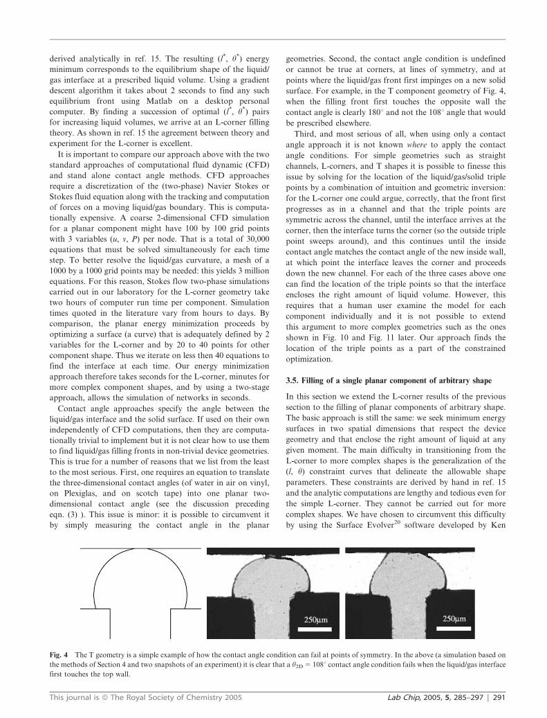
surface. For example, in the T component geometry of Fig. 4,

when the filling front first touches the opposite wall the

contact angle is clearly 180u and not the 108u angle that would

be prescribed elsewhere.

Third, and most serious of all, when using only a contact

angle approach it is not known where to apply the contact

angle conditions. For simple geometries such as straight

channels, L-corners, and T shapes it is possible to finesse this

issue by solving for the location of the liquid/gas/solid triple

points by a combination of intuition and geometric inversion:

for the L-corner one could argue, correctly, that the front first

progresses as in a channel and that the triple points are

symmetric across the channel, until the interface arrives at the

corner, then the interface turns the corner (so the outside triple

point sweeps around), and this continues until the inside

contact angle matches the contact angle of the new inside wall,

at which point the interface leaves the corner and proceeds

down the new channel. For each of the three cases above one

can find the location of the triple points so that the interface

encloses the right amount of liquid volume. However, this

requires that a human user examine the model for each

component individually and it is not possible to extend

this argument to more complex geometries such as the ones

shown in Fig. 10 and Fig. 11 later. Our approach finds the

location of the triple points as a part of the constrained

optimization.

3.5. Filling of a single planar component of arbitrary shape

In this section we extend the L-corner results of the previous

section to the filling of planar components of arbitrary shape.

The basic approach is still the same: we seek minimum energy

surfaces in two spatial dimensions that respect the device

geometry and that enclose the right amount of liquid at any

given moment. The main difficulty in transitioning from the

L-corner to more complex shapes is the generalization of the

(l, h) constraint curves that delineate the allowable shape

parameters. These constraints are derived by hand in ref. 15

and the analytic computations are lengthy and tedious even for

the simple L-corner. They cannot be carried out for more

complex shapes. We have chosen to circumvent this difficulty

by using the Surface Evolver20 software developed by Ken

Fig. 4 The T geometry is a simple example of how the contact angle condition can fail at points of symmetry. In the above (a simulation based on

the methods of Section 4 and two snapshots of an experiment) it is clear that a h2D 5 108u contact angle condition fails when the liquid/gas interface

first touches the top wall.


Brakke. This software finds minimal energy surfaces in two

and three spatial dimensions subject to various costs and

constraints. Surface Evolver defines surface as a union of

triangles in three spatial dimensions or as a collection of line

segments in two dimensions, it then evolves the surface in the

direction of decreasing cost by using a (constrained) gradient

descent algorithm.

We have successfully used Surface Evolver to predict liquid/

gas filling fronts in our micro-fluidic components. The energy

to be minimized is given by eqn. (2) where c is the material

dependent surface tension coefficient defined in eqn. (3) . For

any component, we start the Surface Evolver optimization at

an arbitrary interface shape defined by just three vertices. The

first and last vertices are restricted to be at the component

walls that act as geometric constraints. Surface Evolver then

refines the shape of the interface by successively adding and

moving the vertices to minimize the energy cost while

enforcing both the geometry and imposed liquid volume

constraints. Once convergence is achieved we increase the

liquid volume and, using the previous solution as the new

initial interface, we find a new optimal solution. This provides

a succession of optimal liquid/gas interfaces that fill the

component. Each simulation takes about 2–3 min to find the

succession of fronts through simple geometries, more complex

geometries require 6–8 min. Surface Evolver cannot guarantee

that global energy minima have been found. However, for the

component shapes used here, all the energy minima are

physically meaningful and, to the best of our knowledge,

correspond to global energy minima. Below we show results

for a variety of planar components.

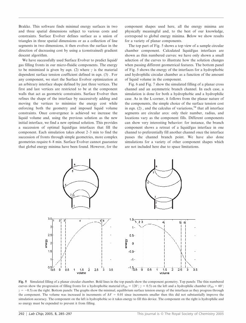
The top part of Fig. 5 shows a top view of a sample circular

chamber component. Calculated liquid/gas interfaces are

shown as thin numbered curves: we have only shown a small

selection of the curves to illustrate how the solution changes

when passing different geometrical features. The bottom panel

of Fig. 5 shows the energy of the interfaces for a hydrophobic

and hydrophilic circular chamber as a function of the amount

of liquid volume in the component.

Fig. 6 and Fig. 7 show the simulated filling of a planar cross

channel and an asymmetric branch channel. In each case, a

simulation is done for both a hydrophobic and a hydrophilic

case. As in the L-corner, it follows from the planar nature of

the components, the simple choice of the surface tension cost

in eqn. (2) , and the calculus of variations,54 that all interface

segments are circular arcs: only their number, radius, and

locations vary as the component fills. Different components

can show very interesting behavior: for instance, the branch

component shows a retreat of a liquid/gas interface in one

channel to preferentially fill another channel once the interface

passes the channel branch point. We have also done

simulations for a variety of other component shapes which

are not included here due to space limitations.

Fig. 5 Simulated filling of a planar circular chamber. Bold lines in the top panels show the component geometry. Top panels: The thin numbered

curves show the progression of filling fronts for a hydrophobic material (h2D 5 120u; c 5 0.5) on the left and a hydrophilic chamber (h2D 5 60u;c 5 20.5) on the right. Bottom panels: The graphs show the minimal, equilibrium surface tension energy of the interfaces as they progress through

the component. The volume was increased in increments of DV 5 0.01 since increments smaller then this did not substantially improve the

simulation accuracy. The component on the left is hydrophobic so it takes energy to fill this device. The component on the right is hydrophilic and

so energy must be expended to prevent it from filling.


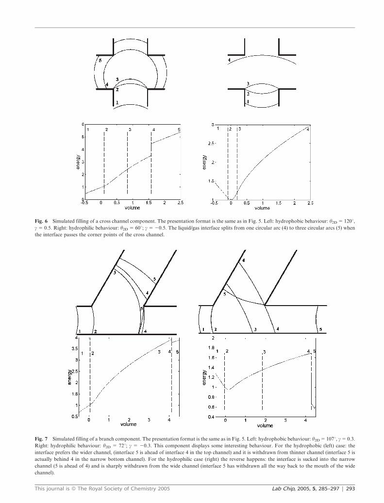
Fig. 6 Simulated filling of a cross channel component. The presentation format is the same as in Fig. 5. Left: hydrophobic behaviour: h2D 5 120u,c 5 0.5. Right: hydrophilic behaviour: h2D 5 60u; c 5 20.5. The liquid/gas interface splits from one circular arc (4) to three circular arcs (5) when

the interface passes the corner points of the cross channel.

Fig. 7 Simulated filling of a branch component. The presentation format is the same as in Fig. 5. Left: hydrophobic behaviour: h2D 5 107u, c 5 0.3.

Right: hydrophilic behaviour: h2D 5 72u; c 5 20.3. This component displays some interesting behaviour. For the hydrophobic (left) case: the

interface prefers the wider channel, (interface 5 is ahead of interface 4 in the top channel) and it is withdrawn from thinner channel (interface 5 is

actually behind 4 in the narrow bottom channel). For the hydrophilic case (right) the reverse happens: the interface is sucked into the narrow

channel (5 is ahead of 4) and is sharply withdrawn from the wide channel (interface 5 has withdrawn all the way back to the mouth of the wide

channel).


3.6 Filling of a hub network of planar components of arbitrary

shape

We now turn to modeling fluid filling in a network of

components. There are two possible ways to do this. The first

option is to perform a Surface Evolver simulation with

geometry constraints for the entire network: in this option

we simply replace the geometry of Fig. 5–7 with the geometry

of the entire network. This option is still less computationally

intensive then a CFD 2-phase simulation, but it is still fairly

expensive: a network with a hundred components would take

about 10 hours. Below, we discuss an alternate two-stage

approach that, once a library of component models has been

built up, can simulate networks with thousands of components

in seconds.

To simulate a network we must minimize the surface tension

energy of numerous interfaces across multiple components.

We already know how to find the minimal surface tension

energy of any single component using the methods of Section

3.5. The bottom panels of Fig. 5–7 show this equilibrium

energy as a function of the liquid volume in each component.

From a network point of view, these energy versus liquid

volume Ej(Vj) curves completely characterize the behavior

of each component. The total energy of a network with n

components is now given by the sum of individual component

energy versus volume functions

E 5 E1(V1) + E2(V2) + … + En(Vn). (4)

For example, we may consider a network made out of four

types of components (circular chambers, L-corners, cross

channels, and branch splitters) in which case each Ej(Vj)

function above would be one of four curves, two of which are

shown in Fig. 5 and Fig. 7. If the network included other types

of components we would pre-compute their energy versus

volume curves. Further, we know that the total network

volume is given by

V1 + V2 + … Vn 5 V. (5)

As the network fills, this total volume V goes from zero to

the maximum fluid volume that can be contained in the

network. The optimization task is to find the amount of

fluid in the components V1,V2,…,Vn that minimizes the

total surface tension energy of the network as the total

fluid goes from zero to its maximum value. Per the estimates

in Section 3.1, it is valid to treat the entire network as if it

were going through a succession of equilibrium states so

long as the self or imposed filling rate is sufficiently slow.

To find the equilibrium component filling volumes Vj’s as a

function of the total volume V we must solve the following

optimization:

min E~Pn

j~1 Ej Vj

� �subject to

Pnj~1 Vj~V : (6)

This is a standard nonlinear, multi-variable, scalar cost,

single constraint optimization.55 Here we have assumed that

all the components are connected to one central reservoir or

injection point. Networks with multiple hubs would require

multiple, interlinked sub-network component volume con-

straints. This would increase the number of constraints and

would increase the simulation time slightly.

In summary, the network model proceeds in two parts.

First, we generate a set of component simulations as in Section

3.5 using Surface Evolver. Since each component takes about 2

to 8 min to simulate, a network with thirty different types of

components would require a total computer run time of

between 1 and 4 hours. Second, once we have the Ej(Vj) curves

for all the components in the network, we solve the

optimization stated in eqn. (6) using a constrained gradient

descent algorithm. This takes seconds of computer run time

using Matlab on a personal computer. The architecture of

the network can now be changed and the behavior of the

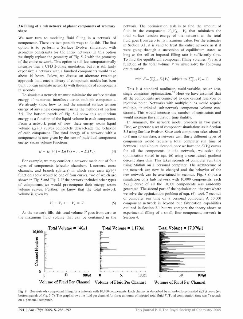
new network can be ascertained in seconds. Fig. 8 shows a

simulation of a hub network with 10,000 components: each

Ej(Vj) curve of all the 10,000 components was randomly

generated. The second part of the optimization, the part where

we solve the optimization problem of eqn. (6), took 7 seconds

of computer run time on a personal computer. A 10,000

component network is beyond our fabrication capabilities

outlined in Section 2.1 but we compare the theory above to

experimental filling of a small, four component, network in

Section 4.

Fig. 8 Quasi-steady component filling for a network with 10,000 components. Each channel is described by a randomly generated Ej(Vj) curve (see

bottom panels of Fig. 5–7). The graph shows the fluid per channel for three amounts of injected total fluid V. Total computation time was 7 seconds

on a personal computer.


4. Model validation: theory versus experiments

In this section, we compare experimental results attained using

the methods of Section 2 with the modeling approach

described in Section 3. Besides the geometry of the component

or network, the model requires two inputs, which are: the

volume of liquid in the component or network, and the surface

tension parameter c of eqn. (3) or equivalently the planar

contact angle h2D (c 5 2cos h2D). The volume of liquid inside

the component is known experimentally: we measure the filled

area using image processing techniques and then we multiply

this area by the depth of the device to find the contained liquid

volume. The c parameter of eqn. (3) depends on the height of

the planar device and the type of solid and liquid materials

being used. It is determined one time beforehand by comparing

the theoretical prediction for the filling of a straight channel

with an experiment.

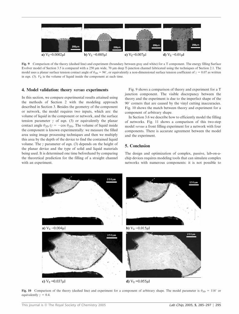
Fig. 9 shows a comparison of theory and experiment for a T

junction component. The visible discrepancy between the

theory and the experiment is due to the imperfect shape of the

90u corners that are caused by the vinyl cutting inaccuracies.

Fig. 10 shows the match between theory and experiment for a

component of arbitrary shape.

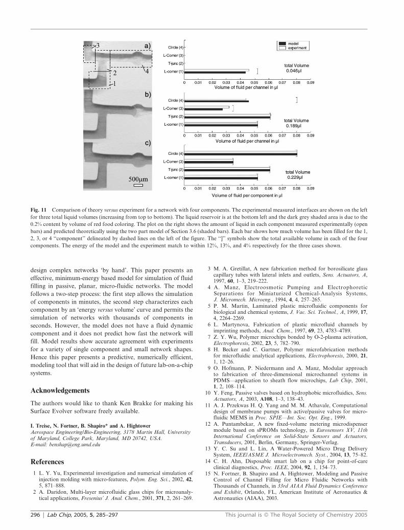
In Section 3.6 we describe how to efficiently model the filling

of networks. Fig. 11 shows a comparison of this two-step

model versus a front filling experiment for a network with four

components. There is accurate agreement between the model

and the experiment.

5. Conclusion

The design and optimization of complex, passive, lab-on-a-

chip devices requires modeling tools that can simulate complex

networks with numerous components: it is not possible to

Fig. 9 Comparison of the theory (dashed line) and experiment (boundary between gray and white) for a T component. The energy filling Surface

Evolver model of Section 3.5 is compared with a 250 mm wide, 70 mm deep T-junction channel fabricated using the techniques of Section 2.1. The

model uses a planar surface tension contact angle of h2D 5 94u, or equivalently a non-dimensional surface tension coefficient of c 5 0.07 as written

in eqn. (3). VE is the volume of liquid inside the component at each time.

Fig. 10 Comparison of the theory (dashed line) and experiment for a component of arbitrary shape. The model parameter is h2D 5 114u or

equivalently c 5 0.4.


design complex networks ‘by hand’. This paper presents an

effective, minimum-energy based model for simulation of fluid

filling in passive, planar, micro-fluidic networks. The model

follows a two-step process: the first step allows the simulation

of components in minutes, the second step characterizes each

component by an ‘energy versus volume’ curve and permits the

simulation of networks with thousands of components in

seconds. However, the model does not have a fluid dynamic

component and it does not predict how fast the network will

fill. Model results show accurate agreement with experiments

for a variety of single component and small network shapes.

Hence this paper presents a predictive, numerically efficient,

modeling tool that will aid in the design of future lab-on-a-chip

systems.

Acknowledgements

The authors would like to thank Ken Brakke for making his

Surface Evolver software freely available.

I. Treise, N. Fortner, B. Shapiro* and A. HightowerAerospace Engineering/Bio-Engineering, 3178 Martin Hall, Universityof Maryland, College Park, Maryland, MD 20742, USA.E-mail: [email protected]

References

1 L. Y. Yu, Experimental investigation and numerical simulation ofinjection molding with micro-features, Polym. Eng. Sci., 2002, 42,5, 871–888.

2 A. Daridon, Multi-layer microfluidic glass chips for microanaly-tical applications, Fresenius’ J. Anal. Chem., 2001, 371, 2, 261–269.

3 M. A. Gretillat, A new fabrication method for borosilicate glasscapillary tubes with lateral inlets and outlets, Sens. Actuators, A,1997, 60, 1–3, 219–222.

4 A. Manz, Electroosmotic Pumping and ElectrophoreticSeparations for Miniaturized Chemical-Analysis Systems,J. Micromech. Microeng., 1994, 4, 4, 257–265.

5 P. M. Martin, Laminated plastic microfluidic components forbiological and chemical systems, J. Vac. Sci. Technol., A, 1999, 17,4, 2264–2269.

6 L. Martynova, Fabrication of plastic microfluid channels byimprinting methods, Anal. Chem., 1997, 69, 23, 4783–4789.

7 Z. Y. Wu, Polymer microchips bonded by O-2-plasma activation,Electrophoresis, 2002, 23, 5, 782–790.

8 H. Becker and C. Gartner, Polymer microfabrication methodsfor microfluidic analytical applications, Electrophoresis, 2000, 21,1, 12–26.

9 O. Hofmann, P. Niedermann and A. Manz, Modular approachto fabrication of three-dimensional microchannel systems inPDMS—application to sheath flow microchips, Lab Chip, 2001,1, 2, 108–114.

10 Y. Feng, Passive valves based on hydrophobic microfluidics, Sens.Actuators, A, 2003, A108, 1–3, 138–43.

11 A. J. Przekwas H. Q. Yang and M. M. Athavale, Computationaldesign of membrane pumps with active/passive valves for micro-fluidic MEMS in Proc. SPIE—Int. Soc. Opt. Eng., 1999.

12 A. Puntambekar, A new fixed-volume metering microdispensermodule based on sPROMs technology, in Eurosensors XV, 11thInternational Conference on Solid-State Sensors and Actuators,Transducers, 2001, Berlin, Germany, Springer-Verlag.

13 Y. C. Su and L. Lin, A Water-Powered Micro Drug DeliverySystem, IEEE/ASME J. Microelectromech. Syst., 2004, 13, 75–82.

14 C. H. Ahn, Disposable smart lab on a chip for point-of-careclinical diagnostics, Proc. IEEE, 2004, 92, 1, 154–73.

15 N. Fortner, B. Shapiro and A. Hightower, Modeling and PassiveControl of Channel Filling for Micro Fluidic Networks withThousands of Channels, in 33rd AIAA Fluid Dynamics Conferenceand Exhibit, Orlando, FL, American Institute of Aeronautics &Astronautics (AIAA), 2003.

Fig. 11 Comparison of theory versus experiment for a network with four components. The experimental measured interfaces are shown on the left

for three total liquid volumes (increasing from top to bottom). The liquid reservoir is at the bottom left and the dark grey shaded area is due to the

0.2% content by volume of red food coloring. The plot on the right shows the amount of liquid in each component measured experimentally (open

bars) and predicted theoretically using the two part model of Section 3.6 (shaded bars). Each bar shows how much volume has been filled for the 1,

2, 3, or 4 ‘‘component’’ delineated by dashed lines on the left of the figure. The ‘‘]’’ symbols show the total available volume in each of the four

components. The energy of the model and the experiment match to within 12%, 13%, and 4% respectively for the three cases shown.


16 P. W. Tuinenga, SPICE : a guide to circuit simulation and analysisusing PSpice, 3rd edn., Prentice HallEnglewood Cliffs, N.J., 1995.

17 N. Fortner and B. Shapiro, Equilibrium and Dynamic Behavior ofMicro Flows Under Electrically Induced Surface TensionActuation Forces in The 2003 International Conference onMEMS, NANO, and Smart Systems (ICMEMS), 2003, Banff,Alberta, Canada.

18 B. Shapiro, Equilibrium Behavior of Sessile Drops under SurfaceTension, Applied External Fields, and Material Variations, J. Appl.Phys., 2003, 93, 9.

19 Y. Lin, Microfluidic Devices on Polymer Substrates forBioanalytical Applications, in IMRET3, 3rd InternationalConference On Microreaction Technology, 1999, Frankfurt,Germany.

20 K. Brakke, The Surface Evolver, Experimental Mathematics, 1992,1, 2, 141–165.

21 J. M. Floryan and H. Rasmussen, Numerical methods for viscousflows with moving boundaries, Appl. Mech. Rev., 1989, 42, 12.

22 J. M. Hyman, Numerical methods for tracking interfaces, Physica,1984, 12, D, 396–407.

23 J. J. Monaghan, Particle methods for hydrodynamics, Comput.Phys. Rep., 1985, 3, 71–124.

24 S. Osher and R. Fedkiw, Level Set Methods and Dynamic ImplicitSurfaces, Springer-Verlag, New York, 2003.

25 S. A. Sethian, Level Set Methods & Fast Marching Methods, 2ndedn., Cambridge University Press, 1999.

26 C. W. Hirt and B. D. Nichols, Volume of fluid (VOF) method forthe dynamics of free boundaries, J. Comput. Phys., 1981, 39,201–225.

27 R. P. Fedkiw, A non-oscillatory eulerian approach to interfaces inmulti-material flows (the ghost fluid method), Comput. Phys., 1999,152, 457–492.

28 R. Caiden, R. Fedkiw and C. Anderson, A Numerical Method forTwo Phase Flow Consisting of Separate Compressible andIncompressible Regions, J. Comput. Phys., 2001, 166, 1–27.

29 A. C. Antoulas, D. C. Sorensen and S. Gugercin, A survey ofmodel reduction methods for large-scale systems, Contemp. Math.,2001, 280, 193–219.

30 N. K. Sinha, Reduced-order models for linear systems in IEEEInternational Conference on Systems, Man and Cybernetics, IEEE,New York, NY, 1992.

31 D. Hinrichsen and H. W. Philippsen, Model reduction usingbalanced realizations, Automatisierungstechnik, 1990, 38, 11.

32 A. M. S. Dahshan,A. S. Fawzy and Y. A. E. Sawy, Comparisons ofseveral model reduction techniques. , IEEE, New York, NY, 1985.

33 S. Shokoohi, A survey of model reduction techniques for large-scalesystems, West Virginia University, Morgantown WV, USA,distributed by Western Periodicals Co., 1984.

34 N. K. Sinha and G. J. Lastman, Reduced order models forcomplex systems—a critical survey in IETE Technical Review,1990.

35 Y. G. Kevrekidis, Order Reduction for Nonlinear DynamicModels of Distributed Reacting Systems, J. Process Control,2000, 10, 177–184.

36 B. C. Moore, Principal component analysis in linear systems:controllability, observability, and model reduction, IEEE Trans.Automatic Control, 1981, AC-26, 17–32.

37 E. J. Grimme, Krylov Projection Methods for Model Reduction,PhD Thesis, ECE dept., University of Illinois at Urbana-Champaign, Urbana-Champaign, 1997.

38 T. Penzl, Algorithms for model reduction of large dynamical systems,2000, Sonderforschungsbereich 393, Numerische Simulation aufmassiv parallelen Rechern, TU Chemnitz 09107.

39 A. Bultheel and M. V. Barel, Pade techniques for model reductionin linear systems theory: a survey, J. Comput. Appl. Math., 1986,14, 3.

40 K. Willcox and J. Peraire, Balanced Model Reduction via theProper Orthogonal Decomposition in AIAA Computational FluidDynamics Conference, Anaheim, CA, 2001.

41 L. Sirovich, Turbulences and the dynamics of coherent structures,parts I & II, Quart. Appl. Math., 1987, 45, 561–571.

42 W. R. Graham, J. Peraire and K. Y. Tang, Optimal control ofvortex shedding using low order models—Part I: Open-loop modeldevelopment, J. Num. Meth. Engr., 1999, 44, 7, 945–972.

43 R. Qiao and N. R. Aluru, A compact model for electroosmoticflows in microfluidic devices, J. Micromech. Microeng., 2002, 12, 5,625–35.

44 F. G. Tseng, I. D. Yang, K. H. Lin, K. T. Ma, M. C. Lu,Y. T. Tseng and C. C. Chieng, Fluid filling into micro-fabricatedreservoirs, Sens. Actuators, A, 2002, 97, 8, 131–138.

45 H. Q. Yang and A. J. Przekwas, Computational modeling ofmicrofluid devices with free surface liquid handling, InternationalConference on Modeling and Simulation of Microsystems,Semiconductors, Cambridge, MA, Sens. Actuators, 1998.

46 D. S. Kim, K. C. Lee, T. H. Kwan and S. S. Lee, Micro-channelfilling flow considering surface tension effect, J. Micromech.Microeng., 2000, 12, 236–246.

47 R. F. Probstein, Physicochemical Hydrodynamics: An Introduction,2nd edn., New York, John Wiley and Sons, Inc., 1994.

48 P. C. Hiemenz and R. Rajagopalan, Principles of Colloid andSurface Chemistry, 3rd edn., Marcel Dekker, Inc, New York,Basel, Hong Kong, 1997.

49 R. A. Brown and L. E. Scriven, The shape and stability of rotatingliquid drops, Proc. R.. Soc. London, Ser. A, 1980, 371, 1746,331–57.

50 J. Bico and D. Quere, Self-propelling slugs, J. Fluid Mechanics,2002, 467, 101–27.

51 E. B. V. Dussan, On the spreading of liquids on solid surfaces:static and dynamic contact lines, Annu. Rev. Fluid Mechanics, 1979,11, 371–400.

52 P. G. de Gennes, Wetting: statics and dynamics, Rev. Mod. Phys.,1985, 57, 3, 827–863.

53 R. P. Feynman, R. B. Leighton and M. Sands, The FeynmanLectures on Physics, Addison-Wesley Publishing Company, 1964.

54 J. L. Troutman, Variational Calculus with Elementary Convexity,New York, NY, Springer-Verlag, 1983.

55 J. Nocedal and S. J. Wright, Numerical Optimization, SpringerSeries in Operations Research, Springer Verlag, 1999.


Documents

Efficient energy based modeling and experimental validation of