Embed Size (px)
Citation preview
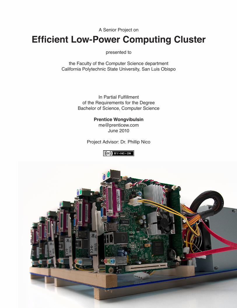
A Senior Project on
Efficient Low-Power Computing Clusterpresented to
the Faculty of the Computer Science departmentCalifornia Polytechnic State University, San Luis Obispo
In Partial Fulfillmentof the Requirements for the Degree
Bachelor of Science, Computer Science
Prentice [email protected]
June 2010
Project Advisor: Dr. Phillip Nico

ii
This work is licensed under the Creative Commons Attribution-Noncommercial-
Share Alike 3.0 United States License. To view a copy of this license, visit http://cre-
ativecommons.org/licenses/by-nc-sa/3.0/us/ or send a letter to Creative Commons,
171 Second Street, Suite 300, San Francisco, California, 94105, USA.
iii
Abstract
The purpose of this project is to demonstrate the idea that clustering together less
powerful but energy efficient machines that are commercially available can provide
more efficient computing. With a third of energy consumption in the United States
attributed to data centers, power efficiency has become an increasingly important
topic in computing. [1] Companies like Google have exceeded their grid’s capacities
and built datacenters next to hydroelectric dams to reduce power loss from trans-
mission and to increase their data center’s capacity. [2] These experiments aspire to
demonstrate a model for achieving a higher performance-per-watt in a larger scale
using commercially available low-power hardware.

iv
Acknowledgements
Thank you,
Dr. Phillip Nico, my Senior Project Advisor, for you advice and guidance
throughout the project.
Brian Oppenheim, my research partner, for motivating me and keeping me on
track. I value your a unique viewpoints and useful advice during the project.
Boon, Paul and Shannon, my family, for supporting me throughout my journey
through college.
v
Table of Contents
Abstract .................................................................................................................iii
Acknowledgements ............................................................................ iv
Background ..................................................................................................... 1
FAWN ................................................................................................................................... 1
(in)Efficiency of Fast Processors ...................................................................................... 1
Hadoop ................................................................................................................................. 2
MapReduce .......................................................................................................................... 2
System Description ............................................................................ 4
Low-Power COTS (x86) Considerations ........................................................................ 4
Mainboard ........................................................................................................................... 4
Power Supply ....................................................................................................................... 5
Storage Considerations ..................................................................................................... 5
Hardware List ..................................................................................................................... 6
System Design / Considerations ...................................................................................... 6
Optimizing Linux .............................................................................................................. 6
Node Management Software Design .............................................................................. 8
Waking up ........................................................................................................................... 9
vi
Implementation ...................................................................................... 10
Objective ............................................................................................................................ 10
Description ........................................................................................................................ 10
Overview of procedure .................................................................................................... 10
Quasi-Monte Carlo Computation ................................................................................. 10
Measuring Load Scaling Effectiveness ......................................................................... 11
Equipment Used ............................................................................................................... 12
Virtual Machine Server ................................................................................................... 12
Measurement Device ....................................................................................................... 12
Measuring “Off” Power Consumption ........................................................................ 12
Measuring Idle Power Consumption ........................................................................... 13
Measuring Power Consumption (under load) ............................................................ 13
Measurement Device Limitations ................................................................................. 14
LoadMon Server Implementation .................................................................................... 14
Hadoop Administrative Screens of Interest ............................................................... 15
Boot Time Optimization ................................................................................................ 16
Implementation Issues .................................................................................................... 17
Disabling components in BIOS ..................................................................................... 19
Data Collected ..........................................................................................20
Instantaneous Data ..........................................................................................................20
Power Consumption Data (Low-Power Cluster, No Power Scaling) ......................20
Power Consumption Data (Low-Power Cluster, Power Scaling) ............................ 21
Power Consumption Data (High-Power Cluster, No Power Scaling) .................... 21
Power Consumption Data (55mins, Short Jobs - Low-Power Cluster, Power Scal-
ing) ....................................................................................................................................22
vii
Power Consumption Data (55mins, Short Jobs - Low-Power Cluster, No Scaling)
22
Analysis & Conclusion ...............................................................24
Load Scale Algorithm Effectiveness .............................................................................25
Shortcomings in Node Hardware .................................................................................25
Comparison to Virtual Machine Cluster ....................................................................26
Bandwidth Concerns .......................................................................................................26
Storage Capacity ............................................................................................................... 27
Supporting Hardware ..................................................................................................... 27
Future Work ................................................................................................. 29
Software Improvements .................................................................................................. 29
Hardware Improvements ................................................................................................ 29
Power Supply Improvements ......................................................................................... 29
Varying Node Types ........................................................................................................ 29
Consolidate Power Supplies ...........................................................................................30
Bibliography ................................................................................................. 31
Appendix A: LoadMon ............................................................... 33
LoadMon.py ...................................................................................................................... 33
hosts.py ...............................................................................................................................38
pmcmd.py ..........................................................................................................................38
viii
Appendix B: hadoop-ctrl (rc.d script) ............40
hadoop-ctrl ........................................................................................................................40
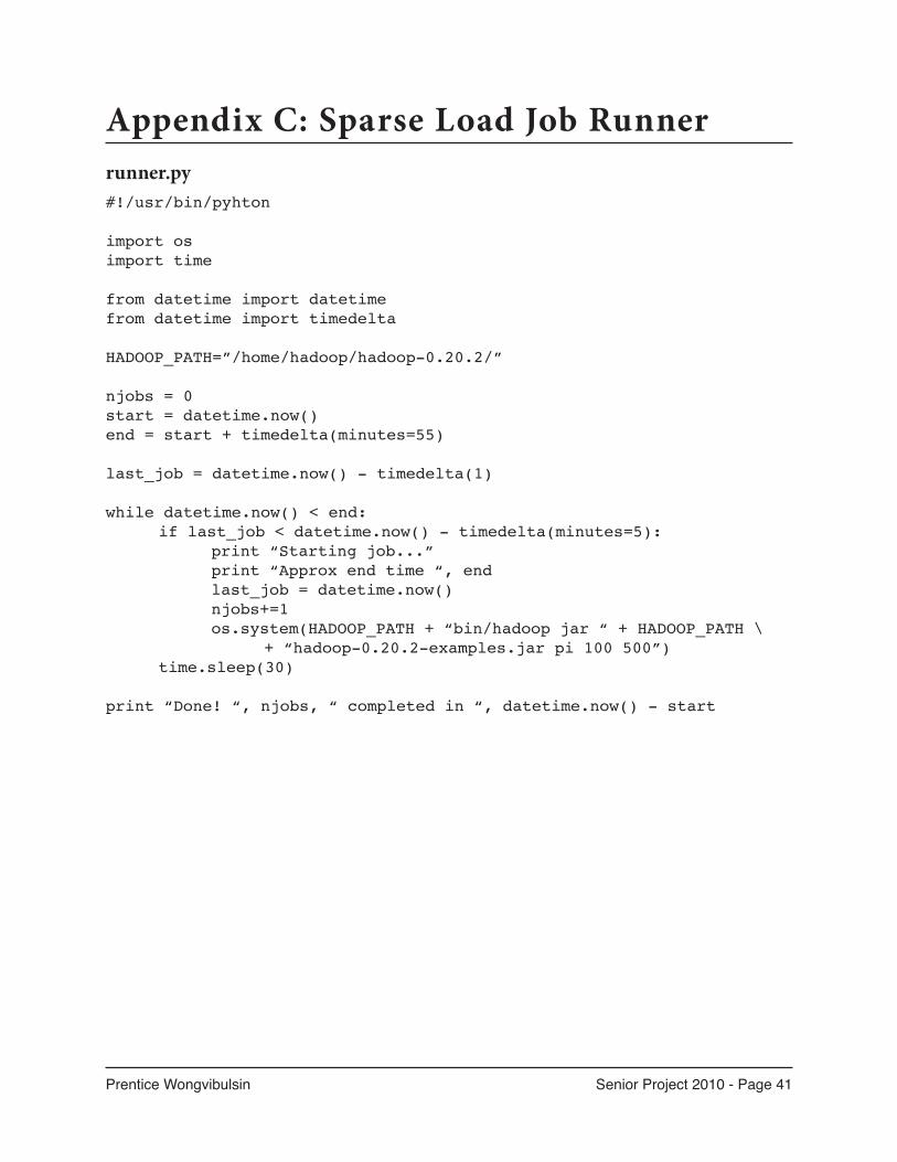
Appendix C: Sparse Load Job Runner ............. 41
runner.py ........................................................................................................................... 41
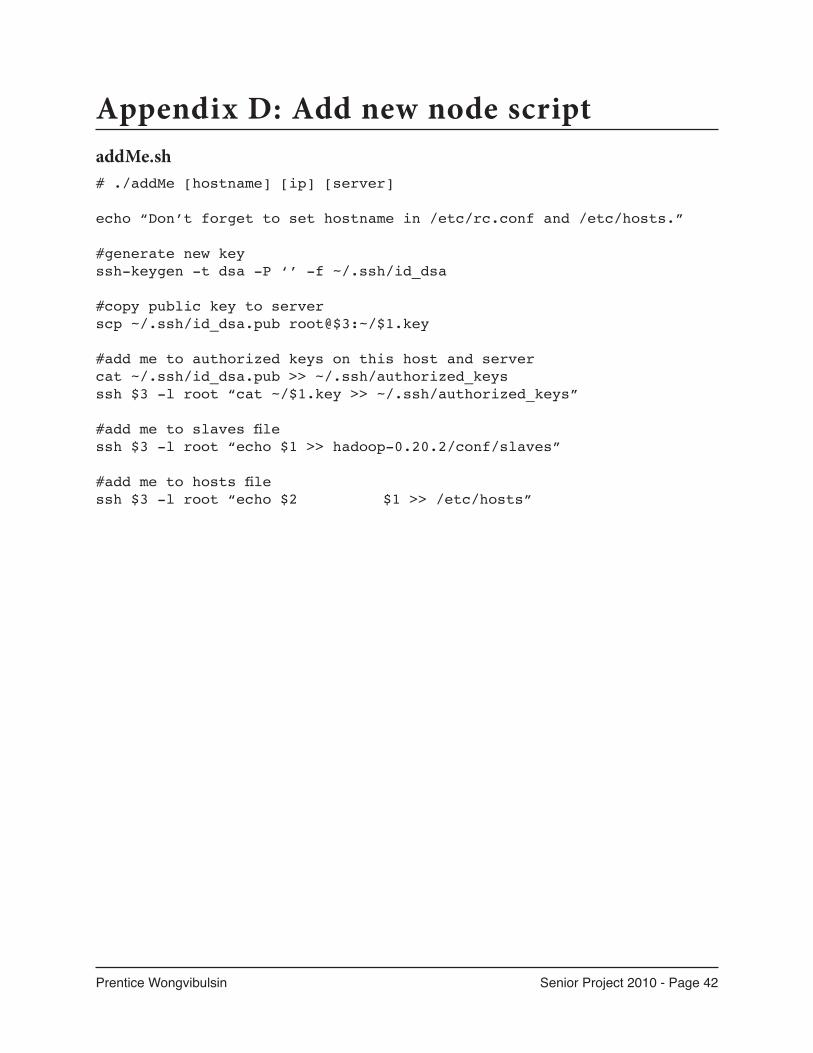
Appendix D: Add new node script .........................42
addMe.sh ............................................................................................................................42
Prentice Wongvibulsin Senior Project 2010 - Page 1
FAWN
Fast Array of Wimpy Nodes (FAWN)
is an energy efficient cluster project.
Their project runs embedded AMD
Geode processors with a datastore and
distributed computing architecture
they developed in-house. Each node in
their cluster consumes less than 4 watts
while being capable of performing over
1300 queries per second. [1]
(in)Efficiency of Fast Processors
As processors break records in clock
speed, power consumption grows at a
linearly proportional rate due to the
rapidly increasing transistor count and
cache sizes. [3]
Unfortunately, a lot of the extra power
consumed is wasted on the trade-offs
that are introduced in high-perfor-
mance computing such as out-of-order
execution and predictive branching.
[1] Intel and AMD have recently intro-
duced commercially available x86 chips
that consumes very little energy.
This research focuses on the Intel Atom
processor. The Atom processor has a
TDP (Thermal Design Power) of 2-4W
compared to a traditional server chip
such as an Intel Xeon processor which
has a TDP of 105W. [4] While the TDP
is not the maximum power the proces-
sor can dissipate, it is unlikely that the
processor will reach maximum power
dissipation under normal operating
conditions. [5] Thus, these low-power
processors consume only a fraction of
what high-end server hardware would.
In Vasudevan’s, et al. research, they
found that while a Xeon processor
could perform nearly 100,000 instruc-
tions per second. However, it did take
substantially more power to complete
that computation than the Atom pro-
cessor which is capable of a little over
1,000 instructions per second. When
Background
Prentice Wongvibulsin Senior Project 2010 - Page 2
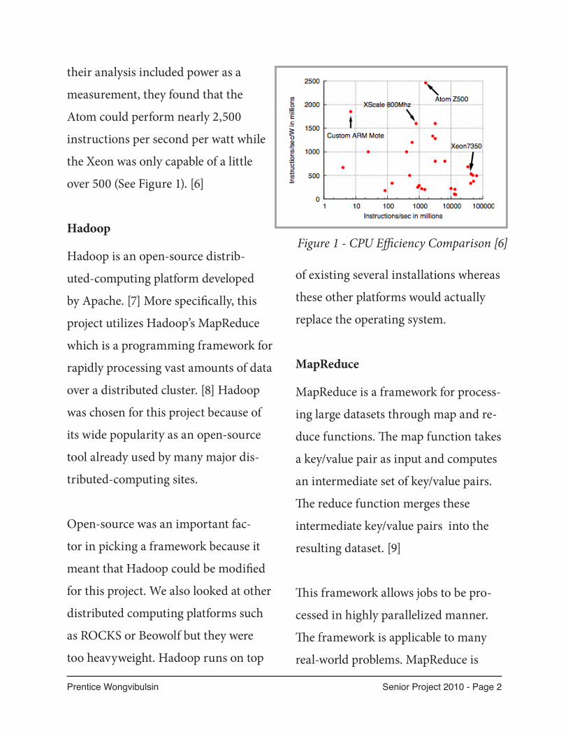
their analysis included power as a
measurement, they found that the
Atom could perform nearly 2,500
instructions per second per watt while
the Xeon was only capable of a little
over 500 (See Figure 1). [6]
Hadoop
Hadoop is an open-source distrib-
uted-computing platform developed
by Apache. [7] More specifically, this
project utilizes Hadoop’s MapReduce
which is a programming framework for
rapidly processing vast amounts of data
over a distributed cluster. [8] Hadoop
was chosen for this project because of
its wide popularity as an open-source
tool already used by many major dis-
tributed-computing sites.
Open-source was an important fac-
tor in picking a framework because it
meant that Hadoop could be modified
for this project. We also looked at other
distributed computing platforms such
as ROCKS or Beowolf but they were
too heavyweight. Hadoop runs on top
of existing several installations whereas
these other platforms would actually
replace the operating system.
MapReduce
MapReduce is a framework for process-
ing large datasets through map and re-
duce functions. The map function takes
a key/value pair as input and computes
an intermediate set of key/value pairs.
The reduce function merges these
intermediate key/value pairs into the
resulting dataset. [9]
This framework allows jobs to be pro-
cessed in highly parallelized manner.
The framework is applicable to many
real-world problems. MapReduce is
Figure 1 - CPU Efficiency Comparison [6]

Prentice Wongvibulsin Senior Project 2010 - Page 3
designed for complex jobs to be distrib-
uted across a large cluster of commod-
ity machines. [9]

Prentice Wongvibulsin Senior Project 2010 - Page 4
Low-Power COTS (x86)
Considerations
While this is largely a software imple-
mentation, it is important to select the
correct hardware for the project. All
our efforts could go towards reducing
power consumption in soft-
ware but it would have been a
moot effort with inefficient
hardware. [10] Google
uses the concept of “en-
ergy proportionality,”
meaning that hardware
should consume energy propor-
tional to its load.
Further, Google uses a metric called
Power Usage Effectiveness (PUE) to de-
termine the efficiency of their datacen-
ters. [11] Although it is not within the
scope of this project to make hardware
modifications to mitigate unnecessary
or excessive power consumption, these
concepts emphasize that the first step
to an efficient system is having the right
hardware.
Mainboard
There are a variety of low-power x86
boards available. Each of these main-
boards are sold with the processors
embedded with the
board unlike tradition-
al mainboards where
the processor can be
independently selected.
Considerations for purchas-
ing hardware included:
Cost (college student budget!)•
Flavor of Atom Processor•
Gigabit networking•
SATA port•
Minimal graphics, etc.•
Cost played a major deciding role in
component selection which greatly lim-
System Description

Prentice Wongvibulsin Senior Project 2010 - Page 5
ited the options. After researching and
comparing features of various boards,
the Intel D945GCLF2D mainboard
(pictured on previous page) featuring
an embedded Dual-Core Intel Atom
processor was chosen for this project.
Power Supply
Any part of the system can become a
bottleneck for optimizing efficiency.
According to Google’s research, the
average personal computer wastes
between 30% and 40% of the energy it
consumes due to an inefficient power
supply. [12] The power supply is a key
part of any system yet it is often
overlooked and selected as an
afterthought.
We choose a power sup-
ply based on the follow-
ing characteristics:
Cost (college student budget!)•
Active PFC feature•
High efficiency rating (80 Plus Cer-•
tification)
Given cost as a key factor once again,
the Rosewill RV300 (pictured below)
was chosen.
Storage Considerations
Traditional magnetic hard drives con-
sume a substantial amount of power.
For this project, compact flash (CF)
storage (solid state storage) was used to
reduce the power demand for storage
in the cluster. [13] compact flash cards
typically consume 30-60mA (100mA
maximum [14]) versus hard drives con-
suming around 8A-13A. [15]
Compact flash media is typi-
cally found in digital
cameras and other
portable devices so
an adapter was need-
ed. A 50-pin compact
flash to SATA (Serial
ATA) adaptor was used.
CF storage devices con-
forms to ATA specifications
so while running in IDE mode. The
disk appears as any other hard drive

Prentice Wongvibulsin Senior Project 2010 - Page 6
would to the system. [16]
Hardware List
Each node in this cluster (pictured be-
low) consists of the following hardware:
Intel D945GCLF2D Mainboard w/ •
embedded Intel Atom 330 (dual core
1.6Ghz) processor.
1 GB Crucial Rendition RAM•
Roswill ValueSeries RV300 Power •
Supply (300W)
Kingston 4GB Compact Flash •
Memory
SYBA SD-ADA40001 SATA II to •
Compact Flash Adapter (Marvell
88SA8052 Chipset)
System Design / Considerations
The cluster runs Hadoop on ArchLinux
2009.08. Using low-power hardware
should inherently reduce a substantial
amount power consumption in itself.
However, this project hopes to demon-
strate that software can further opti-
mize power consumption. Assuming
the cluster will not be running at 100%
capacity 24/7, turning off nodes which
are not in use will greatly cut down
power consumption.
Optimizing Linux
When turning nodes on and off, it is
essential to have each node boot up
very quickly to reduce overhead. This
requirement prompted the
selection of ArchLinux
(Arch) as the
Linux dis-
tribution
of choice.
ArchLinux
is a very
lightweight
distribu-
Prentice Wongvibulsin Senior Project 2010 - Page 7
tion highlighting a very minimal, bare-
bones install of Linux. [17]
Regardless of its lightweight nature,
Arch sports a very robust package
manager known as pacman. When set-
ting up the cluster, the very minimal
packages required for supporting Ha-
doop were installed.
The following packages were installed
via pacman:
openssh •
jdk (java6) •
rsync•
python (server node only)•
Because LoadMon is written in Python,
it was necessary to install Python on
the server node.
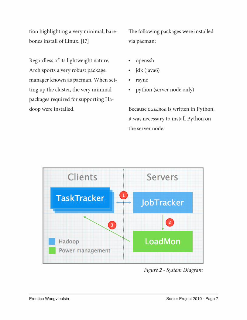
Figure 2 - System Diagram
Prentice Wongvibulsin Senior Project 2010 - Page 8
For testing, the following packages
were also installed:
mercurial - for version control •
vim - for text editing.•
A minimal selection of packages was
not only essential to maintain high
node performance but also due to
the limited amount of storage on the
nodes, a limitation from the use of
compact flash cards.
Additionally, the IPv6 module was
disabled to prevent complications since
Hadoop does not currently support
IPv6. [18]
Node Management Software Design
The power management software,
LoadMon, was designed as an indepen-
dent module. Managing the Hadoop
nodes did not requiring any modifi-
cation to Hadoop itself. This separa-
tion between the power management
software and the distributed comput-
ing framework demonstrates that this
power management scheme is not
specific to Hadoop and it is applicable
to other distributed computing clusters.
The diagram (figure 2, see previous
page) illustrates how the load monitor-
ing application hooks in to the Hadoop
system.
The blue modules represent the (un-
modified) Hadoop daemons and the
green represents the power manage-
ment additions to the cluster. The
numbered arrows represent dataflow
between the daemons. The paths are
described below and referenced paren-
thetically.
The Hadoop client daemons respon-
sible for performing the computations
(map/reduce tasks) are known as Task-
Trackers. The number of TaskTrackers
running will be scaled by the cluster’s
load. A JobTracker is the Hadoop dae-
mon that monitors the TaskTrackers
and distributes work (1). This daemon
is queried for node utilization data that
is used to decide which nodes to shut-
Prentice Wongvibulsin Senior Project 2010 - Page 9
down or wake up. Lastly, LoadMon is the
addition which is responsible for gath-
ering data from the JobTracker (2) and
issuing shutdown or wake commands
to client nodes (3).
Waking up
Wake-on-LAN (WOL), also known as
Magic Packet technology, was devel-
oped as part of the green PC initiative.
It is now widely supported in nearly all
network adaptors today. [19]
There are certainly more robust meth-
ods of waking client nodes than using
Wake-on-LAN (WOL). WOL does not
provide a reliable closed loop imple-
mentation for confirming that a cli-
ent is waking. Additionally, the WOL
implementation requires knowledge of
the target’s MAC address. Regardless, it
is sufficient for this project with certain
precautions.
Several restrictions are implemented
in our cluster to overcome this uncer-
tainty. All nodes must have a static IP
so there can be association between
hostname/IP and MAC address. More-
over, all nodes report their status using
an rd.d deamon. When the client node
finishes booting, it tells LoadMon that it
is ready to receive jobs. When the client
node is shutting down, it tells LoadMon
that it is being shutdown. Thus, in the
case where LoadMon issues a wake com-
mand and for whatever reason the tar-
get client never executed the command,
a timeout would occur and LoadMon
would know to reissue the command.
Designing a “daughter board” type in-
terface for each node would have been
a better solution for keeping track of of-
fline nodes; however, given the limited
time and scope of this project -- it was
unfeasible to engineer such a solution.
Prentice Wongvibulsin Senior Project 2010 - Page 10
Objective
To determine if substantial power sav-
ings is achievable by scaling the size
of the cluster based on analysis of the
cluster’s workload.
Description
The workload for this experiment is a
Map-reduce program that estimates
the value of Pi using quasi-Monte Carlo
method. This workload is run on the
cluster as power consumption is mea-
sured and time to completion is re-
corded. The experiment shall be run in
3 different configurations:
Atom cluster with no power man-•
agement
Atom cluster with power scaling•
AMD Opteron virtual cluster•
Overview of procedure
Measure power consumption idle.1.
Measure power consumption while 2.
under load.
Perform MapReduce job while 3.
measuring power consumption and
time to completion.
Perform multiple small MapReduce 4.
jobs spaced out over a fixed amount
of time while measuring power con-
sumption.
Quasi-Monte Carlo Computation
The estimation of pi is included as an
example application in the Hadoop
distribution. The algorithm takes two
parameters numMaps and numPoints.
To obtain a reasonable running time
on the cluster, 5,000 maps and 5,000
points were used. The following com-
mand is executed:
bin/hadoop jar hadoop-0.20.2-ex-
amples.jar pi 5000 5000
Implementation
Prentice Wongvibulsin Senior Project 2010 - Page 11
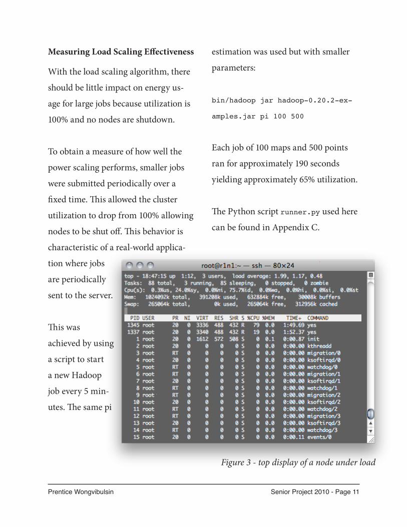
Measuring Load Scaling Effectiveness
With the load scaling algorithm, there
should be little impact on energy us-
age for large jobs because utilization is
100% and no nodes are shutdown.
To obtain a measure of how well the
power scaling performs, smaller jobs
were submitted periodically over a
fixed time. This allowed the cluster
utilization to drop from 100% allowing
nodes to be shut off. This behavior is
characteristic of a real-world applica-
tion where jobs
are periodically
sent to the server.
This was
achieved by using
a script to start
a new Hadoop
job every 5 min-
utes. The same pi
estimation was used but with smaller
parameters:
bin/hadoop jar hadoop-0.20.2-ex-
amples.jar pi 100 500
Each job of 100 maps and 500 points
ran for approximately 190 seconds
yielding approximately 65% utilization.
The Python script runner.py used here
can be found in Appendix C.
Figure 3 - top display of a node under load

Prentice Wongvibulsin Senior Project 2010 - Page 12
Equipment Used
The following pieces of hardware were
used in the experiment:
Low-power cluster hardware (de-•
scribed in previous section)
Netgear ProSafe 8 Port Gigabit •
Switch GS108
Virtual Machine Server (described •
below)
P3 Kill-A-Watt Power Meter P4400•
Virtual Machine Server
The virtual machine (VM) server is
used as a benchmark or compari-
son to give an idea of how the
low-power system performs.
The VM server has an AMD
Opteron 64-bit Dual Core
1.8Ghz processor and 4 GB
of RAM running Xen on
Ubuntu.
The virtual cluster
consists of 5 nodes to
match the low-power
cluster’s node count.
Measurement Device
Power measurements and energy con-
sumption data are collected with a
P3 Kill-A-Watt Power Meter P4400
(pictured below). The meter is rated
accurate within 0.2%. The meter is
capable of cumulative killowatt-hour
monitoring and instantaneous reading
of Watts. [20] It may not be the ideal
device for measuring power consump-
tion but it meets the budgetary require-
ments and it is sufficient to collect data
for this project.
Measuring “Off”
Power Consump-
tion
Three instantaneous
measurements were
taken. (1) Power con-
sumption of 1 node off,
(2) power consumption of
all nodes off, and (3) power
consumption of all nodes
turned off with switch on.

Prentice Wongvibulsin Senior Project 2010 - Page 13
Nodes are plugged into an outlet box
which is connected to the P3 power
meter.
Measuring Idle Power Consumption
To measure idle power, all nodes were
booted and left idle for 5 minutes. As
no fluctuations were observed in power
consumption, an instanta-
neous reading was taken and
recorded.
Measuring Power Consump-
tion (under load)
To measure power consump-
tion while under load, all cores
were made busy using the yes
command. Since these nodes are dual
core, two instances of the yes command
were run simultaneously to achieve
100% CPU utilization (see Figure 3).
Once no fluctuations were observed in
power consumption, an instantaneous
reading was taken.
Figure 4 (Above) - JobTracker
Administrative Screen
Figure 5 (Left) - JobTracker
Machine List
Prentice Wongvibulsin Senior Project 2010 - Page 14
Measurement Device Limitations
The Kill-A-Watt power meter is a con-
sumer product intended to estimate
power consumption and forecast elec-
tric bills. It was not designed for accu-
rate scientific measurements, etc. The
mode to measure power consumption
over time starts counting as soon as the
device is plugged in. There is no way to
reset the counter or pause data collec-
tion.
As a result, all measurements of power
consumption over time begin when
the nodes are turned on and the meter
begins recording. To obtain the power
consumed during a test, the current
power reading is recorded at the be-
ginning of the trial and then recorded
once again at the end giving us “start”
power and “end” power. The power
measurements obtained are:
Ptot = Pend - Pstart
Additionally, the unit of measurement
for power consumption over time is
KWH which doesn’t provide much
resolution. To obtain a better reading,
longer tests are conducted.
LoadMon Server Implementation
The goal of load scaling is to have the
number of online nodes on proportion-
al to the amount of work the cluster has
to perform. Determining the cluster’s
load is the first step to achieving this
goal.
Load is determined by extract-
ing data from Hadoop’s Job-
Tracker administrative screen.
The LoadMon process performs
an HTTP request for the Na-
meNode’s administrative screen
and parses the current load.
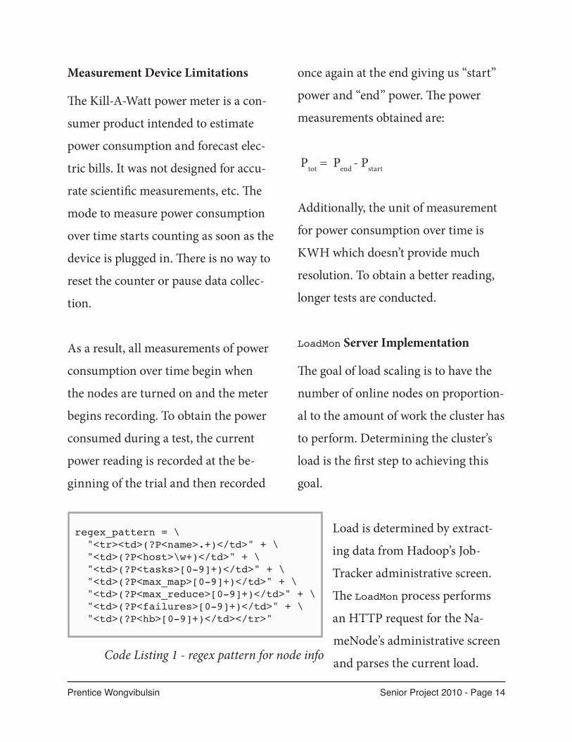
regex_pattern = \ "<tr><td>(?P<name>.+)</td>" + \ "<td>(?P<host>\w+)</td>" + \ "<td>(?P<tasks>[0-9]+)</td>" + \ "<td>(?P<max_map>[0-9]+)</td>" + \ "<td>(?P<max_reduce>[0-9]+)</td>" + \ "<td>(?P<failures>[0-9]+)</td>" + \ "<td>(?P<hb>[0-9]+)</td></tr>"
Code Listing 1 - regex pattern for node info
Prentice Wongvibulsin Senior Project 2010 - Page 15
Based on this data, the LoadMon deter-
mines if each node should be turned
on or off. If the cluster is running at or
near 100% capacity, LoadMon will acti-
vate additional nodes. However, if the
cluster is running below 50% capacity,
LoadMon will begin to shutdown nodes.
Hadoop Administrative Screens of
Interest
The screens of interest in Hadoop’s
JobTracker are the main
administrative screen (/
jobtracker.jsp) and the
machine list display (/ma-
chines.jsp?type=active).
The main administrative
screen displays the current
load and capacity of the
cluster (see Figure 4). The
raw data consists of:
Number of Maps being •
performed
Number of Reduces be-•
ing performed
Total Submissions•
Number of Nodes online•
Map Task Capacity•
Reduce Task Capacity•
Average Task per Node•
Blacklisted Nodes•
The specific fields of interest are the
number of maps, the number of reduc-
es, map capacity and reduce capacity.
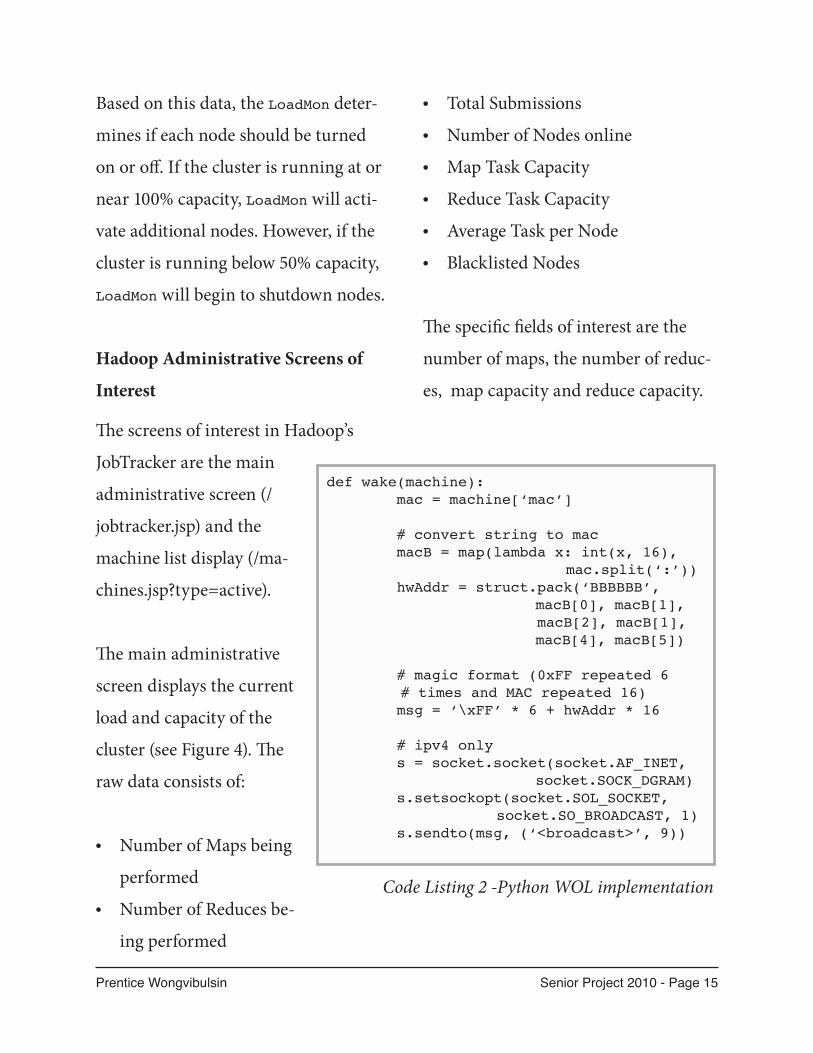
def wake(machine): mac = machine[‘mac’]
# convert string to mac macB = map(lambda x: int(x, 16), mac.split(‘:’)) hwAddr = struct.pack(‘BBBBBB’, macB[0], macB[1], macB[2], macB[1], macB[4], macB[5])
# magic format (0xFF repeated 6 # times and MAC repeated 16) msg = ‘\xFF’ * 6 + hwAddr * 16
# ipv4 only s = socket.socket(socket.AF_INET, socket.SOCK_DGRAM) s.setsockopt(socket.SOL_SOCKET, socket.SO_BROADCAST, 1) s.sendto(msg, (‘<broadcast>’, 9))
Code Listing 2 -Python WOL implementation
Prentice Wongvibulsin Senior Project 2010 - Page 16
The individual node display contains
the individual node’s load and capaci-
ties (see Figure 5).
The raw data consists of:
Node Name•
Hostname•
# running tasks•
Max Map Tasks•
Max Reduce Tasks•
Failures•
Seconds since last heartbeat•
The hostname, number of running
tasks and max tasks are the primary
interests of this study.
A Python regular expression (regex)
is used to extract this data from the
HTML provided by these screens.
In the Future Work section, better
methods for this implementation are
discussed. Code Listing 1 contains an
example of a regular expression used to
parse individual node statuses.
Boot Time Optimization
Since nodes will then be constantly
turned on and off, the boot and shut-
down times for a node becomes very
important. As discussed earlier, the
Linux distribution chosen has been op-
timized for quick power on and power
off to reduce any overhead waiting for
nodes to become ready. Average startup
time is 27.2 seconds. Average shutdown
time is 12.9 seconds.
Startup times generally can also be
reduced by disabling self-checks and
optimizing boot order in BIOS. Self-
check that run at boot are generally in-
tended for a consumer who would boot
their computer maybe once a day. The
slight impact in startup time is not very
noticeable; however, when our nodes
are being turned on and off every few
minutes or hours, not only is the im-
pact noticeable but the checks become
unnecessary because of how often they
are run.
Prentice Wongvibulsin Senior Project 2010 - Page 17
The shutdown command is issued to
a remote node via SSH. As part of the
Hadoop installation procedure, all
nodes share DSA keypairs allowing
LoadMon to piggyback off this require-
ment. Wake commands are issued
using WOL. Problems with WOL and
our solution for overcoming those is-
sues have been previously discussed
in the System Description section of
this document. Simply, the client is
responsible for calling home when that
node is ready to receive a job. If a call-
home is not received before a specified
timeout value, the node is reissued a
wake command until it does wake, or a
maximum number of retries is reached
(at which point the node shall be con-
sidered dead).
Wake-On-Lan/Magic Packet Imple-
mentation
A magic packet is defined as 0xFF re-
peated 6 times followed by the target’s
MAC address repeated 16 times. [19]
A Python implementation of this Mag-
ic Packet used in this project is shown
in Code Listing 2. It accepts a “ma-
chine” entry which is a dict type con-
taining ‘name’ for hostname and ‘mac’
for MAC address formatted as a string.
The individual octets from the MAC
address string is converted and packed.
The raw mac address is then repeated
16 times preceded by 0xFFFFFF as
specified by the Magic Packet format.
Complete implementation of shutdown
and wake commands can be found in
pmcmd.py (see Appendix A).
Complete specification machine data
can be found in hosts.py (see Appen-
dix A).
Implementation Issues
Potentially, a wake command could be
issued right after a node has been is-
sued a shutdown command but before
Prentice Wongvibulsin Senior Project 2010 - Page 18
it has completely turned off (before the
NameNode discovers that the client is
offline).
This issue is not addressed in our soft-
ware because the job will simply time
out when the node stops sending heart-
beats and the job will be reassigned to a
new node. While this may seem rather
inefficient, with the policy of shutting
down nodes only when running at 50%
capacity, it is rather unlikely that this
condition will occur. Further, with the
low timeout values, it should not cause
much degradation in performance.
Thus, while this implementation re-
quires no modifications to Hadoop, it
does require certain configuration of
Hadoop.
Firstly, nodes may leave and join a run-
ning Hadoop cluster; however, it was
not designed to have nodes constantly
turning on and off. As a result, the
default timeout is rather high causing
offline nodes to remain as a ghost for
up to 10 minutes (60,000 milliseconds)
after the last heartbeat is received. This
implementation requires that number
to be lowered so that offline nodes are
not allocated for jobs. The configura-
tion mapred.tasktracker.expiry.in-
terval allows us to specify the interval
(in milliseconds).
When lowering the timeout value, it
is important to select a number that is
not too low. In the experiments, set-
ting it to 6 seconds (6,000 milliseconds)
caused numerous jobs to fail. When
a node is under load, the heartbeat is
sometimes delayed. In the case where
the heartbeat takes longer than time
timeout value, the task is killed by the
JobTracker. The value of 30 seconds
(30,000 milliseconds) worked well for
this experiment.
Secondly, this implementation depends
on the formatting of the Hadoop ad-
ministrative web interface. It is possible
to modify Hadoop to include a dis-
play that is formatted for our daemon;
Prentice Wongvibulsin Senior Project 2010 - Page 19
however, to refrain from modifying
Hadoop it was not implemented. The
future work section discusses possible
implementations.
Disabling components in BIOS
All non-essential devices are disabled
in BIOS. This includes the serial port,
parallel port, audio, and USB. Unfor-
tunately these changes did not demon-
strate any apparent power savings.
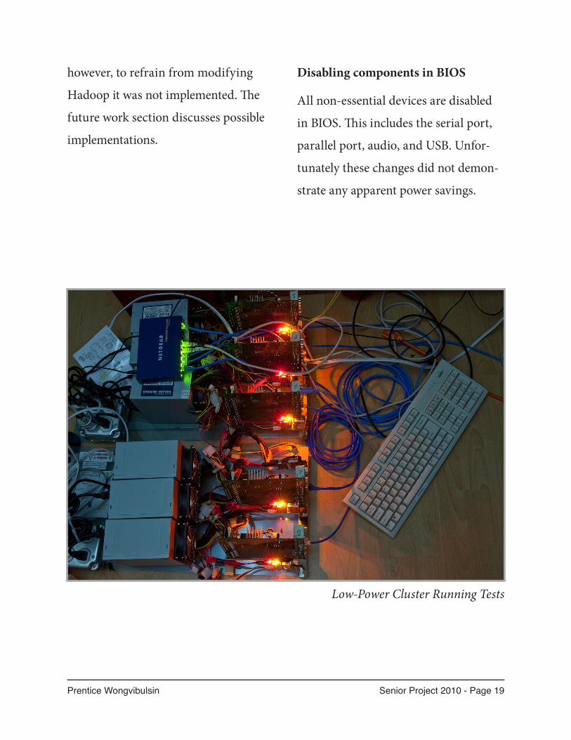
Low-Power Cluster Running Tests
Prentice Wongvibulsin Senior Project 2010 - Page 20
Instantaneous Data
An offline node consumes:
3W
One online node (idle/load):
33W / 35W
Five nodes offline (idle):
24W
Five nodes online (idle / load):
220W / 250W
Five nodes load-scaled (idle - 1 online):
60W
VM Cluster (idle / load):
144W / 184W
Power Consumption Data (Low-Pow-
er Cluster, No Power Scaling)
Average Runtime: 55mins, 1sec
Average Energy Usage: 0.22 KWH
Trial #1
Start Time: 17:02:58
End Time: 17:57:14
Runtime: 54mins, 16sec
Start Meter Reading: 7.60 KWH
End Meter Reading: 7.82 KWH
Energy Usage: 0.22 KWH
Trail #2
Start Time: 18:07:43
End Time: 19:02:37
Runtime: 54mins, 53sec
Start Meter Reading: 7.84 WKH
End Meter Reading: 8.07 KWH
Energy Usage: 0.23 KWH
Trial #3
Start Time: 19:26:32
End Time: 20:21:43
Runtime: 55mins, 11sec
Start Meter Reading: 8.13 KWH
End Meter Reading: 8.35 KWH
Energy Usage: 0.22 KWH
Data Collected
Prentice Wongvibulsin Senior Project 2010 - Page 21
Power Consumption Data (Low-Pow-
er Cluster, Power Scaling)
Average Runtime: 1hrs, 2mins, 58sec
Average Energy Consumed: 0.22 KWH
Trial #1
Start Time: 17:03:44
End Time: 18:05:21
Runtime: 1hrs, 1mins, 37sec
Start Meter Reading: 1.15 KWH
End Meter Reading: 1.37 KWH
Energy Usage: 0.22 KWH
Trial #2
Start Time: 18:11:37
End Time: 19:15:57
Runtime: 1hrs, 4mins, 20sec
Start Meter Reading: 1.39 KWH
End Meter Reading: 1.61 KWH
Energy Usage: 0.22 KWH
Power Consumption Data (High-Pow-
er Cluster, No Power Scaling)
Average Runtime: 1hrs, 33mins, 10sec
Average Energy Consumed: 0.30 KWH
Trial #1
Start Time: 03:38:03
End Time: 05:08:50
Runtime: 1hrs, 30mins, 47sec
Start Meter Reading: 0.01 KWH
End Meter Reading: 0.31 KWH
Energy Usage: 0.30 KWH
Trial #2
Start Time: 05:23:55
End Time: 06:57:17
Runtime: 1hrs, 33mins, 21sec
Start Meter Reading: 0.34 KWH
End Meter Reading: 0.63 KWH
Energy Usage: 0.29 KWH
Trial #3
Start Time: 07:22:35
End Time: 08:57:59
Runtime: 1 hrs, 35mins, 23sec
Start Meter Reading: 0.68 KWH
End Meter Reading: 0.98 KWH
Energy Usage: 0.30 KWH

Prentice Wongvibulsin Senior Project 2010 - Page 22
Power Consumption Data (55mins,
Short Jobs - Low-Power Cluster, Pow-
er Scaling)
Average Energy Consumed: 0.13 KWH
Trial #1
Jobs Completed: 11
Actual Runtime: 58mins
Start Meter Reading: 0.86 KWH
End Meter Reading: 0.99 KWH
Energy Usage: 0.13 KWH
Trail #2
Jobs Completed: 11
Actual Runtime: 57mins
Start Meter Reading: 1.01 KWH
End Meter Reading: 1.14 KWH
Energy Usage: 0.13 KWH
Trail #3
Jobs Completed: 11
Actual Runtime: 57mins
Start Meter Reading: 1.16 KWH
End Meter Reading: 1.29 KWH
Energy Usage: 0.13 KWH
Power Consumption Data (55mins,
Short Jobs - Low-Power Cluster, No
Scaling)
Average Energy Consumed: 0.22 KWH
Jobs Completed: 11
Actual Runtime: 56mins
Start Meter Reading: 1.23 KWH
End Meter Reading: 1.45 KWH
Energy Usage: 0.22 KWH
Prentice Wongvibulsin Senior Project 2010 - Page 23
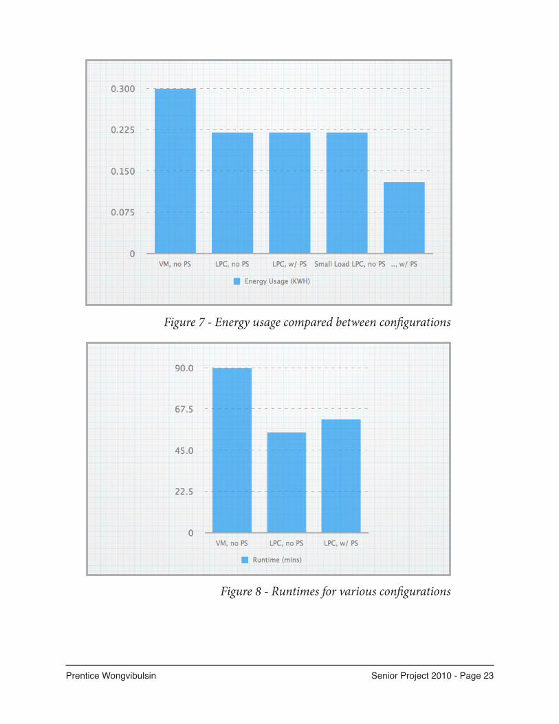
Figure 7 - Energy usage compared between configurations
Figure 8 - Runtimes for various configurations
Prentice Wongvibulsin Senior Project 2010 - Page 24
This experiment demonstrates shutting
down idle nodes in a sparsely utilized
cluster will yield substantial energy
savings.
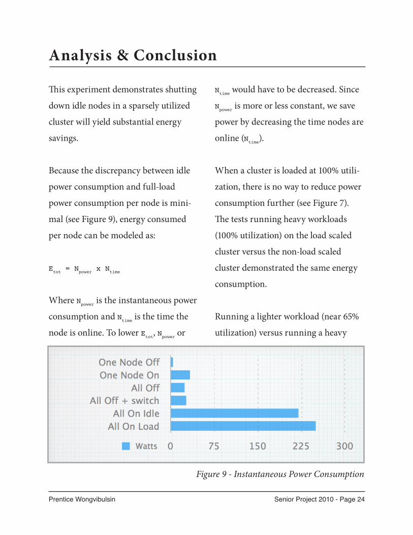
Because the discrepancy between idle
power consumption and full-load
power consumption per node is mini-
mal (see Figure 9), energy consumed
per node can be modeled as:
Etot = Npower x Ntime
Where Npower is the instantaneous power
consumption and Ntime is the time the
node is online. To lower Etot, Npower or
Ntime would have to be decreased. Since
Npower is more or less constant, we save
power by decreasing the time nodes are
online (Ntime).
When a cluster is loaded at 100% utili-
zation, there is no way to reduce power
consumption further (see Figure 7).
The tests running heavy workloads
(100% utilization) on the load scaled
cluster versus the non-load scaled
cluster demonstrated the same energy
consumption.
Running a lighter workload (near 65%
utilization) versus running a heavy
Analysis & Conclusion
Figure 9 - Instantaneous Power Consumption
Prentice Wongvibulsin Senior Project 2010 - Page 25
workload (100% utilization) also dem-
onstrates the same energy consumption
on a non-load scaled cluster because
Npower is the same when idle or under
load.
Load Scale Algorithm Effectiveness
For heavy-workload tests on the low-
power cluster with and without the
power scaling algorithm, runtimes
were on par. The power-scaled cluster
configuration took slightly longer on
average because when the job is initial-
ly submitted, the load is at 0% and only
1 node is online. It takes approximately
2-3 minutes for the remaining nodes to
wake up after the job is submitted. This
delay results in a slightly longer run-
time (see Figure 7). The delay is con-
stant, and does not vary for different
job sizes because it only occurs during
job startup.
The energy consumed for 65% utiliza-
tion in the load scaled cluster yielded
a substantial savings when compared
to the non-load scaled cluster. The
low-power cluster used 0.22 KWH of
energy during 100% utilization tri-
als. Ideally, if 65% of the work is being
done, the cluster ought to consume 0.14
KWH (65% of 0.22 KWH). The cluster
actually consumed 0.13 KWH which is
close! This implementation would not
be able to reach that ideal condition be-
cause one node must always stay online
to accept jobs even when no work is
being done.
Shortcomings in Node Hardware
Based on observations in this project,
current commercial off the shelf hard-
ware is not the ideal platform for de-
veloping an energy efficient computing
cluster. The processor’s TDP is 4W but
the supporting chipset draws a sub-
stantially greater amount of electricity.
These boards are designed with the av-
erage home user in mind. They are de-
signed for watching movies and surfing
the web. Thus, most of the components
on the board are unnecessary for our
computations (audio chipset, graphics
processing unit, etc.).

Prentice Wongvibulsin Senior Project 2010 - Page 26
Manufactures must begin to see the
market for these boards to be used as
home fileservers for storing data, video
and music. These boards could be
stripped of the components for playing
back audio and decoding video, hope-
fully reducing their power consump-
tion.
Comparison to Virtual Machine Clus-
ter
Despite the apparently disappointing
numbers from our hardware, it was
interesting to find that the low-power
cluster had a better performance per
watt than the server-class hardware.
Bandwidth Concerns
An individual node in the average
Hadoop cluster may process around
100 MB/sec of data. [21] Our nodes
are equipped with gigabit ethernet
and should have no problems transfer-
ring data at gigabit speeds; however, a
system can only go as fast as its slow-
est component. The average sequen-
tial read speed of the Compact Flash
(CF) media used in this cluster is 21.5
MB/sec. The performance of this card
is fairly poor even when compared
to even a consumer hard drive. The
Western Digital 320 GB 7200 RPM
averages 75.4 MB/sec and a RAID 5 of
5 Western Digital 500 GB 7200 RPM
drives averages 130.4 MB/sec. High-
end servers generally have disks that
will perform substantially better than
this hardware. Moreover, the media we
used in our experiments would have
caused a bottleneck for most applica-
tions of a Hadoop cluster.
The challenge can easily be overcome
by using high-end solid state drives
(SSDs) or faster Compact Flash cards.
High end solid state drives have se-
quential read speeds up to 250 MB/s
while maintaining relatively low power
consumption. [22]
Note: Sequential read bandwidth for
the Compact Flash drive, Western
Digital 320 GB drive and the RAID 5
Prentice Wongvibulsin Senior Project 2010 - Page 27
were gathered using hdparm utility.
The following command was executed:
hdparm -t (drive)
The command was executed three
times on each drive while there was
little to no I/O activity and then the
results were averaged.
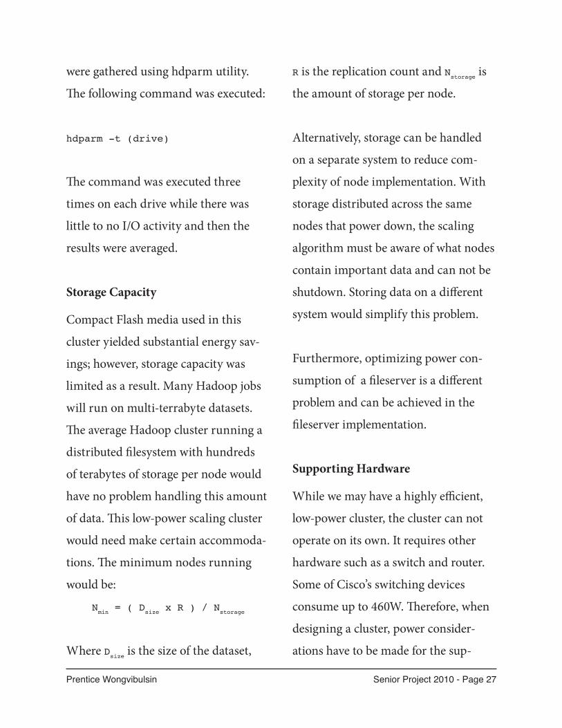
Storage Capacity
Compact Flash media used in this
cluster yielded substantial energy sav-
ings; however, storage capacity was
limited as a result. Many Hadoop jobs
will run on multi-terrabyte datasets.
The average Hadoop cluster running a
distributed filesystem with hundreds
of terabytes of storage per node would
have no problem handling this amount
of data. This low-power scaling cluster
would need make certain accommoda-
tions. The minimum nodes running
would be:
Nmin = ( Dsize x R ) / Nstorage
Where Dsize is the size of the dataset,
R is the replication count and Nstorage is
the amount of storage per node.
Alternatively, storage can be handled
on a separate system to reduce com-
plexity of node implementation. With
storage distributed across the same
nodes that power down, the scaling
algorithm must be aware of what nodes
contain important data and can not be
shutdown. Storing data on a different
system would simplify this problem.
Furthermore, optimizing power con-
sumption of a fileserver is a different
problem and can be achieved in the
fileserver implementation.
Supporting Hardware
While we may have a highly efficient,
low-power cluster, the cluster can not
operate on its own. It requires other
hardware such as a switch and router.
Some of Cisco’s switching devices
consume up to 460W. Therefore, when
designing a cluster, power consider-
ations have to be made for the sup-

Prentice Wongvibulsin Senior Project 2010 - Page 28
porting devices as well. In a large scale
application we may consider shutting
off sets of nodes which share the same
switch so that the switch can be pow-
ered down as well.
Prentice Wongvibulsin Senior Project 2010 - Page 29
Software Improvements
In a Hadoop implementation, a new
web interface could be developed for
LoadMon so the output would be opti-
mized for parsing. Hadoop’s web inter-
face uses Jetty which makes it easy to
develop new views for the data. [23]
Hardware Improvements
Each board consumes 4W even when
off. Developing a custom node manage-
ment solution that not only shuts down
the node but also cuts power to the
PSU will conserve even more power.
Using low-power microprocessors such
as the MSP430 Micro Control Unit
(MCU). These 3.6V MCUs operate with
as little as 0.7 μA with real-time clock
(RTC) and 200 μA active. That is less
than 1W! One of these MCUs can addi-
tionally control multiple boards yield-
ing additional power savings.
Power Supply Improvements
PSUs are very inefficient because they
must comply to specifications which
require multiple output voltages. In
their paper, Hoelzle and Weihl as-
sert that simplifying the power supply
design to only provide a single voltage
allows manufactures to produce more
efficient units. Google has implemented
this strategy in their own hardware and
have achieved over 90% efficiency. [12]
While Google’s implementation is not
available to the consumer, new pro-
grams are being developed to encour-
age manufactures to produce more
efficient power supplies. The 80Plus
program certifies PSUs that can per-
form at high efficiencies. [24]
Varying Node Types
Mixing low-power hardware with
server class hardware could balance
the shortcomings of low-power with
powerful processors. The load scaling
algorithms would have to be aware of
Future Work

Prentice Wongvibulsin Senior Project 2010 - Page 30
the various types of nodes and have a
weighted
Consolidate Power Supplies
Atom boards have a much lower power
requirement than traditional desktop
boards. It is then possible to run mul-
tiple Atom boards using a single power
supply.
Using a single power supply to power
multiple boards would reduce the
amount of power lost to the power sup-
ply’s inefficiency. Modifications to the
power supplies ATX protocols would be
required. Additionally, the load scaling
software could optimize online nodes
by attached power supply. For example,
if there are two power supplies online
and a node has to be shutdown, select
the node on the power supply with less
online nodes so the entire power supply
can be shut off.
Prentice Wongvibulsin Senior Project 2010 - Page 31
Bibliography
[1] Anderson, Franklin, Kaminsky, Phanishayee, Tan, Vasudevan. FAWN: A Fast
Array of Wimpy Nodes. In 2nd ACM Symposium on Operating Systems Prin-
ciples (SOPS’09). 2009.
[2] http://www.datacenterknowledge.com/archives/2007/01/20/google-planning-
two-huge-sc-facilities/
[3] Gunther, Binns, Carmean, Hall. Managing the Impact of Increasing Micropro-
cessor Power Consumption. Intel Technology Journal Q1. 2001
[4] http://www.intel.com/pressroom/kits/quickreffam.htm
[5] Intel® CoreTM Duo Processor and Intel® CoreTM Solo Processor on 65
nm Process Whitepaper 309221-006 http://www.intel.com/design/mobile/
datashts/309221.htm
[6] Vasudevan, Franklin, Anderson, Phanishayee, Tan, Kiminsky, Moraru. FAWN-
damentally Power-efficient Clusters. 2009
[7] http://hadoop.apache.org/
[8] http://hadoop.apache.org/mapreduce/
[9] Dean, Ghemawat. MapReduce: Simplified Data Processing on Large Clusters.
Google, Inc. 2004. http://labs.google.com/papers/mapreduce.html
[10] http://www.google.com/corporate/green/datacenters/step1.html

Prentice Wongvibulsin Senior Project 2010 - Page 32
[11] http://www.google.com/corporate/green/datacenters/measuring.html
[12] Hoelzle and Weihl. High-efficincy power supplies for home computers and
servers. Google Inc. 2006. http://research.google.com/pubs/pub32467.html
[13] http://www.intel.com/design/flash/nand/mainstream/index.htm
[14] http://www.compactflash.org/faqs/faq.php#power
[15] http://ixbtlabs.com/articles2/storage/hddpower.html
[16] http://www.compactflash.org/info/cfinfo.php
[17] http://www.archlinux.org/about/
[18] http://wiki.apache.org/hadoop/HadoopIPv6
[19] Magic Packet Technology White Paper #20213. AMD. 1995
[20] http://www.p3international.com/products/special/P4400/P4400-CE.html
[21] http://wiki.apache.org/hadoop/FAQ#A28
[22] http://www.intel.com/cd/channel/reseller/asmo-na/eng/products/nand/feature/
index.htm
[23] http://jetty.codehaus.org/jetty/
[24] http://www.80plus.org/
Prentice Wongvibulsin Senior Project 2010 - Page 33
Appendix A: LoadMonLoadMon.py#!/usr/bin/python# install me in crontab to run every minute:# * * * * * python LoadMon.py
import osimport urllibimport reimport timeimport hostsimport pmcmdimport loggingimport logging.handlersimport randomimport picklefrom datetime import datetimefrom datetime import timedelta
STATUS_FILENAME=’/var/log/LoadMon-status’
WAKING_FILENAME=’/var/log/LoadMon-wakeup’
LOG_FILENAME=’/var/log/LoadMon.log’
# Set up a specific logger with our desired output level
my_logger = logging.getLogger(‘LoadMon Log’)my_logger.setLevel(logging.DEBUG)
# Add the log message handler to the loggerhandler = logging.handlers.RotatingFileHandler( LOG_FILENAME, maxBytes=800000, backupCount=5)# create formatterformatter = logging.Formatter( \ “%(asctime)s - %(name)s - %(levelname)s - %(message)s”)# add formatter to chhandler.setFormatter(formatter)handler.setLevel(logging.DEBUG)
my_logger.addHandler(handler)
# returns a tuple of (hostname, tasks running, max map, max reduce)def nodeList(): node_status_html = urllib.urlopen( \

Prentice Wongvibulsin Senior Project 2010 - Page 34
‘http://localhost:50030/machines.jsp?type=active’).read() entry_repat = “<tr><td>(?P<name>.+)</td>” + \ “<td>(?P<host>\w+)</td>” + \ “<td>(?P<tasks>[0-9]+)</td>” + \ “<td>(?P<max_map>[0-9]+)</td>” + \ “<td>(?P<max_reduce>[0-9]+)</td>” + \ “<td>(?P<failures>[0-9]+)</td>” + \ “<td>(?P<hb>[0-9]+)</td></tr>” entry_regex = re.compile(entry_repat)
result = entry_regex.finditer(node_status_html) retval = map(lambda x: (x.group(‘host’), \ int(x.group(‘tasks’)), \ int(x.group(‘max_map’)), \ int(x.group(‘max_reduce’))), result)
retval_dict = {}
for entry in retval: retval_dict[entry[0]] = (entry[1], entry[2], entry[3])
return retval_dict
def clusterStatus(): cluster_status_html = urllib.urlopen( \ ‘http://localhost:50030/jobtracker.jsp’).read() stat_repat = r”<tr><td>(?P<maps>[0-9]+)</td>” + \ “<td>(?P<reduces>[0-9]+)</td>” + \ “<td>(?P<submit>[0-9]+)</td>” + \ “<td><a href=\”machines.jsp\?type=active\”>” + \ “(?P<nodes>[0-9]+)</a></td>” + \ “<td>(?P<map_max>[0-9]+)</td>” + \ “<td>(?P<reduce_max>[0-9]+)</td>” + \ “<td>(?P<avgtasknode>[\.0-9]+)</td>” + \ “<td><a href=\”machines.jsp\?type=blacklisted\”>” + \ “(?P<blacklist>[0-9]+)</a></td>” + \ “</tr>”
stat_regex = re.compile(stat_repat)
result = stat_regex.finditer(cluster_status_html) retval = map(lambda x: (int(x.group(‘maps’)), \ int(x.group(‘reduces’)), \ int(x.group(‘map_max’)), \ int(x.group(‘reduce_max’))), result)
return retval[0]
def main():
Prentice Wongvibulsin Senior Project 2010 - Page 35
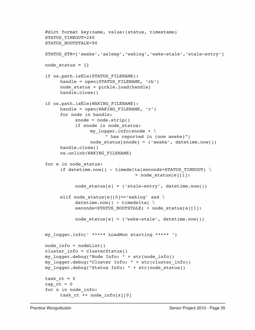
#dict format key:name, value:(status, timestame) STATUS_TIMEOUT=240 STATUS_BOOTSTALE=90
STATUS_STR=[‘awake’,’asleep’,’waking’,’wake-stale’,’stale-entry’]
node_status = {}
if os.path.isfile(STATUS_FILENAME): handle = open(STATUS_FILENAME, ‘rb’) node_status = pickle.load(handle) handle.close()
if os.path.isfile(WAKING_FILENAME): handle = open(WAKING_FILENAME, ‘r’) for node in handle: snode = node.strip() if snode in node_status: my_logger.info(snode + \ “ has reported in (now awake)”) node_status[snode] = (‘awake’, datetime.now()) handle.close() os.unlink(WAKING_FILENAME)
for e in node_status: if datetime.now() - timedelta(seconds=STATUS_TIMEOUT) \ > node_status[e][1]:
node_status[e] = (‘stale-entry’, datetime.now())
elif node_status[e][0]==’waking’ and \ datetime.now() - timedelta( \ seconds=STATUS_BOOTSTALE) > node_status[e][1]:
node_status[e] = (‘wake-stale’, datetime.now())
my_logger.info(‘ ***** LoadMon starting ***** ‘)
node_info = nodeList() cluster_info = clusterStatus() my_logger.debug(“Node Info: “ + str(node_info)) my_logger.debug(“Cluster Info: “ + str(cluster_info)) my_logger.debug(“Status Info: “ + str(node_status))
task_ct = 0 cap_ct = 0 for x in node_info: task_ct += node_info[x][0]
Prentice Wongvibulsin Senior Project 2010 - Page 36
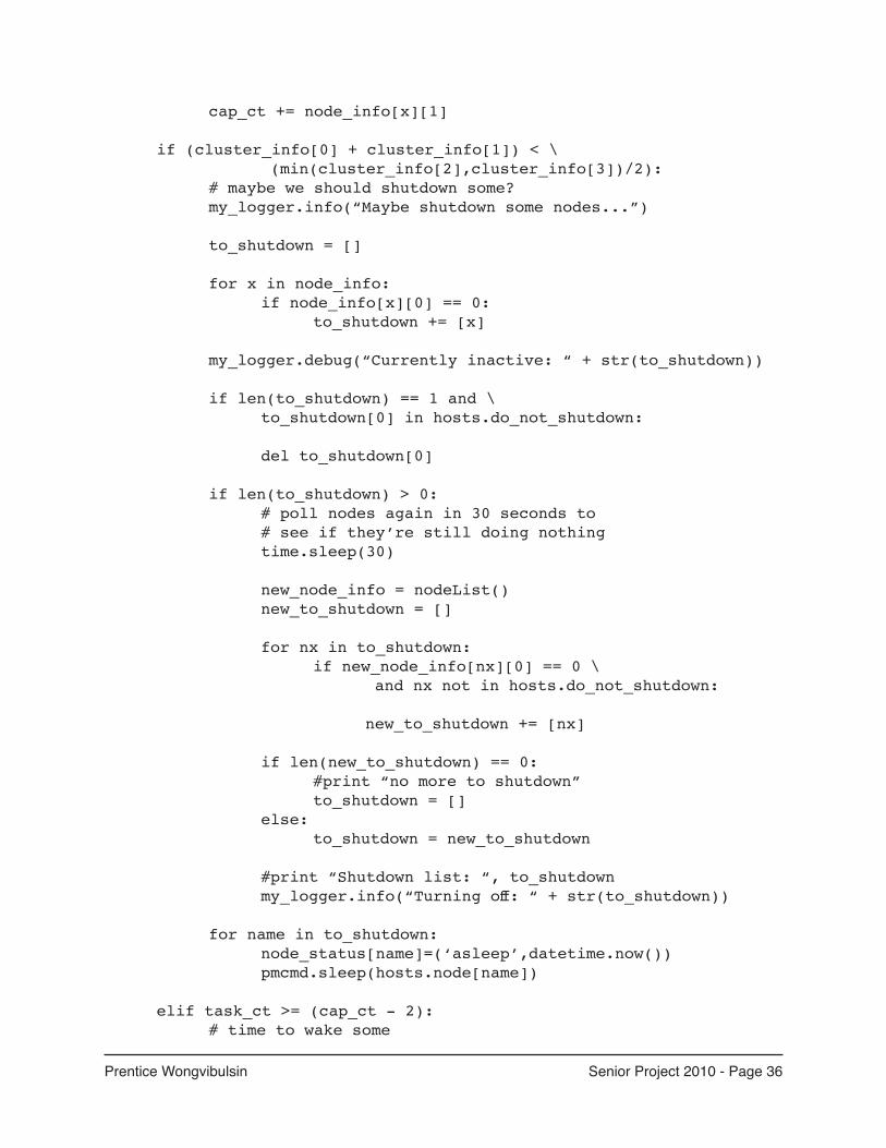
cap_ct += node_info[x][1] if (cluster_info[0] + cluster_info[1]) < \ (min(cluster_info[2],cluster_info[3])/2): # maybe we should shutdown some? my_logger.info(“Maybe shutdown some nodes...”)
to_shutdown = [] for x in node_info: if node_info[x][0] == 0: to_shutdown += [x]
my_logger.debug(“Currently inactive: “ + str(to_shutdown))
if len(to_shutdown) == 1 and \ to_shutdown[0] in hosts.do_not_shutdown:
del to_shutdown[0]
if len(to_shutdown) > 0: # poll nodes again in 30 seconds to # see if they’re still doing nothing time.sleep(30)
new_node_info = nodeList() new_to_shutdown = [] for nx in to_shutdown: if new_node_info[nx][0] == 0 \ and nx not in hosts.do_not_shutdown:
new_to_shutdown += [nx]
if len(new_to_shutdown) == 0: #print “no more to shutdown” to_shutdown = [] else: to_shutdown = new_to_shutdown
#print “Shutdown list: “, to_shutdown my_logger.info(“Turning off: “ + str(to_shutdown)) for name in to_shutdown: node_status[name]=(‘asleep’,datetime.now()) pmcmd.sleep(hosts.node[name])
elif task_ct >= (cap_ct - 2): # time to wake some

Prentice Wongvibulsin Senior Project 2010 - Page 37
my_logger.info(“We should wake some up...”) wake_list = []
for n in hosts.node: if n not in node_info: wake_list += [n]
random.shuffle(wake_list)
swake_list = []
for to_wake in wake_list: if (to_wake in node_status and \ node_status[to_wake] == ‘asleep’):
swake_list = [to_wake] + swake_list else: swake_list = swake_list + [to_wake]
my_logger.debug(“Offline hosts: “ + str(wake_list))
wake_list = swake_list
my_logger.debug(“Wake List: “ + str(wake_list))
if len(wake_list) >= 1: node_status[wake_list[0]] = (‘waking’, datetime.now()) pmcmd.wake(hosts.node[wake_list[0]]) if len(wake_list) >= 2: node_status[wake_list[1]] = (‘waking’, datetime.now()) pmcmd.wake(hosts.node[wake_list[1]])
handle = open(STATUS_FILENAME, ‘wb’) pickle.dump(node_status, handle) handle.close() my_logger.info(“goodbye.”)
if __name__ == “__main__”: main()
Prentice Wongvibulsin Senior Project 2010 - Page 38
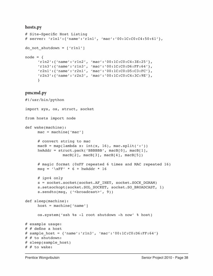
hosts.py# Site-Specific Host Listing# server: ‘r1n1’:{‘name’:’r1n1’, ‘mac’:’00:1C:C0:C4:50:61’},
do_not_shutdown = [‘r1n1’]
node = { ‘r1n2’:{‘name’:’r1n2’, ‘mac’:’00:1C:C0:C4:3E:25’}, ‘r1n3’:{‘name’:’r1n3’, ‘mac’:’00:1C:C0:D6:FF:64’}, ‘r2n1’:{‘name’:’r2n1’, ‘mac’:’00:1C:C0:D5:C3:FC’}, ‘r2n3’:{‘name’:’r2n3’, ‘mac’:’00:1C:C0:C4:3C:9E’}, }
pmcmd.py#!/usr/bin/python
import sys, os, struct, socket
from hosts import node
def wake(machine): mac = machine[‘mac’]
# convert string to mac macB = map(lambda x: int(x, 16), mac.split(‘:’)) hwAddr = struct.pack(‘BBBBBB’, macB[0], macB[1], macB[2], macB[3], macB[4], macB[5]) # magic format (0xFF repeated 6 times and MAC repeated 16) msg = ‘\xFF’ * 6 + hwAddr * 16
# ipv4 only s = socket.socket(socket.AF_INET, socket.SOCK_DGRAM) s.setsockopt(socket.SOL_SOCKET, socket.SO_BROADCAST, 1) s.sendto(msg, (‘<broadcast>’, 9))
def sleep(machine): host = machine[‘name’] os.system(‘ssh %s -l root shutdown -h now’ % host)
# example usage:# # define a host# sample_host = {‘name’:’r1n3’, ‘mac’:’00:1C:C0:D6:FF:64’}# # to shutdown:# sleep(sample_host)# # to wake:

Prentice Wongvibulsin Senior Project 2010 - Page 39
# wake(sample_host)
def main(): func = {‘wake’:wake, ‘sleep’:sleep} if len(sys.argv) != 3: print “usage: ./pmcmd.py [cmd] [host]” elif sys.argv[2]==”all”: for n in node: func[sys.argv[1]](node[n]) else: func[sys.argv[1]](node[sys.argv[2]])
if __name__ == “__main__”: main()
Prentice Wongvibulsin Senior Project 2010 - Page 40
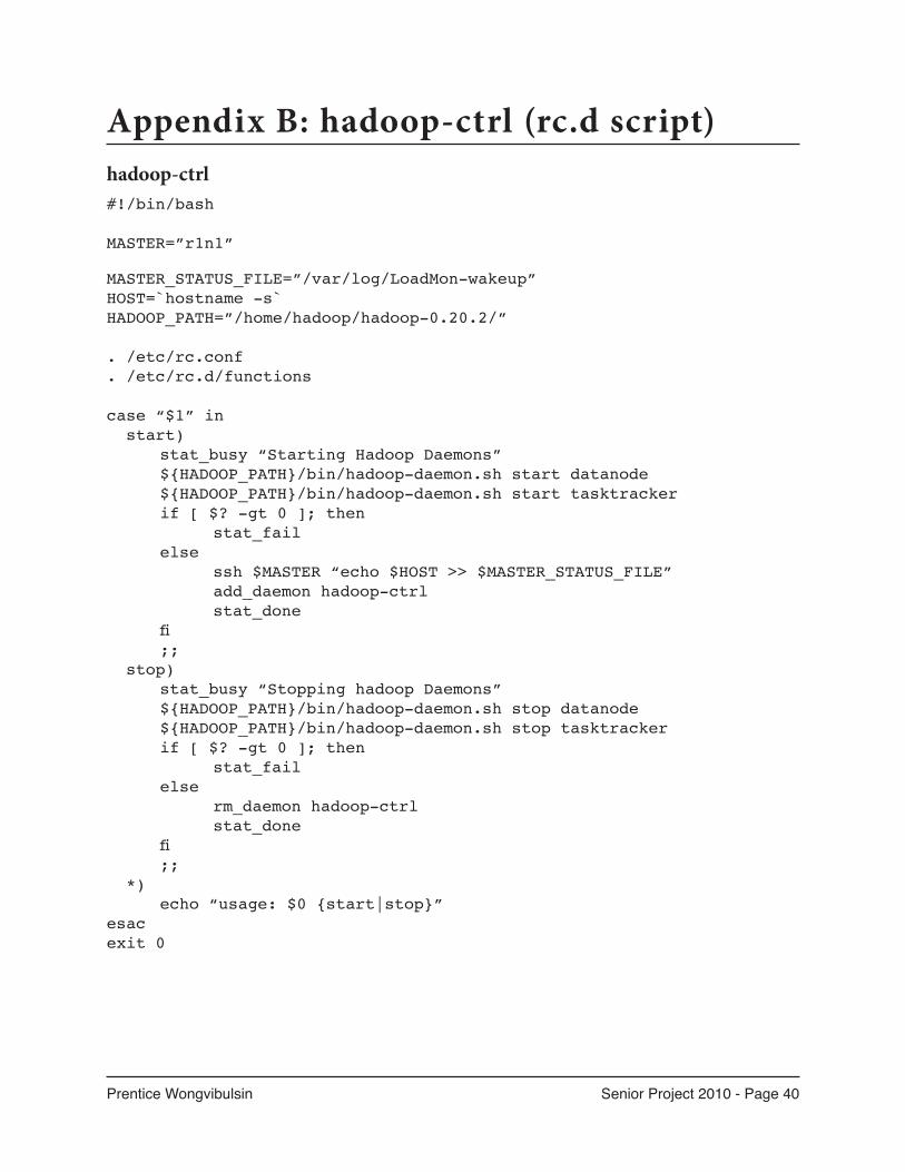
Appendix B: hadoop-ctrl (rc.d script)hadoop-ctrl#!/bin/bash
MASTER=”r1n1”
MASTER_STATUS_FILE=”/var/log/LoadMon-wakeup”HOST=`hostname -s`HADOOP_PATH=”/home/hadoop/hadoop-0.20.2/”
. /etc/rc.conf
. /etc/rc.d/functions
case “$1” in start) stat_busy “Starting Hadoop Daemons” ${HADOOP_PATH}/bin/hadoop-daemon.sh start datanode ${HADOOP_PATH}/bin/hadoop-daemon.sh start tasktracker if [ $? -gt 0 ]; then stat_fail else ssh $MASTER “echo $HOST >> $MASTER_STATUS_FILE” add_daemon hadoop-ctrl stat_done fi ;; stop) stat_busy “Stopping hadoop Daemons” ${HADOOP_PATH}/bin/hadoop-daemon.sh stop datanode ${HADOOP_PATH}/bin/hadoop-daemon.sh stop tasktracker if [ $? -gt 0 ]; then stat_fail else rm_daemon hadoop-ctrl stat_done fi ;; *) echo “usage: $0 {start|stop}”esacexit 0
Prentice Wongvibulsin Senior Project 2010 - Page 41
Appendix C: Sparse Load Job Runnerrunner.py#!/usr/bin/pyhton
import osimport time
from datetime import datetimefrom datetime import timedelta
HADOOP_PATH=”/home/hadoop/hadoop-0.20.2/”
njobs = 0start = datetime.now()end = start + timedelta(minutes=55)
last_job = datetime.now() - timedelta(1)
while datetime.now() < end: if last_job < datetime.now() - timedelta(minutes=5): print “Starting job...” print “Approx end time “, end last_job = datetime.now() njobs+=1 os.system(HADOOP_PATH + “bin/hadoop jar “ + HADOOP_PATH \ + “hadoop-0.20.2-examples.jar pi 100 500”) time.sleep(30)
print “Done! “, njobs, “ completed in “, datetime.now() - start
Prentice Wongvibulsin Senior Project 2010 - Page 42
Appendix D: Add new node scriptaddMe.sh# ./addMe [hostname] [ip] [server]
echo “Don’t forget to set hostname in /etc/rc.conf and /etc/hosts.”
#generate new keyssh-keygen -t dsa -P ‘’ -f ~/.ssh/id_dsa
#copy public key to serverscp ~/.ssh/id_dsa.pub root@$3:~/$1.key
#add me to authorized keys on this host and servercat ~/.ssh/id_dsa.pub >> ~/.ssh/authorized_keysssh $3 -l root “cat ~/$1.key >> ~/.ssh/authorized_keys”
#add me to slaves filessh $3 -l root “echo $1 >> hadoop-0.20.2/conf/slaves”
#add me to hosts filessh $3 -l root “echo $2 $1 >> /etc/hosts”


![Cluster Computing Architecture Intel Labs - 01.org · Cluster Computing Architecture 10 *[Neo4j] ... GraphBuilder makes it easy. ... Our Wikipedia Graphs 38 Cluster Computing Architecture](https://img.pdfslide.net/doc/110x75/5b552dd37f8b9a0d398dead8/cluster-computing-architecture-intel-labs-01org-cluster-computing-architecture.jpg)