Embed Size (px)
Citation preview

This article was downloaded by: [Stanford University Libraries]On: 04 October 2012, At: 13:44Publisher: Taylor & FrancisInforma Ltd Registered in England and Wales Registered Number: 1072954 Registered office: Mortimer House,37-41 Mortimer Street, London W1T 3JH, UK
Numerical Heat TransferPublication details, including instructions for authors and subscription information:http://www.tandfonline.com/loi/unht19
EFFICIENT SEMI-IMPLICIT SOLVING ALGORITHM FORNINE-DIAGONAL COEFFICIENT MATRIXMilovan Peric aa Lehrstuhl für Strömungsmechanik, Universität Erlangen-Nürnberg, Egerlandstrasse 13,Erlangen, F.R., 8520, Germany
Version of record first published: 05 Apr 2007.
To cite this article: Milovan Peric (1987): EFFICIENT SEMI-IMPLICIT SOLVING ALGORITHM FOR NINE-DIAGONAL COEFFICIENTMATRIX, Numerical Heat Transfer, 11:3, 251-279
To link to this article: http://dx.doi.org/10.1080/10407788708913554
PLEASE SCROLL DOWN FOR ARTICLE
Full terms and conditions of use: http://www.tandfonline.com/page/terms-and-conditions
This article may be used for research, teaching, and private study purposes. Any substantial or systematicreproduction, redistribution, reselling, loan, sub-licensing, systematic supply, or distribution in any form toanyone is expressly forbidden.
The publisher does not give any warranty express or implied or make any representation that the contentswill be complete or accurate or up to date. The accuracy of any instructions, formulae, and drug doses shouldbe independently verified with primary sources. The publisher shall not be liable for any loss, actions, claims,proceedings, demand, or costs or damages whatsoever or howsoever caused arising directly or indirectly inconnection with or arising out of the use of this material.
Numerical Heat Transfer, vol. 11, pp. 251-279, 1987
EFFICIENT SEMI-IMPLICIT SOLVING ALGORITHM FOR NINE-DIAGONAL COEFFICIENT MATRIX
Milovan Peric Lehrstuhl fur Stromungsmechanik. Universitut Erlangen-Niirnberg, Egerlandstrasse 13. 8520 Erlangen. F.R. Germany
In numerical calculations of fluid flows and heat transfer it is often necessary to solve a system of algebraic equations with a nine-diagonal coefficient matrix. Two examples are the diffusion and pressure-correction equations when discretized on nonorthogonal grids. A method of solving such systems of equations, based on the strongly implicit procedure of Stone [I] for five-diagonal mohifes, is presented. It operates on the upper and lower triangular matrices with only seven nonzero diag- onals, thus requiring less storage and computing time per iferalion than the alter- native extensions of the strongb implicit procedure to nine-diagonal coefficient ma- bices. It $ aLFo more eflicient than the ollernaIive methoak-for the kind of equations studied-when the missing diagonals in the upper and lower triangular matrices correspond to points lying in "sharp" corners of a compularional molecule. Results of various test calcuhfions and comparisons of performance with alternative solvers are presented to support this view. The proposed solver can also be applied to five- diagonal matrix problems, in which case it reduces to the strongly implicit procedure of Stone [I].
INTRODUCTION
In recent years much effort has been devoted to developing procedures for the numerical prediction of fluid flow and heat transfer in complex geometries [2-71. For many practical problems the use of orthogonal body-fitted coordinates leads to an unfavorable distribution of grid lines in the numerical grid. The alternative is to use general nonorthogonal coordinates, which offer far greater control over the dis- tribution of grid lines, as discussed, e.g., in [4]. In this case the differential equations become significantly more complex than their Cartesian counterparts. This will be demonstrated on the heat conduction equation:
div(r, grad 4) + s+ = 0 (1)
In the Cartesian coordinate system (y',y2) this equation reads
The first version of this paper was written during the author's employment at the Institute of Process. Power and Environmental Engineering, University of Sarajevo, Yugoslavia.
The author thanks Dr. A. D. Gosman of Imperial College, London, and Dr. I . Demirdzic of the Faculty of Mechanical Engineering. University of Sarajevo, for providing computer code for fluid flow prediction on nonorthogonal grids.
Copyright O 1987 by Hemisphere Publishing Corporation 25 1
Dow
nloa
ded
by [
Stan
ford
Uni
vers
ity L
ibra
ries
] at
13:
44 0
4 O
ctob
er 2
012
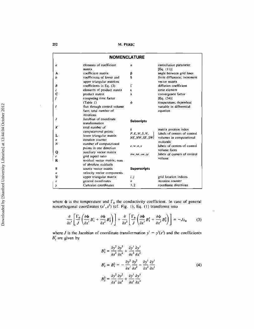
252 M. PERIC
NOMENCLATURE
elements o f coefficient matrix coefficient matrix coefficients o f lower and upper triangular matrices coefficients in Eq. (3) elements of product matrix product matrix computing time factor (Table I ) flux through control volume face; total number o f iterations Jacobian o f coordinate transformation total number o f computational points lower triangular matrix iteration counter number o f computational points in one direction auxiliary vector matrix grid aspcct ratio residual vector matrix; sum o f absolute residuals source vector matrix velocity vector components upper triangular matrix general coordinates Cartesian coordinates
Subscripts
k P.E,W,S,N, NE,NW,SE,SW 1 e , w . n . s
nw.ne.sw.se
Superscripts
cancellation parameter
IEq. (1 1)1 angle between grid lines finite difference; increment vector matrix diffusion coefficient error element convergence factor
[Eq. MI temperature; dependent variable in differential equation
matrix position index labels o f centers o f control volumes in computational molecule labels o f centers o f control volume faces labels of corners o f control volume
grid location indices iteration counter coordinate directions
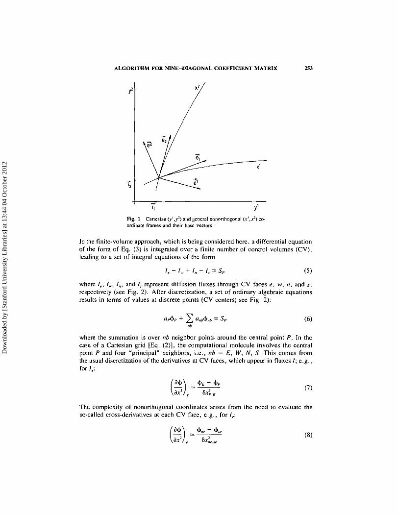
where I+ is the temperature and r+ the conductivity coefficient. In case of general nononhogonal coordinates (x ' ,x2) (cf. Fig. I ) , Eq. ( I ) transforms into
where J is the Jacobian of coordinate transformation y' = y i ( k ) and the coefficients B: are given by
ay2 ay2 aYL ayl B ~ = B : = a.2 axZ ax2 ax'
ay2 ay2 ay' ayl @ = - - +-- ax' ax' ax' ax'
Dow
nloa
ded
by [
Stan
ford
Uni
vers
ity L
ibra
ries
] at
13:
44 0
4 O
ctob
er 2
012
ALGORITHM FOR NINE-DIAGONAL COEFFICIENT MATRIX
Fig. 1 Cartesian ( y ' , y2 ) and general nonorthogonal (x',x2) co- ordinate frames and their base vectors.
In the finite-volume approach, which is being considered here, a differential equation of the form of Eq. (3) is integrated over a finite number of control volumes (CV), leading to a set of integral equations of the form
where I , , I,., I, , and I, represent diffusion fluxes through CV faces e, w , n , and s , respectively (see Fig. 2 ) . After discretization, a set of ordinary algebraic equations results in terms of values at discrete points (CV centers; see Fig. 2) :
where the summation is over nb neighbor points around the central point P. In the case of a Cartesian grid [Eq. (Z)], the computational molecule involves the central point P and four "principal" neighbors, i.e., nb = E, W , N, S. This comes from the usual discretization of the derivatives at CV faces, which appear in fluxes I ; e.g., for I,:
The complexity of nonorthogonal coordinates arises from the need to evaluate the so-called cross-derivatives at each CV face, e.g., for I,:
Dow
nloa
ded
by [
Stan
ford
Uni
vers
ity L
ibra
ries
] at
13:
44 0
4 O
ctob
er 2
012

Fig. 2 Typical computational molecule and grid labeling scheme
Values such as I$, are usually obtained by linear interpolation among the four sur- rounding points, in this case N, P, NE, and E. Thus the computational molecule extends to include the "comer" points NE, NW, SE, and SW (Fig. 2). The magnitude of coefficients for the comer points increases as the angle of grid line inclination P departs from orthogonality; it is also influenced by the grid aspect ratio 131.
The set of Eq. (6) can be written in matrix form as
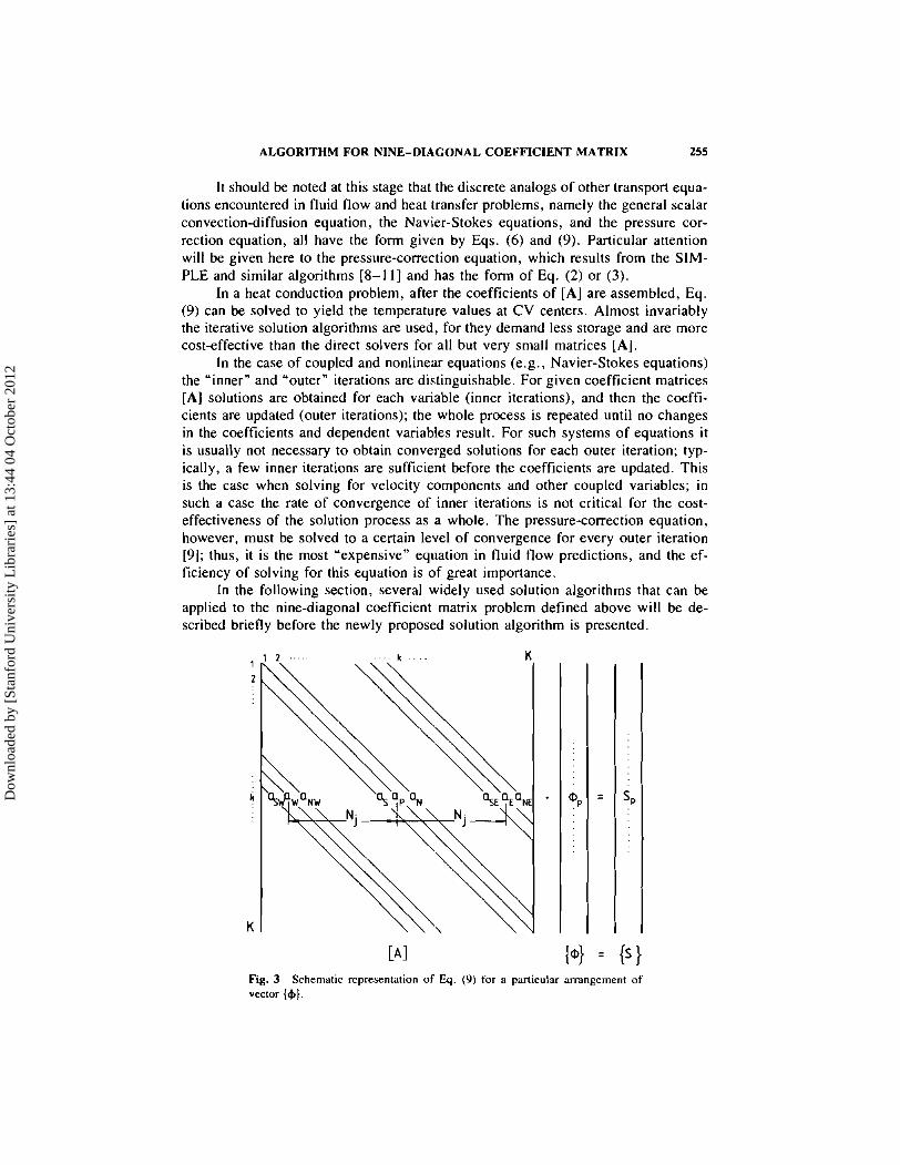
Here {+} represents the temperature field at discrete locations in the domain, ar- ranged in vector form, {S} is a similar vector containing source terms, and [A] is the coefficient matrix. The latter is a square matrix with dimensions K X K, where K is the total number of computational points. However, in every row there are only five (for orthogonal grids) or nine (for nonorthogonal grids) nonzero coefficients [Eq. (6)]. The arrangement of nonzero coefficients in [A] depends on the way in which the vector {+} is formed. The numerical grid is typically indexed as shown in Fig. 2, with index i in the direction of the x' coordinate ranging from 1 to Ni*; similarly, in the .I? direction the index j ranges from I to N,, and the central point P then has grid coordinates (i, j ) .
I f the vector {+} is arranged so that the points follow each other along one line, line after line in given order (e.g., from j = I to N, for i = 1 and in the same way for lines i = 2 to N,), the matrix [A] will then have nonzero coefficients along five or nine diagonals, as shown for the above example in Fig. 3.
*Note that indices 1 and N; denote the boundary points and 2 to N,-I centers of control volumes bcrwcen thc two boundaries; equations of the form (6) exist for these "interior" points only.
Dow
nloa
ded
by [
Stan
ford
Uni
vers
ity L
ibra
ries
] at
13:
44 0
4 O
ctob
er 2
012
ALGORITHM FOR NINE-DIAGONAL COEFFICIENT MATRIX 255
I t should be noted at this stage that the discrete analogs of other transport equa- tions encountered in fluid flow and heat transfer problems, namely the general scalar convection-diffusion equation, the Navier-Stokes equations, and the pressure cor- rection equation, all have the form given by Eqs. (6) and (9). Particular attention will be given here to the pressure-correction equation, which results from the SIM- PLE and similar algorithms 18-1 I ] and has the form of Eq. (2) or (3).
In a heat conduction problem, after the coefficients of [A] are assembled, Eq. (9) can be solved to yield the temperature values at CV centers. Almost invariably the iterative solution algorithms are used, for they demand less storage and are more cost-effective than the direct solvers for all but very small matrices [A].
In the case of coupled and nonlinear equations (e.g., Navier-Stokes equations) the "inner" and "outern iterations are distinguishable. For given coefficient matrices [A] solutions are obtained for each variable (inner iterations), and then the coeffi- cients are updated (outer iterations); the whole process is repeated until no changes in the coefficients and dependent variables result. For such systems of equations it is usually not necessary to obtain converged solutions for each outer iteration; typ- ically, a few inner iterations are sufficient before the coefficients are updated. This is the case when solving for velocity components and other coupled variables; in such a case the rate of convergence of inner iterations is not critical for the cost- effectiveness of the solution process as a whole. The pressure-correction equation, however, must be solved to a certain level of convergence for every outer iteration [9]; thus, it is the most "expensive" equation in fluid flow predictions, and the ef- ficiency of solving for this equation is of great importance.
In the following section, several widely used solution algorithms that can be applied to the nine-diagonal coefficient matrix problem defined above will be de- scribed briefly before the newly proposed solution algorithm is presented.
Fig. 3 Schematic representation of Eq. (9) for a particular arrangement of vector {$}.
Dow
nloa
ded
by [
Stan
ford
Uni
vers
ity L
ibra
ries
] at
13:
44 0
4 O
ctob
er 2
012

REVIEW OF SOME EXISTING SOLUTION ALGORITHMS
One of the most widely used iterative solution algorithms is the so-called line- by-line (LBL) algorithm, which employs the tridiagonal matrix algorithm (TDMA) (e.g., see 1101). The TDMA gives the exact solution for a three-diagonal coefficient matrix, which would result in a one-dimensional heat conduction problem. When treating two-dimensional problems by the LBL approach, the TDMA operates with coefficients corresponding to points along a particular line, while the contribution from coefficients of points on neighbor lines is calculated as a known quantity from 4 values obtained in a previous iteration and added to the source term. The grid is typically scanned line by line, first in one direction (e.g., along lines of constant grid index i) and then in the other direction. This solver does not demand much extra storage (two one-dimensional arrays) and is efficient for small matrices. How- ever, as will be demonstrated later, the rate of convergence for nine-diagonal coef- ficient matrices is rather low.
A more efficient solver for two-dimensional problems has been proposed by Stone 11 1 . His strongly implicit procedure (SIP) is designed for five-diagonal ma- trices, which would result, e.g., from the discretization procedure described in the Introduction on orthogonal grids. Two triangular matrices, [L] for lower and [U] for upper, are defined so that they have nonzero coefficients on the same diagonals as the matrix [A]. Instead of Eq. (9), the following equation is then solved:
The product matrix [L] .'[u] has two extra diagonals, corresponding to points NW, SE or NE, SW, depending on the arrangement of the vector {+}. The coefficients of the matrices [L] and [U] are chosen so that the product matrix is a good approxi- mation of the matrix [A], and through a suitable iteration procedure (described later) the solution of Eq. (9) can be obtained. The "good approximationn is achieved by partially canceling the influence of the two extra diagonals in the product matrix through approximations of the following form:
where a is a parameter in the range 0-1. The SIP solver requires storage of five coefficients of matrices [L] and [U] per
computational point. Although strictly speaking it IS designed for five-diagonal ma- trices, it can be applied to nine-diagonal ones as well; however, as will be shown later, the rate of convergence deteriorates rapidly as the magnitude of the comer coefficients increases.
The SIP algorithm can be directly extended to nine-diagonal matrices, as done by Jacobs [I21 and Schneider and Zedan [13], among others. When the two trian- gular matrices are chosen such that they have nonzero coefficients on the same di- agonals as matrix [A], the product matrix has nonzero coefficients on four extra diagonals, e.g., corresponding to points marked by open circles in Fig. 2 for the
Dow
nloa
ded
by [
Stan
ford
Uni
vers
ity L
ibra
ries
] at
13:
44 0
4 O
ctob
er 2
012

ALGORITHM FOR NINE-DIAGONAL COEFFICIENT MATRIX 257
arrangement of vector {+} mentioned above (cf. Fig. 3). The influence of these extra coefficients is partially canceled by expressing the 4 values that they multiply through values at neighbor points included in the computational molecule. Jacobs 1121 and Schneider and Zedan [I31 use the following approximation formulas for $,, and 4, (cf. Fig. 2):
For the remaining two points Jacobs [I21 chose expressions of the same form, which he found to be the best of several alternatives he tried: thus:
Schneider and Zedan [13], on the other hand, chose the following expressions for these two points:
Both methods require storage of nine coefficients of [L] and [U] per computational point and are-like the SIP-more or less sensitive to the choice of the parameter a. Jacobs 1121 tried various approximation formulas similar to Eqs. (13) and (14) and found that they significantly affect the convergence property of the resulting solution algorithm. Schneider and Zedan [I31 claim to have found a better choice in Eq. (14), resulting in reduction of sensitivity to the value of a. If applied to a five-diagonal coefficient matrix [A], their method-which they called modified strongly implicit (MS1)-uses seven nonzero coefficients in triangular matrices and hence does not reduce to the SIP.
In the next section a newly developed solution method for nine-diagonal ma- trices, which also stems from the SIP, will be presented. It is designed to provide fast convergence when solving differential equations of the form of Eq. (1) discre- tized on nonorthogonal grids, where the comer coefficients result from the discre- tization of cross-derivatives as in Eq. (8).
A NEW SOLUTION METHODOLOGY
In the early stage of this study the extension of the SIP methodology to nine- diagonal matrices was pursued by the same path used by Jacobs [I 21 and Schneider and Zedan 1131. It was noted, however. that there are two triangular matrices [L] and [U] whose product gives a nine-diagonal matrix of exactly the same form as the coefficient matrix [A] of Eq. (9). These two triangular matrices have nonzero coef- ficients on seven diagonals only, which coincide with the corresponding nonzero diagonals in [A]. The two diagonals left out are those corresponding to the two
Dow
nloa
ded
by [
Stan
ford
Uni
vers
ity L
ibra
ries
] at
13:
44 0
4 O
ctob
er 2
012
opposite corner points, NW-SE or NE-SW, depending on the arrangement of points in the vector {$}. The analysis that follows refers to the arrangement shown sche- matically in Fig. 3; i.e. the matrix position index k , which corresponds to grid lo- cation (i,j), is calculated as k = (i - 1)N, + j , where j changes from 1 to N, and i from I to N;. This arrangement will be denoted as a left-to-right (LR) sweep; for thc alternative arrangement, in which k = (N, - i)N, + j , with j changing as before but i changing backward from Nj to I [denoted here as a right-to-left (RL) sweep] the essential steps will be outlined in the Appendix.
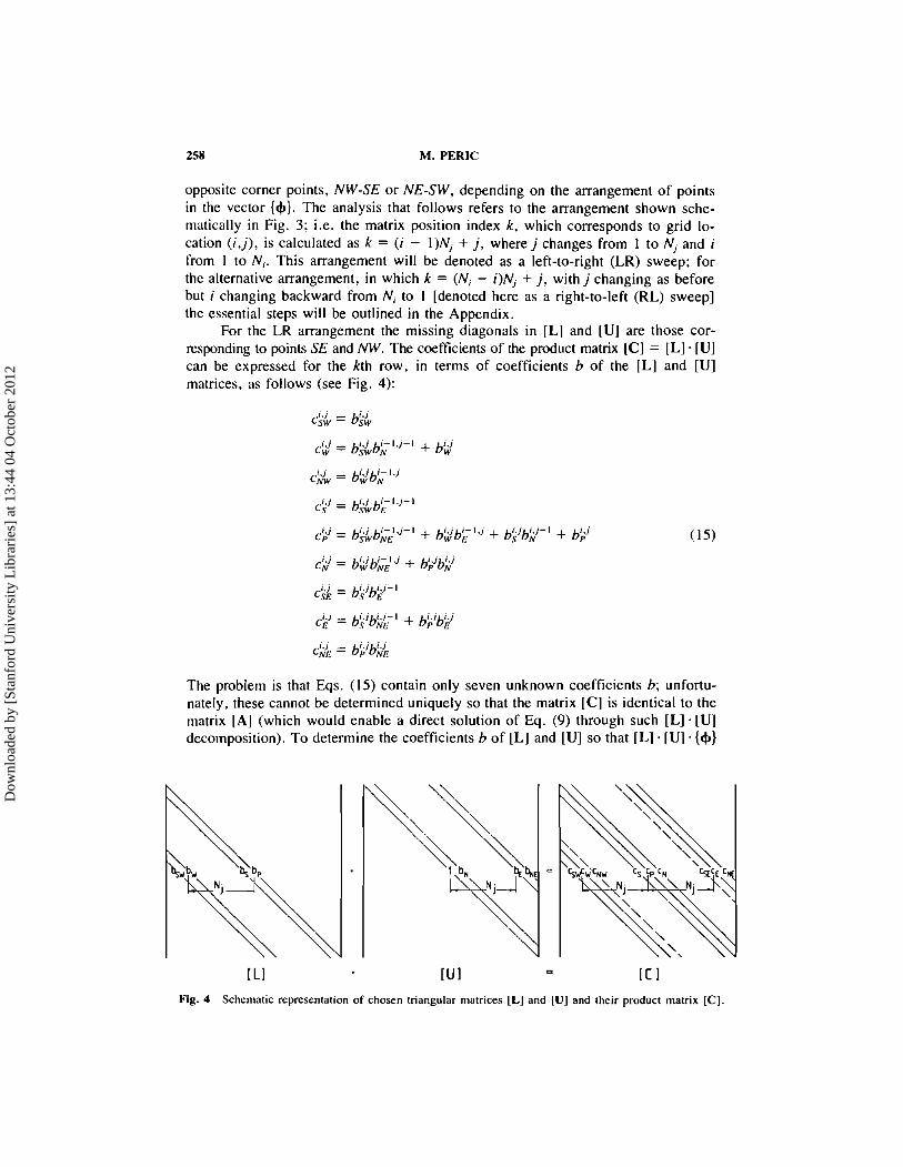
For the LR arrangement the missing diagonals in [L] and [U] are those cor- responding to points SE and NW. The coefficients of the product matrix [C] = [L] . [U] can be expressed for the kth row, in terms of coefficients b of the IL1 and [U] matrices, as follows (see Fig. 4):
The problem is that Eqs. (15) contain only seven unknown coefficients b; unfortu- nately, these cannot be determined uniquely so that the matrix [C] is identical to the matrix [A] (which would enable a direct solution of Eq. (9) through such [L]. [U] decomposition). To determine the coefficients b of [L] and IU] so that [L] . [U] . {&)
Fig. 4 Schematic representation of chosen triangular matrices [L] and [Ul and their product mavix [C]
Dow
nloa
ded
by [
Stan
ford
Uni
vers
ity L
ibra
ries
] at
13:
44 0
4 O
ctob
er 2
012

ALGORITHM FOR NINE-DIAGONAL COEFFICIENT MATRIX 259
is a reasonable approximation to [A] . ($1, the following two-step procedure may be adopted.
Step 1
If the values of the dependent variable + at points NW and SE-for which there are no coefficients b-are assumed to satisfy the following relations:*
then Eq. (6) for location (i,j') can be rewritten as follows:'
This can be seen as an approximation to Eq. (6 ) , which can be written in matrix form as
Matrix [A'], which represents an approximation to matrix [A] of Eq. (9), now has nonzero coefficients on seven diagonals, which correspond to those of the [L] and [U] matrices:
a; = a, -t aa,
ak = a, t aaNw
a; = a, + aa,,
a; = a, + aa,,
OLE = ONE
aiw = asw
Step 2
The product matrix [C] = [L] . [U] has nonzero coefficients on nine diagonals, including those corresponding to points NW and SE. To calculate the coefficients b
*This is one of the many possible ways to approximate the + values at points NW and SE through the values at neighbor points. Equations (16) are identical to those used by Stone [ I ] [cf. Eq. ( I I )) , which Jacobs [I21 also found to be of the most general validity.
'The superscript indices for coefficients are omitted for clarity; wherever not included. index i , j is assumed.
Dow
nloa
ded
by [
Stan
ford
Uni
vers
ity L
ibra
ries
] at
13:
44 0
4 O
ctob
er 2
012
260 M. PERIC
so that [C] . ($1 represents a reasonable approximation to [A'] . {$}, the influence of the two additional coefficients may be partially cancelled by again using Eqs. (16), as outlined below.
Equation (17) can be approximated by
The last two terms on the left side of Eq. (20) are small compared to the other terms if the approximations of Eqs. (16) are valid. Equation (20) thus represents an ap- proximation to Eq. (17), which is an approximation to Eq. (6) arrived at by using the same substitution formulas (16). When this equation is rearranged and the coef- ficients of corresponding +'s are set equal to the corresponding coefficients c of Eq. (IS), there results the following set of equations from which the coefficients b can be calculated uniquely for each point:
Thus the coefficients of matrices [L] and [U] have been determined, and the equation
can now be solved by a rather simple inversion of triangular matrices. However, Eq. (22) is not exactly the same as Eq. (9), whose solution is being sought; therefore, an iterative procedure must be devised that,will lead to the solution satisfying Eq. (9). A method suggested by Stone [I] can be applied here, too.
First, Eq. (9) can be rewritten as
Dow
nloa
ded
by [
Stan
ford
Uni
vers
ity L
ibra
ries
] at
13:
44 0
4 O
ctob
er 2
012

ALGORITHM FOR NINE-DIAGONAL COEFFICIENT MATRIX 261
If n is an iteration counter, the iterative procedure can be arranged as follows:
By introducing two new vector matrices, namely the increment vector 16) and the residual vector {R},
and
we obtain the following equation:
[L] . [U] .{6") = {R")
Multiplying Eq. (27) by [L]-' gives
where
{a") = [L] - ' . {Rn) (29)
Furthermore, an expression is obtained for the increment vector {S}:
The elements of vector matrices {Q} and {S} are easily obtained from Eqs. (29) and (30) by forward and backward substitution:
Finally, Eq. (25) can be used to update the 4 field from {+"I to {+"+'}. The process is repeated-by starting from a guessed field {+'}-until a prescribed convergence criterion is satisfied. In this study the criterion defined below was used.
If R, is the sum of absolute values of all elements of residual vector {R") after the nth iteration,
Dow
nloa
ded
by [
Stan
ford
Uni
vers
ity L
ibra
ries
] at
13:
44 0
4 O
ctob
er 2
012
then the iteration process is terminated when the following criterion is satisfied:
Here A is a prescribed small number whose order of magnitude determines the ac- curacy of the solution. The rate of convergence depends on several factors, which will be discussed in the next section.
CONVERGENCE RATE ANALYSIS
The solution algorithm presented in the previous section reduces to that of Stone I I I when the corner coefficients are zero, i.e., when the coefficient matrix is five- diagonal (step I becomes redundant in that case). For the kinds of equation and discretization procedure considered here, this happens when the numerical grid be- comes orthogonal. The rate of convergence is then influenced primarily by the choice of parameter a, i.e., the validity of replacement formulas* (16). Other factors are the grid aspect ratio r,, defined as
where 6x' and 6x2 are the grid spacings in the direction of coordinates x ' and 2, respectively, and the actual problem under consideration. More details of the per- formance of the SIP solver for five-diagonal matrices can be found elsewhere [ I , 131; this will also be addressed in the next section, when the results of test calcu- lations are presented.
Attention will be turned here to the case of nine-diagonal coefficient matrices ., resulting from the discretization of the diffusion operator on nonorthogonal grids, as indicated in the Introduction. It will be shown that for such matrices the DroDosed . . method converges especially fast when the vector {+) is arranged so that approxi- mations of the form of Eq. (16) are applied to points that lie in "sharp" comers of the computational molecule (see Fig. 2).
First, comparing Eq. (17) of step 1 with Eq. (6) indicates that they differ by the term
where 6 4 , and 6 4 , are the differences between the left and right sides of Eq. (16), and their magnitude depends solely on the value of a.
*When a = 0 the coefficients of matrices [A] and [C] corresponding to the nonzero diagonals in metrices IL] and [U] are set equal, and the extra two coefficients in [C] are accepted as they come out. with no compensation for their influence.
Dow
nloa
ded
by [
Stan
ford
Uni
vers
ity L
ibra
ries
] at
13:
44 0
4 O
ctob
er 2
012
ALGORITHM FOR NINE-DIAGONAL COEFFICIENT MATRIX 263
Second, comparing Eq. (20) of step 2 with Eq. (17) of step 1 indicates that they differ by the term
Thus, the difference between Eq. (20), which is actually being solved, and Eq. (6) , whose solution is being sought, appears to be
The quantity E determines the "error" introduced by the approximations in steps I and 2. The magnitude of this error, according to Eq. (38), depends on the magnitude of the 641"s and the difference between the coefficients of matrices [A] and [C] that multiply them. The former, as already noted, depends on the choice of a ; the latter depends on the magnitude and sign of the corresponding coefficients a and c , which further depend on the arrangement of points in vector {I$}. This second influence can be exploited to advantage, as will now be explained.
The magnitude of the comer coefficients aw, a,,, a,,, as,, as noted in the Introduction, depends on the angle P between grid lines and the cell aspect ratio r,. Their sign, however, depends on the angle P only and is positive if the point lies in a sharp comer of the computational molecule (Fig. 2) and negative otherwise (the coefficients of principal neighbors E , W, N , and S are-except in cases of extreme nonorthogonality or aspect ratio-always negative; e.g., see 131). The coefficients b of matrices [L] and [U] typically bear the sign of and are similar in magnitude to the corresponding coefficients a. Since the coefficients cNw and csE are made of prod- ucts of the bw, bN and b,, b,, respectively [Eq. (15)], it appears that their sign is normally positive, irrespective of the angle P. Thus, depending on the sign of a,, and a,,, the magnitude of the terms in parentheses in Eq. (38) is equal to either the sum or the difference of their individual magnitudes:
Therefore, the total error E of Eq. (38)-for a given value of a-is much smaller if points NW and SE lie in sharp comers of the computational molecule (P > 90"; see Fig. 2), since then the errors introduced through the approximations of steps I and 2 tend to partially cancel. The same is true for the RL arrangement of vector {I$} when p < 90°, since then the approximations mentioned above are applied to points NE and SW.
The analysis above suggests that convergence should be much faster for the appropriate arrangement of vector {+}: i.e., the RL for P < 90" and LR for P > 90". That this is indeed the case will be demonstrated in the next section, where the results of several test calculations are presented; the influence of a and the problem dependence are also highlighted.
Dow
nloa
ded
by [
Stan
ford
Uni
vers
ity L
ibra
ries
] at
13:
44 0
4 O
ctob
er 2
012

VALIDATION OF THE METHOD
In this section results of several test calculations will be presented. The aim of thcse calculations is to check the validity of the analysis presented in the preceding section and to compare the performance of the ~ r o ~ o s e d solver with that of similar existing solvers. Four different test cases were set up. Before the results are pre- sented, each of these cases will be described briefly.
Case I involves solution of the diffusion equation with no sources [Eq. (311 on a solution domain defined in Fig. 5. Four variants were studied; the height of a solution domain H was kept constant, H = 0.8 m, while the angle P and length L were varied as follows: for L = I m, P = 90°, 60°, and 45", and for L = 10 m, P = 45". The boundary conditions were a given temperature at two opposite (isother- mal) walls and zero normal gradient at the other two (adiabatic) walls, as indicated in Fig. 5. The diffusion coefficient r+ was set to I and kept constant over the solution domain. Uniform grids of 20 X 20 CV were used in all cases.
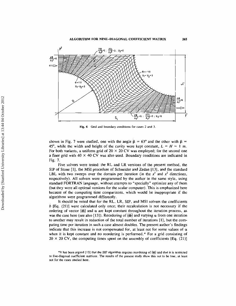
Case 2 also involves solution of the diffusion equation without sources, but in a more complex geometry, shown in ~ i g . 6. It represents a symmetry unit of a cross section of a staggered tube bank, with the global dimensions and a nonuniform 33 x 20 CV grid, shown in Fig. 6. The boundary conditions were isothermal tube walls (with different temperatures) and zero normal gradients across all symmetry bound- aries. The diffusion coefficient To was uniform over the domain.
Case 3 involves solution of the pressure-correction equation during flow cal- culations for the tube bank geometry shown in Fig. 6. For the velocity components, antisymmetric periodic conditions at inlet and outlet were assumed, while conditions at other boundaries were taken as indicated in Fig. 6. For the pressure-correction equation, a zero gradient condition was applied at all boundaries.
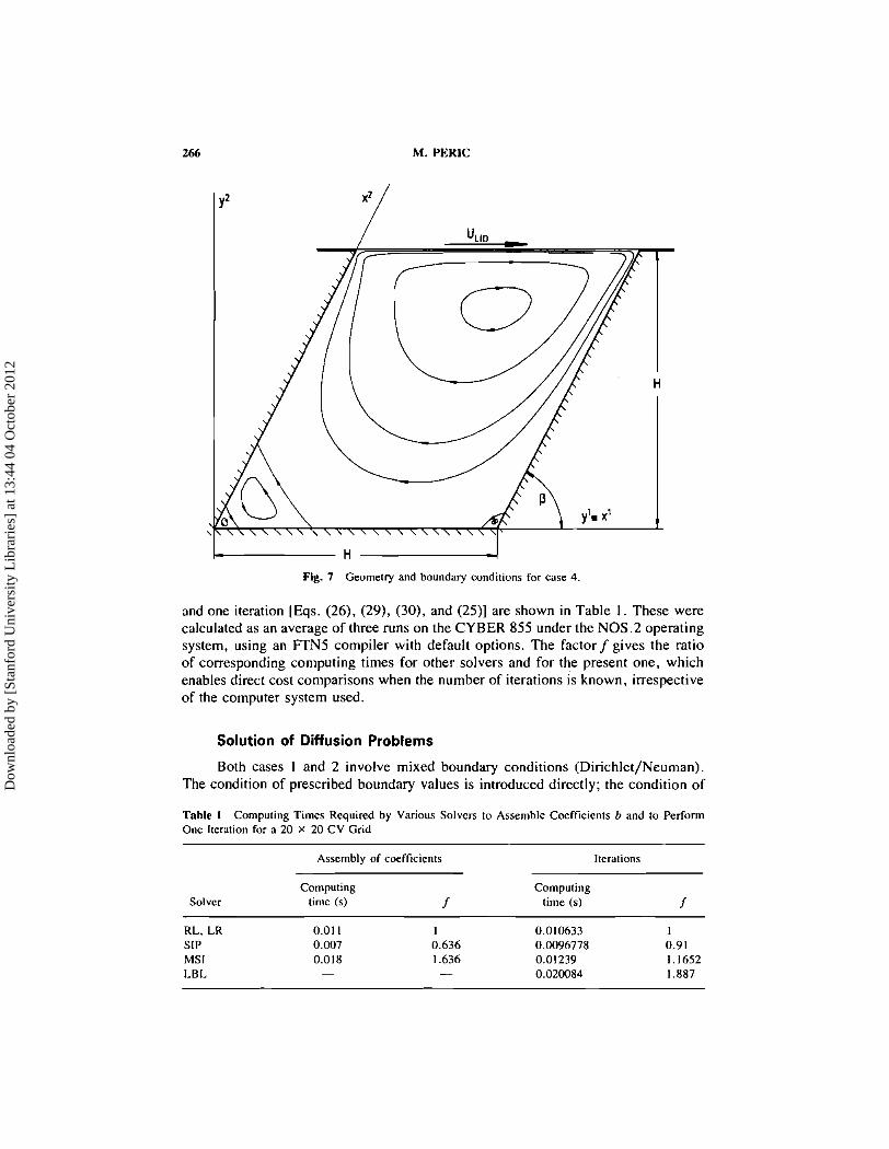
Finally, case 4 involves solution of the pressure-correction equation in calcu- lations of laminar lid-driven flow in cavities. Two variants of the basic geometry
Fig. 5 Geometry and boundary conditions for case I .
Dow
nloa
ded
by [
Stan
ford
Uni
vers
ity L
ibra
ries
] at
13:
44 0
4 O
ctob
er 2
012
ALGORITHM FOR NINE-DIAGONAL COEFFICIENT MATRIX 265
Fig. 6 Grid and boundary conditions for cases 2 and 3
shown in Fig. 7 were studied, one with the angle fi = 63" and the other with P = 45", while the width and height of the cavity were kept constant, L = H = I m. For both variants, a uniform grid of 20 X 20 CV was employed; for the second one a finer grid with 40 X 40 CV was also used. Boundary conditions are indicated in Fig. 7.
Five solvers were tested: the RL and LR versions of the present method, the SIP of Stone [I], the MSI procedure of Schneider and Zedan 1131, and the standard LBL with two sweeps over the domain per iteration (in the x' and xZ directions, respectively). All solvers were programmed by the author in the same style, using standard FORTRAN language, without attempts to "specially" optimize any of them (but they were all optimal versions for the scalar computer). This is emphasized here because of the computing time comparisons, which would be inappropriate if the algorithms were programmed differently.
I t should be noted that for the RL. LR, SIP, and MSI solvers the coefficients b [Eq. (21)] were calculated only once; their recalculation is not necessary if the ordering of vector {+} and a are kept constant throughout the iteration process, as was the case here (see also [131). Reordering of {+} and varying a from one iteration to another may result in reduction of the total number of iterations [I], but the com- puting time per iteration in such a case almost doubles. The present author's findings indicate that this increase is not compensated for, at least not for some values of a when it is kept constant and no reordering is performed.* For a grid consisting of 20 X 20 CV, the computing times spent on the assembly of coefficients [Eq. (21)]
*It has been argued [I31 that the SIP algorithm requires reordering of {I$} and that it is restricted to five-diagonal coefficient matrices. The results of the present study show this not to be true, at least not for the cases studied here.
Dow
nloa
ded
by [
Stan
ford
Uni
vers
ity L
ibra
ries
] at
13:
44 0
4 O
ctob
er 2
012
H.
Fig. 7 Geometry and boundary conditions for case 4
and one iteration [Eqs. (26), (29), (30), and (25)] are shown in Table I. These were calculated as an average of three runs on the CYBER 855 under the NOS.2 operating system, using an FTN5 compiler with default options. The factor f gives the ratio of corresponding conlputing times for other solvers and for the present one, which enables direct cost comparisons when the number of iterations is known, irrespective of the computer system used.
Solution of Diffusion Problems
Both cases 1 and 2 involve mixed boundary conditions (Dirichlet/Neuman). The condition of prescribed boundary values is introduced directly; the condition of
Table I Computing Times Requited by Various Solvers to Assemble Coefficients b and to Perform Onc Iteration for a 20 x 20 CV Grid
Assembly of coefficients Iterations
Computing Computing Solver time (s) f time (s) f
RL. LR SIP MSI LBL
Dow
nloa
ded
by [
Stan
ford
Uni
vers
ity L
ibra
ries
] at
13:
44 0
4 O
ctob
er 2
012
ALGORITHM FOR NINE-DIAGONAL COEFFICIENT MATRIX 267
zero normal gradient is introduced by setting the total flux through the corresponding boundary to zero [e.g., I, = 0 in Eq. (5) for a CV near the north boundary]. Values of temperature at boundary points in the second case-which are needed for eval- uation of fluxes through adjoining CV faces-were calculated by linear extrapolation from interior points. This was implemented implicitly through the appropriate mod- ification of coefficients for the next-to-boundary control volumes. The convergence criterion was reduction of the sum of absolute residuals by five orders of magnitude [i.e., A = in Eq. (34)l.
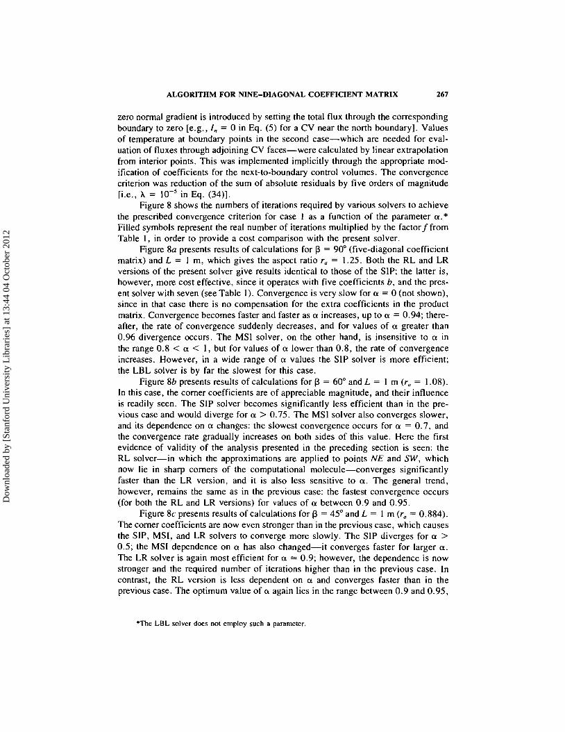
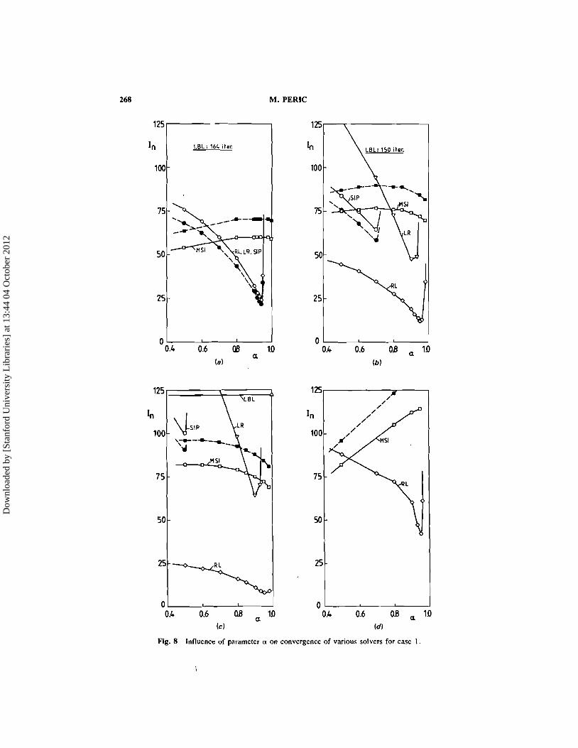
Figure 8 shows the numbers of iterations required by various solvers to achieve the prescribed convergence criterion for case 1 as a function of the parameter a.* Filled symbols represent the real number of iterations multiplied by the factor f from Table I, in order to provide a cost comparison with the present solver.
Figure 8a presents results of calculations for P = 90" (five-diagonal coefficient matrix) and L = 1 m, which gives the aspect ratio r. = 1.25. Both the RL and LR versions of the present solver give results identical to those of the SIP; the latter is, however, more cost effective, since it operates with five coefficients b, and the pres- ent solver with seven (see Table 1). Convergence is very slow for a = 0 (not shown), since in that case there is no compensation for the extra coefficients in the product matrix. Convergence becomes faster and faster as a increases, up to a = 0.94; there- after, the rate of convergence suddenly decreases, and for values of a greater than 0.96 divergence occurs. The MSI solver, on the other hand, is insensitive to a in the range 0.8 < a < 1, but for values of a lower than 0.8, the rate of convergence increases. However, in a wide range of a values the SIP solver is more efficient; the LBL solver is by far the slowest for this case.
Figure 8b presents results of calculations for P = 60" and L = 1 m (r,, = 1.08). In this case, the comer coefficients are of appreciable magnitude, and their influence is readily seen. The SIP solver becomes significantly less efficient than in the pre- vious case and would diverge for a > 0.75. The MSI solver also converges slower, and its dependence on a changes: the slowest convergence occurs for a = 0.7, and the convergence rate gradually increases on both sides of this value. Here the first evidence of validity of the analysis presented in the preceding section is seen: the RL solver-in which the approximations are applied to points NE and SW, which now lie in sharp comers of the computational molecule-converges significantly faster than the LR version, and it is also less sensitive to a. The general trend, however, remains the same as in the previous case: the fastest convergence occurs (for both the RL and LR versions) for values of a between 0.9 and 0.95.
Figure 8c presents results of calculations for P = 45" and L = 1 m (r, = 0.884). The comer coefficients are now even stronger than in the previous case, which causes the SIP, MSI, and LR solvers to converge more slowly. The SIP diverges for a > 0.5; the MSI dependence on a has also changed-it converges faster for larger a. The LR solver is again most efficient for a = 0.9; however, the dependence is now stronger and the required number of iterations higher than in the previous case. In contrast, the RL version is less dependent on a and converges faster than in the previous case. The optimum value of a again lies in the range between 0.9 and 0.95,
*The LBL solver does not employ such a parameter
Dow
nloa
ded
by [
Stan
ford
Uni
vers
ity L
ibra
ries
] at
13:
44 0
4 O
ctob
er 2
012
LBL: 16L iter
100
Fig. 8 Influence of parameter a on convergence of various solvers for case I
\
Dow
nloa
ded
by [
Stan
ford
Uni
vers
ity L
ibra
ries
] at
13:
44 0
4 O
ctob
er 2
012
ALGORITHM FOR NINE-DIAGONAL COEFFICIENT MATRIX 269
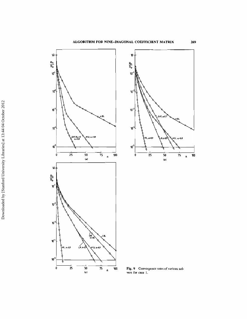
Fig. 9 Convergence rates of various sol- IcI vers for case 1
Dow
nloa
ded
by [
Stan
ford
Uni
vers
ity L
ibra
ries
] at
13:
44 0
4 O
ctob
er 2
012

Fig. 10 Influence o f parameter a on convergence of various solvers for case 2.
but even for a = 0 the RL solver is about three times more efficient than the best competitor, the MSI.
Calculations were also performed for P = 120" and 135". In this case the LR and RL solvers interchange role: the LR converges for P = 135" in exactly the same way as the RL for P = 45". This is further proof that the "propern arrangement of vector {+} (LR for P > 90" and RL for P < 90") does lead to faster convergence.
To check the influence of aspect ratio r, on the rate of convergence, calcula- tions were also performed for P = 45" and L = 10 m (r,, = 8.84, but L / H = 12.5). Figure 8d presents a comparison of the performance of the RL and MSI solvers as a function of a. Both solvers now show a strong dependence on a; the MSI converges faster as a decreases (contrary to the previous case), while the RL behaves in the usual way, being most efficient for a between 0.9 and 0.96. Comparison with Fig. 8c reveals, however, that values of the aspect ratio significantly greater than unity adversely affect the rate of convergence of the present solver. This is presumably due to the disproportion in magnitudes of coefficients of matrix [A] in the I' and x2 directions (the coefficients a, and a, are about r, times greater than the coefficients a, and a,).
Figures 90-9c show the variation of the sum of absolute residuals as a function of the number of iterations performed for case I (L = I m and P = 90'. 60°, and 4S0, respectively). It is interesting that the slope of these curves (logarithmic scale in one direction) remains constant for all solvers in a certain range of residual levels; it then changes and stays constant again for another range. For P = 60" and 45" the
Dow
nloa
ded
by [
Stan
ford
Uni
vers
ity L
ibra
ries
] at
13:
44 0
4 O
ctob
er 2
012

ALGORITHM FOR NINE-DIAGONAL COEFFICIENT MATRIX 27 1
MSI shows one more "turning" region than the LR and RL; moreover, in both cases the curves for LR and MSI almost coincide until about R,/R, = 5 X after which the MSI becomes slower. These diagrams clearly demonstrate the efficiency of the RL solver for these cases.*
In all variants of case I, a uniform grid (20 x 20 CV) was used, with r,, and p constant over the domain. In practical situations where nonorthogonal grids are used, usually both the aspect ratio and the angle P vary from one control volume to another. Case 2, therefore, represents a test case that is much closer to reality; here the aspect ratio ranges between 1 and 8 and the angle P between 45" and 135". However, in most of the solution domain p is less than 90°, which is why the RL solver was expected to give better results.
Figure 10 shows results of calculations for case 2. The MSI procedure con- verges faster for lower values of a; the SIP diverges for a > 0.75 and is significantly slower than the MSI. The RL solver shows its typical dependence on a; the fastest convergence occurs for values between 0.9 and 0.95. In this range it is significantly more efficient than any of the other solvers tried, especially in terms of computing time.
Solution of Pressure-Correction Equation
As already noted, the pressure-correction equation, which results from the SIMPLE and similar algorithms for the velocity-pressure coupling 19-1 I], is basi- cally of the same type as the diffusion equation [Eq. (I)]. When nonorthogonal grids are used to solve the fluid flow equations, a nine-coefficient pressure-correction equation
4 0.6 0.8 1 .O 0.4 0.6 0.8 a a
1 .o la) ( b )
Fig. 11 Influence of parameter a on convergence of various solvers for case 3.
*Note that the resulrs are shown (for RL, LR, and MSI) for a = 0.9, which is not the optimum value for the RL solver.
Dow
nloa
ded
by [
Stan
ford
Uni
vers
ity L
ibra
ries
] at
13:
44 0
4 O
ctob
er 2
012

Fig. I2 Influence of parameter a on convergence of various solvers for case 4 and 20 x 20 CV grid.
of the form of Eq. (6) results (e.g., see [3]). However, i t usually converges slower than the typical diffusion equation for the following reasons: ( I ) the coefficient cor- responding to r+ of Eq. ( I ) varies from one control volume to another, (2) the source term (mass imbalance) varies from one control volume to another, and (3) the bound- ary conditions are typically of the Neuman type for all boundaries (zero normal gradient). As the convergence criterion, a value of A between 0.1 and 0.25 is usually used 19, 1 I ] .
Dow
nloa
ded
by [
Stan
ford
Uni
vers
ity L
ibra
ries
] at
13:
44 0
4 O
ctob
er 2
012
ALGORITHM FOR NINE-DIAGONAL COEFFICIENT MATRIX 273
Since most of the computing time in fluid flow predictions is spent on solving the pressure-correction equation, it is important to have an efficient solver for it. The usual solvers (like LBL and SIP) have proved inefficient in the case of a full nine-point pressure-correction equation, which is why, in most flow prediction pro- cedures for nonorthogonal grids, a simplified version of the pressure-correction equa- tion with a five-diagonal coefficient matrix is used [3-61. This, however, slows down the overall convergence when the grid nonorthogonality is appreciable [3].
In order to test the performance of various solvers when solving the pressure- correction equation with a nine-diagonal coefficient matrix, calculations were per- formed for cases 3 and 4 described above.
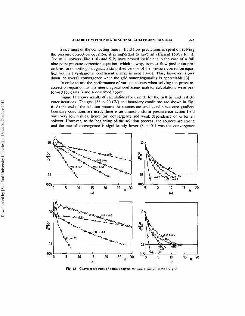
Figure I I shows results of calculations for case 3, for the first (a) and last (b) outer iterations. The grid (33 X 20 CV) and boundary conditions are shown in Fig. 6. At the end of the solution process the sources are small, and since zero-gradient boundary conditions are used, there is an almost uniform pressure-correction field with very low values, hence fast convergence and weak dependence on a for all solvers. However, at the beginning of the solution process, the sources are strong and the rate of convergence is significantly lower (A = 0. I was the convergence
Fig. 13 Convergence rates of various solvers for case 4 and 20 X 20 CV grid.
Dow
nloa
ded
by [
Stan
ford
Uni
vers
ity L
ibra
ries
] at
13:
44 0
4 O
ctob
er 2
012
criterion for all calculations with the pressure-correction equation). The dependence of performance on a is similar to that seen for case 2 (see Fig. 1 l a and Fig. 10); only the MSI solver now shows a somewhat weaker dependence on a. The RL solver again converges fastest for a between 0.9 and 0.96, and it is significantly more efficient than the nearest competitor, the MSI.
Figure 12 presents results of calculations for case 4 on a 20 x 20 CV grid and for two angles of inclination: P = 63" (Figs. 12a and 12b, for the first and the last outer iteration) and p = 45' (Figs. 12c and 12d, as above). For P = 63" the SIP solver converges for values of a up to 0.75; however, for P = 4S0, where the comer coefficients are stronger, it converges-but slower-for values of a only up to 0.5.
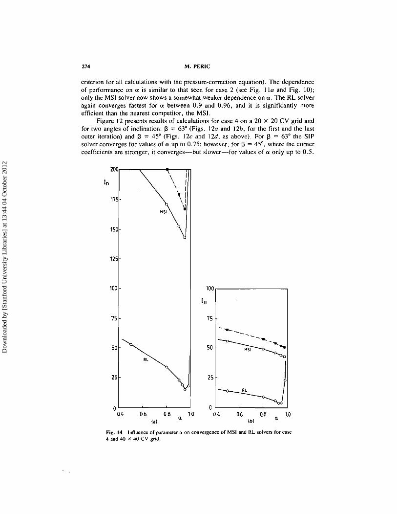
Fig. 14 Influence of parameter a on convergence of MSI and RL solvers for case 4 and 40 X 40 CV grid.
Dow
nloa
ded
by [
Stan
ford
Uni
vers
ity L
ibra
ries
] at
13:
44 0
4 O
ctob
er 2
012
ALGORITHM FOR NINE-DIAGONAL COEFFICIENT MATRIX
( b )
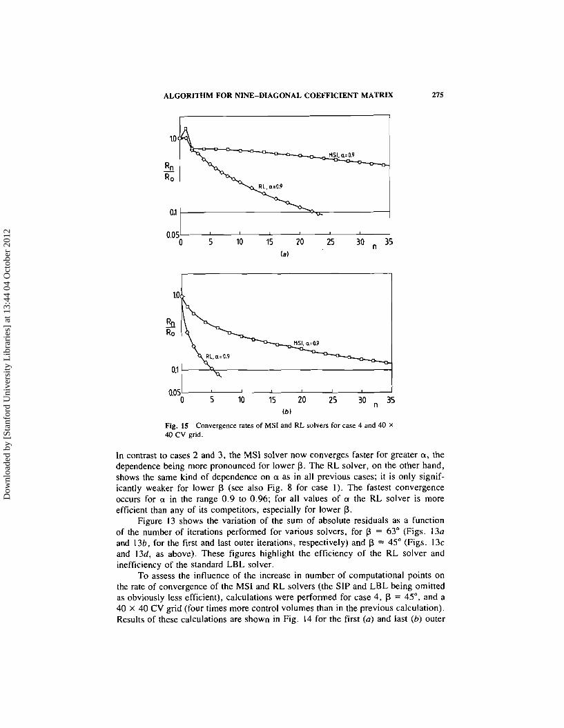
Fig. 15 Convergence rates of M S I and RL solvers for case 4 and 40 X
40 CV grid.
In contrast to cases 2 and 3, the MS1 solver now converges faster for greater a, the dependence being more pronounced for lower P. The RL solver, on the other hand, shows the same kind of dependence on a as in all previous cases; it is only signif- icantly weaker for lower P (see also Fig. 8 for case 1). The fastest convergence occurs for a in the range 0.9 to 0.96; for all values of a the RL solver is more efficient than any of its competitors, especially for lower P.
Figure 13 shows the variation of the sum of absolute residuals as a function of the number of iterations performed for various solvers, for P = 63" (Figs. 13a and 136, for the tirst and last outer iterations, respectively) and P = 45" (Figs. 13c and 13d, as above). These figures highlight the efficiency of the RL solver and inefficiency of the standard LBL solver.
To assess the influence of the increase in number of computational points on the rate of convergence of the MSI and KL solvers (the SIP and LBL being omitted as obviously less efficient), calculations were performed for case 4, P = 45". and a 40 X 40 CV grid (four times more control volumes than in the previous calculation). Results of these calculations are shown in Fig. 14 for the first (a) and last (b) outer
Dow
nloa
ded
by [
Stan
ford
Uni
vers
ity L
ibra
ries
] at
13:
44 0
4 O
ctob
er 2
012

iterations. Comparisons with Figs. 12c and l2d, which show the corresponding re- sults for the 20 X 20 CV grid, reveal that both solvers become more sensitive to the value of a and converge slower when the number of computational points in- creases. The MSI appears to be more sensitive: for a 20 X 20 CV grid and a = 0.9, the ratio of the number of iterations required by the MSI and R L solvers to achieve the same level of convergence was about 4.5 (first outer iteration) to 3.5 (last outer iteration), while for a 40 X 40 CV grid this ratio ranged between 6.6 and 7.8. In other words, for a fourfold increase in the number of computational points, the num- ber of iterations increased about six times for the MSI and four times for the RL solver.
Figure 15 shows the variation of the sum of absolute residuals as a function of the number of iterations performed for the above case.. At the beginning of the solution process (Fig. 15a) both MSI and RL show an increase in residuals after the first iteration; after the second iteration, both solvers show the same level of resid- uals, but thereafter the rate of reduction is much faster for the RL. At the end of solution process (Fig. 15b) the variation is smooth for both solvers; the reduction is, however, much faster for the RL solver.
CONCLUSIONS
A new procedure for solving the systems of algebraic equations resulting from the finite-volume (or finite-difference) discretization of conservation equations on nonorthogonal two-dimensional numerical grids is presented. These systems of equa- tions have a nine-diagonal coefficient matrix, and the motivation for the present work was to extend the SIP methodology of Stone [ I ] to accommodate such matrices at the lowest possible increase in computer storage and run time requirements. A mod- erate increase in storage is achieved by using triangular matrices with seven nonzero coefficient diagonals, which is two more than in the SIP but two less than in alter- native extensions to nine-diagonal matrices [12, 131. The computing time per iter- ation in the proposed solver is about 10% higher than in the SIP, but about 16.5% lower than in the alternative (MSI) solver. The new algorithm reduces to that of Stone [ I ] when the coefficient matrix is five-diagonal.
To examine the cost effectiveness of the new solver and the influence of various parameters on the rate of convergence, a series of test calculations was performed. Some involved solution of the diffusion equation to a tight tolerance for mixed boundary conditions and various grid nonorthogonality and aspect ratios. Special attention was paid to the solution of the pressure-correction equation for fluid flow predictions on nonorthogonal grids, since it is particularly difficult to solve and therefore could yield the greatest computing time savings. From the results of these calculations and com- parisons with three alternative solution methods (the SIP of Stone [I], the MSI of Schneider and Zedan 1131, and the standard LBL method[lO]) the following con- clusions can be made:
I . For the kind of equations and discretization practices studied, the newly proposed solver is particularly efficient when the matrices are arranged so that the points in sharp corners of the computational molecule need approximations of the kind given by Eq. (16). This is explained'by analyzing the errors in the two-step approximation procedure and confirmed by all test calculations.
Dow
nloa
ded
by [
Stan
ford
Uni
vers
ity L
ibra
ries
] at
13:
44 0
4 O
ctob
er 2
012

ALGORITHM FOR NINE-DIAGONAL COEFFICIENT MATRIX 277
2. The dependence of the new solver on the cancellation parameter a, shows a regular pattern, and in all cases studied here the optimum value lay in the range 0.9 to 0.95. The SIP solver shows the same kind of dependence, but the optimum value is reduced and the convergence rate decreases when the comer coefficients become stronger. The dependence of the MSI procedure on a varies from case to case and a typical optimum range cannot be identified, at least not for the cases studied here.
3. Departure of the grid aspect ratio from unity increases the sensitivity of the proposed solver to a; the optimum range, however, remains the same.
4. Increasing grid nonorthogonality for the kind of equations studied here re- sults in reduced sensitivity of the proposed solver to the parameter a, and an increase in the convergence rate; for other solvers tried the opposite is true.
5. The proposed solver is less sensitive to an increase in the number of com- putational points than the best alternative tried, the MSI (at least for the case tested).
6. For a, values in the range mentioned above and all cases tested, the proposed solver is more efficient than the other methods tried. In cases of strong grid non- orthogonality and aspect ratio close to unity, it required up to seven times fewer iterations (up to eight times less computing time) to reach the prescribed convergence limit than the most efficient alternative. the MSI method.
These conclusions are valid for application of the solvers tested to equations resulting from the nine-point discretization of the differential conservation equations on nonorthogonal grids, as indicated in the Introduction. The errors introduced by approximations in the two steps of the proposed solution algorithm partially cancel when the matrices are arranged in an appropriate way, giving a significant increase in the rate of convergence. Although the proposed solver can be applied to any nine- diagonal coefficient matrix of the form studied, the efficiency may not be the same if the coefficients are generated by an operator different from that used in this study.
APPENDIX: BASIC STEPS FOR THE RL ARRANGEMENT
When the vector {+} is arranged in the RL fashion (index j changing from I to N, and index i backward from N , to I), then the coefficients in matrix [A] cor- responding to the SE, E , NE points interchange places on the nonzero diagonals with those corresponding to the SW, W, and NW points, as compared to the LR arrange- ment shown in Fig. 3. The missing diagonals in the [L] and [U] matrices now cor- respond to the NE and SW points.-The coefficients of the product matrix [C] can then be expressed in terms of the coefficients b of the [I,] and [U] matrices as fol- lows:
Dow
nloa
ded
by [
Stan
ford
Uni
vers
ity L
ibra
ries
] at
13:
44 0
4 O
ctob
er 2
012

Now points NE and SW require special treatment, and approximations of the follow- ing form can be applied [see Eq. (16)l:
Steps I and 2 are analogous to those presented for the LR arrangement and lead to the following expressions for the coefficients b:
The iteration procedure follows in the same way as for the LR arrangement. The formulas equivalent to Eqs. (31) and (32) now read
REFERENCES I . H . L. Stone, Iterative Solution of Implicit Approximations of Multidimensional Partial
Differential Equations, SIAM J. Numer. Anal., vol. 5, Pp. 530-558, 1968.
Dow
nloa
ded
by [
Stan
ford
Uni
vers
ity L
ibra
ries
] at
13:
44 0
4 O
ctob
er 2
012

ALGORITHM FOR NINE-DIAGONAL COEFFICIENT MATRIX 279
2. S . B. Pope, The Calculation of Turbulent Recirculating Flows in General Orthogonal Coordinates, J. Comput. Phys., vol. 22, pp. 197-217, 1978.
3. 1. A. Demirdzic, A Finite Volume Method for Computation of Fluid Flow in Complex Geometries, Ph.D. thesis, University of London, 1982.
4. 1. Demirdzic. A. D. Gosman, R. I. Issa, and M. Peric, A Calculation Procedure for Turbulent Flow in Complex Geometries, Fluids Section Rept. FS/85/39, Mechanical Engineering Dept., Imperial College, London, 1985.
5. C. M. Rhie and W. L. Chow, A Numerical Study of the Turbulent Flow Past an Isolated Airfoil with Trailing Edge Separation, AIAA-82-0998, 1982.
6. C . Hah, A Navier-Stokes Analysis of Three-Dimensional Turbulent Flows inside Turbine Blade Rows at Design and Off-Design Conditions, ASME 83-GT-40, 1983.
7. 1. Demirdzic, A. D. Gosman, and R. I. Issa, A Finite-Volume Method for the Prediction of Turbulent Flow in Arbitrary Geometries in Proceedings of the 7th Internutionul Con- Jerence on Numerical Methods in Fluid Dynamics, Stanford, pp. 144- 150, Springer Ver- lag, New York, 1980.
8. G. D. Raithby and G. E. Schneider, Numerical Solution of Problems in Incompressible Fluid Flow: Treatment of the Velocity-Pressure Coupling, Numer. Heat Transfer, vol. 2, pp. 417-440. 1979.
9. J. P. Van Doormal and G. D. Raithby, Enhancement of ihe SIMPLE Method for Pre- dicting Incompressible Fluid Flows, Numer. Heat Transfer, vol. 7 , pp. 147-163, 1984.
10. S. V. Patankar, Numerical Heat Transfer and Fluid Flow. Hemisphere, Washington. D.C., 1980.
I I . R. I. Issa, Solution of the Implicitly Discretized Fluid Flow Equations by Operator-Split- ting, J. Camp. Phys., vol. 62, pp. 40-65, 1985.
12. D. A. H. Jacobs, A Subroutine for Iterating Using a Nine Diagonal Matrix to Solve a System of Algebraic Equations, CERL Note RD/L/P15/79, Central Electricity Research Laboratories, Leatherhead, Surrey, England, 1980.
13. G. E. Schneider and M. Zedan, A Modified Strongly Implicit Procedure for the Nu- merical Solution of Field Problems, Numer. Hear Transfer, vol. 4 , pp. 1-19, 1981.
Received January 31. 1986 Accepted August 26. 1986
Dow
nloa
ded
by [
Stan
ford
Uni
vers
ity L
ibra
ries
] at
13:
44 0
4 O
ctob
er 2
012