Efficient techniques for risk assessment of space frame

HSEHealth & Safety

Executive

Efficient techniques for risk assessment ofspace frame platforms exposed to random

wave and current loading

Some thoughts on extension to cover effects ofintermittency and directionality

Prepared by theUniversity of Liverpool

for the Health and Safety Executive

OFFSHORE TECHNOLOGY REPORT

2002/011

HSEHealth & Safety

Executive

Efficient techniques for risk assessment ofspace frame platforms exposed to random

wave and current loading

Some thoughts on extension to cover effects ofintermittency and directionality

G Najafian, R Burrows & R G TickellDepartment of Civil Engineering

University of LiverpoolLiverpoolL69 3GQ

United Kingdom

HSE BOOKS

ii

© Crown copyright 2002Applications for reproduction should be made in writing to:Copyright Unit, Her Majesty’s Stationery Office,St Clements House, 2-16 Colegate, Norwich NR3 1BQ

First published 2002

ISBN 0 7176 2342 4

All rights reserved. No part of this publication may bereproduced, stored in a retrieval system, or transmittedin any form or by any means (electronic, mechanical,photocopying, recording or otherwise) without the priorwritten permission of the copyright owner.

This report is made available by the Health and SafetyExecutive as part of a series of reports of work which hasbeen supported by funds provided by the Executive.Neither the Executive, nor the contractors concernedassume any liability for the reports nor do theynecessarily reflect the views or policy of the Executive.

iii

EXECUTIVE SUMMARY Offshore structures are subject to a wide variety of environmental loads (such as wind, wave and current) all of which exhibit a high degree of statistical uncertainty. The structural components, e.g., beams, columns, connections, piles, conductors and risers, must be proportioned to resist the effects of these loads. Uncertainties in capacities or member strengths arise because of material and fabrication variability and limitations in engineering theories to predict and conveniently interpret element and system response and capacity. As a result, a reliability-based approach is necessary to account for these uncertainties. One of the most important uncertainties arises in the prediction of the probability distribution of the extreme values of response (during a given period of exposure) due to wave and current loading. The major obstacle in the probabilistic analysis of wave and current effects, is the nonlinearity of the drag component of Morison's wave loading which results in non-Gaussian probability distributions for both loading and response. The problem is further compounded in the free surface zone due to load intermittency. The dynamic response of offshore structures is usually closer to a Gaussian distribution than that of quasi-static response, especially for structures with low damping ratios. However, extensive Monte Carlo simulations have shown that the dynamic responses of drag-dominated structures such as jacket platforms are distinctly non-Gaussian. Extensive time-domain simulation can be used to establish the probability distribution of response extreme values with good accuracy. However, given that the probability of failure of a structure during its service time requires the evaluation of response extreme values for many different combinations of significant waveheight, mean zero-crossing period, predominant wave direction, current, etc., extensive time domain simulation becomes impracticable. Consequently, the reliability analysis of the structure must be based on insufficiently long simulations, which leads to insufficiently accurate results due to significant sampling variability, or alternatively, on insufficiently accurate extreme value probability models (such as assuming that the response is Gaussian), which leads to potentially large systematic errors. In either case, the high level of uncertainty will lead to a high notional probability of failure for the structure. On the other hand, the uncertainty in the predicted values of response extremes, when determined from an accurate model, would be small, leading to a much lower notional probability of failure for the structure. It is beneficial, therefore, to develop accurate and efficient techniques for prediction of response extreme values for both quasi-static and dynamic structures. The successful outcome of a recent two-year EPSRC research study was to develop efficient but accurate techniques for the prediction of the probability distribution of the extreme values of response experienced by (linear) jacket structures exposed to random Morison wave loading under stationary sea-states. This resulted in the development of: a Factor Analysis Technique, as a more computationally efficient alternative to time simulation; a Dynamic Excess Kurtosis technique to estimate the scale of non-Gaussianity of the response for dynamic structures; and Najafian’s Extreme Value probability model (NEV) to provide representation of the extremal statistics. The current project has aimed to extend applicability of these methods. The specific objectives were:- to incorporate the effect of current and load intermittency in the splash zone into the NEV probability modelling approach; and also to extend the techniques for efficient evaluation of kurtosis (a crucial parameter in the characterisation of a probability distribution) to cases when current, load intermittency and wave directionality are important. The principal achievements from the study can be summarised as follows: • A robust implementation of the time simulation technique, directed towards the reliable

estimation of extreme values of response has been successfully extended to account for current and load intermittency in the splash zone.

• The Factor Analysis technique has been extended to account for current, wave directionality and load intermittency in the splash zone. The results of this technique have been compared

iv

against those from time simulation technique to confirm both its accuracy and its much higher computational efficiency (about 25 times for long-crested seas and at least 100 times for directional seas).

• The effects of current and load intermittency on the statistical properties of both dynamic and quasi-static responses have been thoroughly investigated.

• Extension of the Dynamic Excess Kurtosis Technique and Najafian’s Extreme Value probability model to the case of structures under the influence of load intermittency and current has been thoroughly investigated. Extensive investigation has shown that the Pierson-Holmes distribution can accurately account for the effect of current on the probability distribution of response. However, it cannot accurately model the effect of the load intermittency in the splash zone on the response probability distribution.

• A methodology for establishing an improved probability model for the response distribution arising from structures subject to load intermittency has been devised. The proposed methodology can also be used to determine the probabilistic properties of the dynamic response from those of the quasi-static response.

v

TABLE OF CONTENTS

Page No.

EXECUTIVE SUMMARY iii

1. BACKGROUND 1 2. THE EFFECT OF CURRENT ON THE WAVE FREQUENCY SPECTRUM 2 3. EVALUATION OF WAVE KINEMATICS IN THE FREE SURFACE ZONE 2 4. ACCOUNTING FOR LOAD INTERMITTENCY IN THE SPLASH ZONE 2 5. TEST STRUCTURES 2 6. TIME SIMULATION PROCEDURE FOR GENERATING EXTREME VALUES AND

OTHER STATISTICAL PROPERTIES OF RESPONSE 3 7. FACTOR ANALYSIS PROCEDURE FOR GENERATING EXTREME VALUES AND

OTHER STATISTICAL PROPERTIES OF RESPONSE 4 8. EXTENSION OF THE TIME SIMULATION AND FACTOR ANALYSIS PROCEDURES

TO ACCOUNT FOR WAVE DIRECTIONALTY 5 9. COMPARISON OF RESPONSE STATISTICS FROM TIME SIMULATION AND

FACTOR ANALYSIS PROCEDURES 7 10. EFFICIENCY OF THE FACTOR ANALYSIS PROCEDURE IN COMPARISON WITH

THE TIME SIMULATION PROCEDURE 7 11. PERFORMANCE OF PIERSON-HOLMES DISTRIBUTION IN MODELLING THE

PROBABILITY DISTRIBUTION OF QUASI-STATIC AND DYNAMIC RESPONSES 8 12. THE EFFECT OF LOAD INTERMITTENCY ON THE PROBABILITY

DISTRIBUTIONS OF THE RESPONSE AND ITS EXTREME VALUES 9 13. DYNAMIC EXCESS KURTOSIS TECHNIQUE 9 14. METHODOLOGY FOR IMPROVING ON THE DYNAMIC EXCESS KURTOSIS

TECHNIQUE AND ESTABLISHING AN ALTERNATIVE TO PIERSON-HOLMES DISTRIBUTION, TO BETTER ACCOUNT FOR LOAD INTERMITTENCY IN THE SPLASH ZONE 10

15. CLOSURE 11 ACKNOWLEDGEMENTS 11

REFERENCES 11

vi

APPENDIX A: THE EFFECT OF CURRENT ON THE FREQUENCY SPECTRUM 45 APPENDIX B: LOAD INTERMITTENCY IN THE SPLASH ZONE 55 APPENDIX C: CROSS-COVARIANCE MATRIX OF WATER PARTICLE KINEMATICS 56

1

1 - BACKGROUND Offshore structures are subject to a wide variety of environmental loads (such as wind, wave and current) all of which exhibit a high degree of statistical uncertainty. The structural components, e.g., beams, columns, connections, piles, conductors and risers, must be proportioned to resist the effects of these loads. Uncertainties in capacities or member strengths arise because of material and fabrication variability and limitations in engineering theories to predict and conveniently interpret element and system response and capacity. As a result, a reliability-based approach is necessary to account for these uncertainties. One of the most important uncertainties arises in the prediction of the probability distribution of the extreme values of response (during a given period of exposure) due to wave and current loading. The major obstacle in the probabilistic analysis of wave and current effects, is the nonlinearity of the drag component of Morison's wave loading which results in non-Gaussian probability distributions for both loading and response. The problem is further compounded by the members in the free surface zone due to load intermittency. The dynamic response of offshore structures is usually closer to a Gaussian distribution than that of quasi-static response, especially for structures with low damping ratios. However, extensive Monte Carlo simulations have shown that the dynamic responses of drag-dominated structures such as jacket platforms are distinctly non-Gaussian (Karunakaran et al., 1992). Extensive time-domain simulation can be used to establish the probability distribution of response extreme values with good accuracy. However, given that the probability of failure of a structure during its service time requires the evaluation of response extreme values for many different combinations of significant waveheight, mean zero-crossing period, predominant wave direction, current, etc., extensive time domain simulation becomes impracticable. Consequently, the reliability analysis of the structure must be based on insufficiently long simulations, which leads to insufficiently accurate results due to significant sampling variability, or alternatively, on insufficiently accurate extreme value probability models (such as assuming that the response is Gaussian), which leads to potentially large systematic errors. In either case, the high level of uncertainty will lead to a high notional probability of failure for the structure (Ditlevsen and Madsen, 1996). On the other hand, the uncertainty in the predicted values of response extremes, when determined from an accurate model, would be small, leading to a much lower notional probability of failure for the structure (Ditlevsen and Madsen, 1996). It is therefore beneficial to develop accurate and efficient techniques for prediction of response extreme values for both quasi-static and dynamic structures. The objective of a recent two-year EPSRC research study (Burrows, Najafian, Tickell, Hearn and Metcalfe, 2001), which led to the current project, was to develop efficient but accurate techniques for the prediction of the probability distribution of the response extreme values for a (linear) jacket structure exposed to random Morison wave loading due to a (stationary) sea-state. The study led to the development of the following procedure:

i. The computationally efficient Factor Analysis Technique (Najafian et al, 2002) was developed to simulate statistically independent values of the quasi-static response. The simulated data can be used to accurately estimate the first four statistical moments (mean, standard deviation, skewness and kurtosis) of quasi-static response. This is a substantial improvement over standard time simulation approaches.

ii. For cases when dynamic effects are important, the Dynamic Excess Kurtosis Technique was developed to calculate the kurtosis of dynamic response from their corresponding quasi-static values.

iii. Use the first four statistical moments of response to calculate the theoretical probability distribution of response by assuming that it is Pierson-Holmes (P-H) distributed (Najafian et al, 2000).

2

iv. Use Najafian’s Extreme Value (NEV) probability model (which is based on the assumption that the response itself is P-H distributed) to establish the theoretical probability distribution of response extreme values during a given period of exposure.

These techniques were tested by exposing a test structure to sea-states of varying intensity and proved to be both efficient and accurate. However, due to time restrictions, the effect of current, load intermittency in the splash zone and wave directionality were not incorporated in the developed models. The purpose of the current project reported here was to carry out further work to investigate the effect of current and load intermittency on the probabilistic properties of the response and its extreme values and to extend the foregoing procedure to cases when current, load intermittency and wave directionality are important. In particular, it was intended • to extend the Factor Analysis Technique to account for current, load intermittency in the

splash zone and wave directionality. • to establish whether the Dynamic Excess Kurtosis Technique leads to sufficiently accurate

estimates of dynamic response kurtosis. • to establish whether Pierson-Holmes and Najafian’s Extreme Value probability distributions

are good models for the distribution of response and its extreme values, respectively. • to introduce alternative methodology for establishing accurate probability models for the

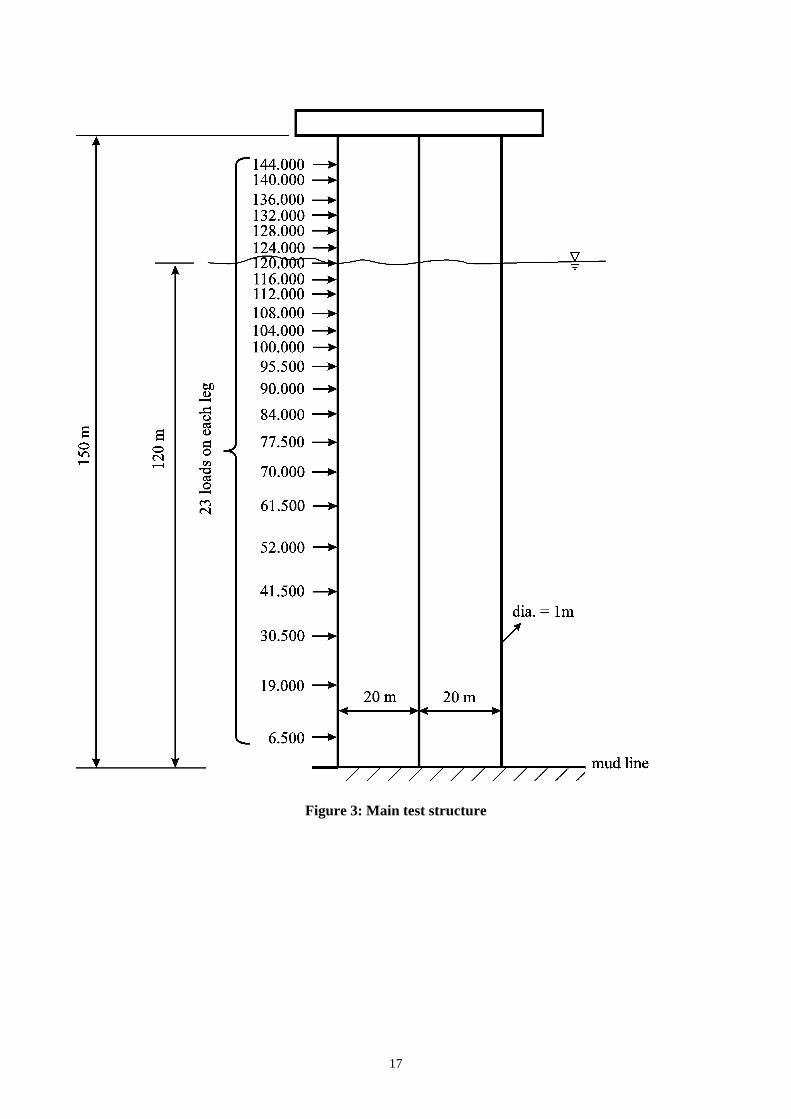
response and its extreme values in case the foregoing models are not sufficiently accurate. 2 - THE EFFECT OF CURRENT ON THE WAVE FREQUENCY SPECTRUM Both positive and negative currents have been considered in this project (a current is considered to be positive if it is in the direction of wave propagation). The surface elevation frequency spectrum in the frame of reference moving with the current would be different from that in a stationary frame of reference because the speed of the wave propagation in the two frames of reference would be different. In this project, the frequency spectrum in the frame of reference moving with the current is assumed to be a Pierson-Moskowitz spectrum defined by its significant wave height. This will then be modified to define the frequency spectrum for the stationary observer, i.e. the structure. The related issues are discussed in Hedges et al (1979), Hedges (1987), Hedges and Lee (1992) and Hedges and Akrigg (1993) and are given in Appendix A for completeness. The effects of both positive and negative currents on the surface elevation frequency spectrum are demonstrated in Figures 1 and 2, respectively. 3 - EVALUATION OF WAVE KINEMATICS IN THE FREE SURFACE ZONE A common industry practice consists of using linear wave theory in conjunction with empirical wave stretching techniques to provide a more realistic representation of near-surface water kinematics. The empirical wave stretching techniques popular in the offshore industry include vertical stretching, linear extrapolation, Wheeler stretching and delta stretching (Couch and Conte, 1997). Vertical stretching (Marshall and Inglis, 1986) is computationally more efficient and hence was adopted for this study. 4 - ACCOUNTING FOR LOAD INTERMITTENCY IN THE SPLASH ZONE A Heavyside function was used to account for load intermittency in the splash zone. The details are given in Appendix B. 5 - TEST STRUCTURES The main test structure, used in this report, is a simple two-dimensional structure in a water depth of 120m, as shown in Figure. 3. It is composed of three 1.00m diameter vertical legs with 23 nodal loads representing the distributed load on each leg. The distance between any two

3

adjacent legs is 20m. The total number of loads was considered to be 69, so that the statistical properties of response such as its kurtosis or extreme value probability distribution can be calculated accurately by extensive time simulation without excessive computer run-time demand. It should be noted that the foregoing structure is fictitious and is meant to easily provide a relatively large number of nodal loads with some spatial (horizontal and vertical) separation. In order to investigate the effect of water depth on probabilistic properties of response, a second test structure was introduced. The test structure, shown in Figure 4, is similar to the first test structure except that the water depth has increased to 250m and the number of nodes on each leg has increased to 33. Unless otherwise specified all the results in this report refer to the main test structure, shown in Figure 3. The structure was subjected to various uni-directional Pierson-Moskowitz sea-states (as measured by the observer moving with the current) defined by their associated significant wave heights (Hs = 15m, 10m and 5m). The current was assumed to vary between ±1.5m/sec and the mean wave zero-upcrossing period (in seconds and for the observer moving with the current) for each sea-state was taken to be sz HT 55.3= . As in Karunakaran et al (1993) and Vugts et al (1998), the two responses chosen for investigation were base shear and overturning moment. For all tests, the member surfaces were assumed to be either smooth or rough. The drag and inertia coefficients for the case of smooth cylinders were assumed to be 0.70 and 1.70, and for the case of rough cylinders were taken to be 1.3 and 1.5, respectively. For the case of dynamic response, the natural frequency of the structural system was assumed to be 0.15 Hz and the equivalent viscous damping (structural + hydrodynamic) ratio was assumed to be 0.03 unless otherwise specified. These values represent a structure with a significant dynamic response, modelled as a single-degree-of-freedom system with no time-varying hydrodynamic damping (fluid-structure interaction). Structures exposed to directional seas have also been considered. As simulation of directional seas are time consuming, a single-column structure, as shown in Figure 5, was chosen for this purpose. The spreading function is defined in Eq. (6) of Section 8 and the spreading parameter was taken to be n = 4 for all frequencies. 6 - TIME SIMULATION PROCEDURE FOR GENERATING EXTREME VALUES

AND OTHER STATISTICAL PROPERTIES OF RESPONSE The steps in this procedure are: (refer to the flowchart in Figure 6) 1. Define the frequency spectrum in the frame of reference moving with the current as a

Pierson-Moskowitz spectrum. 2. Calculate the frequency spectrum for the stationary observer, i.e. the structure (Appendix

A). 3. Simulate surface elevation as a Gaussian process at an arbitrary point from the given

frequency spectrum for a given period of time (e.g. three hours). 4. Calculate water particle kinematics at different nodes from the surface elevation record by

using appropriate transfer functions from linear wave theory and accounting for the presence of current (Hedges, 1987). Then add the current velocity to wave induced water particle velocity.

5. Calculate Morison loads at each node (Morison et al, 1950) accounting for load intermittency in the splash zone.

6. Calculate quasi-static response as a linear combination of nodal loads. If dynamic effects are important, the discrete Fourier transform (DFT) of the dynamic response is determined by multiplying the DFT of the quasi-static response by the frequency response function of the structure. The dynamic response is then determined by taking the Inverse Fourier Transform of its DFT.

4

7. The simulated records can be used to determine statistical properties of response, such as its mean period or its first four statistical moments. Furthermore, both the larger and the smaller extreme values of the generated response record can be determined. It should be noted that the ‘larger’ extreme value is always above the response mean while the ‘smaller’ extreme value is always below the mean. The larger and the smaller extreme values are sometimes referred to as the positive and negative extreme values. This terminology can, however, be misleading as both the larger and the smaller extremes can be positive or negative, depending on the value of the response mean. It is, therefore, preferable to differentiate between the two extremes by designation as the larger and the smaller extreme values.

8. Repeat the process many times to generate a large number of response extreme values and response statistics.

9. The theoretical value of the response statistics can be calculated by assuming that they are equal to the mean of the statistics from all the simulated records. In addition, response extreme values can be plotted on a Gumbel probability paper to compare their distribution against those predicted by different probability models.

According to Linear Random Wave Theory (LRWT), uni-directional seas can be modelled as the sum of a large number of progressive linear waves of different amplitudes travelling in the same direction (positive x axis) with random phases (Borgman, 1969). Then the surface elevation at point x at time t can be modelled as

)(cos),(1

iii

N

ii xktA tx εωη −−= ∑

=

(1)

where ωi are a set of equally-spaced discrete wave frequencies and ki are their associated wavenumbers. εi is the phase angle distributed uniformly in the range 0<εi<2π, and Ai is determined by one of the following two methods: (1) Deterministic Spectrum Amplitude technique (DSA) and (2) Non-Deterministic Spectrum Amplitude (NSA) Technique. That is

2*)()(

)(2)(

22ii

DSAiNSAi

iDSAi

A A

G A

βα

ωωηη

+=

∆=

(2)

where Gηη(ω) is the surface elevation frequency spectrum and ∆ω is the desired frequency interval. αi and βi are two independent standardised Gaussian random variables. Rice (1944, 1945) has shown that when N approaches infinity, the two models will be equivalent to each other. The difference between the two techniques for finite values of N have been discussed in Tucker et al (1984), Grigoriu (1993) and Morooka and Yokoo (1997). As far as the extreme value analysis is concerned, only the NSA technique should be used, especially for short simulations. 7 – FACTOR ANALYSIS PROCEDURE FOR GENERATING EXTREME VALUES

AND OTHER STATISTICAL PROPERTIES OF RESPONSE The steps in this procedure (Najafian et al, 2002) are: (refer to the flowchart in Figure 7) 1. Define the frequency spectrum in the frame of reference moving with the current as a

Pierson-Moskowitz spectrum. 2. Calculate the frequency spectrum for the stationary observer, i.e. the structure. 3. Use linear wave theory to calculate the matrix of cross-covariances between water particle

kinematics and surface elevation at different nodes. 4. Calculate the eigenvalues and eigenvectors of the foregoing matrix. 5. Determine all the important eigenvalues and their associated eigenvectors and ignore the

rest of them.

5

6. Simulate water particle kinematics and surface elevation at each node as a linear combination of important eigenvectors’ components.

7. Calculate Morison loads at each node accounting for load intermittency in the splash zone. 8. Calculate quasi-static response as a linear combination of all the nodal loads. 9. Calculate the statistical properties of quasi-static response such as its first four statistical

moments and its probability distribution. 10. If dynamic effects are important, use the Dynamic Excess Kurtosis Technique to calculate

the statistical properties of dynamic response such as its first four statistical moments. 11. Establish the probability distribution of response extreme values from Najafian’s Extreme

Value probability distribution (Burrows et al, 2001) and compare it with the probability distribution of extreme values from time simulation.

The importance of different eigenvectors for different values of significant waveheight and cylinder roughness condition are shown graphically in Figures 8-10. The eigenvalues have been normalised so that their total sum is equal to unity. These figures indicate that in all cases ten eigenvectors are sufficient. 8 - EXTENSION OF THE TIME SIMULATION AND FACTOR ANALYSIS

PROCEDURES TO ACCOUNT FOR WAVE DIRECTIONALTY Short-crested (directional) seas can be modelled as the sum of a large number of progressive linear waves of different amplitudes travelling in different directions with random phases (Borgman,1969). Let x and y be the coordinates in an arbitrary horizontal Cartesian coordinate system such that the positive y axis is 90 degrees anti-clockwise from the positive x axis. The waves are assumed to travel in a direction θ measured anti-clockwise from the positive x axis. Then the surface elevation at point (x,y) at time t can be modelled as

)]sincos[cos(),,(1 1

ijjji

N

i

M

jiij yxktAtyx εθθωη −+−= ∑∑

= =

(3)

where, as before, ωi are a set of equally-spaced discrete wave frequencies and ki are their associated wave numbers. εij are random phase angles, uniformly distributed in the range [0, 2π]. Aij is the amplitude of the wave with frequency ωi and direction θj. This model is frequently referred to as the double summation model. The directional wave spectrum Gηη(ω,θ) is defined by saying that the wave energy travelling in a small range of frequency ∆ω and a small range of directions ∆θ is G(ω,θ)∆ω∆θ. Then it is standard practice to put Gηη(ω,θ) = Gηη(ω).D(ω,θ), where Gηη(ω) is the point (uni-directional) spectrum and D(ω,θ) represents the angular distribution of energy at frequency ω. The relationship between Aij in the forgoing equation and the directional spectrum is

2*)()(

1),(

),()(

),(.)(2),(2)(

22

max

min

max

min

iiDSAijNSAij

jiijiDSAij

A A

dD

dGG

DGGA

βα

θθω

θθωω

θθωωωθωθω

θ

θ

θ

θηηηη

ηηηη

+=

=

=

∆∆=∆∆=

∫

∫ (4)

6

where, as before, (Aij)DSA and (Aij)NSA refer to the wave amplitude determined from Deterministic Spectrum Amplitude and Non-Deterministic Spectrum Amplitude techniques, respectively, and αi and βi are two independent standardised Gaussian random variables. As was the case for uni-directional seas, only the NSA technique should be used for extreme value analysis, especially for short simulations. The spreading function is defined by (Miles and Funke, 1989)

n

nn

fD

−+Γ

+Γ=

max

0

max 2)(

cos.)2/2/1(2

)2/1(),(

θθθπ

θπ

θ (5)

where Γ is the gamma function and θ0 is the mean (predominant) wave direction and the spreading parameter n may be a function of frequency. θmax is usually set at π/2. Then

( )0cos.

)2/2/1()2/1(

),( θθπ

θ −+Γ

+Γ= n

nn

fD (6)

For simple analysis, where a constant value of n, independent of frequency is used, the value n = 4 is recommended (Barltrop, 1998). The spreading function for n = 4 is shown in Figure 11. The double summation model offers a clear mental picture of the directional seas. However, its application for simulating directional seas is problematic as it leads to seas which are not homogeneous. In other words, the wave energy at a particular frequency can significantly vary from one point to another point (Forristal, 1981 and Pinkster, 1984). In fact, the wave energy in any frequency band can vary over space from approximately 0 to 4 times its average value regardless of how many directions are used (Miles and Funke, 1989). The problem in applying the double summation model is that all the energy in a cell of finite size ∆ω by ∆θ is represented by a single sinusoid. Consequently all the sinusoids with the same frequency travelling at different directions will combine to produce a sinusoidal water surface movement at that frequency, whose amplitude varies from point to point. In real seas this problem does not arise as the frequency band ∆ω is composed of many different frequencies. In other words, the signal in the frequency band ∆ω is a narrow-band random process rather than a sinusoid. Different techniques for simulating directional seas have been discussed by Miles and Funke, 1989 and Yuxiu et al, 1991. The recommended model is the Single Direction per Frequency Model. The Single Direction per Frequency model is defined as

2/2/


ωωωωω

εθθωη

∆+<<∆−

−+−= ∑∑= =

iiji

ijjjij

N

i

M

jijij yxktAtyx

(7)

Therefore, the difference between the double summation model defined in Eq. (3), and the Single Direction per Frequency model is that in the former model, the frequency interval [ωi-∆ω/2, ωi+∆ω/2] is always represented by a single frequency ωi, regardless of the direction θj, while in the latter model, the foregoing interval is represented by a different frequency within the interval for each direction. The Single Direction per Frequency model can efficiently be calculated via FFT if all the ωij are equally spaced. Therefore, in practice, the frequency interval

7

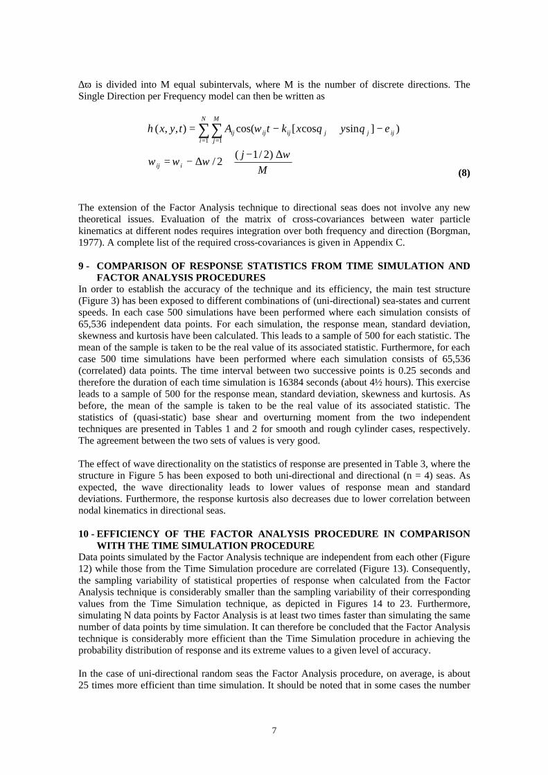
∆ω is divided into M equal subintervals, where M is the number of discrete directions. The Single Direction per Frequency model can then be written as

Mj

yxktAtyx

iij

ijjjij

N

i

M

jijij

ωωωω

εθθωη

∆−+∆−=

−+−= ∑∑= =

)2/1(2/


(8)

The extension of the Factor Analysis technique to directional seas does not involve any new theoretical issues. Evaluation of the matrix of cross-covariances between water particle kinematics at different nodes requires integration over both frequency and direction (Borgman, 1977). A complete list of the required cross-covariances is given in Appendix C. 9 - COMPARISON OF RESPONSE STATISTICS FROM TIME SIMULATION AND

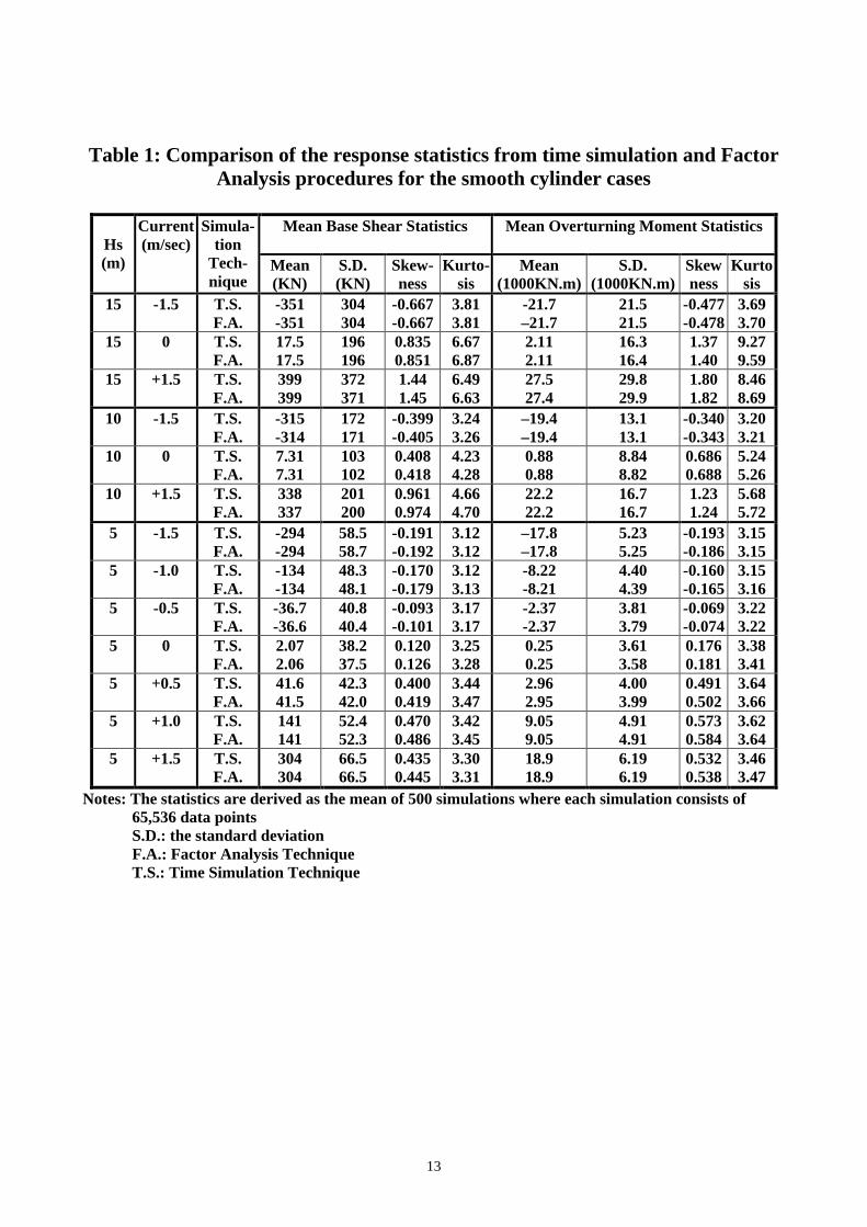
FACTOR ANALYSIS PROCEDURES In order to establish the accuracy of the technique and its efficiency, the main test structure (Figure 3) has been exposed to different combinations of (uni-directional) sea-states and current speeds. In each case 500 simulations have been performed where each simulation consists of 65,536 independent data points. For each simulation, the response mean, standard deviation, skewness and kurtosis have been calculated. This leads to a sample of 500 for each statistic. The mean of the sample is taken to be the real value of its associated statistic. Furthermore, for each case 500 time simulations have been performed where each simulation consists of 65,536 (correlated) data points. The time interval between two successive points is 0.25 seconds and therefore the duration of each time simulation is 16384 seconds (about 4½ hours). This exercise leads to a sample of 500 for the response mean, standard deviation, skewness and kurtosis. As before, the mean of the sample is taken to be the real value of its associated statistic. The statistics of (quasi-static) base shear and overturning moment from the two independent techniques are presented in Tables 1 and 2 for smooth and rough cylinder cases, respectively. The agreement between the two sets of values is very good. The effect of wave directionality on the statistics of response are presented in Table 3, where the structure in Figure 5 has been exposed to both uni-directional and directional (n = 4) seas. As expected, the wave directionality leads to lower values of response mean and standard deviations. Furthermore, the response kurtosis also decreases due to lower correlation between nodal kinematics in directional seas. 10 - EFFICIENCY OF THE FACTOR ANALYSIS PROCEDURE IN COMPARISON

WITH THE TIME SIMULATION PROCEDURE Data points simulated by the Factor Analysis technique are independent from each other (Figure 12) while those from the Time Simulation procedure are correlated (Figure 13). Consequently, the sampling variability of statistical properties of response when calculated from the Factor Analysis technique is considerably smaller than the sampling variability of their corresponding values from the Time Simulation technique, as depicted in Figures 14 to 23. Furthermore, simulating N data points by Factor Analysis is at least two times faster than simulating the same number of data points by time simulation. It can therefore be concluded that the Factor Analysis technique is considerably more efficient than the Time Simulation procedure in achieving the probability distribution of response and its extreme values to a given level of accuracy. In the case of uni-directional random seas the Factor Analysis procedure, on average, is about 25 times more efficient than time simulation. It should be noted that in some cases the number

8

of eigenvectors can be reduced and hence the efficiency can be improved. For example, reducing the number of eigenvectors from 10 to 5 in the case of Hs = 15m has a very small effect on its probability distribution. 11 - PERFORMANCE OF PIERSON-HOLMES DISTRIBUTION IN MODELLING

THE PROBABILITY DISTRIBUTION OF QUASI-STATIC AND DYNAMIC RESPONSE

• The Pierson-Holmes distribution is based on Morison’s equation and is defined as (Najafian et

al, 2000) ( ) 231121 XXXY βγγββ ++++= (9)

where Y is the random variable with Pierson-Holmes distribution, β1, β2, β3 and γ are the four parameters of the distribution 1X and 2X are two Gaussian random variables with the following properties 1;0][][ 2121 ==== XXXEXE σσ (10) • The skewness parameter, γ, models those factors such as current or load intermittency in the

splash zone which give rise to skewness. • The probability distribution of quasi-static overturning moment for a negative and positive

current are shown in Figures 24 and 25, respectively (load intermittency in the splash zone is ignored). It is observed that for these no-intermittency cases the Pierson-Holmes distribution is a very good model for the simulated data.

• The effect of load intermittency on the probability distribution of the response in the

absence of current is demonstrated in Figure 26, where the asymmetry in the probability distribution is clearly shown. It is observed that the simulated data deviates from the theoretical Pierson-Holmes (P-H) distribution. The effect of the asymmetry on the probability distribution of the extreme values is shown in Figure 27, where the magnitude of the larger extreme values are significantly higher than the magnitude of the smaller extreme values.

• The effect of positive current on the probability distribution of the quasi-static base shear

and its extreme values are shown in Figures 28 and 29. It is observed that, the probability distribution is heavily skewed toward positive values due to the combined effect of positive current and load intermittency. The P-H distribution is a relatively good model for the positive tail but is substantially different from that of the negative tail. The effect of the large asymmetry of the probability distribution on the extreme values is a huge gap between the magnitude of the larger and the smaller extreme values as shown in Figure 29.

• The effect of negative current on the probability distribution of the quasi-static response and

its extreme values are shown in Figures 30 to 35. In the case of quasi-static base shear (Figure 30), the probability distribution is skewed toward negative values due to the effect of negative current. The P-H distribution is a relatively good model for the negative tail but is substantially different from that of the positive tail, which is due to the effect of the load

9

intermittency in the splash zone. The effect of the asymmetry of the probability distribution together with a large negative response mean on the extreme values is a relatively large gap between the magnitude of the larger and the smaller extreme values as shown in Figure 31. Figures 32 and 33 are the same as Figures 30 and 31 except that they refer to the quasi-static overturning moment. The probability distribution is similar to that of the base shear except that the departure of the positive tail of the P-H distribution from the observed data is even more severe. The effect of this on the probability distribution of the extreme values is shown in Figure 33, where it is observed that for low probabilities of exceedence the magnitude of the larger extreme value is higher than the magnitude of the smaller extreme value notwithstanding the large negative current. In other words, the effect of load intermittency has proved to be more significant than the effect of the negative current. This can lead to some problem in predicting the extreme values at low probabilities of exceedence, as the positive tail of the response cannot be accurately modelled by the P-H distribution. Figures 34 and 35 are similar to Figures 32 and 33, except that they refer to dynamic responses. The difference between dynamic and quasi-static responses is not as pronounced as in the case of negative current the frequency spectrum is shifted toward the left and this subdues the dynamic response. For large dynamic effect, the asymmetry is expected to decrease and these problems will be partially resolved.

• Figure 36 is similar to Figure 30 except that the water depth has increased to 250m. It is

observed that in deeper water the departure from Pierson-Holmes distribution has decreased but that it is still significant.

• It is concluded that the Pierson-Holmes distribution can accurately account for the effect of

current on the probability distribution of response but that it cannot adequately cope with the load intermittency in the splash zone.

12 - THE EFFECT OF LOAD INTERMITTENCY ON THE PROBABILITY

DISTRIBUTIONS OF THE RESPONSE The effect of load intermittency on the probability distribution of response can be investigated by comparing the probability distribution of standardised response when the load intermittency is incorporated against its corresponding distribution for the no-intermittency condition. The probability distributions of response for both base shear and overturning moment (for Hs=15m and rough cylinder condition with different current values) are compared for two conditions: 1) load intermittency ignored and 2) load intermittency incorporated. The data was simulated by the Factor Analysis procedure (about one million data points for each case). The distributions are presented in Figures 37 to 39. It is observed that in all cases the departure of the second distribution from the first one (which can be modelled by the Pierson-Holmes distribution) is of the same sign for both positive and negative values of response. This observation can be used in finding a suitable substitute for the Pierson-Holmes distribution (refer to Section 14). 13 - DYNAMIC EXCESS KURTOSIS TECHNIQUE The relationship between the kurtosis of dynamic and quasi-static responses is intuitively taken to be (Burrows et al, 2001)

responseDynamicofDSresponsestaticQuasiofDS

Ratio

KurtosiskurtosisExcesskurtosisexcessstaticQuasiRatiokurtosisexcessDynamic

....

3)(*

−=

−=−=

(11)

10

where S.D. stands for the standard deviation. This relationship is supported by the following logic. The structural system is assumed to be linear; therefore, if the quasi-static response is Gaussian, so will be the dynamic response. In other words, both quasi-static and dynamic response would have zero excess kurtosis, in agreement with the above equation. Furthermore, due to Central Limit Theorem, the kurtosis of dynamic response is expected to be lower than that of the quasi-static response. Therefore Ratio should be less than unity. This is in agreement with the foregoing equation as the standard deviation of quasi-static response is expected to be lower than that of the dynamic response. These remarks indicate that the foregoing equation is a reasonable relationship between the kurtosis of dynamic and quasi-static responses, although it does not guarantee that it is of adequate accuracy. The performance of this technique in predicting the kurtosis of dynamic response from that of quasi-static response is shown in Figure 40. It is observed that the prediction is good but that some further improvement is desirable. 14 - METHODOLOGY FOR IMPROVING ON THE DYNAMIC EXCESS KURTOSIS

TECHNIQUE AND ESTABLISHING AN ALTERNATIVE TO PIERSON-HOLMES DISTRIBUTION, TO BETTER ACCOUNT FOR LOAD INTERMITTENCY IN THE SPLASH ZONE

As observed, the Pierson-Holmes (P-H) distribution cannot account for the effect of load intermittency on the probability distribution of response and hence Najafian’s Extreme Value probability distribution, which is based on the assumption that response is of P-H form, cannot lead to accurate prediction of response extreme values. Therefore, a new probability distribution for response must be defined. Furthermore, the Excess Kurtosis technique needs to be modified to improve its accuracy. The following new approach can be used in tackling these two issues. This new conceptual approach has been developed by analogy to system identification techniques, where Finite-Memory nonlinear systems, as depicted in Figure 41, are extensively used in establishing a simple relationship between the output and input of complicated nonlinear systems. In the case of a jacket structure exposed to random waves, the input is the surface elevation at a given point and the output is the dynamic response. The justification for using a Finite-memory nonlinear system in modelling the relationship between the output and input of a jacket structure follows. 1. The water particle kinematics at different nodes are calculated from linear wave theory.

This linear process is represented by the first linear system (System A) in Figure 41. 2. The next stage is calculating the Morison forces and then the quasi-static response. This

operation is nonlinear but memoryless. That is, instantaneous values of quasi-static response depend on the values of water particle kinematics at the same instant. This process is represented by the nonlinear system B in Figure 41.

3. The final stage is the calculation of dynamic response from the quasi-static response through a suitable transfer function. This process is represented by linear system C in Figure 41. This stage is quite straightforward as the appropriate transfer function is determined from established procedures in structural mechanics.

The details of the first and second stage of Finite-Memory nonlinear system technique when applied to a jacket structure is shown in Figure 42. In this case the efficient Factor Analysis procedure is used to simulate both the nonlinear quasi-static response (y) and also the linearized quasi-static response (x). The simulated data is then used to establish a relationship between y and x (y = f(x)). Given that the surface elevation is Gaussian, then the linearized quasi-static response, x, will also be Gaussian. The algebraic form of the relationship between y and x will then be used to establish a suitable probability model for the quasi-static response. A trial application of the approach for the simplified problem of no current and no intermittency is

11

demonstrated in Figures 43 and 44. In Figure 43, the relationship between y and x is assumed to be a third order polynomial. That is 3

31 xxy αα += (12)

while in Figure 44, the following model has been used ||21 xxxy αα += (13) Figure 43 shows that Eq. (12) leads to a significant overestimation of the higher values of response. In contrast Figure 44 shows a marked improvement on the accuracy of the higher response values when they are calculated from Eq. (13). It is therefore reasonable to assume that when Eq. (12) is used in establishing the probability distribution of response extreme values (as in Winterstein et al, 1994), the extreme values would be overestimated. In contrast, when Eq. (13) is used in establishing the probability distribution of response extreme values, the response extreme values must be predicted with much better accuracy. This expectation is confirmed by comparing the two extreme value distributions in Figure 45. The approach for the simplified case has been validated and the steps required to extend application to the case of current and intermittency have been outlined. When dynamic effects are important, the efficient short simulation technique can be used to establish the statistical properties of dynamic response. The details of the technique, which uses the relationship y = f(x) derived from the previously-described Finite-Memory nonlinear system technique, are given in Figure 46. 15 - CLOSURE Substantial progress has been made in achieving the objectives of the project, as indicated in the report. The way forward to developing the solutions to the remaining issues has been indicated. ACKNOWLEDGEMENTS The authors wish to extend their gratitude to the project sponsors, the Health and Safety Executive, and in particular to Mr Malcolm Birkinshaw, the Project Officer, and to Dr Navil Shetty & Mr Mark Manzocchi of W.S. Atkins Ltd, Leatherhead office, for their most valued advice in their steering role on the project. REFERENCES Borgman LE (1969) “Ocean wave simulation for engineering design” ASCE, Journal of

Waterways and Harbours Division, Vol 95, No WW4, pp. 557-583. Borgman LE (1977) “Directional wave spectra from wave sensors” in MD Earle and A

Malahoff (Eds) Ocean wave climate. New York: Plenum Press, pp 269-300. Barltrop NDP (1998) “Floating structures, a guide for design and analysis” Herefordshire,

England: Oilfield publications Ltd. Burrows R, Najafian G, Tickell RG, Hearn GE and Metcalfe AV (2001) “Efficient techniques

for risk assessment of space frame platforms exposed to random wave and current loading” Final (technical) report on EPSRC Contract RG/M13725/01, Dept. Civil Eng., University of Liverpool, 35p.

Couch AT and Conte JP (1997) “Field verification of linear and nonlinear hybrid wave models for offshore tower response prediction”. J. Offshore Mechanics and Arctic Engineering, Vol. 119, pp.158-165.

Ditlevsen O and Madsen HO (1996) “Structural Reliability Methods,” New York: John Wiley and Sons.

12

Forristal GZ (1981) “Kinematics of directionally spread waves” Proc Conf On Directional Wave Spectra Applications, University of Berkeley, USA.

Grigoriu M (1993) “On the spectral representation method in simulation,” Probabilistic Engineering Mechanics, Vol 8, No. 2, pp 75-90.

Hedges TS, Burrows R and Mason WG (1979) “Wave-Current interaction and its effect on fluid loading”. Internal Report, Civil Engineering Dept., University of Liverpool.

Hedges TS (1987) “Combinations of waves and currents: an introduction”. Proceeding of Institution of Civil Engineers, Vol. 82, pp. 567-585.

Hedges TS and Lee BW (1992) “The equivalent uniform current in wave-current computations” Coastal Engineering, Vol. 16, pp. 301-311.

Hedges TS, Tickell RG and Akrigg J (1993) “ Interaction of short-crested random waves and large scale currents” Coastal Engineering, Vol. 19, pp. 207-221.

Karunakaran D, Gudmestad DT and Spidsoe N (1992) “Nonlinear Dynamic Response Analysis of Dynamically Sensitive Slender Offshore Structures,” Proc 11th Int Conf on Offshore Mechanics and Arctic Engineering, Calgary, Canada. Vol. 1, No. A, pp. 207-214.

Karunakaran D, Leira BJ and Moan T (1993) “Reliability analysis of drag-dominated offshore structures,” Proc of the 3rd Int Offshore and Polar Engineering Conf, pp 600-605.

Marshall PW and Inglis RB (1986), “Wave kinematics and force coefficients”, ASCE Structures Congress, New Orleans, Louisiana, U.S.A.

Miles MD and Funke ER (1989) “A comparison of methods for synthesis of directional seas,” J of Offshore Mechanics and Arctic Engineering, Vol 111, pp 43-48.

Morison JR, O'Brien MP, Johnson JW and Shaaf SA (1950) “The force exerted by surface waves on piles,” AIME, Petroleum Transactions, Vol 189, pp 149-154.

Morooka CK and Yokoo IH (1997) “Numerical simulation and spectral analysis of irregular sea waves,” Int J of Offshore and Polar Engineering, Vol 7, No. 3, pp 189-196.

Najafian, G, Burrows, R, Tickell, RG, Metcalfe, AV and Hearn, GE (2000). “Pierson-Holmes: A probability distribution for stochastic modelling of wave-induced offshore structural loading and response,” Proc 19th Int Offshore Mechanics and Arctic Engineering Symp, New Orleans, USA, Paper No. OMAE-00-6119, pp 1-8.

Najafian G, Burrows R, Tickell RG and Metcalfe AV (2002) “Efficient derivation of statistical properties of wave-induced quasi-static response of offshore structures through simulation of independent response values” submitted for presentation at 1st Int ASRANET Colloquium, Glasgow, UK.

Pinkster JA (1984) “Numerical modelling of directional seas” Proceedings of the Symposium on Description and Modelling of Directional Seas, No c-1-11. Technical University of Denmark, Copenhegan.

Rice SO (1944,1945). “Mathematical analysis of random noise,” Bell System Technical Engineering Journal, Vols 23 and 24.

Tucker MJ, Carter DJT and Challenor PG (1984). “Numerical simulation of a random sea: a common error and its effect upon wave group statistics,” Applied Ocean Research, Vol 6, pp 118-122.

Vugts JH, Dob SL and Harland LA (1998) “The extreme dynamic response of bottom supported structures using an equivalent quasi-static design wave procedure,” Applied Ocean Research, Vol 20, pp 37-53.

Winterstein SR, Ude TC and Kleiven G (1994). “Springing and slow-drift responses: predicted extremes and fatigue vs. simulation,” BOSS 94, Vol 3, pp 1-15.

Yuxiu Y, Shuxue L and Li L (1991) “Numerical simulation of multi-directional random seas” China Ocean Engineering, Vol 5, No 3, pp 311-320.

13

Table 1: Comparison of the response statistics from time simulation and Factor Analysis procedures for the smooth cylinder cases

Mean Base Shear Statistics

Mean Overturning Moment Statistics

Hs (m)

Current (m/sec)

Simula- tion

Tech-nique

Mean (KN)

S.D. (KN)

Skew- ness

Kurto-sis

Mean (1000KN.m)

S.D. (1000KN.m)

Skewness

Kurtosis

15 -1.5 T.S. F.A.

-351 -351

304 304

-0.667 -0.667

3.81 3.81

-21.7 –21.7

21.5 21.5

-0.477 -0.478

3.69 3.70

15 0 T.S. F.A.

17.5 17.5

196 196

0.835 0.851

6.67 6.87

2.11 2.11

16.3 16.4

1.37 1.40

9.27 9.59

15 +1.5 T.S. F.A.

399 399

372 371

1.44 1.45

6.49 6.63

27.5 27.4

29.8 29.9

1.80 1.82

8.46 8.69

10 -1.5 T.S. F.A.

-315 -314

172 171

-0.399 -0.405

3.24 3.26

–19.4 –19.4

13.1 13.1

-0.340 -0.343

3.20 3.21

10 0 T.S. F.A.

7.31 7.31

103 102

0.408 0.418

4.23 4.28

0.88 0.88

8.84 8.82

0.686 0.688

5.24 5.26

10 +1.5 T.S. F.A.

338 337

201 200

0.961 0.974

4.66 4.70

22.2 22.2

16.7 16.7

1.23 1.24

5.68 5.72

5 -1.5 T.S. F.A.

-294 -294

58.5 58.7

-0.191 -0.192

3.12 3.12

–17.8 –17.8

5.23 5.25

-0.193 -0.186

3.15 3.15

5 -1.0 T.S. F.A.

-134 -134

48.3 48.1

-0.170 -0.179

3.12 3.13

-8.22 -8.21

4.40 4.39

-0.160 -0.165

3.15 3.16

5 -0.5 T.S. F.A.

-36.7 -36.6

40.8 40.4

-0.093 -0.101

3.17 3.17

-2.37 -2.37

3.81 3.79

-0.069 -0.074

3.22 3.22

5 0 T.S. F.A.

2.07 2.06

38.2 37.5

0.120 0.126

3.25 3.28

0.25 0.25

3.61 3.58

0.176 0.181

3.38 3.41

5 +0.5 T.S. F.A.

41.6 41.5

42.3 42.0

0.400 0.419

3.44 3.47

2.96 2.95

4.00 3.99

0.491 0.502

3.64 3.66

5 +1.0 T.S. F.A.

141 141

52.4 52.3

0.470 0.486

3.42 3.45

9.05 9.05

4.91 4.91

0.573 0.584

3.62 3.64

5 +1.5 T.S. F.A.

304 304

66.5 66.5

0.435 0.445

3.30 3.31

18.9 18.9

6.19 6.19

0.532 0.538

3.46 3.47

Notes: The statistics are derived as the mean of 500 simulations where each simulation consists of 65,536 data points S.D.: the standard deviation F.A.: Factor Analysis Technique T.S.: Time Simulation Technique

14

Table 2: Comparison of the response statistics from time simulation and Factor Analysis procedures for the rough cylinder cases



Hs (m)

Current (m/sec)

Simula- tion

Tech-nique

Mean (KN)

S.D. (KN)

Skew- ness

Kurto-sis

Mean (1000KN.m)

S.D. (1000KN.m)

Skew-ness

Kurtosis

15 -1.5 T.S. F.A.

-653 -651

524 523

-0.886 -0.887

4.15 4.15

-40.3 -40.3

36.5 36.5

-0.730 -0.731

4.04 4.04

15 -1.0 T.S. F.A.

-343 -342

401 400

-0.922 -0.922

5.04 5.01

–21.4 -21.3

29.3 29.3

-0.518 -0.523

5.34 5.33

15 -0.5 T.S. F.A.

-126 -126

312 312

-0.326 -0.324

6.80 6.91

-7.33 -7.31

25.0 25.0

0.481 0.493

8.89 9.12

15 0 T.S. F.A.

32.6 32.6

297 296

1.35 1.37

10.9 11.2

3.92 3.92

25.7 25.7

2.00 2.03

14.4 14.8

15 +0.5 T.S. F.A.

194 193

369 368

2.14 2.15

11.6 11.8

15.5 15.5

31.7 31.6

2.53 2.55

14.8 15.0

15 +1.0 T.S. F.A.

419 418

499 498

1.95 1.96

9.24 9.34

30.6 30.5

41.3 41.2

2.33 2.34

12.0 12.1

15 +1.5 T.S. F.A.

741 740

655 656

1.63 1.64

7.24 7.29

51.0 51.0

52.9 53.0

2.00 2.01

9.46 9.54

10 -1.5 T.S. F.A.

-584 -584

286 286

-0.590 -0.597

3.41 3.43

-36.0 -36.0

21.5 21.5

-0.580 -0.584

3.38 3.40

10 0 T.S. F.A.

13.6 13.6

128 128

0.904 0.931

7.17 7.42

1.64 1.64

11.7 11.7

1.33 1.35

9.10 9.40

10 +1.5 T.S. F.A.

627 627

345 345

1.14 1.15

5.13 5.17

41.2 41.2

28.8 28.9

1.44 1.44

6.38 6.41

5 -1.5 T.S. F.A.

-547 -546

91.1 91.5

-0.336 -0.341

3.22 3.23

-33.0 -33.0

7.96 7.99

-0.379 -0.378

3.30 3.30

5 0 T.S. F.A.

3.86 3.85

37.8 36.9

0.292 0.311

4.02 4.13

0.464 0.462

3.68 3.63

0.417 0.430

4.47 4.55

5 +1.5 T.S. F.A.

565 564

108 108

0.514 0.522

3.42 3.44

35.2 35.2

10.1 10.1

0.620 0.625

3.63 3.65


15

Table 3: Comparison of the response statistics from long-crested and short-crested seas for rough cylinder cases

One-legged structure (Figure 5)



Hs (m)

Current (m/sec)

Simulation Technique

Mean (KN)

S.D. (KN)

Skew- ness

Kurto-sis

Mean (1000

KN.m)

S.D. (1000

KN.m)

Skew-ness

Kurto- sis

15 -1.5 T.S. (long-crested) F.A. (long-crested) F.A. (short-crested)

-217 -217 -213

182 182 162

-0.874 -0.876 -0.789

4.18 4.20 3.92

-13.4 -13.4 -13.2

12.9 12.9 11.5

-0.665 -0.663 -0.613

4.18 4.22 3.89


-114 -114 -111

140 140 124

-0.859 -0.861 -0.798

5.16 5.21 4.76

-7.12 -7.12 -6.97

10.4 10.5 9.23

-0.348 -0.339 -0.365

6.01 6.13 5.40


-42.0 -42.1 -40.4

111 111 96.0

-0.132 -0.132 -0.163

7.72 7.76 6.94

-2.44 -2.44 -2.43

9.07 9.09 7.88

0.857 0.861 0.725

11.5 11.6 10.2

15 0 T.S. (long-crested) F.A. (long-crested) F.A. (short-crested)

10.8 10.8 9.38

107 107 91.3

1.62 1.64 1.56

13.0 13.2 12.2

1.31 1.31 1.13

9.46 9.47 8.15

2.42 2.44 2.30

18.4 18.7 17.2

15 +0.5 T.S. (long-crested) F.A. (long-crested) F.A. (short-crested)

64.7 64.7 60.1

132 132 115

2.36 2.37 2.26

13.7 13.7 12.8

5.17 5.17 4.79

11.6 11.6 10.1

2.88 2.88 2.75

18.4 18.3 17.0


140 140 133

177 177 156

2.12 2.13 2.01

10.5 10.7 9.85

10.2 10.2 9.65

15.0 15.0 13.3

2.59 2.62 2.48

14.3 14.7 13.4


247 247 240

232 232 207

1.79 1.78 1.68

8.21 8.22 7.64

17.0 17.0 16.4

19.1 19.1 17.1

2.25 2.25 2.12

11.4 11.4 10.5


16

0 0.05 0.1 0.15 0.2 0.25 0

50

100

150

200

250

300

350

400

450

500

Frequency (Hz)

Sur

face

ele

vatio

n fr

eque

ncy

spec

trum

Spectrum for observer moving with current Spectrum for stationary observer

Figure 1: Effect of positive current (1.5 m/sec) on frequency spectrum (Hs = 15m)

0 0.05 0.1 0.15 0.2 0.25 0

50

100

150

200

250

300

350

400

450

500

Frequency (Hz)

Sur

face

ele

vatio

n fr

eque

ncy

spec

trum

Spectrum for observer moving with current Spectrum for stationary observer

Figure 2: Effect of negative current (-1.5 m/sec) on frequency spectrum (Hs = 15m)

17

Figure 3: Main test structure

18

Figure 4: Second test structure in deeper water

19

Figure 5: Test structure for directional seas

20

Define the frequency

spectrum fora stationaryobserver

Simulate surface elevation at a givenpoint for a given

period of time as a realisation of a

Gaussian randomprocess

Calculatewater particle

kinematics and surface elevationat different nodes from linear wave

theory

CalculateMorison loads at

each node accountingfor intermittency

Calculate quasi-staticresponse as a linearcombination of all

the nodal loads

Calculate dynamic response

Are dynamic effects

important

Calculate the statistical propertiesof response such as its first four

statistical moments, its probability distribution and its extreme values

No

Yes

I < 500

No

Plot the probabilitydistribution of extreme

values on a Gumbel paper

I = I + 1

I = 1

Calculate the average valueof the first four statistical

moments of response from all the simulations

Stop

Figure 6: Flow chart for Time Simulation procedure

Start

Yes

21


spectrum fora stationary

observer

Use linear wave theory to calculatethe matrix of cross-

covariances between water particle

kinematics and surface elevation at

different nodes

Calculate the eigenvalues and the eigenvectors of the foregoing

matrix

Determine all the important eigenvalues

and their associatedeigenvectors and ignore

the rest of them

Simulate water particlekinematics and surface

elevation at each node asa linear combination of

eigenvectors' components.

Simulate 1,000,000independent data points

for each kinematic

Are dynamic effects

important

Calculate the statistical properties of quasi-

static response such as its first fourstatistical moments and its theoretical Pierson-Holmes

probability distribution

Establish the probability distribution of response

extreme values from Najafian’s Extreme Value

probability distribution and compare it with the

probability distribution of extreme values from

time simulation

Stop

CalculateMorison loads at each node accounting

for intermittency

Calculate quasi-static

response as a linear

combination of all

the nodal loads

Calculate the statistical properties of dynamicresponse such as its first four statistical moments and its

theoretical Pierson-Holmes probability distributionfrom Dynamic Excess

Kurtosis technique

Figure 7: Flow chart for Factor Analysis procedure

Start

Yes

No

22

0 2 4 6 8 10 0

0.1

0.2

0.3

0.4

0.5

0.6

0.7

0.8

0.9

1

Eigenvalues from largest to smallest

Importance of successive eigenvalues

Run

ning

sum

of n

orm

aliz

ed e

igen

valu

es

Figure 8: The relative importance of successive eigenvalues for Hs=5m

0 2 4 6 8 10 0

0.1

0.2

0.3

0.4

0.5

0.6

0.7

0.8

0.9

1


Importance of successive eigenvalues

Run

ning

sum

of n

orm

aliz

ed e

igen

valu

es


23

0 2 4 6 8 10 0

0.1

0.2

0.3

0.4

0.5

0.6

0.7

0.8

0.9

1


Run

ning

sum

of n

orm

aliz

ed e

igen

valu

es


-100 -50 0 50 100 0

0.1

0.2

0.3

0.4

0.5

0.6

0.7

0.8

0.9

Angle from predominant wave direction in degrees

The

spr

eadi

ng fu

nctio

n

Figure 11: The spread function used for directional seas

24

0 200 400 600 800 1000 -2500

-2000

-1500

-1000

-500

0

500

1000

1500

2000

Data point number

Factor Analysis Technique; Hs=15m, current = 0 m/sec, Rough cylinder case

One

thou

sand

sim

ulat

ed d

ata

poin

ts fo

r qu

asi-s

tatic

bas

e sh

ear

Figure 12: Successive data points generated by Factor Analysis technique

are independent from each other

0 200 400 600 800 1000 -2500

-2000

-1500

-1000

-500

0

500

1000

1500

2000

Data point number

Time Simulation Technique; Hs=15m, current = 0 m/sec, Rough cylinder case

One

thou

sand

sim

ulat

ed d

ata

poin

ts fo

r qu

asi-s

tatic

bas

e sh

ear

Figure 13: Successive data points generated by Time Simulation technique are correlated

25

0.8 0.9 1 1.1 1.2 0.8

0.85

0.9

0.95

1

1.05

1.1

1.15

1.2

1.25

1.3

Standardized skewness of quasi-static base shear

Factor Analysis Technique; Hs=15m, current = -1.50 m/sec, Rough cylinder case

Sta

ndar

dize

d ku

rtos

is o

f qua

si-s

tatic

bas

e sh

ear

Figure 14: Sampling variability of skewness and kurtosis of quasi-static base shear from Factor Analysis Technique

0.8 0.9 1 1.1 1.2 0.8

0.85

0.9

0.95

1

1.05

1.1

1.15

1.2

1.25

1.3

Standardized skewness of quasi-static base shear

Time Simulation Technique; Hs=15m, current = -1.50 m/sec, Rough cylinder case

Sta

ndar

dize

d ku

rtos

is o

f qua

si-s

tatic

bas

e sh

ear

Figure 15: Sampling variability of skewness and kurtosis of quasi-static base shear

from Time Simulation technique

26

0.8 0.9 1 1.1 1.2 1.3 1.4 0.8

0.9

1

1.1

1.2

1.3

1.4

standardized skewness of quasi-static response

Factor Analysis Technique, Hs = 5m, current = 1.0 m/sec; smooth cylinder case

stan

dard

ized

kur

tosi

s of

qua

si-s

tatic

res

pons

e


from Factor Analysis Technique

0.8 0.9 1 1.1 1.2 1.3 1.4 0.8

0.9

1

1.1

1.2

1.3

1.4

standardized skewness of quasi-static response

Time Simulation Technique, Hs = 5m, current = 1.0 m/sec; smooth cylinder case

stan

dard

ized

kur

tosi

s of

qua

si-s

tatic

res

pons

e



27

0 100 200 300 400 500 -3.5

-3

-2.5

-2

-1.5

-1

-0.5

Quasi-static base shear simulation number

Factor Analysis Technique; Hs=15m, current = -1.50 m/sec, Rough cylinder case

The

ske

wne

ss p

aram

eter

in P

iers

on-H

olm

es d

istr

ibut

ion

Figure 18: Sampling variability of skewness parameter of quasi-static base shear

from Factor Analysis technique

0 100 200 300 400 500 -3.5

-3

-2.5

-2

-1.5

-1

-0.5


Time Simulation Technique; Hs=15m, current = -1.50 m/sec, Rough cylinder case

The

ske

wne

ss p

aram

eter

in P

iers

on-H

olm

es d

istr

ibut

ion



28

0 100 200 300 400 500 3

4

5

6

7

8

9


Factor Analysis Technique; Hs=15m, current = 0.00 m/sec, Rough cylinder case

The

ske

wne

ss p

aram

eter

in P

iers

on-H

olm

es d

istr

ibut

ion



0 100 200 300 400 500 3

4

5

6

7

8

9


Time Simulation Technique; Hs=15m, current = 0.00 m/sec, Rough cylinder case

The

ske

wne

ss p

aram

eter

in P

iers

on-H

olm

es d

istr

ibut

ion



29

0 100 200 300 400 500 1.4

1.6

1.8

2

2.2

2.4

2.6

2.8

3

3.2

3.4


Factor Analysis Technique; Hs=15m, current = +1.50 m/sec, Rough cylinder case

The

ske

wne

ss p

aram

eter

in P

iers

on-H

olm

es d

istr

ibut

ion



0 100 200 300 400 500 1.4

1.6

1.8

2

2.2

2.4

2.6

2.8

3

3.2

3.4


Time Simulation Technique; Hs=15m, current = +1.50 m/sec, Rough cylinder case

The

ske

wne

ss p

aram

eter

in P

iers

on-H

olm

es d

istr

ibut

ion



30

0.0001 0.01 0.1 1 5 20 50 80 95 99 99.9 99.9999

-10

-5

0

5

10

Percentage less than

valu

es o

f the

nor

mal

ised

sig

nal

mean = -2.57e+004 Stnd dev. = 3.38e+004 skewness = -1.55 kurtosis = 7.25 maximum = 7.02 minimum = -11.8

Gaussian distribution Simulated data Pierson-Holmes distribution

Figure 24: Probability distribution of quasi-static overturning moment in comparison with the

theoretical Pierson-Holmes distribution. Hs=15m, rough cylinder case, no-intermittency, current = -1.0 m/sec

0.0001 0.01 0.1 1 5 20 50 80 95 99 99.9 99.9999

-10

-5

0

5

10


valu

es o

f the

nor

mal

ised

sig

nal

mean = 2.58e+004 Stnd dev. = 3.38e+004 skewness = 1.55 kurtosis = 7.25 maximum = 12.8 minimum = -6.05



theoretical Pierson-Holmes distribution. Hs=15m, rough cylinder case, no-intermittency, current = +1.0 m/sec

31

0.0001 0.01 0.1 1 5 20 50 80 95 99 99.9 99.9999

-10

-5

0

5

10


valu

es o

f the

nor

mal

ised

sig

nal

mean = 32.6 Stnd dev. = 298 skewness = 1.36 kurtosis = 10.8 maximum = 13.1 minimum = -6.19


Figure 26: Probability distribution of quasi-static base shear in comparison with the theoretical

Pierson-Holmes distribution. Hs=15m, rough cylinder case, load intermittency incorporated, current = 0.0.

99.9 90 50 20 5 1 0.1 0.01 0.001 0

1000

2000

3000

4000

5000

6000

7000

8000

9000

Percentage exceeding

Solid line: Largest extreme value; Broken: - smallest extreme value

Qua

si-s

tatic

bas

e sh

ear

extr

eme

valu

es

Figure 27: Probability distribution of the extreme values of quasi-static base shear.

Symbols ‘o’ and ‘*’ stand for the larger and minus smaller extreme values, respectively while solid and dashed lines are the Gumbel distributions fitted to the larger and minus smaller extreme values,

respectively. Hs=15m, rough cylinder case, load intermittency incorporated, current = 0.0.

32

0.0001 0.01 0.1 1 5 20 50 80 95 99 99.9 99.9999

-10

-8

-6

-4

-2

0

2

4

6

8

10


valu

es o

f the

nor

mal

ised

sig

nal

mean = 738 Stnd dev. = 650 skewness = 1.65 kurtosis = 7.4 maximum = 10.3 minimum = -2.23



Pierson-Holmes distribution. Hs=15m, rough cylinder case, load intermittency incorporated, current = 1.5m/sec.

99.9 90 50 20 5 1 0.1 0.01 0.001 0

2000

4000

6000

8000

10000

12000

14000



Qua

si-s

tatic

bas

e sh

ear

extr

eme

valu

es



respectively. Hs=15m, rough cylinder case, load intermittency incorporated, current = 1.5m/sec.

33

0.0001 0.01 0.1 1 5 20 50 80 95 99 99.9 99.9999 -8

-6

-4

-2

0

2

4

6

8


valu

es o

f the

nor

mal

ised

sig

nal

mean = -652 Stnd dev. = 523 skewness = -0.889 kurtosis = 4.14 maximum = 5.37 minimum = -6.78



Pierson-Holmes distribution. Hs=15m, rough cylinder case, load intermittency incorporated, current = -1.5m/sec.

99.9 90 50 20 5 1 0.1 0.01 0.001 0

1000

2000

3000

4000

5000

6000

7000



Qua

si-s

tatic

bas

e sh

ear

extr

eme

valu

es



respectively. Hs=15m, rough cylinder case, load intermittency incorporated, current = -1.5m/sec.

34

0.0001 0.01 0.1 1 5 20 50 80 95 99 99.9 99.9999

-8

-6

-4

-2

0

2

4

6

8


valu

es o

f the

nor

mal

ised

sig

nal




theoretical Pierson-Holmes distribution. Hs=15m, rough cylinder case, load intermittency incorporated, current = -1.5m/sec.

99.9 90 50 20 5 1 0.1 0.01 0.001 0

0.5

1

1.5

2

2.5

3

3.5

4

4.5

5 x 10 5


Qua

si-s

tatic

ove

rtur

ning

mom

ent e

xtre

me

valu

es

Figure 33: Probability distribution of extreme values of quasi-static overturning moment.



35

0.0001 0.01 0.1 1 5 20 50 80 95 99 99.9 99.9999

-8

-6

-4

-2

0

2

4

6

8


valu

es o

f the

nor

mal

ised

sig

nal


normalised dynamic overturning moment


Figure 34: Probability distribution of dynamic overturning moment in comparison with the theoretical

Pierson-Holmes distribution. Hs=15m, rough cylinder case, load intermittency incorporated, current = -1.5m/sec.

99.9 90 50 20 5 1 0.1 0.01 0.001 0

1

2

3

4

5

6

7 x 10 5


Dyn

amic

ove

rtur

ning

mom

ent e

xtre

me

valu

es

Figure 35: Probability distribution of the extreme values of dynamic overturning moment.



36

0.0001 0.01 0.1 1 5 20 50 80 95 99 99.9 99.9999 -8

-6

-4

-2

0

2

4

6

8


valu

es o

f the

nor

mal

ised

sig

nal

mean = -1.22e+003 Stnd dev. = 574 skewness = -0.673 kurtosis = 3.7 maximum = 4.74 minimum = -6.65



Pierson-Holmes distribution. Hs=15m, rough cylinder case, load intermittency incorporated, current = -1.5m/sec.,

water depth =250m

37

0.0001 0.01 0.1 1 5 20 50 80 95 99 99.9 99.9999 -15

-10

-5

0

5

10

15


valu

es o

f the

nor

mal

ised

sig

nals

o: No Intermittecy +: Intermittecy skewness -1.34 -0.32 kurtosis 7.95 6.9 maximum 9.27 13.9 minimum -12.4 -8.6

Quasi-static base shear; Hs=15m, Rough cylinders, Current = -0.50 m/sec

Figure 37: The effect of load intermittency on the probability distribution of quasi-static base shear.

(Hs=15m, rough cylinder case, current = -0.50 m/sec) (+: response distribution with intermittent loading; o: response distribution with no intermittency;

*: the difference between the two distributions)

0.0001 0.01 0.1 1 5 20 50 80 95 99 99.9 99.9999

-15

-10

-5

0

5

10

15


valu

es o

f the

nor

mal

ised

sig

nals

o: No Intermittecy +: Intermittecy skewness 0.00465 1.38 kurtosis 8.22 11.2 maximum 12.9 17.4 minimum -11.8 -7.31

Quasi-static base shear; Hs=15m, Rough cylinders, Current = 0 m/sec

Figure 38: The effect of load intermittency on the probability distribution of quasi-static base shear.

(Hs=15m, rough cylinder case, current = 0 m/sec) (+: response distribution with intermittent loading; o: response distribution with no intermittency;

*: the difference between the two distributions)

38

0.0001 0.01 0.1 1 5 20 50 80 95 99 99.9 99.9999

-15

-10

-5

0

5

10

15


valu

es o

f the

nor

mal

ised

sig

nals

o: No Intermittecy +: Intermittecy skewness 1.55 2.33 kurtosis 7.25 12.1 maximum 12.8 18.1 minimum -6.05 -2.79

Quasi-static overturning moment; Hs=15m, Rough cylinders, Current = 1.00 m/sec

Figure 39: The effect of load intermittency on the probability distribution of quasi-static overturning

moment Hs=15m, rough cylinder case, current = 1.00 m/sec

(+: response distribution with intermittent loading; o: response distribution with no intermittency; *: the difference between the two distributions)

39

0 2 4 6 8 10 0

1

2

3

4

5

6

7

8

9

10

Accurate value of dynamic response kurtosis

Dyn

amic

res

pons

e ku

rtos

is p

redi

cted

from

exc

ess

kurt

osis

pro

cedu

re

Base shear Overturning moment

Figure 40: The level of the accuracy of the Dynamic Excess Kurtosis technique

40

F igure 41 : T h e s tructure o f F inite-M e m o r y N o n l i n e a r S y s t e m u sed in sys tem ident i f i cat ion techniques

L inearS y stem

A

Z e ro-m e m o r y n o n linear sys tem

B

L inearS y stem

Cx(t)

u(t) v(t)y(t)

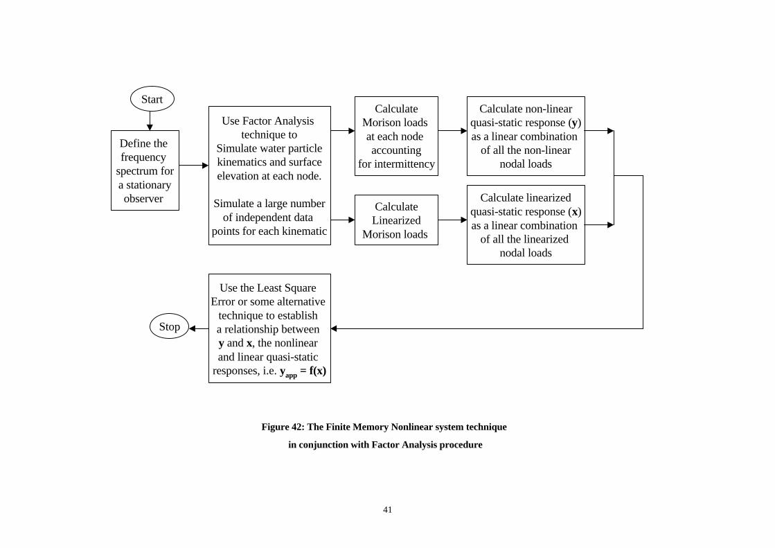
41


spectrum fora stationaryobserver

Use Factor Analysis technique to

Simulate water particlekinematics and surfaceelevation at each node.

Simulate a large numberof independent data

points for each kinematic

Use the Least Square Error or some alternative

technique to establish a relationship between y and x, the nonlinear and linear quasi-static

responses, i.e. yapp = f(x)

Stop

CalculateMorison loads at each node accounting

for intermittency

Calculate non-linearquasi-static response (y)as a linear combination

of all the non-linearnodal loads

Figure 42: The Finite Memory Nonlinear system technique

in conjunction with Factor Analysis procedure

Start

CalculateLinearized

Morison loads

Calculate linearized quasi-static response (x) as a linear combination

of all the linearized nodal loads

42

Figure 43: The level of accuracy of the nonlinear drag-only response predicted as a third order polynomial of the linearized response; no current, no intermittency

Figure 44: The level of accuracy of the nonlinear drag-only response predicted as a second order function of the linearized response; no current, no intermittency

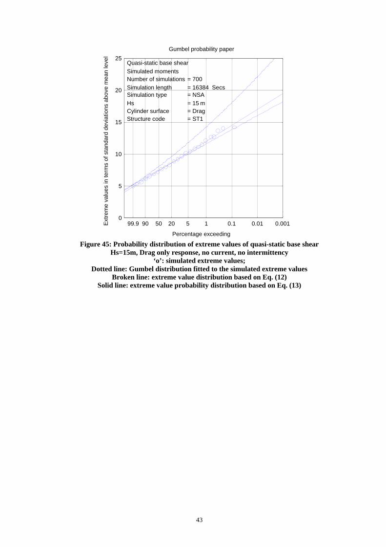
43

99.9 90 50 20 5 1 0.1 0.01 0.001 0

5

10

15

20

25


Gumbel probability paper

Ext

rem

e va

lues

in te

rms

of s

tand

ard

devi

atio

ns a

bove

mea

n le

vel

Quasi-static base shear Simulated moments Number of simulations = 700 Simulation length = 16384 Secs Simulation type = NSA Hs = 15 m Cylinder surface = Drag Structure code = ST1

Figure 45: Probability distribution of extreme values of quasi-static base shear

Hs=15m, Drag only response, no current, no intermittency ‘o’: simulated extreme values;

Dotted line: Gumbel distribution fitted to the simulated extreme values Broken line: extreme value distribution based on Eq. (12)

Solid line: extreme value probability distribution based on Eq. (13)

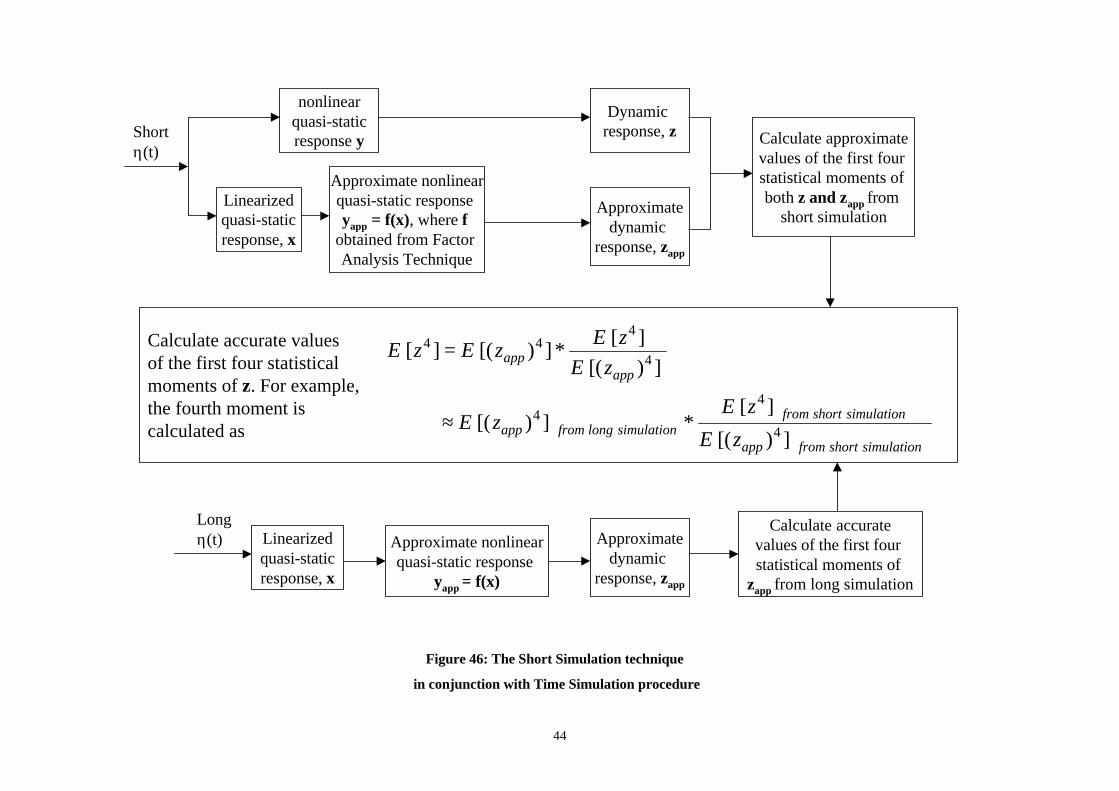
44

Figure 46: The Short Simulation technique

in conjunction with Time Simulation procedure

Shortη(t)

Linearizedquasi-staticresponse, x

Approximate nonlinearquasi-static response yapp = f(x), where f

obtained from Factor Analysis Technique

nonlinearquasi-staticresponse y

Dynamic response, z

Approximatedynamic

response, zapp

Calculate approximatevalues of the first four statistical moments of both z and zapp from

short simulation

Linearizedquasi-staticresponse, x

Approximate nonlinearquasi-static response

yapp = f(x)

Approximatedynamic

response, zapp

Longη(t)

Calculate accuratevalues of the first four statistical moments of

zapp from long simulation

Calculate accurate values of the first four statisticalmoments of z. For example,the fourth moment is calculated as

simulationshortfromapp

simulationshortfromsimulationlongfromapp

appapp

zE

zEzE

zEzE

zEzE

])([

][*])([

])([][

*])([][

4

44

4

444

≈

=

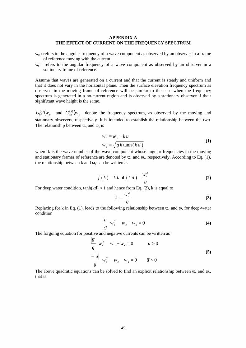
45

APPENDIX A THE EFFECT OF CURRENT ON THE FREQUENCY SPECTRUM

ωc : refers to the angular frequency of a wave component as observed by an observer in a frame

of reference moving with the current. ωs : refers to the angular frequency of a wave component as observed by an observer in a

stationary frame of reference. Assume that waves are generated on a current and that the current is steady and uniform and that it does not vary in the horizontal plane. Then the surface elevation frequency spectrum as observed in the moving frame of reference will be similar to the case when the frequency spectrum is generated in a no-current region and is observed by a stationary observer if their significant wave height is the same.

( )ccG ωηη

)( and ( )ssG ωηη)( denote the frequency spectrum, as observed by the moving and

stationary observers, respectively. It is intended to establish the relationship between the two. The relationship between ωc and ωs is

)(tanh dkkg

uk

c

sc

=

−=

ω

ωω (1)

where k is the wave number of the wave component whose angular frequencies in the moving and stationary frames of reference are denoted by ωc and ωs, respectively. According to Eq. (1), the relationship between k and ωc can be written as

g

dkkkf c2

)(tanh)(ω

== (2)

For deep water condition, tanh(kd) ≈ 1 and hence from Eq. (2), k is equal to

g

k c2ω

= (3)

Replacing for k in Eq. (1), leads to the following relationship between ωc and ωs for deep-water condition

02 =−+

sccg

uωωω (4)

The forgoing equation for positive and negative currents can be written as

00

00

2

2

<=−+

−

>=−+

ugu

ugu

scc

scc

ωωω

ωωω

(5)

The above quadratic equations can be solved to find an explicit relationship between ωc and ωs, that is

46

02

411

02

411

<−+

=

>+±−

=

u

gu

gu

u

gu

gu

s

c

s

c

ωω

ωω

m

(6)

The expression under the square root must be positive; therefore,

04

04

0041

0041

<≤

>−

≥

<≥−

>≥+

uug

uug

or

ugu

ug

u

s

s

s

s

ω

ω

ω

ω

(7)

On the other hand, ωc is always positive; therefore the first equation in (6) must have the

positive sign before the square root and also 00141 >≥−+ ugu

sω , which implies

that ωs would always be positive for the case of positive current. For negative current, ωc is always positive when the sign before the square root in (6) is positive. When the sign before the square root is negative, The following relationship must hold,

00

0141

<≥

<≤−

uor

ugu

s

s

ω

ω

(8)

According to Eq. (5), the relationship between ωs and ωc for negative current is

02 <+

−= u

gu

ccs ωωω (9)

Therefore, ωs is equal to zero when ωc = 0 or ug

c =ω . The maximum value of ωs, (ωs)max, is

obtained when the first derivative of ωs with respect to ωc is set equal to zero. As a result,

47

ug

at

ug

c

s

2ˆ

4)( max

=

=

ω

ω

(10)

Note that when current is negative, for each ωs value in the rangeug

s 40 pp ω , there are two

different ωc values, one smaller and one larger than cω̂ . The group velocity at cω̂ in the

moving frame of reference is uug

cc

g −===ω̂2

; that is, the group velocity with respect to

the current is equal to the current, but of opposite direction. Therefore the group velocity at

cω̂ for the stationary observer is equal to zero. As a result waves with frequencies greater than

cω̂ will never reach the stationary observer. In other words, only waves with frequencies in

the range ug

c 20 pp ω are of practical significance for negative currents. Consequently in the

case of negative currents, the sign before the square root in Eq. (6), must be negative. If we

choose the positive sign before the square root, then ug

c 2>ω and hence their corresponding

group velocity will be less that the absolute value of the current. That is

uug

cc

g −=<=ω2

. Therefore the acceptable relationships between ωc and ωs for both

positive and negative currents are

02

411

02

411

<−−+

=

>++−

=

u

gu

gu

u

gu

gu

s

c

s

c

ωω

ωω

(11)

The above equation can be summarised as

−+=

++−= 141

22

411

s

s

c gu

ug

gu

gu

ωω

ω (12)

For positive current ωc and ωs can be any positive numbers while for negative current they will

satisfyug

c 20 pp ω and

ug

s 40 pp ω (refer to Figures A.1 and A.2).

From Eq. (12), the first derivative of ωc with respect to ωs is

48

s

s

c

gu

gu

ωε

εω

ω

41

1

41

1

+=

=+

=′

(13)

Combining Eqs. (12) and (13), the relationship between ωc and ωs can be written as

ε

ωω

+=

12 s

c (14)

Now assume that the surface elevation frequency spectrum for the stationary observer at a given frequency ωs is ( )s

sG ωηη)( . It is intended to calculate the frequency spectrum for the observer

moving with the current at the equivalent frequency ε

ωω

+=

12 s

c . This can be achieved by

considering a small frequency interval dωs around ωs and a small frequency interval dωc around ωc, then the following relationships hold,

( ) ( )

( ) ( )

( ) ( )

( ) ( )

( )

+

==

+=+

==′

′=

′=

′=

′=

=

εω

ωε

ω

ωεε

ωω

εω

ωωωωω

ωωωωωωω

ωωωωωωω

ωωω

ωωωω

ηηηη

ηηηη

ηηηη

ηηηη

ηηηη

121

,

41;12

;1

,),14()13(.

;)(.)(

)(.)(

,

)(.)(

,

,

)()(

)()(

)()(

)()(

)()(

sc

cs

s

ss

cc

scc

scss

sscscc

sss

sscscc

ccc

scc

ccc

sss

GG

conditionswaterdeepforTherefore

gu

validareipsrelationshfollowingtheconditionswaterdeepforandEqstoAccording

depthswaterallforvalidGG

or

dGdG

Therefore

dGdG

Thereforedd

but

dGdG

(15)

Therefore,

( ) ( ) ( )

( )( ) bd

ac

dGdGdG

sc

sc

b

acc

cd

cssc

csc

d

css

s

====

=′= ∫∫∫

ωωωω

ωωωωωωωωω ηηηηηη)()()( )(.)(

(16)

49

Therefore, ( ) baG ccc ≤≤ ωωηη

)( , as observed by the moving observer, is seen as the

following frequency spectrum by the stationary observer

( ) ( ) ( )( )( )( )

( )

( )( ) bd

ac

gu

dcGG

toreducewillequationabovetheconditionswaterdeepFor

bdac

dcGG

sc

sc

s

ss

cc

ss

sc

sc

sscc

scss

====

+=

≤≤

+

==

====

≤≤′=

ωωωω

ωε

ωε

ωω

εω

ωωωω

ωωωωωω

ηηηη

ηηηη

41

121

,

*

)()(

)()(

(17)

Therefore, in deep water cases, ωc and ωs can be any positive numbers when the current is positive. In the case of negative currents, they should satisfy the following two

relationships:ug

c 20 pp ω and

ug

s 40 pp ω . The relationships between ωc and ωs for

negative and positive currents, are presented in Figures A.1 and A.2, respectively. For shallow-water condition, tanh(kd) ≈ kd and hence from Eq. (2), k is equal to

dgc

dgTL

dgk c

=

=

=ω

(18)

Replacing the above equation into Eq. (1) leads to

dgu

dgcoefd

d

dgu

coef

coef

s

c

sc

+==

+=

=

1

1

ωω

ωω

(19)

For a depth of 120m, and a current of –1.5m/s

50

equationswatershallowFromdd

coef

s

c

sc

−=

==

046.1

046.1956.0

ωω

ωω (20)

while using the deep-water equations at very low frequencies,

equationswaterdeepFrom

dd

s

c

sc

−=

=

1ωω

ωω (21)

It is therefore more appropriate to use the general equations to avoid approximations. To summarise, assuming that ( ) baG cc

c ≤≤ ωωηη)( is known, it is intended to calculate

( ) dcG sss ≤≤ ωωηη)( . According to equation (15), it is necessary to calculate both

cc and ωω ′ as functions of ωs. There are closed-form solutions for the special cases of deep-water and shallow-water conditions. But for the general case numerical techniques must be applied as follows: 1. Determine the lower and upper limits of ωc. That is, ba c ≤≤ ω . Waves with frequencies

out of this range are assumed to be insignificant. Then divide this interval into a number of equal sub-intervals and define a number of equidistant ωc values. Define ( )c

cG ωηη)( at these

cω values. 2. Calculate wave number kc for each ωc value from Eq. (2) using an appropriate numerical

technique. Also calculate sinh(kc.d) for wave components which are not in deep water, where d is the water depth. This is calculated in program wave_number2.m. These values will be applicable to the case where the current is negligible. In that case, the following steps are redundant.

3. Determine the corresponding (equivalent) ωs-eq value for each ωc value from Eq. (1). That is ukcceqs +=− ωω . Therefore, the wave number kc is associated with both ωc and their

corresponding ωs-eq values.

4. Note that the resultant ωs-eq values are not equidistant. Therefore determine the lower and upper limits of ωs-eq, that is, dc eqs ≤≤ −ω . Then divide the interval into a number of equal

sub-intervals and define a number of equidistant ωs values.

5. Calculate the wave number ks for each new ωs value by interpolation given that ωs-eq and their associated wave numbers, kc, have previously been calculated.

6. Calculate the corresponding (equivalent) ωc-eq value for each new ωs value from Eq. (1). That is uksseqc −=− ωω . Thus, ks values are associated with both equidistant ωs values

and their corresponding ωc-eq values. (The relationship between ωs and ωc for negative and positive currents are demonstrated in Figures A.3 and A.4, respectively).

7. Determine ( )eqccG −ωηη

)( by interpolation given that ωc and ( )ccG ωηη

)( are known.

51

8. Determine s

eqc

d

d

ω

ω − for each ωs value by an appropriate numerical technique. The variation

of this derivative with ωs for both negative and positive currents are demonstrated in Figures A.5 and A.6, respectively.

9. Calculate ( )ssG ωηη)( from Eq. (17). That is

( ) ( ) dcGd

dG seqc

c

s

eqcs

s ≤≤= −− ωω

ω

ωω ηηηη

)()( * . This is calculated in program

stationary_spectrum2.m. Also calculate sinh(ks.d) for those wave components which are not in deep water, where d is the water depth, in the same program. These values will replace sinh(kc.d), which were previously calculated in wave_number2.m and were only applicable to the case where the current was negligible.

10. Now that ( ) dcG sss ≤≤ ωωηη)( is known, the surface elevation at a given point can be

simulated from this spectrum, as previously described.

11. For all ωs values, their corresponding ωc-eq and ks values have already been calculated; therefore, water particle kinematics at any point can be simulated. The transfer functions for horizontal water particle velocity and acceleration at point (x2, z2), when the surface elevation is defined at point x1, are

( )( )

( )( ) ( )ϕωω

ϕ

ϕωω

∆−−−=

−=∆

∆−−=

−

−

.1exp.exp.)(

.

.

.1exp.)(sinh)(cosh

.)(

2

12

2

dzkT

iesinstabilitnumericalavoidtoconditionswaterdeepforequationfollowingtheUse

xxk

depthwatergeneraldkzk

T

seqcsu

s

s

seqcsu

(22)

and

)(.1)( sueqcsu TT ωωω −′ −=

(23)

It should be noted that for negative current, ε at ( )ugs 4=ω in Eq. (17) is zero, and hence

( )ssG ωηη)( would be infinity. It is therefore better to keep ( ) ( )ugs 498.00 pp ω . Therefore,

( ) ( )ugc 43.00 pp ω or ( ) ( )ugf c 068.00 pp . For a –1m/s current,

Hzfc 667.00 pp . This means that wave components with periods greater than 1.5 seconds will be included. Waves with shorter periods are not particularly significant. For current of –1.5 m/s, waves with periods longer than 2.25 seconds are included.

52

0 2 4 6 8 10 -3

-2

-1

0

1

2

3

wc: angular frequency (rad/sec) for the observer moving with the current

Relationship between ws and wc for a current of -g/8 = -1.2257 m/sec

ws

: ang

ular

freq

uenc

y (r

ad/s

ec)

for

the

stat

iona

ry o

bser

ver

(ws)max = g/(4|u|)

(wc = g/|u|; ws = 0

wc = g/(2|u|)

Figure A.1: Effect of negative current on wave frequency (deep-water condition assumed)

0 2 4 6 8 10 0

5

10

15

20

25


Relationship between ws and wc for a current of g/8 = 1.2257 m/sec

ws

: ang

ular

freq

uenc

y (r

ad/s

ec)

for

the

stat

iona

ry o

bser

ver

Figure A.2: Effect of positive current on wave frequency (deep-water condition assumed)

53

0 0.5 1 1.5 2 2.5 3 0

0.2

0.4

0.6

0.8

1

1.2

1.4

1.6

1.8

2


Relationship between ws and wc for a current of g/8 = -1.2257

m/sec

ws

: ang

ular

freq

uenc

y (r

ad/s

ec)

for

the

stat

iona

ry

obse

rver

Figure A.3: Effect of negative current on wave frequency (general water depth condition assumed)

0 0.5 1 1.5 2 2.5 3 0

0.5

1

1.5

2

2.5

3

3.5

4

4.5


Relationship between ws and wc for a current of g/8 = 1.2257 m/sec

ws

: ang

ular

freq

uenc

y (r

ad/s

ec)

for

the

stat

iona

ry o

bser

ver

Figure A.4: Effect of positive current on wave frequency (general water depth condition assumed)

54

0 0.5 1 1.5 2 1

1.5

2

2.5

3

3.5

4

ws : angular frequency (rad/sec) for the stationary observer

Relationship between derivative of wc and ws for u = -1.2257 m/sec

Der

ivat

ive

of w

c w

ith r

espe

ct to

ws

Figure A.5: Derivative of ωc with respect to ωs for negative current (general water depth condition assumed)

0 1 2 3 4 5 0.55

0.6

0.65

0.7

0.75

0.8

0.85

0.9

0.95

1

ws : angular frequency (rad/sec) for the stationary observer

Relationship between derivative of wc and ws for u = 1.2257 m/sec

Der

ivat

ive

of w

c w

ith r

espe

ct to

ws

Figure A.6: Derivative of ωc with respect to ωs for positive current (general water depth condition assumed)

55

APPENDIX B LOAD INTERMITTENCY IN THE SPLASH ZONE

The elevation of the nodal point A above seabed is denoted by z and the surface elevation above the mean water level at that point is denoted by η(t). Then when water depth + η(t) is greater than z, the member is submerged and subject to loading; otherwise the member is exposed and receives no loading. This situation can be represented by the Heavyside function which is equal to one when its argument is positive and zero when its argument is negative.

00)(01)(

≤=>=

xxHxxH

(1)

The Heavyside function can be defined as

01)(00)(01)(

2)(1

)(

<−===>=

+=

xxsignxxsignxxsign

xsignxH

(2)

Therefore, the loading for points which are subject to intermittency, must be multiplied by )])([( ztdepthwaterH −+η (3) Points which are above or below the mean water level by up to six times the standard deviation of the surface elevation (i.e. 1.5*Hs) can be considered subject to intermittency. For other points below the mean water level, (η(t) – z) is always positive and hence the Heavyside function will always be equal to unity. There is, therefore, no need to multiply the loads by this function.

56

APPENDIX C CROSS-COVARIANCE MATRIX OF WATER PARTICLE KINEMATICS

Short-crested (directional) seas can be modelled as the sum of a large number of progressive linear waves of different amplitudes travelling in different directions with random phases (Borgman, 1969). Let x and y be the coordinates in an arbitrary horizontal Cartesian coordinate system such that the positive y axis is 90 degrees anti-clockwise from the positive x axis. The z axis is vertically upwards. The waves are assumed to travel in a direction θ measured anti-clockwise from the positive x axis. The cross-covariances between nodal kinematics at nodes I and J are given in the following tables (Borgman, 1977) where f stands for wave frequency and ω = 2πf is its angular frequency. Gηη(f) and D(f,θ) are the surface elevation frequency spectrum and the spreading function, respectively. Γhv and Γw stand for transfer functions converting the surface elevation to horizontal and vertical water particle kinematics, respectively and ]sincos[ θθϕ yxk ∆+∆=∆ is the phase shift between kinematics, where k is the wave number for the wave component with frequency f, and .∆x = xJ – xI and .∆y = yJ – yI. In the following equations η refers to surface elevation, U, V and W to x, y and z components of water particle velocity, and UD, VD and WD refer to x, y and z components of water particle acceleration. Table 1: Cross-covariances between the X component of water particle velocity at

node I and kinematics at node J E[(U)I . (U)J] = ( ) θϕθθ

θ

θηη ddfzzfDfG jhvihv

f

f∫ ∫

∆ΓΓ

max

min

max

min

cos)()(),()()(cos2

E[[(U)I . (UD)J] = ( ) θϕωθθ

θ


f

f∫ ∫

∆ΓΓ

max

min

max

min

sin)()(),()()(cos2

E[[(U)I . (V)J] = ( ) θϕθθθ

θ


f

f∫ ∫

∆ΓΓ

max

min

max

min

cos)()(),()()cos()sin(

E[[(U)I . (VD)J] = ( ) θϕωθθθ

θ


f

f∫ ∫

∆ΓΓ

max

min

max

min

sin)()(),()()cos()sin(

E[[(U)I . (W)J] = ( ) θϕθθ

θ

θηη ddfzzfDfG jwihv

f

f∫ ∫

∆ΓΓ

max

min

max

min

sin)()(),()()cos(

E[[(U)I . (WD)J] = ( ) θϕωθθ

θ


f

f∫ ∫

∆ΓΓ−

max

min

max

min

cos)()(),()()cos(

E[[(U)I . (η)J] = ( ) θϕθθ

θ

θηη ddfzfDfG ihv

f

f∫ ∫

∆Γ

max

min

max

min

cos)(),()()cos(

57

Table 2: Cross-covariances between the X component of water particle acceleration at node I and kinematics at node J

E[(UD)I . (U)J] = ( ) θϕωθθ

θ


f

f∫ ∫

∆ΓΓ−

max

min

max

min

sin)()(),()()(cos2

E[[(UD)I . (UD)J] = ( ) θϕωθθ

θ


f

f∫ ∫

∆ΓΓ

max

min

max

min

cos)()(),()()(cos 22

E[[(UD)I . (V)J] = ( ) θϕωθθθ

θ


f

f∫ ∫

∆ΓΓ−

max

min

max

min


E[[(UD)I . (VD)J] = ( ) θϕωθθθ

θ


f

f∫ ∫

∆ΓΓ

max

min

max

min

cos)()(),()()cos()sin( 2

E[[(UD)I . (W)J] = ( ) θϕωθθ

θ


f

f∫ ∫

∆ΓΓ

max

min

max

min

cos)()(),()()cos(

E[[(UD)I . (WD)J] = ( ) θϕωθθ

θ


f

f∫ ∫

∆ΓΓ

max

min

max

min

sin)()(),()()cos( 2

E[[(UD)I . (η)J] = ( ) θϕωθθ

θ

θηη ddfzfDfG ihv

f

f∫ ∫

∆Γ−

max

min

max

min

sin)(),()()cos(

Table 3: Cross-covariances between the Y component of water particle velocity at node I

and kinematics at node J E[(V)I . (U)J] = ( ) θϕθθθ

θ


f

f∫ ∫

∆ΓΓ

max

min

max

min

cos)()(),()()cos()sin(

E[[(V)I . (UD)J] = ( ) θϕωθθθ

θ


f

f∫ ∫

∆ΓΓ

max

min

max

min


E[[(V)I . (V)J] = ( ) θϕθθ

θ


f

f∫ ∫

∆ΓΓ

max

min

max

min

cos)()(),()()(sin2

E[[(V)I . (VD)J] = ( ) θϕωθθ

θ


f

f∫ ∫

∆ΓΓ

max

min

max

min

sin)()(),()()(sin2

E[[(V)I . (W)J] = ( ) θϕθθ

θ


f

f∫ ∫

∆ΓΓ

max

min

max

min

sin)()(),()()sin(

E[[(V)I . (WD)J] = ( ) θϕωθθ

θ


f

f∫ ∫

∆ΓΓ−

max

min

max

min

cos)()(),()()sin(

E[[(V)I . (η)J] = ( ) θϕθθ

θ

θηη ddfzfDfG ihv

f

f∫ ∫

∆Γ

max

min

max

min

cos)(),()()sin(

58

Table 4: Cross-covariances between the Y component of water particle acceleration at node I and kinematics at node J

E[(VD)I . (U)J] ( ) θϕωθθθ

θ


f

f∫ ∫

∆ΓΓ−

max

min

max

min


E[[(VD)I . (UD)J] = ( ) θϕωθθθ

θ


f

f∫ ∫

∆ΓΓ

max

min

max

min

cos)()(),()()cos()sin( 2

E[[(VD)I . (V)J] = ( ) θϕωθθ

θ


f

f∫ ∫

∆ΓΓ−

max

min

max

min

sin)()(),()()(sin2

E[[(VD)I . (VD)J] = ( ) θϕωθθ

θ


f

f∫ ∫

∆ΓΓ

max

min

max

min

cos)()(),()()(sin 22

E[[(VD)I . (W)J] = ( ) θϕωθθ

θ


f

f∫ ∫

∆ΓΓ

max

min

max

min

cos)()(),()()sin(

E[[(VD)I . (WD)J] = ( ) θϕωθθ

θ


f

f∫ ∫

∆ΓΓ

max

min

max

min

sin)()(),()()sin( 2

E[[(VD)I . (η)J] = ( ) θϕωθθ

θ

θηη ddfzfDfG ihv

f

f∫ ∫

∆Γ−

max

min

max

min

sin)(),()()sin(

Table 5: Cross-covariances between the vertical component of water particle velocity at node I and kinematics at node J

E[(W)I . (U)J] = ( ) θϕθθ

θ

θηη ddfzzfDfG jhviw

f

f∫ ∫

∆ΓΓ−

max

min

max

min

sin)()(),()()cos(

E[[(W)I . (UD)J] = ( ) θϕωθθ

θ


f

f∫ ∫

∆ΓΓ

max

min

max

min

cos)()(),()()cos(

E[[(W)I . (V)J] = ( ) θϕθθ

θ


f

f∫ ∫

∆ΓΓ−

max

min

max

min

sin)()(),()()sin(

E[[(W)I . (VD)J] = ( ) θϕωθθ

θ


f

f∫ ∫

∆ΓΓ

max

min

max

min

cos)()(),()()sin(

E[[(W)I . (W)J] = ( ) θϕθ

θ

θηη ddfzzfDfG jwiw

f

f∫ ∫

∆ΓΓ

max

min

max

min

cos)()(),()(

E[[(W)I . (WD)J] = ( ) θϕωθ

θ


f

f∫ ∫

∆ΓΓ

max

min

max

min

sin)()(),()(

E[[(W)I . (η)J] = ( ) θϕθ

θ

θηη ddfzfDfG iw

f

f∫ ∫

∆Γ−

max

min

max

min

sin)(),()(

59

Table 6: Cross-covariances between the vertical component of water particle acceleration at node I and kinematics at node J

E[(WD)I . (U)J] = ( ) θϕωθθ

θ


f

f∫ ∫

∆ΓΓ−

max

min

max

min

cos)()(),()()cos(

E[[(WD)I . (UD)J] = ( ) θϕωθθ

θ


f

f∫ ∫

∆ΓΓ−

max

min

max

min

sin)()(),()()cos( 2

E[[(WD)I . (V)J] = ( ) θϕωθθ

θ


f

f∫ ∫

∆ΓΓ−

max

min

max

min

cos)()(),()()sin(

E[[(WD)I . (VD)J] = ( ) θϕωθθ

θ


f

f∫ ∫

∆ΓΓ−

max

min

max

min

sin)()(),()()sin( 2

E[[(WD)I . (W)J] = ( ) θϕωθ

θ


f

f∫ ∫

∆ΓΓ−

max

min

max

min

sin)()(),()(

E[[(WD)I . (WD)J] = ( ) θϕωθ

θ


f

f∫ ∫

∆ΓΓ

max

min

max

min

cos)()(),()( 2

E[[(WD)I . (η)J] = ( ) θϕωθ

θ

θηη ddfzfDfG iw

f

f∫ ∫

∆Γ−

max

min

max

min

cos)(),()(

Table 7: Cross-covariances between surface elevation at node I and kinematics at node J

E[(η)I . (U)J] = ( ) θϕθθ

θ

θηη ddfzfDfG jhv

f

f∫ ∫

∆Γ

max

min

max

min

cos)(),()()cos(

E[[(η)I . (UD)J] = ( ) θϕωθθ

θ

θηη ddfzfDfG jhv

f

f∫ ∫

∆Γ

max

min

max

min

sin)(),()()cos(

E[[(η)I . (V)J] = ( ) θϕθθ

θ

θηη ddfzfDfG jhv

f

f∫ ∫

∆Γ

max

min

max

min

cos)(),()()sin(

E[[(η)I . (VD)J] = ( ) θϕωθθ

θ

θηη ddfzfDfG jhv

f

f∫ ∫

∆Γ

max

min

max

min

sin)(),()()sin(

E[[(η)I . (W)J] = ( ) θϕθ

θ

θηη ddfzfDfG jw

f

f∫ ∫

∆Γ

max

min

max

min

sin)(),()(

E[[(η)I . (WD)J] = ( ) θϕωθ

θ

θηη ddfzfDfG jw

f

f∫ ∫

∆Γ−

max

min

max

min

cos)(),()(

E[[(η)I . (η)J] = ( ) θϕθ

θ

θηη ddffDfG

f

f∫ ∫

∆

max

min

max

min

cos),()(

Printed and published by the Health and Safety ExecutiveC30 1/98

60

Printed and published by the Health and Safety ExecutiveC30 1/98

61

Printed and published by the Health and Safety ExecutiveC0.35 4/02

OTO 2002/011

£25.00 9 780717 623426

ISBN 0-7176-2342-4

Documents

Efficient techniques for risk assessment of space frame