Embed Size (px)
Citation preview

International Journal of Scientific and Research Publications, Volume 2, Issue 9, September 2012 1
ISSN 2250-3153
www.ijsrp.org
EIENSTEIN FIELD EQUATIONS AND
HEISENBERG’S PRINCIPLE OF
UNCERTAINLY THE CONSUMMATION
OF GTR AND UNCERTAINTY
PRINCIPLE
1DR K N PRASANNA KUMAR,
2PROF B S KIRANAGI AND
3PROF C S BAGEWADI
ABSTRACT: The Einstein field equations (EFE) or Einstein's equations are a set of
10 equations in Albert Einstein's general theory of relativity which describe the fundamental
interaction (e&eb) of gravitation as a result of space time being curved by matter and energy. First published by Einstein in 1915 as a tensor
equation, the EFE equate spacetime curvature (expressed by the Einstein tensor) with (=) the energy and momentum tensor within that spacetime (expressed by the stress–energy
tensor).Both space time curvature tensor and energy and momentum tensor is classified in to
various groups based on which objects they are attributed to. It is to be noted that the total amount of energy and mass in the Universe is zero. But as is said in different context, it is like
the Bank Credits and Debits, with the individual debits and Credits being conserved, holistically, the conservation and preservation of Debits and Credits occur, and manifest in the form of
General Ledger. Transformations of energy also take place individually in the same form and if all such transformations are classified and written as a Transfer Scroll, it should tally with the total,
universalistic transformation. This is a very important factor to be borne in mind. Like accounts
are classifiable based on rate of interest, balance standing or the age, we can classify the factors and parameters in the Universe, be it age, interaction ability, mass, energy content. Even virtual
particles could be classified based on the effects it produces. These aspects are of paramount importance in the study. When we write A+b+5, it means that we are adding A to B or B to A
until we reach 5. Similarly, if we write A-B=0, it means we are taking away B from A and there
may be time lag until we reach zero. There may also be cases in which instantaneous results are reached, which however do not affect the classification. By means of such a classification we
obtain the values of Einstein Tensor and Momentum Energy Tensor, which are in fact the solutions to the Einstein‘s Field Equation. Terms ―e‖ and ―eb‖ are used for better comprehension
of the lay reader. It has no other attribution or ascription whatsoever in the context of the paper.
For the sake of simplicity, we shall take the equality case of Heisenberg’s Principle Of Uncertainty for easy consolidation and consubstantiation process. The “greater than”
case can be attended to in a similar manner, with the symbolof”greater than” incorporated in the paper series.
INTRODUCTION:
Similar to the way that electromagnetic fields are determined (eb)
using charges and currents via Maxwell's equations, the EFE are used to determine the spacetime geometry resulting from the presence of mass-energy and linear momentum, that
is, they (eb) determine the metric of spacetime for a given arrangement of stress–energy in the spacetime. The relationship between the metric tensor and the Einstein tensor allows the EFE to
be written as a set of non-linear partial differential equations when used in this way. The
solutions of the EFE are the components of the metric tensor. The inertial trajectories of particles and radiation (geodesics) in the resulting geometry are then calculated using the geodesic
equation. As well as obeying local energy-momentum conservation, the EFE reduce to Newton's

International Journal of Scientific and Research Publications, Volume 2, Issue 9, September 2012 2
ISSN 2250-3153
www.ijsrp.org
law of gravitation where the gravitational field is weak and velocities are much less than
the speed of light. Solution techniques for the EFE include simplifying assumptions such as symmetry. Special classes of exact solutions are most often studied as they model many
gravitational phenomena, such as rotating black holes and the expanding universe. Further simplification is achieved in approximating the actual spacetime as flat spacetime with a small
deviation, leading to the linearised EFE. These equations are used to study phenomena such
as gravitational waves.
Mathematical form
The Einstein field equations (EFE) may be written in the form:
where is the Ricci curvature tensor, the scalar curvature, the metric tensor, is
the cosmological constant, is Newton's gravitational constant, the speed of light,in vacuum,
and the stress–energy tensor.
The EFE is a tensor equation relating a set of symmetric 4 x 4 tensors. Each tensor has 10
independent components. The four Bianchi identities reduce the number of independent equations from 10 to 6, leaving the metric with four gauge fixing degrees of freedom, which
correspond to the freedom to choose a coordinate system.
Although the Einstein field equations were initially formulated in the context of a four-
dimensional theory, some theorists have explored their consequences in n dimensions. The equations in contexts outside of general relativity are still referred to as the Einstein field
equations. The vacuum field equations (obtained when T is identically zero) define Einstein manifolds. Despite the simple appearance of the equations they are, in fact, quite complicated.
Given a specified distribution of(e&eb) matter and energy in the form of a stress–energy tensor,
the EFE are understood to be equations for the metric tensor , as both the Ricci tensor and
scalar curvature depend on the metric in a complicated nonlinear manner. In fact, when fully written out, the EFE are a system of 10 coupled, nonlinear, hyperbolic-elliptic partial differential
equations.
One can write the EFE in a more compact form by defining the Einstein tensor
Which is a symmetric second-rank tensor that is a function of the metric? The EFE can then be written as
Using geometrized units where G = c = 1, this can be rewritten as
The expression on the left represents the curvature of spacetime as (eb) determined by the metric; the expression on the right represents the matter/energy content of spacetime. The EFE
can then be interpreted as a set of equations dictating how matter/energy determines (eb) the curvature of spacetime.Or, curvature of space and time dictates the diffusion of matter energy.
These equations, together with the geodesic equation, which dictates how freely-falling moves through space-time matter, form the core of the mathematical formulation of general relativity.

International Journal of Scientific and Research Publications, Volume 2, Issue 9, September 2012 3
ISSN 2250-3153
www.ijsrp.org
Sign convention
The above form of the EFE is the standard established by Misner, Thorne, and Wheeler. The
authors analyzed all conventions that exist and classified according to the following three signs (S1, S2, and S3):
The third sign above is related to the choice of convention for the Ricci tensor:
With these definitions Misner, Thorne, and Wheeler classify themselves as , whereas
Weinberg (1972) is , Peebles (1980) and Efstathiou (1990) are while
Peacock (1994), Rindler (1977), Atwater (1974), Collins Martin & Squires (1989) are .
Authors including Einstein have used a different sign in their definition for the Ricci tensor which
results in the sign of the constant on the right side being negative
The sign of the (very small) cosmological term would change in both these versions, if the +−−− metric sign convention is used rather than the MTW −+++ metric sign convention adopted here.
Equivalent formulations
Taking the trace of both sides of the EFE one gets
Which simplifies to
If one adds times this to the EFE, one gets the following equivalent "trace-reversed"
form
Reversing the trace again would restore the original EFE. The trace-reversed form may be more convenient in some cases (for example, when one is interested in weak-field limit and can
replace in the expression on the right with the Minkowski metric without significant loss of accuracy).

International Journal of Scientific and Research Publications, Volume 2, Issue 9, September 2012 4
ISSN 2250-3153
www.ijsrp.org
The cosmological constant
Einstein modified his original field equations to include a cosmological term proportional to
the metric It is to be noted that even constants like gravitational field, cosmological constant, depend upon the objects for which they are taken in to consideration and total of these can be
classified based on the parameterization of objects.
The constant is the cosmological constant. Since is constant, the energy conservation law is unaffected.
The cosmological constant term was originally introduced by Einstein to allow for a static universe (i.e., one that is not expanding or contracting). This effort was unsuccessful for two
reasons: the static universe described by this theory was unstable, and observations of distant
galaxies by Hubble a decade later confirmed that our universe is, in fact, not static
but expanding. So was abandoned, with Einstein calling it the "biggest blunder [he] ever
made". For many years the cosmological constant was almost universally considered to be 0.Despite Einstein's misguided motivation for introducing the cosmological constant term, there is
nothing inconsistent with the presence of such a term in the equations. Indeed, recent
improved astronomical techniques have found that a positive value of is needed to explain
the accelerating universe Einstein thought of the cosmological constant as an independent
parameter, but its term in the field equation can also be moved algebraically to the other side, written as part of the stress–energy tensor:
The resulting vacuum energy is constant and given by
The existence of a cosmological constant is thus equivalent to the existence of a non-zero
vacuum energy. The terms are now used interchangeably in general relativity.
Conservation of energy and momentum
General relativity is consistent with the local conservation of energy and momentum expressed as
.
Derivation of local energy-momentum conservation
Which expresses the local conservation of stress–energy This conservation law is a physical
requirement? With his field equations Einstein ensured that general relativity is consistent with this conservation condition.
Nonlinearity
The nonlinearity of the EFE distinguishes general relativity from many other fundamental physical
theories. For example, Maxwell's equations of electromagnetism are linear in theelectric and magnetic fields, and charge and current distributions (i.e. the sum of two
solutions is also a solution); another example is Schrödinger's equation of quantum mechanics
which is linear in the wavefunction.

International Journal of Scientific and Research Publications, Volume 2, Issue 9, September 2012 5
ISSN 2250-3153
www.ijsrp.org
The correspondence principle
The EFE reduce to Newton's law of gravity by using both the weak-field approximation and
the slow-motion approximation. In fact, the constant G appearing in the EFE is determined by making these two approximations.
Vacuum field equation
If the energy-momentum tensor is zero in the region under consideration, then the field
equations are also referred to as the vacuum field equations. By setting in the trace -reversed field equations, the vacuum equations can be written as
In the case of nonzero cosmological constant, the equations are
The solutions to the vacuum field equations are called vacuum solutions. Flat Minkowski space is the simplest example of a vacuum solution. Nontrivial examples include the Schwarzschild
solution and the Kerr solution.
Manifolds with a vanishing Ricci tensor, , are referred to as Ricci-flat manifolds and
manifolds with a Ricci tensor proportional to the metric as Einstein manifolds.
Einstein–Maxwell equations
If the energy-momentum tensor is that of an electromagnetic field in free space, i.e. if
the electromagnetic stress–energy tensor
is used, then the Einstein field equations are called the Einstein–Maxwell
equations (with cosmological constant Λ, taken to be zero in conventional relativity theory):
Additionally, the covariant Maxwell Equations are also applicable in free space:
Where the semicolon represents a covariant derivative, and the brackets denote anti-
summarization. The first equation asserts that the 4-divergence of the two-form F is zero, and the second that its exterior derivative is zero. From the latter, it follows by the Poincaré
lemma that in a coordinate chart it is possible to introduce an electromagnetic field
potential such that
In which the comma denotes a partial derivative. This is often taken as equivalent to the covariant Maxwell equation from which it is derived however, there are global solutions of the
International Journal of Scientific and Research Publications, Volume 2, Issue 9, September 2012 6
ISSN 2250-3153
www.ijsrp.org
equation which may lack a globally defined potential.[9]
Solutions
The solutions of the Einstein field equations are metrics of spacetime. The solutions are hence often called 'metrics'. These metrics describe the structure of the spacetime including the inertial
motion of objects in the spacetime. As the field equations are non-linear, they cannot always be
completely solved (i.e. without making approximations). For example, there is no known complete solution for a spacetime with two massive bodies in it (which is a theoretical model of a
binary star system, for example). However, approximations are usually made in these cases. These are commonly referred to as post-Newtonian approximations. Even so, there are
numerous cases where the field equations have been solved completely, and those are
called exact solutions. The study of exact solutions of Einstein's field equations is one of the activities of cosmology. It leads to the prediction of black holes and to different models of
evolution of the universe.
The linearised EFE
The nonlinearity of the EFE makes finding exact solutions difficult. One way of solving the field equations is to make an approximation, namely, that far from the source(s) of gravitating matter,
the gravitational field is very weak and the spacetime approximates that of Minkowski space. The metric is then written as the sum of the Minkowski metric and a term representing the deviation
of the true metric from the Minkowski metric. This linearization procedure can be used to discuss the phenomena of gravitational radiation.
Ricci curvature
In differential geometry, the Ricci curvature tensor, named after Gregorio Ricci-Curbastro,
represents the amount by which the volume element of a geodesic ball in a curved Riemannian deviates from that of the standard ball in Euclidean space. As such, it provides one
way of measuring the degree to which the geometry determined by a given Riemannian
metric might differ from that of ordinary Euclidean n-space. The Ricci tensor is defined on any pseudo-Riemannian manifold, as a trace of the Riemann curvature tensor. Like the metric
itself, the Ricci tensor is a symmetric bilinear form on the tangent space of the manifold (Besse 1987, p. 43).
In relativity theory, the Ricci tensor is the part of the curvature of space-time that determines the
degree to which matter will tend to converge or diverge in time (via the Raychaudhuri equation). It is related to the matter content of the universe by means of the Einstein field equation. In
differential geometry, lower bounds on the Ricci tensor on a Riemannian manifold allow one to
extract global geometric and topological information by comparison (cf. comparison theorem) with the geometry of a constant curvature space form. If the Ricci tensor satisfies the vacuum
Einstein equation, then the manifold is an Einstein manifold, which has been extensively studied (cf. Besse 1987). In this connection, the flow equation governs the evolution of a given metric to
an Einstein metric, the precise manner in which this occurs ultimately leads to the solution of the
Poincaré conjecture.
Scalar curvature
In Riemannian geometry, the scalar curvature (or Ricci scalar) is the simplest curvature invariant
of a Riemannian manifold. To each point on a Riemannian manifold, it assigns a single real
number determined by the intrinsic geometry of the manifold near that point. Specifically, the scalar curvature represents the amount by which the volume of a geodesic ball in a curved
Riemannian manifold deviates from that of the standard ball in Euclidean space. In two dimensions, the scalar curvature is twice the Gaussian curvature, and completely characterizes
the curvature of a surface. In more than two dimensions, however, the curvature of Riemannian
manifolds involves more than one functionally independent quantity.
In general relativity, the scalar curvature is the Lagrangian density for the Einstein–Hilbert action.
International Journal of Scientific and Research Publications, Volume 2, Issue 9, September 2012 7
ISSN 2250-3153
www.ijsrp.org
The Euler–Lagrange equations for this Lagrangian under variations in the metric constitute the
vacuum Einstein field equations, and the stationary metrics are known as Einstein metrics. The scalar curvature is defined as the trace of the Ricci tensor, and it can be characterized as a
multiple of the average of the sectional curvatures at a point. Unlike the Ricci tensor and sectional curvature, however, global results involving only the scalar curvature are extremely
subtle and difficult. One of the few is the positive mass theorem of Richard Schoen, Shing-Tung
Yau and Edward Witten. Another is the Yamabe problem, which seeks extremal metrics in a given conformal class for which the scalar curvature is constant.
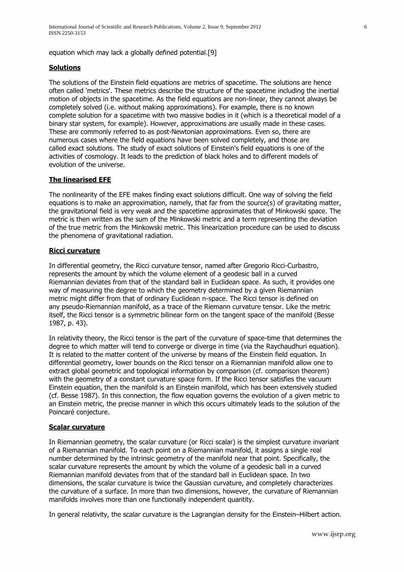
Metric tensor (general relativity)
.
Metric tensor of spacetime in general relativity written as a matrix.
In general relativity, the metric tensor (or simply, the metric) is the fundamental object of study.
It may loosely be thought of as a generalization of the gravitational field familiar from Newtonian gravitation. The metric captures all the geometric and causal structure inspacetime, being used
to define notions such as distance, volume, curvature, angle, future and past.
Notation and conventions: Throughout this article we work with a metric signature that is mostly positive (− + + +); see sign convention. As is customary in relativity, units are used where
the speed of light c = 1. The gravitation constant G will be kept explicit. The summation, where repeated indices are automatically summed over, is employed.
COSMOLOGICAL CONSTANT:
In physical cosmology, the cosmological constant (usually denoted by the Greek capital
letter lambda: Λ) was proposed by Albert Einstein as a modification of his original theory of general relativity to achieve a stationary universe. Einstein abandoned the concept after the
observation of the Hubble redshift indicated that the universe might not be stationary, as he had
based his theory on the idea that the universe is unchanging. However, the discovery of cosmic acceleration in 1998 has renewed interest in a cosmological constant.
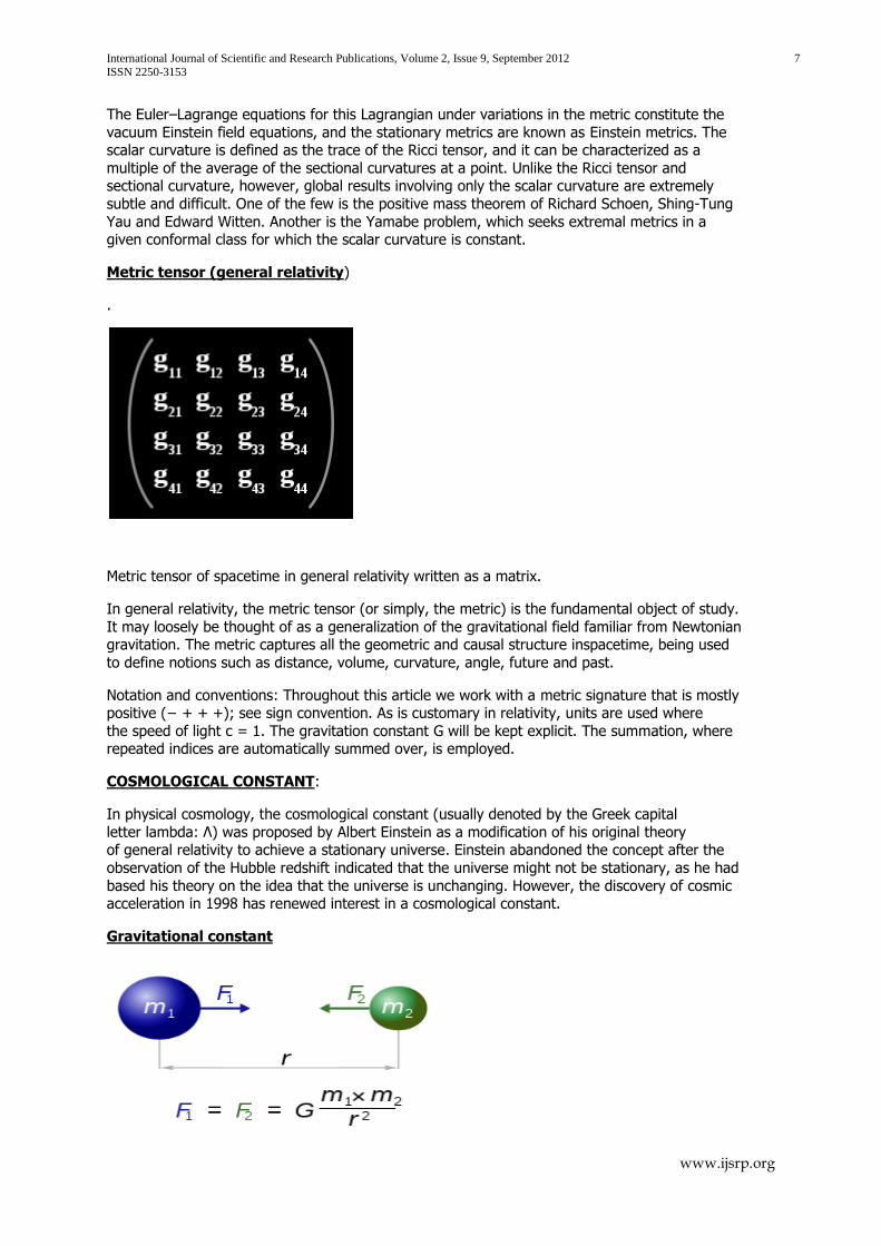
Gravitational constant

International Journal of Scientific and Research Publications, Volume 2, Issue 9, September 2012 8
ISSN 2250-3153
www.ijsrp.org
The gravitational constant denoted by letter G, is an empirical physical constant involved in the
calculation(s) of gravitational force between two bodies.G should not be confused with "little g" (g), which is the local gravitational field (equivalent to the free-fall acceleration, especially that at
the Earth's surface..
Speed of light.
The speed of light in vacuum, usually denoted by c, is a universal physical constant important in many areas of physics. Its value is 299,792,458 metres per second, a figure that is exact since
the length of the metre is defined from this constant and the international standard for time. In imperial units this speed is approximately 186,282 miles per second. According to special
relativity, c is the maximum speed at which all energy, matter, and information in
the universe can travel. It is the speed at which all massless particles and associated fields (including electromagnetic radiation such aslight) travel in vacuum. It is also
the speed of gravity (i.e. of gravitational waves) predicted by current theories. Such particles and waves travel at c regardless of the motion of the source or the inertial frame of reference of the
observer. In the Theory, c interrelates space and time, and also appears in the famous equation of mass–energy equivalence = mc2
The speed at which light propagates through transparent materials, such as glass or air, is less
than c. The ratio between cand the speed v at which light travels in a material is called
the refractive index n of the material (n = c / v). For example, for visible light the refractive index of glass is typically around 1.5, meaning that light in glass travels atc / 1.5
≈ 200,000 km/s; the refractive index of air for visible light is about 1.0003, so the speed of light in air is about90 km/s slower than c.
In most practical cases, light can be thought of as moving "instantaneously", but for long
distances and very sensitive measurements the finite speed of light has noticeable effects. In communicating with distant space probes, it can take minutes to hours for a message to get from
Earth to the spacecraft or vice versa. The light we see from stars left them many years ago,
allowing us to study the history of the universe by looking at distant objects. The finite speed of light also limits the theoretical maximum speed of computers, since information must be sent
within the computer from chip to chip. Finally, the speed of light can be used with time of flight measurements to measure large distances to high precision.
Ole Rømer first demonstrated in 1676 that light travelled at a finite speed (as opposed to
instantaneously) by studying the apparent motion of Jupiter's moon Io. In 1865, James Clerk Maxwell proposed that light was an electromagnetic wave, and therefore travelled at the
speed c appearing in his theory of electromagnetism In 1905, Albert Einstein postulated that the
speed of light with respect to any inertial frame is independent of the motion of the light source and explored the consequences of that postulate by deriving the special theory of
relativity and showing that the parameter c had relevance outside of the context of light and electromagnetism. After centuries of increasingly precise measurements, in 1975 the speed of
light was known to be 299,792,458 m/s with a measurement uncertainty of 4 parts per billion. In
1983, the metrewas redefined in the International System of Units (SI) as the distance travelled by light in vacuum in 1⁄299,792,458 of asecond. As a result, the numerical value of c in metres
per second is now fixed exactly by the definition of the metre
] Numerical value, notation, and units
The speed of light in vacuum is usually denoted by c, for "constant" or the Latin celeritas (meaning "swiftness"). Originally, the symbol V was used, introduced by James
Clerk Maxwell in 1865. In 1856, Wilhelm Eduard Weber and Rudolf Kohlrausch used c for a constant later shown to equal √2 times the speed of light in vacuum. In 1894, Paul
Druderedefined c with its modern meaning. Einstein used V in his original German-language papers on special relativity in 1905, but in 1907 he switched to c, which by then had become the
standard symbol.
Sometimes c is used for the speed of waves in any material medium, and c0 for the speed of

International Journal of Scientific and Research Publications, Volume 2, Issue 9, September 2012 9
ISSN 2250-3153
www.ijsrp.org
light in vacuum This subscripted notation, which is endorsed in official SI literature, has the same
form as other related constants: namely, μ0for the vacuum permeability or magnetic constant, ε0 for the vacuum permittivity or electric constant, and Z0 for the impedance. This
article uses c exclusively for the speed of light in vacuum.
In the International System of Units (SI), the metre is defined as the distance light travels in vacuum in 1⁄299,792,458 of a second. This definition fixes the speed of light in vacuum at
exactly 299,792,458 m/s. As a dimensional physical constant, the numerical value of c is different for different unit systems. In branches of physics in which cappears often, such as in relativity, it
is common to use systems of natural units of measurement in which c = 1 Using these
units, c does not appear explicitly because multiplication or division by 1 does not affect the result.
Fundamental role in physics
Speed at which light waves propagate in vacuum is independent both of the motion of the wave
source and of the inertial frame of reference of the observer This invariance of the speed of light was postulated by Einstein in 1905 after being motivated by Maxwell's theory of
electromagnetism and the lack of evidence for the luminiferous aether; it has since been consistently confirmed by many experiments. It is only possible to verify experimentally that the
two-way speed of light (for example, from a source to a mirror and back again) is frame-
independent, because it is impossible to measure the one-way speed of light (for example, from a source to a distant detector) without some convention as to how clocks at the source and at
the detector should be synchronized. However, by adopting Einstein synchronization for the clocks, the one-way speed of light becomes equal to the two-way speed of light by
definition. The special theory of relativity explores the consequences of this invariance of c with the assumption that the laws of physics are the same in all inertial frames of reference. One
consequence is that c is the speed at which all massless particles and waves, including light,
must travel in vacuum.
The Lorentz factor γ as a function of velocity. It starts at 1 and approaches infinity as v approaches c.
Special relativity has many counterintuitive and experimentally verified implications These include
the equivalence of mass and energy (E = mc2), length contraction (moving objects shorten),[ and time dilation (moving clocks run slower). The factor γ by which lengths contract
and times dilate, is known as the Lorentz factor and is given by γ = (1 − v2/c2)−1/2, where v is
the speed of the object. The difference of γ from 1 is negligible for speeds much slower than c, such as most everyday speeds—in which case special relativity is closely approximated
by Galilean relativity—but it increases at relativistic speeds and diverges to infinity as v approaches c.The results of special relativity can be summarized by treating space and time

International Journal of Scientific and Research Publications, Volume 2, Issue 9, September 2012 10
ISSN 2250-3153
www.ijsrp.org
as a unified structure known as spacetime (with c relating the units of space and time), and
requiring that physical theories satisfy a special symmetry called Lorentz invariance, whose mathematical formulation contains the parameter c Lorentz invariance is an almost universal
assumption for modern physical theories, such as quantum electrodynamics, quantum chromodynamics, the Standard Model of particle physics, and general relativity. As such, the
parameter c is ubiquitous in modern physics, appearing in many contexts that are unrelated to
light. For example, general relativity predicts that c is also the speed and of gravitational waves In non-inertial frames of reference (gravitationally curved space or accelerated reference
frames), the local speed of light is constant and equal to c, but the speed of light along a trajectory of finite length can differ from c, depending on how distances and times are defined. It
is generally assumed that fundamental constants such as c have the same value throughout spacetime, meaning that they do not depend on location and do not vary with time. However, it
has been suggested in various theories that the speed of light may have changed over time No
conclusive evidence for such changes has been found, but they remain the subject of ongoing research. It also is generally assumed that the speed of light is isotropic, meaning that it has the
same value regardless of the direction in which it is measured. Observations of the emissions from nuclear energy levels as a function of the orientation of the emitting nuclei in a magnetic
field (see Hughes–Drever experiment), and of rotating optical resonators (see Resonator
experiments) have put stringent limits on the possible two-way anisotropy.
Stress–energy tensor
The components of the stress-energy tensor.
The stress–energy tensor (sometimes stress–energy–momentum tensor) is a tensor quantity
in physics that describes the density and flux of energy and momentum in spacetime,
generalizing the stress tensor of Newtonian physics. It is an attribute of matter, radiation, and non-gravitational force fields. The stress-energy tensor is the source of the gravitational field in
the Einstein field equations of general relativity, just as mass is the source of such a field in Newtonian gravity.
The stress–energy tensor involves the use of superscripted variables which are not exponents
(see Einstein summation notation). The components of the position four-vector are given by: x0 = t (time in seconds), x1 = x (in meters), x2 = y (in meters), and x3 = z(in meters).
The stress–energy tensor is defined as the tensor of rank two that gives the flux of the
αth component of the momentum vector across a surface with constant xβ coordinate. In the theory of relativity, this momentum vector is taken as the four-momentum. In general relativity,
the stress-energy tensor is symmetric
In some alternative theories like Einstein–Cartan theory, the stress–energy tensor may not be
perfectly symmetric because of a nonzero spin tensor, which geometrically corresponds to a nonzero torsion tensor.

International Journal of Scientific and Research Publications, Volume 2, Issue 9, September 2012 11
ISSN 2250-3153
www.ijsrp.org
Identifying the components of the tensor
In the following i and k range from 1 through 3.
The time–time component is the density of relativistic mass, i.e. the energy density divided by the speed of light squared It is of special interest because it has a simple physical interpretation.
In the case of a perfect fluid this component is
And for an electromagnetic field in otherwise empty space this component is
Where and are the electric and magnetic fields respectively
The flux of relativistic mass across the xi surface is equivalent to the density of the ith component of linear momentum,
The components
Represent flux of ith component of linear momentum across the xk surface. In particular,
(Not summed) represents normal stress which is called pressure when it is independent of
direction. Whereas
Represents shear stress (compare with the stress tensor).
In solid state physics and fluid mechanics, the stress tensor is defined to be the spatial
components of the stress–energy tensor in the comoving frame of reference. In other words, the stress energy tensor in engineering differs from the stress energy tensor here by a momentum
convective term.
GOVERNING EQUATIONS
FIRST TERM
( )
( ) ( )( ) 1
( )
( ) ( )( ) 2

International Journal of Scientific and Research Publications, Volume 2, Issue 9, September 2012 12
ISSN 2250-3153
www.ijsrp.org
( )
( ) ( )( ) 3
SECOND TERM
( )
( ) ( )( ) 4
( )
( ) ( )( ) 5
( )
( ) ( )( ) 6
THIRD TERM
( )
( ) ( )( ) 7
( )
( ) ( )( ) 8
( )
( ) ( )( ) 9
FOURTH TERM
( )
( ) ( )( ) 10
( )
( ) ( )( ) 11
( )
( ) ( )( )
GOVERNING EQUATIONS OF DUAL CONCATENATED SYSTEMS HOLISTIC SYSTEM: EINSTEIN FIELD EQUATION WITH ALL THE FOUR TERMS:
12
FIRST TERM
( )
( ) 0( )( ) (
)( )( ) 1 13
( )
( ) 0( )( ) (
)( )( ) 1 14
( )
( ) 0( )( ) (
)( )( ) 1 15
Where ( )( )( ) (
)( )( ) ( )( )( ) are first augmentation
coefficients for category 1, 2 and 3
SECOND TERM
( )
( ) 0( )( ) (
)( )( ) 1 16
( )
( ) 0( )( ) (
)( )( ) 1 17

International Journal of Scientific and Research Publications, Volume 2, Issue 9, September 2012 13
ISSN 2250-3153
www.ijsrp.org
( )
( ) 0( )( ) (
)( )( ) 1 18
Where ( )( )( ) (
)( )( ) ( )( )( ) are first detrition
coefficients for category 1, 2 and 3
THIRD TERM AND FOURTH TERM
THIRD TERM
( )
( ) 0( )( ) (
)( )( ) 1 19
( )
( ) 0( )( ) (
)( )( ) 1 20
( )
( ) 0( )( ) (
)( )( ) 1 21
Where ( )( )( ) (
)( )( ) ( )( )( ) are first augmentation
coefficients for category 1, 2 and 3
FOURTH TERM
( )
( ) 0( )( ) (
)( )( ) 1 22
( )
( ) 0( )( ) (
)( )( ) 1 23
( )
( ) 0( )( ) (
)( )( ) 1 24
Where ( )( )( ) , (
)( )( ) ( )( )( ) are first detritions
coefficients for category 1, 2 and 3
GOVERNING EQUATIONS OF CONCATENATED SYSTEM OF TWO CONCATENATED DUAL SYSTEMS
THRID TERM
( )
( ) 0( )( ) (
)( )( ) ( )( )( ) 1 25
( )
( ) 0( )( ) (
)( )( ) ( )( )( ) 1
26
( )
( ) 0( )( ) (
)( )( ) ( )( )( ) 1 27
Where ( )( )( ) (
)( )( ) ( )( )( ) are first augmentation
coefficients for category 1, 2 and 3
( )( )( ) (
)( )( ) , ( )( )( ) are second detritions
coefficients for category 1, 2 and 3

International Journal of Scientific and Research Publications, Volume 2, Issue 9, September 2012 14
ISSN 2250-3153
www.ijsrp.org
FIRST TERM
( )
( ) 0( )( ) (
)( )( ) ( )( )( ) 1 28
( )
( ) 0( )( ) (
)( )( ) ( )( )( ) 1 29
( )
( ) 0( )( ) (
)( )( ) ( )( )( ) 1 30
Where ( )( )( ) (
)( )( ) ( )( )( ) are first detritions
coefficients for category 1, 2 and 3
( )( )( ) , (
)( )( ) , ( )( )( ) are second augmentation
coefficients for category 1, 2 and 3
FIRST TERM
( )
( ) 0( )( ) (
)( )( ) 1 31
( )
( ) 0( )( ) (
)( )( ) 1 32
( )
( ) 0( )( ) (
)( )( ) 1 33
Where ( )( )( ) (
)( )( ) ( )( )( ) are first augmentation
coefficients for category 1, 2 and 3
FOURTH TERM
( )
( ) 0( )( ) (
)( )( ) 1 34
( )
( ) 0( )( ) (
)( )( ) 1 35
( )
( ) 0( )( ) (
)( )( ) 1 36
Where ( )( )( ) , (
)( )( ) ( )( )( ) are first detrition
coefficients for category 1, 2 and 3
FOURTH TERM
( )
( ) 0( )( ) (
)( )( ) ( )( )( ) 1 37
( )
( ) 0( )( ) (
)( )( ) ( )( )( ) 1 38
( )
( ) 0( )( ) (
)( )( ) ( )( )( ) 1 39
Where ( )( )( ) , (
)( )( ) ( )( )( ) are first detritions
coefficients for category 1, 2 and 3
( )( )( ) , (
)( )( ) , ( )( )( ) are second detritions
International Journal of Scientific and Research Publications, Volume 2, Issue 9, September 2012 15
ISSN 2250-3153
www.ijsrp.org
coefficients for category 1, 2 and 3
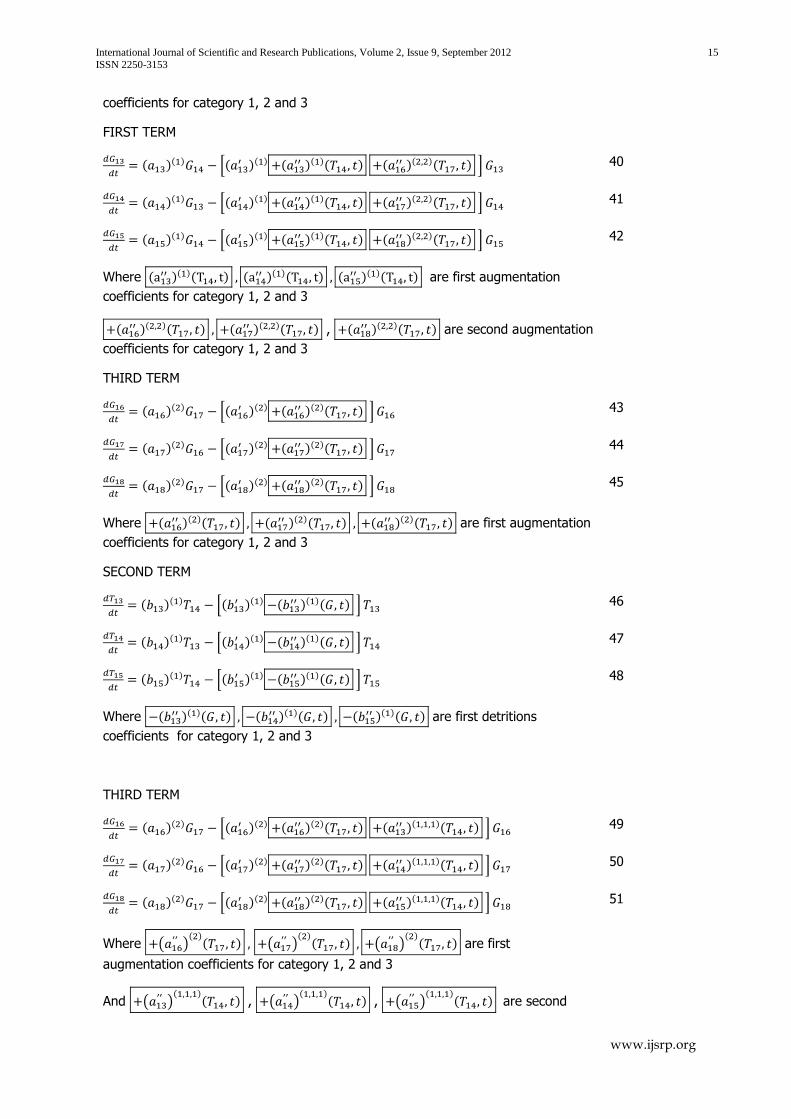
FIRST TERM
( )
( ) 0( )( ) (
)( )( ) ( )( )( ) 1 40
( )
( ) 0( )( ) (
)( )( ) ( )( )( ) 1 41
( )
( ) 0( )( ) (
)( )( ) ( )( )( ) 1 42
Where ( )( )( ) (
)( )( ) ( )( )( ) are first augmentation
coefficients for category 1, 2 and 3
( )( )( ) (
)( )( ) , ( )( )( ) are second augmentation
coefficients for category 1, 2 and 3
THIRD TERM
( )
( ) 0( )( ) (
)( )( ) 1 43
( )
( ) 0( )( ) (
)( )( ) 1 44
( )
( ) 0( )( ) (
)( )( ) 1 45
Where ( )( )( ) (
)( )( ) ( )( )( ) are first augmentation
coefficients for category 1, 2 and 3
SECOND TERM
( )
( ) 0( )( ) (
)( )( ) 1 46
( )
( ) 0( )( ) (
)( )( ) 1 47
( )
( ) 0( )( ) (
)( )( ) 1 48
Where ( )( )( ) (
)( )( ) ( )( )( ) are first detritions
coefficients for category 1, 2 and 3
THIRD TERM
( )
( ) 0( )( ) (
)( )( ) ( )( )( ) 1 49
( )
( ) 0( )( ) (
)( )( ) ( )( )( ) 1 50
( )
( ) 0( )( ) (
)( )( ) ( )( )( ) 1 51
Where ( )
( )( ) (
)( )
( ) ( )
( )( ) are first
augmentation coefficients for category 1, 2 and 3
And ( )
( )( ) , (
)( )
( ) , ( )
( )( ) are second

International Journal of Scientific and Research Publications, Volume 2, Issue 9, September 2012 16
ISSN 2250-3153
www.ijsrp.org
augmentation coefficient for category 1, 2 and 3
SECOND TERM
( )
( ) [( )
( ) (
)( )
( ) ( )
( )( ) ]
52
( )
( ) [( )
( ) (
)( )
( ) ( )
( )( ) ]
53
( )
( ) [( )
( ) (
)( )
( ) ( )
( )( ) ]
54
Where ( )
( )( ) (
)( )
( ) ( )
( )( ) are first detrition
coefficients for category 1, 2 and 3
( )
( )( ) , (
)( )
( ) , ( )
( )( ) are second
detritions coefficient for category 1, 2 and 3
FIRST TERM
( )
( ) [( )
( ) (
)( )
( ) ( )
( )( ) ]
55
( )
( ) [( )
( ) (
)( )
( ) ( )
( )( ) ]
56
( )
( ) [( )
( ) (
)( )
( ) ( )
( )( ) ]
57
Where ( )
( )( ) (
)( )
( ) ( )
( )( ) are first augmentation
coefficients for category 1, 2 and 3
( )
( )( ) , (
)( )
( ) , ( )
( )( ) are second
augmentation coefficient for category 1, 2 and 3
THIRD TERM
( )
( ) [( )
( ) (
)( )
( ) ( )
( )( ) ]
58
( )
( ) [( )
( ) (
)( )
( ) ( )
( )( ) ]
59
( )
( ) [( )
( ) (
)( )
( ) ( )
( )( ) ]
60
( )
( )( ) , (
)( )
( ) , ( )
( )( ) are first detritions
coefficients for category 1, 2 and 3
( )
( )( ) (
)( )
( ) , ( )
( )( ) are second detritions
coefficients for category 1,2 and 3
Uncertainty principle
In quantum mechanics, the uncertainty principle is any of a variety of mathematical inequalities asserting a fundamental lower bound on the precision with which certain pairs of physical

International Journal of Scientific and Research Publications, Volume 2, Issue 9, September 2012 17
ISSN 2250-3153
www.ijsrp.org
properties of a particle, such as position x and momentum p, can be simultaneously known. The
more precisely the position of some particle is determined, the less precisely its momentum can be known, and vice versa The original heuristic argument that such a limit should exist was given
by Werner Heisenberg in 1927. A more formal inequality relating the standard deviation of position σx and the standard deviation of momentum σp was derived by Kennard later that year
(and independently by Weyl in 1928),
Where ħ is the reduced Planck constant.
Historically, the uncertainty principle has been confused with a somewhat similar effect in
physics, called the observer effect which notes that measurements of certain systems cannot be made without affecting the systems. Heisenberg himself offered such an observer effect at the
quantum level (see below) as a physical "explanation" of quantum uncertainty. However, it has
since become clear that quantum uncertainty is inherent in the properties of all wave-like systems, and that it arises in quantum mechanics simply due to the matter wavenature of all
quantum objects. Thus, the uncertainty principle actually states a fundamental property of quantum systems, and is not a statement about the observational success of current technology
Mathematically, the uncertainty relation between position and momentum arises because the
expressions of the wavefunction in the two corresponding bases are Fourier transforms of one another (i.e., position and momentum are conjugate variables). A similar tradeoff between the
variances of Fourier conjugates arises wherever Fourier analysis is needed, for example in sound
waves. A pure tone is a sharp spike at a single frequency. Its Fourier transform gives the shape of the sound wave in the time domain, which is a completely delocalized sine wave. In quantum
mechanics, the two key points are that the position of the particle takes the form of a matter
wave, and momentum is its Fourier conjugate, assured by the de Broglie relation ,
where is the wave number.
In the mathematical formulation of quantum mechanics, any pair of non-commuting self-adjoint operators representing observables are subject to similar uncertainty limits. An eigenstate of an
observable represents the state of the wavefunction for a certain measurement value (the
eigenvalue). For example, if a measurement of an observable is taken then the system is in a
particular eigenstate of that observable. The particular eigenstate of the observable may
not be an eigenstate of another observable . If this is so, then it does not have a single associated measurement as the system is not in an eigenstate of the observable
THE UNCERTAINTY PRINCIPLE:
The uncertainty principle can be interpreted in either the wave mechanics or matrix
mechanics formalisms of quantum mechanics. Although the principle is more visually intuitive in the wave mechanics formalism, it was first derived and is more easily generalized in the matrix
mechanics formalism. We will attempt to motivate the principle in the two frameworks.
Wave mechanics interpretation

International Journal of Scientific and Research Publications, Volume 2, Issue 9, September 2012 18
ISSN 2250-3153
www.ijsrp.org
The superposition of several plane waves. The wave packet becomes increasingly localized with
the addition of many waves. The Fourier transform is a mathematical operation that separates a wave packet into its individual plane waves. Note that the waves shown here are real for
illustrative purposes only whereas in quantum mechanics the wave function is generally complex.
Plane wave
Wave packet
Propagation of de Broglie waves in 1d - real part of the complex amplitude is blue, imaginary
part is green. The probability (shown as the colouropacity) of finding the particle at a given point x is spread out like a waveform, there is no definite position of the particle. As the
amplitude increases above zero the curvature decreases, so the decreases again, and vice versa - the result are alternating amplitude: a wave.

International Journal of Scientific and Research Publications, Volume 2, Issue 9, September 2012 19
ISSN 2250-3153
www.ijsrp.org
According to the de Broglie hypothesis, every object in our Universe is a wave, a situation which
gives rise to this phenomenon. The position of the particle is described by a wave function
. The time-independent wave function of a single-moded plane wave of wave
number k0 or momentum p0 is
The Born rule states that this should be interpreted as a probability density function in the sense
that the probability of finding the particle between a and b is
In the case of the single-moded plane wave, is a uniform distribution. In other words, the particle position is extremely uncertain in the sense that it could be essentially anywhere
along the wave packet. However, consider a wave function that is a sum of many waves. We may write this as
Where An represents the relative contribution of the mode pn to the overall total. The figures to
the right show how with the addition of many plane waves, the wave packet can become more localized. We may take this a step further to the continuum limit, where the wave function is
an integral over all possible modes
With representing the amplitude of these modes and is called the wave function
in momentum space. In mathematical terms, we say that is the Fourier
transforms of and that x and p are conjugate variables. Adding together all of these plane waves comes at a cost, namely the momentum has become less precise, having become a
mixture of waves of many different momenta.
One way to quantify the precision of the position and momentum is the standard deviation σ.
Since is a probability density function for position, we calculate its standard deviation.
We improved the precision of the position, i.e. reduced σx, by using many plane waves, thereby
weakening the precision of the momentum, i.e. increased σp. Another way of stating this is that σx and σp has an inverse relationship or are at least bounded from below. This is the uncertainty
principle, the exact limit of which is the Kennard bound. Click the show button below to see a semi-formal derivation of the Kennard inequality using wave mechanics.
Matrix mechanics interpretation
In matrix mechanics, observables such as position and momentum are represented by self-
adjoint operators. When considering pairs of observables, one of the most important quantities is
the commutator. For a pair of operators and , we may define their commutator as
In the case of position and momentum, the commutator is the canonical commutation relation

International Journal of Scientific and Research Publications, Volume 2, Issue 9, September 2012 20
ISSN 2250-3153
www.ijsrp.org
The physical meaning of the non-commutativity can be understood by considering the effect of
the commutator on position and momentum eigenstates. Let be a right eigenstate of
position with a constant eigenvalue x0. By definition, this means that
Applying the commutator to yields
where is simply the identity operator. Suppose for the sake of proof by contradiction that
is also a right eigenstate of momentum, with constant eigenvalue p0. If this were true, then we
could write
On the other hand, the canonical commutation relation requires that
This implies that no quantum state can be simultaneously both a position and a momentum eigenstate. When a state is measured, it is projected onto an eigenstate in the basis of the
observable. For example, if a particle's position is measured, then the state exists at least
momentarily in a position eigenstate. However, this means that the state is not in a momentum eigenstate but rather exists as a sum of multiple momentum basis eigenstates. In other words
the momentum must be less precise. The precision may be quantified by the standard deviations, defined by
As with the wave mechanics interpretation above, we see a tradeoff between the precisions of
the two, given by the uncertainty principle.
Robertson-Schrödinger uncertainty relations
The most common general form of the uncertainty principle is the Robertson uncertainty
relation. For an arbitrary Hermitian operator , we can associate a standard deviation
Where the brackets indicate an expectation value. For a pair of operators and , we
may define their commutator as
In this notation, the Robertson uncertainty relation is given by
he Robertson uncertainty relation immediately follows from a slightly stronger inequality,
International Journal of Scientific and Research Publications, Volume 2, Issue 9, September 2012 21
ISSN 2250-3153
www.ijsrp.org
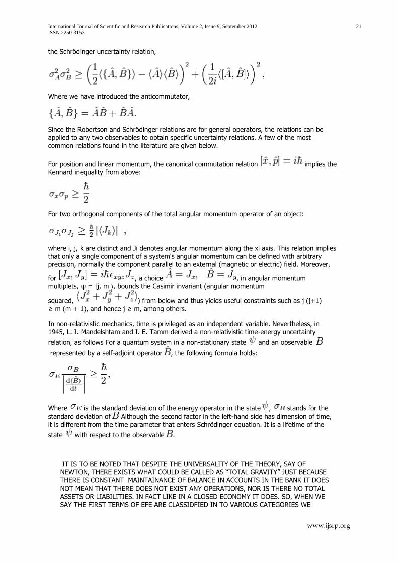
the Schrödinger uncertainty relation,
Where we have introduced the anticommutator,
Since the Robertson and Schrödinger relations are for general operators, the relations can be applied to any two observables to obtain specific uncertainty relations. A few of the most
common relations found in the literature are given below.
For position and linear momentum, the canonical commutation relation implies the
Kennard inequality from above:
For two orthogonal components of the total angular momentum operator of an object:
where i, j, k are distinct and Ji denotes angular momentum along the xi axis. This relation implies
that only a single component of a system's angular momentum can be defined with arbitrary precision, normally the component parallel to an external (magnetic or electric) field. Moreover,
for , a choice , in angular momentum multiplets, ψ = |j, m ⟩, bounds the Casimir invariant (angular momentum
squared, ) from below and thus yields useful constraints such as j (j+1)
≥ m (m + 1), and hence j ≥ m, among others.
In non-relativistic mechanics, time is privileged as an independent variable. Nevertheless, in 1945, L. I. Mandelshtam and I. E. Tamm derived a non-relativistic time-energy uncertainty
relation, as follows For a quantum system in a non-stationary state and an observable
represented by a self-adjoint operator , the following formula holds:
Where is the standard deviation of the energy operator in the state , stands for the
standard deviation of Although the second factor in the left-hand side has dimension of time,
it is different from the time parameter that enters Schrödinger equation. It is a lifetime of the
state with respect to the observable .
IT IS TO BE NOTED THAT DESPITE THE UNIVERSALITY OF THE THEORY, SAY OF NEWTON, THERE EXISTS WHAT COULD BE CALLED AS ―TOTAL GRAVITY‖ JUST BECAUSE
THERE IS CONSTANT MAINTAINANCE OF BALANCE IN ACCOUNTS IN THE BANK IT DOES NOT MEAN THAT THERE DOES NOT EXIST ANY OPERATIONS, NOR IS THERE NO TOTAL
ASSETS OR LIABILITIES. IN FACT LIKE IN A CLOSED ECONOMY IT DOES. SO, WHEN WE
SAY THE FIRST TERMS OF EFE ARE CLASSIDFIED IN TO VARIOUS CATEGORIES WE

International Journal of Scientific and Research Publications, Volume 2, Issue 9, September 2012 22
ISSN 2250-3153
www.ijsrp.org
REFER TO THE FACT THAT VARIOUS SYSTEMS ARE UNDER CONSIDERATION AND THEY
OFCOURSE SATISFY GTR. THE SAME EXPLANTION HOLDS GOOD IN THE STARTIFICATION OF THE HEISENBERG‘S PRINCIPLE OF UNCERTAINTY. FIRST, WE
DISCUSS THE EQUALITY CASE. WE TRANSFER THETERM REPRESENTATIVE OF POSITION OF PARTICLE OR THE ONE CONSTITUTIVE OF MONEMTUM TO THE OTHER SIDE AND THE
RELATIONSHIP THAT EXISTS NOW BETWIXT ―POSITION‖ AND MOMENTUM IS THAT THE
INVERSE OF ONE IS BEING ―SUBTRACTED ―FROM THE OTHER. THIS APPARANTELY MEANS THAT ONE TERM IS BEITAKEN OUT FROM THE OTHER. THERE MAY OR MIGHT
NOT BE TIME LAG. THAT DOES NOT MATTYER IN OPUR CALCULATION. THE EQUATIONS REPRESENT AND CONSTITUTE THE GLOBALISED EQUATIONS WHICH IS BASED ON THE
SIMPLE MATTER OF ACCENTUATION AND DISSSIPATION. IN FACT THE FUNCTIONAL FORMS OF ACCENTUATION AND DISSIPATION TERMS THEMSELVES ARE DESIGNATIVE
OF THE FACT THAT THERE EXISTS A LINK BETWEEN THE VARIOUS THEORIES GALILEAN,
PLATONIC, MENTAL, GTR, STR, QM.QFT, AND QUANTUM GRAVITY. FINALLY. I AN SERIES OF PAPER WE SHALL BUILD UP THE STRUCTURE TOWARDS THE END OF
CONSUMMATION OF THE UNIFICATION OF THE THEORIES. THAT OINE THEORY IS RELATED TO ANOTHER IS BEYOND DISPUTE AND WE TAKE OFF FROM THAT POINT
TOWARDS OUR MISSION.
FIRST TERM AND SECOND TERM IN EFE :
==========================================================================
: CATEGORY ONE OF THE FIRST TERM IN EFE
: CATEGORY TWO OF THE FIRST TERM IN EFE
: CATEGORY THREEOF FIRST TERM IN EFE
: CATEGORY ONE OF SECOND TERM IN EFE
: CATEGORY TWO OF THE SECOND TERM IN EFE
: CATEGORY THREE OF SECOND TERM IN EFE
THIRD TERM AND FOURTH TERM OF EFE: NOTE FOURTH TERM ON RHS IS REMOVED FROM THE THIRD TERM
==========================================================
================
: CATEGORY ONE OF THIRD TERM OF EFE
: CATEGORY TWO OF THIRD TERM OF EFE
: CATEGORY THREE OF THIRD TERM OF EFE
: CATEGORY ONE OF FOURTH TERM OF EFE
: CATEGORY TWO OF FOURTH TERM OF EFE
: CATEGORY THREE OF FOURTH TERM OF EFE
1

International Journal of Scientific and Research Publications, Volume 2, Issue 9, September 2012 23
ISSN 2250-3153
www.ijsrp.org
HEISENBERG‘S UNCERTAINTY PRINCIPLE:
NOTE THE FIRST TERM IS INVERSELY PROPORTIONAL TO THE SECOND TERM. TAKE THE EQUALITY CASE. THIS LEADS TO SUBTRACTION OF THE SECOND TERM ON THE RHS FROM
THE FIRST TERM THIS WWE SHALL MODEL AND ANNEX WITH EFE. DESPITE HUP HOLDING GOOD FOR ALL THE SYSTEMS, WE CAN CLASSIFY THE SYSTEMS STUDIED AND NOTE THE
REGISTRATIONS IN EACH SYSTEM. AS SAID EARLIER THE FIRST TERM VALUE OF SOME
SYSTEM, THE SECOND TERM VALUE OF SOME OTHER DIFFERENTIATION CARRIED OUT BASED ON PARAMETRICIZATION
==========================================================
==============
: CATEGORY ONE OF FIRST TERM ON HUP
: CATEGORY TWO OF FIRST TERM OF HUP
: CATEGORY THREE OF FIRST TERM OF HUP
: CATEGORY ONE OF SECOND TERM OF HUP
: CATEGORY TWO OF SECOND TERM OF UCP
: CATEGORY THREE OF SECOND TERM OF HUP
ACCENTUATION COEFFCIENTS:OF HOLISTIC SYSTEM EFE-HUP SYSTEM
==========================================================
================
( )( ) ( )
( ) ( )( ) ( )
( ) ( )( ) ( )
( ) ( )( ) ( )
( ) ( )( )
( )( ) ( )
( ) ( )( ): ( )
( ) ( )( ) ( )
( ) ( )( ) ( )
( ) ( )( )
===========================================================================
( )
( ) (
)( )
( )
( ) (
)( )
( )
( ) (
)( )
( )
( ) (
)( )
( )
( )
( )
( ) (
)( )
( )
( ) (
)( )
( )
( ) (
)( )
( )
( ) (
)( )
( )
( )
FIRST TERM OF EFE- SECOND TERM OF EFE:GOVERNING EQUATIONS:
The differential system of this model is now
( )
( ) 0( )
( ) (
)( )
( )1
( )
( ) 0( )
( ) (
)( )
( )1 1
( )
( ) 0( )
( ) (
)( )
( )1 2
( )
( ) 0( )
( ) (
)( )
( )1 3
( )
( ) 0( )
( ) (
)( )
( )1 4

International Journal of Scientific and Research Publications, Volume 2, Issue 9, September 2012 24
ISSN 2250-3153
www.ijsrp.org
( )
( ) 0( )
( ) (
)( )
( )1 5
( )
( )( ) First augmentation factor
( )
( )( ) First detritions factor 6
GOVERNING EQUATIONS:THIRD TERM OF EFE AND FOURTH TERM OF EFE:
The differential system of this model is now
7
( )
( ) 0( )
( ) (
)( )
( )1 8
( )
( ) 0( )
( ) (
)( )
( )1 9
( )
( ) 0( )
( ) (
)( )
( )1 10
( )
( ) 0( )
( ) (
)( )
(( ) )1 11
( )
( ) 0( )
( ) (
)( )
(( ) )1 12
( )
( ) 0( )
( ) (
)( )
(( ) )1 13
( )( )( ) First augmentation factor 14
( )( )(( ) ) First detritions factor 15
GOVERNING EQUATIONS:OF THE FIRST TERM AND SECOND TERM OF HUP:NOTE
THAT FSECOND TERM (INVERSE THEREOF) IS SUBTRACTED FROM THE FIRST TERM ,WHICH MEANS THE AMOUNT IS REMOVED FOR INFINITE SYSTEMS IN THE
WORLD. LAW OFCOURSE HOLDS FOR ALL THE SYSTEMS BY THIS METHIODLOGY WE GET THE VALUE OF THE FIRST TERM AS WELL AS THE SECOND TERM
=========================================================================
The differential system of this model is now
16
( )
( ) [( )( ) (
)( )( )] 17
( )
( ) [( )( ) (
)( )( )] 18
( )
( ) [( )( ) (
)( )( )] 19
( )
( ) [( )( ) (
)( )( )] 20
( )
( ) [( )( ) (
)( )( )] 21

International Journal of Scientific and Research Publications, Volume 2, Issue 9, September 2012 25
ISSN 2250-3153
www.ijsrp.org
( )
( ) [( )( ) (
)( )( )] 22
( )( )( ) First augmentation factor 23
( )( )( ) First detritions factor 24
25
GOVERNING EQUATIONS OF THE HOLISTIC SYSTEM FOUR TERMS OF EFE AND TWO TERMS
OF HUP:
====================================================================================
26
( )
( ) 0( )( ) (
)( )( ) ( )( )( ) (
)( )( ) 1 27
( )
( ) 0( )( ) (
)( )( ) ( )( )( ) (
)( )( ) 1 28
( )
( ) 0( )( ) (
)( )( ) ( )( )( ) (
)( )( ) 1 29
Where ( )( )( ) (
)( )( ) ( )( )( ) are first augmentation coefficients for
category 1, 2 and 3
( )( )( ) , (
)( )( ) , ( )( )( ) are second augmentation
coefficient for category 1, 2 and 3
( )( )( ) (
)( )( ) ( )( )( ) are third augmentation coefficient
for category 1, 2 and 3
30
31
( )
( ) 0( )( ) (
)( )( ) ( )( )( ) (
)( )( ) 1 32
( )
( ) 0( )( ) (
)( )( ) ( )( )( ) (
)( )( ) 1 33
( )
( ) 0( )( ) (
)( )( ) ( )( )( ) (
)( )( ) 1 34
Where ( )( )( ) (
)( )( ) ( )( )( ) are first detrition coefficients for
category 1, 2 and 3
( )( )( ) (
)( )( ) ( )( )( ) are second detrition coefficients for
category 1, 2 and 3
( )( )( ) (
)( )( ) ( )( )( ) are third detrition coefficients for
35
International Journal of Scientific and Research Publications, Volume 2, Issue 9, September 2012 26
ISSN 2250-3153
www.ijsrp.org
category 1, 2 and 3
( )
( ) 0( )( ) (
)( )( ) ( )( )( ) (
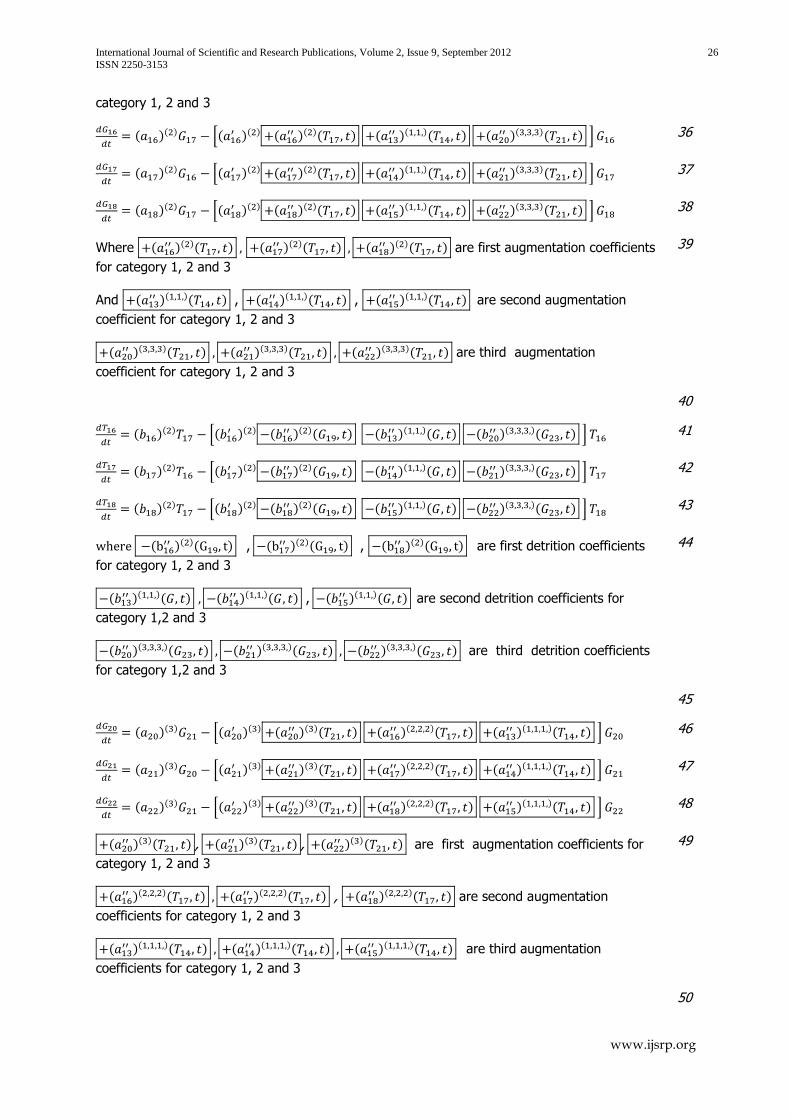
)( )( ) 1 36
( )
( ) 0( )( ) (
)( )( ) ( )( )( ) (
)( )( ) 1 37
( )
( ) 0( )( ) (
)( )( ) ( )( )( ) (
)( )( ) 1 38
Where ( )( )( ) (
)( )( ) ( )( )( ) are first augmentation coefficients
for category 1, 2 and 3
And ( )( )( ) , (
)( )( ) , ( )( )( ) are second augmentation
coefficient for category 1, 2 and 3
( )( )( ) (
)( )( ) ( )( )( ) are third augmentation
coefficient for category 1, 2 and 3
39
40
( )
( ) 0( )( ) (
)( )( ) ( )( )( ) (
)( )( ) 1 41
( )
( ) 0( )( ) (
)( )( ) ( )( )( ) (
)( )( ) 1 42
( )
( ) 0( )( ) (
)( )( ) ( )( )( ) (
)( )( ) 1 43
( )( )( ) , (
)( )( ) , ( )( )( ) are first detrition coefficients
for category 1, 2 and 3
( )( )( ) (
)( )( ) , ( )( )( ) are second detrition coefficients for
category 1,2 and 3
( )( )( ) (
)( )( ) ( )( )( ) are third detrition coefficients
for category 1,2 and 3
44
45
( )
( ) 0( )( ) (
)( )( ) ( )( )( ) (
)( )( ) 1 46
( )
( ) 0( )( ) (
)( )( ) ( )( )( ) (
)( )( ) 1 47
( )
( ) 0( )( ) (
)( )( ) ( )( )( ) (
)( )( ) 1 48
( )( )( ) , (
)( )( ) , ( )( )( ) are first augmentation coefficients for
category 1, 2 and 3
( )( )( ) (
)( )( ) , ( )( )( ) are second augmentation
coefficients for category 1, 2 and 3
( )( )( ) (
)( )( ) ( )( )( ) are third augmentation
coefficients for category 1, 2 and 3
49
50

International Journal of Scientific and Research Publications, Volume 2, Issue 9, September 2012 27
ISSN 2250-3153
www.ijsrp.org
( )
( ) 0( )( ) (
)( )( ) ( )( )( ) (
)( )( ) 1 51
( )
( ) 0( )( ) (
)( )( ) ( )( )( ) (
)( )( ) 1 52
( )
( ) 0( )( ) (
)( )( ) ( )( )( ) (
)( )( ) 1 53
( )( )( ) (
)( )( ) ( )( )( ) are first detrition coefficients for
category 1, 2 and 3
( )( )( ) , (
)( )( ) , ( )( )( ) are second detrition coefficients
for category 1, 2 and 3
( )( )( ) (
)( )( ) , ( )( )( ) are third detrition coefficients for
category 1,2 and 3
54
55
Where we suppose 56
(A) ( )( ) (
)( ) ( )( ) ( )
( ) ( )( ) (
)( )
(B) The functions ( )( ) (
)( ) are positive continuous increasing and bounded.
Definition of ( )( ) ( )
( ):
( )( )( ) ( )
( ) ( )( )
( )( )( ) ( )
( ) ( )( ) ( )
( )
57
(C) ( )( ) ( ) ( )
( )
( )( ) ( ) ( )
( )
Definition of ( )( ) ( )
( ) :
Where ( )( ) ( )
( ) ( )( ) ( )
( ) are positive constants
and
58
They satisfy Lipschitz condition:
( )( )(
) ( )( )( ) ( )
( ) ( )
( )
( )( )( ) (
)( )( ) ( )( ) ( )
( )
59
60
61
With the Lipschitz condition, we place a restriction on the behavior of functions
( )( )(
) and( )( )( ) (
) and ( ) are points belonging to the interval
[( )( ) ( )
( )] . It is to be noted that ( )( )( ) is uniformly continuous. In the
eventuality of the fact, that if ( )( ) then the function (
)( )( ) , the first
augmentation coefficient WOULD BE absolutely continuous.
62
Definition of ( )( ) ( )
( ) :
(D) ( )( ) ( )
( ) are positive constants
63

International Journal of Scientific and Research Publications, Volume 2, Issue 9, September 2012 28
ISSN 2250-3153
www.ijsrp.org
( )
( )
( )( )
( )( )
( )( )
Definition of ( )( ) ( )
( ) :
(E) There exists two constants ( )( ) and ( )
( ) which together with
( )( ) ( )
( ) ( )( ) ( )
( ) and the constants
( )( ) (
)( ) ( )( ) (
)( ) ( )( ) ( )
( )
satisfy the inequalities
( )( ) , ( )
( ) ( )( ) ( )
( ) ( )( ) ( )
( )-
( )( ) , ( )
( ) ( )( ) ( )
( ) ( )( ) ( )
( )-
64
65
66
67
68
Where we suppose 69
(F) ( )( ) (
)( ) ( )( ) ( )
( ) ( )( ) (
)( ) 70
(G) The functions ( )( ) (
)( ) are positive continuous increasing and bounded. 71
Definition of ( )( ) ( )
( ): 72
( )( )( ) ( )
( ) ( )( )
73
( )( )( ) ( )
( ) ( )( ) ( )
( ) 74
(H) ( )( ) ( ) ( )
( ) 75
( )( ) (( ) ) ( )
( ) 76
Definition of ( )( ) ( )
( ) :
Where ( )( ) ( )
( ) ( )( ) ( )
( ) are positive constants and
77
They satisfy Lipschitz condition: 78
( )( )(
) ( )( )( ) ( )
( ) ( )
( ) 79
( )( )(( )
) ( )( )(( ) ) ( )
( ) ( ) ( ) ( )
( ) 80
With the Lipschitz condition, we place a restriction on the behavior of functions ( )( )(
)
and( )( )( ) . (
) and ( ) are points belonging to the interval [( )( ) ( )
( )]
. It is to be noted that ( )( )( ) is uniformly continuous. In the eventuality of the fact, that
if ( )( ) then the function (
)( )( ) , the SECOND augmentation coefficient
attributable to would be absolutely continuous.
81
Definition of ( )( ) ( )
( ) : 82
(I) ( )( ) ( )
( ) are positive constants
( )
( )
( )( )
( )( )
( )( )
83
Definition of ( )( ) ( )
( ) :
There exists two constants ( )( ) and ( )
( ) which together
with ( )( ) ( )
( ) ( )( ) ( )
( ) and the constants
84

International Journal of Scientific and Research Publications, Volume 2, Issue 9, September 2012 29
ISSN 2250-3153
www.ijsrp.org
( )( ) (
)( ) ( )( ) (
)( ) ( )( ) ( )
( )
satisfy the inequalities
( )( ) , ( )
( ) ( )( ) ( )
( ) ( )( ) ( )
( )- 85
( )( ) , ( )
( ) ( )( ) ( )
( ) ( )( ) ( )
( )- 86
Where we suppose 87
(J) ( )( ) (
)( ) ( )( ) ( )
( ) ( )( ) (
)( )
(K) The functions ( )( ) (
)( ) are positive continuous increasing and bounded.
Definition of ( )( ) ( )
( ):
( )( )( ) ( )
( ) ( )( )
( )( )( ) ( )
( ) ( )( ) ( )
( )
88
(L) ( )( ) ( ) ( )
( )
( )( ) ( ) ( )
( )
Definition of ( )( ) ( )
( ) :
Where ( )( ) ( )
( ) ( )( ) ( )
( ) are positive constants and
89
90
91
They satisfy Lipschitz condition:
( )( )(
) ( )( )( ) ( )
( ) ( )
( )
( )( )(
) ( )( )( ) ( )
( ) ( )
( )
92
93
94
With the Lipschitz condition, we place a restriction on the behavior of functions ( )( )(
)
and( )( )( ) . (
) And ( ) are points belonging to the interval [( )( ) ( )
( )]
. It is to be noted that ( )( )( ) is uniformly continuous. In the eventuality of the fact, that
if ( )( ) then the function (
)( )( ) , the THIRD augmentation coefficient would
be absolutely continuous.
95
Definition of ( )( ) ( )
( ) :
(M) ( )( ) ( )
( ) are positive constants
( )
( )
( )( )
( )( )
( )( )
96
There exists two constants There exists two constants ( )( ) and ( )
( ) which together
with ( )( ) ( )
( ) ( )( ) ( )
( ) and the constants
( )( ) (
)( ) ( )( ) (
)( ) ( )( ) ( )
( )
satisfy the inequalities
( )( ) , ( )
( ) ( )( ) ( )
( ) ( )( ) ( )
( )-
97
98
99
100
International Journal of Scientific and Research Publications, Volume 2, Issue 9, September 2012 30
ISSN 2250-3153
www.ijsrp.org
( )( ) , ( )
( ) ( )( ) ( )
( ) ( )( ) ( )
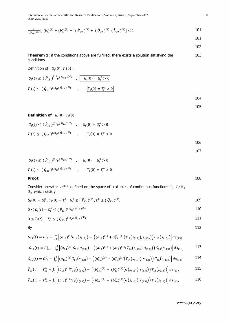
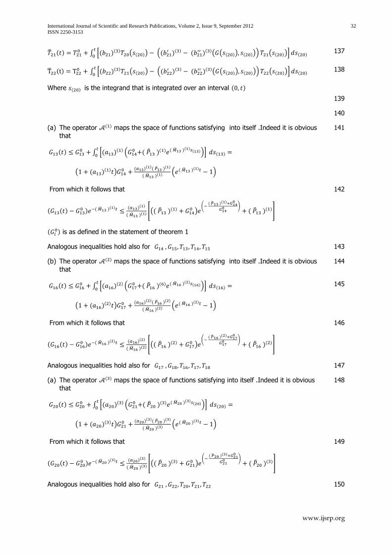
( )- 101
101
102
Theorem 1: if the conditions above are fulfilled, there exists a solution satisfying the conditions
Definition of ( ) ( ) :
( ) ( )( )
( )( ) , ( )
( ) ( )( ) ( )
( ) , ( )
103
104
Definition of ( ) ( )
( ) ( )( ) ( )
( ) , ( )
( ) ( )( ) ( )
( ) , ( )
105
106
( ) ( )( ) ( )
( ) , ( )
( ) ( )( ) ( )
( ) , ( )
107
Proof:
Consider operator ( ) defined on the space of sextuples of continuous functions which satisfy
108
( ) ( )
( )
( ) ( )
( ) 109
( ) ( )
( ) ( )( ) 110
( ) ( )
( ) ( )( ) 111
By
( ) ∫ 0( )
( ) ( ( )) .( )( )
)( )( ( ( )) ( ))/ ( ( ))1 ( )
112
( ) ∫ 0( )
( ) ( ( )) .( )( ) (
)( )( ( ( )) ( ))/ ( ( ))1 ( )
113
( ) ∫ 0( )
( ) ( ( )) .( )( ) (
)( )( ( ( )) ( ))/ ( ( ))1 ( )
114
( ) ∫ 0( )
( ) ( ( )) .( )( ) (
)( )( ( ( )) ( ))/ ( ( ))1 ( )
115
( ) ∫ 0( )
( ) ( ( )) .( )( ) (
)( )( ( ( )) ( ))/ ( ( ))1 ( )
116

International Journal of Scientific and Research Publications, Volume 2, Issue 9, September 2012 31
ISSN 2250-3153
www.ijsrp.org
( ) ∫ 0( )
( ) ( ( )) .( )( ) (
)( )( ( ( )) ( ))/ ( ( ))1 ( )
Where ( ) is the integrand that is integrated over an interval ( )
117
118
Proof:
Consider operator ( ) defined on the space of sextuples of continuous functions which satisfy
119
( ) ( )
( )
( ) ( )
( ) 120
( ) ( )
( ) ( )( ) 121
( ) ( )
( ) ( )( ) 122
By
( ) ∫ 0( )
( ) ( ( )) .( )( )
)( )( ( ( )) ( ))/ ( ( ))1 ( )
123
( ) ∫ 0( )
( ) ( ( )) .( )( ) (
)( )( ( ( )) ( ))/ ( ( ))1 ( )
124
( ) ∫ 0( )
( ) ( ( )) .( )( ) (
)( )( ( ( )) ( ))/ ( ( ))1 ( )
125
( ) ∫ 0( )
( ) ( ( )) .( )( ) (
)( )( ( ( )) ( ))/ ( ( ))1 ( )
126
( ) ∫ 0( )
( ) ( ( )) .( )( ) (
)( )( ( ( )) ( ))/ ( ( ))1 ( )
127
( ) ∫ 0( )
( ) ( ( )) .( )( ) (
)( )( ( ( )) ( ))/ ( ( ))1 ( )
Where ( ) is the integrand that is integrated over an interval ( )
128
Proof:
Consider operator ( ) defined on the space of sextuples of continuous functions which satisfy
129
( ) ( )
( )
( ) ( )
( ) 130
( ) ( )
( ) ( )( ) 131
( ) ( )
( ) ( )( ) 132
By
( ) ∫ 0( )
( ) ( ( )) .( )( )
)( )( ( ( )) ( ))/ ( ( ))1 ( )
133
( ) ∫ 0( )
( ) ( ( )) .( )( ) (
)( )( ( ( )) ( ))/ ( ( ))1 ( )
134
( ) ∫ 0( )
( ) ( ( )) .( )( ) (
)( )( ( ( )) ( ))/ ( ( ))1 ( )
135
( ) ∫ 0( )
( ) ( ( )) .( )( ) (
)( )( ( ( )) ( ))/ ( ( ))1 ( )
136
International Journal of Scientific and Research Publications, Volume 2, Issue 9, September 2012 32
ISSN 2250-3153
www.ijsrp.org
( ) ∫ 0( )
( ) ( ( )) .( )( ) (
)( )( ( ( )) ( ))/ ( ( ))1 ( )
137
( ) ∫ 0( )
( ) ( ( )) .( )( ) (
)( )( ( ( )) ( ))/ ( ( ))1 ( )
Where ( ) is the integrand that is integrated over an interval ( )
138
139
140
(a) The operator ( ) maps the space of functions satisfying into itself .Indeed it is obvious
that
( ) ∫ 0( )
( ) . ( )
( ) ( )( ) ( )/1
( )
( ( )( ) )
( )
( )( )( )
( )( ) . ( )
( ) /
141
From which it follows that
( ( ) ) ( )
( ) ( )
( )
( )( ) [(( )
( ) )
( ( )( )
)
( )( )]
( ) is as defined in the statement of theorem 1
142
Analogous inequalities hold also for 143
(b) The operator ( ) maps the space of functions satisfying into itself .Indeed it is obvious
that
144
( ) ∫ 0( )
( ) . ( )
( ) ( )( ) ( )/1
( )
( ( )( ) )
( )
( )( )( )
( )( ) . ( )
( ) /
145
From which it follows that
( ( ) ) ( )
( ) ( )
( )
( )( ) [(( )
( ) )
( ( )( )
)
( )( )]
146
Analogous inequalities hold also for 147
(a) The operator ( ) maps the space of functions satisfying into itself .Indeed it is obvious
that
( ) ∫ 0( )
( ) . ( )
( ) ( )( ) ( )/1
( )
( ( )( ) )
( )
( )( )( )
( )( ) . ( )
( ) /
148
From which it follows that
( ( ) ) ( )
( ) ( )
( )
( )( ) [(( )
( ) )
( ( )( )
)
( )( )]
149
Analogous inequalities hold also for 150

International Journal of Scientific and Research Publications, Volume 2, Issue 9, September 2012 33
ISSN 2250-3153
www.ijsrp.org
151
It is now sufficient to take ( )
( )
( )( )
( )( )
( )( ) and to choose
( )( ) ( )
( ) large to have
152
( )( )
( )( ) [( )
( ) (( )( )
) (
( )( )
)
] ( )( )
153
( )( )
( )( ) [(( )
( ) )
( ( )
( )
)
( )( )] ( )
( )
154
In order that the operator ( ) transforms the space of sextuples of functions into itself 155
The operator ( ) is a contraction with respect to the metric
.( ( ) ( )) ( ( ) ( ))/
*
| ( )( )
( )( )| ( )( )
|
( )( ) ( )( )| ( )
( ) +
156
Indeed if we denote
Definition of :
( ) ( )( )
It results
| ( )
( )| ∫ ( )( )
|
( ) ( )| ( )
( ) ( ) ( )( ) ( ) ( )
∫ *( )( )|
( ) ( )| ( )
( ) ( ) ( )( ) ( )
( )( )(
( ) ( ))| ( )
( )| ( )( ) ( ) ( )
( ) ( )
( ) (
)( )( ( ) ( )) (
)( )( ( ) ( ))
( )( ) ( ) ( )
( ) ( )+ ( )
Where ( ) represents integrand that is integrated over the interval , -
From the hypotheses it follows
157
| ( ) ( )| ( )( )
( )( ) (( )
( ) ( )( ) ( )
( ) ( )( )( )
( )) .( ( ) ( ) ( ) ( ))/
And analogous inequalities for . Taking into account the hypothesis the result follows
158
Remark 1: The fact that we supposed ( )( ) (
)( ) depending also on can be
considered as not conformal with the reality, however we have put this hypothesis ,in order
that we can postulate condition necessary to prove the uniqueness of the solution bounded by
( )( ) ( )
( ) ( )( ) ( )
( ) respectively of
159
International Journal of Scientific and Research Publications, Volume 2, Issue 9, September 2012 34
ISSN 2250-3153
www.ijsrp.org
If instead of proving the existence of the solution on , we have to prove it only on a
compact then it suffices to consider that ( )( ) (
)( ) depend only on and respectively on ( ) and hypothesis can replaced by a usual Lipschitz
condition.
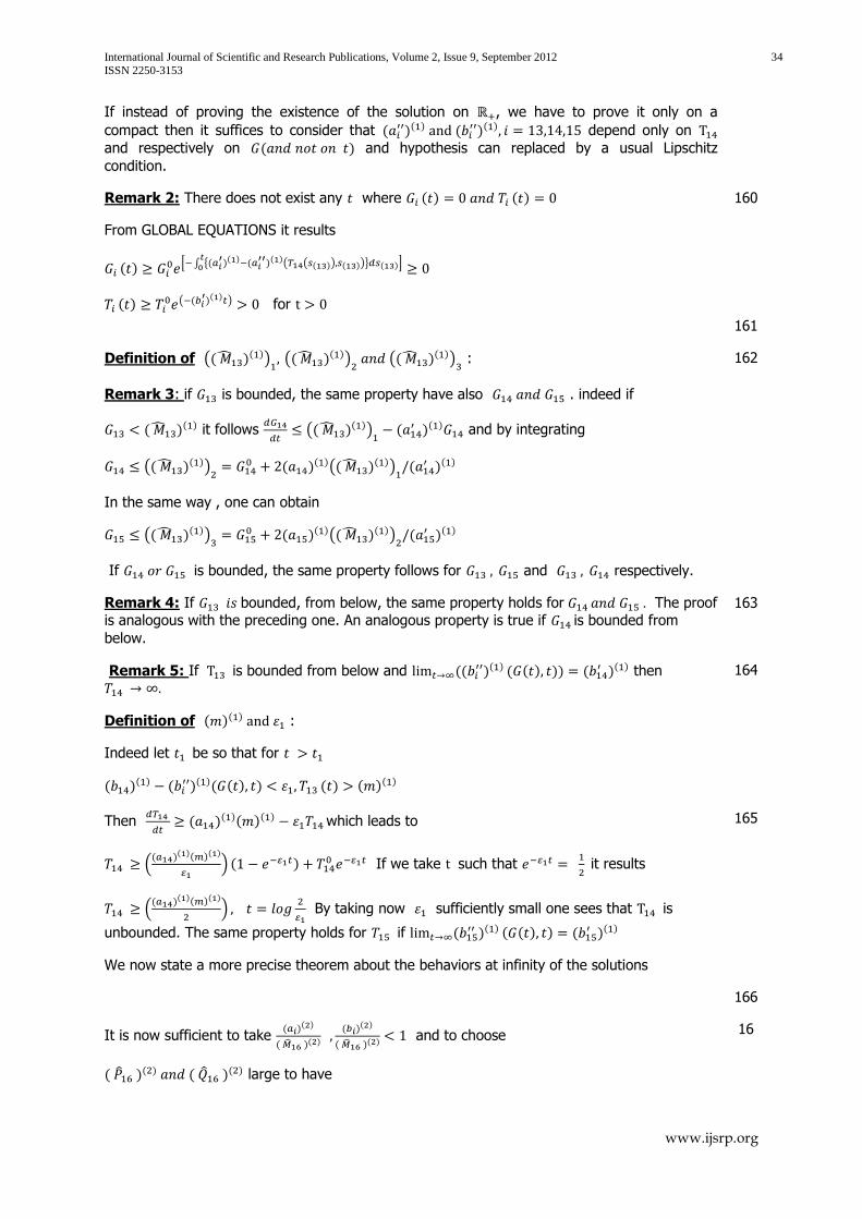
Remark 2: There does not exist any where ( ) ( )
From GLOBAL EQUATIONS it results
( ) 0 ∫ {(
)( ) ( )( )( ( ( )) ( ))} ( )
1
( ) ( (
)( ) ) for
160
161
Definition of (( )( ))
(( )
( )) (( )
( )) :
Remark 3: if is bounded, the same property have also . indeed if
( )( ) it follows
(( )
( )) (
)( ) and by integrating
(( )( ))
( )( )(( )
( )) (
)( )
In the same way , one can obtain
(( )( ))
( )( )(( )
( )) (
)( )
If is bounded, the same property follows for and respectively.
162
Remark 4: If bounded, from below, the same property holds for The proof
is analogous with the preceding one. An analogous property is true if is bounded from
below.
163
Remark 5: If is bounded from below and (( )( ) ( ( ) )) (
)( ) then
Definition of ( )( ) :
Indeed let be so that for
( )( ) (
)( )( ( ) ) ( ) ( )( )
164
Then
( )
( )( )( ) which leads to
.( )
( )( )( )
/ ( )
If we take such that
it results
.( )
( )( )( )
/
By taking now sufficiently small one sees that is
unbounded. The same property holds for if ( )( ) ( ( ) ) (
)( )
We now state a more precise theorem about the behaviors at infinity of the solutions
165
166
It is now sufficient to take ( )
( )
( )( )
( )( )
( )( ) and to choose
( )( ) ( )
( ) large to have
16

International Journal of Scientific and Research Publications, Volume 2, Issue 9, September 2012 35
ISSN 2250-3153
www.ijsrp.org
( )( )
( )( ) [( )
( ) (( )( )
) (
( )( )
)
] ( )( )
7
( )( )
( )( ) [(( )
( ) )
( ( )
( )
)
( )( )] ( )
( )
168
In order that the operator ( ) transforms the space of sextuples of functions into itself 169
The operator ( ) is a contraction with respect to the metric
.(( )( ) ( )
( )) (( )( ) ( )
( ))/
*
| ( )( )
( )( )| ( )( )
|
( )( ) ( )( )| ( )
( ) +
170
171
Indeed if we denote
Definition of :
( ) ( )( )
172
It results
| ( )
( )| ∫ ( )( )
|
( ) ( )| ( )
( ) ( ) ( )( ) ( ) ( )
∫ *( )( )|
( ) ( )| ( )
( ) ( ) ( )( ) ( )
( )( )(
( ) ( ))| ( )
( )| ( )( ) ( ) ( )
( ) ( )
( ) (
)( )( ( ) ( )) (
)( )( ( ) ( ))
( )( ) ( ) ( )
( ) ( )+ ( )
173
Where ( ) represents integrand that is integrated over the interval , -
From the hypotheses it follows
174
|( )( ) ( )
( )| ( )( )
( )( ) (( )
( ) ( )( ) ( )
( )
( )( )( )
( )) .(( )( ) ( )
( ) ( )( ) ( )
( ))/
175
And analogous inequalities for . Taking into account the hypothesis the result follows 176
Remark 1: The fact that we supposed ( )( ) (
)( ) depending also on can be
considered as not conformal with the reality, however we have put this hypothesis ,in order that we can postulate condition necessary to prove the uniqueness of the solution bounded by
( )( ) ( )
( ) ( )( ) ( )
( ) respectively of
If instead of proving the existence of the solution on , we have to prove it only on a
compact then it suffices to consider that ( )( ) (
)( ) depend only on and respectively on ( )( ) and hypothesis can replaced by a usual Lipschitz
177
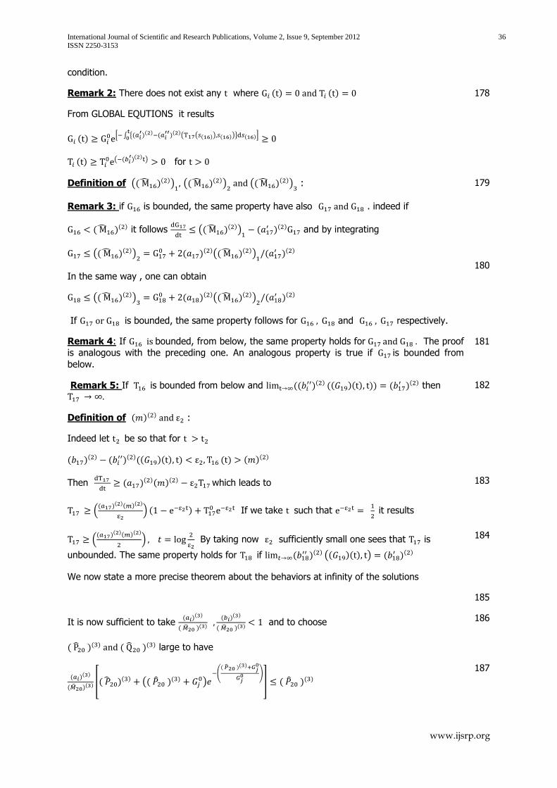
International Journal of Scientific and Research Publications, Volume 2, Issue 9, September 2012 36
ISSN 2250-3153
www.ijsrp.org
condition.
Remark 2: There does not exist any where ( ) ( )
From GLOBAL EQUTIONS it results
( ) 0 ∫ {(
)( ) ( )( )( ( ( )) ( ))} ( )
1
( ) ( (
)( ) ) for
178
Definition of (( )( ))
(( )
( )) (( )
( )) :
Remark 3: if is bounded, the same property have also . indeed if
( )( ) it follows
(( )
( )) (
)( ) and by integrating
(( )( ))
( )( )(( )
( )) (
)( )
In the same way , one can obtain
(( )( ))
( )( )(( )
( )) (
)( )
If is bounded, the same property follows for and respectively.
179
180
Remark 4: If bounded, from below, the same property holds for The proof
is analogous with the preceding one. An analogous property is true if is bounded from
below.
181
Remark 5: If is bounded from below and (( )( ) (( )( ) )) (
)( ) then
Definition of ( )( ) :
Indeed let be so that for
( )( ) (
)( )(( )( ) ) ( ) ( )( )
182
Then
( )
( )( )( ) which leads to
.( )
( )( )( )
/ ( )
If we take such that
it results
183
.( )
( )( )( )
/
By taking now sufficiently small one sees that is
unbounded. The same property holds for if ( )( ) (( )( ) ) (
)( )
We now state a more precise theorem about the behaviors at infinity of the solutions
184
185
It is now sufficient to take ( )
( )
( )( )
( )( )
( )( ) and to choose
( )( ) ( )
( ) large to have
186
( )( )
( )( ) [( )
( ) (( )( )
) (
( )( )
)
] ( )( )
187

International Journal of Scientific and Research Publications, Volume 2, Issue 9, September 2012 37
ISSN 2250-3153
www.ijsrp.org
( )( )
( )( ) [(( )
( ) )
( ( )( )
)
( )( )] ( )
( )
188
In order that the operator ( ) transforms the space of sextuples of functions into itself 189
The operator ( ) is a contraction with respect to the metric
.(( )( ) ( )
( )) (( )( ) ( )
( ))/
*
| ( )( )
( )( )| ( )( )
|
( )( ) ( )( )| ( )
( ) +
190
Indeed if we denote
Definition of :( ( ) ( ) ) ( )(( ) ( ))
191
It results
| ( )
( )| ∫ ( )( )
|
( ) ( )| ( )
( ) ( ) ( )( ) ( ) ( )
∫ *( )( )|
( ) ( )| ( )
( ) ( ) ( )( ) ( )
( )( )(
( ) ( ))| ( )
( )| ( )( ) ( ) ( )
( ) ( )
( ) (
)( )( ( ) ( )) (
)( )( ( ) ( ))
( )( ) ( ) ( )
( ) ( )+ ( )
Where ( ) represents integrand that is integrated over the interval , -
From the hypotheses it follows
192
| ( ) ( )| ( )( )
( )( ) (( )
( ) ( )( ) ( )
( )
( )( )( )
( )) .(( )( ) ( )
( ) ( )( ) ( )
( ))/
And analogous inequalities for . Taking into account the hypothesis the result follows
193
Remark 1: The fact that we supposed ( )( ) (
)( ) depending also on can be
considered as not conformal with the reality, however we have put this hypothesis ,in order that we can postulate condition necessary to prove the uniqueness of the solution bounded by
( )( ) ( )
( ) ( )( ) ( )
( ) respectively of
If instead of proving the existence of the solution on , we have to prove it only on a
compact then it suffices to consider that ( )( ) (
)( ) depend only on
and respectively on ( )( ) and hypothesis can replaced by a usual Lipschitz
condition.
194
Remark 2: There does not exist any where ( ) ( )
From 19 to 24 it results
( ) 0 ∫ {(
)( ) ( )( )( ( ( )) ( ))} ( )
1
195
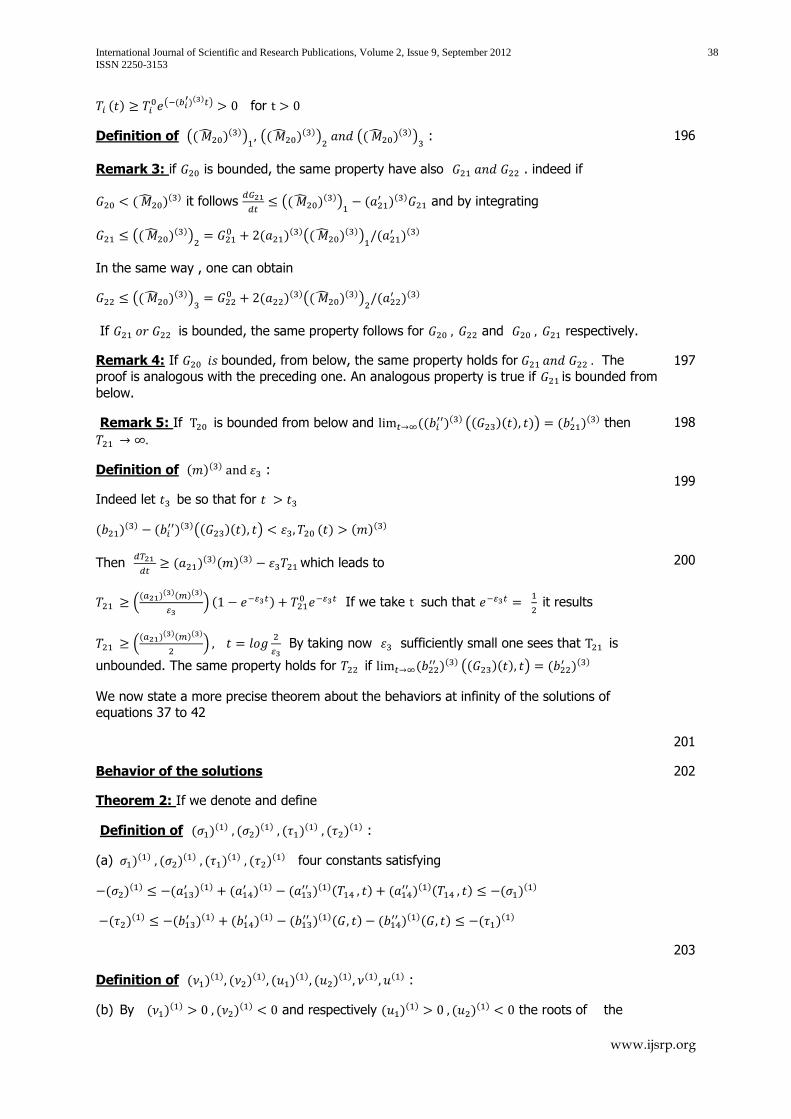
International Journal of Scientific and Research Publications, Volume 2, Issue 9, September 2012 38
ISSN 2250-3153
www.ijsrp.org
( ) ( (
)( ) ) for
Definition of (( )( ))
(( )
( )) (( )
( )) :
Remark 3: if is bounded, the same property have also . indeed if
( )( ) it follows
(( )
( )) (
)( ) and by integrating
(( )( ))
( )( )(( )
( )) (
)( )
In the same way , one can obtain
(( )( ))
( )( )(( )
( )) (
)( )
If is bounded, the same property follows for and respectively.
196
Remark 4: If bounded, from below, the same property holds for The
proof is analogous with the preceding one. An analogous property is true if is bounded from
below.
197
Remark 5: If is bounded from below and (( )( ) (( )( ) )) (
)( ) then
Definition of ( )( ) :
Indeed let be so that for
( )( ) (
)( )(( )( ) ) ( ) ( )( )
198
199
Then
( )
( )( )( ) which leads to
.( )
( )( )( )
/ ( )
If we take such that
it results
.( )
( )( )( )
/
By taking now sufficiently small one sees that is
unbounded. The same property holds for if ( )( ) (( )( ) ) (
)( )
We now state a more precise theorem about the behaviors at infinity of the solutions of
equations 37 to 42
200
201
Behavior of the solutions
Theorem 2: If we denote and define
Definition of ( )( ) ( )
( ) ( )( ) ( )
( ) :
(a) )( ) ( )
( ) ( )( ) ( )
( ) four constants satisfying
( )( ) (
)( ) ( )( ) (
)( )( ) ( )( )( ) ( )
( )
( )( ) (
)( ) ( )( ) (
)( )( ) ( )( )( ) ( )
( )
202
Definition of ( )( ) ( )
( ) ( )( ) ( )
( ) ( ) ( ) :
(b) By ( )( ) ( )
( ) and respectively ( )( ) ( )
( ) the roots of the
203
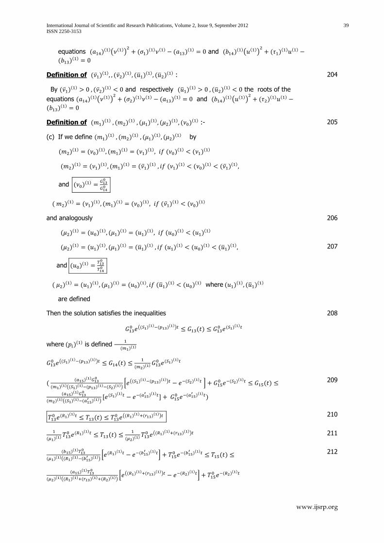
International Journal of Scientific and Research Publications, Volume 2, Issue 9, September 2012 39
ISSN 2250-3153
www.ijsrp.org
equations ( )( )( ( ))
( )
( ) ( ) ( )( ) and ( )
( )( ( )) ( )
( ) ( )
( )( )
Definition of ( )( ) ( )
( ) ( )( ) ( )
( ) :
By ( )( ) ( )
( ) and respectively ( )( ) ( )
( ) the roots of the
equations ( )( )( ( ))
( )
( ) ( ) ( )( ) and ( )
( )( ( )) ( )
( ) ( )
( )( )
204
Definition of ( )( ) ( )
( ) ( )( ) ( )
( ) ( )( ) :-
(c) If we define ( )( ) ( )
( ) ( )( ) ( )
( ) by
( )( ) ( )
( ) ( )( ) ( )
( ) ( )( ) ( )
( )
( )( ) ( )
( ) ( )( ) ( )
( ) ( )( ) ( )
( ) ( )( )
and ( )( )
( )( ) ( )
( ) ( )( ) ( )
( ) ( )( ) ( )
( )
205
and analogously
( )( ) ( )
( ) ( )( ) ( )
( ) ( )( ) ( )
( )
( )( ) ( )
( ) ( )( ) ( )
( ) ( )( ) ( )
( ) ( )( )
and ( )( )
( )( ) ( )
( ) ( )( ) ( )
( ) ( )( ) ( )
( ) where ( )( ) ( )
( )
are defined
206
207
Then the solution satisfies the inequalities
(( )
( ) ( )( )) ( )
( )( )
where ( )( ) is defined
( )( )
(( )
( ) ( )( )) ( )
( )( )
( )( )
208
( ( )
( )
( )( )(( )
( ) ( )( ) ( )
( ))0 (( )
( ) ( )( )) ( )
( ) 1 ( )
( ) ( )
( )( )
( )( )(( )
( ) ( )( ))
, ( )( ) (
)( ) - (
)( ) )
209
( )
( ) ( ) (( )
( ) ( )( )) 210
( )( )
( )( ) ( )
( )( )
(( )( ) ( )
( )) 211
( )( )
( )( )(( )
( ) ( )( ))
0 ( )( ) (
)( ) 1 (
)( ) ( )
( )( )
( )( )(( )
( ) ( )( ) ( )
( ))0 (( )
( ) ( )( )) ( )
( ) 1 ( )
( )
212

International Journal of Scientific and Research Publications, Volume 2, Issue 9, September 2012 40
ISSN 2250-3153
www.ijsrp.org
Definition of ( )( ) ( )
( ) ( )( ) ( )
( ):-
Where ( )( ) ( )
( )( )( ) (
)( )
( )( ) ( )
( ) ( )( )
( )( ) ( )
( )( )( ) (
)( )
( )( ) (
)( ) ( )( )
213
214
Behavior of the solutions
If we denote and define
215
Definition of ( )( ) ( )
( ) ( )( ) ( )
( ) :
(d) )( ) ( )
( ) ( )( ) ( )
( ) four constants satisfying
216
( )( ) (
)( ) ( )( ) (
)( )( ) ( )( )( ) ( )
( ) 217
( )( ) (
)( ) ( )( ) (
)( )(( ) ) ( )( )(( ) ) ( )
( ) 218
Definition of ( )( ) ( )
( ) ( )( ) ( )
( ) : 219
By ( )( ) ( )
( ) and respectively ( )( ) ( )
( ) the roots 220
(e) of the equations ( )( )( ( ))
( )
( ) ( ) ( )( ) 221
and ( )( )( ( ))
( )
( ) ( ) ( )( ) and 222
Definition of ( )( ) ( )
( ) ( )( ) ( )
( ) : 223
By ( )( ) ( )
( ) and respectively ( )( ) ( )
( ) the 224
roots of the equations ( )( )( ( ))
( )
( ) ( ) ( )( ) 225
and ( )( )( ( ))
( )
( ) ( ) ( )( ) 226
Definition of ( )( ) ( )
( ) ( )( ) ( )
( ) :- 227
(f) If we define ( )( ) ( )
( ) ( )( ) ( )
( ) by 228
( )( ) ( )
( ) ( )( ) ( )
( ) ( )( ) ( )
( ) 229
( )( ) ( )
( ) ( )( ) ( )
( ) ( )( ) ( )
( ) ( )( )
and ( )( )
230
( )( ) ( )
( ) ( )( ) ( )
( ) ( )( ) ( )
( ) 231
and analogously
( )( ) ( )
( ) ( )( ) ( )
( ) ( )( ) ( )
( )
232
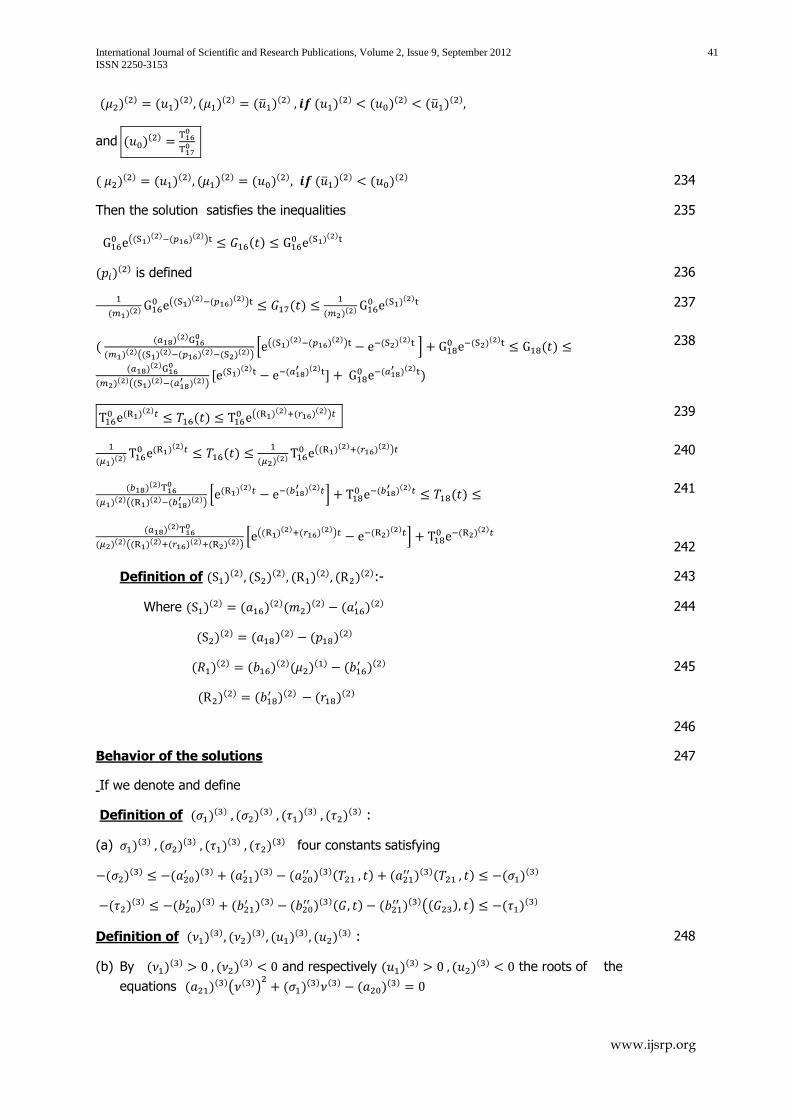
International Journal of Scientific and Research Publications, Volume 2, Issue 9, September 2012 41
ISSN 2250-3153
www.ijsrp.org
( )( ) ( )
( ) ( )( ) ( )
( ) ( )( ) ( )
( ) ( )( )
and ( )( )
( )( ) ( )
( ) ( )( ) ( )
( ) ( )( ) ( )
( ) 234
Then the solution satisfies the inequalities
(( )
( ) ( )( )) ( )
( )( )
235
( )( ) is defined 236
( )( )
(( )( ) ( )
( )) ( )
( )( )
( )( ) 237
( ( )
( )
( )( )(( )
( ) ( )( ) ( )
( ))0 (( )
( ) ( )( )) ( )
( ) 1 ( )
( ) ( )
( )( )
( )( )(( )
( ) ( )( ))
, ( )( ) (
)( ) - (
)( ) )
238
( )
( ) ( ) (( )
( ) ( )( )) 239
( )( )
( )( ) ( )
( )( )
(( )( ) ( )
( )) 240
( )( )
( )( )(( )
( ) ( )( ))
0 ( )( ) (
)( ) 1 (
)( ) ( )
( )( )
( )( )(( )
( ) ( )( ) ( )
( ))0 (( )
( ) ( )( )) ( )
( ) 1 ( )
( )
241
242
Definition of ( )( ) ( )
( ) ( )( ) ( )
( ):- 243
Where ( )( ) ( )
( )( )( ) (
)( )
( )( ) ( )
( ) ( )( )
244
( )( ) ( )
( )( )( ) (
)( )
( )( ) (
)( ) ( )( )
245
246
Behavior of the solutions
If we denote and define
Definition of ( )( ) ( )
( ) ( )( ) ( )
( ) :
(a) )( ) ( )
( ) ( )( ) ( )
( ) four constants satisfying
( )( ) (
)( ) ( )( ) (
)( )( ) ( )( )( ) ( )
( )
( )( ) (
)( ) ( )( ) (
)( )( ) ( )( )(( ) ) ( )
( )
247
Definition of ( )( ) ( )
( ) ( )( ) ( )
( ) :
(b) By ( )( ) ( )
( ) and respectively ( )( ) ( )
( ) the roots of the
equations ( )( )( ( ))
( )
( ) ( ) ( )( )
248

International Journal of Scientific and Research Publications, Volume 2, Issue 9, September 2012 42
ISSN 2250-3153
www.ijsrp.org
and ( )( )( ( ))
( )
( ) ( ) ( )( ) and
By ( )( ) ( )
( ) and respectively ( )( ) ( )
( ) the
roots of the equations ( )( )( ( ))
( )
( ) ( ) ( )( )
and ( )( )( ( ))
( )
( ) ( ) ( )( )
Definition of ( )( ) ( )
( ) ( )( ) ( )
( ) :-
(c) If we define ( )( ) ( )
( ) ( )( ) ( )
( ) by
( )( ) ( )
( ) ( )( ) ( )
( ) ( )( ) ( )
( )
( )( ) ( )
( ) ( )( ) ( )
( ) ( )( ) ( )
( ) ( )( )
and ( )( )
( )( ) ( )
( ) ( )( ) ( )
( ) ( )( ) ( )
( )
249
and analogously
( )( ) ( )
( ) ( )( ) ( )
( ) ( )( ) ( )
( )
( )( ) ( )
( ) ( )( ) ( )
( ) ( )( ) ( )
( ) ( )( ) and ( )
( )
( )( ) ( )
( ) ( )( ) ( )
( ) ( )( ) ( )
( )
Then the solution satisfies the inequalities
(( )
( ) ( )( )) ( )
( )( )
( )( ) is defined
250
251
( )( )
(( )( ) ( )
( )) ( )
( )( )
( )( ) 252
( ( )
( )
( )( )(( )
( ) ( )( ) ( )
( ))0 (( )
( ) ( )( )) ( )
( ) 1 ( )
( ) ( )
( )( )
( )( )(( )
( ) ( )( ))
, ( )( ) (
)( ) - (
)( ) )
253
( )
( ) ( ) (( )
( ) ( )( )) 254
( )( )
( )( ) ( )
( )( )
(( )( ) ( )
( )) 255
( )( )
( )( )(( )
( ) ( )( ))
0 ( )( ) (
)( ) 1 (
)( ) ( )
( )( )
( )( )(( )
( ) ( )( ) ( )
( ))0 (( )
( ) ( )( )) ( )
( ) 1 ( )
( )
256
Definition of ( )( ) ( )
( ) ( )( ) ( )
( ):-
Where ( )( ) ( )
( )( )( ) (
)( )
( )( ) ( )
( ) ( )( )
257

International Journal of Scientific and Research Publications, Volume 2, Issue 9, September 2012 43
ISSN 2250-3153
www.ijsrp.org
( )( ) ( )
( )( )( ) (
)( )
( )( ) (
)( ) ( )( )
258
FROM GLOBAL EQUATIONS WE OBTAIN:
( )
( )
( ) .( )( ) (
)( ) ( )( )( )/ (
)( )( ) ( ) ( )
( ) ( )
Definition of ( ) :- ( )
It follows
.( )( )( ( ))
( )
( ) ( ) ( )( )/
( )
.( )
( )( ( )) ( )
( ) ( ) ( )( )/
From which one obtains
Definition of ( )( ) ( )
( ) :-
(a) For ( )( )
( )
( ) ( )( )
( )( ) ( )
( ) ( )( )( )( )
0 ( )( ).( )( ) ( )( )/ 1
( )( ) 0 ( )( ).( )( ) ( )( )/ 1
, ( )( ) ( )
( ) ( )( )
( )( ) ( )
( )
( )( ) ( )( ) ( )
( )
259
260
In the same manner , we get
( )( ) ( )
( ) ( )( )( )( )
0 ( )( ).( )( ) ( )( )/ 1
( )( ) 0 ( )( ).( )( ) ( )( )/ 1
, ( )( ) ( )
( ) ( )( )
( )( ) ( )
( )
From which we deduce ( )( ) ( )( ) ( )
( )
(b) If ( )( ) ( )
( )
( )
( ) we find like in the previous case,
( )( )
( )( ) ( )( )( )
( ) 0 ( )( ).( )( ) ( )( )/ 1
( )( ) 0 ( )( ).( )( ) ( )( )/ 1
( )( )
( )
( ) ( )( )( )( )
0 ( )( ).( )( ) ( )( )/ 1
( )( ) 0 ( )( ).( )( ) ( )( )/ 1
( )( )
261
(c) If ( )( ) ( )
( ) ( )( )
, we obtain
262

International Journal of Scientific and Research Publications, Volume 2, Issue 9, September 2012 44
ISSN 2250-3153
www.ijsrp.org
( )( ) ( )( )
( )( ) ( )( )( )
( ) 0 ( )( ).( )( ) ( )( )/ 1
( )( ) 0 ( )( ).( )( ) ( )( )/ 1
( )( )
And so with the notation of the first part of condition (c) , we have
Definition of ( )( ) :-
( )( ) ( )( ) ( )
( ), ( )( ) ( )
( )
In a completely analogous way, we obtain
Definition of ( )( ) :-
( )( ) ( )( ) ( )
( ), ( )( ) ( )
( )
Now, using this result and replacing it in GLOBAL EQUATIONS we get easily the result stated in the theorem.
Particular case :
If ( )( ) (
)( ) ( )( ) ( )
( ) and in this case ( )( ) ( )
( ) if in addition
( )( ) ( )
( ) then ( )( ) ( )( ) and as a consequence ( ) ( )
( ) ( ) this also
defines ( )( ) for the special case
Analogously if ( )( ) (
)( ) ( )( ) ( )
( ) and then
( )( ) ( )
( )if in addition ( )( ) ( )
( ) then ( ) ( )( ) ( ) This is an important
consequence of the relation between ( )( ) and ( )
( ) and definition of ( )( )
263
: From GLOBAL EQUATIONS we obtain
( )
( )
( ) .( )( ) (
)( ) ( )( )( )/ (
)( )( ) ( ) ( )
( ) ( )
264
Definition of ( ) :- ( )
265
It follows
.( )( )( ( ))
( )
( ) ( ) ( )( )/
( )
.( )
( )( ( )) ( )
( ) ( ) ( )( )/
266
From which one obtains
Definition of ( )( ) ( )
( ) :-
(d) For ( )( )
( )
( ) ( )( )
( )( ) ( )
( ) ( )( )( )( )
0 ( )( ).( )( ) ( )( )/ 1
( )( ) 0 ( )( ).( )( ) ( )( )/ 1
, ( )( ) ( )
( ) ( )( )
( )( ) ( )
( )
( )( ) ( )( ) ( )
( )
267
In the same manner , we get 268

International Journal of Scientific and Research Publications, Volume 2, Issue 9, September 2012 45
ISSN 2250-3153
www.ijsrp.org
( )( ) ( )
( ) ( )( )( )( )
0 ( )( ).( )( ) ( )( )/ 1
( )( ) 0 ( )( ).( )( ) ( )( )/ 1
, ( )( ) ( )
( ) ( )( )
( )( ) ( )
( )
From which we deduce ( )( ) ( )( ) ( )
( ) 269
(e) If ( )( ) ( )
( )
( )
( ) we find like in the previous case,
( )( )
( )( ) ( )( )( )
( ) 0 ( )( ).( )( ) ( )( )/ 1
( )( ) 0 ( )( ).( )( ) ( )( )/ 1
( )( )
( )
( ) ( )( )( )( )
0 ( )( ).( )( ) ( )( )/ 1
( )( ) 0 ( )( ).( )( ) ( )( )/ 1
( )( )
270
(f) If ( )( ) ( )
( ) ( )( )
, we obtain
( )( ) ( )( )
( )( ) ( )( )( )
( ) 0 ( )( ).( )( ) ( )( )/ 1
( )( ) 0 ( )( ).( )( ) ( )( )/ 1
( )( )
And so with the notation of the first part of condition (c) , we have
271
Definition of ( )( ) :-
( )( ) ( )( ) ( )
( ), ( )( ) ( )
( )
272
In a completely analogous way, we obtain
Definition of ( )( ) :-
( )( ) ( )( ) ( )
( ), ( )( ) ( )
( )
273
274
Now, using this result and replacing it in CONCATENATED GLOBAL EQUATIONS we get easily the result stated in the theorem.
275
Particular case :
If ( )( ) (
)( ) ( )( ) ( )
( ) and in this case ( )( ) ( )
( ) if in addition
( )( ) ( )
( ) then ( )( ) ( )( ) and as a consequence ( ) ( )
( ) ( )
Analogously if ( )( ) (
)( ) ( )( ) ( )
( ) and then
( )( ) ( )
( )if in addition ( )( ) ( )
( ) then ( ) ( )( ) ( ) This is an important
consequence of the relation between ( )( ) and ( )
( )
276
277
FROM GLOBAL EQUATIONS WE OBTAIN:
( )
( )
( ) .( )( ) (
)( ) ( )( )( )/ (
)( )( ) ( ) ( )
( ) ( )
278
Definition of ( ) :- ( )
279

International Journal of Scientific and Research Publications, Volume 2, Issue 9, September 2012 46
ISSN 2250-3153
www.ijsrp.org
It follows
.( )( )( ( ))
( )
( ) ( ) ( )( )/
( )
.( )
( )( ( )) ( )
( ) ( ) ( )( )/
From which one obtains
(a) For ( )( )
( )
( ) ( )( )
( )( ) ( )
( ) ( )( )( )( )
0 ( )( ).( )( ) ( )( )/ 1
( )( ) 0 ( )( ).( )( ) ( )( )/ 1
, ( )( ) ( )
( ) ( )( )
( )( ) ( )
( )
( )( ) ( )( ) ( )
( )
280
In the same manner , we get
( )( ) ( )
( ) ( )( )( )( )
0 ( )( ).( )( ) ( )( )/ 1
( )( ) 0 ( )( ).( )( ) ( )( )/ 1
, ( )( ) ( )
( ) ( )( )
( )( ) ( )
( )
Definition of ( )( ) :-
From which we deduce ( )( ) ( )( ) ( )
( )
281
(b) If ( )( ) ( )
( )
( )
( ) we find like in the previous case,
( )( )
( )( ) ( )( )( )
( ) 0 ( )( ).( )( ) ( )( )/ 1
( )( ) 0 ( )( ).( )( ) ( )( )/ 1
( )( )
( )
( ) ( )( )( )( )
0 ( )( ).( )( ) ( )( )/ 1
( )( ) 0 ( )( ).( )( ) ( )( )/ 1
( )( )
282
283
(c) If ( )( ) ( )
( ) ( )( )
, we obtain
( )( ) ( )( )
( )( ) ( )( )( )
( ) 0 ( )( ).( )( ) ( )( )/ 1
( )( ) 0 ( )( ).( )( ) ( )( )/ 1
( )( )
And so with the notation of the first part of condition (c) , we have
Definition of ( )( ) :-
( )( ) ( )( ) ( )
( ), ( )( ) ( )
( )
In a completely analogous way, we obtain
Definition of ( )( ) :-
( )( ) ( )( ) ( )
( ), ( )( ) ( )
( )
Now, using this result and replacing it in GLOBAL EQUATIONS we get easily the result stated
in the theorem.
284

International Journal of Scientific and Research Publications, Volume 2, Issue 9, September 2012 47
ISSN 2250-3153
www.ijsrp.org
Particular case :
If ( )( ) (
)( ) ( )( ) ( )
( ) and in this case ( )( ) ( )
( ) if in addition
( )( ) ( )
( ) then ( )( ) ( )( ) and as a consequence ( ) ( )
( ) ( )
Analogously if ( )( ) (
)( ) ( )( ) ( )
( ) and then
( )( ) ( )
( )if in addition ( )( ) ( )
( ) then ( ) ( )( ) ( ) This is an important
consequence of the relation between ( )( ) and ( )
( )
285
We can prove the following
Theorem 3: If ( )( ) (
)( ) are independent on , and the conditions
( )( )(
)( ) ( )( )( )
( )
( )( )(
)( ) ( )( )( )
( ) ( )( )( )
( ) ( )( )( )
( ) ( )( )( )
( )
( )( )(
)( ) ( )( )( )
( ) ,
( )( )(
)( ) ( )( )( )
( ) ( )( )( )
( ) ( )( )( )
( ) ( )( )( )
( )
( )( ) ( )
( ) as defined by equation 25 are satisfied , then the system
If ( )( ) (
)( ) are independent on , and the conditions 286
( )( )(
)( ) ( )( )( )
( ) 287
( )( )(
)( ) ( )( )( )
( ) ( )( )( )
( ) ( )( )( )
( ) ( )( )( )
( ) 288
( )( )(
)( ) ( )( )( )
( ) , 289
( )( )(
)( ) ( )( )( )
( ) ( )( )( )
( ) ( )( )( )
( ) ( )( )( )
( )
( )( ) ( )
( ) as defined are satisfied , then the system
290
If ( )( ) (
)( ) are independent on , and the conditions
( )( )(
)( ) ( )( )( )
( )
( )( )(
)( ) ( )( )( )
( ) ( )( )( )
( ) ( )( )( )
( ) ( )( )( )
( )
( )( )(
)( ) ( )( )( )
( ) ,
( )( )(
)( ) ( )( )( )
( ) ( )( )( )
( ) ( )( )( )
( ) ( )( )( )
( )
( )( ) ( )
( ) as defined are satisfied , then the system
291
( )( ) [(
)( ) ( )( )( )] 292
( )( ) [(
)( ) ( )( )( )] 293
( )( ) [(
)( ) ( )( )( )] 294
( )( ) ,(
)( ) ( )( )( ) - 295
( )( ) ,(
)( ) ( )( )( ) - 296
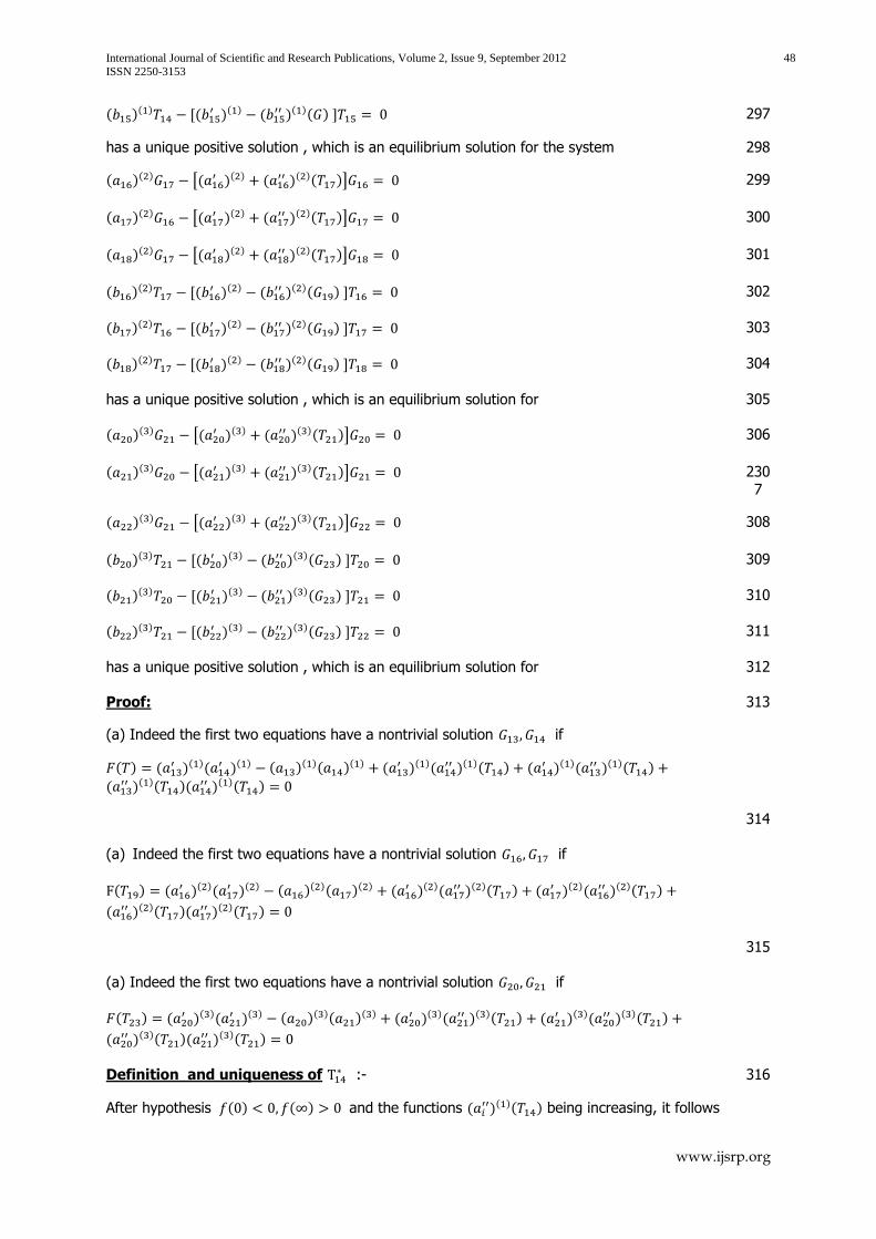
International Journal of Scientific and Research Publications, Volume 2, Issue 9, September 2012 48
ISSN 2250-3153
www.ijsrp.org
( )( ) ,(
)( ) ( )( )( ) - 297
has a unique positive solution , which is an equilibrium solution for the system 298
( )( ) [(
)( ) ( )( )( )] 299
( )( ) [(
)( ) ( )( )( )] 300
( )( ) [(
)( ) ( )( )( )] 301
( )( ) ,(
)( ) ( )( )( ) - 302
( )( ) ,(
)( ) ( )( )( ) - 303
( )( ) ,(
)( ) ( )( )( ) - 304
has a unique positive solution , which is an equilibrium solution for 305
( )( ) [(
)( ) ( )( )( )] 306
( )( ) [(
)( ) ( )( )( )] 230
7
( )( ) [(
)( ) ( )( )( )] 308
( )( ) ,(
)( ) ( )( )( ) - 309
( )( ) ,(
)( ) ( )( )( ) - 310
( )( ) ,(
)( ) ( )( )( ) - 311
has a unique positive solution , which is an equilibrium solution for 312
Proof:
(a) Indeed the first two equations have a nontrivial solution if
( ) ( )( )(
)( ) ( )( )( )
( ) ( )( )(
)( )( ) ( )( )(
)( )( )
( )( )( )(
)( )( )
313
(a) Indeed the first two equations have a nontrivial solution if
( ) ( )( )(
)( ) ( )( )( )
( ) ( )( )(
)( )( ) ( )( )(
)( )( )
( )( )( )(
)( )( )
314
(a) Indeed the first two equations have a nontrivial solution if
( ) ( )( )(
)( ) ( )( )( )
( ) ( )( )(
)( )( ) ( )( )(
)( )( )
( )( )( )(
)( )( )
315
Definition and uniqueness of :-
After hypothesis ( ) ( ) and the functions ( )( )( ) being increasing, it follows
316

International Journal of Scientific and Research Publications, Volume 2, Issue 9, September 2012 49
ISSN 2250-3153
www.ijsrp.org
that there exists a unique for which (
) . With this value , we obtain from the
three first equations
( )
( )
[( )( ) (
)( )( )]
, ( )
( )
[( )( ) (
)( )( )]
Definition and uniqueness of :-
After hypothesis ( ) ( ) and the functions ( )( )( ) being increasing, it follows
that there exists a unique for which (
) . With this value , we obtain from the
three first equations
317
( )
( )
[( )( ) (
)( )( )]
, ( )
( )
[( )( ) (
)( )( )]
318
Definition and uniqueness of :-
After hypothesis ( ) ( ) and the functions ( )( )( ) being increasing, it follows
that there exists a unique for which (
) . With this value , we obtain from the
three first equations
( )
( )
[( )( ) (
)( )( )]
, ( )
( )
[( )( ) (
)( )( )]
319
(b) By the same argument, the equations (SOLUTIONAL) admit solutions if
( ) ( )( )(
)( ) ( )( )( )
( )
[( )( )(
)( )( ) ( )( )(
)( )( )] ( )( )( )(
)( )( )
Where in ( ) must be replaced by their values. It is easy to see that is a
decreasing function in taking into account the hypothesis ( ) ( ) it follows
that there exists a unique such that ( )
320
(c) By the same argument, the equations (SOLUTIONAL) admit solutions if
( ) ( )( )(
)( ) ( )( )( )
( )
[( )( )(
)( )( ) ( )( )(
)( )( )] ( )( )( )(
)( )( )
321
Where in ( )( ) must be replaced by their values. It is easy to see that
is a decreasing function in taking into account the hypothesis ( ) ( ) it
follows that there exists a unique such that (( )
)
322
(d) By the same argument, the equations(SOLUTIONAL) admit solutions if
( ) ( )( )(
)( ) ( )( )( )
( )
[( )( )(
)( )( ) ( )( )(
)( )( )] ( )( )( )(
)( )( )
Where in ( ) must be replaced by their values from 96. It is easy to see
that is a decreasing function in taking into account the hypothesis ( ) ( )
it follows that there exists a unique such that (( )
)
323
Finally we obtain the unique solution
( ) ,
( ) and
324
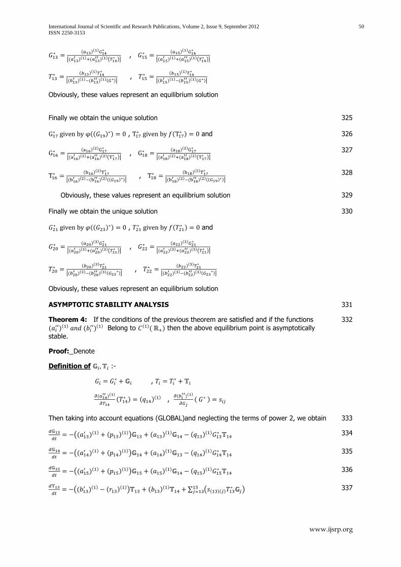
International Journal of Scientific and Research Publications, Volume 2, Issue 9, September 2012 50
ISSN 2250-3153
www.ijsrp.org
( )( )
[( )( ) (
)( )( )]
,
( )( )
[( )( ) (
)( )( )]
( )( )
[( )( ) (
)( )( )] ,
( )
( )
[( )( ) (
)( )( )]
Obviously, these values represent an equilibrium solution
Finally we obtain the unique solution 325
(( )
) , (
) and 326
( )( )
[( )( ) (
)( )( )]
,
( )( )
[( )( ) (
)( )( )]
327
( )( )
[( )( ) (
)( )(( ) )]
,
( )( )
[( )( ) (
)( )(( ) )]
328
Obviously, these values represent an equilibrium solution 329
Finally we obtain the unique solution
(( )
) , (
) and
( )( )
[( )( ) (
)( )( )]
,
( )( )
[( )( ) (
)( )( )]
( )( )
[( )( ) (
)( )( )]
,
( )( )
[( )( ) (
)( )( )]
Obviously, these values represent an equilibrium solution
330
ASYMPTOTIC STABILITY ANALYSIS
Theorem 4: If the conditions of the previous theorem are satisfied and if the functions
( )( ) (
)( ) Belong to ( )( ) then the above equilibrium point is asymptotically
stable.
Proof: Denote
Definition of :-
,
(
)( )
(
) ( )( ) ,
( )( )
( )
331
332
Then taking into account equations (GLOBAL)and neglecting the terms of power 2, we obtain 333
((
)( ) ( )( )) ( )
( ) ( )( )
334
((
)( ) ( )( )) ( )
( ) ( )( )
335
((
)( ) ( )( )) ( )
( ) ( )( )
336
((
)( ) ( )( )) ( )
( ) ∑ ( ( )( ) )
337

International Journal of Scientific and Research Publications, Volume 2, Issue 9, September 2012 51
ISSN 2250-3153
www.ijsrp.org
((
)( ) ( )( )) ( )
( ) ∑ ( ( )( ) )
338
((
)( ) ( )( )) ( )
( ) ∑ ( ( )( ) )
339
If the conditions of the previous theorem are satisfied and if the functions ( )( ) (
)( )
Belong to ( )( ) then the above equilibrium point is asymptotically stable
340
Denote
Definition of :-
341
,
342
( )( )
(
) ( )( ) ,
( )( )
( ( )
) 343
taking into account equations(GLOBAL) and neglecting the terms of power 2, we obtain 344
((
)( ) ( )( )) ( )
( ) ( )( )
345
((
)( ) ( )( )) ( )
( ) ( )( )
346
((
)( ) ( )( )) ( )
( ) ( )( )
347
((
)( ) ( )( )) ( )
( ) ∑ ( ( )( ) )
348
((
)( ) ( )( )) ( )
( ) ∑ ( ( )( ) )
349
((
)( ) ( )( )) ( )
( ) ∑ ( ( )( ) )
350
If the conditions of the previous theorem are satisfied and if the functions ( )( ) (
)( )
Belong to ( )( ) then the above equilibrium point is asymptotically sta
Denote
Definition of :-
,
(
)( )
(
) ( )( ) ,
( )( )
( ( )
)
351
352
Then taking into account equations (GLOBAL AND CONCATENATED) and neglecting the terms
of power 2, we obtain
353
((
)( ) ( )( )) ( )
( ) ( )( )
354
((
)( ) ( )( )) ( )
( ) ( )( )
355
((
)( ) ( )( )) ( )
( ) ( )( )
356
((
)( ) ( )( )) ( )
( ) ∑ ( ( )( ) )
357
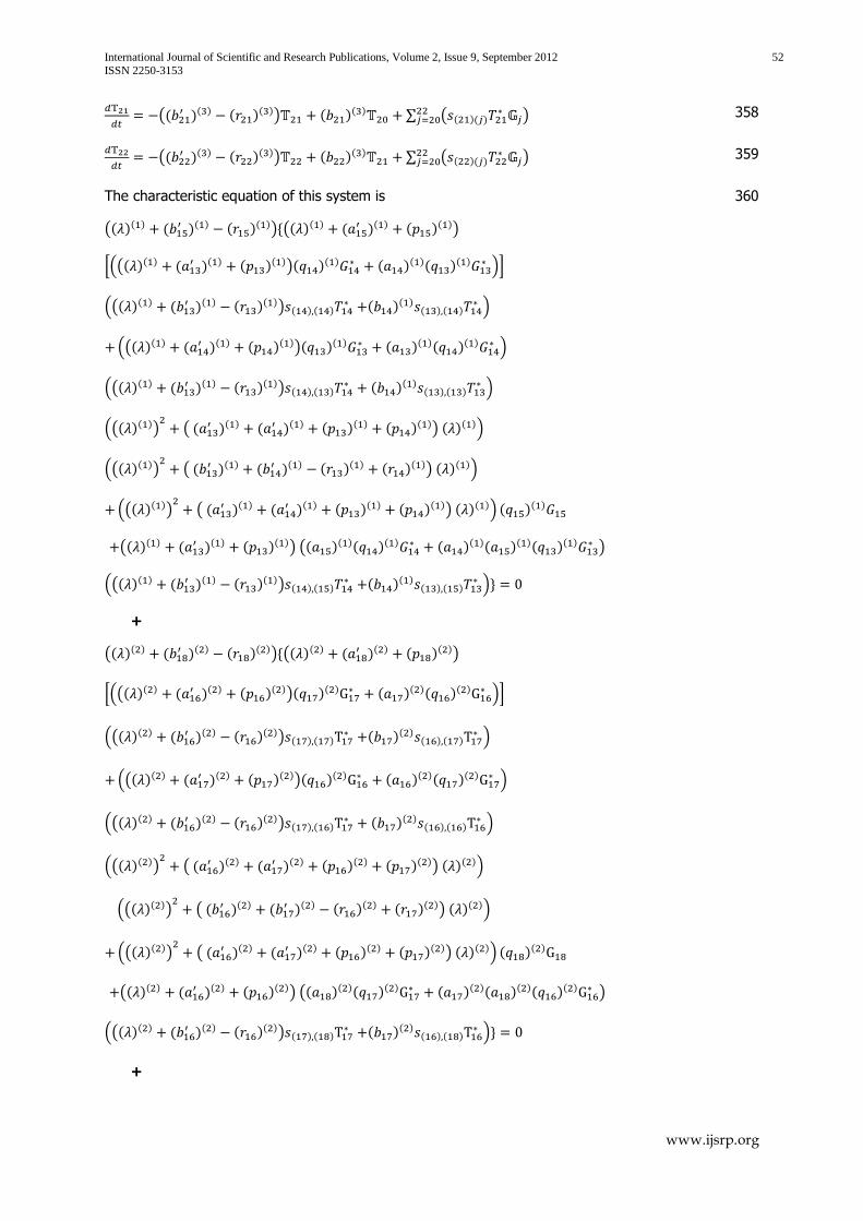
International Journal of Scientific and Research Publications, Volume 2, Issue 9, September 2012 52
ISSN 2250-3153
www.ijsrp.org
((
)( ) ( )( )) ( )
( ) ∑ ( ( )( ) )
358
((
)( ) ( )( )) ( )
( ) ∑ ( ( )( ) )
359
The characteristic equation of this system is
(( )( ) ( )( ) ( )
( ))*(( )( ) ( )( ) ( )
( ))
0.(( )( ) ( )( ) ( )
( ))( )( )
( )( )( )
( ) /1
.(( )( ) ( )( ) ( )
( )) ( ) ( ) ( )
( ) ( ) ( ) /
.(( )( ) ( )( ) ( )
( ))( )( )
( )( )( )
( ) /
.(( )( ) ( )( ) ( )
( )) ( ) ( ) ( )
( ) ( ) ( ) /
.(( )( )) ( (
)( ) ( )( ) ( )
( ) ( )( )) ( )( )/
.(( )( )) ( (
)( ) ( )( ) ( )
( ) ( )( )) ( )( )/
.(( )( )) ( (
)( ) ( )( ) ( )
( ) ( )( )) ( )( )/ ( )
( )
(( )( ) ( )( ) ( )
( )) (( )( )( )
( ) ( )
( )( )( )( )
( ) )
.(( )( ) ( )( ) ( )
( )) ( ) ( ) ( )
( ) ( ) ( ) /+
+
(( )( ) ( )( ) ( )
( ))*(( )( ) ( )( ) ( )
( ))
0.(( )( ) ( )( ) ( )
( ))( )( )
( )( )( )
( ) /1
.(( )( ) ( )( ) ( )
( )) ( ) ( ) ( )
( ) ( ) ( ) /
.(( )( ) ( )( ) ( )
( ))( )( )
( )( )( )
( ) /
.(( )( ) ( )( ) ( )
( )) ( ) ( ) ( )
( ) ( ) ( ) /
.(( )( )) ( (
)( ) ( )( ) ( )
( ) ( )( )) ( )( )/
.(( )( )) ( (
)( ) ( )( ) ( )
( ) ( )( )) ( )( )/
.(( )( )) ( (
)( ) ( )( ) ( )
( ) ( )( )) ( )( )/ ( )
( )
(( )( ) ( )( ) ( )
( )) (( )( )( )
( ) ( )
( )( )( )( )
( ) )
.(( )( ) ( )( ) ( )
( )) ( ) ( ) ( )
( ) ( ) ( ) /+
+
360
International Journal of Scientific and Research Publications, Volume 2, Issue 9, September 2012 53
ISSN 2250-3153
www.ijsrp.org
(( )( ) ( )( ) ( )
( ))*(( )( ) ( )( ) ( )
( ))
0.(( )( ) ( )( ) ( )
( ))( )( )
( )( )( )
( ) /1
.(( )( ) ( )( ) ( )
( )) ( ) ( ) ( )
( ) ( ) ( ) /
.(( )( ) ( )( ) ( )
( ))( )( )
( )( )( )
( ) /
.(( )( ) ( )( ) ( )
( )) ( ) ( ) ( )
( ) ( ) ( ) /
.(( )( )) ( (
)( ) ( )( ) ( )
( ) ( )( )) ( )( )/
.(( )( )) ( (
)( ) ( )( ) ( )
( ) ( )( )) ( )( )/
.(( )( )) ( (
)( ) ( )( ) ( )
( ) ( )( )) ( )( )/ ( )
( )
(( )( ) ( )( ) ( )
( )) (( )( )( )
( ) ( )
( )( )( )( )
( ) )
.(( )( ) ( )( ) ( )
( )) ( ) ( ) ( )
( ) ( ) ( ) /+
And as one sees, all the coefficients are positive. It follows that all the roots have negative real
part, and this proves the theorem.
Acknowledgments:
The introduction is a collection of information from various articles, Books, News
Paper reports, Home Pages Of authors, Journal Reviews, the internet including
Wikipedia. We acknowledge all authors who have contributed to the same. In the
eventuality of the fact that there has been any act of omission on the part of the
authors, We regret with great deal of compunction, contrition, and remorse. As
Newton said, it is only because erudite and eminent people allowed one to piggy
ride on their backs; probably an attempt has been made to look slightly further.
Once again, it is stated that the references are only illustrative and not
comprehensive
REFERENCES
1. Dr K N Prasanna Kumar, Prof B S Kiranagi, Prof C S Bagewadi - MEASUREMENT
DISTURBS EXPLANATION OF QUANTUM MECHANICAL STATES-A HIDDEN VARIABLE THEORY -
published at: "International Journal of Scientific and Research Publications, Volume 2, Issue 5,
May 2012 Edition".
2. DR K N PRASANNA KUMAR, PROF B S KIRANAGI and PROF C S BAGEWADI -CLASSIC 2
FLAVOUR COLOR SUPERCONDUCTIVITY AND ORDINARY NUCLEAR MATTER-A NEW PARADIGM STATEMENT - published at: "International Journal of Scientific and Research Publications, Volume 2, Issue 5, May 2012 Edition". 3. A HAIMOVICI: ―On the growth of a two species ecological system divided on age groups‖.
Tensor, Vol 37 (1982),Commemoration volume dedicated to Professor Akitsugu Kawaguchi on his 80th birthday
International Journal of Scientific and Research Publications, Volume 2, Issue 9, September 2012 54
ISSN 2250-3153
www.ijsrp.org
4. FRTJOF CAPRA: ―The web of life‖ Flamingo, Harper Collins See "Dissipative structures‖
pages 172-188
5. HEYLIGHEN F. (2001): "The Science of Self-organization and Adaptivity", in L. D. Kiel, (ed) . Knowledge Management, Organizational Intelligence and Learning, and Complexity,
in: The Encyclopedia of Life Support Systems ((EOLSS), (Eolss Publishers, Oxford) [http://www.eolss.net
6. MATSUI, T, H. Masunaga, S. M. Kreidenweis, R. A. Pielke Sr., W.-K. Tao, M. Chin, and Y. J
Kaufman (2006), ―Satellite-based assessment of marine low cloud variability associated with aerosol, atmospheric stability, and the diurnal cycle‖, J. Geophys. Res., 111,
D17204, doi:10.1029/2005JD006097
7. STEVENS, B, G. Feingold, W.R. Cotton and R.L. Walko, ―Elements of the microphysical structure of numerically simulated nonprecipitating stratocumulus‖ J. Atmos. Sci., 53, 980-
1006
8. FEINGOLD, G, Koren, I; Wang, HL; Xue, HW; Brewer, WA (2010), ―Precipitation-generated
oscillations in open cellular cloud fields‖ Nature, 466 (7308) 849-852, doi: 10.1038/nature09314, Published 12-Aug 2010
9. R WOOD ―The rate of loss of cloud droplets by coalescence in warm clouds‖ J.Geophys.
Res., 111, doi: 10.1029/2006JD007553, 2006
10. H. RUND, ―The Differential Geometry of Finsler Spaces‖, Grund. Math. Wiss. Springer-Verlag, Berlin, 1959
11. A. Dold, ―Lectures on Algebraic Topology‖, 1972, Springer-Verlag
12. S LEVIN ―Some Mathematical questions in Biology vii ,Lectures on Mathematics in life
sciences, vol 8‖ The American Mathematical society, Providence , Rhode island 1976
13.^ a b Einstein, Albert (1916). "The Foundation of the General Theory of
Relativity" (PDF). Annalen der
hysik. Bibcode 1916AnP...354...769E. DOI:10.1002/andp.19163540702.
14.^ Einstein, Albert (November 25, 1915). "Die Feldgleichungen der Gravitation". Sitzungsberichte der Preussischen Akademie der Wissenschaften zu Berlin: 844–
847. Retrieved 2006-09-12.(ENGLISH TRANSLATION)
15. ^ Carroll, Sean (2004). Spacetime and Geometry - An Introduction to General Relativity. pp. 151–15
17. ISBN0-8053-8732-3^ Weinberg, Steven (1993). Dreams of a Final Theory: the search for
the fundamental laws of nature. Vintage Press. p. 107, 233. ISBN 0-09-922391-18. ^ Gamow, George (April 28, 1970). My World Line : An Informal Autobiography. Viking Adult. ISBN 0-670-
50376-2. Retrieved 2007-03-14.
19^ Wahl, Nicolle (2005-11-22). "Was Einstein's 'biggest blunder' a stellar success?". Archived from the original on 2007-03-07. Retrieved 2007-03-14.
20.^ Turner, Michael S. (May, 2001). "Making Sense of the New Cosmology". Int.J.Mod.Phys.
A17S1 17: 180–196. ArXiv:astro-
ph/0202008. Bibcode 2002IJMPA..17S.180T.DOI:10.1142/S0217751X02013113.
21.^ Brown, Harvey (2005). Physical Relativity. Oxford University Press. p. 164. ISBN 978-0-
19-927583-0.
22.^ Trautman, Andrzej (1977). "Solutions of the Maxwell and Yang-Mills equations associated
with hopf fibrings". International Journal of Theoretical Physics 16 (9): 561–
International Journal of Scientific and Research Publications, Volume 2, Issue 9, September 2012 55
ISSN 2250-3153
www.ijsrp.org
565. Bibcode1977IJTP...16..561T. DOI:10.1007/BF01811088..
23.^ Stephani, Hans; D. Kramer, M. MacCallum, C. Hoenselaers and E. Herlt (2003). Exact
Solutions of Einstein's Field Equations. Cambridge University Press. ISBN 0-521-46136-7.
.
24.^ Beckner, W. (1975), "Inequalities in Fourier analysis", Annals of Mathematics 102 (6):
159–182, DOI:10.2307/1970980, JSTOR 1970980.
25.^ Bialynicki-Birula, I.; Mycielski, J. (1975), "Uncertainty Relations for Information Entropy in Wave Mechanics", Communications in Mathematical Physics 44 (2):
129, Bibcode1975CMaPh..44..129B, DOI:10.1007/BF01608825
26.^ Erhart, Jacqueline; Stephan Sponar, Georg Sulyok, Gerald Badurek, Masanao Ozawa, Yuji
Hasegawa (2012), "Experimental demonstration of a universally valid error-disturbance uncertainty relation in spin-measurements", Nature Physics 8: 185–
189,DOI:10.1038/nphys2194
27.^ American Physical Society online exhibit on the Uncertainty Principle.
28.^ Bohr, Niels (1958), Atomic Physics and Human Knowledge, New York: Wiley, p. 38(ENGLISH TRANSLATION)
29. ^ Tipler, Paul A.; Llewellyn, Ralph A. (1999), "5-5", Modern Physics (3rd ed.), W. H.
Freeman and Co., ISBN 1-57259-164-1
30.^ Feynman lectures on Physics, vol 3, 2-2
31. Gamow, G., The great physicists from Galileo to Einstein
First Author: 1Mr. K. N.Prasanna Kumar has three doctorates one each in Mathematics, Economics, Political Science. Thesis was based on Mathematical Modeling. He was recently awarded D.litt., for his work on ‗Mathematical Models in Political Science‘--- Department of studies in Mathematics, Kuvempu University, Shimoga, Karnataka, India Corresponding Author:[email protected]
Second Author: 2Prof. B.S Kiranagi is the Former Chairman of the Department of Studies in Mathematics, Manasa Gangotri and present Professor Emeritus of UGC in the Department. Professor Kiranagi has guided over 25 students and he has received many encomiums and laurels for his contribution to Co homology Groups and Mathematical Sciences. Known for his prolific writing, and one of the senior most Professors of the country, he has over 150 publications to his credit. A prolific writer and a prodigious thinker, he has to his credit several books on Lie Groups, Co Homology Groups, and other mathematical application topics, and excellent publication history.-- UGC Emeritus Professor (Department of studies in Mathematics), Manasagangotri, University of Mysore, Karnataka, India
Third Author: 3Prof. C.S. Bagewadi is the present Chairman of Department of Mathematics and
Department of Studies in Computer Science and has guided over 25 students. He has published

International Journal of Scientific and Research Publications, Volume 2, Issue 9, September 2012 56
ISSN 2250-3153
www.ijsrp.org
articles in both national and international journals. Professor Bagewadi specializes in Differential
Geometry and its wide-ranging ramifications. He has to his credit more than 159 research papers.
Several Books on Differential Geometry, Differential Equations are coauthored by him--- Chairman,
Department of studies in Mathematics and Computer science, Jnanasahyadri Kuvempu university,
Shankarghatta, Shimoga district, Karnataka, India


![Superconducting quantum bits...are canonically conjugate, as expressed by the commutator bracket [δ, Q] = i2e.The fact that δ and Q are subject to Heisenberg’s uncertainty principle](https://img.pdfslide.net/doc/110x75/5f80ec7baa4220151344eb0b/superconducting-quantum-bits-are-canonically-conjugate-as-expressed-by-the.jpg)