Embed Size (px)
Citation preview

UNIVERSITY OF NAIROBI
FACULTY OF ENGINEERING
DEPARTMENT OF ELECTRICAL AND INFORMATION ENGINEERING
SOLAR TRACKER FOR SOLAR PANEL
PROJECT INDEX: PRJ 031
BY
OLOKA REAGAN OTIENO
F17/2381/2009
SUPERVISOR: MR. S.A. Ahmed
EXAMINER: Professor Elijah Mwangi
Project report submitted in partial fulfillment of the requirement for the award for
the degree of
Bachelor of Science in ELECTRICAL AND ELECTRONICS ENGINEERING of the
University of Nairobi 2015
Submitted on: 24THApril, 2015

ii
DECLARATION OF ORIGINALITY
FACULTY/ SCHOOL/ INSTITUTE: Engineering
DEPARTMENT: Electrical and Information Engineering
COURSE NAME: Bachelor of Science in Electrical & Electronics Engineering
NAME OF STUDENT: Oloka Reagan Otieno
REGISTRATION NUMBER: F17/2381/2009
COLLEGE: Architecture & Engineering
WORK: SOLAR TRACKER FOR SOLAR PANEL
1) I understand what plagiarism is and I am aware of the university policy in this regard.
2) I declare that this final year project report is my original work and has not been
submitted elsewhere for examination, award of a degree or publication. Where other
people’s work or my own work has been used, this has properly been acknowledged and
referenced in accordance with the University of Nairobi’s requirements.
3) I have not sought or used the services of any professional agencies to produce this work.
4) I have not allowed, and shall not allow anyone to copy my work with the intention of
passing it off as his/her own work.
5) I understand that any false claim in respect of this work shall result in disciplinary
action, in accordance with University anti-plagiarism policy.
Signature:……………………… Date: ………………………
Approved by:
Supervisor: Mr. S. A. Ahmed
Signature:……………………… Date…………………………

iiiiiii
DEDICATIONTo my family for their support during my university education, particularly my Dad and sister
Linda Oloka for always being available for me and their unwavering support.
ivivi
ACKNOWLEDGEMENTI would like to express my gratitude to Mr. S.A. Ahmed, who was my supervisor, for his
constant guidance in the implementation of this project. I must particularly thank him for his
commitment and unrelenting effort to see me do all the assignments appertaining to this project
and finally I can say I am done. He was always available for consultation and ensured there
was no laxity in the implementation of the project. I particularly thank him for his insight, his
advice and help towards the overall success of this project. Without his encouragement, I am
not sure if the project would have been implemented as successfully as is the case.
Mr. Wangai of the mechanical workshop laboratory was very resourceful when it came
to building the mechanical structure and working on the PCB. I would also like to extend my
gratitude towards the examiner, Prof. Mwangi for taking his time to go through this project
documentation and also handling the presentation of the project.
Finally, I would also like to thank my friends and classmates with whom we spent
sleepless nights at times when trying to get some concepts right. My classmate Edkevin Chege
was one such person. My good friend Timothy Ndung’u Kyalo was very instrumental in
helping with the software part for which I was not too well conversant. Finally, I was able to
come up with a working project. Guys, that moral support and psyche could not have come at
a better time and for a better cause. I also thank my brother George Bush who was
instrumental when it came to designing the body of the project that was to hold the panel.
Above everything else, I thank the Lord for seeing me thus far with all this work. His guidance
is something I could not do without.

vv
TABLE OF CONTENTS
DECLARATION OF ORIGINALITY.................................................................................... ii
DEDICATION ........................................................................................................................ iii
ACKNOWLEDGEMENT ...................................................................................................... iv
LIST OF TABLES ................................................................................................................ viii
LIST OF FIGURES ................................................................................................................ ix
ABBREVIATIONS AND ACRONYMS ..................................................................................x
ABSTRACT............................................................................................................................. xi
CHAPTER ONE: INTRODUCTION ......................................................................................1
1.1 General background ..............................................................................................................1
1.2 Problem statement .................................................................................................................2
1.3 Project justification ...............................................................................................................2
1.4 Objectives .............................................................................................................................3
1.5 Scope of the project ...............................................................................................................3
1.6 Methodology .........................................................................................................................4
CHAPTER TWO LITERATURE REVIEW ...........................................................................5
2.1 Introduction...........................................................................................................................5
2.2 The Earth: Rotation and Revolution......................................................................................6
2.3 Solar Irradiation: Sunlight and the Solar Constant .................................................................7
2.4 Sunlight.................................................................................................................................8
2.4.1 Elevation angle ...............................................................................................................9
2.4.2 Zenith angle ....................................................................................................................9
2.4.3 Azimuth angle...............................................................................................................10
2.5 Types of solar trackers and tracking technologies ................................................................10

vivi
2.5.1 Active tracker ...............................................................................................................10

viiv
2.5.2 Passive solar tracking ....................................................................................................10
2.5.3 Chronological solar tracking .........................................................................................10
2.5.4 Single axis trackers .......................................................................................................11
2.5.5 Dual axis trackers..........................................................................................................11
2.6 Fixed and tracking collectors ...............................................................................................11
2.6.1 Fixed collectors.............................................................................................................11
2.6.2 CASE I: The Fixed Collector ........................................................................................13
2.6.3 Tracking collectors: Improvement of efficiency ............................................................13
2.6.4 CASE II: The Tracking Collector..................................................................................13
2.7 Effect of light intensity ........................................................................................................14
2.8 Efficiency of solar panels ....................................................................................................14
2.9 Benefits and demerits of solar energy ..................................................................................15
2.9.1 Benefits ........................................................................................................................15
2.9.2 Disadvantages of solar power........................................................................................15
CHAPTER THREE : DESIGN AND IMPLEMENTATION ...............................................17
3.1 Light Sensor Theory and Circuit of Sensor Used .................................................................17
3.2 Light Dependent Resistor Theory ........................................................................................17
3.2.1 The concept of using two LDRs........................................................................................18
3.3 Light sensor design..............................................................................................................18
3.4 Servo motor.........................................................................................................................20
3.4.1 Components of the servo motor.....................................................................................20
3.4.2 How the servo is controlled ...........................................................................................21
3.4.3 Advantages and disadvantages of servo motors .............................................................22
3.5 Crystal.................................................................................................................................22
3.6 Voltage regulation ...............................................................................................................23

vii
3.7 Microcontroller ...................................................................................................................25
3.7.1 ATmega328P ................................................................................................................26
3.8 The design tool....................................................................................................................29
Arduino IDE .............................................................................................................................29
3.9 Algorithm for Motor Control ...............................................................................................31
CHAPTER 4: RESULTS, SIMULATIONS AND ANALYSIS .............................................33
4.1 Results ................................................................................................................................33
4.2 Analysis ..............................................................................................................................37
CHAPTER FIVE: DISCUSSION, CONCLUSION AND RECOMMENDATIONS FOR
FURTHER WORK .................................................................................................................40
5.1 Discussion ...........................................................................................................................40
5.2 Conclusion ..........................................................................................................................41
5.3 Recommendations for further work .....................................................................................41
REFERENCES........................................................................................................................42
APPENDIXES .........................................................................................................................43
Appendix One: Code used in the microcontroller .....................................................................43
Appendix Two: Code for obtaining the results from the LDRs ..................................................46
Appendix Three: Code for obtaining the stored values of readings from the LDRs in Volts .......49
Appendix Four: Screenshot of some of the readings obtained ....................................................50

viiiviiiv
LIST OF TABLESTable 2.1: Range of the brightness of sunlight (lux).....................................................................9
Table 3.1 Photocell Resistance Testing Data .............................................................................19
Table 3.2: Pin Description ........................................................................................................24
Table 3.3 Pins and their functions..............................................................................................28
Table 4.1: Results for cloudy Morning and Sunny Afternoon for 6th and 7th April 2015 ............34
Table 4.2: LDR outputs for bright sunny day on 2nd April 2015 ................................................35
Table 4.3: Results for LDR outputs for a cloudy day on 12th April 2015 ....................................36

ixix
LIST OF FIGURESFigure 2.1: Solar Cell .................................................................................................................5
Figure 2.2: Earth’s rotation..........................................................................................................6
Figure 2.3: Revolution and rotation……………………………………………………………...19
Figure 2.4: angle of elevation and zenith angle ............................................................................9
Figure 2.5: Sun path diagram for Nairobi ................................................................................12
Figure 3.1: LDR construction ....................................................................................................17
Figure 3.2: use of two LDRs .....................................................................................................18
Figure 3.3: The input circuit that employs a voltage divider. .....................................................19
Figure 3.4: servo motor inside features ......................................................................................20
Figure 3.5: variable pulse width control servo position .............................................................21
Figure 3.6 circuit diagram of a crystal ......................................................................................23
Figure 3.7: Voltage Regulator Circuit LM7805 ........................................................................24
Figure 3.8: the LM7805 pin diagram ........................................................................................24
Figure 3.9: Microcontroller Architecture ..................................................................................26
Figure 3.10: Atmega 328P........................................................................................................27
Figure 3.11: A Simplified Flow Chart of the Assembly .............................................................30
Figure3.12: Hardware schematic diagram.................................................................................32
Figure4.1: Graph of results obtained on 6th and 7th April ...........................................................35
Figure 4.2: Graph for bright sunny day of 2nd April 2015 ..........................................................36
Figure 4.3: Graph of LDR outputs for a cloudy day on 12th April 2015.....................................37

xx
ABBREVIATIONS AND ACRONYMS
ADC Analog to Digital Converter
EEPROM Electrical Erasable programmable Read Only Memory
D Diode
DC Direct current
GND Ground
I Current
I/O Input/ Output
IDE Integrated Development Environment
LDR Light Dependent Resistor
LED Light Emitting Diode
LUX Luminous Flux
LED Light Emitting Diode
MAX Maximum
MCU Microcontroller
MIN Minimum
VCC Supply voltage
UV Ultra Violet Light
PCB Printed Circuit Board
PV Photovoltaic panels
R Resistor
GaAs Gallium Arsenide
MPPT Maximum Power Point Tracking
CMOS Complementary Metal–Oxide–Semiconductor
RISC Reduced Instruction Set Computing
IDE Integrated Development
Environment PWM Pulse Width

xixi
Modulation
xiix
ABSTRACTSolar energy is fast becoming a very important means of renewable energy resource. With solar
tracking, it will become possible to generate more energy since the solar panel can maintain a
perpendicular profile to the rays of the sun. Even though the initial cost of setting up the
tracking system is considerably high, there are cheaper options that have been proposed over
time. This project discuses the design and construction of a prototype for solar tracking system
that has a single axis of freedom. Light Dependent Resistors (LDRs) are used for sunlight
detection.
The control circuit is based on an ATMega328P microcontroller. It was programmed to detect
sunlight via the LDRs before actuating the servo to position the solar panel. The solar panel is
positioned where it is able to receive maximum light. As compared to other motors, the servo
motors are able to maintain their torque at high speed. They are also more efficient
with efficiencies in the range of 80-90%. Servos can supply roughly twice their rated torque for
short periods. They are also quiet and do not vibrate or suffer resonance issues. Performance
and characteristics of solar panels are analyzed experimentally.
Silicon solar cells produced an efficiency of 20% for the first time in 1985. Whereas there has
been a steady increase in the efficiency of solar panels, the level is still not at its best.
Most panels still operate at less than 40%. As a result, most people are forced to either
purchase a number of panels to meet their energy demands or purchase single systems with
large outputs. There are types of solar cells with relatively higher efficiencies but they tend to
be very costly.
One of the ways to increase the efficiency of solar panels while reducing costs is to use
tracking. Through tracking, there will be increased exposure of the panel to the sun,
making it have increased power output. The trackers can either be dual or single axis trackers.
Dual trackers are more efficient because they track sunlight from both axes.
A single tracking system was used. It is cheaper, less complex and still achieves the required
efficiency. In terms of costs and whether or not the system is supposed to be implemented by
those that use solar panels, the system is viable. The increase in power is considerable and
therefore worth the small increase in cost. Maintenance costs are not likely to be high.

1
CHAPTER ONE: INTRODUCTION
1.1 General backgroundSolar energy is clean and available in abundance. Solar technologies use the sun for provision
of heat, light and electricity. These are for industrial and domestic applications. With the
alarming rate of depletion of depletion of major conventional energy sources like petroleum,
coal and natural gas, coupled with environmental caused by the process of harnessing
these energy sources, it has become an urgent necessity to invest in renewable energy sources
that can power the future sufficiently. The energy potential of the sun is immense.
Despite the unlimited resource however, harvesting it presents a challenge because of the
limited efficiency of the array cells.
The best efficiency of the majority of commercially available solar cells ranges between 10 and
20 percent. This shows that there is still room for improvement. This project seeks to identify a
way of improving efficiency of solar panels. Solar tracking is used. The tracking mechanism
moves and positions the solar array such that it is positioned for maximum power output.
Other ways include identifying sources of losses and finding ways to mitigate them.
When it comes to the development of any nation, energy is the main driving factor. There is an
enormous quantity of energy that gets extracted, distributed, converted and consumed
every single day in the global society. Fossil fuels account for around 85 percent of energy that
is produced. Fossil fuel resources are limited and using them is known to cause global warming
because of emission of greenhouse gases. There is a growing need for energy from such
sources as solar, wind, ocean tidal waves and geothermal for the provision of sustainable and
power.
Solar panels directly convert radiation from the sun into electrical energy. The panels are
mainly manufactured from semiconductor materials, notably silicon. Their efficiency is 24.5%
on the higher side. Three ways of increasing the efficiency of the solar panels are through
increase of cell efficiency, maximizing the power output and the use of a tracking system.
Maximum power point tracking (MPPT) is the process of maximizing the power output from
the solar panel by keeping its operation on the knee point of P-V characteristics. MPPT

2
technology will only offer maximum power which can be received from stationary arrays of
solar panels at

2
any given time. The technology cannot however increase generation of power when the sun
is not aligned with the system.
Solar tracking is a system that is mechanized to track the position of the sun to increase power
output by between 30% and 60% than systems that are stationary. It is a more cost effective
solution than the purchase of solar panels.
There are various types of trackers that can be used for increase in the amount of energy that
can be obtained by solar panels. Dual axis trackers are among the most efficient, though this
comes with increased complexity. Dual trackers track sunlight from box axes. They are the best
option for places where the position of the sun keeps changing during the year at different
seasons. Single axis trackers are a better option for places around the equator where there is no
significant change in the apparent position of the sun.
The level to which the efficiency is improved will depend on the efficiency of the
tracking system and the weather. Very efficient trackers will offer more efficiency because
they are able to track the sun with more precision. There will be bigger increase in efficiency
in cases where the weather is sunny and thus favorable for the tracking system [1].
1.2 Problem statementA solar tracker is used in various systems for the improvement of harnessing of solar radiation.
The problem that is posed is the implementation of a system which is capable of enhancing
production of power by 30-40%. The control circuit is implemented by the microcontroller.
The control circuit then positions the motor that is used to orient the solar panel optimally.
1.3 Project justificationThe project was undertaken to ensure the rays of the sun are falling perpendicularly on the
solar panel to give it maximum solar energy. This is harnessed into electrical power. Maximum
energy is obtained between 1200hrs and 1400hrs, with the peak being around midday. At this
time, the sun is directly overhead. At the same time, the least energy will be required to move
the panel, something that will further increase efficiency of the system. The project was
designed to address the challenge of low power, accurate and economical microcontroller based
tracking system which is implemented within the allocated time and with the available
3
resources. It is

4
supposed to track the sun’s movement in the sky. In order to save power, it is supposed to
sleep during the night by getting back into an horizontal position. There is implementation of
an algorithm that solves the motor control that is then written into C- program on Arduino IDE.
1.4 ObjectivesThe project was carried out to satisfy two main objectives:
Design a system that tracks the solar UV light for solar panels.
Prove that the tracking indeed increases the efficiency considerably. The range
of increase in efficiency is expected to be between 30 and 40 percent.
1.5 Scope of the projectThe solar project was implemented using a servo motor. The choice was informed by the
fact that the motor is fast, can sustain high torque, has precise rotation within limited angle and
does not produce any noise. There is the embedded software section where the Atmega 328P is
programmed using the C language before the chip removed from the Arduino board.
The Arduino IDE was used for the coding. It is then used as a standalone unit on a PCB during
fabrication and display. The design is limited to Single Axis tracking because the use of a
dual
axis tracking system would not add much value. Nairobi has coordinates of 1.2833⁰S,
36.8167⁰Eand therefore the position of the sun will not vary in a significant way during the year. In the
tropics, the sun position varies considerably during certain seasons. There is the design of
an input stage that facilitates conversion of light into a voltage by the light dependent resistors,
LDRs. There is comparison of the two voltages, then the microcontroller uses the difference
as the error. The servo motor uses this error to rotate through a corresponding angle for
the adjustment of the position of the solar panel until such a time that the voltage outputs
in the LDRs are equal.
The difference between the voltages of the LDRs is gotten as analog readings. The difference is
transmitted to the servo motor and it thus moves to ensure the two LDRs are an equal
inclination. This means they will be receiving the same amount of light. The procedure
is repeated throughout the day.

5
1.6 MethodologyThe circuit of the solar tracker system is divided into three sections. There is the input stage
that is composed of sensors and potentiometers, a program in embedded software in the
microcontroller and lastly the driving circuit that has the servo motor. The input stage has two
LDRs that are so arranged to form a voltage divider circuit. A C program loaded into the
Atmega
328P forms the embedded software. There is a metallic frame that houses the components. The
three stages are designed independently before being joined into one system. This approach,
similar to stepwise refinement in modular programming, has been employed as it ensures an
accurate and logical approach which is straight forward and easy to understand. This also
ensures that if there are any errors, they are independently considered and corrected.
Project report organization
The project is divided into 5 chapters;
Chapter 1: This is the introduction to the project report that describes the justification for
doing the project. The objectives, methodology and scope of the work are also described.
Chapter 2: This has the literature review that is based on the background of the problem. The
chapter also includes material studied and which is pertinent to the study. There is a brief
review of methods used for tracking and how tracking the apparent movement of the sun
increases efficiency of solar panels.
Chapter 3: The chapter involves the design and implementation of the project.
Chapter 4: It involves design of the system, simulations and implementation.
Chapter 5: This chapter has the discussion, conclusion and recommendations for further work
with regard to this project.

6
CHAPTER 2: LITERATURE REVIEW
2.1 IntroductionA solar tracker is a device used for orienting a photovoltaic array solar panel or for
concentrating solar reflector or lens toward the sun. The position of the sun in the sky is varied
both with seasons and time of day as the sun moves across the sky. Solar powered equipment
work best when they are pointed at the sun. Therefore, a solar tracker increases how
efficient such equipment are over any fixed position at the cost of additional complexity to
the system. There are different types of trackers.
Extraction of usable electricity from the sun became possible with the discovery of the
photoelectric mechanism and subsequent development of the solar cell. The solar cell is
a semiconductor material which converts visible light into direct current. Through the use of
solar arrays, a series of solar cells electrically connected, there is generation of a DC voltage
that can be used on a load. There is an increased use of solar arrays as their efficiencies
become higher. They are especially popular in remote areas where there is no connection to the
grid.
Photovoltaic energy is that which is obtained from the sun. A photovoltaic cell,
commonly known as a solar cell, is the technology used for conversion of solar directly
into electrical power. The photovoltaic cell is a non mechanical device made of silicon alloy.
Figure 2.1: Solar Cell

7
The photovoltaic cell is the basic building block of a photovoltaic system. The individual
cells can vary from 0.5 inches to 4 inches across. One cell can however produce only 1 or 2
watts that is not enough for most appliances. Performance of a photovoltaic array depends on
sunlight. Climatic conditions like clouds and fog significantly affect the amount of solar
energy that is received by the array and therefore its performance. Most of the PV modules are
between 10 and
20 percent efficient [4].
2.2 The Earth: Rotation and RevolutionThe earth is a planet of the sun and revolves around it. Besides that, it also rotates around its
own axis. There are thus two motions of the earth, rotation and revolution. The earth rotates
on its axis from west to east. The axis of the earth is an imaginary line that passes through the
northern and southern poles of the earth. The earth completes its rotation in 24 hours. This
motion is responsible for occurrence of day and night. The solar day is a time period of 24
hours and the duration of a sidereal is 23 hours and 56 minutes. The difference of 4 minutes is
because of the fact that the earth’s position keeps changing with reference to the sun.
Figure 2.2: Earth’s rotation

8
The movement of the earth round the sun is known as revolution. It also happens from west to
east and takes a period of 365 days. The orbit of the earth is elliptical. Because of this
the distance between the earth and the sun keeps changing. The apparent annual track of the sun
via the fixed stars in the celestial sphere is known as the ecliptic. The earth’s axis makes an
angle of
66.5 degrees to the ecliptic plane. Because of this, the earth attains four critical positions with
reference to the sun [7].
Figure 2.3: Revolution and rotation
2.3 Solar Irradiation: Sunlight and the Solar ConstantThe sun delivers energy by means of electromagnetic radiation. There is solar fusion that
results from the intense temperature and pressure at the core of the sun. Protons get converted
into helium atoms at 600 million tons per second. Because the output of the process has lower
energy than the protons which began, fusion gives rise to lots of energy in form of gamma rays
that are absorbed by particles in the sun and re-emitted.
The total power of the sun can be estimated by the law of Stefan and Boltzmann.
P=4πr2 σϵT4 W [1]
T is the temperature that is about 5800K, r is the radius of the sun which is 695800 km and σ is
the Boltzmann constant which is 1.3806488 × 10⁻²³ m2 kg s-2 K-1. The emissivity of the surface is
denoted by ϵ. Because of Einstein’s famous law E=mc2 about millions of tons of matter
9
are
converted to energy each second. The solar energy that is irradiated to the earth is 5.1024
Joules
per year. This is 10000 times the present worldwide energy consumption per year.
Solar radiation from the sun is received in three ways: direct, diffuse and
reflected.

10
Direct radiation: is also referred to as beam radiation and is the solar radiation which travels on
a straight line from the sun to the surface of the earth.
Diffuse radiation: is the description of the sunlight which has been scattered by particles and
molecules in the atmosphere but still manage to reach the earth’s surface. Diffuse radiation
has no definite direction, unlike direct versions.
Reflected radiation: describes sunlight which has been reflected off from non-atmospheric
surfaces like the ground [8].
2.4 Sunlight
Photometry enables us to determine the amount of light given off by the Sun in terms of
brightness perceived by the human eye. In photometry, a luminosity function is used for the
radiant power at each wavelength to give a different weight to a particular wavelength
that models human brightness sensitivity. Photometric measurements began as early as the end
of the
18th century resulting in many different units of measurement, some of which cannot even be
converted owing to the relative meaning of brightness. However, the luminous flux (or lux) is
commonly used and is the measure of the perceived power of light. Its unit, the lumen, is
concisely defined as the luminous flux of light produced by a light source that emits one
candela of luminous intensity over a solid angle of one steradian. The candela is the SI unit of
luminous intensity and it is the power emitted by a light source in a particular direction,
weighted by a luminosity function whereas a steradian is the SI unit for a solid angle; the
two-dimensional angle in three-dimensional space that an object subtends at a point.
One lux is equivalent to one lumen per square metre;1 lx = 1lm ∙ m �ିଶ = 1 cd ∙ sr ∙ m �ି ଶ (1)
i.e. a flux of 10 lumen, concentrated over an area of 1 square metre, lights up that area with
illuninance of 10 lux [1].

11
Sunlight ranges between 400 lux and approximately 130000 lux, as summarized in the table
below.
12
Table 2.1: Range of the brightness of sunlight (lux)Luminous flux (lux)
Time of day
Sunrise or sunset on a clear day 400
Overcast day 1000
Full day (not direct sun) 10000 – 25000
Direct sunlight 32000 – 130000
2.4.1 Elevation angleThe elevation angle is used interchangeably with altitude angle and is the angular height of
the sun in the sky measured from the horizontal. Both altitude and elevation are used for
description of the height in meters above the sea level. The elevation is 0 degrees at sunrise
and 90 degrees when the sun is directly overhead. The angle of elevation varies throughout the
day and also depends on latitude of the particular location and the day of the year.
2.4.2 Zenith angleThis is the angle between the sun and the vertical. It is similar to the angle of elevation but is
measured from the vertical rather than from the horizontal. Therefore, the zenith angle = 90
degrees – elevation angle [8].
Figure 2.4: angle of elevation and zenith angle

1010
2.4.3 Azimuth angleThis is the compass direction from which the sunlight is coming. At solar noon, the sun
is directly south in the northern hemisphere and directly north in the southern hemisphere. The
azimuth angle varies throughout the day. At the equinoxes, the sun rises directly east and sets
directly west regardless of the latitude. Therefore, the azimuth angles are 90 degrees at sunrise
and 270 degrees at sunset [8].
2.5 Types of solar trackers and tracking technologiesThere are various categories of modern solar tracking technologies;
2.5.1 Active trackerActive trackers make use of motors and gear trains for direction of the tracker as commanded
by the controller responding to the solar direction. The position of the sun is monitored
throughout the day. When the tracker is subjected to darkness, it either sleeps or stops
depending on the design. This is done using sensors that are sensitive to light such as LDRs.
Their voltage output is put into a microcontroller that then drives actuators to adjust the position
of the solar panel [7].
2.5.2 Passive solar trackingPassive trackers use a low boiling point compressed gas fluid driven to one side or the other to
cause the tracker to move in response to an imbalance. Because it is a non precision orientation
it is not suitable for some types of concentrating photovoltaic collectors but works just fine for
common PV panel types. These have viscous dampers that prevent excessive motion in
response to gusts of wind [7].
2.5.3 Chronological solar trackingA chronological tracker counteracts the rotation of the earth by turning at the same speed as
the earth relative to the sun around an axis that is parallel to the earth’s. To achieve this, a
simple rotation mechanism is devised which enables the system to rotate throughout the day in
a predefined manner without considering whether the sun is there or not. The system turns at a
constant speed of one revolution per day or 15 degrees per hour. Chronological trackers are
very simple but potentially very accurate.

1111
2.5.4 Single axis trackersSingle axis trackers have one degree of freedom that act as the axis of rotation. The axis of
rotation of single axis trackers is aligned along the meridian of the true North. With advanced
tracking algorithms, it is possible to align them in any cardinal direction. Common
implementations of single axis trackers include horizontal single axis trackers (HSAT),
horizontal single axis tracker with tilted modules (HTSAT), vertical single axis trackers
(VSAT), tilted single axis trackers (TSAT) and polar aligned single axis trackers (PSAT) [8].
2.5.5 Dual axis trackersDual axis trackers have two degrees of freedom that act as axes of rotation. These axes are
typically normal to each other. The primary axis is the one that is fixed with respect to
the ground. The secondary axis is the one referenced to the primary axis. There are various
common implementations of dual trackers. Their classification is based on orientation of
their primary axes with respect to the ground.
2.6 Fixed and tracking collectorsSolar energy can be harnessed using either fixed or movable collectors.
2.6.1 Fixed collectorsFixed collectors are mounted on places that have maximum sunlight and are at relatively good
angle in relation to the sun. These include rooftops. The main aim is to expose the panel for
maximum hours in a day without the need for tracking technologies. There is therefore
a considerable reduction in the cost of maintenance and installation. Most collectors are of
the fixed type. When using these collectors, it is important to know the position of the sun at
various seasons and times of the year so that there is optimum orientation of the collector
when it is being installed. This gives maximum solar energy through the year.
The sun chart for Nairobi is shown below.

1212
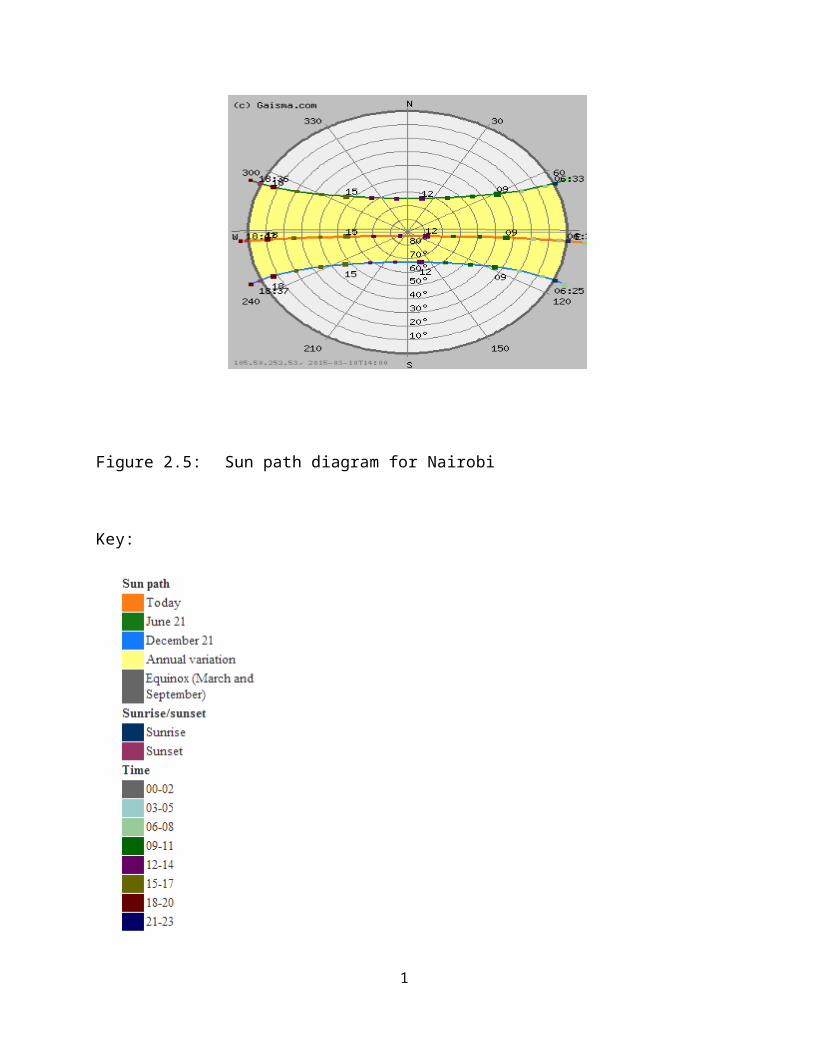
Figure 2.5: Sun path diagram for Nairobi
Key:

1313
Through the use of the chart, it is possible to ascertain the position of the sun at different times
and seasons so that the panel can be fixed for maximum output. Fixed trackers are cheaper in
tropical countries like Kenya. For countries beyond +10 degrees North and -10 degrees South
of the equator, there is need for serious tracking. This is because the position of the midday sun
varies significantly.
The chart shows that the position of the sun is highest between 1200h and 1400h. For the
periods outside this range, the collectors are obliquely oriented to the sun and therefore only a
fraction reaches the surface of absorption.
2.6.2 CASE I: The Fixed CollectorFor collectors that are fixed, the projection area on the area that is perpendicularly oriented to
the direction of radiation is given by S = So cos θ, where θ changes in the interval (-π/2, +π/2)
during the day. The angular velocity of the sun as it moves across the sky is given by ω =
2π/T =
7.27×10⁻⁵rad/s with the differential of the falling energy given by dW = ISdt. The energy per
unit that is calculated for the whole day neglecting atmospheric influence is given by:
ି�ଶଵ ω t ି�ଶଵ W = න IS୭ cos ωt dt = I S୭ sin ൨
2IS= , ()= 3.03 × 10W/m2
day
= 8.41 kWh/m2 day, (3)
�ିଶଵ ω ି�ଶଵ ω
2.6.3 Tracking collectors: Improvement of efficiencyFor tracking collectors, theoretical extracted energy is calculated assuming that maximum
radiation intensity I=1100W/m2 is falling on the area that is perpendicularly oriented to the
direction of radiation. There is comparison of intensity on the tracking collector and the
fixed one. More energy is gotten from the tracking collector than the fixed one.

1414
2.6.4 CASE II: The Tracking CollectorFor tracking collectors, if atmospheric influence is neglected, the energy per unit of area for an
entire day is given by
W = IS୭ t = 4.75 × 10Ws,
(4)

1414
= 13.2kWh/m2 day.(5)
Comparing the theoretical results for the two cases, more energy is obtained from the
second case, for the tracking collector. However, as the rays of the sun travel towards the earth,
they go through the thick layers of the atmosphere in both of the cases. That
notwithstanding, the tracking collector has more exposure to the sun’s energy at any given time.
2.7 Effect of light intensityChange of the light intensity incident on a solar cell changes all the parameters, including the
open circuit voltage, short circuit current, the fill factor, efficiency and impact of series and
shunt resistances. Therefore, the increase or decrease has a proportional effect on the amount of
power output from the panel.
2.8 Efficiency of solar panelsThe efficiency is the parameter most commonly used to compare performance of one solar
cells to another. It is the ratio of energy output from the solar panel to input energy from the
sun. in addition to reflecting on the performance of solar cells, it will depend on the spectrum
and intensity of the incident sunlight and the temperature of the solar cell. As a result,
conditions under which efficiency is to be measured must be controlled carefully to compare
performance of the various devices.
The efficiency of solar cells is determined as the fraction of incident power that is converted to
electricity. It is defined as:
[6]
where Voc is the open-circuit
voltage; Isc is the short-circuit
current
FF is the fill factor

1515
η is the efficiency.

1616
The input power for efficiency calculations is 1 kW/m2 or 100 mW/cm2. Thus the input
power for a 100 × 100 mm2 cell is 10 W.
2.9 Benefits and demerits of solar energyThere are several benefits that solar energy has and which make it favorable for many uses.
2.9.1 Benefits Solar energy is a clean and renewable energy source.
Once a solar panel is installed, the energy is produced at reduced costs.
Whereas the reserves of oil of the world are estimated to be depleted in future,
solar energy will last forever.
It is pollution free.
Solar cells are free of any noise. On the other hand, various machines used for
pumping oil or for power generation are noisy.
Once solar cells have been installed and running, minimal maintenance is required.
Some solar panels have no moving parts, making them to last even longer with no
maintenance.
On average, it is possible to have a high return on investment because of the free
energy solar panels produce.
Solar energy can be used in very remote areas where extension of the electricity
power grid is costly.
2.9.2 Disadvantages of solar power Solar panels can be costly to install resulting in a time lag of many years for savings
on energy bills to match initial investments.
Generation of electricity from solar is dependent on the country’s exposure to sunlight.
This means some countries are slightly disadvantaged.
Solar power stations do not match the power output of conventional power stations
of similar size. Furthermore, they may be expensive to build.
Solar power is used for charging large batteries so that solar powered devices can be
used in the night. The batteries used can be large and heavy, taking up plenty of space
and needing frequent replacement.

1717
Because merits are more than the demerits, the use of solar power is considered as a clean
and viable source of energy. The various limitations can be reduced through various ways.

1818
CHAPTER 3: DESIGN AND IMPLEMENTATION
3.1 Light Sensor Theory and Circuit of Sensor UsedLight detecting sensor that maybe used to build solar tracker include; phototransistors,
photodiodes, LDR and LLS05. A suitable, inexpensive, simple and easy to interface photo
sensor is analog LDR which is the most common in electronics. It is usually in form of a photo
resistor made of cadmium sulfide (CdS) or gallium arsenide (GaAs). Next in complexity
is the photodiode followed by the phototransistor [2].
3.2 Light Dependent Resistor Theory
The simplest optical sensor is a photon resistor or photocell which is a light sensitive resistor
these are made of two types, cadmium sulfide (CdS) and gallium arsenide (GaAs).
The sun tracker system designed here uses two cadmium sulfide (CdS) photocells for sensing
the light. The photocell is a passive component whose resistance is inversely proportional to
the amount of light intensity directed towards it. It is connected in series with capacitor.
The photocell to be used for the tracker is based on its dark resistance and light saturation
resistance. The term light saturation means that further increasing the light intensity to the CdS
cells will not decrease its resistance any further. Light intensity is measured in Lux, the
illumination of sunlight is approximately 30,000 lux [2].
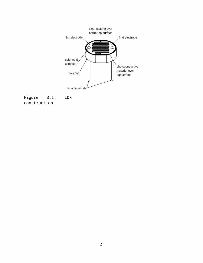
Figure 3.1: LDR construction

1919
Normally the resistance of an LDR is very high, sometimes as high as 1000 000 ohms, but
when they are illuminated with light resistance drops dramatically. When the light level is low
the resistance of the LDR is high. This prevents current from flowing to the base of the
transistors. Consequently the LED does not light. However, when light shines onto the LDR
its resistance falls.
3.2.1 The concept of using two LDRs
Figure 3.2: use of two LDRs
Concept of using two LDRs for sensing is explained in the figure above. The stable position is
when the two LDRs having the same light intensity.When the light source moves, i.e. the sun
moves from west to east, the level of intensity falling on both the LDRs changes and this
change is calibrated into voltage using voltage dividers. The changes in voltage are
compared using built-in comparator of microcontroller and motor is used to rotate the solar
panel in a way so as to track the light source.
3.3 Light sensor designThe solar tracker makes use of a Cds photocell for detecting light. There was use of a
complementary resistor with a value of 10k. With the resulting configuration, the output
voltage will increase with increase in light intensity. The value of the complementary resistor
is chosen

2020
such that the widest output range is achieved. The photocell resistance is measured under
bright light, average light and dark light conditions. The results are listed in the table below.
Table 3.1 Photocell Resistance Testing DataMeasured Resistance Comment
50 KΩ Dark light conditions (black vinyl tape placed
over cell)
4.35 KΩ Average light conditions (normal room lighting
level)
200 Ω Bright light conditions (flashlight directly in
front of cell)
The voltage divider circuit formed is shown below.
Figure 3.3: The input circuit that employs a voltage divider.

2020
From the given relationship, the input-output relationship for the voltage divider circuit is given
by:
V ୧ = Vୡୡ ൜ Rp o t ൠLDR + Rpot
In this case,
Vi =- input voltage into the microcontroller
R=Resistance of the [potentiometer which is10K
Vcc= Supply voltage to Microcontroller and
LDRs Vi=Input voltage to the Microcontroller
3.4 Servo motorServo motors are used for various applications. They are normally small in size and have good
energy efficiency. The servo circuitry is built inside the motor unit and comes with a
positionable shaft that is fitted with a gear. The motor is controlled with an electric signal that
determines the amount of shaft movement.
Figure 3.4: servo motor inside features
3.4.1 Components of the servo motorInside the servo there are three main components; a small DC motor, a potentiometer and a
control circuit. Gears are used to attach the motor to the control wheel. As the motor rotates,

2121
the resistance of the potentiometer changes so the control circuit can precisely regulate the
amount of movement there is and the required direction.

2222
When the shaft of the motor is at the desired position, power supply to the motor is stopped.
If the shaft is not at the right position, the motor is turned in the right direction. The
desired position is sent through electrical pulses via the signal wire. The speed of the motor is
proportional to the difference between the actual position and the position that is
desired. Therefore, if the motor is close to the desired position, it turns slowly. Otherwise, it
turns fast. This is known as proportional control [7].
3.4.2 How the servo is controlledServos are sent through sending electrical pulses of variable width, or pulse width modulation
(PWM), through the control wire. There is a minimum pulse, maximum pulse and a repetition
rate. Servos can usually turn only 90 degrees in either direction for a total of 180 degrees
movement. The neutral position of the motor is defined as that where the servo has the same
amount of potential rotation in both the clockwise and counter-clockwise direction. The PWM
sent to the motor determines the position of the shaft, and based on the duration of the pulse
sent through the control wire the rotor will turn to the position that is desired [7].
The servo motor expects to see a pulse after every 20 milliseconds and the length of the
pulse will determine how far the motor will turn. For instance, a 1.5ms pulse makes the motor
to turn in the 90 degrees position. If the pulse was shorter than 1.5ms, it will move to 0 degrees
and a longer pulse moves it to 180 degrees. This is shown below.
Figure 3.5: variable pulse width control servo position

2323
For applications where there is requirement of high torque, servos are preferable. They will also
maintain the torque at high speeds, up to 90% of the rated torque is available from servos at
high speeds. Their efficiencies are between 80 to 90%.
A servo is able to supply approximately twice their rated torque for short periods of
time, offering enough capacity to draw from when needed. In addition, they are quiet, are
available in AC and DC, and do not suffer from vibrations.
3.4.3 Advantages and disadvantages of servo motorsFor applications where high speed and high torque are required, servo motors are the
better option. While stepper motors peak at around 2000 RPM, servos are available at much
faster speeds. Servo motors also maintain torque at high speed, up to 90% of the rated
torque is available from servos at high speeds. They have an efficiency of about 80-90% and
supply roughly twice their rated torque for short periods. Furthermore, they do not vibrate or
suffer from resonance issues.
Servo motors are more expensive than other types of motors. Servos require gear boxes,
especially for lower operation speeds. The requirement for a gear box and position
encoder makes the designs more mechanically complex. Maintenance requirements will also
increase.
3.5 CrystalCrystal oscillators are electronic oscillator circuits that use inverse piezoelectric effect. With
this effect, when electric field is applied across certain materials they will produce
mechanical deformation. Therefore a crystal uses mechanical resonance of a vibrating crystal of
piezoelectric material so that there is creation of an electric signal with precise frequency. They
have high stability, are low cost and quality factor which makes them superior over such
resonators as LC circuits, ceramic resonators and turning forks.
The crystal action can be represented by an equivalent electrical resonant circuit.

2424
Figure 3.6 circuit diagram of a crystalThe optimal values of the capacitors depend on whether a quartz crystal or ceramic resonator
is being used. It will also depend on application-specific requirements on start-up time and
frequency tolerance. Crystal oscillators are not built into ICs because they cannot be easily
fabricated with IC processes and the size is physically larger than IC circuits.
The internal oscillators of microcontrollers are RC oscillators. The reason why crystal
oscillators are used is because the quality factor is on the order of 100000 while that of RC
oscillators is on the order of 100. Therefore, the crystal oscillator has lower phase noise and
lower variation in output frequency.
3.6 Voltage regulationVoltage regulators are designed to automatically maintain voltages at a constant level.
The LM7805 voltage regulator is used. It is a member of the 78xx series of fixed linear voltage
regulator ICs. Voltage sources in circuits could be having fluctuations and thus not be able
to give fixed voltage output. The voltage regulator IC maintains the output voltage at a value
that is constant. The LM7805 provides +5V regulated power supply. Capacitors are connected
at the input and output depending on respective levels of voltage [6].

2525
Figure 3.7: Voltage Regulator Circuit LM7805The pin diagram of the 7805 is shown below.
Figure 3.8: the LM7805 pin diagram
Table 3.2: Pin DescriptionPin No Function Name
1 Input voltage (5V-18V) Input
2 Ground (0V) Ground
3 Regulated output; 5V (4.8V-5.2V) Output
The maximum value for input to the voltage regulator is 35V. it also comes with a provision
for a heat sink. In cases where the voltage is near 7.5V there is no heat production and
therefore there is o need for a heat sink. If the voltage output is more, the excess
electricity will be liberated as heat.
2626
3.7 MicrocontrollerMicrocontroller is a single chip micro computer made through VLSI fabrication. A
microcontroller also called an embedded controller because the microcontroller and its support
circuits are often built into, or embedded in, the devices they control. A microcontroller is
available in different word lengths like microprocessors (4bit,8bit,16bit,32bit,64bit and 128 bit
microcontrollers are available today).
A microcontroller contains one or more of the following components:
Central processing unit (CPU)
Random Access Memory (RAM)
Read Only Memory (ROM)
Input/Output ports
Timers and Counters
Interrupt controls
Analog to digital converters
Digital analog converters
Serial interfacing ports
Oscillatory circuits
Microcontrollers need to be programmed to be capable of performing anything useful. It then
executes the program loaded in its flash memory – the code comprised of a sequence of
zeros and ones. It is organized in 12-, 14- or 16-bit wide words, depending on the
microcontroller’s architecture. Every word is considered by the CPU as a command being
executed during the operation of the microcontroller [1].

2727
Figure 3.9: Microcontroller Architecture
3.7.1 ATmega328PThe ATmega328P is a low-power CMOS 8-bit microcontroller based on the AVR
enhanced RISC architecture. By executing powerful instructions in a single clock cycle, the
ATmega328P achieves throughputs approaching 1 MIPS per MHz allowing the system
designer to optimize power consumption versus processing speed.
It has 28 pins. There are 14 digital I/O pins from which 6 can be used as PWM outputs and 6
analog input pins. The I/O pins account for 20 of the pins. The 20 pins can act as input to the
circuit or as output. Whether they are input or output is set in the software.
Two of the pins are for the crystal oscillator and are supposed to provide a clock pulse for the
Atmega chip. The clock pulse is needed for synchronization so that communication occurs in
synchrony between the Atmega chip and a device connected to it. Two of the pins, Vcc
and GND are for powering the chip. The microcontroller requires between 1.8-5.5V of power to
operate.
The pin-out for the microcontroller is shown

2828
below:

2929
Figure 3.10: Atmega 328P
The Atmega328 chip has an analog-to-digital converter (ADC) inside of it. This must be or
else the Atmega328 wouldn't be capable of interpreting analog signals. Because there is an
ADC, the chip can interpret analog input, which is why the chip has 6 pins for analog input.
The ADC has
3 pins set aside for it to function- AVCC, AREF, and GND. AVCC is the power supply,
positive voltage, that for the ADC. The ADC needs its own power supply in order to work.
GND is the power supply ground. AREF is the reference voltage that the ADC uses to convert
an analog signal to its corresponding digital value. Analog voltages higher than the reference
voltage will be assigned to a digital value of 1, while analog voltages below the reference
voltage will be assigned the digital value of 0. Since the ADC for the Atmega328 is a 10-bit
ADC, meaning it produces a 10-bit digital value, it converts an analog signal to its digital
value, with the AREF value being a reference for which digital values are high or low. Thus, a
portrait of an analog signal is shown by this digital value; thus, it is its digital correspondent
value [7].

3030
The last pin is the RESET pin. This allows a program to be rerun and start
over. The table below gives a description for each of the pins and their
functions.
Table 3.3 Pins and their functionsPin Number Description Function1 PC6 Reset2 PD0 Digital Pin (RX)3 PD1 Digital Pin (TX)4 PD2 Digital Pin5 PD3 Digital Pin (PWM)6 PD4 Digital Pin7 Vcc Positive Voltage (power)8 GND Ground9 XTAL 1 Crystal Oscillator10 XTAL 2 Crystal Oscillator11 PD5 Digital Pin (PWM)12 PD6 Digital pin (PWM)13 PD7 Digital pin14 PB0 Digital pin15 PB1 Digital pin (PWM)16 PB2 Digital pin (PWM)17 PB3 Digital pin (PWM)18 PB4 Digital pin19 PB5 Digital pin20 AVcc Positive voltage for ADC
(power)21 Aref Reference voltage22 GND Ground23 PC0 Analog input24 PC1 Analog input25 PC2 Analog input26 PC3 Analog input27 PC4 Analog input28 PC5 Analog input

3131
There are various features that make the ATmega 328P a good choice for the project:
Temperature Range:-40°C to 85°C Operating Voltage: 1.8 - 5.5V Low Power Consumption at 1 MHz, 1.8V, 25°C
Active Mode: 0.2 mA Power-down Mode: 0.1 µA Power-save Mode: 0.75
Special Microcontroller Features:
Power-on Reset and Programmable Brown-out Detection Internal Calibrated Oscillator External and Internal Interrupt Sources Six Sleep Modes: Idle, ADC Noise Reduction, Power-save, Power-down, Standby, and
Extended Standby
High Endurance Non-volatile Memory Segments
32K Bytes of In-System Self-Programmable Flash progam memory 1K Bytes EEPROM 2K Bytes Internal SRAM Write/Erase Cycles: 10,000 Flash/100,000 EEPROM Data retention: 20 years at 85°C/100 years at 25°C Optional Boot Code Section with Independent Lock Bits Programming Lock for Software Security
3.8 The design tool
Arduino IDEThe software design was done using Arduino IDE which was used for the programming. The
pargram was written using the C language. The Proteus circuit editing software was used for
drawing the PCB circuit. The design of the circuit was done using Eagle software.

3030
START
Initialize the System
Read values fromLDRs
Convert data from analog to digital
Calculate the angle of tilt andsend to Microcontroller
Compare the data
(S1-S2)>eGenerate drive signal forthe DC motor
(S2-S1)>e
STOP
Figure 3.11: A Simplified Flow Chart of the Assembly

3.9 Algorithm for Motor ControlThe algorithm gives the description of the general steps undertaken for the project:
1. There is input of the voltages from the two LDRs.
2. The inputs are analog. They are converted to digital values that range between 0-1023.
3. The two digital values are compared and the difference between them obtained.
4. The difference between the values obtained is the error proportional angle for the
rotation of the servo motor.
5. If the LDR voltages are the same, the servo stops. Otherwise, the servo rotates until
the difference is the same.
The flow chart of figure is an illustration of how the algorithm is implemented. The inputs
into the system are the two LDR voltages into pins 23 and 24 of the Atmega 328. There is
then the conversion of the analog voltages into their digital values. The larger of the two
signals is sent to the circuit which drives the DC motor to the direction with more light
intensity. The block diagram of the solar tracking system is shown below.
After that, all the components are assembled as is illustrated in the diagram below. The
input stage comprises the LDRs which feed the voltage outputs to the microcontroller. From the
LDRs are potentiometers that are used for varying the resistance. When there is plenty of
sunshine, the potentiometers are adjusted to their maximum value that is 10K. For days when
the weather is not very sunny, the resistance is reduced by varying the potentiometer to
ensure readings are more easily taken. The LDRs are connected to pins 4 and 5.
The embedded software design has the C code loaded into the Atmega 328P. The code that was
used is shown at the appendix of the report. The resistor R1 is a pull up resistor for
preventing the microcontroller from continually resetting.
Pins 8 and 22 are grounded as specified by the specifications of the microcontroller. Digital pin
9 is connected to the signal pin of the servo motor and serves to control the movement of the
servo. There is also the power pin of the servo that is connected to power. The last servo
pin is grounded. Pins 9 and 10 are for the quartz crystal. There are various switches that
control the powering of different components. The LED indicates when the circuit is powered

and the entire system is functional.
There is a reset button for positioning the panel to an initial position which is at an inclination of
40 degrees. This is done preferably in the evening after the sun has set. It makes the LDR go
back to an initial position, ready for tracking sunlight on the next day. There is also a push
button for initializing the servo motor. It switches it on, leaving it on standby mode.
Pins 7, 20 and 21 are for powering the microcontroller. It requires 5V. The inputs to the LDR
are simulated. The hardware schematic diagram is shown in figure
Figure3.12: Hardware schematic diagram

CHAPTER 4: RESULTS, SIMULATIONS AND ANALYSIS
4.1 ResultsThe results for the project were gotten from LDRs for the solar tracking system and the
panel that has a fixed position. The results were recorded for four days, recorded and tabulated.
The outputs of the LDRs were dependent on the light intensity falling on their surfaces.
Arduino has a serial that communicates on digital pins 0 (RX) and 1 (TX) as well as with the
computer through a USB. If these functions are thus used, pins 0 and 1 can be used for digital
input or output.
Arduino environment’s built in serial monitor can be used to communicate with the arduino
board. To collect the results, a code was written that made it possible to collect data from the
LDRs after every one hour. The values from the two LDRs are to be read and recorded at the
given intervals.
The LDRs measure the intensity of light and therefore they are a valid indication of the
power that gets to the surface of the solar panel. As a result, by measuring the light intensity at
a given time, it will be possible to get the difference in efficiency between the tracking panel
and the fixed one. The light intensity is directly proportional to the power output of the solar
panel.
A code was written that made it possible to obtain readings from the two LDRs at intervals
of one hour. The EEPROM came in handy in this. It is the memory whose values are kept when
the board is turned off. The ATmega 328P has 1024 bytes of EEPROM.
To get the values at the end of the day, the Arduino board was used to connect the
microcontroller to the computer. The RX and TX pins are used for the connection. The code
for reading the values that were recorded is loaded into the microcontroller. The various values
are obtained and converted into volts. The Vcc to the microcontroller and the LDRs is 5volts.
The Atmega 328P has 1024 voltage steps and 5volts. When they are converted into digital
values, the values will be in the range of 0-1023. The conversion is done using the relation
below.
LDR Output = ୯ ୳ ୧୴ୟ ୪ �ି୬ ୲ ୈ �ି ୧ ୧୲ ୟ୪ ୳ ୲ ୮୳ ୲ ∗ ହ
Volts

ଵଶଷ

The results were obtained for different days. Getting results from different days was helpful in
that it made it possible to compare the various values gotten from different weather
conditions. The values obtained were recorded and used to draw graphs to show the relations.
Table 4.1: Results for cloudy Morning and Sunny Afternoon for 6th and 7th April 2015
LDR readings for Fixed Panel LDR readings for a Tracking
Panel
Time LDR1 LDR2 LDR12 LDR22
0630Hrs 0.196 0.176 1.477 1.487
0730Hrs 0.249 0.210 1.804 1.839
0830Hrs 0.225 0.196 2.757 2.933
0930Hrs 0.723 0.567 3.631 3.783
1030Hrs 0.733 0.816 3.900 3.798
1130Hrs 3.211 2.297 3.910 3.969
1230Hrs 4.888 4.941 4.990 4.990
1330Hrs 3.803 3.910 4.985 4.990
1430Hrs 3.456 4.057 4.976 4.985
1530Hrs 3.930 3.846 4.941 4.892
1630Hrs 1.999 1.544 4.824 4.594
1730Hrs 1.090 1.144 3.128 2.981
1830Hrs 0.718 0.787 0.982 0.968

0630
Hrs
0730
Hrs
0830
Hrs
0930
Hrs
1030
Hrs
1130
Hrs
1230
Hrs
1330
Hrs
1430
Hrs
1530
Hrs
1630
Hrs
1730
Hrs
1830
Hrs
6
5
4
Volts (V) 3
2
1
0
LDR1
LDR2
LDR12
LDR22
Time (hourly)
Figure4.1: Graph of results obtained on 6th and 7th April
Table 4.2: LDR outputs for bright sunny day on 2nd April 2015
LDR readings for Fixed Panel LDR readings for a TrackingPanel
Time LDR1 LDR2 LDR12 LDR220630Hrs 0.679 0.489 1.477 1.4870730Hrs 0.792 1.061 2.804 2.8390830Hrs 1.779 1.672 3.203 3.9900930Hrs 3.167 1.199 3.990 3.9901030Hrs 3.421 3.226 4.130 4.1491130Hrs 4.604 3.208 4.500 4.5901230Hrs 4.990 4.980 4.990 4.9901330Hrs 4.980 4.990 4.888 4.9901430Hrs 4.888 4.941 4.976 4.9851530Hrs 4.413 3.878 4.941 4.8921630Hrs 3.935 3.824 4.873 4.7901730Hrs 2.639 2.639 3.964 3.9401830Hrs 1.569 1.031 2.708 2.815

0630
Hrs
0730
Hrs
0830
Hrs
0930
Hrs
1030
Hrs
1130
Hrs
1230
Hrs
1330
Hrs
1430
Hrs
1530
Hrs
1630
Hrs
1730
Hrs
1830
Hrs
6
5
4
Volts (V) 3
2
1
0
LDR1
LDR2
LDR12
LDR22
Time (hourly)
Figure 4.2: Graph for bright sunny day of 2nd April 2015
Table 4.3: Results for LDR outputs for a cloudy day on 12th April 2015LDR Readings for Fixed Panel LDR Readings for a Tracking
Panel
Time LDR1 LDR2 LDR12 LDR22
0630Hrs 0.147 0.117 0.274 0.244
0730Hrs 0.161 0.156 0.547 0.601
0830Hrs 0.274 0.205 1.090 1.075
0930Hrs 0.435 0.279 1.227 1.276
1030Hrs 0.572 0.547 1.271 1.305
1130Hrs 1.041 0.816 1.618 1.569
1230Hrs 2.175 1.965 2.165 2.151
1330Hrs 1.975 1.794 1.848 1.794
1430Hrs 1.119 1.623 1.090 1.075
1530Hrs 1.022 1.510 0.982 0.943
1630Hrs 0.543 1.017 0.762 0.728
1730Hrs 0.264 0.367 0.547 0.538
1830Hrs 0.064 0.103 0.327 0.220

0630
Hrs
0730
Hrs
0830
Hrs
0930
Hrs
1030
Hrs
1130
Hrs
1230
Hrs
1330
Hrs
1430
Hrs
1530
Hrs
1630
Hrs
1730
Hrs
1830
Hrs
6
5
4
Volts (V) 3
2
1
0
LDR1
LDR2
LDR12
LDR22
Time (hourly)
Figure 4.3: Graph of LDR outputs for a cloudy day on 12th April 2015Key points to note:
LDR1 is the photo resistor 1 reading for a solar panel that is
fixed. LDR2 indicates the 2nd photo resistor for a fixed solar
panel.
LDR 12 indicates the 1st photo resistor reading in the tracking solar panel.
LDR 22 indicates the 2nd photo resistor for a tracking solar panel.
4.2 AnalysisFrom the curves, it can be seen that the maximum sunlight occurs at around midday, with
maximum values obtained between 1200 hours and 1400 hours. In the morning and late
evening, intensity of sunlight diminishes and the values obtained are less that those obtained

during the day. After sunset, the tracking system is switched off to save energy. It is switched
back on in the morning.

For the panel fitted with the tracking system, the values of the LDRs are expected to be close.
This is because whenever they are in different positions there is an error generated that
enables its movement. The motion of the panel is stopped when the values are the same,
meaning the LDRs receive the same intensity of sunlight. For the fixed panel, the values vary
because the panel is at a fixed position. Therefore, at most times the LDRs are not facing the
sun at the same inclination. This is apart from midday when they are both almost perpendicular
to the sun.
Days with the least cloud cover are the ones that have the most light intensity and therefore
the outputs of the LDRs will be highest. For cloudy days, the values obtained for the tracking
system and the fixed system do not differ too much because the intensity of light is more
or less constant. Any differences are minimal. The tracking system is most efficient when it is
sunny. It will be able to harness most of the solar power which will be converted into energy.
In terms of the power output of the solar panels for tracking and fixed systems, it is evident
that the tracking system will have increased power output. This is because the power generated
by solar panels is dependent on the intensity of light. The more the light intensity the more
the power that will be generated by the solar panel.
The increase in efficiency can be calculated. However, it is important to note that there will be
moments when the increase in power output for the tracking system in comparison with the
fixed system is minimal, notably on cloudy days. This is expected because there will not be
much difference in the intensity of sunlight for the two systems. Similarly, on a very hot day at
midday, both systems have almost the same output because the sun is perpendicularly above.
As such, both systems receive almost the same amount of irradiation.
A few values can be used to illustrate the difference in efficiency between the two systems:
For a bright sunny day, we can take the averages for LDR22 and LDRS 2 for the entire day.
We then use 5 as the base because it is the maximum value of the LDR output. It is calculated
as a percentage and the two values compared. While this may not give the clearest indication of
the exact increase in efficiency, it shows that the tracking system has better efficiency.

averag e valu e o f L DR 2 2 o r L DR2 ∗ 1005 volts

For LDR 22:
4 .02 7 ∗ 100 = 80.54%5For LDR 2:
2 .85 6 ∗ 100 = 57.14%5The difference between the two values is 23.4%. this means the LDR for the tracking system
has an increased efficiency of 23.4%.

4040
CHAPTER FIVE: DISCUSSION, CONCLUSION AND RECOMMENDATIONS FOR FURTHER WORK
5.1 DiscussionThe objective of the project was to design a system that tracks the sun for a solar panel. This
was achieved through using light sensors that are able to detect the amount of sunlight that
reaches the solar panel. The values obtained by the LDRs are compared and if there is a
significant difference, there is actuation of the panel using a servo motor to the point where it
is almost perpendicular to the rays of the sun.
This was achieved using a system with three stages or subsystems. Each stage has its own role.
The stages were;
An input stage that was responsible for converting sunlight to a voltage.
A control stage that was responsible for controlling actuation and decision making.
A driver stage with the servo motor. It was responsible for actual movement of the panel.
The input stage is designed with a voltage divider circuit so that it gives desired range
of illumination for bright illumination conditions or when there is dim lighting. This
made it possible to get readings when there was cloudy weather. The potentiometer was
adjusted to cater for such changes. The LDRs were found to be most suitable for this project
because their resistance varies with light. They are readily available and are cost
effective. Temperature sensors for instance would be costly.
The control stage has a microcontroller that receives voltages from the LDRs and determines
the action to be performed. The microcontroller is programmed to ensure it sends a signal
to the servo motor that moves in accordance with the generated error.
The final stage was the driving circuitry that consisted mainly of the servo motor. The
servo motor had enough torque to drive the panel. Servo motors are noise free and are
affordable, making them the best choice for the project.

4141
5.2 ConclusionA solar panel that tracks the sun was designed and implemented. The required program was
written that specified the various actions required for the project to work. As a result,
tracking was achieved. The system designed was a single axis tracker. While dual axis trackers
are more efficient in tracking the sun, the additional circuitry and complexity was not required
in this case. This is because Kenya lies along the equator and therefore there are no significant
changes in the apparent position of the sun during the various seasons. Dual trackers are
most suitable in regions where there is a change in the position of the sun.
This project was implemented with minimum resources. The circuitry was kept simple, while
ensuring efficiency is not affected.
5.3 Recommendations for further workWith the available time and resources, the objective of the project was met. The project is able
to be implemented on a much larger scale. For future projects, one may consider the use of
more efficient sensors, but which are cost effective and consume little power. This would
further enhance efficiency while reducing costs. If there is the possibility of further reducing
the cost of this project, it would help a great deal. This is because whether or not such projects
are embraced is dependent on how cheap they can be.
Shading has adverse effects on the operation of solar panels. Shading of a single cell will have
an effect on the entire panel because the cells are usually connected in series. With
shading therefore, the tracking system will not be able to improve efficiency as is required.

4242
REFERENCES[1] A.K. Saxena and V. Dutta, “A versatile microprocessor based controller for
solar tracking,” in Proc. IEEE, 1990, pp. 1105 – 1109.
[2] T.A. Papalias and M. Wong, “Making sense of light sensors,”
h tt p: / /www . e m b e dd e d . c o m , 2006.
[3] R. Condit and D. W. Jones, “Simple DC motor fundamentals,” Texas
Instruments. Publication AN907, pp. 1 – 22, 2004.
[4] S. J. Hamilton, “Sun-tracking solar cell array system,” University of Queensland
Department of Computer Science and Electrical Engineering, Bachelors Thesis,
1999.
[5] M. F. Khan and R. L. Ali, “Automatic sun tracking system,” presented at the All
Pakistan Engineering Conference, Islamabad, Pakistan, 2005.
[6] “Fabrication of Dual-Axis Solar Tracking Controller Project”, Nader Barsoum, Curtin
University, Sarawak, Malaysia, Intelligent Control and Automation, 2011, 2, 57-68.
[7]Antonio L. Luque; Viacheslav M. Andreev (2007). Concentrator Photovoltaics. Springer
Verlag.
[8]David Cooke, "Single vs. Dual Axis Solar Tracking", Alternate Energy eMagazine, April
2011

4343
APPENDIXES
Appendix One: Code used in the microcontroller#include <Servo.h>
Servo tiltServo;
#define LDR1 A0 // LDR 1 pin#define LDR2 A1 // LDR 2 pin#define servoPin 9 // servo pin
long sumErrors = 0; // sum of errors for PIDlong wait = 0; // time between stepsuint8_t lastPosition = 0; // last servo positionint difference = 0; // difference between the two readingsboolean switchSides = false; // boolean variable to manage direction of rotationvolatile boolean commence = false; // starts the servo process
void setup() { Serial.begin(9600); tiltServo.attach(servoPin); attachInterrupt(0, initialize, RISING); attachInterrupt(1, activateServo, RISING);
}
void loop() {
int ldrValue1 = analogRead(LDR1); // get analog reading of LDR1 int ldrValue2 = analogRead(LDR2); // get analog reading of LDR2difference = ldrValue1 - ldrValue2; // calculate difference between the two values
if (commence){if ( difference >= -20 && difference <= 20 ){ Serial.println("e");lastPosition = tiltServo.read();
}else if (difference < -20){ if (switchSides){ sumErrors = 0;wait = 0;switchSides = false;
}tilt(1);
}else if (difference > 20){

4444
if (!switchSides){ sumErrors = 0; wait = 0;switchSides = true;
}tilt(0);
}}
//Serial.print("LDR1: "); Serial.println(ldrValue1);//Serial.print("LDR2: "); Serial.println(ldrValue2);Serial.print("Difference: "); Serial.println(difference);//Serial.print("Sum: "); Serial.println("sumErrors");//Serial.println("");
}
void tilt(boolean flag){int returnInt = 0; // holds PID valueif (flag && tiltServo.read() > 0){ // while servo is more than 0 degreestiltServo.write(lastPosition--); returnInt = PID(); delay(returnInt);
}else if (!flag && tiltServo.read() < 180){ // while servo less than 180 degrees tiltServo.write(lastPosition++);returnInt = PID();delay(returnInt);
}}
int PID(){wait = abs(difference) + abs(sumErrors); // PI controller. Assuming Kp and Ki are equal to 1 sumErrors += difference; // get the integral of errors
return(wait / 300); // return delay value}
void initialize(){ // go back to initial positionuint8_t pos = tiltServo.read(); // get current servo positionfor(uint8_t i = pos; pos > 30; pos--){ tiltServo.write(pos); // set servo positition delay(20);
}}

4545
void activateServo(){ // activate servo movement if (commence) commence = false;elsecommence = true;
}

4646
Appendix Two: Code for obtaining the results from the LDRs#include <EEPROM.h>#include <Servo.h>
Servo tiltServo;
#define LDR1 A0 // LDR 1 pin#define LDR2 A1 // LDR 2 pin#define servoPin 9 // servo pin
long sumErrors = 0; // sum of errors for PIDlong wait = 0; // time between stepsuint8_t lastPosition = 0; // last servo positionint difference = 0; // difference between the two readingsboolean switchSides = false; // boolean variable to manage direction of rotation int addr = 0;long time = 0;int ldrValue1 = 0;int ldrValue2 = 0;
void setup() { Serial.begin(9600); tiltServo.attach(servoPin); attachInterrupt(0, initialize, RISING);
}
void loop() {ldrValue1 = analogRead(LDR1); // get analog reading of LDR1 ldrValue2 = analogRead(LDR2); // get analog reading of LDR2 if (addr < 24)logData();difference = ldrValue1 - ldrValue2; // calculate difference between the two values
if (digitalRead(3) == HIGH){if ( difference >= -20 && difference <= 20 ){ Serial.println("equilibrium");lastPosition = tiltServo.read();
}else if (difference < -20){ Serial.println("turn left"); if (switchSides){ sumErrors = 0;wait = 0;switchSides = false;
}tilt(1);
}
4747
else if (difference > 20){ Serial.println("turn right"); if (!switchSides){ sumErrors = 0;wait = 0;switchSides = true;
}tilt(0);
}}//Serial.print("LDR1: "); Serial.println(ldrValue1);//Serial.print("LDR2: "); Serial.println(ldrValue2);Serial.print("Difference: "); Serial.println(difference);//Serial.print("Sum: "); Serial.println("sumErrors");//Serial.println("");
}
void tilt(boolean flag){int returnInt = 0; // holds PID valueif (flag && tiltServo.read() > 40){ // while servo is more than 0 degreestiltServo.write(lastPosition--); returnInt = PID(); delay(returnInt);
}else if (!flag && tiltServo.read() < 140){ // while servo less than 180 degrees tiltServo.write(lastPosition++);returnInt = PID();delay(returnInt);
}}
int PID(){wait = abs(difference) + abs(sumErrors); // PI controller. Assuming Kp and Ki are equal to 1 sumErrors += difference; // get the integral of errors
return(wait / 300); // return delay value}
void initialize(){ // go back to initial positionuint8_t pos = tiltServo.read(); // get current servo positionfor(uint8_t i = pos; pos > 40; pos--){ tiltServo.write(pos); // set servo positition delay(10);
}}//log data

4848
void logData(){time = millis()/1000;if (time >= 3600){EEPROM.write(addr, (float(ldrValue1)/4));addr++;EEPROM.write(addr, (float(ldrValue2)/4));addr++;time = 0;
}delay(10);
}

4949
Appendix Three: Code for obtaining the stored values of readings from the LDRs in Volts#include <EEPROM.h>
// start reading from the first byte (address 0) of the EEPROMint address = 0;byte value;
void setup(){
// initialize serial and wait for port to open: Serial.begin(9600);
}
void loop(){
while(address < 26){// read a byte from the current address of the EEPROMfloat value = float(EEPROM.read(address)) * 4;value = (value * 5)/1023; Serial.print(address); Serial.print("\t"); Serial.print(value); Serial.print("V"); Serial.println();
// advance to the next address of the EEPROMaddress = address + 1;
delay(500);}
}

Appendix Four: Screenshot of some of the readings obtained
50