Embed Size (px)
Citation preview
QUARTERLY OF APPLIED MATHEMATICSVOLUME LIII, NUMBER 2JUNE 1995, PAGES 259-271
EIGENFREQUENCIES OF CURVED EULER-BERNOULLIBEAM STRUCTURES WITH DISSIPATIVE JOINTS
By
WILLIAM H. PAULSEN
Arkansas State University, State University, Arkansas
Abstract. In this paper, we will compute asymptotically the eigenfrequencies forthe in-plane vibrations of an Euler-Bernoulli beam system with dissipative joints,which allow the beams to be curved into an arc of a circle. This enhances the au-thor's previous result for structures involving straight beams, given in his preprint"Eigenfrequencies of the non-collinearly coupled Euler-Bernoulli beam system withdissipative joints". Matrix techniques are used to combine asymptotic analysis witha form of the wave propagation method.
1. Introduction. In [14], a new method was introduced to find the in-plane vibra-tions of a general Euler-Bernoulli beam structure. For a straight beam, the beamequation is given by my n + EIyxxxx = 0, with 0 < x < L and / > 0. Here mdenotes mass density per unit length, and EI is the flexural rigidity of the beam. Foreach element of the structure, whether it be a bend, a length of beam, or a dissipativejoint, a corresponding 20 by 20 matrix was given. These matrices were multipliedtogether, along with a 1 by 20 matrix and a 20 by 1 matrix, to form a single equation.The eigenfrequencies could easily be computed asymptotically using this equation,and it was shown that, if the lengths of the beams were rational, there would be afinite number of "streams" of eigenfrequencies lying asymptotically close to a verticalline.
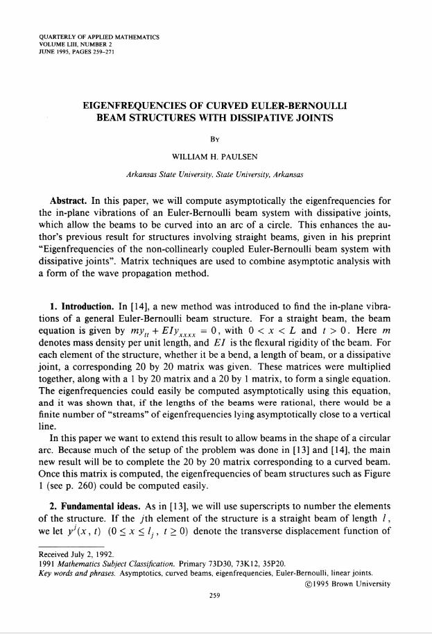
In this paper we want to extend this result to allow beams in the shape of a circulararc. Because much of the setup of the problem was done in [13] and [14], the mainnew result will be to complete the 20 by 20 matrix corresponding to a curved beam.Once this matrix is computed, the eigenfrequencies of beam structures such as Figure1 (see p. 260) could be computed easily.
2. Fundamental ideas. As in [13], we will use superscripts to number the elementsof the structure. If the yth element of the structure is a straight beam of length /,we let yJ (x, t) (0 < x < / , t > 0) denote the transverse displacement function of
Received July 2, 1992.1991 Mathematics Subject Classification. Primary 73D30, 73K.12, 35P20.Key words and phrases. Asymptotics, curved beams, eigenfrequencies, Euler-Bernoulli, linear joints.
©1995 Brown University259
260 WILLIAM H. PAULSEN
Fig. 1.
this beam. Since this is an Euler-Bernoulli beam, we have that
82 B4m—~yJ(x,t) + EI—jy\x,t) = 0 for 0 < x < / , />0. (2.1)
dt dx 'As in [13], we will make three simplifying assumptions for this model:(HI) The frame can vibrate only in the plane of the frame.(H2) The beams are essentially noncompressible, that is, the change of length of
the beams due to the forces exerted at the ends is negligible.(H3) Forces exerted on a beam in the direction parallel to the length of the beam
are propagated in a negligible amount of time.Because of assumption (H2), the longitudinal displacement is independent of the
position within a given beam. We let zJ(t) denote the longitudinal displacement ofthe yth beam. Also, because of assumption (H3), the longitudinal force of a givenbeam depends only on time; so we let HJ(t) denote the longitudinal force of the jthbeam.
To simplify the calculations, we will use the basis of [13], given in terms of thefollowing four functions:
IT , . cosh(x) + cos(x) ex + e,x + e~x + e~'xHya(x) = ^ = .
TT , , . sinh(x) - sin(x) ex + ie'x - e~x - ie~,xHyb(x) = = ,
TI . . cosh(x) - cos(x) ex - eix + e~x - e~'xHyc(x) = = ,
TI , sinh(x) + sin(x) ex - ie'x - e~x + ie~lxHyd(x) = ^= 4 •
We call these functions the "hybrid exponential functions". We can express thewave propagation in terms of the new functions:
y[{x , t) = (Aj Hya(?/x) + B} Hyb(^x)
+ C, Hyc{r]x) + D, Hyd(tix))e*'^7J™ ,/—— (2.2)
H[{t) = FjEIrfe
EIGENFREQUENCIES OF BEAM STRUCTURES 261
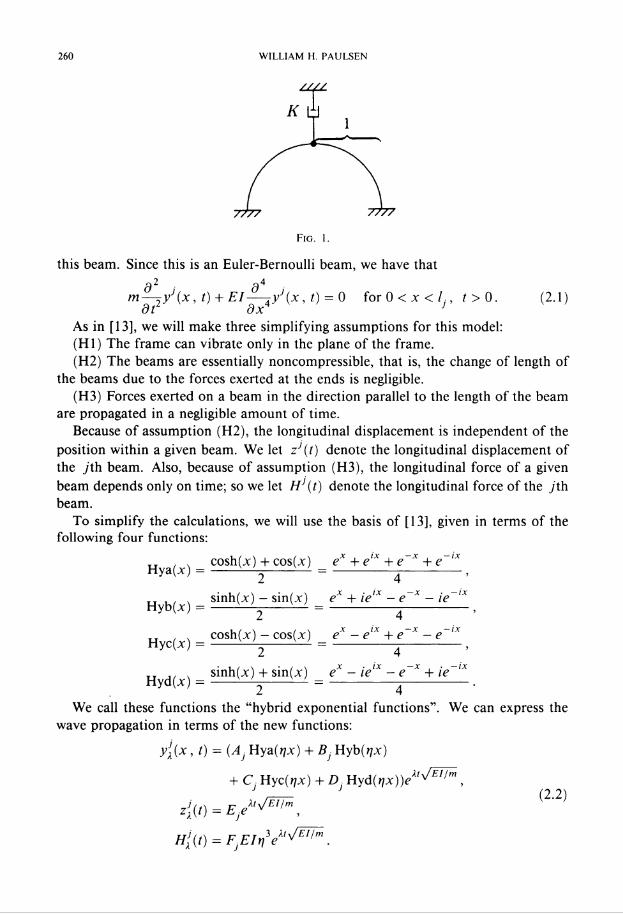
Fig. 2.
Here, rj = ^\/X, so that it/2 = X.The use of the hybrid exponentials deviates from the standard wave propagation
method (WPM) approach to the beam equation, as described in [8], Here, y[{x, t)was expressed as a linear combination of four "wave functions", namely, an incomingwave e('x+A'\/£//m) traveling to the right, another wave e^~lx+u\/EIlm^ traveling to
the left, and two evanescent waves e(x+x,y/E'/m'> an(j e(-x+ity/Ei/m) jast twQwaves decay exponentially fast in the x direction away from one of the endpoints.Thus, for each boundary condition encountered, one of the evanescent terms cansafely be discarded.
In (2.2), we are expressing the wave as a sum of four "hybrid waves". Each hybridwave is a linear combination of a wave traveling to the right, a wave traveling tothe left, and the two evanescent waves. At first this may seem like a disadvantage,since all four of the hybrid waves will be important at each juncture. However, thereflection and transmission relations will be greatly simplified. For example, if thebeginning end of the beam is clamped, as in the examples of [3] and [5], we canexpress the reflection relationships simply as AJ = D}. = 0. That is, two of the fourhybrid waves will not exist on that beam.
The price for using the hybrid wave functions is that the asymptotic estimationscannot immediately be employed by tossing out the evanescent waves. However, inthe case of a curved beam, it is not completely clear that such estimations could bemade anyway, since an evanescent wave may evolve into a different type of wave as ittransverses the curve. Thus, we must forgo all asymptotic analysis until we have theexact equation for the eigenfrequencies. Fortunately, the asymmetrical properties ofthe hybrid functions allow the results to be displayed.
The boundary conditions at each joint with a damper will depend on the type ofdamper involved. In [14], six different types of dampers are discussed, but we willonly need to understand the type III damper. Figure 2 demonstrates this type ofdamper. A single dashpot with a damping coefficient of K} is attached to the jointat a distance of r. from the center of the joint. The angle from the next beam to thedashpot is given by y.. If we draw a line from the point of contact of the dashpotto the center of the joint, the angle from the dashpot to this line is given by 5..
The boundary conditions for this joint are computed using linear approximationsto the angle displacement. For brevity, we will let v. = , Bj, C;, Dj, Ej, Fj) =the components of the wave in terms of the new basis after the y'th line in the
262 WILLIAM H. PAULSEN
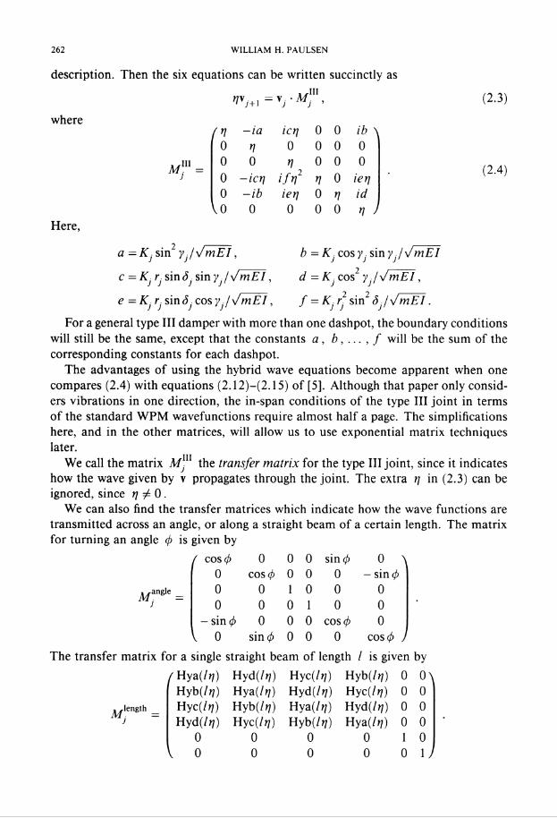
description. Then the six equations can be written succinctly as
V1=V^i?v,+1=v,-<\ (2.3)
where
JY111Mj =
ft] -ia ict] 0 0 ib \0 t] 0 0 0 0
o ° f 2 ° o ° • (2-4)0 -icq ijt] t] 0 let]0 —ib iet] 0 t] id
V0 0 0 0 0 rf )Here,
a = Kj sin y.fVmEI, b = K} cos y ■ sin y J VmEI
c = Kj r sin Sj sin y./VmEI, d = K. cos2 y}/VmEI,
e = Kj r sin SJ cos y./ VmEI, f — K] r sin2 8./ VmEI.
For a general type III damper with more than one dashpot, the boundary conditionswill still be the same, except that the constants a, b, ... , / will be the sum of thecorresponding constants for each dashpot.
The advantages of using the hybrid wave equations become apparent when onecompares (2.4) with equations (2.12)—(2.15) of [5], Although that paper only consid-ers vibrations in one direction, the in-span conditions of the type III joint in termsof the standard WPM wavefunctions require almost half a page. The simplificationshere, and in the other matrices, will allow us to use exponential matrix techniqueslater.
We call the matrix M™ the transfer matrix for the type III joint, since it indicateshow the wave given by v propagates through the joint. The extra tj in (2.3) can beignored, since t) 0 .
We can also find the transfer matrices which indicate how the wave functions aretransmitted across an angle, or along a straight beam of a certain length. The matrixfor turning an angle (f) is given by
( cos <j> 0 0 0 sin 0 0 \0 cos (f> 0 0 0 - sin q0 0 10 0 00 0 0 10 0
-sin 4> 0 0 0 cos 4> 0V 0 sin</> 0 0 0 cos (j> )
The transfer matrix for a single straight beam of length / is given by/Hya(/?/) Hyd (It]) Hyc (It]) Hyb (It]) 0 0\
Hyb(//?) Hya (Irj) Hyd (It]) Hyc(lt]) 0 0Hyc(lt]) Hyb (It]) Hya (It]) Hyd (It]) 0 0Hyd(/?;) Hyc (It]) Hyb (It]) Hya (It]) 0 0
0 0 0 0 10V 0 0 0 0 0 1J
Mangle
A/lcngth
EIGENFREQUENCIES OF BEAM STRUCTURES 263
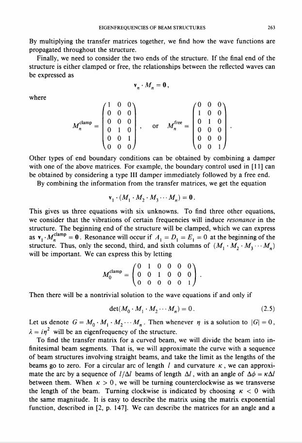
By multiplying the transfer matrices together, we find how the wave functions arepropagated throughout the structure.
Finally, we need to consider the two ends of the structure. If the final end of thestructure is either clamped or free, the relationships between the reflected waves canbe expressed as
y„-M= o,where
, ^clamp
(\ o o\0 0 00 0 00 1 00 0 1
V0 0 0 J
, ,freeor Mn =
/0 0 0\1 0 00 1 00 0 00 0 0
V0 0 1JOther types of end boundary conditions can be obtained by combining a damperwith one of the above matrices. For example, the boundary control used in [11] canbe obtained by considering a type III damper immediately followed by a free end.
By combining the information from the transfer matrices, we get the equation
v, • (A/, • M2 - M3 - ■ ■ Mn) = 0.
This gives us three equations with six unknowns. To find three other equations,we consider that the vibrations of certain frequencies will induce resonance in thestructure. The beginning end of the structure will be clamped, which we can expressas v1-M„clamp = 0 . Resonance will occur if A{ = D{ = = 0 at the beginning of thestructure. Thus, only the second, third, and sixth columns of (A/, • M2 ■ M3 ■ ■ ■ Mn)will be important. We can express this by letting
(0 1 0 0 0 0'^clamp = o o j 000yo o o o o 1
Then there will be a nontrivial solution to the wave equations if and only if
det(A/0 -A/, ■ M2 ■■■ Mn) = 0. (2.5)
Let us denote G = M0- ■ M2 - ■ ■ Mn . Then whenever t] is a solution to |G| = 0,A = irj will be an eigenfrequency of the structure.
To find the transfer matrix for a curved beam, we will divide the beam into in-finitesimal beam segments. That is, we will approximate the curve with a sequenceof beam structures involving straight beams, and take the limit as the lengths of thebeams go to zero. For a circular arc of length / and curvature k , we can approxi-mate the arc by a sequence of //A/ beams of length Al, with an angle of A</> = kAIbetween them. When k > 0, we will be turning counterclockwise as we transversethe length of the beam. Turning clockwise is indicated by choosing k < 0 withthe same magnitude. It is easy to describe the matrix using the matrix exponentialfunction, described in [2, p. 147], We can describe the matrices for an angle and a
264 WILLIAM H. PAULSEN
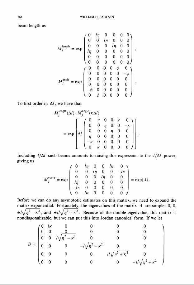
beam length as
, .-lengthMj = exp
, wangleMj — exp
To first order in A/, we have that
/ 0 It] 0 0 0 0^0 0/^0000 0 0 /1] 0 0h] 0 0 0 0 00 0 0 0 0 0
V 0 0 0 0 0 o7( 0 0 0 0 (f) 0 \
0 0 0 0 0 -00 0 0 0 0 00 0 0 0 0 0
-0 0 0 0 0 0V0 0000 0 7
= exp A/
Vength(A/) • M^(kAI)
( 0 //00k 0 \0 0 t] 0 0 —k0 0 0 ^0 0rj 0 0 0 0 0
—k 0 0 0 0 0Vo k 0 0 0 oy.
Including l/Al such beams amounts to raising this expression to the l/Al power,giving us
/ 0 It] 0 0 Ik 0 \0 0 It] 0 0 -Ik0 0 0 It] 0 0It] 0 0 0 0 0
-Ik 0 0 0 0 0V0 Ik 0 0 0 07
Before we can do any asymptotic estimates on this matrix, we need to expand thematrix exponential. Fortunately, the eigenvalues of the matrix A are simple: 0, 0,
, and ±il\Jt]2 + k2 . Because of the double eigenvalue, this matrix isnondiagonalizable, but we can put this into Jordan canonical form. If we let
(0 Ik 0 0 0 0 \0 0 0 0 0 0
, ^curveMj = exp = exp(.4)
D0 0 l\/t]2-K2 0 0 0
0 0 0 -l\Jt]2 -k2 0 0
0 0 0 0 ily/t]2 + K2 0
[o 0 0 0 0 t]2 + K2
and
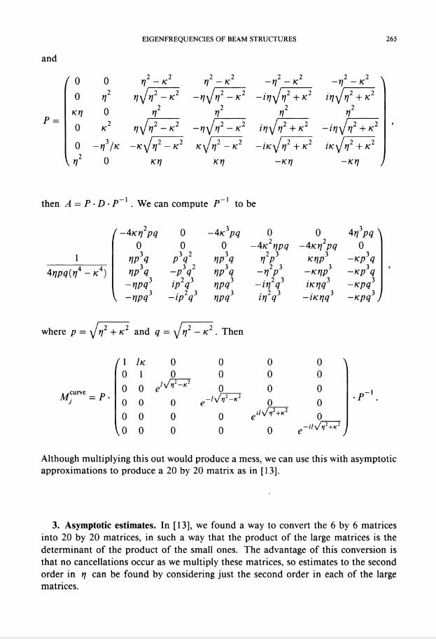
EIGENFREQUENCIES OF BEAM STRUCTURES 265
/ n n 2 2 2 2 2 2 2 2f 0 0 t] - k rj —k -rj -k -rj -k
0 t]2 t]\Jt]2 - k2 -r]\Jr}2 - K2 -it]\Jr\2 + k2 irj\f t]2 + k2a 2 2 2 2Kt] 0 t] t] t] t]
0 K2 t]\JT]2 - k2 -rj\Jt]2 - k2 it]\Jt]2 + k2 -ir]\Jrj2 + k0 -rj3/k -k\Jrj2 - k2 k\Jt]2 - k2 -iK\jt]2 + k2 iK\Jrj2 + k22 r,\ r] 0 Kt] KT] -KT] —Kt]
then A — P ■ D ■ P 1 . We can compute P 1 to be
4w(14-k4)
(-AKt]2pq 0 -4K^pq 0 0 4r?pq ^0 0 0 -4K2t]pq -AKt]2pq 03 32 3 23 3 3VP q P Q VP Q VP Kt]p -KP q3 323 23 3 3vp q -p q vp q -v p ~kvp -*p q
~vpq3 ip2q3 vpq3 ->v2q3 i*vq3 -*pq3 -23 3 -23 - 3 3,
~VPq ~ip q VPq 'V q -iKvq ~Kpq J
where p = \jt]2 + k2 and q — \jt]2 - k2 . Then
M;urve^p.
/1 Ik 0 0 0 00 1 0 0 0 0o o 0 0 00 0 0 ^-/vA/2-*2 p 0
0 0 0 0 o
P 1
Vo 0 0 0 0 e-''vV+K
Although multiplying this out would produce a mess, we can use this with asymptoticapproximations to produce a 20 by 20 matrix as in [ 13].
3. Asymptotic estimates. In [13], we found a way to convert the 6 by 6 matricesinto 20 by 20 matrices, in such a way that the product of the large matrices is thedeterminant of the product of the small ones. The advantage of this conversion isthat no cancellations occur as we multiply these matrices, so estimates to the secondorder in t] can be found by considering just the second order in each of the largematrices.
266 WILLIAM H. PAULSEN
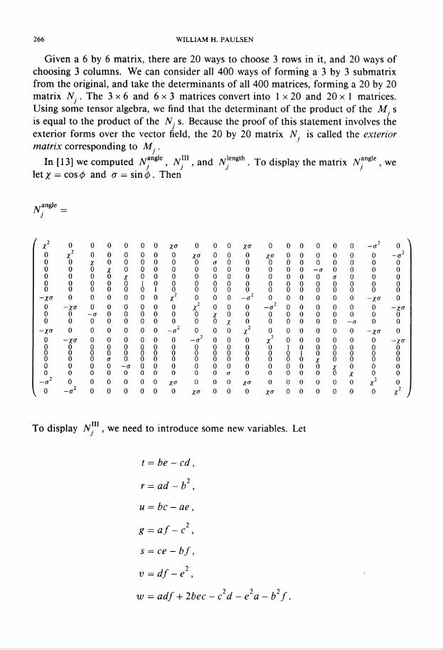
Given a 6 by 6 matrix, there are 20 ways to choose 3 rows in it, and 20 ways ofchoosing 3 columns. We can consider all 400 ways of forming a 3 by 3 submatrixfrom the original, and take the determinants of all 400 matrices, forming a 20 by 20matrix TV . The 3x6 and 6x3 matrices convert into 1 x 20 and 20 x 1 matrices.Using some tensor algebra, we find that the determinant of the product of the M. sis equal to the product of the Nj s. Because the proof of this statement involves theexterior forms over the vector field, the 20 by 20 matrix TV. is called the exteriormatrix corresponding to A/. .
In [13] we computed 7Vjngle, jV""1, and Arjcngth. To display the matrix A'J"8'0, welet x = cos <f> and a — sin (f>. Then
^y-angle _
( x1 0 0 0 0 0 0 *<7 0 0 0 *<r 0 0 0 0 0 0 -a1 0 ^0 X1 000000 *<r 0 0 0 x° 0 0 0 0 0 0 -a10 0 *00000 0 <t 0 0 000000 0 00 0 0/0000 0000 OOO-ctOO 0 00 0 00*000 0000 OOOOctO 0 00 0 000100 0000 000000 0 00 0 000010 0000 000000 0 0
-X" o 0 0 0 0 0 X2 o 00 -a1 0 00000 -*a 00 -xa 00000 0 X1 0 0 0 -a2 0 0 0 0 0 0 -*<r0 0 -a 0 0 0 0 0 0*00 000000 0 00 0 000000 00*0 00000 -a 0 0
-Xa 0 0 0 0 0 0 -tr2 0 0 0 *2 0 00000 -*cr 00 -xa 0 0 0 0 0 0 -a2 00 0 *2 00000 0 -*ct0 0 000000 0000 010000 0 00 0 000000 0000 001000 0 00 0 0 <t 0 0 0 0 0000 000*00 0 00 0 OO-uOOO 0000 0000*0 0 00 0 000000 OOctO 00000* 0 0
-a2 0 00000 *17 0 0 0 *cr 000000 *2 0000000 xa 0 0 0 0 0 0 0 0 0 *2
To display TV111, we need to introduce some new variables. Let
t — be - cd,
r = ad - b2,
u = be - ae,
g = af -e1,
s = ce - bf,
v =df-e2,
w = adf + 2bee - c2d - e2a - b2 f.
/
EIGENFREQUENCIES OF BEAM STRUCTURES 267
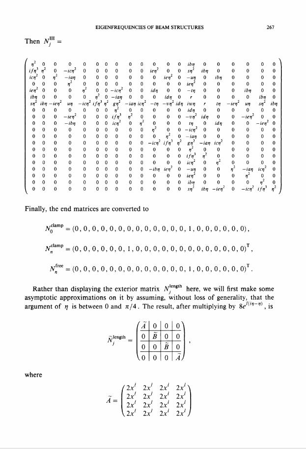
Then N™ =
/ 2 \n 0 o 0 0000 000 0 0 ibt] 0 0 0 0 00if I3 I2 o -icq2 0 0 0 0 0 0 iet]2 0 0 if/2 ibt] 0 0 0 0 0icr/2 0 t]1 —iat] 0 0 0 0 0 0 0 iet]2 0 —ut] 0 ibt] 0 0 0 0
000 t]2 0 000 000 00 iet]2 0 0 0 0 0 0iet]2 0 0 0 t]2 0 0 -iet]2 0 0 idt] 0 0 — tr] 0 0 0 ibr] 0 0ibt] 0 0 0 0 r/2 0 —iat] 0 0 0 idt] 0 r 0 0 0 0 ibt] 0
2 2 23222 2 2 2st] ibt] -iet] ut] -iet] iff] t] gt] -iar] iet] -tr] -vt] idr] iwt] r tr] -iet] ut] st] ibi]000 0 0 0 0 t]2 0 0 0 0 0 idt] 0 0 0 0 000 0 0 — iet]2 0 0 0 ifr? t]2 0 0 0 0 —vrf idt] 0 0 —iet]2 0 00 0 0 -ibr] 0 0 0 ictf 0 t]2 0 0 0 tr] 0 idt] 0 0 -iet]2 0000 0 0 000 00 t]2 00 -iet]2 0 0 0 0 0 0000 0 0 000 00 0 t]2 0 -iar] 0 0 0 0 0 0000 0 0 000 00 —iet]2 ift]3 r]2 gt]2 -iat] iet]2 0 0 0 0000 0 0 000 000 00 t]2 0 0 0 0 00000 0 0 000 000 0 0 if r/3 t]2 0 0 0 00000 0 0 000 000 00 icri2 0 t]2 0 0 0 0000 0 0 000 00 —ibr] iet]2 0 —ut] 0 0 t]2 -iat] ictf 0000 0 0 000 000 00 iet]2 0 0 0 t]2 0 0000 0 0000 000 0 0 ibt] 0 0 0 0 t]2 0000 0 0 000 000 00 st]2 ibt] -iet]2 0 — iet]2 iftf t]2
\ J
Finally, the end matrices are converted to
7V0clamp = (0, 0,0,0,0,0,0,0,0,0,0,0,0,1,0,0,0,0,0,0),
jVclamp = (0, 0, 0, 0, 0, 0,1,0, 0, 0, 0, 0, 0, 0, 0, 0, 0, 0, 0, 0)T,
7Vnfree = (0, 0, 0, 0, 0, 0, 0, 0, 0, 0, 0, 0, 0, 1, 0, 0, 0, 0, 0, 0)T.
Rather than displaying the exterior matrix Afjength here, we will first make someasymptotic approximations on it by assuming, without loss of generality, that theargument of t] is between 0 and n/A . The result, after multiplying by ''', is
Nj
(Alength 0
0vo
0B00
00B0
oAooa)
where
A
(2x 2xl 2xl 2xl \2xl 2xl 2x' 2xl2xl 2xl 2xl 2xl
V 2x' 2x 2xl 2xl)
268 WILLIAM H. PAULSEN
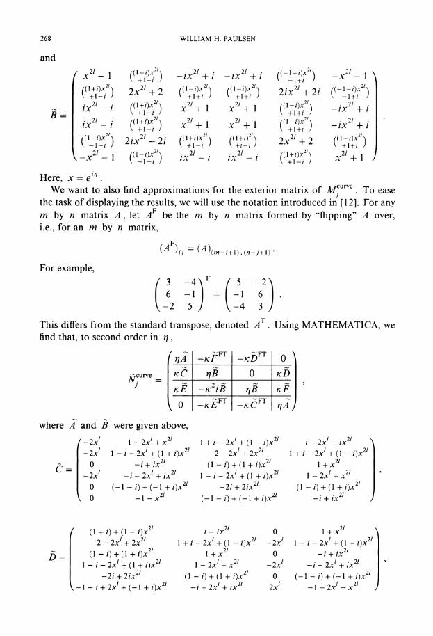
and
f x21 + \ ((1+1+f) -ix2' + i -ix2' + i -x21 - \ }
((+i-f) 2x2' + 2 («;[£) ((1+7if) -2ix21 + 2i ^f)ix2' -1 (C+'lf) x2, + l x2l+l (""'if) -ix21 + ic2/-/ ((1++;lf) x2/ + i x2/ + i ((1;;}f) -/x2/ + i
B =
2«2'-2/ (»«»',) CiA) 2.v%2 ("-'11 )V-JC2/-I C'-'lf) /jc2' - (' ijc2' — / ("^f) x2/+l 7
Here, x = e'n .We want to also find approximations for the exterior matrix of AfJurve. To ease
the task of displaying the results, we will use the notation introduced in [12], For anym by n matrix A, let AFi.e., for an m by n matrix,
pm by n matrix A, let A be the m by n matrix formed by "flipping" A over,
(Aj = (A)(m—i+l), (n—j+i) '
For example,
TThis differs from the standard transpose, denoted A . Using MATHEMATICA, wefind that, to second order in q,
/
^curve
rjAkC
kE
\ o
PFT-kFriB
-k2IB£FT-kE
^FT-kD
riB-kC"
0 XkD
kF
where A and B were given above,
r -2x' 1 — 2x' + x2' 1 + / - 2x1 + (1 - ;)x2' i — 2x1 — ix21 ^-2x' 1 - i - 2x' + (1 + i)x2' 2 - 2x + 2x11 1 + i - 2x' + (1 - i)x21
c =
D
0 -/ + ix21 (1 - 0 + (1 + i)x2' 1 + x2'—2x —i - 2x' + ix21 1 — i — 2xl + (1 + i)x21 1 - 2xl + x21
0 (-1 -/') + (-1 + i)x2' -2 i + 2 ix2' (1 -;) + (1 + i)x2'V 0 -1-x2' (-1 -/) + (-! +i)x2' -i + ix2' 7
(1 + /) + (1 - i)x21 i - ix21 0 1 + x21 ^2 — 2x1 + 2x21 1 + i — 2xl + (1 - i)x2' —2xl I — / — 2xl + (1 + i)x21
(1 - i) + (1 + i)x2' \+x2' 0 - i + ix211 - i - 2x + (1 + i)x21 1 - 2x' + x2' -2x' —/' - 2x' + ix21
-2/ + 2/X2' (1-/) + (!+;)x2/ 0 (-1 - ;) + (-1 + i)x11V — 1 — / + 2x' + (-1 + ; )x2/ + 2x' + ix21 2xl -1 + 2x' - x2'
EIGENFREQUENCIES OF BEAM STRUCTURES 269
-i + ix2' (1 - i) + (1 + i)x21 1 + x2' 0 ^
(-1-
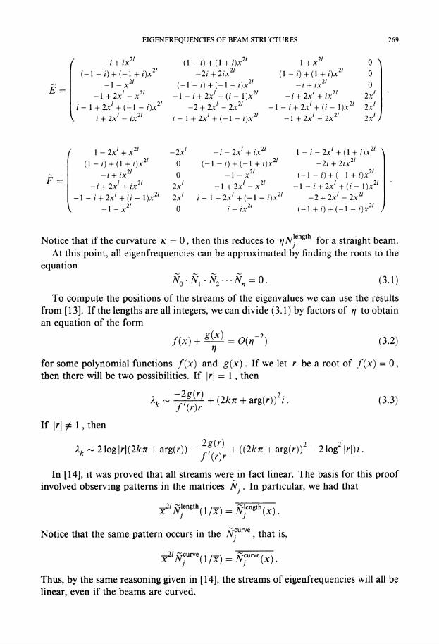
E =
(—1 - i) + (-1 + i)x21 —2i + 2ix21 (1 —/) + (1 +i)x21 0-l-x21 (— 1 - i) + (-1 + i)x21 —i+ix21 0
-1 + 2x' — x21 — 1 — i + 2xl + (/ — 1 )x21 -i + 2xl + ix21 2xli - \ + 2x +{ - \ - i)x2' -2 + 2x'-2x21 -1 - i + 2x' + (< -\)x2' 2xl
i + 2x1 - ix2' i - 1 + 2x' + (-1 - i)x21 -1 + 2x - 2x21 2x1 J
1 — 2x + x21 -2x —i — 2xl + ix21 1 — i — 2x' + (1 + i)x21 ^(1 - i) + (l + i)x2' 0 (-1 -/') + (-1 +i)x21 -2i + 2ix1'
—i + ix21 0 -1 - x21 (— 1 — i) + (— 1 + i)x21-i + 2x' + ix21 2x1 -1 + 2x' - x21 — 1 — i + 2x' + (/ — 1 )x21
— 1 - i + 2xl + (i - \)x2' 2x' i — 1 + 2xl + (-1 - i)x21 -2 + 2xl - 2x21-l-x21 0 i - ix21 (-1 + i) + (-1 — i)x21 )
Notice that if the curvature k — 0, then this reduces to t] Vength for a straight beam.At this point, all eigenfrequencies can be approximated by finding the roots to the
equation
N0-NrN2-.-Nn = 0. (3.1)To compute the positions of the streams of the eigenvalues we can use the results
from [13]. If the lengths are all integers, we can divide (3.1) by factors of t] to obtainan equation of the form
m + ~ = 0(^2) (3-2)
for some polynomial functions f(x) and g(x). If we let r be a root of f(x) = 0,then there will be two possibilities. If |r| = 1, then
xk ~ r'fV + (2kn + afg(r))2/ • (3-3)J \r)r
If |r| ^ 1, then
~ 2\og\r\(2kn + arg(r)) - + {(2kn + arg(r))2 - 2log2 |r|)/./ (r)r
In [14], it was proved that all streams were in fact linear. The basis for this proofinvolved observing patterns in the matrices Nf. In particular, we had that
_2/^length( j/_) = Mength^^J K ' ' J
Notice that the same pattern occurs in the Ar|urve, that is,
x2/7Vcurve(l/x) = NjUrve(x).
Thus, by the same reasoning given in [14], the streams of eigenfrequencies will all belinear, even if the beams are curved.

270 WILLIAM H. PAULSEN
As an example, we can use the large matrices to find the approximate eigenfre-quencies of the structures in Figure 1. For simplicity, we will take mEI = 1 . Inthis case, the damper is a type III, with a = K and b = c = d — e — f = 0. Aftermultiplying the matrices together, and dividing by a factor of ^ , we obtain (3.2),with
/(x) = -87i(l + x2n)
andg{x) = - 4 - 4/ + (2 + 2i)Kn + (16 + 16i)x*12 - 40** + 4iKjtx"
+ (16 - 16/)x3?r/2 + (-4 + 4i)x2n + (-2 + 2i)Knx2n .
Since the lengths of the beams were not rational, f(x) and g(x) are not polynomialsin x. However, we can change variables to make them polynomials. If we letr\ = nrj/2 and x = e'n = x^2, then (3.2) becomes
f(x') + ^ = 0(rj'~2)t]with
f(x') = —8tt( 1 -I- x'4)and
g(x') = (-2 - 2i)n + (1 + i)Kn2 + (8 + 8 i)nx - 20nx'~ + 2iKn x2
+ (8 - 8/)7ix'3 + (-2 + 2i)nx'A + (-1 + i)Kn2x'4.
We can apply (3.3) to obtain an estimate for it]2. We obtain the four linear streams
inA //-,_> . _ , .s21 ,k ((2nk + n/4) + 3/2 - ^2 - Kn/8)i,
in'2 k ~ - Kn/4 + ((2nk + 3n/4)2 - 1 - Kn/S)i,
in'2 k ~ ({Ink + Sn/4)1 + 3/2 + sfl - Kn/S)i,
ink ~ - Kn/4 + ((2nk + In/4)" - 1 - Kn/S)i.2 / 2Since X = it] = 4it] /it , we have
Xx k ~ ((4k + \/2)2 + 6/n2 -4^2/n2 - K/2n)i,
X2 k ~ - K/n + ((4k + 3/2)2 — 4/n2 - K/2n)i,
X3tk ~ ((4A: + 5/2)2 + 6/^2 + 4\/2/7r2 - A"/2tc)i,
~ - K/n + ((4k + 7/2)2 - 4/n2 - K/2n)i.Much of the work in this paper required the use of the symbolic manipulator
MATHEMATICA running on a SUN Microsystems workstation for the computationof the large matrices.
Although this paper analyzes a linear model of a physical system, the experimentaldata cited in [5] and [6] indicate that this model is an accurate one. However, westill are only considering vibrations that occur within the plane. Hopefully, analysisfor structures that do not lie in a plane can be done using a similar technique, andthis will be treated in a future work.
EIGENFREQUENCIES OF BEAM STRUCTURES 271
References
[1] C. Aganovic and Z. Tutez, A justification of the one-dimensional model of an elastic beam, Math.Methods Appl. Sci. 8, 1 -14 (1986)
[2] W. Boothby, An Introduction to Differentiable Manifolds and Riemannian Geometry, AcademicPress, Orlando, FL, 1986
[3] G. Chen, M. C. Delfour, A. M. Krall, and G. Payne, Modeling, stabilization, and control of seriallyconnected beams, SIAM J. Control Optim. 25, 526-546 (1987)
[4] G. Chen, S. G. Krantz, D. W. Ma, C. E. Wayne, and H. H. West, The Euler-Bernoulli beamequation with boundary energy dissipation, Operator Methods for Optimal Control Problems,Marcel Dekker, New York, 1987, pp. 67-96
[5] G. Chen, S. G. Krantz, D. L. Russell, C. E. Wayne, H. H. West, and M. P. Colman, Analysis,designs and behavior of dissipative joints for coupled beams, SIAM J. Appl. Math. 49, 1665-1693(1989)
[6] G. Chen, S. G. Krantz, D. L. Russell, C. E. Wayne, H. H. West, and J. Zhou, Modeling, analysisand testing of dissipative beam joints—experiments and data smoothing, Math. Comput. Modelling11, 1011-1016 (1988)
[7] G. Chen and H. Wang, Asymptotic locations of eigenfrequencies of Euler-Bernoulli beam withnonhomogeneous structural and viscous damping coefficients, SIAM J. Control Optim. 29, 347-367(1991)
[8] G. Chen and J. Zhou, The wave propagation method for the analysis of boundary stabilization invibration structures, SIAM J. Appl. Math. 50, 1254-1283 (1990)
[9] P. G. Ciarlet, Plates and Junctions in Elastic Multi-structures, Springer-Verlag, New York, 1990[10] J. B. Keller and S. I. Rubinow, Asymptotic solution of eigenvalue problems, Ann. of Physics 9,
24-75 (1960)[11] A. M. Krall, Asymptotic stability of the Euler-Bernoulli beam with boundary control, J. Math. Anal.
Appl. 137, 288-295 (1989)[12] S. G. Krantz and W. Paulsen, Asymptotic eigenfrequency distributions for the N-beam Euler-
Bernoulli coupled beam equation with dissipative joints, J. Symbolic Comput. 11, 369-418 (1991)[13] W. H. Paulsen, Eigenfrequencies of non-collinearly coupled beams with dissipative joints, Proc. 31 st
IEEE Conf. Decision and Control (Tucson, AZ, 1992), Vol. 3, IEEE Control Systems Soc., NewYork, 1992, pp. 2986-2991
[14] W. H. Paulsen, Eigenfrequencies of the non-collinearly coupled Euler-Bernoulli beam system withdissipative joints, preprint
[15] W. D. Pilkey, Manual for the response of structural members. Vol. I, Illinois Inst. Tech. Res. Inst.Project J6094, Chicago, IL, 1969