Embed Size (px)
Citation preview
Digital Image Processing: Bernd Girod, © 2013 Stanford University -- Eigenimages 1
Eigenimages
n Unitary transformsn Karhunen-Loève transform and eigenimagesn Sirovich and Kirby methodn Eigenfaces for gender recognitionn Fisher linear discrimant analysisn Fisherimages and varying illuminationn Fisherfaces vs. eigenfaces
Digital Image Processing: Bernd Girod, © 2013 Stanford University -- Eigenimages 2
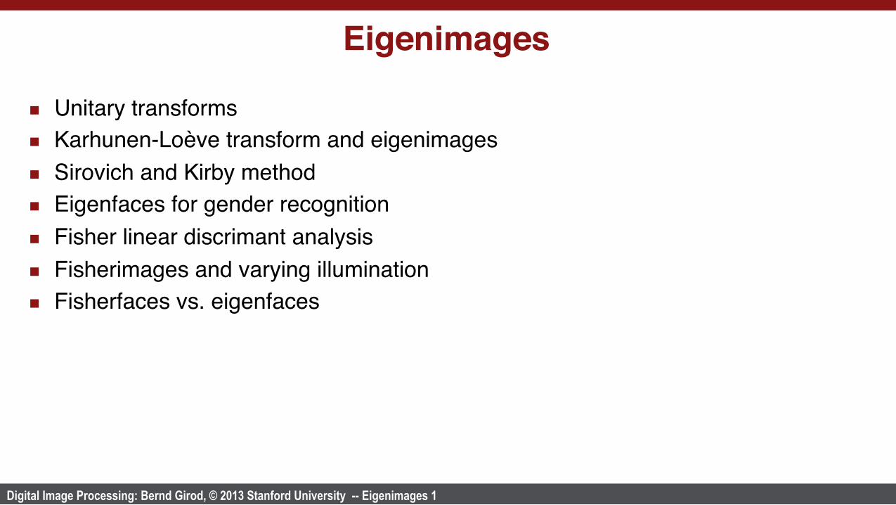
Unitary transforms
n Sort pixels f [x,y] of an image into column vector of length Nn Calculate N transform coefficients
where A is a matrix of size NxNn The transform A is unitary, iff
n If A is real-valued, i.e., A=A*, transform is „orthonormal“
c = A
f
A−1 = A*T ≡ AH
Hermitian conjugate
!f

Digital Image Processing: Bernd Girod, © 2013 Stanford University -- Eigenimages 3
Energy conservation with unitary transforms
n For any unitary transform we obtain
n Interpretation: every unitary transform is simply a rotation of the coordinate system (and, possibly, sign flips)
n Vector length is conserved.n Energy (mean squared vector length) is conserved.
c = A
f
c 2 = cH c =
f H AHA
f =f2
Digital Image Processing: Bernd Girod, © 2013 Stanford University -- Eigenimages 4
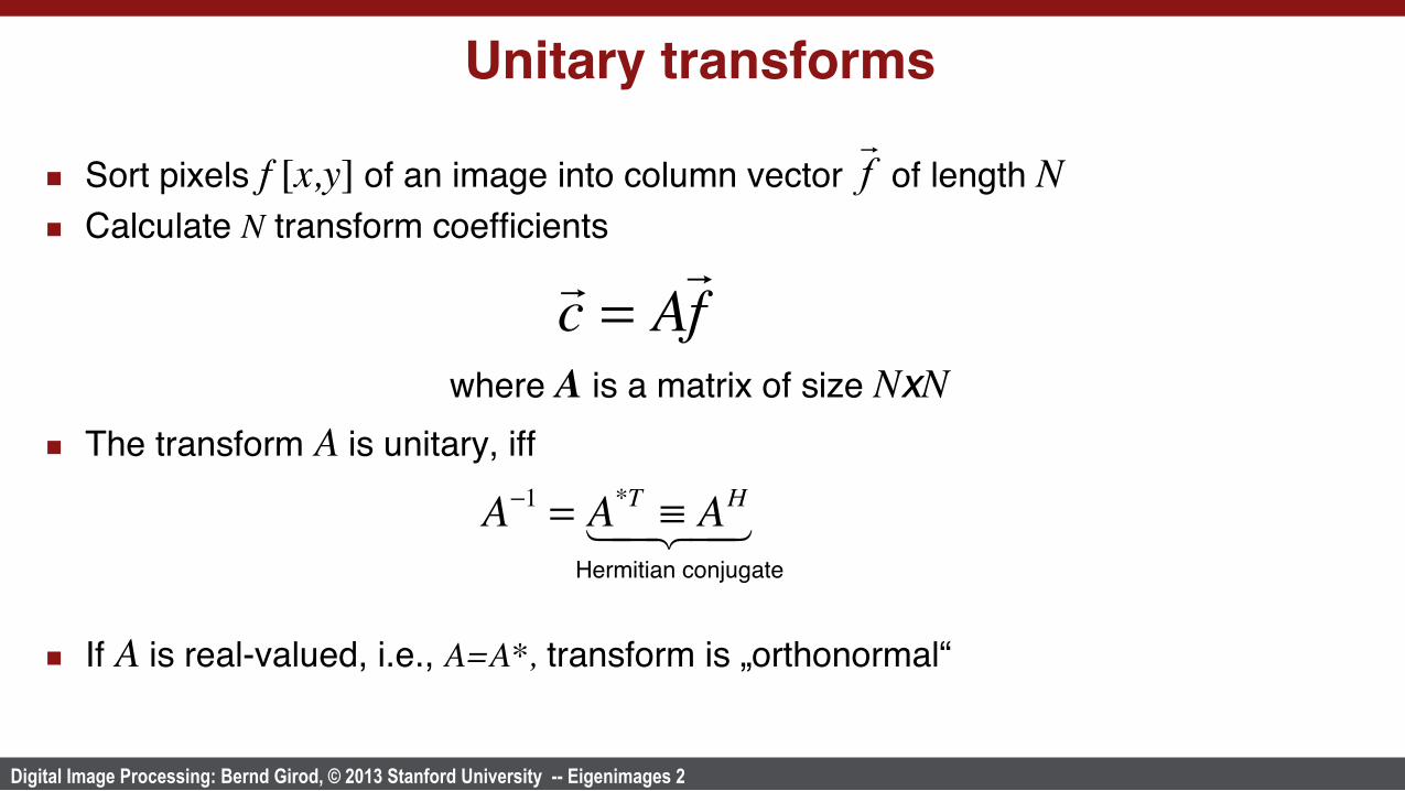
Energy distribution for unitary transforms
n Energy is conserved, but, in general, unevenly distributed among coefficients.n Autocorrelation matrix
n Diagonal of Rcc comprises mean squared values („energies“) of the coefficients ci
n for now: assume Rff is known or can be computed
Rcc = E cc H⎡⎣ ⎤⎦ = E A
f ⋅f H AH⎡⎣ ⎤⎦ = ARff AH
E ci
2⎡⎣ ⎤⎦ = Rcc⎡⎣ ⎤⎦i,i= ARff AH⎡⎣ ⎤⎦i,i

Digital Image Processing: Bernd Girod, © 2013 Stanford University -- Eigenimages 5
Eigenmatrix of the autocorrelation matrix
Definition: eigenmatrix Φ of autocorrelation matrix Rff
l Φ is unitaryl The columns of Φ form a set of eigenvectors of Rff, i.e.,
Λ is a diagonal matrix of eigenvalues λi
l unitary eigenmatrix for auto-correlation matrix always exists
l Rff is symmetric positive (semi-)definite, hence
RffΦ = ΦΛ
Λ =
λ0 0
λ1
!0 λN−1
$
%
&&&&&
'
(
)))))
λi ≥ 0 for all i

Digital Image Processing: Bernd Girod, © 2013 Stanford University -- Eigenimages 6
Karhunen-Loève transform
n Unitary transform with matrix
n Transform coefficients are pairwise uncorrelated
n Columns of Φ are ordered according to decreasing eigenvalues.n Energy concentration property:
l No other unitary transform packs as much energy into the first J coefficients.l Mean squared approximation error by keeping only first J coefficients is minimized. l Holds for any J.
A = ΦH
Rcc = ARff AH = ΦH RffΦ = ΦHΦΛ = Λ
Digital Image Processing: Bernd Girod, © 2013 Stanford University -- Eigenimages 7
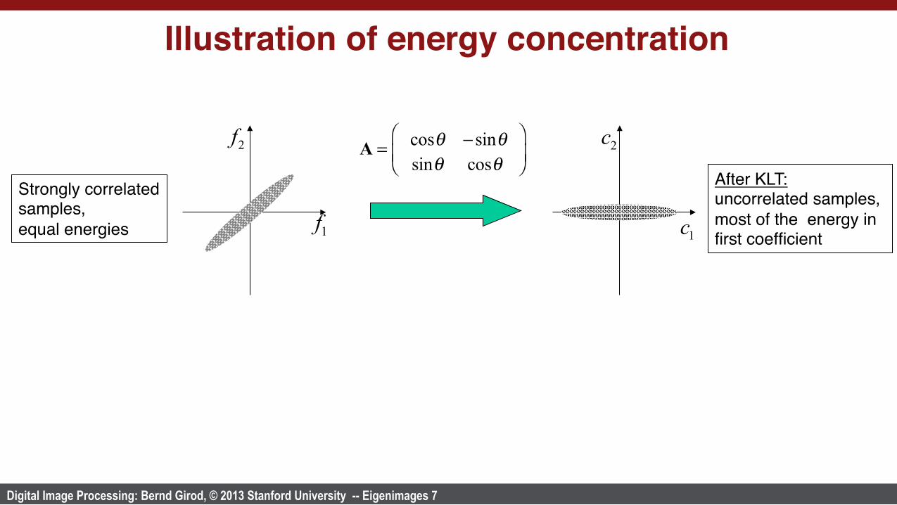
Illustration of energy concentration
1f
2f
1c
2c
Strongly correlated samples, equal energies
After KLT:uncorrelated samples, most of the energy in first coefficient
A = cosθ − sinθ
sinθ cosθ
⎛
⎝⎜⎞
⎠⎟

Digital Image Processing: Bernd Girod, © 2013 Stanford University -- Eigenimages 8
Basis images and eigenimages
n For any transform, the inverse transform
can be interpreted in terms of the superposition of columns of A-1 („basis images“)n For the KL transform, the basis images are the eigenvectors of the
autocorrelation matrix Rff and are called „eigenimages.“n If energy concentration works well, only a limited number of eigenimages is
needed to approximate a set of images with small error. These eigenimages span an optimal linear subspace of dimensionality J.
!f = A−1!c
Digital Image Processing: Bernd Girod, © 2013 Stanford University -- Eigenimages 9
n To recognize complex patterns (e.g., faces), large portions of an image have to be considered
n High dimensionality of “image space” means high computational burden for many recognition techniquesExample: nearest-neigbor search requires pairwise comparison with every image in a database
n Transform can reduce dimensionality from N to J by representing the image by J coefficients
n Idea: tailor a KLT to a specific set of training images representative of the recognition task to preserve the salient features
c =W
f
Eigenimages for recognition

Digital Image Processing: Bernd Girod, © 2013 Stanford University -- Eigenimages 10
Normalization
f
f
Projection
f
Database of Eigenface
Coefficients
Mean Face
+ -
p1…
…
…
… …
!pK
Similarity measure
(e.g., )
Class of most similar
Similarity Matching
New Face Image
×k *
RecognitionResult
Rejection
1
W f
c
pk
θ !cT !pk*
Eigenimages for recognition
Digital Image Processing: Bernd Girod, © 2013 Stanford University -- Eigenimages 11
Computing eigenimages from a training set
n How to obtain NxN covariance matrix?l Use training set (each column vector represents one image)l Let be the mean image of all L+1 training imagesl
Problem 1: Training set size should be
Problem 2: Finding eigenvectors of an NxN matrix.
n Can we find a small set of the most important eigenimages from a small training set ?
Define training set matrix S =!Γ1 − µ"!
,!Γ2 − µ"!
,!Γ3 − µ"!
,…,!Γ L − µ
"!( ),
and calculate scatter matrix R =!Γ l − µ"!
( )l=1
L
∑!Γ l − µ"!
( )H= SS H
L+1>> N If L < N, scatter matrix R is rank-deficient
!Γ1,!Γ2 ,…,
!Γ L+1
L << N
µ

Digital Image Processing: Bernd Girod, © 2013 Stanford University -- Eigenimages 12
Sirovich and Kirby algorithm
n
n
n
Sirovich and Kirby Algorithm (for ) l Compute the LxL matrix SHS l Compute L eigenvectors of SHS l Compute eigenimages corresponding to the largest eigenvalues
as a linear combination of training images
Instead of eigenvectors of SS H , consider the eigenvectors of S H S, i.e.,
S H Svi = λi
vi
Premultiply both sides by S SS H Svi = λiS
vi
By inspection, we find that Svi are eigenvectors of SS H
L << N
vi
L0 ≤ L
Svi
L. Sirovich and M. Kirby, "Low-dimensional procedure for the characterization of human faces," Journal of the Optical Society of America A, 4(3), pp. 519-524, 1987.
SS H S!vi = λiS!vi
Digital Image Processing: Bernd Girod, © 2013 Stanford University -- Eigenimages 13
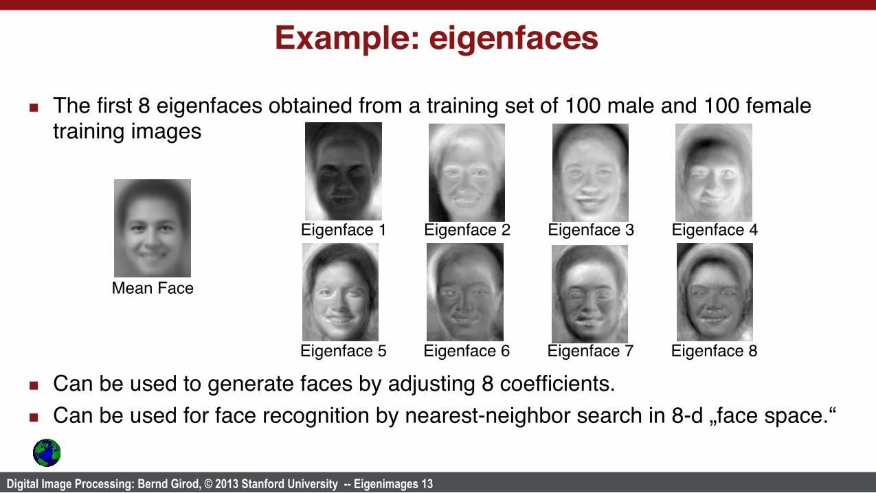
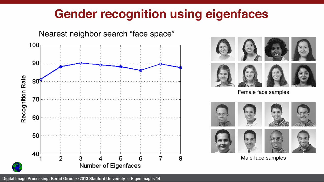
Example: eigenfaces
n The first 8 eigenfaces obtained from a training set of 100 male and 100 female training images
n Can be used to generate faces by adjusting 8 coefficients.n Can be used for face recognition by nearest-neighbor search in 8-d „face space.“
Mean Face
Eigenface 1 Eigenface 2 Eigenface 3 Eigenface 4
Eigenface 5 Eigenface 6 Eigenface 7 Eigenface 8
Digital Image Processing: Bernd Girod, © 2013 Stanford University -- Eigenimages 14
Gender recognition using eigenfaces
Female face samples
Male face samples
Nearest neighbor search “face space”

Digital Image Processing: Bernd Girod, © 2013 Stanford University -- Eigenimages 15
Fisher linear discriminant analysis
n Eigenimage method maximizes “scatter” within the linear subspace over the entire image set – regardless of classification task
n Fisher linear discriminant analysis (1936): maximize between-class scatter, while minimizing within-class scatter
Wopt = argmax
Wdet WRW H( )( )
Wopt = argmaxW
det WRBWH( )
det WRWW H( )⎛
⎝⎜⎜
⎞
⎠⎟⎟
RB = Ni
i=1
c
∑ µi
!"!− µ!"( ) µi
!"!− µ!"( )H
RW = Γ l
− µi
( ) Γ l
− µi
( )H
Γ l
∈Class( i)∑
i=1
c
∑
Mean in class i Samplesin class i
Digital Image Processing: Bernd Girod, © 2013 Stanford University -- Eigenimages 16
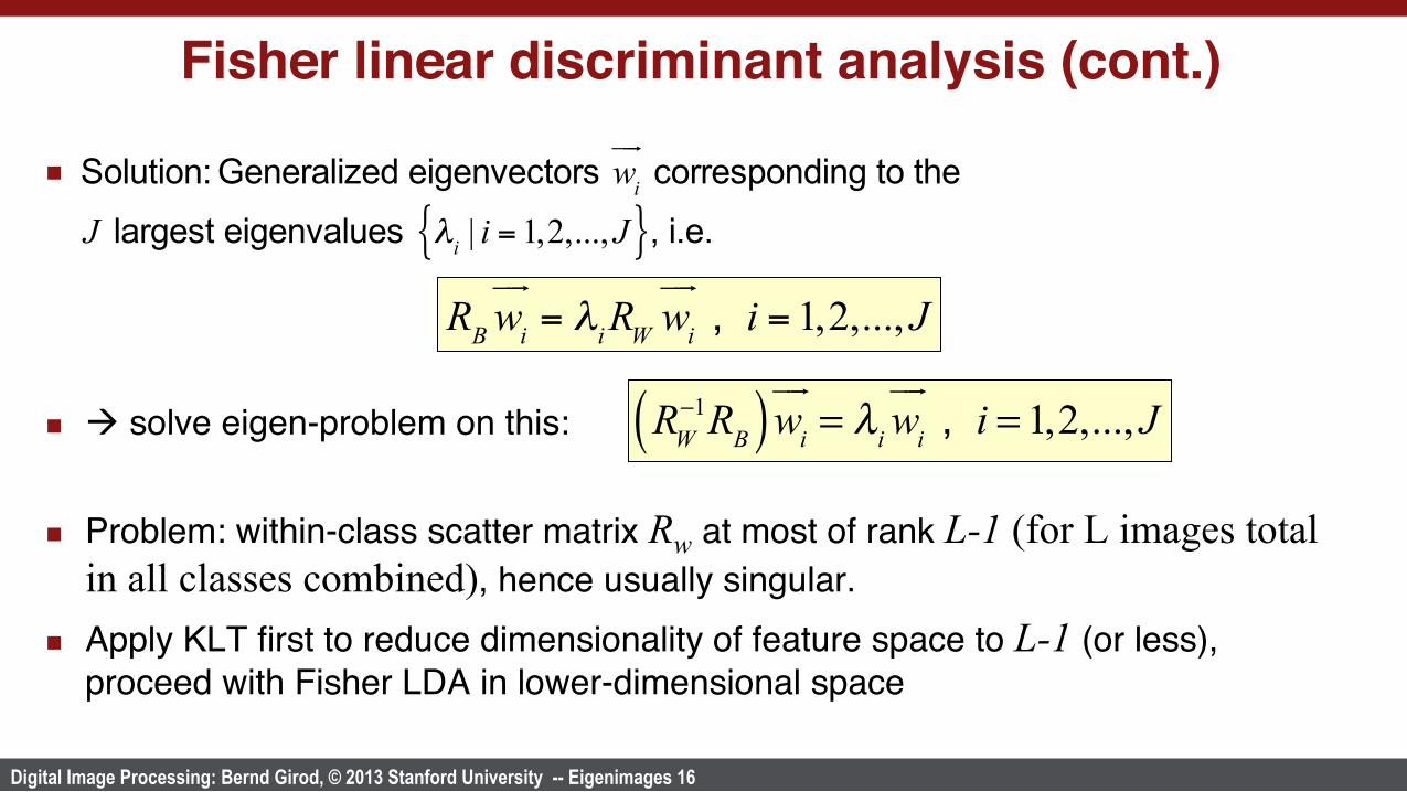
Fisher linear discriminant analysis (cont.)
n
n à solve eigen-problem on this:
n Problem: within-class scatter matrix Rw at most of rank L-1 (for L images total in all classes combined), hence usually singular.
n Apply KLT first to reduce dimensionality of feature space to L-1 (or less),proceed with Fisher LDA in lower-dimensional space
Solution: Generalized eigenvectors wi
!"! corresponding to the
J largest eigenvalues λi | i = 1,2,..., J{ }, i.e.
RB wi
!"!= λi RW wi
!"! , i = 1,2,..., J
RW
−1RB( )wi
!"!= λi wi
!"! , i = 1,2,..., J

Digital Image Processing: Bernd Girod, © 2013 Stanford University -- Eigenimages 17
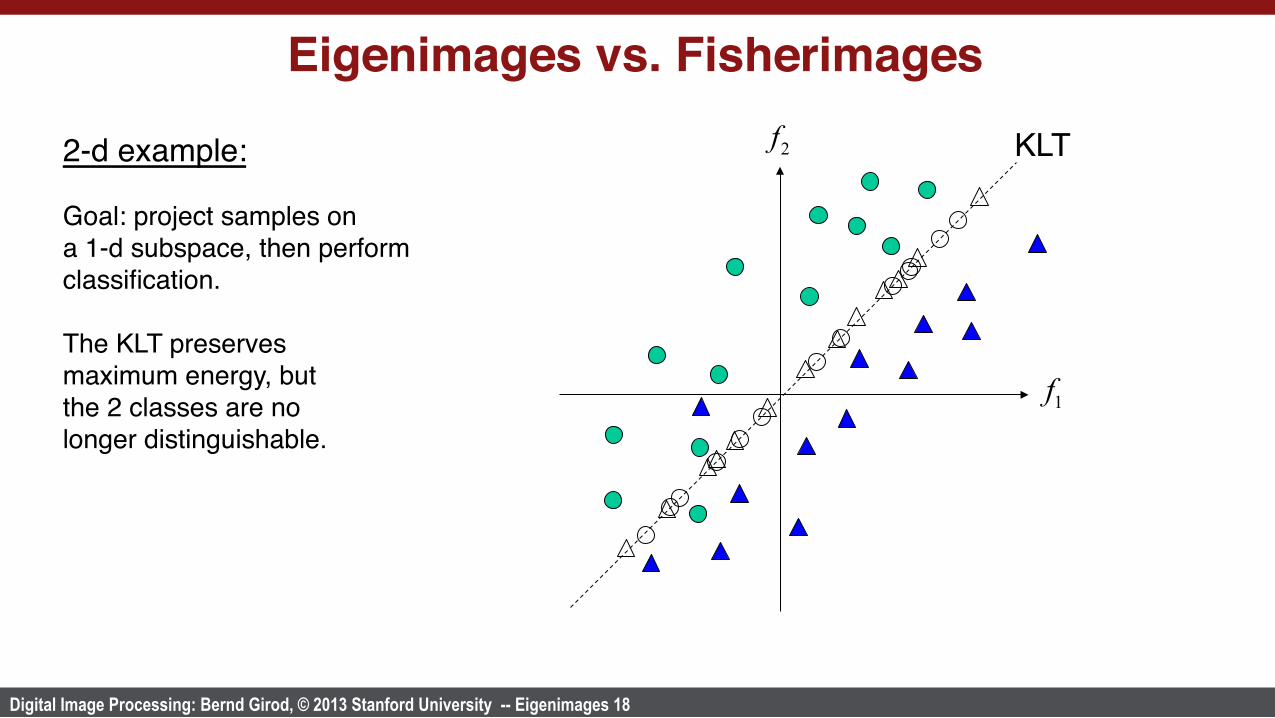
Eigenimages vs. Fisherimages
1f
2f2-d example:
Goal: project samples ona 1-d subspace, then performclassification.
Digital Image Processing: Bernd Girod, © 2013 Stanford University -- Eigenimages 18
Eigenimages vs. Fisherimages
1f
2f KLT2-d example:
Goal: project samples ona 1-d subspace, then performclassification.
The KLT preserves maximum energy, butthe 2 classes are no longer distinguishable.

Digital Image Processing: Bernd Girod, © 2013 Stanford University -- Eigenimages 19
Eigenimages vs. Fisherimages
2-d example:
Goal: project samples ona 1-d subspace, then performclassification.
The KLT preserves maximum energy, butthe 2 classes are no longer distinguishable.Fisher LDA separates the classes by choosing a better 1-d subspace.
1f
2f KLT
Fisher LDA

Digital Image Processing: Bernd Girod, © 2013 Stanford University -- Eigenimages 20
Fisherimages and varying iIllumination Differences due to varying illumination can be much larger than differences among faces!

Digital Image Processing: Bernd Girod, © 2013 Stanford University -- Eigenimages 21
Fisherimages and varying iIllumination
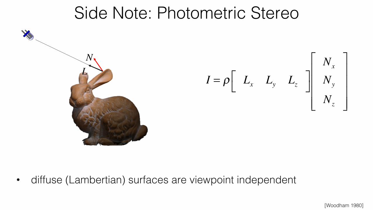
n All images of same Lambertian surface with differentillumination (without shadows) lie in a 3d linear subspace
n Single point source at infinity
n Superposition of arbitrary number of point sources at infinitystill in same 3d linear subspace, due to linear superposition of each contribution to image
n Fisherimages can eliminate within-class scatter
surfacenormal
!n !llight sourcedirection
f x, y( ) = a x, y( )
!l T !n x, y( )( )L
Light source intensity
Surface albedo

Side Note: Photometric Stereo!
I = ρL ⋅N
• diffuse (Lambertian) surfaces are viewpoint independent!
albedo!(constant)!
observed intensity!
normalized lighting direction!
normalized surface normal!
LN
[Woodham 1980]!
Side Note: Photometric Stereo!
• diffuse (Lambertian) surfaces are viewpoint independent!
LN
I = ρ Lx Ly Lz⎡⎣
⎤⎦
Nx
Ny
Nz
⎡
⎣
⎢⎢⎢⎢
⎤
⎦
⎥⎥⎥⎥
[Woodham 1980]!

Side Note: Photometric Stereo!
L 1( ) I (1)
I (2)
I (3)
⎡
⎣
⎢⎢⎢
⎤
⎦
⎥⎥⎥= ρ
Lx(1) Ly
(1) Lz(1)
Lx(2) Ly
(2) Lz(2)
Lx(3) Ly
(3) Lz(3)
⎡
⎣
⎢⎢⎢⎢
⎤
⎦
⎥⎥⎥⎥
Nx
Ny
Nz
⎡
⎣
⎢⎢⎢⎢
⎤
⎦
⎥⎥⎥⎥
• diffuse (Lambertian) surfaces are viewpoint independent!• assume albedo is constant, invert matrix!
L 2( )
L 3( )N
N = L−1I
LI =!=!
[Woodham 1980]!
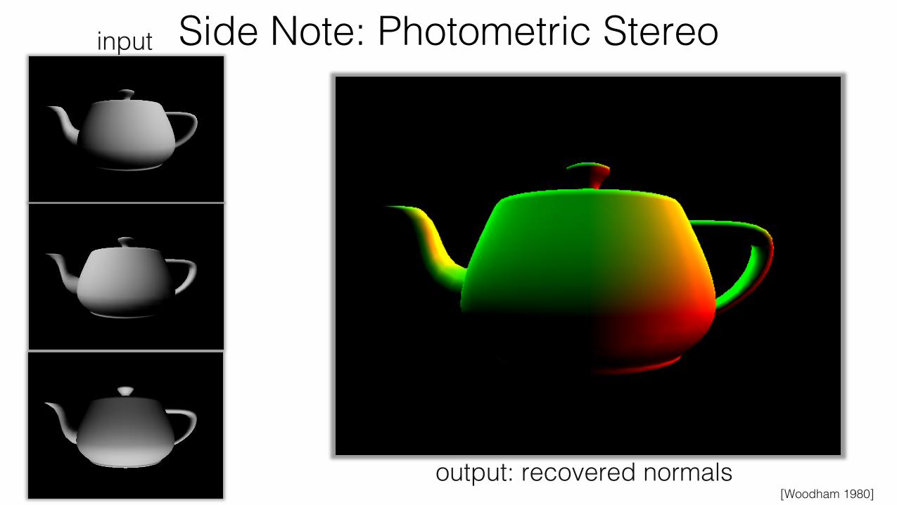
Side Note: Photometric Stereo!
[Woodham 1980]!output: recovered normals!
input!

Digital Image Processing: Bernd Girod, © 2013 Stanford University -- Eigenimages 26
Fisherface trained to recognize gender
Mean image Female mean Male meanµ! 1µ
!2µ!
Fisherface
Female face samples
Male face samples
Digital Image Processing: Bernd Girod, © 2013 Stanford University -- Eigenimages 27
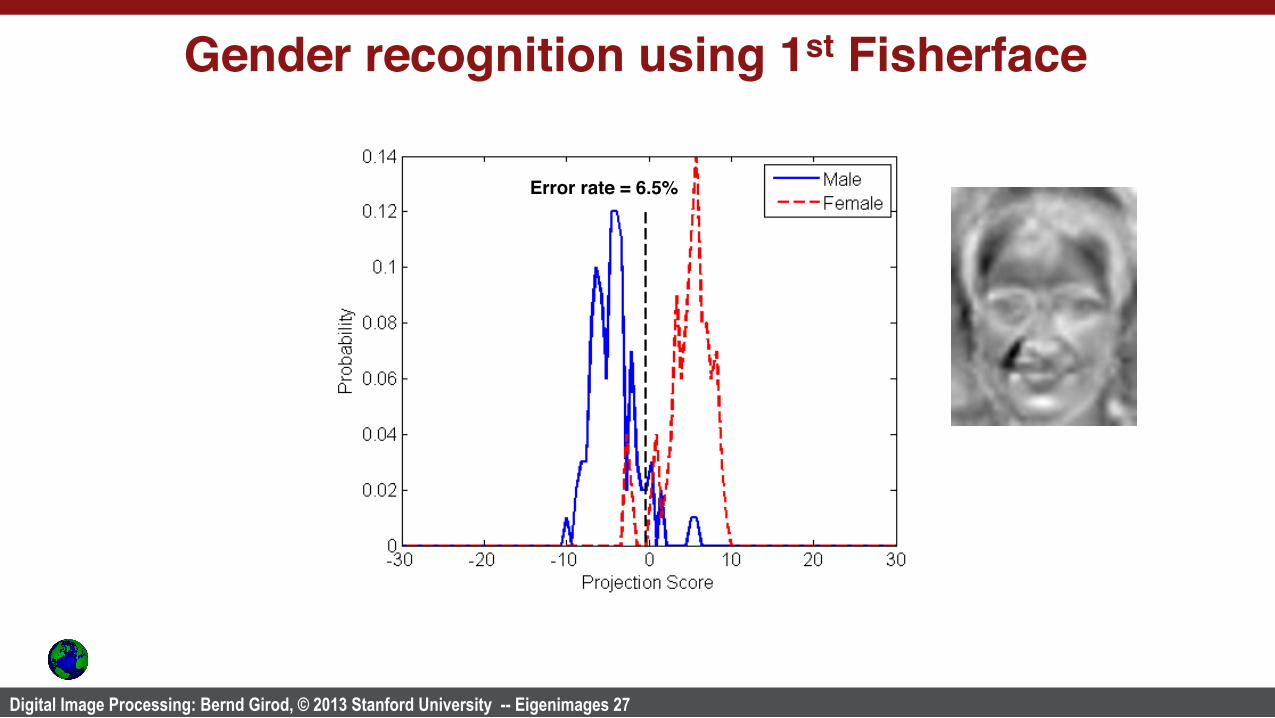
Gender recognition using 1st Fisherface
Error rate = 6.5%

Digital Image Processing: Bernd Girod, © 2013 Stanford University -- Eigenimages 28
Gender recognition using 1st eigenface
Error rate = 19.0%
Digital Image Processing: Bernd Girod, © 2013 Stanford University -- Eigenimages 29
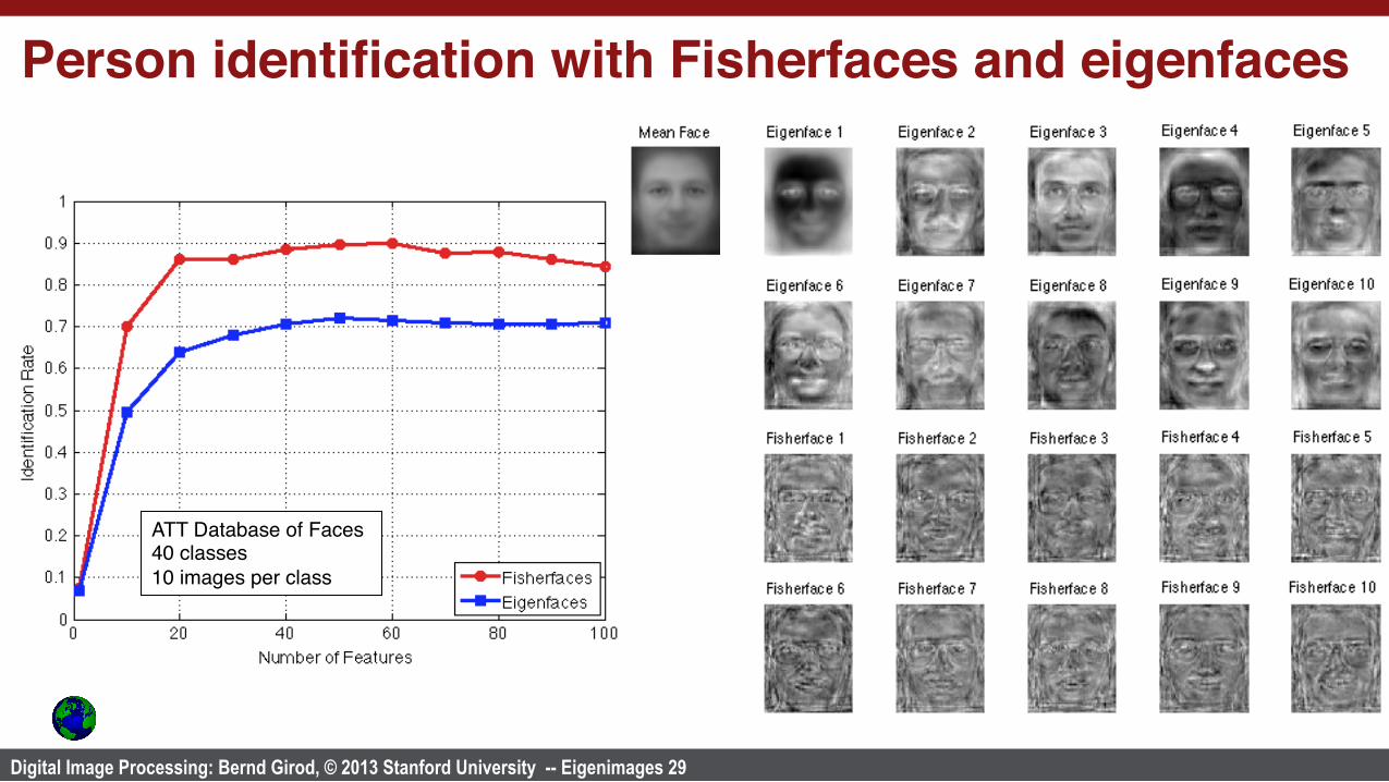
Person identification with Fisherfaces and eigenfaces
ATT Database of Faces40 classes10 images per class


![[Jean-Baptiste FIOT] Eigenfaces for Recognition](https://img.pdfslide.net/doc/110x75/55cf92f9550346f57b9acae0/jean-baptiste-fiot-eigenfaces-for-recognition.jpg)