Eigenvalue inclusion regions from inverses of

shifted matrices

Michiel E. Hochstenbach a, David A. Singer b, Paul F. Zachlin b

a Department of Mathematics and Computer Science, TU Eindhoven, PO Box513, NL-5600 MB Eindhoven, The Netherlands. The work of this author was

supported in part by NSF grant DMS-0405387.bDepartment of Mathematics, Case Western Reserve University, 10900 Euclid

Avenue, Cleveland, OH 44106-7058, USA

Abstract

We consider eigenvalue inclusion regions based on the field of values, pseudospectra,Gershgorin region, and Brauer region of the inverse of a shifted matrix. A familyof these inclusion regions is derived by varying the shift. We study several proper-ties, one of which is that the intersection of a family is exactly the spectrum. Thenumerical approximation of the inclusion sets for large matrices is also examined.

Key words: Harmonic Rayleigh–Ritz, inclusion regions, exclusion regions,inclusion curves, exclusion curves, field of values, numerical range, large sparsematrix, Gershgorin regions, ovals of Cassini, Brauer regions, pseudospectra,subspace methods, Arnoldi

1 Introduction

Let A be a nonsingular n× n matrix with spectrum Λ(A) and field of values(or numerical range)

W (A) ={

x∗Ax

x∗x: x ∈ Cn \{0}

}.

Email addresses: m.e.hochstenbach tue.nl (Michiel E. Hochstenbach),david.singer case.edu (David A. Singer), paul.zachlin case.edu(Paul F. Zachlin).

Preprint submitted to Elsevier 20 June 2008

While it is well known that Λ(A) ⊆ W (A), it was noted in [10, 11] that wealso have

Λ(A) ⊆ W (A) ∩ 1

W (A−1). (1)

Here 1/W (A−1) is interpreted as the set

1

W (A−1):={

1

z: z ∈ W (A−1)

}.

In this paper we will, inspired by the harmonic Rayleigh–Ritz technique, con-sider generalizations of (1) and study their properties. Section 2 briefly reviewsharmonic the Rayleigh–Ritz approach, mentions some new results, and givesan idea why this technique may be exploited for spectral inclusion regions. InSection 3 eigenvalue inclusion regions based on the field of values of the inverseof a shifted version of the matrix are introduced. We characterize the spec-trum of a matrix in a new way as the intersection of a family of these inclusionregions. Sections 4 and 5 focus on inclusion regions derived from Gershgorinand Brauer regions, and pseudospectra of shift-and-invert matrices. The prac-tical subspace approximation of some of the introduced sets for large matricesis considered in Section 6. We give a few examples of the techniques and apractical algorithm in Section 7 and end with some conclusions in Section 8.For other results on inclusion regions see, e.g., [1].

2 Harmonic Rayleigh–Ritz and fields of values

The sets W (A) and 1/W (A−1) have close connections with eigenvalue approx-imations from subspaces. Indeed, W (A) can be seen as the set of all possibleRitz values from a one-dimensional subspace; see, e.g., [15] or also [5]. As wasnoted in [5], in view of

{x∗x

x∗A−1x: x 6= 0

}=

{y∗A∗Ay

y∗A∗y: y 6= 0

}, (2)

the set 1/W (A−1) is exactly the set of all possible harmonic Ritz valuesdetermined by the harmonic Rayleigh–Ritz method with respect to targetτ = 0 from a one-dimensional subspace. After a brief review of the harmonicRayleigh–Ritz approach, we will point out a generalization of this statementin Proposition 1 below.

The harmonic Rayleigh–Ritz technique [12–14] was introduced to better ap-proximate interior eigenvalues using subspace methods near a given targetτ ∈ C. Consider the standard eigenvalue problem Ax = λx, and let U be a

2

low dimensional search space for an eigenvector x with associated search ma-trix U of which the columns form an orthonormal basis for U . We are interestedin an approximation (λ, x) ≈ (θ, u) with u ∈ U . Instead of the Galerkin con-dition Au − θu ⊥ U of the standard Rayleigh–Ritz extraction, the harmonicRayleigh–Ritz extraction with target τ imposes the Galerkin condition

Au− θu ⊥ (A− τI)U . (3)

This implies that a harmonic Ritz value θ satisfies

θ =u∗(A− τI)∗Au

u∗(A− τI)∗u,

where u is a harmonic Ritz vector.

As a generalization of (2) we have the following result. Note that in thisproposition and throughout this paper addition and division are interpretedelementwise: for a set S, we define

1

S+ τ :=

{1

z+ τ : z ∈ S

}.

Proposition 1

1

W ((A− τI)−1)+ τ =

{y∗(A− τI)∗Ay

y∗(A− τI)∗y: y 6= 0

}.

Proof: This follows easily from the equality{x∗x

x∗(A− τI)−1x+ τ : x 6= 0

}=

{y∗(A− τI)∗(A− τI)y

y∗(A− τI)∗y+ τ : y 6= 0

}.

2

Therefore, the set of all possible harmonic Ritz values with respect to targetτ is the reciprocal of W ((A− τI)−1) shifted by τ .

An important property of harmonic Ritz values θ with respect to target τ isthat they tend to stay away from this τ , which we shall study more closelyin Section 6 (Proposition 14). Because of this property harmonic Ritz valuesare exploited in several situations. For instance, the GMRES method implic-itly uses harmonic Ritz values for interpolation of the function f(z) = z−1

resulting from linear systems Ax = b. Also, these values have found their wayinto the approximation of problems involving more general matrix functionsf(A) b where one would like to avoid a specific target. One example is the signfunction which has a discontinuity in z = 0 [4, 16]. In this paper we will usesets as the one in Proposition 1 for eigenvalue inclusion regions.

3

A new interesting observation is the following. If we write η = τ−1 then (3)is equivalent to Au − θu ⊥ (ηA − I)U . If we take the limit |τ | → ∞ or,equivalently, η → 0, we see that the standard Rayleigh–Ritz method can beviewed as the harmonic Rayleigh–Ritz method with target at infinity; see alsothe related Theorem 5 in the next section.

3 Eigenvalue inclusion regions from the field of values of inversesof shifted matrices

Let τ be a complex number not equal to an eigenvalue of A. A crucial obser-vation that we will use is that

Λ(A) =1

Λ((A− τI)−1)+ τ.

Since Λ((A− τI)−1) ⊆ W ((A− τI)−1), we know that for every τ 6∈ Λ(A) thespectrum Λ(A) is included in the set

1

W ((A− τI)−1)+ τ (4)

and therefore

Λ(A) ⊆⋂

τ∈C \Λ(A)

1

W ((A− τI)−1)+ τ. (5)

The following theorem shows that this inclusion is in fact an equality.

Theorem 2

Λ(A) =⋂

τ∈C \Λ(A)

1

W ((A− τI)−1)+ τ.

Proof: Suppose we have z ∈ C \Λ(A). We still need to show that

z /∈ 1

W ((A− τI)−1)+ τ

for some choice of τ ∈ C \Λ(A). We see this is true by letting τ = z, becauseotherwise we would have

0 ∈ 1

W ((A− zI)−1),

which contradicts the fact that W ((A− zI)−1) is a bounded set. 2

4

From the proof of Theorem 2 we already see that the set (4) never includes τitself. Indeed, we have the following proposition.

Proposition 3 If ‖ · ‖ is any subordinate norm, then

dist

(τ,

1

W ((A− τI)−1)+ τ

)≥ ‖(A− τI)−1‖−1.

Proof: This follows from the fact that the set W ((A−τI)−1) is inside the diskaround zero with radius ‖(A − τI)−1‖. Note that for the two-norm we have‖(A − τI)−1‖−1

2 = σmin(A − τI), where σmin indicates the minimal singularvalue. 2

This implies that, once we already have an eigenvalue inclusion region, we canexclude a neighborhood of any τ 6∈ Λ(A), and thereby improve the inclusionregion, by taking the intersection of the region with 1/W ((A− τI)−1) + τ .

Moreover, inspecting the proof of Theorem 2, we observe that the only prop-erty of the field of values that we use is the fact that it is a bounded set thatcontains the eigenvalues of the matrix. Realizing this, we immediately arriveat the following theorem.

Theorem 4 Let G be a set-valued function from the set of complex n × nmatrices to subsets of C, such that for any A the set G(A) is bounded andcontains Λ(A). Then

Λ(A) =⋂

τ∈C \Λ(A)

1

G((A− τI)−1)+ τ.

This result will be used later on in the paper.

We now study properties of the set (4) for varying τ . The next, somewhatsurprising, result shows that if |τ | → ∞, the inclusion region (4) converges toW (A).

Theorem 5

lim|τ |→∞

(1

W ((A− τI)−1)+ τ

)= W (A).

Proof: With Proposition 1 and η = τ−1, the result follows from

5

{lim|τ |→∞

y∗(A− τI)∗Ay

y∗(A− τI)∗y: y 6= 0

}=

{limη→0

y∗(ηA− I)∗Ay

y∗(ηA− I)∗y: y 6= 0

}

=

{y∗Ay

y∗y: y 6= 0

}= W (A).

2

We remark that in the case that A is a normal matrix this theorem has thefollowing geometric interpretation. Since the field of values is unitarily invari-ant, we may assume that A is a diagonal matrix and hence (A − τI)−1 =diag((aii − τ)−1). The field of values of a normal matrix is the convex hull ofits eigenvalues [6, p. 11], which in this case are its diagonal entries, and thisimplies that (4) is a circular-arc polygon with vertices at a11, . . . , ann. (By acircular-arc polygon we mean a closed set in the complex plane with boundaryconsisting of up to n circular arcs; here, the intersection of any two of thesearcs is one of the eigenvalues a11, . . . , ann.) By choosing τ large enough thecircular arcs connecting the eigenvalues get arbitrarily close to the straightline segments connecting the eigenvalues as we can see as follows. Supposethat L is a line through (aii − τ)−1 and (ajj − τ)−1. Then, 1

L+ τ (interpreted

elementwise as before) is the circle passing through aii, ajj, and τ . Noticethat as |τ | → ∞, the radius of this circle also approaches infinity, and so thecircular arc approaches the straight line through aii and ajj.

Kippenhahn [8] (see also [19]) showed that the field of values of an n×n matrixis the convex hull of an algebraic curve of class n called the boundary gener-ating curve and that the foci of this curve are the eigenvalues of the matrix.(The class of a curve is the degree of the polynomial P (u, v) whose zeroes givethe lines ux+vy = 1 which are tangent to the curve. We can also characterizethe class of a curve as the number of tangents—real or imaginary—that canbe drawn from a point to the curve. The notion of algebraic foci generalizesthe familiar definition for conics to algebraic curves of arbitrary degree. See,for example, [2, Section 3] for a recent discussion.) Taking the reciprocal ofthe boundary generating curve of W ((A− τI)−1) and adding τ gives anotheralgebraic curve such that the eigenvalues of A are still foci of the curve. There-fore in the special case where the boundary of the field of values of the matrixA is the same as its boundary generating curve, the entire family of curvesformed by the boundaries of the sets (4) is confocal, i.e., every curve in thisfamily has the same foci.

Theorems 2 and 5 imply that the inclusion set (1) is actually a rather restrictedspectral inclusion set where in (5) we only take the intersection of the sets (4)for τ = 0 and τ = ∞. Moreover, apparently the inclusion set W (A) can be“simulated” by the set (4) for |τ | → ∞.

6

We observe that although W ((A − τI)−1) is a bounded set, the set (4) mayor may not be bounded, depending on whether or not the origin is con-tained in W ((A − τI)−1). If a neighborhood of 0 is inside W (A − τI) then1/W ((A − τI)−1) + τ is an unbounded eigenvalue inclusion region with abounded complement. For this reason, it may be more convenient to think ofthe bounded complement of 1/W ((A− τI)−1) + τ as an eigenvalue exclusionregion. We will illustrate this with an example in Figure 1. It is suggestive hereto speak of the boundary of (4) as an inclusion or exclusion curve, dependingon whether it is the boundary of a bounded inclusion or exclusion region.

We will illustrate the results with the 300×300 randcolu matrix of Matlab’sgallery. In Figure 1, two targets are taken that are inside the field of values,so that the set 1/W ((A − τI)−1) + τ is an unbounded inclusion region; itscomplement can be seen as a bounded exclusion region.

−2 −1 0 1 2 3−1.5

−1

−0.5

0

0.5

1

1.5

Real

Imag

−2 −1 0 1 2 3−1.5

−1

−0.5

0

0.5

1

1.5

Real

Imag

(a) (b)

Fig. 1. (a) Spectrum, W (A) (solid) and 1/W ((A− τI)−1)+ τ (dot) of the 300×300randcolu matrix for the shift τ = 1.2, also indicated by an asterisk. The dottedline is the boundary of the unbounded inclusion region 1/W ((A − τI)−1) + τ andits bounded complement which forms an exclusion region. (b) Idem but now forτ = 1.3, which is still inside W (A). As a consequence, the inclusion region is stillunbounded.

For Figure 2, two targets are taken that are outside the field of values, so thatthe set 1/W ((A− τI)−1) + τ is a bounded inclusion region. In Figure 2(b) westart to see convergence to W (A).

Since the field of values contains the spectrum, a neighborhood of the originwill often be in W (A − τI) if we choose τ sufficiently close to an eigenvalue,in which case (4) is unbounded. (Note that this is not always the case, forinstance if τ is located close to an eigenvalue but just outside the field ofvalues of a normal matrix.) On the other hand, if |τ | is large enough, thenaccording to Theorem 5 the set (4) is a bounded inclusion region.

7

−2 −1 0 1 2 3−1.5

−1

−0.5

0

0.5

1

1.5

Real

Imag

−2 −1 0 1 2 3−1.5

−1

−0.5

0

0.5

1

1.5

Real

Imag

(a) (b)

Fig. 2. (a) Same as in Figure 1 but now for shift τ = 1.33, which is outside W (A),which results in a bounded inclusion region. (b) Idem, but now for τ = 1.5.

Let us now consider the transition case, in which τ is such that the origin is onthe boundary of W ((A− τI)−1). This means that 1/W ((A− τI)−1) + τ is anunbounded inclusion region while the complement is also unbounded. In thiscase the boundary of (4) passes through infinity, and is neither an inclusioncurve nor an exclusion curve, so in this case we will call the boundary of (4) atransition curve of A. The next result deals with the question of which valuesof τ give rise to a transition curve.

Theorem 6 Let τ 6∈ Λ(A). The boundary of (4) is a transition curve of A ifand only if τ is on the boundary of W (A).

Proof: Since τ is not an eigenvalue and

W ((A− τI)−1) =

{x∗(A− τI)∗x

x∗(A− τI)∗(A− τI) x: x 6= 0

}

we have that 0 ∈ W ((A − τI)−1) if and only if there exists a nonzero x suchthat x∗(A− τI)∗x = 0, which means that τ ∈ W (A). 2

In the next section, we will generalize the above results by substituting for thefield of values another well-known eigenvalue inclusion region, the Gershgorinregion. Before proceeding, however, we make one final geometric observationfor the case of the field of values.

Suppose ξ is an algebraic curve which is the boundary of the set (4), and thatthe target τ is in the interior of the field of values so that ξ is an exclusion curve.Such a curve is known to have interesting analytic properties; in particular,we know from [9, Thm. 1.1] that if ξ is an eigenvalue exclusion curve, then itis the boundary of a quadrature domain D. That is, there exist finitely manypoints zk = xk + iyk ∈ D and constants γ1, . . . , γr, such that the following

8

quadrature identity holds for functions h(x, y) which are harmonic on theclosure of D:

∫∫D h(x, y)dxdy =

∑rk=1 γkh(xk, yk). In the simplest nontrivial

case, where A is a 2 × 2 matrix, the boundaries of the sets (4) are confocalellipses when they are inclusion curves, and inverted ellipses when they areexclusion curves. The inverted ellipse, also known as Neumann’s quadraturedomain, is the earliest historical example of a curve satisfying a (two-point)quadrature identity. Note, incidentally, that the two points z1 and z2 in thisquadrature identity are not the eigenvalues of A; see [3] for more information.

4 Eigenvalue inclusion regions from the Gershgorin and Brauerregions of inverses of shifted matrices

The union of Gershgorin disks is another type of famous eigenvalue inclusionregion. Richard Varga has proved many beautiful Gershgorin results, culmi-nating in the book [17]. In this section, we show that similar results to someof those derived for the field of values in the previous section can be obtainedfor Gershgorin regions.

With 1 ≤ i ≤ n and

ri(A) :=∑j 6=i

|aij|,

recall that

Γi(A) := {z ∈ C : |z − aii| ≤ ri(A)}

is the ith Gershgorin disk of A. Now define the Gershgorin region to be theunion of the Gershgorin disks, i.e.,

Γ(A) :=⋃

1≤i≤n

Γi(A).

It is well known that the Gershgorin region is an eigenvalue inclusion region:since each eigenvalue λ is element of at least one disk, we have λ ∈ Γ(A) (see,for example, [17]).

Now for a shifted matrix A we consider the Gershgorin region of the inverse:we will study the sets

1

Γi((A− τI)−1)+ τ (6)

and

1

Γ((A− τI)−1)+ τ. (7)

9

Similar to Theorem 2 for the field of values, we have the following result.

Theorem 7

Λ(A) =⋂

τ∈C \Λ(A)

1

Γ((A− τI)−1)+ τ.

Proof: This follows immediately from Theorem 4. 2

Analogous to Theorem 5, we have the following result.

Theorem 8

lim|τ |→∞

(1

Γi((A− τI)−1)+ τ

)= Γi(A)

and, consequently,

lim|τ |→∞

(1

Γ((A− τI)−1)+ τ

)= Γ(A).

Proof: The set (6) consists of exactly the z for which∣∣∣∣ 1

z − τ− ((A− τI)−1)ii

∣∣∣∣ ≤∑i6=j

|((A− τI)−1)ij|.

Write η = τ−1, then we consider the situation η → 0. Since (A − τI)−1 =η (ηA− I)−1 the inequality becomes∣∣∣∣ τ

z − τ− ((ηA− I)−1)ii

∣∣∣∣ ≤∑i6=j

|((ηA− I)−1)ij|

or ∣∣∣∣∣ 1

ηz − 1− ((ηA− I)−1)ii

∣∣∣∣∣ ≤∑i6=j

|((ηA− I)−1)ij|.

Expanding in Taylor series we get∣∣∣(I + ηA +O(η2))ii − (1 + ηz +O(η2))∣∣∣ ≤∑

i6=j

|(I + ηA +O(η2))ij|.

Since Iii = 1 and Iij = 0 for j 6= i, we may write∣∣∣(ηA +O(η2))ii − (ηz +O(η2))∣∣∣ ≤∑

i6=j

|(ηA +O(η2))ij|.

10

This yields

|(aii − z +O(η))| ≤∑i6=j

|(aij +O(η))|,

so that in the limit η → 0 we get

|z − aii| ≤∑i6=j

|aij|.

The second statement of the theorem follows straightforwardly. 2

We note that another proof appeared in the Ph.D. thesis of the third author[18]. Since the reciprocal of a circle is a circle (or line), the boundary of eachof the sets (6) is a circle (or line). When |τ | is large enough, we know from thelast theorem that (6) is a disk converging to Γi(A), so that for large valuesof τ the union of the sets (6) is an eigenvalue inclusion region. The conceptof transition curves of the previous subsection does not carry over in a directmanner to the Gershgorin region since this set is a union of n disks, eachcontaining at least one eigenvalue; in general there will not be a τ so that alln sets are unbounded.

There are several generalizations of the Gershgorin region that yield othereigenvalue inclusion regions. We next consider the arguably best-known gen-eralization, the Brauer region. The region

Ki,j(A) := {z ∈ C : |z − aii| · |z − ajj| ≤ ri(A) · rj(A)}

is called the (i, j)-th Brauer Cassini oval of A. The Brauer region is definedto be the union of the Brauer Cassini ovals, i.e.,

K(A) :=⋃i6=j

Ki,j(A).

The Brauer region is at least as good an eigenvalue inclusion region as theGershgorin region: Λ(A) ⊆ K(A) ⊆ Γ(A); see, for example, [17].

By once again applying Theorem 4 we arrive at another characterization ofthe spectrum.

Theorem 9

Λ(A) =⋂

τ /∈Λ(A)

1

K((A− τI)−1)+ τ.

We also get an analogue of Theorem 8, which can be proven in an almostidentical way.

11

Theorem 10

lim|τ |→∞

(1

Ki,j((A− τI)−1)+ τ

)= Ki,j(A)

and, consequently,

lim|τ |→∞

(1

K((A− τI)−1)+ τ

)= K(A).

Similar to Proposition 3, the sets 1/Γ((A− τI)−1) and 1/K((A− τI)−1) avoidτ , as the following result shows.

Proposition 11

dist

(τ,

1

K((A− τI)−1)+ τ

)≥ dist

(τ,

1

Γ((A− τI)−1)+ τ

)≥ ‖(A−τI)−1‖−1

∞ .

Proof: This follows from K((A − τI)−1) ⊆ Γ((A − τI)−1) and the fact thatfor all z ∈ Γ((A− τI)−1) we have |z| ≤ ‖(A− τI)−1‖∞. 2

We believe that the techniques employed so far may also be useful in study-ing other generalizations of the Gershgorin region (see [17]), but rather thanproceed in this direction, we turn now to pseudospectra.

5 Eigenvalue inclusion regions from pseudospectra of inverses ofshifted matrices

The ε-pseudospectra of A, defined by

Λε(A) = {z : σmin(A− zI) ≤ ε}

are often studied to better understand the behavior of nonnormal matrices;see [15] for a recent overview.

By applying Theorem 4 we have immediately the following result.

Theorem 12

Λ(A) =⋂

τ /∈Λ(A)

1

Λε((A− τI)−1)+ τ.

Instead of an exact analogue of Theorem 5, we get the following result.

12

Theorem 13

limτ→∞

1

Λ ε|τ |2

((A− τI)−1)+ τ

= Λε(A).

Proof: The set

1

Λ ε|τ |2

((A− τI)−1)+ τ

consists of the z for which

σmin

(1

z − τI − (A− τI)−1

)≤ ε

|τ |2.

Again with η = τ−1 we get

σmin

(η

ηz − 1I − η (ηA− I)−1

)≤ ε |η|2

Expansion in Taylor series yields

σmin

(η(I + ηA +O(η2))− η(1 + ηz +O(η2)) I

)≤ ε |η|2

which means

|η|2 σmin(A− zI +O(η)) ≤ ε |η|2.

For η → 0 this yields Λε(A). 2

6 Subspace approximations for large matrices

In this and the following section we will show that the obtained results yieldpractical methods to approximate inclusion regions for large matrices. Sincethe computation of the inverse of a (shifted) large matrix will often be pro-hibitively expensive, we will consider approaches to numerically approximatethe sets (4) and (7) using subspace methods. This section studies the case forone shift and partly contains an extension of the methods of [5] for shiftedmatrices. We will use the approximations in Section 7 for a method giving anapproximate eigenvalue inclusion region using several suitably chosen shifts.

As already stated in Section 2, an important property of harmonic Ritz valuesθ with respect to target τ is that they tend to stay away from this τ . Although

13

this behavior is known from practical situations, we are not aware of any con-crete results showing this. The next proposition gives a result in this direction.As in Section 2, let U be a search space with associated matrix U of which thecolumns form an orthonormal basis for U . We make the natural assumptionthat (A − τI) U is of full rank; if this is not the case, τ is an eigenvalue andits corresponding eigenvector is in the space U—a fortunate event.

Proposition 14 Let (A− τI) U be of full rank, let U∗(A− τI)∗(A− τI) U =LL∗ be the Choleski decomposition (or matrix square root decomposition), andlet ‖ · ‖ be any subordinate norm. Then

|θ − τ | ≥ ‖L−1U∗(A− τI)∗UL−∗‖−1.

Proof: Since u ∈ U , we can write u = Uc for c ∈ Ck. Therefore, we have

(A− τI) u− (θ − τ) u ⊥ (A− τI)U

and, via

U∗(A− τI)∗(A− τI) Uc = (θ − τ) U∗(A− τI)∗Uc, (8)

this is equivalent to

L−1U∗(A− τI)∗ UL−∗d = (θ − τ)−1d,

where d = L∗c. The result now follows from the fact that the spectral radiusis bounded above by a subordinate matrix norm. 2

A field of values may be determined numerically by the method due to Johnson[7], but this may be expensive for large matrices. In this situation, Manteuffeland Starke [11] proposed to use the Arnoldi process to approximate bothW (A) and 1/W (A−1) as follows. Starting from an initial vector u1 with unitnorm, let

AUk = UkHk + hk+1,kuk+1e∗k = Uk+1Hk,

be the Arnoldi decomposition after k steps, where the columns of Uk forman orthonormal basis for the Krylov space Uk with u1 as its first column,Hk is an upper Hessenberg matrix, ek is the kth canonical basis vector, and

Hk =

[Hk

hk+1,ke∗k

]is a (k + 1)× k Hessenberg matrix with an extra row.

In [11], W (A) is approximated by

W (A) ⊇ W (U∗kAUk) = W (Hk). (9)

14

For the approximation of 1/W (A−1), we first introduce the reduced QR-decomposition Hk = QkRk, so that AUkR

−1k = Uk+1HkR

−1k = Uk+1Qk has

orthonormal columns. Then W (A−1) is approximated in [11] as follows:

W (A−1) ⊇ W (R−∗k U∗

kA∗A−1AUkR−1k ) = W (R−∗

k H∗kR−1

k ). (10)

(In fact, this is the derivation in [5]; [11] used a different one.)

As noted in [5,11], while approximation (9) for W (A) is often very reasonable,approximation (10) for W (A−1) is frequently disappointing. In practical sit-uations, approximation (10) may not contain the eigenvalues of A−1, so that1/W (A−1) does not contain Λ(A). This implies that this numerical approxi-mation of (1) does not contain the spectrum.

For this reason, in [5] the approximation

W (A−1) ⊇ W (U∗kA−1Uk) ≈ W (H−1

k )

was introduced which no longer guarantees a strict inclusion but in practicemay be a much better approximation to W (A−1).

We now discuss the numerical approximation of W ((A− τI)−1) for large ma-trices using subspace techniques. We present two alternative approximationswhich are (relatively straightforward) extensions of the approaches in [5].

For the first approximation, let Ik be the k×k-identity with an extra (k+1)stzero row. With the reduced QR-decomposition Hk − τIk = QkRk, the matrix(A− τI) UkR

−1k has orthonormal columns, and we therefore have

W ((A− τI)−1)⊇W (R−∗k U∗

k (A− τI)∗(A− τI)−1(A− τI) UkR−1k )

(11)= W (R−∗

k (Hk − τIk)∗R−1

k ).

Recall from (8) that the eigenvalues of

(U∗k (A− τI)∗Uk)

−1U∗k (A− τI)∗(A− τI) Uk = (Hk − τIk)

−∗R∗kRk

are the harmonic Ritz values shifted by −τ of A with respect to search spaceUk and shift τ . Since the eigenvalues of R−∗

k (Hk − τIk)∗R−1

k are identical tothose of R−1

k R−∗k (Hk − τIk)

∗, we conclude that after k steps we know that (4)contains the convex hull of the harmonic Ritz values with respect to shift τ .

A second approach to approximate W ((A− τI)−1) is to discard the last termin the expression

U∗k (A− τI)−1Uk = (Hk − τI)−1 − hk+1,kU

∗k (A− τI)−1uk+1e

∗k(Hk − τI)−1.

15

and approximate

W ((A− τI)−1) ⊇ W (U∗k (A− τI)−1Uk) ≈ W ((Hk − τI)−1). (12)

This approximation is not an inclusion in general but may be satisfactoryprovided that ‖(A − τI)−1‖2 and ‖(H − τI)−1‖2 are not too large. Indeed,experiments in [5] indicate that (12) is often much more favorable than (11);we will use (12) in the next subsection.

Finally, to numerically approximate Γ((A− τI)−1) and K((A− τI)−1) usingthe Krylov subspace Uk, we can approximate (A− τI)−1 ≈ Uk(Hk − τI)−1U∗

k .The inspiration for this is the following. For arbitrary w ∈ Cn, v = (A−τI)−1wcan be approximated from the subspace Uk by

v ≈ vk = Ukc, w − (A− τI) vk ⊥ Uk,

so that vk = Ukc = Uk(H− τI)−1U∗kw. The elements ((A− τI)−1)ij that occur

in Γ((A− τI)−1) and K((A− τI)−1) can then be efficiently approximated by(e∗i Uk)((Hk−τI)−1(U∗

kej)). We will give examples of the mentioned approachesin the next section.

7 Numerical examples and an algorithm

Before we will propose an algorithm to get an inclusion region based on thefield of values, we first perform a number of experiments with the 1000×1000grcar matrix. In Figure 3(a) the spectrum (dots), the inclusion region W (A)(solid line), and the unbounded inclusion regions 1/W ((A−τI)−1)+τ (dottedline) are indicated for the targets τ = 0, and τ = ±i/2. The “repelling force” ofthe targets resulting in exclusion regions containing the targets—the boundedcomplements of the inclusion regions 1/W ((A−τI)−1)+τ—is clear. Note thatthe intersections of the four inclusion sets gives a much better inclusion regionthan Λ ⊆ W (A) alone, but also that the regions derived with the targetsτ = ±i/2 add little to the final result.

For Figure 3(b) we plot approximations to the inclusion regions (4) for severalvalues of τ : 0, ±i, 2 ± 2i, and 3. We generate a 10-dimensional Krylov spaceK(A, b) for a random vector b and take the approximation (12), which for τ = 0was found to be often better than (11) in [5]. We see for this example that aslong as τ is not too close to an eigenvalue, the approximation (12) is indeedan inclusion region. All bounded regions with dotted lines as boundaries areexclusion regions, being bounded complements of unbounded inclusion regions,except for the region corresponding to τ = 3, which is a bounded inclusionregion. Without further details, we mention that the approximations (11) with

16

−6 −4 −2 0 2 4−4

−3

−2

−1

0

1

2

3

4

Real

Imag

−8 −6 −4 −2 0 2 4 6−5

0

5

Real

Imag

(a) (b)

Fig. 3. (a) Spectrum, W (A) (solid) and 1/W ((A − τI)−1) + τ (dotted) of the1000 × 1000 grcar matrix and targets τ = 0, ±i/2. The targets are indicatedby dots. (b) The same but here the sets 1/W ((A − τI)−1) + τ (dot) are numeri-cally approximated by (12) using a 10-dimensional Krylov space. We use the targetsτ = 0, ±i, 2± 2i and 3.

the same targets were all “inclusion regions” of poor quality: they includednot all eigenvalues, or even none.

Now we come to the important question how to choose sensible targets τ ,given a matrix A. Since W (A) is an inclusion region, it is natural to take τ onor near to the boundary of the field of values to get more restrictive inclusionregions. We already have seen an example of this in Figure 3.

Based on this idea, we now develop an automatic procedure to get an (approx-imate) eigenvalue inclusion region from a low-dimensional Krylov space. Firstwe generate a low, k-dimensional Krylov space Kk(A, u1) for a starting vectoru1, yielding a Krylov relation AUk = UkHk + hk+1,kuk+1e

∗k. We approximate

W (A) by W (Hk), where, in turn, we approximate W (Hk) by m “angles” (thatis, by multiplying Hk by factors of the form e−iαj , j = 1, . . . ,m; see [7]). A lownumber m between, say, 8 and 32 often already gives excellent results. Thisprocess gives 2m points τj (every angle determines two points: a minimal andmaximal eigenvalue of a “rotated” matrix [7]) that are on the boundary ofW (Hk), inside W (A), and often also close to the boundary of W (A).

Given these points τj, j = 1, . . . , 2m, the sets 1/W ((A − τjI)−1) + τj areunbounded inclusion regions of which the bounded complements are exclusionregions since the τj are inside W (A) (see Section 3). Since W ((A− τjI)−1) iscomputationally expensive to determine, we approximate 1/W ((A−τjI)−1)+τj by the sets 1/W ((Hk−τjIk)

−1)+τj. We stress the fact that this is an efficientprocedure since we use the same low-dimensional Krylov space to approximateW (A) by W (Hk) and 1/W ((A− τjI)−1) + τj by 1/W ((Hk − τjIk)

−1) + τj. Asdiscussed in the previous section, these approximations are not guaranteed to

17

be true inclusion regions, but may be promising inclusion regions in practicalsituations. As a result, this procedure gives an approximate inclusion regionas the intersection of W (Hk) and

⋂j 1/W ((Hk − τjIk)

−1) + τj. In Algorithm 1we summarize the algorithm.

Algorithm 1 A method to determine an (approximate) inclusion region basedon fields of values and a Krylov space.

Input: A matrix A, starting vector u1, dimension of Krylov space k, andnumber of angles mOutput: An (approximate) spectral inclusion region

1: Compute the Krylov space Kk(A, u1)

with associated relation AUk = UkHk + hk+1,kuk+1e∗k

2: Approximate W (A) by W (Hk) using m angles, giving 2m points τj ∈ Cthat are inside and usually near the boundary of W (A)

for j = 1 : 2m

3: Approximate 1/W ((A− τjIn)−1) + τj by 1/W ((Hk − τjIk)−1) + τj

(using a low number of angles for W ((Hk − τjIk)−1))

end

4: The (approximate) spectral inclusion region is given by the intersection

of W (Hk) and⋂2m

j=1 1/W ((Hk − τjIk)−1) + τj

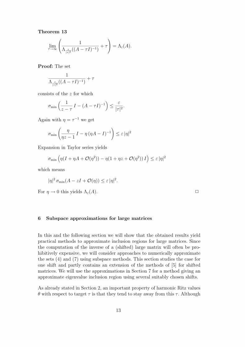
The results of Algorithm 1 for k = 10 (dimension of the Krylov subspace) andm = 8 (number of “angles” to approximate W (Hk)) are shown in Figure 4.Although there are many curves, the relevant region is the interior of the fieldof values, where the intersection with the inclusion sets 1/W ((Hk−τjI)−1)+τj

is seen to give a tighter eigenvalue inclusion region than W (Hk) alone.

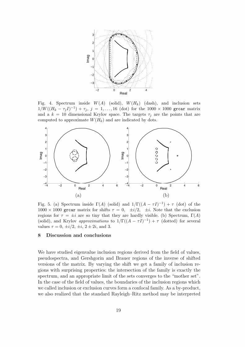
Finally, we perform some experiments with inclusion regions based on Ger-shgorin disks. In Figure 5(a) we take the same matrix; this time we plot thespectrum (dots), and the inclusion regions defined by the Gershgorin regionΓ(A) (solid line) and 1/Γ((A − τI)−1) + τ (dotted lines) for τ = 0, ±i/2,±i. We see that the plotted inclusion regions based on the Gershgorin regionsseem less promising than those based on the field of values.

For Figure 5(b) we plot approximations to the inclusion regions (7) for τ = 0,±i/2, ±i, 2 ± 2i, and 3 using the same 10-dimensional Krylov subspace asbefore and the approximation proposed in the previous section. Clearly, theinclusion regions based on Gershgorin disks are not as informative as thosebased on the fields of values in Figures 3 and 4.

18

−2 0 2 4

−3

−2

−1

0

1

2

3

Real

Imag

Fig. 4. Spectrum inside W (A) (solid), W (Hk) (dash), and inclusion sets1/W ((Hk − τjI)−1) + τj , j = 1, . . . , 16 (dot) for the 1000 × 1000 grcar matrixand a k = 10 dimensional Krylov space. The targets τj are the points that arecomputed to approximate W (Hk) and are indicated by dots.

−4 −2 0 2 4 6−4

−3

−2

−1

0

1

2

3

4

Real

Imag

−4 −2 0 2 4 6−4

−3

−2

−1

0

1

2

3

4

Real

Imag

(a) (b)

Fig. 5. (a) Spectrum inside Γ(A) (solid) and 1/Γ((A − τI)−1) + τ (dot) of the1000 × 1000 grcar matrix for shifts τ = 0, ±i/2, ±i. Note that the exclusionregions for τ = ±i are so tiny that they are hardly visible. (b) Spectrum, Γ(A)(solid), and Krylov approximations to 1/Γ((A − τI)−1) + τ (dotted) for severalvalues τ = 0, ±i/2, ±i, 2± 2i, and 3.

8 Discussion and conclusions

We have studied eigenvalue inclusion regions derived from the field of values,pseudospectra, and Gershgorin and Brauer regions of the inverse of shiftedversions of the matrix. By varying the shift we get a family of inclusion re-gions with surprising properties: the intersection of the family is exactly thespectrum, and an appropriate limit of the sets converges to the “mother set”.In the case of the field of values, the boundaries of the inclusion regions whichwe called inclusion or exclusion curves form a confocal family. As a by-product,we also realized that the standard Rayleigh–Ritz method may be interpreted

19

as a special case of harmonic Rayleigh–Ritz with target at infinity.

The emphasis of this paper is on the theoretical properties of the inclusionsets and relations with the harmonic Rayleigh–Ritz technique. In addition,in Sections 6 and 7 we have seen that the approaches may also be of prac-tical value in determining (approximate) eigenvalue inclusion regions of largematrices via subspace approximation techniques.

In particular, we have proposed an automated procedure to get a spectralinclusion region based on a low-dimensional Krylov space. Although the re-sulting region is not guaranteed to be a true inclusion region, it may in practicegive a much better inclusion region than the field of values alone.

Acknowledgements

This paper is dedicated with pleasure to Professor Richard Varga, with whomwe have spent many very enjoyable hours. In particular, the second authoris grateful for thirty years of friendship with Professor Varga. We thank thereferees for very useful suggestions.

References

[1] C. Beattie and I. C. F. Ipsen, Inclusion regions for matrix eigenvalues,Linear Algebra Appl., 358 (2003), pp. 281–291.

[2] H.-L. Gau and P. Y. Wu, Numerical range and Poncelet property, TaiwaneseJ. Math., 7 (2003), pp. 173–193.

[3] B. Gustafsson and H. S. Shapiro, What is a quadrature domain?, inQuadrature domains and their applications, vol. 156 of Oper. Theory Adv.Appl., Birkhauser, Basel, 2005, pp. 1–25.

[4] M. Hochbruck and M. E. Hochstenbach, Subspace extraction for matrixfunctions, Preprint, Dept. Math., Case Western Reserve University, September2005. Submitted.

[5] M. E. Hochstenbach, D. A. Singer, and P. F. Zachlin, On the field ofvalues and pseudospectra of the inverse of a large matrix, CASA report 07-06,Department of Mathematics, TU Eindhoven, The Netherlands, February 2007.Submitted.

[6] R. A. Horn and C. R. Johnson, Topics in Matrix Analysis, CambridgeUniversity Press, Cambridge, 1991.

20

[7] C. R. Johnson, Numerical determination of the field of values of a generalcomplex matrix, SIAM J. Numer. Anal., 15 (1978), pp. 595–602.

[8] R. Kippenhahn, Uber den Wertevorrat einer Matrix, MathematischeNachrichten, 6 (1951), pp. 193–228.

[9] J. C. Langer and D. A. Singer, Foci and foliations of real algebraic curves,Milan J. Math., 75 (2007), pp. 225–271.

[10] T. A. Manteuffel and J. S. Otto, On the roots of the orthogonalpolynomials and residual polynomials associated with a conjugate gradientmethod, Numer. Linear Algebra Appl., 1 (1994), pp. 449–475.

[11] T. A. Manteuffel and G. Starke, On hybrid iterative methods fornonsymmetric systems of linear equations, Numer. Math., 73 (1996), pp. 489–506.

[12] R. B. Morgan, Computing interior eigenvalues of large matrices, LinearAlgebra Appl., 154/156 (1991), pp. 289–309.

[13] C. C. Paige, B. N. Parlett, and H. A. van der Vorst, Approximatesolutions and eigenvalue bounds from Krylov subspaces, Num. Lin. Alg. Appl.,2 (1995), pp. 115–133.

[14] G. W. Stewart, Matrix algorithms. Vol. II, Society for Industrial and AppliedMathematics (SIAM), Philadelphia, PA, 2001.

[15] L. N. Trefethen and M. Embree, Spectra and Pseudospectra, PrincetonUniversity Press, Princeton, NJ, 2005.

[16] J. van den Eshof, A. Frommer, T. Lippert, K. Schilling, and H. A.van der Vorst, Numerical methods for the QCD overlap operator: I. Sign-function and error bounds, Comput. Phys. Comm., 146 (2002), pp. 203–224.

[17] R. S. Varga, Gersgorin and his Circles, vol. 36 of Springer Series inComputational Mathematics, Springer-Verlag, Berlin, 2004.

[18] P. F. Zachlin, On the Field of Values of the Inverse of a Matrix,PhD thesis, Case Western Reserve University, 2007. Accessible viawww.ohiolink.edu/etd/view.cgi?case1181231690.

[19] P. F. Zachlin and M. E. Hochstenbach, On the field of values of a matrix,Linear Multilinear Algebra, 56 (2008), pp. 185–225. English translation withcomments and corrections of [7].

21