Embed Size (px)
Citation preview

Eindhoven University of Technology
BACHELOR
Resolution of the lid-driven cavity flow problem with an influence matrix method
Jonkman, Amie S.
Award date:2018
Link to publication
DisclaimerThis document contains a student thesis (bachelor's or master's), as authored by a student at Eindhoven University of Technology. Studenttheses are made available in the TU/e repository upon obtaining the required degree. The grade received is not published on the documentas presented in the repository. The required complexity or quality of research of student theses may vary by program, and the requiredminimum study period may vary in duration.
General rightsCopyright and moral rights for the publications made accessible in the public portal are retained by the authors and/or other copyright ownersand it is a condition of accessing publications that users recognise and abide by the legal requirements associated with these rights.
• Users may download and print one copy of any publication from the public portal for the purpose of private study or research. • You may not further distribute the material or use it for any profit-making activity or commercial gain

Bachelor Final Project
Resolution of the lid-driven cavityflow problem with an influence
matrix method
A.S. Jonkman(0894318)
for the courses
3CBX0 Bachelor Final Project
(Applied Physics)
and
2WH50 Extension Bachelor Final Project
(Applied Mathematics)
June 26, 2018

Abstract
The influence matrix method developed by Daube [5] was used to resolve thelid-driven cavity boundary value problem. That method is based on the 2DNavier-Stokes equations in velocity-vorticity form and has the advantage thatonly boundary conditions for the velocity need to be known. This is because theinfluence matrix enforces the right boundary conditions for the vorticity.
The results obtained with a 129 × 129 discretization grid were in excellent agree-ment with earlier studies. This applies to the velociy field and to the locations ofthe primary and secondary vortices. In addition, the tertiary vortex in the rightbottom corner could be identified. Compared to earlier studies, the vorticity andstream function values for the primary vortex were very good, but deviations forthese values were larger for the other vortices due to grid size limitations.

Contents
Introduction 3
1 The influence matrix method 41.1 Vorticity-velocity formulation . . . . . . . . . . . . . . . . . . . 41.2 Dimensionless form . . . . . . . . . . . . . . . . . . . . . . . . . 51.3 Time integration . . . . . . . . . . . . . . . . . . . . . . . . . . 61.4 Rewriting the equations . . . . . . . . . . . . . . . . . . . . . . 81.5 Construction of the influence matrix . . . . . . . . . . . . . . . . 10
2 Algorithm 13
3 Numerical implementation 153.1 Staggered MAC grid . . . . . . . . . . . . . . . . . . . . . . . . 153.2 Solution of the elementary problems Ek . . . . . . . . . . . . . . 17
3.2.1 Finding the solutions ωk . . . . . . . . . . . . . . . . . . 173.2.2 Finding the solutions vk . . . . . . . . . . . . . . . . . 193.2.3 Calculation of the vorticity . . . . . . . . . . . . . . . . . 20
3.3 Solution of the given problem B . . . . . . . . . . . . . . . . . . 213.3.1 Discretization of Helmholtz’ equation . . . . . . . . . . . 21
4 Lid-driven cavity flow 22
5 Results 245.1 Accuracy of the method . . . . . . . . . . . . . . . . . . . . . . 245.2 Velocity field . . . . . . . . . . . . . . . . . . . . . . . . . . . . 255.3 Vorticity field . . . . . . . . . . . . . . . . . . . . . . . . . . . . 26
Conclusion 30
A Derivation of the velocity-vorticity equation 33
1

B Matlab scripts 37B.1 main . . . . . . . . . . . . . . . . . . . . . . . . . . . . . . . . 37B.2 solveProblemSteadyState() . . . . . . . . . . . . . . . . . . . . 40B.3 solveElementaryProblems() . . . . . . . . . . . . . . . . . . . . 47B.4 createNonHomogeneousTerm() . . . . . . . . . . . . . . . . . . 50B.5 solvePoissonEquation() . . . . . . . . . . . . . . . . . . . . . . 51B.6 multiplyMatrixWithMatrix() . . . . . . . . . . . . . . . . . . . . 53
2

Introduction
The goal of this research is to use an influence matrix technique developed byDaube [5] to solve the lid-driven cavity flow problem. The method is based onthe vorticity-velocity formulation of the Navier-Stokes equations. Its advantageis that the boundary values of the vorticity need not be known, because thesewill be constructed using the influence matrix.
The lid-driven cavity is solved many times before in literature [1, 3, 6, 2, 4].Daube also tested his technique with the lid driven cavity in 1992 [5], but nowa-days the computational power of PC’s is increased, which makes it interesting toinvestigate its performance again.
The earlier studies found that the flow will have one large primary vortex. Inaddition, there will be secondary vortices in the bottom corners and possibly inthe left top corner of the domain, depending on the Reynolds number. It isproven theoretically that there is an infinite sequence of vortices in the corners,called Moffatt vortices. Biswas and Kalita were able to identify up to a qua-ternary vortex. It will be investigated whether this method can reproduce theseresults.
In chapter 1 the influence matrix method will be explained. This will give riseto an algorithm to compute the solutions, which will be described in chapter 2.Subject of the next chapter is the numerical implementation and correspondingdiscretization. The lid-driven cavity flow problem is explained in more detail inchapter 4, after which the results of this method for that problem are shown inchapter 5. In that chapter, the results are also compared to earlier studies.
This report is a product of a Bachelor Final Project that belongs to two bache-lors, which are Applied Mathematics and Applied Physics. The first three chap-ters cover the mathematical part of this project; the final two form the physicspart.
3

Chapter 1
The influence matrix method
In 1992, Daube proposed a new technique to compute solutions of the 2D in-compressible Navier-Stokes equations [5]. This chapter describes the method,starting from writing the equations in vorticity-velocity formulation instead ofusing the velocity and pressure. The equations can be rewritten in a form whichonly requires boundary conditions for the velocity.
1.1 Vorticity-velocity formulation
The basic equations of conservation of mass and momentum are the continuityequation and the Navier-Stokes equations [9]. For an incompressible flow of aNewtonian fluid, these are
Continuity equation: ∇ · v = 0, (1.1)
Momentum equation:∂v
∂t+ (v · ∇)v = −1
ρ∇p+ ν∇2v + g. (1.2)
These represent the Navier-Stokes equations with the pressure p and velocityv as variables. The density ρ and the kinematic viscosity ν are properties ofthe fluid. The body forces such as gravity are represented by the variable g.The purpose of this section is to write these equations in a different form usingvorticity instead of pressure.
Assume D is a simply connected domain with boundary Γ = ∂D. The vorticityω on this domain is defined as
ω = ∇× v. (1.3)
4

Taking the curl of the momentum equations and using the continuity equationresults in (see appendix A)
∂ω
∂t+ (v · ∇)ω = (ω · ∇)v + ν∇2ω. (1.4)
In two dimensions, this can by simplified by taking ω = ωk, where ω is thevorticity function and k is the unit vector in the z-direction. Then,
ω =∂v
∂x− ∂u
∂y, (1.5)
where u is the x-component of the velocity and v is its y-component.
The governing equations of fluid motion then become
∂ω
∂t+∇ · (ωv) = ν∇2ω on D, (1.6a)
∇× v = ωk on D, (1.6b)
∇ · v = 0 on D, (1.6c)
v = vΓ on Γ. (1.6d)
In addition, v must satisfy the relation∮Γ
v · n ds = 0, (1.7)
where n is an outward unit normal to the boundary Γ. This relation ensures thatthe flows in and out of the domain, through the boundary Γ, are equal. Thevolume of the fluid inside D remains equal.
1.2 Dimensionless form
It is more convenient to write the equations in dimensionless form. Let L andV be a characteristic length and velocity, respectively. Then, in order to rewriteequation (1.6a), use the dimensionless parameters
v′ =v
V,
ω′ =L
Vω.
(1.8)
5

In addition, rewrite the operators as follows:
∂
∂t′=L
V
∂
∂t∇′· = L∇·∇′2 = L2∇2.
(1.9)
Then, equation (1.6a) becomes
V
L
∂
∂t′
(V
Lω′)
+1
L∇′ ·
(V
Lω′V v′
)= ν
1
L2∇′2
(V
Lω′). (1.10)
Multiplying the equation by L2/V 2 yields
∂ω′
∂t′+∇′ · (ω′v′) =
ν
V L∇′2ω′. (1.11)
Finally, dropping the primes for readability and introducing Reynolds number Re,which is defined as
Re =LV
ν,
the dimensionless form of the momentum equation (1.6a) reads
∂ω
∂t+∇ · (ωv) =
1
Re∇2ω. (1.12)
Rewriting the other equations is very straightforward. The dimensionless form ofsystem (1.6) is therefore
∂ω
∂t+∇ · (ωv) =
1
Re∇2ω on D (1.13a)
∇× v = ωk on D, (1.13b)
∇ · v = 0 on D, (1.13c)
v = vΓ on Γ, (1.13d)∮Γ
v · n ds = 0. (1.13e)
1.3 Time integration
Rewriting equation (1.13a) yields
∂ω
∂t=
1
Re∇2ω −∇ · (ωv). (1.14)
6

For the time integration of this equation, let ∆t > 0 be the time step. Thenotation tn is used for n∆t, where n is the number of the time step. In addition,ωn denotes the numerical approximation of ω(tn).
The nonlinear convection term ∇ · (ωv) is evaluated explicitly using the Adams-Bashford scheme. Using an implicit scheme results in a nonlinear system ofequations while using an explicit one yields a linear system [8]. The diffusionterm 1
Re∇2ω can be calculated implicitly with the Cranck-Nicholson method. In
this case, that scheme is preferred over an explicit one, because implicit schemesare usually unconditionally stable.
Together, the Adams-Bashford/Cranck-Nicholson (ABCN) scheme becomes
ω(n+1) = ω(n)+∆t
2Re∇2ω(n)+
∆t
2Re∇2ω(n+1)− 3∆t
2∇·(ωv)(n)+
∆t
2∇·(ωv)(n−1),
(1.15)where the superscripts denote the time levels at which the terms are evaluated.Multiplying this equation with 2Re/∆t and bringing all terms with ω(n+1) to theleft hand side of the equation yields(
2Re
∆tI −∇2
)ω(n+1) =
(2Re
∆tI +∇2
)ω(n)−3Re∇·(ωv)(n)+Re∇·(ωv)(n−1),
(1.16)where I is the identity operator. Setting
σ =2Re
∆t,
S(n) = (σI +∇2)ω(n) −Re(3∇ · (ωv)(n) −∇ · (ωv)(n−1)
),
(1.17)
the following system of equations is obtained from (1.13):
(σI −∇2)ω(n+1) = S(n) on D, (1.18a)
∇× v(n+1) = ω(n+1)k on D, (1.18b)
∇ · v(n+1) = 0 on D, (1.18c)
v(n+1) = vΓ on Γ, (1.18d)∮Γ
v(n+1) · n ds = 0. (1.18e)
For the first time step, the Forward Euler method is used instead of the Cranck-Nicholson scheme for the convection term. This gives(
σI −∇2)ω(1) =
(σI +∇2
)ω(0) − 2Re∇ · (ωv)(0). (1.19)
7

Initially, the velocity is zero. Therefore, the vorticity ω(1) also vanishes at allpoints of the domain.
In the following sections, the superscripts will be dropped for readability of theequations.
1.4 Rewriting the equations
The Laplacian of any vector field f can be rewritten as
∇2f = ∇(∇ · f)−∇× (∇× f). (1.20)
Because of the continuity equation (1.1) and the definition of the vorticity (1.3)this relation for the velocity vector has the form
∇2v = −∇× (ωk) = k×∇ω in D. (1.21)
If equations (1.18a) and (1.18b) are replaced by equation (1.21), then the fol-lowing system is obtained:
(σI −∇2)ω = S in D,∇2v = k×∇ω in D,
v = vΓ on Γ.
(1.22)
A solution of system (1.18) also resolves system (1.22), but the opposite isnot necessarily the case. This is because the definition of the vorticity andthe continuity equation may not be satisfied. Now, the goal is to find the extraconditions that are needed in order to make a system that is equivalent to (1.18),but involves the relation (1.21).
Proposition 1. The problem (1.18) is equivalent to
(σI −∇2)ω = S in D (1.23a)
∇2v = k×∇ω in D (1.23b)
v = vΓ on Γ (1.23c)
∇× v = ωk on Γ. (1.23d)
8

Proof. To prove: a solution of equations (1.18) also resolves system (1.23).Let (v, ω) be a solution of system (1.18). By equation (1.21), (v, ω) is also asolution of equations (1.23).
To prove: a solution of equations (1.23) also resolves system (1.18).
Part I: Let (v, ω) be a solution of system (1.22). In addition, let ζ be defined by
∇× v = ζk. (1.24)
That means that ζ is the vorticity function. Since (v, ω) is a solution of (1.22),it is true that
∇2v = ∇(∇ · v) + k×∇ζ = k×∇ω. (1.25)
The cross product of this with k gives
k×∇(∇ · v) + k× (k×∇ζ) = k× (k×∇ω), (1.26)
so thatk×∇(∇ · v) = k× (k×∇(ω − ζ)) = ∇(ζ − ω) (1.27)
By taking the divergence of this equation, it can be concluded that ζ−ω satisfiesthe Laplace equation
∇2(ζ − ω) = 0.
This means that for the variable ω to be equal to the vorticity function on thewhole domain D, it is necessary and sufficient that
ζ = ω on Γ.
In fact, this means that the condition
∇× v = ωk on Γ (1.28)
ensures that ω = ζ in all points of D.
Part II: Now let the system (1.23) be satisfied. The condition (1.23d) ensuresthat ω is the vorticity function. In addition to equation (1.23b), the definition ofthe vector laplacian (1.20) must be satisfied for f = v. Then, it follows that
∇(∇ · v) = 0 in D. (1.29)
Therefore, ∇ ·v is constant in D. Together with the compatibility relation (1.7)this implies that ∇ · v = 0 in D.
Note that in system (1.23) the newly introduced equation is not defined on thewhole domain D, but only on the boundary Γ of D.
9

1.5 Construction of the influence matrix
This section is devoted to the construction of the influence matrix A, which willbe used to find the solutions of problem (1.18). This construction makes use ofsystem (1.23), since it has been shown in Proposition 1 that these two systemsare equivalent. Moreover, the superposition principle for linear problems will beused multiple times.
Suppose that a function ωΓ on Γ has been given. The solution (v, ω) of theproblem
(B)
(σI −∇2)ω = S in D, (1.30a)
ω = ωΓ on Γ, (1.30b)
∇2v = k×∇ω in D, (1.30c)
v = vΓ on Γ, (1.30d)
is unique. Define (v, ω) as the difference (v − v, ω − ω) between the solutionsof the original system (1.23) and this problem. By the superposition principle,(v, ω) solves the homogeneous equation
(σI −∇2)ω = 0 in D,∇2v = k×∇ω in D,
v = 0 on Γ.
(1.31)
Note that neither ω nor ω necessarily solves the problem (1.23). This is becauseit need not be true that one of these is equal to the vorticity function.
In order to ensure that this is the case, some elementary problems [Ek] will bedefined, of which the solutions (vk, ωk) also solve the homogeneous equation(1.31). Let a set of discretization points γj, j = 1, ..., NΓ be defined on Γ, whereNΓ is the number of discretization points. Then, define (vk, ωk) for k = 1, ..., NΓ
as the solutions of the elementary problems given by
(Ek)
(σI −∇2)ωk = 0 in D, (1.32a)
ωk(γj) = δkj ∀γj ∈ Γ, (1.32b)
∇2vk = k×∇ωk in D, (1.32c)
vk = 0 on Γ, (1.32d)
where δkj is the Kronecker delta. These problems have a unique solution.
10
Now, (v, ω) can be written as a linear combination of solutions of [Ek]. In otherwords,
v =
NΓ∑k=1
λkvk,
ω =
NΓ∑k=1
λkωk,
(1.33)
where the coefficients λk are determined by the distribution of ω on Γ.
By definition of (v, ω) and by the superposition principle, the solution (v, ω) ofproblem (1.23) can then be written as
v = v +
NΓ∑k=1
λkvk
ω = ω +
NΓ∑k=1
λkωk
(1.34)
for some coefficients λk, which must be determined. Since ωk(γj) = δkj, therelation between the λk and the actual values of the vorticity ω at the boundarypoints γk is
ω(γj) = ω(γj) + λj = ωΓ(γj) + λj ∀γj ∈ Γ. (1.35)
Using the result of proposition 1, these values must be computed such that thedefinition of the vorticity is satisfied at the discretization points on the boundaryΓ. Define ζ and ζk by
∇× v = ζk, (1.36a)
∇× vk = ζkk. (1.36b)
Then, together with equations (1.34) and the definition of the vorticity, the λkmust satisfy
(ζ − ω)(γj) +
NΓ∑k=1
λk(ζk − ωk)(γj) = 0. (1.37)
In matrix form, this can be written as
A · λ = f , (1.38)
where the elements ajk of the matrix A are defined by
ajk = (ζk − ωk)(γj) j = 1, ..., NΓ, k = 1, ..., NΓ. (1.39)
11

This matrix A is the influence matrix. The elements fi of the vector f are givenby
fj = −(ζ − ω)(γj) j = 1, ..., NΓ. (1.40)
The unknown vector λ can then be computed, because the invertibility of thematrix A follows from the uniqueness of the solution of problem (1.23).
12

Chapter 2
Algorithm
The following algorithm is constructed to compute the solutions of problem (1.23)with the influence matrix method described in the previous chapter.
1. Firstly, solve boundary value problem (1.32a) and (1.32b), i.e. computethe solutions ωk. Next, compute the corresponding velocity field vk usingboundary value problem (1.32c) and (1.32d).
2. With the velocity field of the elementary problems known, compute thequantities ζk from equation (1.36b). Then, construct the influence matrixA as follows: column k of A is equal to ζk − ωk, according to equation(1.37).
3. Next, for each time step that is less than some maximum number of stepsthe following calculations are performed.
� Compute the solution ω from equations (1.30a) and (1.30b) with the
distribution ω(n)Γ = ω
(n−1)Γ for all points on the boundary. Here n
denotes the index of the time step. Next, find solution v of equations(1.30c) and (1.30d).
� Now, compute ζ from equation (1.36a). Then compute the differenceζ − ω at the boundary points Mi. In other words, compute theelements of the vector f in equation (1.40).
� Solve the relation Aλ = f to obtain the coefficients λk.
� Using the obtained coefficients λk, find the real values of the vorticityand velocity using relations (1.34).
13

� Check if the there is a steady solution by computing
1
∆tmax |un+1 − un| < b, (2.1a)
1
∆tmax |vn+1 − vn| < b, (2.1b)
1
∆tmax |ωn+1 − ωn| < b, (2.1c)
where b is some (small) threshold value. Typically, the toleranceb = 10−7 was chosen. If the solution is not steady, go to the nexttime step. If it is steady, this time step is the last one.
A script is written in Matlab (see Appendix B) to carry out the calculations.These were done on a 64-bit computer with 8.00 GB of RAM.
14

Chapter 3
Numerical implementation
This chapter describes how the equations in chapter 1 are solved numerically.Firstly, the discretization grid is given. Then, it is explained what form theequations take in a discretized form using this grid.
In the numerical implementation, it is assumed that the domain D is rectangular.It can be assumed that the length of the domain in the x-direction is equal to 1and in the y-direction it is equal to L.
3.1 Staggered MAC grid
The rectangular domain is divided into (Nx)×(Ny) grid points, which are equidis-tant. Then, the spatial discretization steps are
∆x =1
Nx − 1, ∆y =
L
Ny − 1. (3.1)
The grid points for x and y are
xi = (i− 1)∆x, i = 1, 2, ..., Nx, (3.2)
yj = (j − 1)∆y, j = 1, 2, ..., Ny. (3.3)
In the following, the notation (i, j) for the point ((i − 1)∆x, (j − 1)∆y) isused.
For the numerical implementation the marker-and-cell method developed by Har-low and Welch [7] is used. This includes a staggered grid, which means that the
15

discretized versions of the variables are not all determined on the same set ofpoints. This is illustrated in Figure 3.1. More specifically stated:
� The vorticity ω is computed on the mesh (i, j) for i = 1, ..., Nx andj = 1, ..., Ny;
� The horizontal component u of the velocity is computed at the points(i, j + 1
2) for i = 1, ..., Nx and j = 1, ..., Ny − 1;
� The vertical component v of the velocity is computed at the points (i +1/2, j) for i = 1, ..., Nx − 1 and j = 1, ..., Ny;
� The quantity ∇ · v is computed at the points (i + 1/2, j + 1/2) for i =1, ..., Nx − 1 and j = 1, ..., Ny − 1.
Figure 3.1: A part of the grid used for the discretization. The circle is denotes theposition where the vorticity is calculated, the horizontal arrow the x-componentof the velocity, the vertical arrow the y-component of the velocity and the squarethe divergence.
16

3.2 Solution of the elementary problems Ek
The notation ωi,j is used for the numerical approximation of the vorticity ω at dis-cretization point (i, j). In other words, ωi,j is the approximation of ω(xi, yj).
3.2.1 Finding the solutions ωk
The first step in the solution of the elementary problems Ek is the solution ofthe boundary value problem
(σI −∇2)ωk = 0 in D,ωk(γj) = δkj ∀γj ∈ Γ.
(3.4)
In the following, the subscript k will be written as a superscript to distinguishthe indices of the discretization points from the index of one of the elementaryproblems.
For the ωki,j which are not on the boundary, second order central differences for∂xxω
k and ∂yyωk yield
σωki,j −1
∆x2
(ωki−1,j − 2ωki,j + ωki+1,j
)− 1
∆y2
(ωki,j−1 − 2ωki,j + ωk1,j+1
)= 0.
(3.5)This holds for i = 2, ..., Nx − 1 and j = 2, ..., Ny − 1. The vorticity at eachpoint is related to itself, as well as its horizontal and vertical neighbors. Notethat some of the ωki,j are related to points on the boundary of domain D.
In order to solve these equations, the relation can be written in matrix notation.Lexicographic ordering is used to write the ωki,j in a vector:
ωk = (ω2,2, ..., ωNx−1,2|ω2,3, ..., ωNx−1,3|...|ω2,Ny−1, ..., ωNx−1,Ny−1)T , (3.6)
which has (Nx − 2) · (Ny − 2) elements.
The matrix notation yields the relation
Mωk = bk, (3.7)
where M is a square matrix with (Nx − 2) · (Ny − 2) rows and columns andfive diagonals. For example, for Nx = Ny = 6, it is the following 16 × 16
17

matrix:
M =
C H 0 0 VH C H 0 0 V
0 H C H. . . . . . V ∅
0 0 H C 0. . . . . . V
V 0. . . 0 C H
. . . . . . V
V. . . . . . H C H
. . . . . . V
V. . . . . . H C H
. . . . . . V
V. . . . . . H C 0
. . . . . . V
V. . . . . . 0 C H
. . . . . . V
V. . . . . . H C H
. . . . . . V
V. . . . . . H C H
. . . . . . V
V. . . . . . H C 0
. . . . . . V
V. . . . . . 0 C H
. . . 0
∅ V. . . . . . H C H 0
V. . . . . . H C HV 0 0 H C
(3.8)
where
C = σ +2
∆x2+
2
∆y2,
H = − 1
∆x2,
V = − 1
∆y2.
In this matrix, the main diagonal expresses the coupling of point ωki,j with itself.The elements of the super-diagonal and sub-diagonal express coupling of thispoint with its left and right neighbors. Note that some of these elements arezero. In that case, this horizontal neighbor is on the boundary of domain D andwill be accounted for in the vector bk.
In order to construct the vectors bk in which the boundary conditions are cast, thepoints on Γ are numbered from 1 to NΓ in the anti-clockwise direction, startingfrom the lower left corner on the grid. Remember that NΓ is the number ofdiscretization points that lie on the boundary. Although a rectangular grid is
18

used, the corners of the grid are not used in the discretization. This is becausethat might result in a non-invertible influence matrix.
For each γk on the boundary, it is checked whether it has a relation with one of theωi,j which are not points of the boundary. All other points on the horizontal andvertical boundaries are related to its vertical or horizontal neighbors, respectively.This means that these bk have one element which is nonzero. In the first case,this element is equal to 1/∆y2. In the other case, it is equal to 1/∆x2. Notethat there are four elements of ωk which are related to two boundary points:these are the corners of the inner part of the grid.
The matrix M has an inverse. This can be proven as follows. With the GershgorinCircle Theorem, it can be shown that none of the eigenvalues of M lies in aGershgorin disc which also has the point 0 as an element. Therefore, none of theeigenvalues of the matrix M equals 0. Hence, the square matrix M is invertible.As a consequence, the elementary vorticity solutions can be computed with therelation
ωk = M−1bk. (3.9)
3.2.2 Finding the solutions vk
Next, solutions for the velocity vectors vk will be computed. These are subjectto the equations
∇2vk = k×∇ωk in D,vk(γj) = 0 ∀γj ∈ Γ.
(3.10)
If vk = (uk, vk) these equations can be written as
∂2uk∂x2
+∂2uk∂y2
= −∂ω∂y
in D,
uk(γj) = 0 ∀γj ∈ Γ,
(3.11a)
∂2vk∂x2
+∂2vk∂y2
=∂ω
∂xin D,
vk(γj) = 0 ∀γj ∈ Γ.
(3.11b)
Using central differences for both first and second order derivatives, the dis-
19

cretized version of equation (3.11a) is
1
∆x2(uki−1,j+1/2 − 2uki,j+1/2 + uki+1,j+1/2)+
1
∆y2(uki,j−1/2 − 2uki,j+1/2 + uki,j+3/2) = − 1
∆y(ωki,j+1 − ωki,j).
(3.12)
For this equation, a problem arises at the boundaries. For example, at the lowerboundary y = 0, the grid point value uki,1/2 occurring in the second order central
difference equation for uki,3/2 is a point which lies outside the domain. For thispoint, the extrapolated value
uki,1/2 =1
3(uki,5/2 − 6uki,3/2 + 8uki,1) (3.13)
is used. This parabolic approximation is obtained by computing the Lagrangeinterpolation polynomial through the points ui,5/2, ui,3/2 and ui,1 and computingits value at the point (i, 1/2).
Substituting this value in the central difference leads to the approximation of thesecond order derivative of ∂2u/∂y2 at (i, 3/2):(
∂2uk
∂y2
)i,3/2
=4
3∆y2
(uki,5/2 − 3uki,3/2 + 2uki,1
). (3.14)
Here, uki,1 = 0. A similar approach is used for the other boundaries.
3.2.3 Calculation of the vorticity
The computation of the vorticity involves values of the velocity at points outsidethe domain. This is resolved in a similar way as described in section 3.2.2. Forexample, the discretized version of the partial derivative of u with respect to yis (
∂uk
∂y
)i,j
=1
∆y
(uki,j+1/2 − uki,j−1/2
). (3.15)
At the boundary y = 0, hence for j = 1, this is(∂uk
∂y
)i,1
=1
∆y
(uki,3/2 − uki,1/2
). (3.16)
Again, the interpolated value for uki,1/2 in equation (3.13) is used to compute thisdifference.
Note that all boundary velocities are zero for the elementary problems.
20

3.3 Solution of the given problem B
The methods used in solving the given problem B are greatly the same as withthe elementary problems. The main difference arises from the non-homogeneousterm in Helmholtz’ equation.
3.3.1 Discretization of Helmholtz’ equation
The Laplacian that occurs in the Helmholtz equation is computed similarly tothe Laplacian in the homogeneous problem of the previous section. A point inthe resolution of Helmholtz’ equation that needs attention is the computationof two terms involving ∇ · (ωv) in the non-homogeneous term S. The productωv has to be defined at the grid points (i, j). Therefore, the partial derivativeof uω with respect to x, for instance, is approximated with
∂(uω)
∂x=
1
∆x
(ui+1/2,jωi+1/2,j − uωi−1/2,j
). (3.17)
The problem is that the points (i+1/2, j) or (i−1/2, j) are not locations whereu is defined. In addition, ω is collocated at the grid points (i, j) instead of inbetween. The arithmetic mean is used in both cases:
ui+1/2,j =1
4
(ui,j−1/2 + ui,j+1/2 + ui+1,j−1/2 + ui+1,j+1/2
), (3.18)
ωi+1/2,j =1
2(ωi,j + ωi+1,j) . (3.19)
21

Chapter 4
Lid-driven cavity flow
The lid-driven cavity flow is a problem that is widely used to test new numericalmethods for solving fluid flow problems. Therefore, it will also be used to testthis method.
It is a two-dimensional problem on a square domain with lengths 1. The horizontalvelocity component u = 1 on the upper boundary y = 1. Here, the verticalvelocity component v = 0. This means that the fluid flows to the right at thisboundary. On the other boundaries of the domain, the no-slip condition holds.Therefore, the velocity is zero at these points.
The resulting flow has a velocity in the positive x-direction on the upper boundary.At low Reynolds values, for example Re = 10, this configuration should showone clockwise rotating vortex. Additional vortices may appear in the bottomcorners and left top corner for higher Reynolds values [1, 3, 2]. This is depictedschematically in figure 4.1. Moreover, for even higher Reynolds numbers, a thirdsecondary vortex should appear in the top left corner of the cavity. AbdelMigidet al. [1] found this at Re = 3200.
22

Figure 4.1: Schematic figure of the lid-driven cavity flow with its boundary condi-tions. In this image, one primary vortex and two secontary vortices are depicted.
23

Chapter 5
Results
In this chapter, the results obtained with the influence matrix method are pre-sented. Results are computed for Re = 100, Re = 400, Re = 1000 andRe = 3200. These values were chosen, because the results can then be com-pared to those found in literature.
A grid size of 129 × 129 is used and it was assumed that the flow reaches asteady state when the threshold value b of equation (2.1) is smaller than 10−7.Depending on the chosen Reynolds number, the program needs at least twohours to finish with these parameters. For Re = 3200, the computation lastedfor approximately 19 hours until the maximum number of 300 000 time steps wasreached. Much finer grids were not possible, because it would require MATLABto use more than 100% of RAM.
5.1 Accuracy of the method
For a 129× 129 grid (Re = 400), the divergence of the solution is of O(10−13).The difference |ωk−∇× v| is of O(10−13). Also for a 61× 61 grid, both wereof O(10−13). Therefore, it can be concluded that the velocity field is divergencefree and its rotation is equal to the vorticity, within reasonable accuracy.
24
5.2 Velocity field
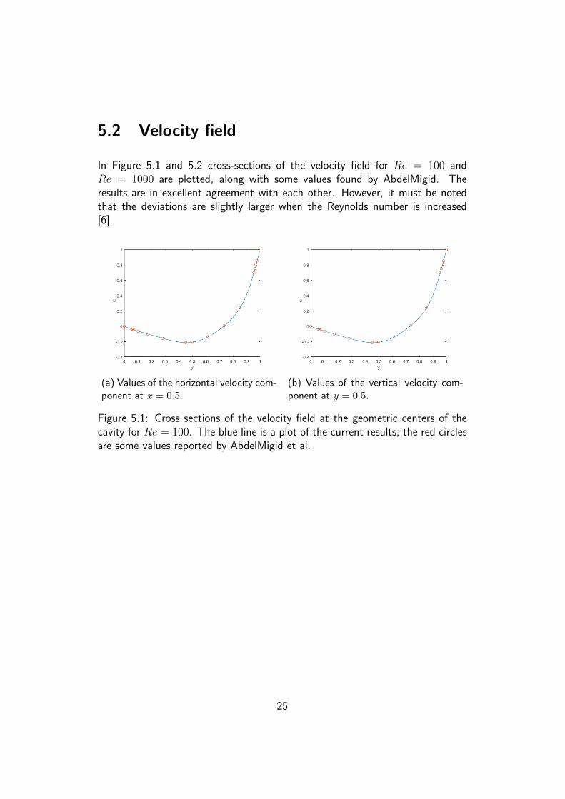
In Figure 5.1 and 5.2 cross-sections of the velocity field for Re = 100 andRe = 1000 are plotted, along with some values found by AbdelMigid. Theresults are in excellent agreement with each other. However, it must be notedthat the deviations are slightly larger when the Reynolds number is increased[6].
(a) Values of the horizontal velocity com-ponent at x = 0.5.
(b) Values of the vertical velocity com-ponent at y = 0.5.
Figure 5.1: Cross sections of the velocity field at the geometric centers of thecavity for Re = 100. The blue line is a plot of the current results; the red circlesare some values reported by AbdelMigid et al.
25

(a) Values of the horizontal velocity com-ponent at x = 0.5.
(b) Values of the vertical velocity com-ponent at y = 0.5.
Figure 5.2: Cross sections of the velocity field at the geometric centers of thecavity for Re = 1000. The blue line is a plot of the current results; the redcircles are some values reported by AbdelMigid et al.
5.3 Vorticity field
In Figure 5.3 the iso-stream function lines (stream lines) are shown for differentReynolds numbers. The primary vortex is clearly visible, as well as two secondaryvortices in the bottom corners of the cavity. For Re = 3200, the secondaryvortex in the left upper corner can also be observed.
In order to compare the flow with results in literature, the stream function ψ iscomputed using its definition
v = ∇× ψ,
from which follows that
u = −∂ψ∂y
v =∂ψ
∂x. (5.1)
The location of the primary vortex is determined by looking for the minimum ofthe stream function; the other vortices are local minima or maxima.
The coordinates of the primary vortex and some of its properties can be foundin Table 5.1 for Re = 100, Re = 400 and Re = 1000. They are compared toother results found by Ghia et al. [6] and AbdelMigid et al. [1]. Note that thesigns of the vorticity and stream function values are opposite. This is due to asign difference in the definition of the stream function [6]. Apart from that, thecurrent results are in good agreement with earlier studies. Note for example that
26

(a) Re = 100 (b) Re = 400
(c) Re = 1000 (d) Re = 3200
Figure 5.3: Stream lines of the velocity field (iso-Ψ-lines) for different Reynoldsnumbers.
27

Table 5.1: Vorticity value, stream function value and location of the primaryvortex for different Reynolds values for the present case and the results found byGhia et al. [3] in 1982 and AbdelMigid et al. [1] in 2016.
Re Reference Grid ω ψ (x,y)100 Present 129×129 -3.16549 0.103353 (0.6172, 0.7344)
Ghia et al. 129×129 3.16646 -0.103423 (0.6172, 0.7344)AbdelMigid et al. 601×601 3.15620 -0.103516 (0.6156, 0.7371)
400 Present 129×129 -2.28510 0.113216 (0.5547, 0.6094)Ghia et al. 129×129 2.29469 -0.113909 (0.5547, 0.6055)AbdelMigid et al. 601×601 2.29599 -0.113964 (0.5541, 0.6057)
1000 Present 129×129 -2.03741 0.116839 (0.5313, 0.5625)Ghia et al. 129×129 2.04968 -0.117929 (0.5313, 0.5625)AbdelMigid et al. 601×601 2.06658 -0.118866 (0.5308, 0.5657)
the position of the vortex is very good compared to the coordinates that Ghia etal. found, who used the same grid.
It is proven theoretically that there is a sequence of counter-rotating vortices inthe corners of the lid-driven cavity, called Moffatt vortices. Biswas and Kalita[2] were able to identify up to the quaternary vortex in the left and right bot-tom corner with a numerical study. With the current influence matrix method,secondary vortices could be distinguished in the bottom corners. Moreover, a ter-tiary vortex was found in the right bottom, although it was too small to depictadequately.
The properties of the secondary and tertiary vortices in the right corner canbe found in Table 5.2. For Re = 1000, the results are compared to thoseobtained by Biswas and Kalita. Although the coordinates of the vortices couldbe identified correctly, the values of the vorticity and stream function do notagree completely. These differences can be explained by the dissimilar grids thatwere used. The study of Moffatt vortices used a 321 × 321 non-homogeneousgrid, with relatively more points at the boundaries. Therefore, this was finer andbetter suited to give good results in the corners. In addition, Biswas and Kalitaused higher order discretization, which can also explain the differences.
28

Table 5.2: Properties of the Moffatt vortices in the bottom right corner for twodifferent Reynolds numbers. For Re = 1000, results found by Biswas and Kalita[2] are also given.
Re type study ω ψ (x,y)400 secondary present 0.4287 -0.000635 (0.8906, 0.1250)400 tertiary present -0.0044 1.442e-8 (0.9922, 0.0078)
1000 secondary present 0.11251 -0.001697 (0.8594, 0.1094)Biswas & Kalita 0.17539 0.001731 (0.8657, 0.1128)
1000 tertiary present -0.00867 3.670e-8 (0.9922, 0.0078)Biswas & Kalita 0.01045 -4.87726e-8 (0.9926, 0.0074)
29

Conclusion and discussion
The 2D Navier-Stokes equations were written in vorticity-velocity form and solvedwith an influence matrix technique developed by Daube [5]. The advantageof this method is that only boundary conditions for the velocity are needed.The boundary conditions for the vorticity are constructed using the influencematrix.
The technique was used to solve the classical problem of the lid-driven cavityflow. A homogeneous 129 × 129 grid was used for the discretization and theproblem was solved for Re = 100, Re = 400 and Re = 1000. As required fora 2D incompressible flow, the velocity field is divergence free and the definitionof the vorticity was satisfied. Both conditions yielded a result of O(10−13) orsmaller.
Compared to other results found in literature, the method performed very well.The velocity field was in excellent agreement with numbers found by AbdelMigidet al. [1]. The same applies for the location, stream function value and vorticityof the primary vortex.
Secondary and tertiary vortices in the bottom right corner were also investigatedfor Re = 400 and Re = 1000. For Re = 1000, the locations of the vorticeswere good compared to the coordinates found by Biswas and Kalita [2], but thevalues of the stream function and vorticity had larger deviations.
In order to improve the discretization, the grid could be more refined. Thisis especially important for the accuracy in case of higher Reynolds numbers.However, this comes with larger computation times. In addition, it might needsuch large matrices that it is likely that the code needs to be rewritten in orderto prevent MATLAB to use more than 100% of RAM.
Another solution is to use a non-homogeneous grid, which has relatively morepoints at the boundaries. This is also a reason why the study of Biswas and Kalitahad other results than the present method. This may be especially importantwhen the technique is used to study the behaviour of the flow near the boundaries
30

or in the corners of the domain.
This method can be used to solve other boundary value problems than the classi-cal lid-driven cavity flow. For instance, the aspect ratio of this standard problemcould be changed or a dipole could be placed in the center of the domain. Withslight modifications to compensate for cylindrical coordinates, the method canalso be used to study axisymmetric flows [5].
Finally, there are a couple of things that might optimize the Matlab code. Firstly,the sparse function is used after the construction of the coefficient matricesfor the computation of partial derivatives, Laplacians, et cetera. This functioncan be used in Matlab to make it recognize that a matrix is sparse, therebysaving memory and computation time. Using it during the construction of thesecoefficient matrices might save memory and time in the preprocessing stageof the algorithm. The second option to save computation time concerns thecalculation of inverses in the processing stage. Currently, matrix-vector equationsare solved with the Matlab operator \. If the inverses of the required matrices aredetermined in the preprocessing stage using LU-decomposition, each time steponly requires matrix multiplications and no inversions. This may save time.
31

Bibliography
[1] T. A. AbdelMigid, K. M. Saqr, M. A. Kotb, and A. A. Aboelfarag. Revisitingthe lid-driven cavity flow problem: Review and new steady state benchmark-ing results using GPU accelerated code. Alexandria Engineering Journal,56(1):123–135, 2017.
[2] S. Biswas and J. C. Kalita. Moffatt vortices in the lid-driven cavity flow.Journal of Physics: Conference Series, 759(1):012081, 2016.
[3] O. Botella and R. Peyret. Benchmark spectral results on the lid-driven cavityflow. Computers & Fluids, 27(4):421–433, 1998.
[4] H. J. H. Clercx. A spectral solver for the Navier-Stokes equations in thevelocity–vorticity formulation for flows with two nonperiodic directions. Jour-nal of Computational Physics, 137(1):186–211, 1997.
[5] O. Daube. Resolution of the 2D Navier-Stokes equations in velocity-vorticityform by means of an influence matrix technique. Journal of ComputationalPhysics, 103(2):402–414, 1992.
[6] U. K. N. G. Ghia, K. N. Ghia, and C. T. Shin. High-Re solutions for incom-pressible flow using the Navier-Stokes equations and a multigrid method.Journal of Computational Physics, 48(3):387–411, 1982.
[7] F. H. Harlow and J. E. Welch. Numerical calculation of time-dependentviscous incompressible flow of fluid with free surface. The Physics of Fluids,8(12):2182–2189, 1965.
[8] Y. He and W. Sun. Stability and convergence of the Crank–Nicolson/Adams–Bashforth scheme for the time-dependent Navier–Stokes equations. SIAMJournal on Numerical Analysis, 45(2):837–869, 2007.
[9] L. Skerget and Z. Rek. Boundary-domain integral method using avelocity-vorticity formulation. Engineering Analysis with Boundary Elements,15(4):359–370, 1995.
32

Appendix A
Derivation of the velocity-vorticityequation
The continuity equation states that mass is conserved. It reads
∂ρ
∂t+∇ · (ρv) = 0. (A.1)
Here, ρ is the density of the fluid and v is the velocity. If a flow is incompressible,this means that the density of the fluid is constant within an infinitesimal volumemoving with velocity v. That means that Dρ/Dt = 0, where Dρ/Dt = 0 isthe material derivative of ρ. In that case, the continuity equation is equivalentto
∇ · v = 0. (A.2)
Then, for a Newtonian fluid the Navier-Stokes equations read
∂v
∂t+ (v · ∇)v = −1
ρ∇p+ ν∇2v + g, (A.3)
where p is the pressure and g consists of the body forces on the fluid, includinggravity. Under the assumption that there are no such body forces, the equationsread
∂v
∂t+ (v · ∇)v = −1
ρ∇p+ ν∇2v, (A.4)
33

This equation can also be cast in dimensionless form, which is
∂v
∂t+ (v · ∇)v = −1
ρ∇p+
1
Re∇2v (A.5)
Here, Re is Reynolds number.
By definition, the vorticity v equals
∇× v = ω. (A.6)
The Navier-Stokes equations (A.5) can be rewritten by using the relation
(v · ∇)v = ∇(
1
2v · v
)− v × ω,
resulting in the equation
∂v
∂t+∇
(1
2v · v
)− v × ω = −1
ρ∇p+ ν∇2v. (A.7)
Taking the curl of the Navier-Stokes equations (A.7) and using the definition(A.6) of vorticity yields
∂ω
∂t+∇×∇
(1
2v · v
)−∇×(v×ω) = −∇×
(1
ρ∇p)
+∇×(ν∇2v
). (A.8)
In order to simplify this equation, the following identities will be used:
∇×∇φ = 0, (A.9)
∇2v = ∇(∇ · v)−∇× (∇× v), (A.10)
∇ · (∇× v) = ∇ · ω = 0, (A.11)
for an arbitrary scalar φ.
Then, equation (A.8) becomes
∂ω
∂t+∇×∇
(1
2v · v
)︸ ︷︷ ︸
=0 by (A.9)
−∇× (v × ω) = − ∇×(
1
ρ∇p)
︸ ︷︷ ︸=0 by (A.9),ρ constant
+∇×(ν∇2v
)∂ω
∂t−∇× (v × ω) = ∇×
(ν∇2v
)∂ω
∂t−∇× (v × ω) = ∇× (ν(∇ (∇ · v)︸ ︷︷ ︸
=0 by (A.2)
−∇× (∇× v)︸ ︷︷ ︸=ω
)).
34

The second term on the left-hand side can be rewritten by using
∇× (v × ω) = v(∇ · ω) + (ω · ∇)v − ω(∇ · v)− (v · ∇)ω.
Together with equations (A.11) and (A.2) this results in
∂ω
∂t− v (∇ · ω)︸ ︷︷ ︸
=0 by (A.11)
−(ω · ∇)v + ω (∇ · v)︸ ︷︷ ︸=0 by (A.2)
+(v · ∇)ω = −ν(∇× (∇× ω))
∂ω
∂t− (ω · ∇)v + (v · ∇)ω = −ν(∇× (∇× ω)).
Using relation (A.10) for ω instead of v gives
∇2ω = ∇(∇ · ω)−∇× (∇× ω) = −∇× (∇× ω).
because of equation (A.11). Rearranging terms and using the condition thatthere are no body forces then gives
∂ω
∂t+ (v · ∇)ω = (ω · ∇)v + ν(∇2ω). (A.12)
In this equation ∂ω∂t
describes the unsteadyness in the flow, which contributes tothe rate of change of the vorticity in a fixed infinitesimally small volume. Theother term on the left-hand side is the convection term, which describes the rateof change of the vorticity as this volume moves through the fluid. The first termon the right-hand side describes stretching or tilting of the velocity due to thegradients in the flow velocity. The final term on the right-hand side describesthe diffusion of the vorticity through the fluid.
Equation (A.12) can be applied whenever the flow is incompressible, the fluidNewtonian and when there are no body forces. If the extra assumption is madethat the flow is two-dimensional, then ω = ωk, where k is the unit vector inthe z-direction. With v = ui + vj and the continuity equation (A.1), we canwrite
∇ · (ωv) = ∂x(ωu) + ∂y(ωv)
= u∂xω + ω∂xu+ v∂yω + ω∂yv
= u∂xω + v∂yω + ω(∂xu+ ∂yv)
= u∂xω + v∂yω
= (v · ∇)ω.
35

Equation (1.4) can then be simplified to
∂ω
∂t+∇ · (ωv) = ν∇2ω. (A.13)
36
Appendix B
Matlab scripts
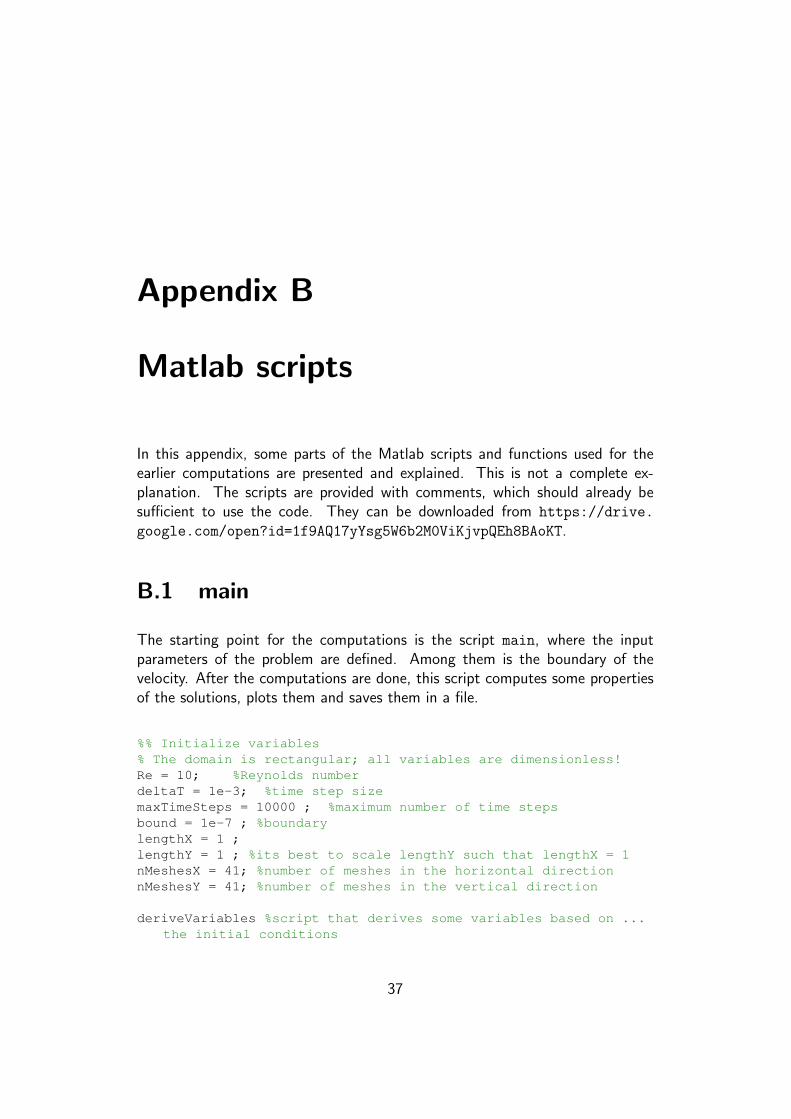
In this appendix, some parts of the Matlab scripts and functions used for theearlier computations are presented and explained. This is not a complete ex-planation. The scripts are provided with comments, which should already besufficient to use the code. They can be downloaded from https://drive.
google.com/open?id=1f9AQ17yYsg5W6b2M0ViKjvpQEh8BAoKT.
B.1 main
The starting point for the computations is the script main, where the inputparameters of the problem are defined. Among them is the boundary of thevelocity. After the computations are done, this script computes some propertiesof the solutions, plots them and saves them in a file.
%% Initialize variables% The domain is rectangular; all variables are dimensionless!Re = 10; %Reynolds numberdeltaT = 1e-3; %time step sizemaxTimeSteps = 10000 ; %maximum number of time stepsbound = 1e-7 ; %boundarylengthX = 1 ;lengthY = 1 ; %its best to scale lengthY such that lengthX = 1nMeshesX = 41; %number of meshes in the horizontal directionnMeshesY = 41; %number of meshes in the vertical direction
deriveVariables %script that derives some variables based on ...the initial conditions
37

%% Define problem: boundary conditions for velocity (corners ...are zero because it otherwise yields problems with the ...solutions)
velocityBoundary.horizontal.upper = ...ones(1,nHorizontalVelocityCols) ;
velocityBoundary.horizontal.upper(1,1) = 0 ;velocityBoundary.horizontal.upper(1,nHorizontalVelocityCols) ...
= 0 ;velocityBoundary.horizontal.right = ...
zeros(nInnerHorizontalVelocityRows, 1) ;velocityBoundary.horizontal.lower = zeros(1, ...
nHorizontalVelocityCols) ;velocityBoundary.horizontal.left = ...
zeros(nInnerHorizontalVelocityRows, 1) ;
velocityBoundary.vertical.upper = zeros(1, ...nInnerVerticalVelocityCols) ;
velocityBoundary.vertical.right = ...zeros(nVerticalVelocityRows, 1) ;
velocityBoundary.vertical.lower = zeros(1, ...nInnerVerticalVelocityCols) ;
velocityBoundary.vertical.left = ...zeros(nVerticalVelocityRows, 1) ;
%% Compute solution%solveProblemSteadyState() solves the problem until a ...
certain steady state%and gives only this steady state result as solution (the ...
rest of the%information is lost). solveProblem() also gives the ...
intermediate results%and puts the results of all time steps into an array. The ...
drawback of this%is the amount of memory that is needed.
[solution, timesteps] = ...solveProblemSteadyState(velocityBoundary, Re, bound, ...maxTimeSteps, deltaT, nMeshesX, nMeshesY, lengthX, ...lengthY) ;
%[solutionArray, timestepsArray, elementaryProblemArray, ...givenProblemArray] = solveProblem(velocityBoundary, Re, ...bound, maxTimeSteps, deltaT, nMeshesX, nMeshesY, lengthX, ...lengthY) ;
% Display some parameters and results of the computation ;fprintf('Re: %d \n', Re) ;fprintf('deltaX: %d \n', deltaX);fprintf('deltaY: %d \n', deltaY);fprintf('deltaT: %d \n', deltaT);
38

fprintf('time: %d \n', (timesteps-1) * deltaT);
maximumVorticity = max(max(solution.vorticity)) ;minimumVorticity = min(min(solution.vorticity)) ;rmsFinal = solution.rms ;
fprintf('maximum vorticity: %d \n', maximumVorticity) ;fprintf('minimum vorticity: %d \n', minimumVorticity) ;
%% Plot some solutions of the problemname = strcat(' Re = ', num2str(Re), ' ', num2str(nMeshesX), ...
'x', num2str(nMeshesY)) ; %add a name for the plots ...(giving information about Reynolds number and grid size)
[u, v] = plotReportSolutions(solution, nMeshesX, nMeshesY, ...lengthX, lengthY, velocityBoundary, name) ;
plotCrossSections(solution, nMeshesX, nMeshesY, lengthX, ...lengthY, Re, name) ;
%% Determine position of the primary vortex of the solutionmaximumStreamfunction = max(max(solution.streamfunction)) ; ...
%compute the maximum of the stream function
[jMaxPsi, iMaxPsi] = find(solution.streamfunction == ...maximumStreamfunction) ; %find the location of the ...maximum of the streamfunction
xMaxPsi = deltaX*(iMaxPsi-1) ;yMaxPsi = deltaY*(jMaxPsi-1) ;
minimumStreamfunction = min(min(solution.streamfunction)) ; ...%compute the minimum of the stream function
[jMinPsi, iMinPsi] = find(solution.streamfunction == ...minimumStreamfunction) ; %find the location of the ...minimum of the streamfunction
xMinPsi = deltaX*(iMinPsi-1) ; %compute the corresponding x ...and y values
yMinPsi = deltaY*(jMinPsi-1) ;
%display the maximum/minimum stream functionfprintf('maximum stream function: %d at (%d, %d) \n', ...
maximumStreamfunction, xMaxPsi, yMaxPsi) ;fprintf('vorticity at this point: %d \n', ...
solution.vorticity(jMaxPsi, iMaxPsi)) ;
fprintf('minimum stream function: %d at (%d, %d) \n', ...minimumStreamfunction, xMinPsi, yMinPsi) ;
fprintf('vorticity at this point: %d \n', ...solution.vorticity(jMinPsi, iMinPsi)) ;
39

%% Write to filepath = 'C:\' ; %Choose your own path herefolder = strcat('Re', num2str(Re), '\') ; %Place it in the ...
folder ReN, where N is the Reynolds number (folder needs ...to be created before it can be saved there)
filename = strcat(num2str(nMeshesX), 'x', num2str(nMeshesY)) ...; %Filename will be the grid size, e.g. '129x129'
totalPath = strcat(path, folder, filename) ;
save(totalPath, 'solution', 'Re', 'nMeshesX', 'nMeshesY', ...'deltaX', 'deltaY', 'deltaT', 'timesteps', 'bound', ...'-v7.3') ;
B.2 solveProblemSteadyState()
The function solveProblemSteadyState is called in the main script. This isactually the most important function. This is where the ’real’ calculations aredone. It returns the steady state solution of the problem and the amount of timesteps that was needed to get to that steady state.
The function solveProblem does the same calculations, but returns an arraywith all intermediate solutions. These include the solutions of the elementaryproblems Ek and given problem B in equations (1.32) and (1.30), respectively.This requires a lot of memory. Hence, it is strongly advised to use this functiononly to understand the computations or when intermediate solutions are neededfor any other reason.
At the beginning of solveProblemSteadyState, the functioncreateCoefficientMatrices is called. This function creates all necessarymatrices for the computation of partial derivatives, divergences, rotations etcetera. These are used as argument in many other functions.
function [solution, finalTimeStep] = ...solveProblemSteadyState(velocityBoundary, Re, bound, ...maxTimesteps, deltaT, nMeshesX, nMeshesY, lengthX, lengthY)
%SOLVEPROBLEMSTEADYSTATE This function returns the steady ...state solution
%of the problem that is defined in the arguments% The VELOCITYBOUNDARY is the vorticity boundary that is ...
used in the% first time step. RE is the Reynolds number. BOUND is the ...
difference
40

% between maxima of two consecutively computed quantities ...for which it
% is believed that there is a steady state. MAXTIMESTEPS ...is the maximum
% number of time steps that the script should take. DELTAT ...is the time
% step size. NMESHESX and NMESHESY are the amount of ...meshes in the x-
% and y-direction, respectively.% The function returns the SOLUTION struct with vorticity ...
and velocity% field components of the steady state solution, along ...
with some% properties of this solution: the difference between the ...
rotation of% the velocity field and the vorticity (should be zero), ...
the divercenge% of the velocity field (should also be zero) and the ...
RMS-value of the% velocity field.% The algorithm is based on an article written by O. Daube ...
in 1992,% titled 'Resolution of the 2D Navier-Stokes Equations in% Velocity-Vorticity Form by Means of an Influence Matrix ...
Technique'.
%% Derive some variables for the computationdeltaX = lengthX/(nMeshesX-1); %step size in the horizontal ...
directiondeltaY = lengthY/(nMeshesY-1); %step size in the vertical ...
directionsigma = 2*Re / deltaT ;
nVorticityRows = nMeshesY ;nVorticityCols = nMeshesX ;nInnerVorticityRows = nMeshesY - 2;nInnerVorticityCols = nMeshesX - 2;
nHorizontalVelocityRows = nMeshesY - 1;nHorizontalVelocityCols = nMeshesX ;
nVerticalVelocityRows = nMeshesY;nVerticalVelocityCols = nMeshesX - 1;
nBoundaryPoints = 2*nMeshesX + 2*nMeshesY - 4 - 4; %number ...of boundary points except the corners
%% Create coefficient matrices for the calculationscoefficientMatrices = createCoefficientMatrices(sigma, ...
41

nMeshesX, nMeshesY, lengthX, lengthY) ;
%% Set timer for the execution timetic
%% Solve elementary problemselementaryProblem = solveElementaryProblems(nMeshesX, ...
nMeshesY, coefficientMatrices) ;disp('elementary problems solved');
%% Create influence matrixinfluenceMatrix = zeros(nBoundaryPoints, nBoundaryPoints) ;for k = 1:nBoundaryPoints
influenceMatrix(:, k) = ...elementaryProblem(k).vorticityDifference ;
enddisp('influence matrix constructed');
%% Define the boundary that will be used as the initial ...'guess' for the given problem (omega-tilde)
%Define a distribution for the vorticity on the boundary ...(all defined from
%left to right or up to downconstantNegative = -1 ;vorticityBoundary.upper = constantNegative*ones(1,nMeshesX) ;vorticityBoundary.right = ...
constantNegative*ones(nMeshesY-2,1) ;vorticityBoundary.lower = constantNegative*ones(1,nMeshesX) ;vorticityBoundary.left = constantNegative*ones(nMeshesY-2,1) ;
%% Preallocate and set initial variables
for i = 3:-1:1givenProblem(i).innerVorticity = ...
zeros(nInnerVorticityRows, nInnerVorticityCols) ;givenProblem(i).vorticity = zeros(nVorticityRows, ...
nVorticityCols) ;
givenProblem(i).horizontalVelocity = ...zeros(nHorizontalVelocityRows, ...nHorizontalVelocityCols) ;
givenProblem(i).verticalVelocity = ...zeros(nVerticalVelocityRows, nVerticalVelocityCols) ;
givenProblem(i).vorticityBoundaryMatrix = ...zeros(nInnerVorticityRows, nInnerVorticityCols) ;
end
42

isSteady = 0 ;i = 1 ;
%% Start the calculations!while isSteady == 0 && i <= maxTimesteps
if i == 1 %for the first time step, use the ...vorticity boundary defined abovegivenProblem(1).vorticityBoundary.lower = ...
vorticityBoundary.lower;givenProblem(1).vorticityBoundary.right = ...
vorticityBoundary.right;givenProblem(1).vorticityBoundary.upper = ...
vorticityBoundary.upper;givenProblem(1).vorticityBoundary.left = ...
vorticityBoundary.left;else %for the others, use the vorticity boundary of ...
the solution of the previous time stepgivenProblem(1).vorticityBoundary.lower = ...
solution.vorticity(1,:) ;givenProblem(1).vorticityBoundary.right = ...
solution.vorticity(2:nMeshesY-1,nMeshesX) ;givenProblem(1).vorticityBoundary.upper = ...
solution.vorticity(nMeshesY,:) ;givenProblem(1).vorticityBoundary.left = ...
solution.vorticity(2:nMeshesY-1,1) ;end
%set the boundaries of the vorticity according to ...what is defined
%above and make the matrix (will be converted to a ...vector) that
%will be added to the RHS of the equationgivenProblem(1).vorticity(1,2:nVorticityCols-1) = ...
givenProblem(1).vorticityBoundary.lower(1,2:nVorticityCols-1);givenProblem(1).vorticity(2:nMeshesY-1,nMeshesX) = ...
givenProblem(1).vorticityBoundary.right;givenProblem(1).vorticity(nMeshesY,2:nVorticityCols-1) ...
= ...givenProblem(1).vorticityBoundary.upper(1,2:nVorticityCols-1);
givenProblem(1).vorticity(2:nMeshesY-1,1) = ...givenProblem(1).vorticityBoundary.left;
givenProblem(1).vorticityBoundaryMatrix(1,:) = ...givenProblem(1).vorticityBoundaryMatrix(1,:) + ...givenProblem(1).vorticityBoundary.lower(1,2:nMeshesX-1) .../ deltaYˆ2 ;
givenProblem(1).vorticityBoundaryMatrix(:,nInnerVorticityCols) ...= ...
43

givenProblem(1).vorticityBoundaryMatrix(:,nInnerVorticityCols) ...+ givenProblem(1).vorticityBoundary.right / ...deltaXˆ2 ;
givenProblem(1).vorticityBoundaryMatrix(nInnerVorticityRows, ...:) = ...givenProblem(1).vorticityBoundaryMatrix(nInnerVorticityRows, ...:) + ...givenProblem(1).vorticityBoundary.upper(1,2:nMeshesX-1) .../ deltaYˆ2 ;
givenProblem(1).vorticityBoundaryMatrix(:, 1) = ...givenProblem(1).vorticityBoundaryMatrix(:, 1) + ...givenProblem(1).vorticityBoundary.left / deltaXˆ2;
%With this information, create the right hand side ...of the Helmholz equation for the given problems ...for this time step
if i == 1term1 = givenProblem(2).vorticityBoundaryMatrix ;givenProblem(1).RHS = term1 + ...
givenProblem(1).vorticityBoundaryMatrix ;elseif i == 2
givenProblem(2).divergenceTerm = ...createDivergenceTerm(givenProblem(2), ...coefficientMatrices) ;
givenProblem(2).nonHomogeneousTerm = ...createNonHomogeneousTerm(givenProblem(2), ...givenProblem(2), coefficientMatrices, Re, 1) ;
givenProblem(1).RHS = ...givenProblem(2).nonHomogeneousTerm + ...givenProblem(1).vorticityBoundaryMatrix ;
elsegivenProblem(2).divergenceTerm = ...
createDivergenceTerm(givenProblem(2), ...coefficientMatrices) ;
givenProblem(2).nonHomogeneousTerm = ...createNonHomogeneousTerm(givenProblem(2), ...givenProblem(3), coefficientMatrices, Re, 0) ;
givenProblem(1).RHS = ...givenProblem(2).nonHomogeneousTerm + ...givenProblem(1).vorticityBoundaryMatrix ;
end
%Calculate the vorticity solutions for this time stepgivenProblem(1).innerVorticity = ...
multiplyMatrixWithInverseMatrix(coefficientMatrices.innerVorticity, ...givenProblem(1).RHS, nInnerVorticityCols) ;
givenProblem(1).vorticity(2:nMeshesY-1, ...2:nMeshesX-1) = givenProblem(1).innerVorticity ;
44

%Calculate the solutions for the velocities for this ...time step
[givenProblem(1).horizontalVelocity, ...givenProblem(1).verticalVelocity] = ...solvePoissonEquation(givenProblem(1), ...velocityBoundary, coefficientMatrices, deltaX, ...deltaY);
%Calculate coefficients for the influence matrixrotationVelocityVector = ...
calculateRotationBoundary(givenProblem(1).horizontalVelocity, ...givenProblem(1).verticalVelocity, ...coefficientMatrices, velocityBoundary);
vorticityBoundary = ...[transpose(givenProblem(1).vorticityBoundary.lower(1,2:nVorticityCols-1)); ...givenProblem(1).vorticityBoundary.right; ...flip(transpose(givenProblem(1).vorticityBoundary.upper(1,2:nVorticityCols-1))); ...flip(givenProblem(1).vorticityBoundary.left)];
vorticityDifference = rotationVelocityVector - ...vorticityBoundary ;
%compute the real solution by first calculating the ...necessary
%correctionsvorticitySum = zeros(nVorticityRows, nVorticityCols);horizontalVelocitySum = ...
zeros(nHorizontalVelocityRows, ...nHorizontalVelocityCols);
verticalVelocitySum = zeros(nVerticalVelocityRows, ...nVerticalVelocityCols);
coefficients = influenceMatrix \ ...-vorticityDifference ;
for k = 1:nBoundaryPointsvorticitySum = vorticitySum + coefficients(k) * ...
elementaryProblem(k).vorticity ;horizontalVelocitySum = horizontalVelocitySum + ...
coefficients(k) * ...elementaryProblem(k).horizontalVelocity ;
verticalVelocitySum = verticalVelocitySum + ...coefficients(k) * ...elementaryProblem(k).verticalVelocity ;
end
if i > 1solutionOld = solution ; %store the old solution ...
in order to compute if there is a steady stateend
45

solution.vorticity = givenProblem(1).vorticity + ...vorticitySum ; %add correction to given problem ...to get the real solution
solution.horizontalVelocity = ...givenProblem(1).horizontalVelocity + ...horizontalVelocitySum ;
solution.verticalVelocity = ...givenProblem(1).verticalVelocity + ...verticalVelocitySum ;
%check if there is a steady stateif i > 1 %this cannot be calculated after the first ...
time step[isSteady, solution.valueHor, solution.valueVer, ...
solution.valueVor] = testSteadyState(bound, ...solution, solutionOld, deltaT);
elsesolution.valueVor = 0 ;
end
fprintf('time step %d ready, vorticity difference %d ...\n', i, solution.valueVor);
%change givenProblems and set timestep counter to ...get ready for the
%next time step!givenProblem(3) = givenProblem(2) ;givenProblem(2) = givenProblem(1) ;givenProblem(1).vorticityBoundaryMatrix = ...
zeros(nInnerVorticityRows, nInnerVorticityCols) ;i = i + 1 ;
end
finalTimeStep = i - 1;
executionTime = toc ;
fprintf('solution computed in %d seconds \n', executionTime);
%% compute some properties of the solutionrotation = calculateRotation(solution.horizontalVelocity, ...
solution.verticalVelocity, velocityBoundary, ...coefficientMatrices); %calculate the rotation of the ...velocity field
solution.rotationDifference = max(max(abs(rotation - ...solution.vorticity))) ; %this should be (practically) 0
solution.divergence = ...max(max(abs(checkDivergence(solution.horizontalVelocity, ...
46

solution.verticalVelocity, coefficientMatrices)))) ; ...%velocity field should be divergence free
solution.rms = ...computeRMSvelocity(solution.horizontalVelocity, ...solution.verticalVelocity, velocityBoundary) ; %compute ...root mean square of the velocity field
solution.streamfunction = calculateStreamFunction(deltaX, ...deltaY, solution.horizontalVelocity, ...solution.verticalVelocity, velocityBoundary) ;
end
B.3 solveElementaryProblems()
The function solveElementaryProblems solves the elementary problems de-fined in equation (1.32).
function [elementaryProblem] = ...solveElementaryProblems(nMeshesX, nMeshesY, ...coefficientMatrices)
%SOLVEELEMENTARYPROBLEMS This function solves the elementary ...problems
%%% Create the boundary vectors. These are defined from 1 to ...
nBoundaryPoints%%in the clockwise direction, starting from the upper left ...
point (1,1).
deltaX = 1/(nMeshesX-1); %step size in the horizontal directiondeltaY = 1/(nMeshesY-1); %step size in the vertical direction
nVorticityRows = nMeshesY ;nVorticityCols = nMeshesX ;nInnerVorticityRows = nMeshesY - 2;nInnerVorticityCols = nMeshesX - 2;
nHorizontalVelocityCols = nMeshesX ;nInnerHorizontalVelocityRows = nMeshesY - 1 ;
nVerticalVelocityRows = nMeshesY;nInnerVerticalVelocityCols = nMeshesX - 1 ;
nBoundaryPoints = 2*nInnerVorticityRows + ...2*nInnerVorticityCols ; %number of boundary points except ...
47

the corners
%% Define problem: boundary conditions for velocity
elementaryVelocityBoundary.horizontal.upper = ...zeros(1,nHorizontalVelocityCols) ;
elementaryVelocityBoundary.horizontal.right = ...zeros(nInnerHorizontalVelocityRows, 1) ;
elementaryVelocityBoundary.horizontal.lower = zeros(1, ...nHorizontalVelocityCols) ;
elementaryVelocityBoundary.horizontal.left = ...zeros(nInnerHorizontalVelocityRows, 1) ;
elementaryVelocityBoundary.vertical.upper = zeros(1, ...nInnerVerticalVelocityCols) ;
elementaryVelocityBoundary.vertical.right = ...zeros(nVerticalVelocityRows, 1) ;
elementaryVelocityBoundary.vertical.lower = zeros(1, ...nInnerVerticalVelocityCols) ;
elementaryVelocityBoundary.vertical.left = ...zeros(nVerticalVelocityRows, 1) ;
%%This part of the script finds a solution for the ...elementary problems Ek.
%%Firstly, a solution to the first equations for the omega ...hats is
%%constructed. It involves computing a solution of the ...matrix equation
%%A*omega=b, where A is a (Nx+Ny-4, Nx+Ny-4) matrix with the ...coefficients corresponding to
%%second order centered differences. The vector omega ...consists of the
%%variables omega hat to be computed and in b the boundary ...conditions will
%%be put.
%At the boundaries, the coefficients for the velocity ...solutions are not
%exactly the coefficients corresponding to the Laplacian, ...due to virtual
%points that are used. Therefore, the matrices must be ...corrected such that
%the coefficients at the boundaries are correct.
%% Create/preallocate the elementary problems and fix the ...boundaries
%Define the indices of the cornersleftLower = 1 ;
48

rightLower = nInnerVorticityCols ;rightUpper = nInnerVorticityCols + nInnerVorticityRows ;leftUpper = 2*nInnerVorticityCols + nInnerVorticityRows ;
%Define the vorticity boundaries for the elementary ...problems. Counting will
%start at the left corner of the bottom boundary, going ...anti-clockwise.
for k = nBoundaryPoints:-1:1 %backwards for preallocationelementaryProblem(k).vorticityBoundaryMatrix = ...
zeros(nInnerVorticityRows, nInnerVorticityCols) ;elementaryProblem(k).vorticity = zeros(nVorticityRows, ...
nVorticityCols) ;if (k >= leftLower && k <= rightLower) % k is a point on ...
the lower boundaryelementaryProblem(k).vorticityBoundaryMatrix(1, k) = ...
-1/deltaYˆ2;elementaryProblem(k).vorticity(1, k+1) = 1 ;
elseif (k > rightLower && k <= rightUpper) % k is a point ...on the right boundaryj = k - rightLower ;elementaryProblem(k).vorticityBoundaryMatrix(j,nInnerVorticityCols) ...
= -1/deltaXˆ2 ;elementaryProblem(k).vorticity(j+1,nVorticityCols) = ...
1 ;elseif (k > rightUpper && k <= leftUpper) %k is a point ...
on the upper boundaryj = leftUpper - k + 1 ;elementaryProblem(k).vorticityBoundaryMatrix(nInnerVorticityRows,j) ...
= -1/deltaYˆ2;elementaryProblem(k).vorticity(nVorticityRows,j+1) = ...
1 ;elseif (k > leftUpper && k <= nBoundaryPoints) %k is a ...
point on the left boundaryj = nBoundaryPoints - k + 1 ;elementaryProblem(k).vorticityBoundaryMatrix(j, 1) = ...
-1/deltaXˆ2;elementaryProblem(k).vorticity(j+1, 1) = 1 ;
endend
%% Solve the elementary problemsfor k=1:nBoundaryPoints
% Solve the elementary problems for the vorticityelementaryProblem(k).vorticityRHS = - ...
elementaryProblem(k).vorticityBoundaryMatrix ;elementaryProblem(k).innerVorticity = ...
multiplyMatrixWithInverseMatrix(coefficientMatrices.innerVorticity, ...elementaryProblem(k).vorticityRHS, ...
49

nInnerVorticityCols); %calculate solution (vector)elementaryProblem(k).vorticity(2:nVorticityRows-1, ...
2:nVorticityCols-1) = ...elementaryProblem(k).innerVorticity;
% Solve the elementary problems for the velocities[elementaryProblem(k).horizontalVelocity, ...
elementaryProblem(k).verticalVelocity] = ...solvePoissonEquation(elementaryProblem(k), ...elementaryVelocityBoundary, coefficientMatrices, ...deltaX, deltaY);
% Compute the difference between the rotation of the ...velocity field and
% the prescribed 'vorticity' boundary valueelementaryProblem(k).rotationVelocityVector = ...
calculateRotationBoundary(elementaryProblem(k).horizontalVelocity, ...elementaryProblem(k).verticalVelocity, ...coefficientMatrices, elementaryVelocityBoundary);
boundary = zeros(nBoundaryPoints, 1) ;boundary(k,1) = 1 ;elementaryProblem(k).vorticityDifference = ...
elementaryProblem(k).rotationVelocityVector - ...boundary ;
end
end
B.4 createNonHomogeneousTerm()
The function createNonHomogeneousTerm computes the term S(n) of equation(1.17). This is used to find the vorticity values with equation (1.30a).
function nonHomogeneousTerm = ...createNonHomogeneousTerm(givenProblem2, givenProblem1, ...coefficientMatrices, Re, firstStep)
%COMPUTELAPLACIAN Summary of this function goes here% Detailed explanation goes here
nMeshesX = size(givenProblem2.vorticity, 2);
nVorticityCols = nMeshesX ;nInnerVorticityCols = nVorticityCols - 2 ;
50

%Compute the first term of Sterm1 = ...
multiplyMatrixWithMatrix(coefficientMatrices.vorticityHelmholzInner, ...givenProblem2.innerVorticity, nInnerVorticityCols) + ...givenProblem2.vorticityBoundaryMatrix ;
%Compute the second and third term of S(n)if (firstStep == 1)
%If it is the first time step, use Forward Eulerterm2 = - 2 * Re * givenProblem2.divergenceTerm ;term3 = zeros(size(givenProblem2.divergenceTerm)) ;
elseterm2 = - 3 * Re * givenProblem2.divergenceTerm ;term3 = Re * givenProblem1.divergenceTerm ;
end
%The sum of these terms is S(n)nonHomogeneousTerm = term1 + term2 + term3 ;
end
B.5 solvePoissonEquation()
The function solvePoissonEquation is used for the computation of the velocityfield when the vorticity is calculated. It is used in both the resolution of the givenproblem (1.30) and of the elementary problems (1.32). Therefore, it is called insolveProblemSteadyState and solveElementaryProblems.
function [horizontalVelocity, verticalVelocity] = ...solvePoissonEquation(problem, velocityBoundary, ...coefficientMatrices, deltaX, deltaY)
%SOLVEPOISSONEQUATION Summary of this function goes here% Detailed explanation goes here
nMeshesX = size(problem.vorticity, 2);nMeshesY = size(problem.vorticity, 1);
nHorizontalVelocityRows = nMeshesY - 1;nHorizontalVelocityCols = nMeshesX ;nInnerHorizontalVelocityRows = nMeshesY - 1;nInnerHorizontalVelocityCols = nMeshesX - 2;
nVerticalVelocityRows = nMeshesY;nVerticalVelocityCols = nMeshesX - 1;nInnerVerticalVelocityRows = nMeshesY - 2;
51

nInnerVerticalVelocityCols = nMeshesX - 1;
%Preallocate space and fix the boundaries (which are NOT ...zero)
horizontalVelocity = zeros(nHorizontalVelocityRows, ...nHorizontalVelocityCols) ;
horizontalVelocity(:,1) = ...velocityBoundary.horizontal.left ;
horizontalVelocity(:,nHorizontalVelocityCols) = ...velocityBoundary.horizontal.right ;
verticalVelocity = zeros(nVerticalVelocityRows, ...nVerticalVelocityCols) ;
verticalVelocity(1,:) = velocityBoundary.vertical.lower ;verticalVelocity(nVerticalVelocityRows, :) = ...
velocityBoundary.vertical.upper ;
%% Create boundaries for the velocity, construct ...boundary matrix
horizontalVelocityBoundaryMatrix = ...zeros(nInnerHorizontalVelocityRows, ...nInnerHorizontalVelocityCols) ;
horizontalVelocityBoundaryMatrix(1,:) = 8/3/deltaYˆ2 .* ...velocityBoundary.horizontal.lower(1, ...2:nHorizontalVelocityCols-1) ;
horizontalVelocityBoundaryMatrix(nInnerHorizontalVelocityRows, ...:) = 8/3/deltaYˆ2 .* ...velocityBoundary.horizontal.upper(1, ...2:nHorizontalVelocityCols-1) ;
horizontalVelocityBoundaryMatrix(:, 1) = ...horizontalVelocityBoundaryMatrix(:, 1) + 1/deltaXˆ2 ....* velocityBoundary.horizontal.left ;
horizontalVelocityBoundaryMatrix(:, ...nInnerHorizontalVelocityCols) = ...horizontalVelocityBoundaryMatrix(:, ...nInnerHorizontalVelocityCols) + 1/deltaXˆ2 .* ...velocityBoundary.horizontal.right ;
verticalVelocityBoundaryMatrix = ...zeros(nInnerVerticalVelocityRows, ...nInnerVerticalVelocityCols) ;
verticalVelocityBoundaryMatrix(:, 1) = 8/3/deltaXˆ2 .* ...velocityBoundary.vertical.left(2:nVerticalVelocityRows-1, ...1) ;
verticalVelocityBoundaryMatrix(:, ...nInnerVerticalVelocityCols) = 8/3/deltaXˆ2 .* ...velocityBoundary.vertical.right(2:nVerticalVelocityRows-1, ...1) ;
52

verticalVelocityBoundaryMatrix(1, :) = ...verticalVelocityBoundaryMatrix(1, :) + 1/deltaYˆ2 .* ...velocityBoundary.vertical.lower ;
verticalVelocityBoundaryMatrix(nInnerVerticalVelocityRows, ...:) = ...verticalVelocityBoundaryMatrix(nInnerVerticalVelocityRows, ...:) + 1/deltaYˆ2 .* velocityBoundary.vertical.upper ;
%% Solve the problempartialVorticityY = ...
multiplyMatrixWithMatrix(coefficientMatrices.partialVorticityY, ...problem.vorticity, nHorizontalVelocityCols);
partialVorticityX = ...multiplyMatrixWithMatrix(coefficientMatrices.partialVorticityX, ...problem.vorticity, nVerticalVelocityCols) ;
partialVorticityYInner = partialVorticityY(:, ...2:nHorizontalVelocityCols-1);
partialVorticityXInner = ...partialVorticityX(2:nVerticalVelocityRows-1, :);
horizontalVelocityRHS = - partialVorticityYInner - ...horizontalVelocityBoundaryMatrix ;
innerHorizontalVelocity = ...multiplyMatrixWithInverseMatrix(coefficientMatrices.horizontalVelocity, ...horizontalVelocityRHS, nInnerHorizontalVelocityCols);
horizontalVelocity(:, 2:nHorizontalVelocityCols-1) = ...innerHorizontalVelocity;
verticalVelocityRHS = partialVorticityXInner - ...verticalVelocityBoundaryMatrix ;
innerVerticalVelocity = ...multiplyMatrixWithInverseMatrix(coefficientMatrices.verticalVelocity, ...verticalVelocityRHS, nInnerVerticalVelocityCols);
verticalVelocity(2:nVerticalVelocityRows-1, :) = ...innerVerticalVelocity ;
end
B.6 multiplyMatrixWithMatrix()
The function multiplyMatrixWithMatrix and the related functionmultiplyMatrixWithInverseMatrix are some of the most important auxiliaryfunctions. These are used whenever quantities on the rectangular grid mustbe stored in a vector in order to compute partial derivatives, divergences, etcetera. The argument multiplicationMatrix is the coefficient matrix, for
53

example matrix M in equation (3.8). MultipliedMatrix is a matrix of vorticityor velocity values. The function stores the values of multipliedMatrix in avector and performs a matrix-vector multiplication. Next, the output vector istransformed back to a matrix.
function [resultMatrix, resultVector] = ...multiplyMatrixWithMatrix(multiplicationMatrix, ...multipliedMatrix, nColsOut)
%MULTIPLYMATRIXWITHMATRIX Multiplies matrix with matrix% This function converts multipliedMatrix in a vector in ...
order to perfom% the matrix multiplication. The amount of columns of% multiplicationMatrix must correstpond to the amount of ...
elements of the% multipliedMatrix.
%% sectionnRowsMultiplied = size(multipliedMatrix, 1);nColsMultiplied = size(multipliedMatrix, 2);
nMultipliedElements = nRowsMultiplied * nColsMultiplied ;
%transform matrix in vector by putting all elements row-wise ...in a column
%vectormultipliedVector = reshape(multipliedMatrix.', ...
[nMultipliedElements,1]) ;resultVector = multiplicationMatrix * multipliedVector ;
%put the elements of the vector in a matrix with nColsOut ...columns
%(row-wise)resultMatrix = vec2mat(resultVector, nColsOut);
end
54