Embed Size (px)
Citation preview

Eindhoven University of Technology
MASTER
A multi echelon safety stock setting procedure using simulation
coping with supply and demand uncertainties in the animal health industry
Teunissen, B.
Award date:2009
DisclaimerThis document contains a student thesis (bachelor's or master's), as authored by a student at Eindhoven University of Technology. Studenttheses are made available in the TU/e repository upon obtaining the required degree. The grade received is not published on the documentas presented in the repository. The required complexity or quality of research of student theses may vary by program, and the requiredminimum study period may vary in duration.
General rightsCopyright and moral rights for the publications made accessible in the public portal are retained by the authors and/or other copyright ownersand it is a condition of accessing publications that users recognise and abide by the legal requirements associated with these rights.
• Users may download and print one copy of any publication from the public portal for the purpose of private study or research. • You may not further distribute the material or use it for any profit-making activity or commercial gain
Take down policyIf you believe that this document breaches copyright please contact us providing details, and we will remove access to the work immediatelyand investigate your claim.
Download date: 05. Jun. 2018

A Multi Echelon Safety Stock Setting Procedure using Simulation: Coping With Supply and Demand Uncertainties in the Animal Health Industry
i
Eindhoven, November 2009
BSc Industrial Engineering & Management Sciences TU/e (2006) Student identity number 0538621
in partial fulfilment of the requirements for the degree of
Master of Science
in Operations Management and Logistics
Supervisors: Prof.Dr.Ir. J.C. Fransoo, TU/e, OPAC Ir.Dr. S.D.P. Flapper, TU/e, OPAC Ir. J.T.F. Wijdeven, Intervet / Schering‐Plough Animal Health
A Multi Echelon Safety Stock Setting Procedure using Simulation: Coping with Supply and Demand Uncertainties in the Animal Health Industry by Boj Teunissen

A Multi Echelon Safety Stock Setting Procedure using Simulation: Coping With Supply and Demand Uncertainties in the Animal Health Industry
ii
TUE. Department Industrial Engineering & Innovation Sciences Series Master Theses Operations Management and Logistics Subject headings: safety stock, multi‐echelon, simulation, supply uncertainty, demand uncertainty, pharmaceuticals, biologics, pharmaceutical industry

A Multi Echelon Safety Stock Setting Procedure using Simulation: Coping With Supply and Demand Uncertainties in the Animal Health Industry
iii
I. ABSTRACT This Master Thesis describes the development of a simulation model with which safety stock levels can be determined that cover demand and supply uncertainty in multi echelon inventory systems, specific for Intervet / Schering‐Plough Animal Health supply chains. The model resembles the MRP planning system at Intervet / S‐P A.H. and can be used to determine the necessary safety stock levels to reach a desired service level. The objective is to minimize the total average inventory costs. An important constraint is the desired service level, which is based on the average Backlog. The simulation study shows that signification cost reductions can be achieved by improving the safety stock allocation over the controlled stock points and that demand uncertainty has relatively more impact in pharmaceutical supply chains and supply uncertainty in biological supply chains. Moreover, the results indicate that improving the forecast accuracy results in the largest inventory cost reduction compared to other uncertainty reductions.

A Multi Echelon Safety Stock Setting Procedure using Simulation: Coping With Supply and Demand Uncertainties in the Animal Health Industry
iv
II. PREFACE The report you are about to read is the result of my graduation project in completion of the Master of Science degree in Operations Management and Logistics at the Eindhoven University of Technology. This report symbolizes the end of a very important and pleasurable phase in my life and the start of a new chapter in my life. The graduation project was carried out from June 2009 till November 2009 within the Supply Chain Management department of Intervet / Schering Plough Animal Health in Boxmeer. I am very grateful that I was able to experience working in such an interesting environment. I have enjoyed working on this project and have learnt very much. I would like to use this opportunity to thank everyone who has supported me during this graduation project. First, I would like to thank Joop Wijdeven for offering me this intern position and for his guidance and advice throughout the entire project. His conceptual thinking and sincere interest in this project are essential for the final result of this project. Moreover, I would like to express my special thanks to Professor Jan Fransoo. The constructive feedback and remarks during our pleasant meetings always encouraged me to take my graduation project to a higher level. I would also like to thank him for continuously showing his confidence in me during the project. I would also like to thank Simme Douwe Flapper for his critical remarks and objective view on my work. Moreover, I would like to thank him for his enthusiasm and willingness in supporting me whenever necessary, although he was my second supervisor. Furthermore, I would like to thank Youssef Boulaksil for his support and help, although he was not officially my supervisor. Moreover, there are two young talented employees within the Supply Chain Management department who have challenged me and helped me continuously. I am extremely happy that Joris Meijs and Anton Hennink were willing to give me the necessary support during my project. I would like to pass along my sincere thanks to my fellow student and friend Remco Lassche as well for sharing his modeling expertise with me and helping me during my graduation project. Last but not least, I would like to thank my family and friends for showing their interest and support. In particular I thank my parents, my brother and especially Funda Roes for supporting me, believing in me and always being there for me. Boj Teunissen Eindhoven, November 2009

A Multi Echelon Safety Stock Setting Procedure using Simulation: Coping With Supply and Demand Uncertainties in the Animal Health Industry
v
III. MANAGEMENT SUMMARY INTRODUCTION
This Master thesis is the result of the final phase of the Master’s Study Operations Management and Logistics at the Eindhoven University of Technology and is based on the research project conducted for a Pharmaceutical multinational called Intervet / Schering‐Plough Animal Health located in Boxmeer, the Netherlands. The Supply Chain Management department of Intervet / S‐P A.H. initiated this project, since some inventory management aspects (e.g. safety stock target setting, performance measurement) have not yet been based on quantitative analyses. Quantitative models are needed to determine what the benefit (e.g. cost savings, inventory reduction, service level improvement) is of implementing these quantitative models compared to the current situation. Therefore, the following problem definition was formulated:
Provide quantitative insight in which inventory management methods / approaches should be taken into account to reach an external service level against minimal inventory costs
We have developed an inventory management framework which distinguishes three different inventory types (i.e. Cycle Stock, Work In Process and Safety Stock) and various optimization methods for each inventory type. However, the scope of this research project was limited to make the project feasible within the available timeframe. Therefore, this project only focuses on one particular inventory type, namely Safety Stocks, which is the amount of inventory kept on hand to deal with the uncertainty of demand and the uncertainty of supply in the short run (Silver et al., 1998). The following specific research question was formulated:
What is the impact of the different uncertainty factors on the safety stock levels and what is the optimal safety stock level at the various stock points to reach the service level against minimal inventory costs?
To answer this research question one of the inventory optimization methods from the inventory management framework, namely the multi echelon safety stock model, was developed. Moreover, a service level definition was formulated and a measure based on the average Backlog was created. To further narrow the scope, we have selected one pharmaceutical and one biological product and taken batch sizes as given and capacity as unrestricted. Furthermore, we have only investigated the manufacturing site Boxmeer.
METHODOLOGY
The research model developed by Mitroff et al.(1974) is used as a guideline for this research project to both improve the current situation at Intervet / S‐P A.H. and to extent the research in the academic literature on the topic of inventory management (i.e. safety stock optimization in particular). The research model contains four main phases, namely conceptualization, modeling, model solving and implementation. Prior to these phases, we went through an orientation phase, in which we got acquainted with the organization and the research question was created. During the conceptualization phase the input parameters for the safety stock model were determined and calculated. Data is gathered from the SAP database and by interviews. In the modeling phase we have developed a mathematical model which includes the objective function, the constraints and a mathematical description of the working of the model. Based on this mathematical model, a simulation model was created by using the software tool Rockwell Arena 12.0. This simulation model resembles the current MRP planning system at Intervet / S‐P A.H. and is used to generate the results to answer the research question.

A Multi Echelon Safety Stock Setting Procedure using Simulation: Coping With Supply and Demand Uncertainties in the Animal Health Industry
vi
The research question is divided into several sub questions and these questions were answered by the results obtained from the simulation study conducted during the model solving phase. Finally, during the implementation phase the conclusions were drawn and recommendations were given. Moreover, these results, conclusions and recommendations were presented during several presentations at Intervet / S‐P A.H. RESULTS
The results of this research project showed that an improved safety stock allocation results in a decrease of the average total inventory in the supply chain of $236,786.37 (27.2%) and 376,494.42 (7.92%) for respectively the pharmaceutical and biological supply chain. Increasing the service level from the desired 98% to 99% is reached by an increase of the safety stock costs of $218,349.99 (80%) and $723,688.42 (35.63%) at mainly the FPP stock point. The necessary safety stock to reach the desired service level when only demand uncertainty is incorporated in the model is equal to $150,456.99 and $1,144,207.80, whereas this is $127,624.43 and 1,443,740.73 when the supply uncertainty factors are incorporated. This indicates that there is more safety stock necessary for demand uncertainty in the pharmaceutical supply chain, whereas for biological supply chains there is more safety stock necessary for the combined supply uncertainties. The results show that improving the forecast accuracy to the desired level of 65% results in a higher cost reduction than decreasing the individual supply uncertainty factors. The most affective supply uncertainty improvement is improving the MRP planning lead time correctness. Improving the forecast accuracy and improving the MRP planning lead time correctness result in a decrease in average total inventory of respectively $109,365.62 (17.26%) and $36,337.19 (5.73%) for the pharmaceutical supply chain and respectively $515,906.26 (11.75%) and $245,971.71 (5.62%) for the biological supply chain. However, these results should be analyzed carefully, since the required capacities are assumed to be unrestricted. The proposed cost reductions are therefore an upper bound of the potential cost reduction. When incorporating the capacity constraints in the model, the results might turn out to be lower compared to the results from this research project. CONCLUSIONS
The results obtained during this research project gave rise to the following main conclusions: ‐ The developed multi echelon safety stock model out performs the current single echelon safety
stock setting rules. A considerable cost reduction, realized by a decrease in safety stock and total inventory in the supply chain, while still reaching the desired service level is possible.
‐ Increasing the service level to almost one hundred percent results in an extreme increase in inventory costs primarily at the FPP stock point and this cost increase is many times higher than the Backlog reduction realized by this performance improvement.
‐ The safety stock and average total inventory in the pharmaceutical supply chain is relatively more
affected by demand uncertainty, whereas the combined supply uncertainties, lead time variability in particular have relatively more impact on these inventories in the biological supply chain.

A Multi Echelon Safety Stock Setting Procedure using Simulation: Coping With Supply and Demand Uncertainties in the Animal Health Industry
vii
‐ Work In Process is almost only affected by supply uncertainty and by especially lead time variability.
‐ Improving forecast accuracy (i.e. reducing demand uncertainty) and increasing MRP lead time correctness result in the largest inventory cost reduction.
IMPLICATIONS
The results of this study have impact on both science and business. First of all, during this research a multi echelon safety stock model was created to determine the safety stock allocation, while coping with various supply uncertainties and demand uncertainty. Moreover, the quantitative analysis of the impact of the various uncertainty factors in the pharmaceutical industry has not been conducted in this setting. Moreover, this study indicates that safety stocks should be allocated at the more downstream stock points in the supply chain to decrease inventory costs while reaching the desired service level. The investigation of the impact of the various uncertainty factors on the total inventory in the supply chain can help organizations to prioritize their future improvement programs and research. The research indicates that demand uncertainty has relatively more impact in pharmaceutical supply chains and supply uncertainty has relatively more impact in biological supply chains. Furthermore, a clear service level definition has been formulated and this service level can be calculated and used throughout the organization. Using the simulation model will result in a reduction of the total inventory costs. However, the model cannot be used for seasonal products, since a stationary demand is assumed.
A Multi Echelon Safety Stock Setting Procedure using Simulation: Coping With Supply and Demand Uncertainties in the Animal Health Industry
viii
IV. TABLE OF CONTENTS
1 INTRODUCTION ........................................................................................................................... 1
2 COMPANY DESCRIPTION (ORIENTATION) ................................................................................... 3
2.1 SCHERING‐PLOUGH .............................................................................................................................................. 3
2.2 HISTORY .............................................................................................................................................................. 3
2.3 INTERVET/ SCHERING‐PLOUGH ANIMAL HEALTH ................................................................................................ 4
3 SUPPLY CHAIN DESCRIPTION (ORIENTATION) ........................................................................... 7
3.1 SUPPLY CHAIN STRUCTURE .................................................................................................................................. 7
3.2 SUPPLY CHAIN ACTIVITIES ................................................................................................................................... 8 3.2.1 PHARMACEUTICAL ACTIVITIES ..................................................................................................................... 8 3.2.2 BIOLOGICAL ACTIVITIES ............................................................................................................................... 8
3.3 SUPPLY CHAIN COORDINATION ............................................................................................................................ 9
3.4 SUPPLY CHAIN UNCERTAINTIES ......................................................................................................................... 10 3.4.1 DEMAND UNCERTAINTY ............................................................................................................................. 10 3.4.2 SUPPLY UNCERTAINTY ............................................................................................................................... 10
3.5 INVENTORY TYPES IN SUPPLY CHAIN .................................................................................................................. 11
3.6 CURRENT SAFETY STOCK SETTINGS .................................................................................................................... 12
4 PROJECT CONTEXT (ORIENTATION) .......................................................................................... 15
4.1 PROJECT DEFINITION ......................................................................................................................................... 15
4.2 INVENTORY MANAGEMENT FRAMEWORK ............................................................................................................ 16
4.3 RESEARCH QUESTION / RESEARCH GOAL ............................................................................................................ 17
4.4 RESEARCH MODEL ............................................................................................................................................. 17 4.4.1 CONCEPTUALIZATION................................................................................................................................. 18 4.4.2 MODELING ................................................................................................................................................. 18 4.4.3 MODEL SOLVING ........................................................................................................................................ 18 4.4.4 IMPLEMENTATION ..................................................................................................................................... 19
4.5 PROJECT SCOPE ................................................................................................................................................. 19
5 CONCEPTUAL MODEL (CONCEPTUALIZATION) .......................................................................... 21
5.1 SUPPLY CHAINS IN SCOPE ................................................................................................................................... 21
5.2 INPUT PARAMETER DESCRIPTION ....................................................................................................................... 21 5.2.1 GENERAL VARIABLES ................................................................................................................................. 22 5.2.2 DEMAND UNCERTAINTY PARAMETERS ....................................................................................................... 24 5.2.3 SUPPLY UNCERTAINTY PARAMETERS ......................................................................................................... 26
6 SIMULATION MODEL (CONCEPTUALIZATION) ........................................................................... 29
6.1 MODEL ASSUMPTIONS ....................................................................................................................................... 29
6.2 SIMULATION MODEL DESIGN .............................................................................................................................. 29
A Multi Echelon Safety Stock Setting Procedure using Simulation: Coping With Supply and Demand Uncertainties in the Animal Health Industry
ix
6.2.1 FPP PROCESS ............................................................................................................................................ 31 6.2.2 FPU PROCESS ............................................................................................................................................ 34 6.2.3 API/ANTIGEN PROCESS ............................................................................................................................ 36
6.3 VERIFICATION AND VALIDATION ........................................................................................................................ 37 6.3.1 VERIFICATION............................................................................................................................................ 37 6.3.2 VALIDATION .............................................................................................................................................. 38
7 RESULTS (MODEL SOLVING) ..................................................................................................... 39
7.1 EXPERIMENTAL DESIGN ..................................................................................................................................... 39 7.1.1 SAFETY STOCK ALLOCATION AGAINST MINIMAL COSTS ................................................................................ 40 7.1.2 FULL FACTORIAL EXPERIMENT .................................................................................................................. 40 7.1.3 SENSITIVITY ANALYSIS .............................................................................................................................. 41
7.2 RESULTS ............................................................................................................................................................ 42 7.2.1 PHARMA PRODUCT X .................................................................................................................................. 42 7.2.2 BIO PRODUCT Y ......................................................................................................................................... 47
8.1 CONCLUSIONS .................................................................................................................................................... 52
8.2 DISCUSSION ....................................................................................................................................................... 53 8.2.1 MANAGERIAL IMPLICATIONS AND RECOMMENDATIONS .............................................................................. 53 8.2.2 SCIENTIFIC IMPLICATIONS ......................................................................................................................... 53 8.2.3 LIMITATIONS AND FUTURE RESEARCH ....................................................................................................... 54
REFERENCES ................................................................................................................................... 55
APPENDICES ................................................................................................................................... 57
CONFIDENTIAL .......................................................................................................................... 68

A Multi Echelon Safety Stock Setting Procedure using Simulation: Coping With Supply and Demand Uncertainties in the Animal Health Industry
x
GLOSSARY API Active Pharmaceutical Ingredient BOM Bill of Material CODP Customer Order Decoupling Point ComOp Commercial Operation DC Distribution Center EOQ Economic Order Quantity FPP Finished Product Packed FPU Finished Product Unpacked GSC Global Supply Chain Intervet / S‐P A.H. Intervet / Schering‐Plough Animal Health MRP Material Requirements Planning MSE Mean Squared Error OR Operations Research S‐P Schering‐Plough SCM Supply Chain Management SKU Stock Keeping Unit SS Safety Stock TU/e Eindhoven University of Technology UK United Kingdom VMI Vendor‐Managed Inventory WIP Work in Process

A Multi Echelon Safety Stock Setting Procedure using Simulation: Coping With Supply and Demand Uncertainties in the Animal Health Industry
1
1 INTRODUCTION Since the early nineties companies started to recognize Supply Chain Management (SCM) as a core competence (De Kok and Graves, 2003) and considerable attention has been paid on this very influential research topic in the field of operations research (OR). SCM deals with the integration of planning, executing, and controlling of all activities associated with the transportation, transformation and storage of goods from raw materials to end‐users, as well as the associated information flows, in order to minimize total supply chain costs while satisfying customer demand (Spitter, 2005). An important concept in the SCM literature is inventory management and within this field safety stock setting in particular. Safety Stocks are, according to Silver et al. (1998), amounts of inventory kept on hand, to cope with uncertainty in demand and uncertainties in supply in the short run. Considerable attention has been paid to the demand uncertainty factor and various models have been established to cope with this uncertainty. Although, for example, Talluri et al. (2004) and Bollapragada et al. (2004) did include lead time uncertainty in their safety stock model, relatively few research incorporated the various supply uncertainty factors (e.g. lead time uncertainty, yield uncertainty, batch rejection) in a multi echelon supply chain. The pharmaceutical industry is one of the industries where both demand and supply uncertainty are of considerable importance and therefore an interesting industry for this research field. This research project has been conducted at a Pharmaceutical multinational called Intervet / Schering‐Plough Animal Health (Intervet / S‐P A.H.) located in Boxmeer, the Netherlands. The SCM department of Intervet / S‐P A.H. initiated this project, since some inventory management aspects (e.g. safety stock target setting, performance measurement) have not been based on quantitative analyses and decisions are made based on rules of thumb derived from company knowledge. Quantitative models are needed to validate these rules of thumb and determine what the benefit (e.g. cost savings, inventory reduction, service level improvement) is of implementing these quantitative models compared to the current situation. In this report, we focus on the safety stock setting in multi‐echelon inventory systems at Intervet / S‐P A.H. A model was developed to determine the optimal safety stock levels at the various stock points to cope with the demand and supply uncertainty factors in the pharmaceutical and biological supply chain and reach a predefined service level against minimal inventory costs. This master thesis project will be aimed at both ensuring relevance for the academic field and the usability in the practical situation. The research question within this research is defined as follows:
What is the impact of the different uncertainty factors on the safety stock levels and what is the optimal safety stock level at the various stock points to reach the service level against minimal inventory costs?
A Multi Echelon Safety Stock Setting Procedure using Simulation: Coping With Supply and Demand Uncertainties in the Animal Health Industry
2
METHODOLOGY AND STRUCTURE OF THE MASTER THESIS The research model developed by Mitroff et al.(1974), which will be elaborated on in chapter 4, is used as a guideline for this research project to both improve the current situation at Intervet / S‐P A.H. and to extent the research in the academic literature on the topic of inventory management (i.e. safety stock optimization in particular). In addition to the phases described in Mitroff et al.’s model, an orientation phase has been introduced. Orientation phase This phase was added to get acquainted with the organization and to describe the problem situation in detail before starting with the conceptualization phase. During the orientation phase we have focused in chapter 2 on the company and in chapter 3 on the company’s supply chain and its characteristics. The project context, including the objective of the study, the research question, the methodology and the research scope is discussed in chapter 4. Conceptualization phase After the orientation phase, the supply chains in scope are described and the input parameters of the multi echelon safety stock model are described and quantified in the conceptual model. This conceptual model is discussed in chapter 5. Modeling phase During this phase, the simulation model used to determine the optimal safety stock levels at the various stock points in the supply chain is developed. The purpose of this phase is to develop, verify and validate the simulation model. Both the simulation model design and the validation and verification are described in chapter 6. Model solving phase The next phase of this research project is the model solving phase, which includes the description of different sub questions and the generation of results. The purpose of this phase is the development of a range of different optimized scenarios for the supply chains within scope. Chapter 7 presents the different sub questions and subsequently the results obtained to answer these sub questions. Implementation phase In the implementation phase, described in chapter 8, the results are translated into managerial recommendations and business improvements in this section. These managerial recommendations can be used as a guideline for future improvement projects. Moreover, the general conclusions, research implications, future recommendations and limitations of this research are discussed in this chapter.

A Multi Echelon Safety Stock Setting Procedure using Simulation: Coping With Supply and Demand Uncertainties in the Animal Health Industry
3
2 COMPANY DESCRIPTION (ORIENTATION) In this section a description of the company Schering‐Plough (S‐P) and the Customer Segment Intervet / S‐P A.H. in particular is given. A company description of Schering Plough in general is given in section 2.1. Subsequently, section 2.2 describes the history of Intervet / S‐P A.H. in broad outline. Finally, section 2.3 describes the Customer segment Intervet / S‐P A.H. in particular.
2.1 SCHERINGPLOUGH Schering‐Plough (S‐P) is an innovation‐driven science‐centered global health care company. S‐P delivers medicines, health care products and services that help people worldwide live longer, healthier lives. The company has business, research, manufacturing and sales operations in more than 140 countries and employs approximately 51.000 employees worldwide. The headquarters are located in Kenilworth, New Jersey in the United States. The Adjusted Net Sales in 2008 was approximately 20.8 billion dollar, from which 3.5 billion dollar was invested in Research & Development. The products can be roughly divided into three main customer segments: Human Prescription, Animal Health and Consumer Health Care. The Human Prescription segment contains all medicines for human diseases, whereas the Consumer Health Care segment entails all other products. The percentage of the annual sales volume for each segment is shown in Figure 2.1. This Figure indicates that the Animal Health segment is around 16% of the total annual sales.
Figure 2.1: Schering Plough Customer Segments (Source: S‐P, 2008)
Moreover, S‐P is developing innovative treatments and programs that assist patients in achieving the best possible therapeutic outcomes. This has been done through the patient assistance and support programs. Recently, S‐P has merged with Merck & Co., Inc., however the organizational implications and changes for Intervet / S‐P A.H. remain unknown at this moment and there is assumed that the possible changes will not influence this master these project.
2.2 HISTORY In 1949 the animal health business Nobilis was founded in Boxmeer, the Netherlands by animal feed manufacturer Wim Hendrix. The company started with the manufacturing of poultry vaccines and grew rapidly in the first decennia. This growth attracted the Netherlands‐based pharmaceutical manufacturer Koninklijke Zwanenberg Organon to takeover Nobilis. In 1969 the company name was changed into Intervet and by the 1970s Intervet already had a strong European presence in the veterinary market.
Schering-Plough
16%7%
77%
Human Prescriptions Animal Health Consumer Health Care

A Multi Echelon Safety Stock Setting Procedure using Simulation: Coping With Supply and Demand Uncertainties in the Animal Health Industry
4
Meanwhile, the parent company, which started their veterinary division in 1950 (afterwards known as Schering‐Plough Animal Health), arose by the merge of Schering Corporation with Plough, Inc. in 1971. In the subsequent decennia several other companies were acquired by Intervet, which made them the third largest animal health company in the world. In 2007, Schering‐Plough acquired Organon BioSciences, with its Organon human health and Intervet animal health businesses, from Akzo Nobel. This resulted in the current veterinary division known as Intervet/Schering‐Plough Animal Health.
2.3 INTERVET/ SCHERINGPLOUGH ANIMAL HEALTH The merged veterinary division has become the current global market leader in the Animal Health industry since Schering‐Plough acquired Organon BioSciences (see Figure 2.2), with a global revenue of approximately three billion dollar.
Figure 2.2: annual turnover (turnover x 106) animal health market (source: S‐P, 2008)
In general this division distinguishes three different product groups, namely biologics, pharmaceuticals and innovative solutions. The biologics can be divided into two groups of products: living biologics and inactivated biologics (biological components are inactivated before being used). At Intervet / S‐P A.H., all biologics are vaccines. Figure 2.3 indicates that the biologics account for around 40 per cent of the products, which is considerably higher than in the global animal health market.
Figure 2.3: Revenue by product type Intervet / S‐P A.H. maintains 18 Research & Development sites, 28 Manufacturing sites and 59 Commercial Operations (ComOps) and operates in over 140 countries. The 28 manufacturing sites are divided into 11 Pharmaceutical sites and 17 Biological sites (14 normal Bio sites and 3 FMD sites). The FMD sites are special manufacturing sites which are dedicated to the production of vaccines for foot‐and‐mouth disease. These FMD sites use special technologies to produce their products.
Anual T u rnover An imal Health Market
$1.088
$1.093
$1.106
$1.357
$2.643
$2.825
$2.973
Fort Dodge
Elanco
Novartis
Bayer
Merial
Pfizer
Intervet / S-P
Global Market Animal Health
23%
12%
20%16%
29%
Vaccines MFA Specialty pharmaAnti-parasitics Anti-infectives
Intervet / S-P A.H.
41%
2%27%
14%
16%
Vaccines MFA Specialty pharmaAnti-parasitics Anti-infectives

A Multi Echelon Safety Stock Setting Procedure using Simulation: Coping With Supply and Demand Uncertainties in the Animal Health Industry
5
Besides the FMD technology there are different production technologies for both the pharmaceuticals and biologics. Within the biological supply chain there are four main technologies used in the Antigen production phase, which are listed in Table 2.1. In Appendix I, an overview of the different manufacturing sites with the production technologies used within this site is given. Specific technologies are used at different locations.
Table 2.1: Technology types for Antigen production Technology type Sub type CONFIDENTIAL!
Intervet / S‐P A.H. activities comprise two principal business areas: livestock and companion animals. The livestock business area includes poultry, ruminants, pigs and aquatic animals. Five main categories are distinguished based on species. The annual sales per category is shown in Figure 2.5.
Figure 2.4: Revenue by Species
In total there are 59 Commercial Operations (ComOps), also known as Local Companies or Sales Offices, located all over the world that sell and distribute the finished products to customers. These ComOps are divided into 6 different regions based on geographical location, however recently Asia 1 and Asia 2 are combined:
- Asia 1: Australia, New Zealand and Japan - Asia 2: the rest of Asia - Europe 1: North, West and Eastern Europe - Europe 2: Southern Europe and North Africa - Latin America: South America - North America: United States of America and Canada
Figure 2.6, shows the percentage of the total number of Stock Keeping Units (SKUs) sold per region. It becomes obvious that Europe 1 contains the largest number of SKUs. The different countries in each region are summarized in Appendix II. This Figure indicates that the ComOps in Europe are responsible for the selling of more than 60 per cent of the SKUs.
Global Market Animal Health
31%
40%
16%
11% 2%
Ruminants Companion Animal Swine Poultry Aqua/other
Intervet / S-P A.H.
43%
22%
14%
16%5%
Ruminants Companion Animal Swine Poultry Aqua/other

A Multi Echelon Safety Stock Setting Procedure using Simulation: Coping With Supply and Demand Uncertainties in the Animal Health Industry
6
Figure 2.6: Number of SKUs per Region
S K Us per R eg ion
5% 8%
35%
28%
7%
17%
Asia 1 Asia 2 Europe 1 Europe 2 N America L America

A Multi Echelon Safety Stock Setting Procedure using Simulation: Coping With Supply and Demand Uncertainties in the Animal Health Industry
7
3 SUPPLY CHAIN DESCRIPTION (ORIENTATION) Within this chapter, the supply chain of Intervet / S‐P A.H. is described. The structure of the supply is discussed in section 3.1 and the supply chain activities in section 3.2. Section 3.3 elaborates on the control of the supply chain by the planning and control system. Section 3.4 describes the uncertainties in the supply chain. The different types of inventory in the supply chain are described in section 3.5 and finally, section 3.6 presents the current safety stock determination.
3.1 SUPPLY CHAIN STRUCTURE According to Shah (2004), the supply chain in the pharmaceutical industry can be divided into five different nodes, including a primary manufacturing phase, a secondary manufacturing phase, a stock point in between these manufacturing phases, a distribution center and the external customer. The main activity of the primary manufacturing site is the production of active pharmaceutical ingredient (API) or Antigen, followed by a quality check. The main activity of the secondary manufacturing phase is combining the API/Antigen, which is transported from the inventory point to the secondary site, with excipient inert materials to produce the final medicine. Afterwards the quality of the product is checked once more, after which the product is packed and finally shipped to the Distribution Centers (DCs). Finally the products are transported from the DCs to the end customers. The general structure of the pharmaceutical and biological Intervet / S‐P A.H. supply chain, shown in Figure 3.1 and 3.2, is in line with the general pharmaceutical supply chain structure described by Shah (2004). The pharmaceutical supply chain is similar to the biological supply chain except that API is bought from suppliers, whereas Antigen is produced by Intervet / S‐P A.H. at the manufacturing sites. The supply chain activities shown in Figure 3.1 and 3.2 will be described in section 3.2.
Figure 3.1: General Biological Supply Chain Structure
Figure 3.2: General Pharmaceutical Supply Chain Structure
In general, Intervet / S‐P A.H. distinguishes three controlled inventory points, namely stock points for API/Antigen inventory, for Finished Product Unpacked (FPU) inventory at the manufacturing site, and the Finished Product Packed (FPP) inventory at the ComOps. The inventory at the other stock points shown in Figure 3.2 can be described as Work In Process (WIP). Moreover, there are stock points of raw materials, additive materials and packaging materials. However these stock points are beyond the scope of this project, as will be discussed in chapter 5. The Customer Order Decoupling Point (CODP) is located at the FPU stock point. Therefore, the first part of the chain (till FPU production) is currently forecast driven, whereas the last part of the chain is order driven since the labeling process is country specific.

A Multi Echelon Safety Stock Setting Procedure using Simulation: Coping With Supply and Demand Uncertainties in the Animal Health Industry
8
However, this only holds when the ComOps are seen as the customers and orders are internal orders. The CODP is actually located at the ComOps since external customer demand is satisfied from this stock point. Intervet / S‐P A.H. is changing from production to order to Vendor Managed Inventory (VMI). This implies a planning responsibility change from the more downstream ComOps to the upstream Manufacturing Site. The ComOps were responsible for their own inventory management in the former situation, whereas after the introduction of VMI, the manufacturing site will manage both the inventory at the site and the ComOps.
3.2 SUPPLY CHAIN ACTIVITIES In this section, a detailed description of the activities in both the pharmaceutical and the biological supply chain of Intervet / S‐P A.H. is given.
3.2.1 PHARMACEUTICAL ACTIVITIES First, the raw materials of the pharmaceuticals are purchased, which are the APIs and basic materials. These raw materials are delivered by external suppliers or occasionally by other manufacturing sites. After the materials have been delivered they need to be tested.
Second, the APIs and supplements (e.g. water) are used as input for the Bulk production. Afterwards a filling process starts and the Bulk products are filled resulting in different presentations, which are called FPU. Another quality test is required after the filling process. The next phase is the packaging of the FPU, resulting in several country specific FPP. Third, after the products have been packed and tested, they are distributed to the ComOp. There are three types of distribution options: truck, ship or plane where the default mode of transport depends on the shelf life and value of product and on the location of the manufacturing site in relation to the ComOp. A final quality check (local release test) has been done, when the ComOps receive their orders.
Finally, the ComOps deliver their products to external customers, which might be vets or wholesalers. Vets are delivered directly (within 24 hours) since the majority of them have limited or no inventory. Wholesalers get their deliveries on a prearranged date on a monthly basis.
3.2.2 BIOLOGICAL ACTIVITIES The biological supply chain consists of one more production phase, since the Antigens are not bought from external suppliers, but produced at the manufacturing site. Raw materials of the biologics, consisting of APIs and basic components, are purchased from third parties, whereas the seeds are produced at the Intervet / S‐P A.H. production sites. The Antigens, which are the active components in the biologics, are most of the times produced at the manufacturing site and the seed and APIs are used to produce these Antigens. After Antigen production two tests are started, namely a sterility test which takes around 2 weeks and a product quality check (animal test), which requires around 6 weeks (Teunter & Flapper, 2006). Several antigens and supplements (e.g. water) are used as input for the Bulk production. Afterwards a filling process starts and the Bulk products are filled resulting in different presentations, which are called FPUs. For particular products an additional freeze drying phase is necessary. After filling another test has been conducted and the results are known after around 2 weeks.

A Multi Echelon Safety Stock Setting Procedure using Simulation: Coping With Supply and Demand Uncertainties in the Animal Health Industry
9
The next phase is the packaging of the FPU, resulting in several country specific FPPs. This process is similar to the pharmaceutical packaging phase. Furthermore, the distribution process to the ComOps and external customers is comparable to the process in the pharmaceutical supply chain.
3.3 SUPPLY CHAIN COORDINATION The coordination of production and stocks for all sites is managed by the SCM department in cooperation with the local site planners. At the moment, there are 8 manufacturing sites and 9 ComOps using SAP as their business management application. However, currently a SAP integration project is running to integrate all ComOps and manufacturing site data in SAP. Those Manufacturing sites and ComOps that are not using SAP make use of other data management systems for their planning. Since there will be focused on the Boxmeer manufacturing site during this research project, as will be discussed in section 4.5, SAP will be mainly used. Material Requirements Planning (MRP I) is the main planning tool used throughout the organization. This system works with a planning horizon of 18 months and demand and inventory positions are updated on a weekly basis. The planning process is visualized in Figure 3.4. This figure shows the planning process of biological supply chains. The planning process of pharmaceutical supply chains is identical, except for the fact that APIs are purchased instead of raw materials. Therefore, the raw material inventory point should not be coordinated in case of pharmaceutical supply chains.
Figure 3.4: Logistics control system of the supply chain The ComOps in the various countries forecast the demand. The average of a forecast with a planning horizon of 3, 6 and 9 months is used to determine the forecast accuracy for a particular month. Both the forecast and inventory levels at the ComOps are input for the MRP planning tool. The MRP planning will be updated on a weekly basis and production orders will be generated when the inventory level is below the reorder point at one of the three controlled stock points. The reorder point is equal to the safety stock plus forecasted demand during the lead time. Furthermore, the MRP planning tool will generate purchase orders for raw materials. Fixed batch sizes are used for the production of API/Antigen and FPU and the order quantities at FPP are calculated by an adjusted Economic Order Quantity (EOQ) formula, which also takes into account the shelf life of the various products. The safety stock targets at the controlled stock points are based on rules of thumb, which will be described in section 3.6.

A Multi Echelon Safety Stock Setting Procedure using Simulation: Coping With Supply and Demand Uncertainties in the Animal Health Industry
10
3.4 SUPPLY CHAIN UNCERTAINTIES During the investigation of the supply chain organization several uncertainty factors which influence the current performance of the supply chain at Intervet / S‐P A.H. have been distinguished. We have investigated the various processing phases, which are shown in Figure 3.1 and 3.2, and analyzed the different uncertainties in each phase. At the FPP level we saw that demand uncertainty had an impact on the performance at this level. At the FPU and API/Antigen level we found several supply uncertainty factors and together with employees from the SCM department we have distinguished these uncertainty factors. The uncertainty factors can be divided into supply and demand uncertainty factors (see, Table 3.1).
Table 3.1: Demand and Supply Uncertainty Demand Uncertainty Supply Uncertainty Outbreaks Yield uncertainty / Output uncertainty Stochastic demand pattern Lead time uncertainty Forecast accuracy Quality uncertainty
3.4.1 DEMAND UNCERTAINTY Outbreaks of diseases in certain areas results in an unexpected increase in demand for a particular vaccine or medicine and therefore cause extreme demand fluctuations. However, the occurrence of outbreaks is relatively low and only a relatively small part of the product portfolio is affected by this uncertainty factor. This aspect of demand uncertainty is therefore beyond the scope of this research project. External customer demand is stochastic and the demand distribution can be determined by investigating historical demand data and historical forecast. Accurate forecasting is necessary to cope with uncertainties mentioned above when predicting future demand, since the MRP planning process is based on forecasted demand. These aspects of demand uncertainty will be incorporated in the quantitative model and will be discussed in more detail in chapter 6.
3.4.2 SUPPLY UNCERTAINTY Several different types of supply uncertainty have been described in literature. Mohebbi (2004) indicates that, uncertainty is the result of variability in (delivery) lead times. Another important supply uncertainty factor described in literature are yield rates. Bollapragada et al. (2004) incorporated this uncertainty factor in their research. In the particular situation at Intervet / S‐P A.H. the supply uncertainty factors can be divided into three main types:
• Yield/output fluctuations
• Quality uncertainty
• Lead time variability.
YIELD/OUTPUT FLUCTUATIONS
Especially in biological supply chains, there is a significant output fluctuation (both quality and quantity differences per batch) possibility between the different Antigen manufacturing processes. These fluctuations lead to yield uncertainties. The yield fluctuations, is one of the main supply uncertainty issues and therefore of importance for the safety stock determination. These output differences can be divided in two types of output fluctuations:

A Multi Echelon Safety Stock Setting Procedure using Simulation: Coping With Supply and Demand Uncertainties in the Animal Health Industry
11
1. Quantity differences between the target quantity and the actual quantity of a batch. These differences occur in both the pharmaceutical and biological production process.
2. Effectiveness differences between the target proportion unit and the actual activity factor. These differences only occur in the biological production processes.
Both differences are part of the supply uncertainty factor incorporated in the quantitative model; the calculation of these factors will be described in detail in chapter 5.
The quantity differences are a result of unexpected loss of material during the various production phases (e.g. disability to use the total Bulk production during the filling process, broken vials during the labeling process). These differences are determined on all different stock positions (API/Antigen, Bulk, FPU, and FPP) for both pharmaceuticals and biologics. To calculate these quantity differences, the target quantity is compared to the actual closed quantity for each particular batch. The effectiveness differences are an important uncertainty factor for the biological supply chains. This factor depends on the robustness (i.e. the controllability and reliability) of the antigen process and the impact can be enormous. The impact is determined after the quality process of antigen production and is not an issue for the pharmaceutical supply chains. QUALITY UNCERTAINTY
Quality problems of batches produced might result in rejection of batches or sub batches. Serious quality problems might lead to rejection of a complete batch, whereas sterility problems might only lead to the rejection of a sub batch. Sterility problems might be solved after a certain period and the remainder of the batch can therefore still be accepted. Batch rejections are included in the quantitative model and will be discussed in chapter 5. LEAD TIME VARIABILITY
Both a variable number of tests per batch and a variation in the test time of a batch result in lead time uncertainty within the quality testing process. Moreover the production and planning times for Bulk and FPU production are variable and stochastic. In some cases the quality tests should be repeated to test the validity of the production process and the validity of the tests used. The lead time variability includes variability in both quality lead time and processing lead time, moreover it also includes test repetition. All aspects of lead time variability will be incorporated in the quantitative model and will be discussed in more detail in chapter 5.
3.5 INVENTORY TYPES IN SUPPLY CHAIN Several different types of inventory are distinguished in the literature; however only three main types of inventory are considered during this master thesis project, since Intervet / S‐P A.H. differentiates these types of inventory in their supply chain. These three types of inventory are described as follows (Hopp & Spearman, 1996): Cycle stock: Cycle inventories result from an attempt to order or produce in batches instead of one unit at a time. The amount of inventory on hand, at any point, caused by these batches is called cycle stock. Reasons for batch replenishments are economies of scale (because of large setup costs), quantity discounts in purchase price or freight cost and technological restrictions such as the fixed size of a processing tank in

A Multi Echelon Safety Stock Setting Procedure using Simulation: Coping With Supply and Demand Uncertainties in the Animal Health Industry
12
a chemical process. In the pharmaceutical industry batch sizes are often agreed upon during the registration process of a particular product. Therefore, it is often impossible to change batch sizes since it is obligatory to produce in the pre‐described batch size. Work in Progress: Work‐in‐progress (WIP) inventory, also known as pipeline inventories include goods in transit between levels of a multi echelon distribution system, or between adjacent work stations in a factory. This inventory is proportional to the usage rate (i.e. a measure of quantity of a product consumed by a user in a given period) of the item and the transit time between the locations. This type of inventory is of considerable importance in the pharmaceutical industry since the amount of WIP throughout the Supply Chain is relatively high (especially because of long quality test times). Safety stock: Safety stock is defined as the amount of inventory kept on hand, to allow for the uncertainty of demand and the uncertainty of supply in the short run (Silver et al., 1998). The investment in safety stock is directly related to the desired service level and is of major importance in this master thesis project. During this research project there will be focused on this inventory type.
Figure 3.5: Inventory types in the biological supply chain
The different types of inventory in the biological supply chain are shown in Figure 3.5. Safety stock targets are set at the three controlled stock points (Antigen, FPU, and FPP) and cycle stock at these stock points is a result of the batch production process at Intervet / S‐P A.H. Fixed batch sizes at API/Antigen, Bulk and FPU production are agreed upon in registration and therefore a restriction. The Economic Order Quantity (EOQ) is used to determine the batch sizes for FPP production. These quantities are minimum order quantities for the ComOps and minimal production batch sizes for the packaging process. The relatively long quality time and planning time is the main reason for WIP in the supply chain. This results in finished products which have not been released yet, since the quality test is not finished. Additional strategic stock might be maintained as a result of strategic management decisions.
3.6 CURRENT SAFETY STOCK SETTINGS The current inventory control policy in the MRP planning process can be characterized as an (R,s,Q) policy. Every R units of time (one week) the inventory position is checked and an MRP run is started. If the inventory position is below the order point s, which is equal to the safety stock plus demand during the lead time, an order quantity Q is ordered and after the lead time replenished. According to expectations, the order is replenished at the moment the inventory reaches the safety stock level. If the inventory position is above s, no production is started and the inventory position is reviewed the next week.

A Multi Echelon Safety Stock Setting Procedure using Simulation: Coping With Supply and Demand Uncertainties in the Animal Health Industry
13
In the current situation basic rules of thumb are used for safety stock setting at the various stock points to cope with the uncertainty factors described in section 3.3. These rules are developed by the SCM department of Intervet / S‐P A.H. Safety stock is kept at the three controlled stock points: API/Antigen and FPU at the manufacturing site and FPP at the ComOps. There are different rules for the safety stock calculations at each stock point and different rules apply for pharmaceuticals and biologics. In general the basic rules shown in Table 3.2 and 3.3 are used at the various manufacturing sites and ComOps. There are no basic rules for the safety stock at the API stock points, because these products are purchased from third parties and the transportation time of these products differs. The MRP planners at the manufacturing site normally determine the reorder point or safety stock at the API level. Table 3.2: Safety stock rules Biologics Antigen FPU FPP Shelf life 0‐6 months ‐> 0 or 2 months >= 12 batches / year ‐> 1.5 months Vaccines ‐> 1 month Shelf life 7 months or more ‐> 4 months 1 ‐ 4 batches / year ‐> 2.5 months Others ‐> 0.5 months Shelf life > 12 months + FD ‐> 6 months 5 ‐ 11 batches / year ‐> 2 months Others ‐> 0.67 months Additional rules FPU Biologics:
• Product listed in Top 100(based on sales margin) ‐> 0.5 month extra • Quality Control Biologics (QCB) Lead time >= 75 Calendar days ‐> 0.5 month extra • FPU without antigen stock capabilities ‐> 1 month extra • Remark: if 2 or more categories are applicable. add the highest extra
Table 3.3: Safety stock rules Pharmaceuticals API FPU FPP No basic rules 1 month SS Vaccines ‐> 1 month Others ‐> 0.5 months
Additional rules FPU Pharmaceuticals:
• products with long lead times => (>6 weeks incl. QC/QM)0.5 months extra • high margin products 0.5=> months extra
Table 3.2 and 3.3 indicate that the amount of safety stock is expressed in months. The absolute safety stock level in number of products or amount of material is calculated by using a coverage profile, which is the average prospected demand per month based on the upcoming 6 months. This demand value is multiplied by the number of months safety stock to obtain the absolute safety stock value. The only manufacturing site that does not makes use of coverage profiles to calculate the safety stock levels is the manufacturing site in Boxmeer. The former head of the SCM department at Intervet / S‐P A.H., has developed a single echelon safety stock model at FPU level to determine fixed safety stocks, which takes into account both demand and supply uncertainty. Therefore, the basic rules described above do not apply for the FPU safety stock levels at the Boxmeer site.

A Multi Echelon Safety Stock Setting Procedure using Simulation: Coping With Supply and Demand Uncertainties in the Animal Health Industry
14
Since the current safety stock levels at the various stock points are based on single echelon qualitative rules, without any quantitative support and without taking into account the safety stock levels at the other stock points, this might result in a sub optimal solution at the separate stock points. Therefore, it is necessary to evaluate the performance of the current safety stock settings and moreover determine the optimal safety stock levels when incorporating the three controlled stock points in an integral safety stock model.

A Multi Echelon Safety Stock Setting Procedure using Simulation: Coping With Supply and Demand Uncertainties in the Animal Health Industry
15
4 PROJECT CONTEXT (ORIENTATION) This chapter deals with the project context of this master thesis project. First, the project background and definition are discussed in section 4.1. The different types of inventory and several associated optimization methods are visualized in an inventory management framework in section 4.2. The arguments for selecting the safety stock model as optimization model and both the research question and research goals are described in section 4.3. Afterwards, section 4.4 discusses the consecutive phases within the research model. Finally, the project scope is defined in section 4.5.
4.1 PROJECT DEFINITION This project is initiated by the SCM Department of Intervet / S‐P A.H. and the structure of this organization is shown in Figure 4.1. Within this department there are 4 sub‐departments, namely Demand & Supply Management, SCM Operations Support, International Packaging Services and Customer Service & Replenishment. The head supervisor and initiator of the research project is the Director Global SCM and director of the department.
Direct Global Supply Chain Management
Manager Customer Service &
Replenishment
Manager SCM Operations Support
Manager Demand & Supply Management
Manager International Packaging Services
Short Term Integration Process
Medium Term Integration ProcessForecasting
Secretaries
Intro Team
Project Replenishment & Distribution Transort Manager
A.H. (EU)
IPS Team Manager Customer Service (export)
Manager Replenishment (ComOps)
Supply TeamDemand Team
Figure 4.1: Organizational chart of the SCM department of Intervet / S‐P A.H.
The department has developed its own vision, associated mission and scope. The vision is to build a supply chain that gives Intervet / S‐P A.H. a competitive advantage. The associated mission is to reliably meet agreed service levels at minimum cost/maximum profitability through management of flows of goods and related information flows within an optimally designed supply chain network. The complete supply chain, including internal players, suppliers and customers is the scope of this department. In line with the Mission, Vision and Scope of this department and based on several interviews the following initial problem definition is determined: Provide quantitative insight in which inventory management methods / approaches should be taken into
account to reach an external service level against minimal inventory costs Quantitative insight indicates that the results and insights gathered throughout the research project should be grounded by quantitative models. This insight should be provided by passing through several consecutive phases, which will be described in more detail in section 4.4. The various inventory management methods to optimize the different types of inventory distinguished at Intervet / S‐P A.H. will be discussed in section 4.2. Reaching an external service level is necessary (i.e. service level at FPP stock point towards the external customer), since service reliability towards the external customers (e.g. pharmacies and veterinary
A Multi Echelon Safety Stock Setting Procedure using Simulation: Coping With Supply and Demand Uncertainties in the Animal Health Industry
16
surgeons) is of considerable importance, especially since high margins are generated in the pharmaceutical industry. Backorders and especially lost sales are very important to avoid, since customer demand is time dependent and therefore there is a reasonable possibility that customers will go to competitors if the supplier is out of stock. Moreover, quantitative insight in inventory management, and especially integral inventory management, is becoming increasingly important in view of the fact that the supply chain is controlled and planned more and more integrated. Both the SAP integration program and the proposed VMI introduction program encourage an integral controlled and planned supply chain. Therefore, the selected inventory management method should be a multi echelon model. Since there is uncertainty at all the stock points it is necessary to optimize the safety stocks in an integral manner. Single echelon safety stock models would result in sub optimal settings. In other words, the quantitative model should include all stock points within the supply chain, from API/Antigen stock point until external customers. The different types of inventory and the associated optimization methods are discussed in the next section.
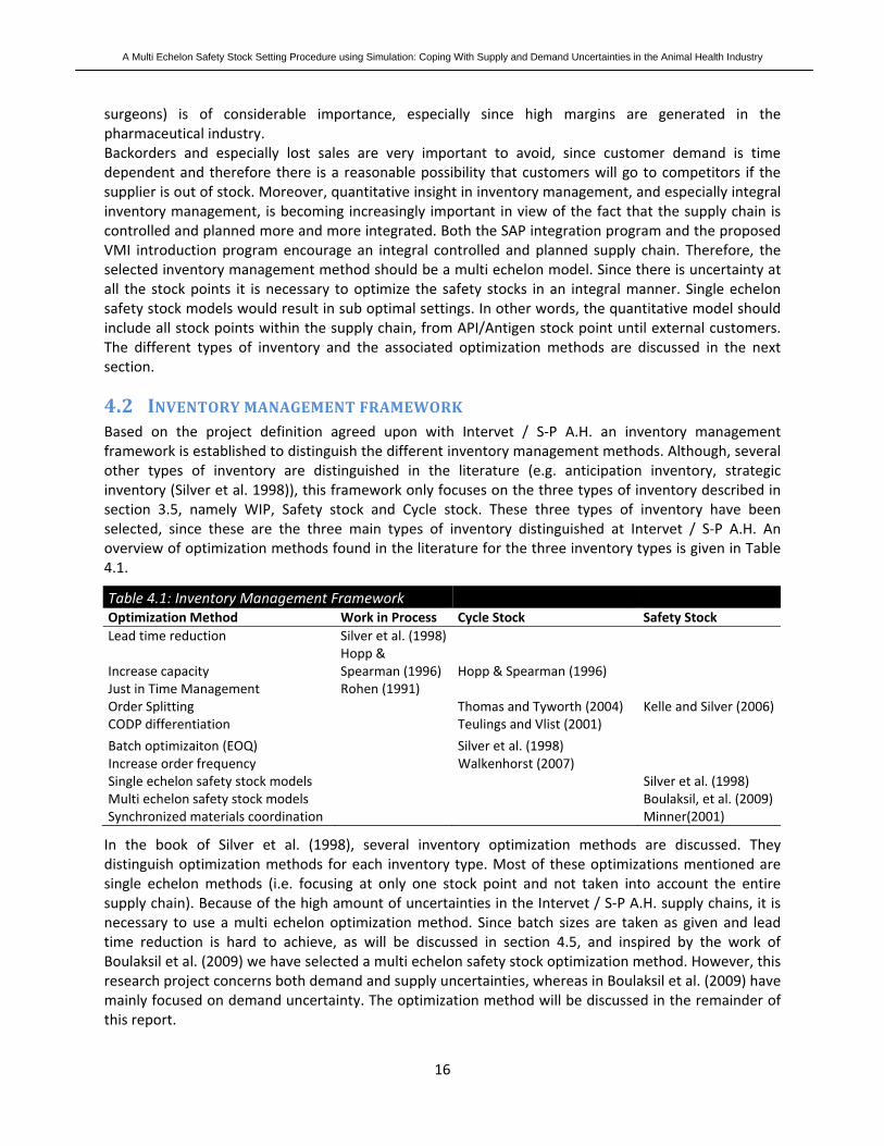
4.2 INVENTORY MANAGEMENT FRAMEWORK Based on the project definition agreed upon with Intervet / S‐P A.H. an inventory management framework is established to distinguish the different inventory management methods. Although, several other types of inventory are distinguished in the literature (e.g. anticipation inventory, strategic inventory (Silver et al. 1998)), this framework only focuses on the three types of inventory described in section 3.5, namely WIP, Safety stock and Cycle stock. These three types of inventory have been selected, since these are the three main types of inventory distinguished at Intervet / S‐P A.H. An overview of optimization methods found in the literature for the three inventory types is given in Table 4.1.
Table 4.1: Inventory Management Framework Optimization Method Work in Process Cycle Stock Safety StockLead time reduction Silver et al. (1998)
Increase capacity Hopp & Spearman (1996) Hopp & Spearman (1996)
Just in Time Management Rohen (1991) Order Splitting Thomas and Tyworth (2004) Kelle and Silver (2006)CODP differentiation Teulings and Vlist (2001)
Batch optimizaiton (EOQ) Silver et al. (1998) Increase order frequency Walkenhorst (2007) Single echelon safety stock models Silver et al. (1998)Multi echelon safety stock models Boulaksil, et al. (2009)Synchronized materials coordination Minner(2001)
In the book of Silver et al. (1998), several inventory optimization methods are discussed. They distinguish optimization methods for each inventory type. Most of these optimizations mentioned are single echelon methods (i.e. focusing at only one stock point and not taken into account the entire supply chain). Because of the high amount of uncertainties in the Intervet / S‐P A.H. supply chains, it is necessary to use a multi echelon optimization method. Since batch sizes are taken as given and lead time reduction is hard to achieve, as will be discussed in section 4.5, and inspired by the work of Boulaksil et al. (2009) we have selected a multi echelon safety stock optimization method. However, this research project concerns both demand and supply uncertainties, whereas in Boulaksil et al. (2009) have mainly focused on demand uncertainty. The optimization method will be discussed in the remainder of this report.
A Multi Echelon Safety Stock Setting Procedure using Simulation: Coping With Supply and Demand Uncertainties in the Animal Health Industry
17
4.3 RESEARCH QUESTION / RESEARCH GOAL Since reaching a feasible service level is of considerable importance in the pharmaceutical industry, as already discussed in section 4.1, we have selected an inventory management method which optimizes the inventory type that is most directly related to the service level reached (i.e. safety stock). Furthermore, it is necessary to conceptualize and quantify the different uncertainty factors described in section 3.4. Therefore, we have selected the multi echelon safety stock model to determine the impact of these uncertainty factors on the service level and the optimal safety stock levels to reach this predefined service level. Based on these arguments and the research gaps in the current literature described briefly in the introduction, the following research question was formulated:
What is the impact of the different uncertainty factors on the safety stock levels and what is the optimal safety stock level at the various stock points to reach the service level against minimal inventory costs?
In line with this research question, the following research goals are formulated: • Develop a quantitative multi echelon safety stock model to determine the optimal safety stock
levels at the controlled stock points for the supply chains in scope • Determine the impact of the various uncertainty factors on the average total inventory • Determine the impact of reducing the uncertainty factors on the average total inventory
Although we are aware of the fact that the heuristic used to find the ‘optimal’ safety stock levels (discussed in chapter 7) will only find an approximation of the optimal safety stock levels, since the optimization process stops although a local optimum might be found, we will use the term optimal safety stock levels throughout this report. In the next section a more detailed description of the research goals and the phase in which they will be realized is given.
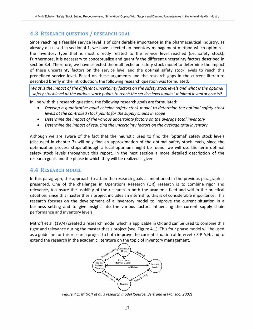
4.4 RESEARCH MODEL In this paragraph, the approach to attain the research goals as mentioned in the previous paragraph is presented. One of the challenges in Operations Research (OR) research is to combine rigor and relevance, to ensure the usability of the research in both the academic field and within the practical situation. Since this master thesis project includes an internship, this is of considerable importance. This research focuses on the development of a inventory model to improve the current situation in a business setting and to give insight into the various factors influencing the current supply chain performance and inventory levels. Mitroff et al. (1974) created a research model which is applicable in OR and can be used to combine this rigor and relevance during the master thesis project (see, Figure 4.1). This four phase model will be used as a guideline for this research project to both improve the current situation at Intervet / S‐P A.H. and to extend the research in the academic literature on the topic of inventory management.
Figure 4.1: Mitroff et al.’s research model (Source: Bertrand & Fransoo, 2002)
A Multi Echelon Safety Stock Setting Procedure using Simulation: Coping With Supply and Demand Uncertainties in the Animal Health Industry
18
Mitroff et al.’s model does not include the orientation phase. Within this additional phase, theoretical background has been used to get familiar with the business processes within the organization. The research proposal has been written during the orientation phase and was the final deliverable of this phase. From here on the four consecutive phases of Mitroff et al’s model will be passed through, starting with the conceptualization phase.
4.4.1 CONCEPTUALIZATION This phase is the first of four consecutive phases within the Mitroff et al.’s research model. Within this phase, the conceptual model of the problem and system under consideration is made. During this phase, there has been decided which variables need to be included in the model. The conceptual model description should use as much as possible concepts and terms that are accepted as standards published in the scientific operations management literature (Bertrand & Fransoo, 2002). In this master thesis project the conceptual phase consists of the determination of the necessary input parameters for the multi echelon safety stock model and the calculation of these parameters for the supply chains in scope. This conceptual model is discussed thoroughly in the next chapter.
4.4.2 MODELING The second phase is the specification of the scientific model of the process or problem. This scientific model must be presented in formal, mathematical terms, such that either mathematical or numerical analysis is possible, or computer simulation can be carried out (Bertrand & Fransoo, 2002). According to Bertrand and Fransoo (2002), quantitative models are based on a set of variables that vary over a specific domain, while quantitative and causal relationships have been defined between these variables. The purpose of this phase is to build the quantitative model. This mainly includes the definition of the variables and parameters used as well as the linkage between the variables. In this particular situation, the quantitative model will be an inventory management optimization model selected from the inventory management framework conducted in the conceptualization phase. More precisely, a multi echelon safety stock model is established. In other words, a simulation model which can be used to determine the influence of various safety stock allocations over the three controlled stock points on the service level is established. Based on the findings during this previous phase, the optimization method which is highly related to the uncertainties described in the supply chain and to the service level defined in the previous phase will be selected. The input parameters described in chapter 5 will be incorporated in the model. The mathematical description of the quantitative model is given in the first part of chapter 6. After establishing the mathematical model, a verification and validation test, described in the last part of chapter 6, will be conducted. These tests are obligatory to start with the model solving phase.
4.4.3 MODEL SOLVING In the third phase, the mathematical algorithms or simulation software required to solve the quantitative model are selected and used to solve the model. Due to the complexity of the biological supply chains in the pharmaceutical industry, as described in the former section, the model or problem might be too complex for formal mathematical analysis. Bertrand en Fransoo (2002), indicate that in case of high complexity, computer simulations are often used instead of mathematical models.
A Multi Echelon Safety Stock Setting Procedure using Simulation: Coping With Supply and Demand Uncertainties in the Animal Health Industry
19
This type of research generally leads to lower scientific quality results than research using mathematical analysis, but the scientific relevance of the process or problem studied may be much higher. However, using simulation software requires a number of additional steps. In this research project, the model solving phase will result in a range of different optimized scenarios for the supply chains within scope. First a structural iterative process of optimization for the supply chains in scope is started to determine the optimal inventory level to reach the feasible service level against minimal cost. An experimental design is established and the impact of the various input parameters on the service level and inventory levels is determined. Moreover, a sensitivity analysis is conducted to determine the impact of changes in the input parameters on the service level. The various scenarios are presented in the first part of chapter 7 and the results are discussed in the last part of chapter 7.
4.4.4 IMPLEMENTATION The implementation phase is the final phase of the research methodology and includes the integration process of the results in the real life situation. However, in this master thesis project the implementation phase will be used to summarize the different scenarios determined in the previous phase in a management presentation and present these scenarios throughout the organization. During this time period the master thesis will be written and management presentations will be given to inform the SCM department about the model and the results. The master thesis project will be finalized during this phase. This phase is described in more detail in chapter 8.
4.5 PROJECT SCOPE This research focuses both on Biological and Pharmaceutical Supply Chains and demand as well as supply uncertainty are incorporated. The different types of uncertainty have been discussed in section 3.4. Supply chains within the manufacturing site of Boxmeer are selected, since this site manufactures a wide range of biologics and manufactures pharmaceuticals as well. In cooperation with Intervet / S‐P A.H. we have selected the pharmaceutical product Pharma product X and the biologics A and B as the products which will be used for the quantitative model. The supply chain structure and characteristics of these supply chains will be discussed in more detail in chapter 5. These products have been selected since there is sufficient data available, there is no seasonal or trend pattern in the demand for these products and are mainly produced in Boxmeer. Since the service level determined will be the service level towards the end customer, the supply chains within scope include the external customers (as visualized in Figure 3.1). This decision has been made, since the service level at this stock point is the best means for measuring customer satisfaction. Batch sizes are fixed in the pharmaceutical industry since they are agreed upon during the registration process of products in the early phase of their life cycle. Therefore this aspect is not within the scope of this master thesis. Moreover, capacity is assumed as given and therefore, the current capacity is used as a restriction during this project. The demand forecast is taken as given as well. Furthermore, WIP, Cycle stock and other stock types are beyond the scope of this research project.

A Multi Echelon Safety Stock Setting Procedure using Simulation: Coping With Supply and Demand Uncertainties in the Animal Health Industry
20
Summarized: - Pharmaceutical and Biological Supply Chains - Boxmeer manufacturing site - From Antigen level until end customer - Focus on Supply Uncertainty (however incorporate Demand Uncertainty) - Demand forecast, capacity and batch sizes are taken as given

A Multi Echelon Safety Stock Setting Procedure using Simulation: Coping With Supply and Demand Uncertainties in the Animal Health Industry
21
5 CONCEPTUAL MODEL (CONCEPTUALIZATION) In this chapter the conceptual model of the problem and system under consideration will be described and there will be decided which variables need to be included in the model. In section 5.1, the structure and main characteristics of the selected supply chains are discussed. The definition of the input parameters for the safety stock model and quantitative analysis to determine the correct values will be discussed in section 5.2.
5.1 SUPPLY CHAINS IN SCOPE As already discussed in chapter 3, we have selected one pharmaceutical supply chain (product Pharma product X) and one biological supply chain (product Bio product Y). The Pharma product X supply chain is less complex, since there are no yield activity fluctuations and furthermore this chain only contains one bulk type. The biological supply chain, on the other hand, contains two antigen which can be used to produce four bulk types. Moreover, part of the biological production process is executed at other production sites than the manufacturing site Boxmeer. The most upstream stage included in the model for the Pharma product X supply chain is the procurement stage of the two APIs. Both APIs are used for the production of the Pharma product X bulk, which are consecutively filled into both the 50 ML and 100 ML FPUs. Afterwards the FPUs are labeled and shipped to the ComOps. For a graphical representation of the network structure, we refer to Appendix III. This network structure only includes the controlled stock points where safety stock is kept. The most upstream stage in the biological supply chain of Bio product Y in this research is the production of both Antigens. Four different bulks can be produced with A and B antigen. The A antigen can be produced in Boxmeer and the manufacturing site in the United Kingdom(UK), the B antigen on the other hand can only be produced in Boxmeer. Three of the bulks are produced and filled in Boxmeer and both antigen from UK and Boxmeer are used for this production process. One of the A bulks is produced at the manufacturing site in Spain and the A Antigen used is shipped from the UK. These four bulks are filled into different presentations and this results in nine different FPUs, which are labeled and subsequently shipped to various ComOps. This network structure, is given in Appendix IV. Although there are several additives(e.g. water, packaging material) used during the various production phases, these are not included in the simulation model. The cost price of these products is considerably low compared to the cost price of the APIs/Antigens, FPUs and FPPs, and leaving these materials outside the scope of the research is therefore of minor impact.
5.2 INPUT PARAMETER DESCRIPTION Within this conceptual model, the input parameters incorporated in the multi echelon safety stock simulation model will be described. For each input parameter it is described why this parameter is a necessary input for the simulation model, how the values are derived and how these parameters will be incorporated in the model. An overview of the values of these parameters for the Pharma product X and Bio product Y supply chains is given in respectively Appendix V and VI. During the orientation phase we have identified, by investigating the supply chain characteristics, four important aspects which are essential during this master thesis project: Supply Uncertainty, Demand Uncertainty, Service level target and Inventory Management Methods (see, Figure 5.1). For inventory management a service level target is necessary as an input for the inventory optimization. Moreover,

A Multi Echelon Safety Stock Setting Procedure using Simulation: Coping With Supply and Demand Uncertainties in the Animal Health Industry
22
demand and supply uncertainty should be determined and incorporated in the model, since these uncertainties are important factors which influence the inventory levels. Finally, inventory management optimization methods (i.e. multi echelon safety stock model) are used as means to reduce costs given the input parameters.
Figure 5.1: four main elements of research model
The inventory management method in this research project is the multi echelon safety stock model which incorporates the various demand and supply uncertainty factors. The working of this model will be discussed in more detail in chapter 6. Several different supply and demand uncertainty input parameters can be distinguished. Moreover, there are several general input parameters (including the service level target which will be discussed in the next subsection). These different input parameters are visualized in Table 5.1.
Table 5.1: Input parameters and variables quantitative model General Variables Demand Uncertainty Supply Uncertainty Bill of Material Demand Forecast Yield Order Quantities Actual Demand Batch rejection MRP Lead times Test repetition Cost parameters Batch output fluctuation Safety stocks Actual Lead times
There will be elaborated on these input parameters and variables in the upcoming sub sections, starting with the general input parameters. Service level is the output of the simulation study and the performance measure. The uncertainty factors are the parameters which will be changed to determine the impact of these parameters and the other general values (e.g. BOM and order quantities) are variables incorporated in the model. Safety stock on the other hand is a parameter in this simulation study.
5.2.1 GENERAL VARIABLES The general variables shown in Table 5.1 are discussed in this sub section. The input values of these variables are given in Appendix VA,B,C,D and VIA,B,C,D Bill of Material(BOM) The Bill of Material is used to determine the supply chain structure and the different controlled stock points in the supply chain. Moreover, the amount of material used to produce the successor of this material. For example, the amount of API to produce a batch of Bulk and FPU is given in the BOM. Furthermore, the factors to translate from one unit of measure to the other is described in the BOM. For example, the unit of measure of FPUs is the amount of vials and the unit of measure for API is Kilograms. The BOMs for the supply chains in scope are given in Appendix VA and VIA.

A Multi Echelon Safety Stock Setting Procedure using Simulation: Coping With Supply and Demand Uncertainties in the Animal Health Industry
23
Order Quantities The order quantities at API/Antigen and FPU level are given and are equal to the fixed batch sizes agreed upon during the registration of the product and production process. For the FPPs, on the other hand, minimal order quantities are used. These minimal order quantities are calculated by using an adjusted EOQ, as already discussed in chapter 3. Both the batch sizes and EOQ values are fixed quantities in the simulation model and used as MRP planning parameters. These values are equal to the order quantities at the controlled stock points. Safety stocks The actual safety stock settings are used to determine the supply chain performance in the current situation. The service level generated when running the simulation with the actual safety stock settings is used to validate the model. In other words, the outcome of the simulation model is compared with the actual service level measured by Intervet / S‐P A.H. Afterwards the safety stock is variable and optimal values are found in an iterative manner to determine the best safety stock allocation over the controlled stock points for the different sub questions discussed in chapter 7. MRP lead times The MRP lead times are used as planning parameters in the reorder point calculation at the controlled stock points. These estimated lead times can be dived into transportation time, quality control time, production time and planning time. These lead times are expected values and therefore only used for the planning process. Cost parameters Two important cost parameters need to be distinguished: cost price and sales price. The former includes material costs and production cost and is necessary to determine the inventory cost at each stock point. Inventory cost are equal to 25% of the cost price. The later is used to determine the total sales volume in dollars, by multiplying the total demand by the sales price. The margin of each FPP can be determined by calculating the difference between sales price and cost price for each FPP. These margins are used in the service level calculation which will be discussed later on. Service level Providing a clearly defined and measurable service level is essential, since at this point in time there is no overall accepted service level at Intervet / S‐P A.H. and a service level is one of the required input parameters for inventory management optimization methods. The following service level definition was established in cooperation with Intervet / S‐P A.H.: The fraction (percentage of margin volume in dollars) of customer demand that is met routinely (i.e. met directly out of stock without backorders or lost sales). Remark: from stock delivery is always on time delivery (i.e. no early and late deliveries in case of sufficient stock) and delivery time from ComOps to customer is not taken into account in service level definition. However, partial deliveries are allowed. The service level will be determined with the following formula (a definition of the symbols is given in Appendix VIII):
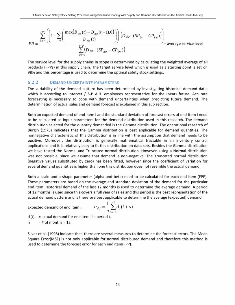
A Multi Echelon Safety Stock Setting Procedure using Simulation: Coping With Supply and Demand Uncertainties in the Animal Health Industry
24
( ) ( )
( )∑
∑ ∑
=
= =
−⋅
⎟⎟
⎠
⎞
⎜⎜
⎝
⎛−⋅⋅⎟
⎟⎠
⎞⎜⎜⎝
⎛⎟⎟⎠
⎞⎜⎜⎝
⎛ −−−
= FPP
fppfppfppfpp
FPP
fppfppfppfpp
T
t fpp
fppfpp
CPSPD
CPSPDtD
tBtB
FR
1
1 1
)(
)()(
0),1()(max1
= average service level
The service level for the supply chains in scope is determined by calculating the weighted average of all products (FPPs) in this supply chain. The target service level which is used as a starting point is set on 98% and this percentage is used to determine the optimal safety stock settings.
5.2.2 DEMAND UNCERTAINTY PARAMETERS The variability of the demand pattern has been determined by investigating historical demand data, which is according to Intervet / S‐P A.H. employees representative for the (near) future. Accurate forecasting is necessary to cope with demand uncertainties when predicting future demand. The determination of actual sales and demand forecast is explained in this sub section. Both an expected demand of end‐item i and the standard deviation of forecast errors of end‐item i need to be calculated as input parameters for the demand distribution used in this research. The demand distribution selected for the quantity demanded is the Gamma distribution. The operational research of Burgin (1975) indicates that the Gamma distribution is best applicable for demand quantities. The nonnegative characteristic of this distribution is in line with the assumption that demand needs to be positive. Moreover, the distribution is generally mathematical tractable in an inventory control applications and it is relatively easy to fit this distribution on data sets. Besides the Gamma distribution we have tested the Normal and Truncated normal distribution. However, using a Normal distribution was not possible, since we assume that demand is non‐negative. The Truncated normal distribution (negative values substituted by zero) has been fitted, however since the coefficient of variation for several demand quantities is higher than one this distribution does not resemble the actual demand. Both a scale and a shape parameter (alpha and beta) need to be calculated for each end item (FPP). These parameters are based on the average and standard deviation of the demand for the particular end item. Historical demand of the last 12 months is used to determine the average demand. A period of 12 months is used since this covers a full year of sales and this period is the best representation of the actual demand pattern and is therefore best applicable to determine the average (expected) demand.
Expected demand of end item i: ∑−
−=
+=1
, )(1ns
iid stdn
μ
di(t) = actual demand for end item i in period t. n = # of months = 12 Silver et al. (1998) indicate that there are several measures to determine the forecast errors. The Mean Square Error(MSE) is not only applicable for normal distributed demand and therefore this method is used to determine the forecast error for each end item(FPP).

A Multi Echelon Safety Stock Setting Procedure using Simulation: Coping With Supply and Demand Uncertainties in the Animal Health Industry
25
Forecast errors: MSEi(h) = ( )∑−
−=
+−+−+1 2
),(ˆ)(1Ts
ii sthstdstdT
T = length of planning horizon, being equal to 12 months di(t‐h,t) = forecast made in period t – h for demand in period t of end item i. h = equal to 6 months The forecast horizon(h) is fixed and equal to 6 months. Therefore, the forecast estimated 6 months in advance is used to determine the forecast error. We have selected a 6 months horizon, since Intervet / S‐P A.H. is currently using an average of forecast errors with a forecast horizon of 3, 6 and 9 months. The length of the planning horizon(T) is equal to 12 months, which indicates that the last 12 months (year) of sales is used to determine the MSE value.
The id ,σ can be calculated using the following formula: iid MSE=,σ (Silver et al., 1998).The square
root is used to convert the forecast error values to the standard deviation. Since these demand parameters are currently measured on a monthly basis and planning is updated every week, it is necessary to change the values of these parameters into a weekly average and a weekly standard
deviation. This has been done by respectively dividing id ,μ by 30/7 and id ,σ by √(30/7). This method is
similar to the method used by Intervet / S‐P A.H. and since the simulation model resembles the planning model of Intervet / S‐P A.H. we have used the same method to calculate the weekly demand. Thereafter, the scale and shape parameter of the Gamma distribution can be estimated as follows (Burgin, 1975):
Alpha =
7/30
7/302
,
2,
id
id
i σ
μ
α = Beta =
7/30
7/30,
2,
id
id
i μ
σ
β =
Actual Demand The actual sales will be generated each week for each end item and will be a random value from the Gamma distribution with the calculated scale and shape parameter. An overview of the scale and shape parameters for the different FPPs for the supply chains in scope is given in section 5.3. Demand forecast The forecast will be a stationary forecast with a value equal to the average demand during the last 12
months of historical demand data: id ,μ . In other words, the demand forecast for the products will be
constant over time and have an equal value each week. This is agreed upon since the forecast calculated by Intervet / S‐P A.H. for the selected products is relatively flat as well and this therefore fairly resembles the current situation at Intervet / S‐P A.H. Forecast Accuracy The average forecast accuracy (FA) has been calculated by first calculating the average forecast accuracy per time period for each end item (FPP). This has been done by calculating the absolute difference between the actual demand in period t )(tX fpp and the forecasted demand fppμ and subsequently
dividing this absolute value by the forecasted demand. Afterwards the average value over the entire simulation length is taken to determine the average forecast accuracy per end item.
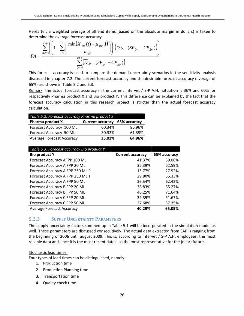
A Multi Echelon Safety Stock Setting Procedure using Simulation: Coping With Supply and Demand Uncertainties in the Animal Health Industry
26
Hereafter, a weighted average of all end items (based on the absolute margin in dollars) is taken to determine the average forecast accuracy.
( ) ( )
( )∑
∑ ∑
=
= =
−⋅
⎟⎟
⎠
⎞
⎜⎜
⎝
⎛−⋅⋅⎟
⎟⎠
⎞⎜⎜⎝
⎛⎟⎟⎠
⎞⎜⎜⎝
⎛ −−
= FPP
fppfppfppfpp
FPP
fppfppfppfpp
T
t fpp
fppfpp
CPSPD
CPSPDtX
FA
1
1 1
)(
)(1,)(min
1μ
μ
This forecast accuracy is used to compare the demand uncertainty scenarios in the sensitivity analysis discussed in chapter 7.2. The current forecast accuracy and the desirable forecast accuracy (average of 65%) are shown in Table 5.2 and 5.3. Remark: the actual forecast accuracy in the current Intervet / S‐P A.H. situation is 36% and 60% for respectively Pharma product X and Bio product Y. This difference can be explained by the fact that the forecast accuracy calculation in this research project is stricter than the actual forecast accuracy calculation.
Table 5.2: Forecast accuracy Pharma product X Pharma product X Current accuracy 65% accuracy Forecast Accuracy 100 ML 60.34% 86.96%Forecast Accuracy 50 ML 30.92% 61.39%Average Forecast Accuracy 35.01% 64.96% Table 5.3: Forecast accuracy Bio product Y Bio product Y Current accuracy 65% accuracy Forecast Accuracy AFPP 100 ML 41.37% 59.06% Forecast Accuracy A FPP 20 ML 35.39% 62.59% Forecast Accuracy A FPP 250 ML P 13.77% 27.92% Forecast Accuracy A FPP 250 ML T 29.80% 55.33% Forecast Accuracy A FPP 50 ML 36.54% 62.42% Forecast Accuracy B FPP 20 ML 38.83% 65.27% Forecast Accuracy B FPP 50 ML 46.25% 71.64% Forecast Accuracy C FPP 20 ML 32.39% 51.67% Forecast Accuracy C FPP 50 ML 27.68% 57.35% Average Forecast Accuracy 40.29% 65.05%
5.2.3 SUPPLY UNCERTAINTY PARAMETERS The supply uncertainty factors summed up in Table 5.1 will be incorporated in the simulation model as well. These parameters are discussed consecutively. The actual data extracted from SAP is ranging from the beginning of 2006 until august 2009. This is, according to Intervet / S‐P A.H. employees, the most reliable data and since it is the most recent data also the most representative for the (near) future. Stochastic lead times: Four types of lead times can be distinguished, namely:
1. Production time
2. Production Planning time
3. Transportation time
4. Quality check time

A Multi Echelon Safety Stock Setting Procedure using Simulation: Coping With Supply and Demand Uncertainties in the Animal Health Industry
27
All these lead times have been expressed in calendar days to make sure that calculations are done correctly. For each of these times a distribution has been fitted which is used as the actual lead time for the various phases. The distribution is fitted on the actual data retrieved by using Every Angle, which is an add on for SAP and is an useful tool to extract data from SAP. The add on for Microsoft Excel named @Risk is used to determine the best fitting distribution functions for these lead times. However, when there is no fitting distribution function, an empirical distribution is used and there will be randomly drawn from this distribution (which is an option in the simulation software used). An overview of the distributions used for the different lead times is shown in Appendix VF and VIF. Besides the distribution functions shown in Appendix VF and VIF, there are lead times for which no distribution could be fitted. Therefore, we have chosen the empirical distribution for the process times of Bulk, FPU and FPP. Moreover, the transportation time for FPPs from manufacturing site to ComOps is taken as deterministic with a value equal to the MRP parameter value since for most of the ComOps (i.e. those ComOps which are not on SAP) there is no actual data for the transportation times available and the values for transportation times for the SAP ComOps are relatively constant. Yield An important uncertainty factor, mainly in biological supply chains, is the yield uncertainty. Nahmias (2005) indicates that this yield uncertainty results from imperfect production processes. Recommendations to incorporate this yield uncertainty in the MRP planning are adjusting the scrap allowance (Nahmias, 2005) or the safety stock (Silver et al., 1998). The yield uncertainty is determined by calculating the actual yield factor (i.e. the activity factor of a particular Antigen batch) and determine the difference (in percentage of the expected yield factor) of each batch compared to the expected yield factor (i.e. the proportion unit, which is the standard activity used as planning parameter in MRP). These values are calculated and determined after the quality inspection of the Antigens. The yield fluctuation is drawn from an empirical distribution (i.e. yield values are randomly drawn from the yield fluctuations data set). Average yield values are given in Appendix VIE. Batch value deviations Besides the yield uncertainty for the biological Antigens, there is a quantity difference between the target quantity and the actual quantity of each batch produced. During the production process, there might be a loss of material which results in a lower batch quantity and therefore there is a batch value deviation. This deviation is determined in the same manner as the yield uncertainty factor and given in Appendix VE and VIE. Test repetition After the quality test there might be indicated that one of the tests needs to be redone, because certain test values fall outside the specifications. This might indicate that there are problems with the quality of the batch or with the validity of the test. Therefore, a test resulting in values outside the specifications will be repeated. This parameter is incorporated by including a percentage of test repetition after the main quality inspections at the API/Antigen and FPU stock points. This parameter is calculated by determining the percentage of the total number of batches at each stock point which are retested. A binominal distribution with the calculated percentage is used to determine whether a batch should be retested. The binominal distribution is the best fitting distribution, since the data indicates that a certain percentage of the tests needs to be redone. Retests do not occur in the Pharma product X supply chain, however there are tests redone in the Bio product Y supply chain at Antigen and FPU level. The percentage of test repetition for the Biological supply chain is given in Appendix VIE.

A Multi Echelon Safety Stock Setting Procedure using Simulation: Coping With Supply and Demand Uncertainties in the Animal Health Industry
28
Batch rejection When quality inspections indicate that there is a serious problem with the quality of a certain batch, it might be necessary to reject the whole batch or in some cases part of the batch. This is of considerable importance for the planning process, since this is an unexpected loss of a (sub) batch. A percentage of batch rejections is determined in the same manner as the test repetition percentage. Moreover, the binominal distribution is used for this input parameters as well. The reasoning for using the binominal distribution is similar to the reasoning described for test repetition. These batch rejections only occur at the FPU and API/Antigen stock points. The percentage of batch rejections at each stock point is given in Appendix VE and VIE.

A Multi Echelon Safety Stock Setting Procedure using Simulation: Coping With Supply and Demand Uncertainties in the Animal Health Industry
29
6 SIMULATION MODEL (CONCEPTUALIZATION) In this chapter, the design of the simulation model used to determine the impact of various safety stock allocations over the three controlled stock points on the service level for the different sub questions is given. Section 6.1 discusses the assumptions of the safety stock model. The working of the simulation model is described in section 6.2. In section 6.3, the validation and verification of the model is described.
6.1 MODEL ASSUMPTIONS This section presents the assumptions made in this simulation study. The assumptions indicate which aspects are taken into account and which aspects are beyond the scope of the simulation model. Assumptions
General - The model considers the total supply chain, i.e. it should be a multi‐echelon model, containing
the three controlled stock points shown in Figure 6.1. - Shortages are backordered and will be delivered the first period when inventory is available - Partial deliveries are possible from FPP to customer and from FPU to FPP - From API/Antigen to Bulk and Bulk to FPU there are no partial deliveries - Batch sizes are registered and therefore fixed at the API/Antigen, Bulk and FPU stock point. - Planning will be updated on a weekly basis(time bucket = one week) - Order Quantities / Batch sizes are given - Resource capacity is non restricting - Safety stocks are integer values Demand - Demand quantities are gamma distributed - There is no trend or seasonal pattern in demand - Forecast error is based on forecast 6 months before actual sales - End items (FPPs) are arranged based on decreasing revenue margin and demand of end items
with highest margin is fulfilled first
6.2 SIMULATION MODEL DESIGN A combination of the various uncertainty factors, discussed in chapter 5, results in increased modeling complexity. Bertrand en Fransoo (2002), indicate that in case of high complexity, computer simulations are often used instead of mathematical models. Therefore, we have decided to establish a simulation model to conduct this research. The simulation model reflects the companies’ planning process and since Material Requirements Planning(MRP) is used as the planning tool at Intervet / S‐P A.H. it is necessary to utilize the MRP logic in the simulation model. The simulation program Arena 12.0 is used as the modeling tool because of the ease in usability (i.e. relatively easy for output gathering and analysis). The simulation model uses the constant MRP planning data used at Intervet / S‐P A.H. to determine the reorder points at the three controlled stock points. Moreover, various distributions are used to model the actual lead times and other uncertainties in this simulation model. The MRP planning data and actual lead time averages and distributions are shown in Appendix VF and VIF. We will simulate the supply chain of one pharmaceutical product group (Pharma product X) and two biological product groups (A and B).

A Multi Echelon Safety Stock Setting Procedure using Simulation: Coping With Supply and Demand Uncertainties in the Animal Health Industry
30
The three main process (i.e. FPP, FPU and API/Antigen) will be discussed separately in the remainder of this section and are visualized in Figure 6.1 . The definition of the symbols used in this section are given in Appendix VIII.
Figure 6.1: three controlled stock points in simulation model
Since we want to perform a stationary simulation, it is necessary to determine a warm up period. This warm up period is the simulation time required to achieve a steady state condition. A steady state simulation implies that a simulation has reached a point in time where the state of the simulation is independent of the initial start‐up conditions. Besides the warm up period, it is also necessary to determine the run length and the number of replications. A description of the determination of these parameters is given in Appendix IX. Object function The objective of this simulation model is to minimize the Average Total Inventory cost in the total supply chain, while reaching the desired service level and given the MRP logic. This objective is reached by changing the safety stock values at the three controlled stock points. Safety stock is used as the input variable in this model and two other types of inventory, namely Work in Process (Quality stock) and Physical Inventory (Released stock) are recorded and used as output variables in this simulation model. The Total Inventory is the Physical Inventory plus the Work In Process. This leads to the following objective function:
( ) ( ) ( )⎟⎟⎠
⎞⎜⎜⎝
⎛⋅++⋅++⋅+ ∑∑∑
===
RM
rmrmrmrm
FPU
fpufpufpufpu
FPP
fppfppfppfpp CPPIWIPCPPIWIPCPPIWIP
111
)()()(min (1)
The average Work In Process and average Physical Inventory at the three controlled stock points can be calculated by using formula (2) and (3).
T
tWIPWIP
T
tfpp
fpp
∑== 1
)(
T
tWIPWIP
T
tfpu
fpu
∑== 1
)(
T
tWIPWIP
T
trm
rm
∑== 1
)( (2)
T
tPIPI
T
tfpp
fpp
∑== 1
)(
T
tPIPI
T
tfpu
fpu
∑== 1
)(
T
tPIPI
T
trm
rm
∑== 1
)( (3)
Performance measure To determine the overall service level (i.e. fill rate), which is the performance measure used in this model, first the service level of each individual FPP has been calculated. This has been done by dividing the total incremental amount of back orders by the total demand over all simulation periods. One minus this value is the service level of this end item. We have determined the weighted average of the individual fill rates to determine the overall fill rate. The service level used to calculate the service level of the supply chains in scope is determined with formula 4. On average, the FPPs with higher revenue margins will perform better, since the FPPs are arranged based on revenue margin in a decreasing order and delivering the demand of FPPs with high margin has a higher priority than demand of other FPPs. Eventually, this results in a higher average performance.
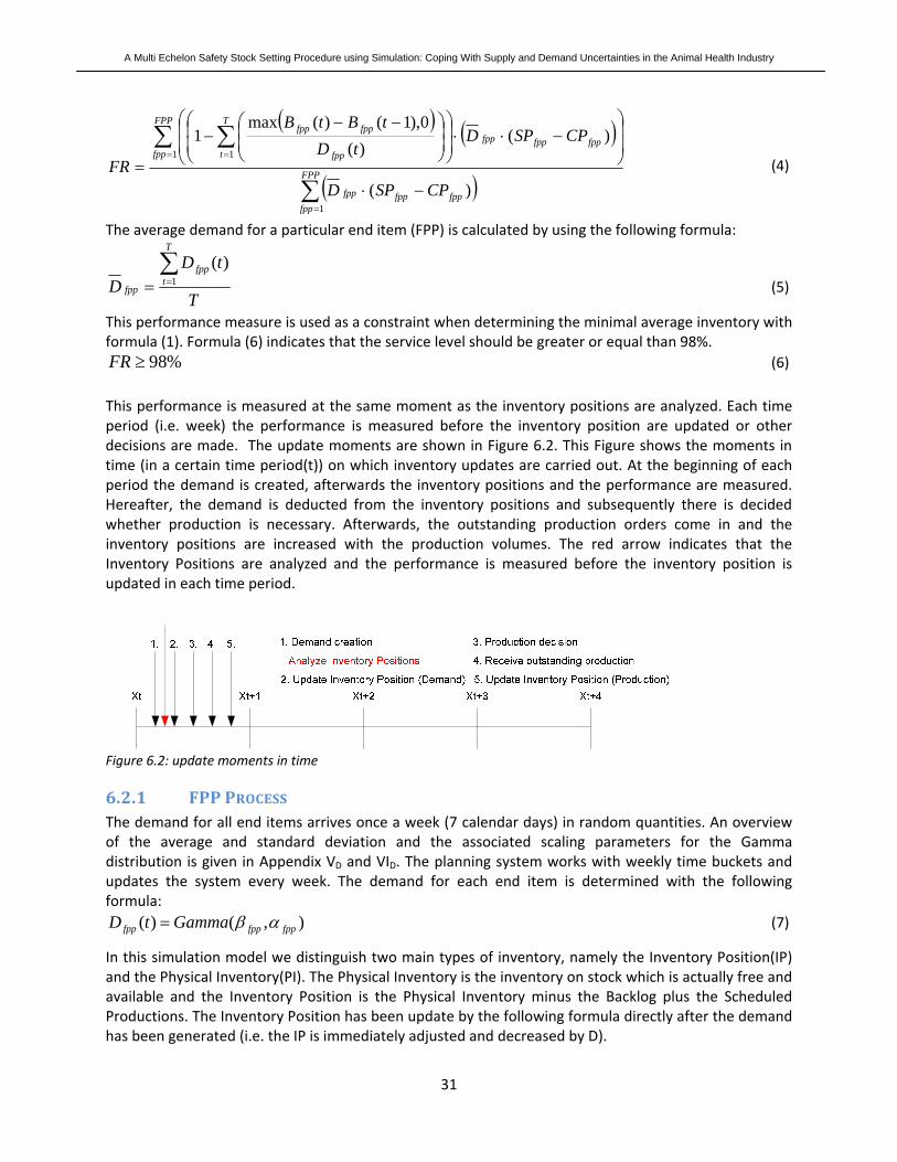
A Multi Echelon Safety Stock Setting Procedure using Simulation: Coping With Supply and Demand Uncertainties in the Animal Health Industry
31
( ) ( )
( )∑
∑ ∑
=
= =
−⋅
⎟⎟
⎠
⎞
⎜⎜
⎝
⎛−⋅⋅⎟
⎟⎠
⎞⎜⎜⎝
⎛⎟⎟⎠
⎞⎜⎜⎝
⎛ −−−
= FPP
fppfppfppfpp
FPP
fppfppfppfpp
T
t fpp
fppfpp
CPSPD
CPSPDtD
tBtB
FR
1
1 1
)(
)()(
0),1()(max1
(4)
The average demand for a particular end item (FPP) is calculated by using the following formula:
T
tDD
T
tfpp
fpp
∑== 1
)( (5)
This performance measure is used as a constraint when determining the minimal average inventory with formula (1). Formula (6) indicates that the service level should be greater or equal than 98%.
%98≥FR (6) This performance is measured at the same moment as the inventory positions are analyzed. Each time period (i.e. week) the performance is measured before the inventory position are updated or other decisions are made. The update moments are shown in Figure 6.2. This Figure shows the moments in time (in a certain time period(t)) on which inventory updates are carried out. At the beginning of each period the demand is created, afterwards the inventory positions and the performance are measured. Hereafter, the demand is deducted from the inventory positions and subsequently there is decided whether production is necessary. Afterwards, the outstanding production orders come in and the inventory positions are increased with the production volumes. The red arrow indicates that the Inventory Positions are analyzed and the performance is measured before the inventory position is updated in each time period.
Figure 6.2: update moments in time
6.2.1 FPP PROCESS The demand for all end items arrives once a week (7 calendar days) in random quantities. An overview of the average and standard deviation and the associated scaling parameters for the Gamma distribution is given in Appendix VD and VID. The planning system works with weekly time buckets and updates the system every week. The demand for each end item is determined with the following formula:
),()( fppfppfpp GammatD αβ= (7)
In this simulation model we distinguish two main types of inventory, namely the Inventory Position(IP) and the Physical Inventory(PI). The Physical Inventory is the inventory on stock which is actually free and available and the Inventory Position is the Physical Inventory minus the Backlog plus the Scheduled Productions. The Inventory Position has been update by the following formula directly after the demand has been generated (i.e. the IP is immediately adjusted and decreased by D).
A Multi Echelon Safety Stock Setting Procedure using Simulation: Coping With Supply and Demand Uncertainties in the Animal Health Industry
32
)()(:)( tDtIPtIP fppfppfpp −= (8)
Hereafter, a check is performed whether the demanded quantity is larger than the Physical Inventory (Dfpp > PIfpp). If this is true, the PI is shipped resulting in a physical inventory equal to zero. The remainder of the demanded quantity is backlogged. If Dfpp ≤ PIfpp, the PI is decreased by the quantity demanded (formula (12)).
)()( tPItQS fppfpp = (9)
0)( =tPI fpp (10)
)()()(:)( tQStDtBtB fppfppfppfpp −+= (11)
)()(:)( tDtPItPI fppfppfpp −= (12)
Now it is determined if production is needed. The following formula is used to check whether production is necessary:
LTfppfppfpp DSStIP +≤)( (13)
The demand during the lead time is calculated by multiplying the average demand per week by 1/7 and then multiplied by the fixed lead time parameters(expressed in calendar days) in MRP.
)(71
fppfppfppfppiLTfpp PLTTTQTPTDD +++⋅⋅= (14)
If (8) is true, the inventory needs to be increased and production is started. Before production starts it is checked whether the Physical Inventory at the preceding stock point (i.e. FPU stock point) is sufficient to produce the order quantity required at the FPP level. This is done by using the following formula for each FPP:
)()( tQtPI fppfpu ≥ (15)
The Qfpp(t) value is zero for those FPPs which do not need additional inventory and equal to
NnQn fpp ∈⋅ , , for those FPPs who do need additional inventory to increment the inventory position to
the desired level. The list of order quantities is given in Appendix VD and VID. The Actual Order Quantity (AOQ) is used to determine the actual amount of FPPs which is produced and depends on the amount of inventory at the FPU. This value is calculated by using formula (16). The FPPs are arranged based on revenue margin in decreasing order and therefore the FPPs gaining the highest revenue are produced first. By using this allocation mechanism, the backorder volume is minimized.
))(),(min()( tQtPItAOQ fppfpufpp = (16)
Hereafter, the Inventory Position at FPP level is immediately increased with AOQ (formula (17)). This process has been repeated for all the FPPs and therefore we have checked whether production is necessary for each FPP at the beginning of each week.
)()(:)( tAOQtIPtIP fppfppfpp += (17)
The following formulas will be used to update the Inventory Position, Physical Inventory and Backlog at the FPU level.
)()(:)(1
tQtIPtIPFPP
fppfppfpufpu ∑
=
−= (18)
A Multi Echelon Safety Stock Setting Procedure using Simulation: Coping With Supply and Demand Uncertainties in the Animal Health Industry
33
∑=
−=FPP
fppfppfpufpu tAOQtPItPI
1)()(:)( (19)
∑∑==
−+=FPP
fppfpp
FPP
fppfppfpufpu tAOQQtBtB
11)()(:)( (20)
The orders or part of the orders which were not produced because of the lack of inventory at the FPU level are stored as outstanding orders. The amount of outstanding orders for each FPP in each time period is calculated by formula (21). The sum of the outstanding orders at the FPP level is equal to the Backlog amount at the FPU level.
)()()(:)( tAOQtQtOOtOO fppfppfppfpp −+= (21)
Those outstanding orders are released when the FPU inventory is greater than zero again. This happens when the FPU production has finished and the FPU inventory level is increased by the order quantity. The Quantity Used for these outstanding orders is calculated with the following formula:
))(),(min()( tBtPItQU fpufpufpu = (22)
The amount of FPU Backlog and FPP outstanding orders is reduced by the Quantity Used. When the FPU Physical Inventory is greater than the FPU Backlog, all outstanding orders will be produced and the amount of Outstanding orders and the FPU Backlog will be equal to zero. The remainder of the Outstanding Orders is stored again, in case the FPU Backlog is greater than the Physical Inventory. This is calculated by using formula (23). The AOQ for the released outstanding orders is equal to the outstanding order amount (formula (24)). Moreover, the Physical Inventory and Backlog amount at the FPU level are decreased by using formula (25) and (26).
))()(,0max(:)( tQUtOOtOO fpufppfpp −= (23)
)()( tOOtAOQ fppfpp = (24)
)()(:)( tQUtPItPI fpufpufpu −= (25)
)()(:)( tQUtBtB fpufpufpu −= (26)
Thereafter, the production process starts for those FPPs which need additional inventory. This process consists of two subsequent steps at the manufacturing site: the actual production (labeling) process and the production planning. Thereafter, the products are transported to the Commercial Operations and finally a local quality control process will take place. An overview of the distributions and averages of the lead times is given in Appendix VF and VIF. After the production process has finished the Physical Inventory is updated by the following formula:
)()(:)( tAOQtPItPI fppfppfpp += (27)
Production can be finished at any moment within each time period, since the production times can be any positive integer number of days. However, planning is updated on a weekly basis and therefore the total production time in days will be rounded off to the nearest integer number of weeks and the production will be available at the beginning of this week (e.g. when the total production time is equal to 25 days, the production will be available at the beginning of week 4). After the physical inventory is increased with the AOQ, it is checked whether any Backlog has to be shipped. The Backlog can be greater than the new available PI since demand can occur during the production time.
A Multi Echelon Safety Stock Setting Procedure using Simulation: Coping With Supply and Demand Uncertainties in the Animal Health Industry
34
When this demand is greater than the sum of the Order Quantity and Physical Inventory before production, not all Backlog can be shipped. This Backlog is therefore checked with the PI and the minimum of the two is used. Thereafter, the Physical Inventory and Backlog are decreased by the Quantity Used.
))(),(min()( tBtPItQU fppfppfpp = (28)
)()(:)( tQUtPItPI fppfppfpp −= (29)
)()(:)( tQUtBtB fppfppfpp −= (30)
6.2.2 FPU PROCESS Demand at the FPU level is the demand derived from FPP. This demand will be deducted from the Inventory at FPU level directly when production at FPP is necessary. The Inventory Position, Physical Inventory and Backlog are updated by using formula (18), (19) and (20). Similar as at the FPP level, at FPU level there has been determined each week whether production is needed. The following formula is used to check whether production is necessary at the FPU level:
LTfpufpufpu DSStIP +≤)( (31)
The demand during the lead time is calculated by multiplying the average demand per week by 1/7 and then multiplied by the fixed lead time parameters in MRP.
)(71
1fpufpufpu
FPP
fppfpp
LTfpu QTPTPLTDD ++⋅⋅= ∑
=
(32)
If (31) is true the inventory needs to be increased and production is started. Before production starts it is checked whether the Physical Inventory at the preceding stock point (i.e. API/Antigen level) is sufficient to produce the order quantity required at the FPU level. Since there are no partial deliveries from API/Antigen stock point to the FPU stock point it is only possible to start FPU production when there is sufficient API/Antigen available. Therefore, formula (34) and (35) are used when respectively there is sufficient API/Antigen and there is not sufficient API/Antigen. Whether there is sufficient API/Antigen to produce a full batch is checked by using formula (33).
rmfpurm BFAPQPI ⋅≥ (33)
)()( tQtAOQ fpufpu = (34)
0)( =tAOQfpu (35)
Since, the batch size of some of the FPUs is smaller than the Bulk batch size and the total Bulk volume always needs to be filled into FPUs it is sometimes necessary to fill the remainder of the Bulk into another FPU presentation (e.g. part of the Bulk in 20 ML FPU and the rest in 50 ML FPU vials). This remainder part is calculated by using the following formula:
( )fpu
fpufpufpufpu BF
BFtAOQAPQtROQ ')()(
⋅−= (36)
The BOM factors(BF) indicate the amount of Bulk necessary for a fixed amount of FPU vials. An overview of the BOM Factors for all the FPUs is given in Appendix VA and VIA. In case the Bulk order quantity is equal to the FPU order quantity, the rest order quantity(ROQ) is equal to zero. When there are more possible FPUs to fill the remainder of the Bulk, there is checked which FPU (which can be produced with this Bulk) has the lowest Inventory Position at the moment the production planning starts.

A Multi Echelon Safety Stock Setting Procedure using Simulation: Coping With Supply and Demand Uncertainties in the Animal Health Industry
35
In other words, the model compares the Inventory Positions of the remaining FPUs using the same Bulk as the Bulk produced and allocates the remaining Bulk to the FPU production process of the FPU with the lowest Inventory Position. The Actual Production Quantity is equal to the Order Quantity of the Bulk, since the production process is restricted by the registered Bulk batch size. The amount of API/Antigen necessary for the production of a FPU batch is equal to the Actual Production Quantity plus the Fixed Quantity, which is used as a start up amount for the Bulk production process. The values of these fixed quantities are given in Appendix VA and VIA.
bulkfpu QAPQ = (37)
bulkfpufpu FQAPQARQ +=
(38)
If formula (33) holds, and therefore there is sufficient inventory at the API/Antigen level, the Inventory Position of the FPU which demanded additional inventory will be updated by using formula (39). The Inventory Position of the other FPU will be updated by using formula (40), in case there is still Bulk material available after the production of the other FPU batch.
)()(:)( tAOQtIPtIP fpufpufpu += (39)
)()(:)( tROQtIPtIP fpufpufpu += (40)
Moreover, the Inventory Position and Physical Inventory at the API/Antigen levels are decreased by using formula 41 and 42.
rmfpurmrm BFARQtIPtIP ⋅−= )(:)( (41)
rmfpurmrm BFARQtPItPI ⋅−= )(:)( (42)
rmfpurmrm BFARQtBtB ⋅+= )(:)( (43)
If formula (33) does not hold, this indicates that there is not sufficient inventory at the API/Antigen level and the prospected order should be backordered. The inventory positions of the FPUs are increased by using formula (39) and (40). However, the orders which were not produced because of insufficient API/Antigen inventory are stored as outstanding orders. The amount of outstanding orders at the FPU level is updated by using formula (44). Furthermore, the Inventory Position and Backlog at the API/Antigen levels are updated by using formula (41) and (43).
)()(:)( tQtOOtOO fpufpufpu += (44)
These outstanding orders remain stored until the API/Antigen inventory is sufficiently high to produce at least one batch of FPU (which has been checked by using formula (33)). The amount of orders released is determined by using formula (45). Thereafter, the outstanding orders at the FPU level and the Physical Inventory and Backlog at the API/Antigen level are updated by using respectively formula (46), (47) and (48).
⎟⎟⎠
⎞⎜⎜⎝
⎛=
)()(
),(min)(tBFtPI
tOOtORrm
rmfpufpu (45)
)()(:)( tORtOOtOO fpufpufpu −= (46)
( ))()()(:)( tBFtORtPItPI rmfpurmrm ⋅−= (47)
( ))()()(:)( tBFtORtBtB rmfpufrmrm ⋅−= (48)

A Multi Echelon Safety Stock Setting Procedure using Simulation: Coping With Supply and Demand Uncertainties in the Animal Health Industry
36
A part of the amount of outstanding orders will not be released, when the amount of inventory available at the API/Antigen level is insufficient to reduce the total amount of outstanding orders. These orders will wait until the inventory at the API/Antigen level will be increased again. The other orders will be produced directly when they are released.
Now the actual production process starts. This process consists of two separate processes. The Bulk production process where API/Antigen is used to produce Bulk and the filling process where this Bulk is filled into vials. The Bulk process consists of a production planning process a production process and a small quality test afterwards. The Filling process consist of a planning process, the actual filling and afterwards two quality tests are executed in parallel. The distribution and the average of these lead times is given in Appendix VF and VIF. After the filling process a deviation of the expected actual order quantity can exist. These deviations are calculated by using formula (49) and (50). The Dv values are the deviations from the expected actual order quantities and are drawn from an empirical distribution which are read from excel.
))(1()()( tDvtAOQtAOQ fpufpuDfpu +⋅= (49)
))(1()()( tDvtROQtROQ fpufpuDfpu +⋅= (50)
After the quality control there is a possibility that a test needs to be redone and this results in additional quality time. This retest can be done for several times and will be repeated with a certain percentage. Moreover, a certain percentage of the batches will be rejected. When a batch is rejected, the inventory position at the FPU level is been updated again by the following formulas:
)()(:)( tAOQtIPtIP Dfpufpufpu −= (51)
)()(:)( tROQtIPtIP Dfpufpufpu −= (52)
When the batch has not been rejected, the FPU process is finished and the PI at FPU level can be updated by the following formula (53) and (54). After the Physical Inventory has been increase with the AOQ, there has been checked whether any outstanding Backlog has to be shipped. This is the Quantity Used value which has already been discussed in sub section 6.2.1 in formula 22, 25 and 26.
)()(:)( tAOQtPItPI Dfpufpufpu += (53)
)()(:)( tROQtPItPI Dfpufpufpu += (54)
6.2.3 API/ANTIGEN PROCESS Demand at the API/Antigen level is the derived demand from FPU and therefore indirectly derived from FPP as well. This demand will be de deducted from the Inventory at API/Antigen level directly when production at FPU is necessary. The Inventory Position and Physical Inventory at the API/Antigen level are decreased by using formula (41) and (42) when there is sufficient inventory and the Backlog and Inventory Position at the API/Antigen level are updated by using (41) and (43) when there is insufficient inventory at the moment when a batch of one of the FPUs needs to be produced. Thereafter, it is checked whether production is needed. The APIs are transported instead of produced, since they are bought from an external supplier. For the Antigens, on the other hand, this is a production process. Formula (55) is used to check whether production is necessary. The demand during the lead time can be calculated with the formula (56) and (57) for API and Antigen respectively.
A Multi Echelon Safety Stock Setting Procedure using Simulation: Coping With Supply and Demand Uncertainties in the Animal Health Industry
37
LTrmrmrm DSStIP +≤)( (55)
rmfpu
FPP
fppfpp
rmrmLTrm BFBFD
TTQTD ⋅⋅⎟⎟
⎠
⎞⎜⎜⎝
⎛⋅
+= ∑
=17 (56)
rmfpu
FPP
fppfpp
rmrmLTrm BFBFD
PTQTD ⋅⋅⎟⎟
⎠
⎞⎜⎜⎝
⎛⋅
+= ∑
=17 (57)
If this is true, then production is needed and first the inventory position is updated by using formula (58).
)()(:)( tQtIPtIP rmrmrm += (58)
Thereafter, the production process starts. This process contains a transportation phase and a quality control phase for APIs and a production phase and a quality phase for Antigens. Since there are batch value deviations in the Antigen production process, the inventory position of the Antigen needs to be updated after the production phase. This is done by using formulas (59) and (60).
))(1()()( tDvtQtAOQ rmrmrm +⋅= (59)
)()()(:)( tAOQtQtIPtIP rmrmrmrm +−= (60)
Antigens can be retested and this will be necessary for a predetermined percentage of the Antigens. Batch rejection is possible for both APIs and Antigens after the final quality check is executed. A percentage of the batches will be rejected and for these batches, the Inventory Position needs to be updated by using formula (61).
)()(:)( tAOQtIPtIP rmrmrm −= (61)
Finally there could be a yield fluctuation which becomes obvious after the final quality check as well. The yield fluctuation is variable for the Antigens and zero for the APIs. Formula (62) and (63) are used to update the Physical Inventory and Inventory Position after this yield fluctuation is known. The percentages of batch rejection and test repetition and the average batch value deviation and yield fluctuation are given in Appendix VE and VIE.
)()()(:)( tYtAOQtIPtIP rmrmrmrm ⋅+= (62)
))(1()()(:)( tYtAOQtPItPI rmrmrmrm +⋅+= (63)
6.3 VERIFICATION AND VALIDATION Verification is concerned with determining whether the conceptual simulation model (mathematical model) has been correctly translated into a computer program (simulation program Arena 12.0), i.e. debugging the simulation computer program. Validation is the process of determining whether the simulation model is an accurate representation of the system, for the particular objectives of the study (Law & Kelton, 2000). Validation can be divided into data validation and model validation. The verification and validation are discussed consecutively in subsection 6.3.1 and 6.3.2.
6.3.1 VERIFICATION When building the simulation model, we have verified parts of the model separately. This makes it easier to trace the problem, when problems were signaled during the verification phase. According to Kleijnen (1995), it is possible to verify the model by verification of intermediate simulation output. We have decoupled the three parts of the model (FPP, FPU, API/Antigen) and verified the output

A Multi Echelon Safety Stock Setting Procedure using Simulation: Coping With Supply and Demand Uncertainties in the Animal Health Industry
38
of these models separately (i.e. checked whether the model behaved as expected). The model was debugged and afterwards we have checked whether the input data stayed unchanged after simulation. Moreover we have checked the correctness of the functions used in the simulation model (i.e. does the function used resemble the mathematical formula in the mathematical model).
6.3.2 VALIDATION After having verified the model, the validation process started. Checking the data validity is the responsibility of the user. It is the users responsibility to check the input data for consistency and determine if they are correct. The input data gathering is discussed in chapter 5 and has been gathered in cooperation with Intervet / S‐P A.H. employees. Together we have checked the data validity and agreed upon the data used. The model validity has been checked by assessing whether the simulation model behaves as expected. We have used various extreme scenarios to check the behavior of the simulation model. The scenarios are shown in Table 6.1 and are discussed consecutively.
Table 6.1: Model Validity Scenarios
Uncertainty factor Zero Extreme
Demand 0 1,000 times average demand Physical Inventory 0 > total demand during simulation time Lead Times 0 1,000 times average lead time
Demand In case of zero demand, the simulation model does not produce and the amount of backorders is equal to zero. In case of extreme demand, all demand is backordered and production is started every week. Physical Inventory In case of zero physical inventory, the first weeks all demand is backordered and production starts every week. After a while, backorders are delivered and the system stabilizes. When physical inventory is greater than the total demand during simulation time, the system does not produce since there is sufficient inventory to fulfill demand. Lead Times In case of zero lead times, the fill rate is almost equal to one at the FPP stock points and equal to one at the FPU and API/Antigen stock points. This is in line with the expectations since it is only possible to create Backlog when the demanded quantity from an external supplier is higher than the reorder point of this FPP and this happens rarely. At the other stock points this does not happen. When lead times are extremely long, the system gives an error message, since the number of entities in the system becomes too large becomes it takes to long before the entities leave the system. The results of these scenarios are all in line with the expectations and therefore it is concluded that the tool is valid. The final validation is conducted by running the simulation with the Intervet / S‐P A.H. settings. The service level are, as will be described in chapter 7, equal to 94% and 95% for respectively Pharma product X and Bio product Y. These percentages indicate that the model performance as expected, since the actual average service level is around 98% and in general reality always out performance the model (because of the lack of flexibility in the model which the planners have in real life).

A Multi Echelon Safety Stock Setting Procedure using Simulation: Coping With Supply and Demand Uncertainties in the Animal Health Industry
39
7 RESULTS (MODEL SOLVING) This chapter presents the results of the multi echelon safety stock model used to determine the impact of various safety stock allocations over the three controlled stock points on the service level for the different sub questions. First, section 7.1 discusses the experimental design, including the different sub questions. Afterwards, the results obtained for the various sub questions are presented in section 7.2.
7.1 EXPERIMENTAL DESIGN Several sub questions are developed based on the research question presented in chapter 4. These sub questions are distinguished, to investigate the impact of the various uncertainty factors on the safety stock costs and to determine the safety stock allocation at the three controlled stock points resulting in the lowest safety stock costs for the supply chains in scope for a given service level. The description of these sub questions is presented in this section and the results found to answer these questions are presented in section 7.2. The main research question was formulated as follows:
What is the impact of the different uncertainty factors on the safety stock levels and what is the optimal safety stock level at the various stock points to reach the service level against minimal inventory costs?
Based on this research question, we have distinguished 7 sub questions which will be answered throughout this research. These research questions will be presented consecutively. There will be elaborated on sub question 1 in sub section 7.1.1 and afterwards on sub question 2 in 7.1.2. Finally section 7.1.3 discusses sub question 3. Sub question 1a: What is the safety stock allocation at the three controlled stock points resulting in the lowest total inventory costs for the supply chains in scope, given a 98% service level?
Sub question 1b: What is the safety stock allocation at the three controlled stock points resulting in the lowest total inventory costs for the supply chains in scope, given a 99% service level?
Sub question 2a: What is the impact of each individual uncertainty factor on the total inventory given a 98% service level?
Sub question 2b: What is the impact of the combination of uncertainty factors on the total inventory given a 98% service level?
Sub question 3a: What is the impact of a change in yield fluctuations on the total inventory given a 98% service level?
Sub question 3b: What is the impact of a change in batch rejection on the total inventory given a 98% service level?
Sub question 3c: For which uncertainty factor results a reduction of approximately 50% in the highest reduction in total inventory costs?

A Multi Echelon Safety Stock Setting Procedure using Simulation: Coping With Supply and Demand Uncertainties in the Animal Health Industry
40
7.1.1 SAFETY STOCK ALLOCATION AGAINST MINIMAL COSTS The ultimate goal in analyzing a simulation model, is according to Law and Kelton (2000), to find a combination of the input factors that optimizes a key output performance measure (minimize the inventory costs while reaching the target service level in this particular case). This scenario is a two phased optimization procedure starting with the determination of the optimal safety stock setting given a 98% service level. This service level has been used as a standard to optimize the safety stocks throughout the supply chain, since a service level of 98% is defined as feasible for Intervet / S‐P A.H. and this is the current performance measured. This scenario indicates how the safety stock should be divided over the three controlled stock points to reach the 98% service level against minimal costs. An iterative optimization process (i.e. changing the safety stock values until an optimal value is found) is used to determine the optimal safety stock levels. Afterwards, the target service level has been raised to 99% and the optimal safety stocks have been determined once more. This scenario is used to verify whether the expectation that the incremental increase in service level of 1% will result in an significant increase in costs and is therefore not beneficial. Moreover, we have tested whether this increase in service level results in an equally divided increase in safety stock over the three controlled stock points, or mainly an increase at the most downstream FPP stock point. Once again, an iterative process is used to determine the optimal safety stock levels. The ultimate optimum will not be found during this iterative process, since the optimum will be searched for manually by simulating various different scenarios. These results are therefore the best found allocation over the three controlled stock points and not the optimal allocation. However, considerable effort has been put into this process to find the best safety stock allocation. The best allocation is in this case the allocation which results in reaching the predefined service level against minimal inventory costs.
7.1.2 FULL FACTORIAL EXPERIMENT We have conducted a full factorial (26 factorial design) experiment including the six uncertainty factors shown in Table 7.1. This experiment is necessary to determine both the individual impact of each uncertainty factor, as well as the combined impact of the combinations of factors on the safety stock levels, given a 98% service level.
Table 7.1: experimental design: constant and stochastic values uncertainty factors j Uncertainty factor Constant value (‐) Stochastic value (+) 1 Demand Uncertainty constant demand stochastic demand 2 Lead time variability constant lead time variable lead time 3 Batch Value Deviations constant batch value 100% variable batch value 4 Batch Rejection 0% batch rejection 5% batch rejection 5 Test Repetition 0% test repetition 5% test repetition 6 Yield Fluctuations constant yield 100% variable yield
Both a constant value, which is equal to the MRP planning value for each uncertainty parameter, and a stochastic value, which is equal to the actual value based on the SAP data, are defined in Table 7.1. The 64 (26) combinations are shown in Appendix X. The + sign indicates the stochastic value, whereas the – sign indicates the constant value. The last two uncertainty factors (i.e. test repetition and yield fluctuation) are not included in the Pharma product X model, since there is no yield activity fluctuation for pharmaceuticals and only for biologics and moreover, there are no test repetitions for this products.
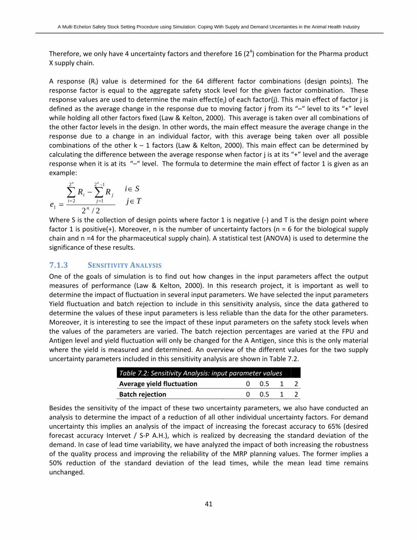
A Multi Echelon Safety Stock Setting Procedure using Simulation: Coping With Supply and Demand Uncertainties in the Animal Health Industry
41
Therefore, we only have 4 uncertainty factors and therefore 16 (24) combination for the Pharma product X supply chain. A response (Ri) value is determined for the 64 different factor combinations (design points). The response factor is equal to the aggregate safety stock level for the given factor combination. These response values are used to determine the main effect(ej) of each factor(j). This main effect of factor j is defined as the average change in the response due to moving factor j from its “–“ level to its “+” level while holding all other factors fixed (Law & Kelton, 2000). This average is taken over all combinations of the other factor levels in the design. In other words, the main effect measure the average change in the response due to a change in an individual factor, with this average being taken over all possible combinations of the other k – 1 factors (Law & Kelton, 2000). This main effect can be determined by calculating the difference between the average response when factor j is at its “+” level and the average response when it is at its “–“ level. The formula to determine the main effect of factor 1 is given as an example:
Where S is the collection of design points where factor 1 is negative (‐) and T is the design point where factor 1 is positive(+). Moreover, n is the number of uncertainty factors (n = 6 for the biological supply chain and n =4 for the pharmaceutical supply chain). A statistical test (ANOVA) is used to determine the significance of these results.
7.1.3 SENSITIVITY ANALYSIS One of the goals of simulation is to find out how changes in the input parameters affect the output measures of performance (Law & Kelton, 2000). In this research project, it is important as well to determine the impact of fluctuation in several input parameters. We have selected the input parameters Yield fluctuation and batch rejection to include in this sensitivity analysis, since the data gathered to determine the values of these input parameters is less reliable than the data for the other parameters. Moreover, it is interesting to see the impact of these input parameters on the safety stock levels when the values of the parameters are varied. The batch rejection percentages are varied at the FPU and Antigen level and yield fluctuation will only be changed for the A Antigen, since this is the only material where the yield is measured and determined. An overview of the different values for the two supply uncertainty parameters included in this sensitivity analysis are shown in Table 7.2.
Table 7.2: Sensitivity Analysis: input parameter values Average yield fluctuation 0 0.5 1 2 Batch rejection 0 0.5 1 2
Besides the sensitivity of the impact of these two uncertainty parameters, we also have conducted an analysis to determine the impact of a reduction of all other individual uncertainty factors. For demand uncertainty this implies an analysis of the impact of increasing the forecast accuracy to 65% (desired forecast accuracy Intervet / S‐P A.H.), which is realized by decreasing the standard deviation of the demand. In case of lead time variability, we have analyzed the impact of both increasing the robustness of the quality process and improving the reliability of the MRP planning values. The former implies a 50% reduction of the standard deviation of the lead times, while the mean lead time remains unchanged.
2/2
2
2
12
11 n
i jji
n n
RRe
∑ ∑=
−
=
−= Tj
Si∈∈
A Multi Echelon Safety Stock Setting Procedure using Simulation: Coping With Supply and Demand Uncertainties in the Animal Health Industry
42
The later has been analyzed by setting the average actual quality lead times at the MRP planning values while keeping the variability equal to the original variability. Moreover, the impact of a reduction of 50% of the quality test repeated has been analyzed.
7.2 RESULTS The results found during the various simulation studies conducted in this research are presented in this section. The heuristic used to determine the results of the simulation model is presented in Appendix XI. The sub questions discussed in section 7.1 are answered for the pharmaceutical supply chain (Pharma product X) in sub section 7.2.1 and for the biological supply chain (Bio product Y) in sub section 7.2.2. The current performance with the actual safety stock levels at Intervet / S‐P A.H. are described prior to the results used to answer the different sub questions. Only the most important Figures are presented in this section, whereas additional Tables and Figures are presented in Appendix XII. The results in this section are given in three different ways, since different stakeholders are interested in different numbers and calculations. These three ways are the inventory in dollars, inventory in logistic months of sales (MoS) and inventory in financial MoS. Inventory in dollars has been calculated by multiplying the total amount of inventory (in kilo grams or vials) by the cost price of these products. The inventory in logistic MoS is calculated by dividing the amount of inventory by the demand per month for these products. The inventory in financial MoS, on the other hand, has been calculated by multiplying the logistic MoS with the relative cost price at each stock point compared to the cost price of the FPP. An overview of the relative cost prices of both Pharma product X and Bio product Y is given in Table 7.3.
Table 7.3: Overview of relative cots prices at pharmaceutical and biological stock points Stock point Avg. Cost Price % of FPP CP Stock point Avg. Cost Price % of FPP CP CONFIDENTIAL
The different types of inventory calculated are the Safety Stock levels, the Quality stock (i.e. WIP, inventory which is not available since it has not been approved by Quality control up to that moment), the Released stock (which is the free available Physical Inventory at the controlled stock points and this is the inventory which can be used for further production or to fulfill demand) and the total inventory (which is the summation of the Physical inventory and the WIP).
7.2.1 PHARMA PRODUCT X The current safety stock settings used at Intervet / S‐P A.H. are given in Appendix VD and these values are used to determine the current performance. The results indicate that a service level of 94% is reached under the current safety stock settings. Intervet / S‐P A.H. expected to reach a service level of approximately 98%, however this model error (i.e. the difference between the expected service level and the realized service level) can be explained by the flexibility which the planners have in real life. The model performance will therefore always be below the actual performance. The 94% is used as a benchmark, since this represents the current performance and will therefore be used as the performance to compare the different scenarios in this research. A graphical presentation of the inventory in dollars is given in Figure 7.1.

A Multi Echelon Safety Stock Setting Procedure using Simulation: Coping With Supply and Demand Uncertainties in the Animal Health Industry
43
Figure 7.1: inventory levels in dollars given the current safety stock settings
Figure 7.1 indicates that in the current situation, the main part of the safety stock is kept at the API stock point. The WIP is mainly located at the FPU and API stock points, which is in line with the expectations, since the main quality test are conducted after the purchasing of API and production of FPU. The WIP levels are approximately equal in the 94% and 98% situation. Sub question 1a,b: The safety stock allocation over the three controlled stock points found resulting in the lowest total inventory costs while reaching the 94% service level and 98% service level are used to answer respectively sub question 1a and 1b. The main results to answer these questions are given in Table 7.4.
Table 7.4: Safety Stock Comparison for the Pharma product X Supply Chain API FPU FPP Total Intervet situation $ 293,424.74 $ 69,125.00 $ 118,460.83 $ 481,010.57 94% situation $ 72,326.73 $ 79,030.00 $ 121,579.74 $ 272,936.47 98% situation $ 103,274.33 $ 92,295.00 $ 295,717.13 $ 491,286.46 Difference Intervet vs 94% $ ‐221,098.01 $ 9,905.00 $ 3,118.91 $‐208,074.10 Difference Intervet vs 98% $ ‐190,150.41 $ 23,170.00 $ 177,256.30 $ 10,275.89 Difference 94% vs 98% $ 30,947.60 $ 13,265.00 $ 174,137.39 $ 218,349.99
Based on the results presented in Table 7.4, one can conclude that a similar performance is reached with a considerable reduction of safety stock costs ($208,074.10) which is a reduction of 43.26%. This reduction is realized by a decline in safety stock at the API stock point and a small safety stock increase at the FPU and FPP stock point. This indicates that safety stock is allocated more downstream in the supply chain (i.e. safety stock shifted more towards the end costumer). This is in line with the expectations, since the main supply uncertainties arise at the FPU level for pharmaceutical supply chains and demand uncertainty affects the FPP level directly. The results also indicate that the model reaches 98% instead of the 94% in the Intervet / S‐P A.H. situation, with a slight increase of total safety stock costs ($10,275.89) and a more downstream allocation of these safety stocks. Moreover, one can conclude that when increasing the model performance from 94% to 98% (actual performance from 98% to approximately 99%), this implies a considerable increase in safety stock costs ($218,349.99, which is an increase of 80%) at mainly the FPP stock point. A graphical comparison of the safety stock distribution is given in Figure 7.2
$ ‐
$ 200.000
$ 400.000
$ 600.000
$ 800.000
$ 1.000.000
API FPU FPP Total
Current Intervet / S‐P A.H. situation
Safety Stock
Average Quality Stock
Average Released Stock
Average Total Inventory

A Multi Echelon Safety Stock Setting Procedure using Simulation: Coping With Supply and Demand Uncertainties in the Animal Health Industry
44
Figure 7.2: Comparison of safety stock distribution over the controlled stock points
A graphical presentation of the average inventory levels at the three controlled stock points in the current situation compared with the 94% and 98% situation is shown in Figure 7.3. Based on the values in Figure 7.3, one can conclude that the total average inventory level achieved by the simulation model is considerably lower than in the current situation (decrease of $236,786.37, which is 27.2%). Moreover, the results indicate that with an average inventory which is approximately equal to the current Intervet / S‐P A.H. inventory in the entire Pharma product X supply chain the performance level reached can be increased from 94% to 98% as a result of a better safety stock allocation over the three controlled stock points.
Figure 7.3: Comparison of average inventory allocation
Sub question 2a,b: The impact on the different stock types of the individual uncertainty factors and the combination of uncertainty factors is determined by using the formula given in sub section 7.1.2. The results gained are given in Figure 7.4. Obviously there is no safety stock necessary when all uncertainty factors are left out of the simulation model and the planning fits the actual situation perfectly. The average quality stock and total inventory in case of no uncertainty are included in the Figures as well.
$293.424,74 ; 61%
$69.125,00 ; 14%
$118.460,83 ; 25%
Intervet / S‐P A.H. situation
API
FPU
FPP
$72.326,73 ; 26%
$79.030,00 ; 29%
$121.579,74 ; 45%
94% situation
API
FPU
FPP
$ ‐
$ 200.000
$ 400.000
$ 600.000
$ 800.000
$ 1.000.000
API FPU FPP TotalIntervet situation $378.128,12 $207.804,12 $284.610,21 $870.542,45
94% situation $166.181,63 $186.407,47 $281.166,97 $633.756,07
98% situation $190.616,71 $226.881,05 $440.387,63 $857.885,39
Total Inven
tory Volum
e
Average Total Inventory Allocation
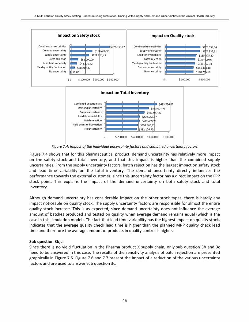
A Multi Echelon Safety Stock Setting Procedure using Simulation: Coping With Supply and Demand Uncertainties in the Animal Health Industry
45
Figure 7.4: Impact of the individual uncertainty factors and combined uncertainty factors
Figure 7.4 shows that for this pharmaceutical product, demand uncertainty has relatively more impact on the safety stock and total inventory, and that this impact is higher than the combined supply uncertainties. From the supply uncertainty factors, batch rejection has the largest impact on safety stock and lead time variability on the total inventory. The demand uncertainty directly influences the performance towards the external customer, since this uncertainty factor has a direct impact on the FPP stock point. This explains the impact of the demand uncertainty on both safety stock and total inventory. Although demand uncertainty has considerable impact on the other stock types, there is hardly any impact noticeable on quality stock. The supply uncertainty factors are responsible for almost the entire quality stock increase. This is as expected, since demand uncertainty does not influence the average amount of batches produced and tested on quality when average demand remains equal (which is the case in this simulation model). The fact that lead time variability has the highest impact on quality stock, indicates that the average quality check lead time is higher than the planned MRP quality check lead time and therefore the average amount of products in quality control is higher. Sub question 3b,c: Since there is no yield fluctuation in the Pharma product X supply chain, only sub question 3b and 3c need to be answered in this case. The results of the sensitivity analysis of batch rejection are presented graphically in Figure 7.5. Figure 7.6 and 7.7 present the impact of a reduction of the various uncertainty factors and are used to answer sub question 3c.
$ 0 $ 100.000 $ 200.000 $ 300.000
No uncertainty
Yield quantity fluctuation
Lead time variability
Batch rejection
Supply uncertainty
Demand uncertainty
Combined uncertainties
$0,00
$28.219,37
$44.376,42
$52.000,09
$127.624,43
$150.456,99
$272.936,47
Impact on Safety stock
$ ‐ $ 100.000 $ 200.000
No uncertainty
Demand uncertainty
Yield quantity fluctuation
Batch rejection
Lead time variability
Supply uncertainty
Combined uncertainties
$140.215,60
$141.140,18
$148.767,31
$149.490,07
$155.375,20
$174.337,61
$175.538,04
Impact on Quality stock
$ ‐ $ 200.000 $ 400.000 $ 600.000 $ 800.000
No uncertainty
Yield quantity fluctuation
Batch rejection
Lead time variability
Supply uncertainty
Demand uncertainty
Combined uncertainties
$382.176,90
$398.365,92
$417.409,75
$424.753,67
$481.047,39
$533.007,73
$633.756,07
Impact on Total Inventory
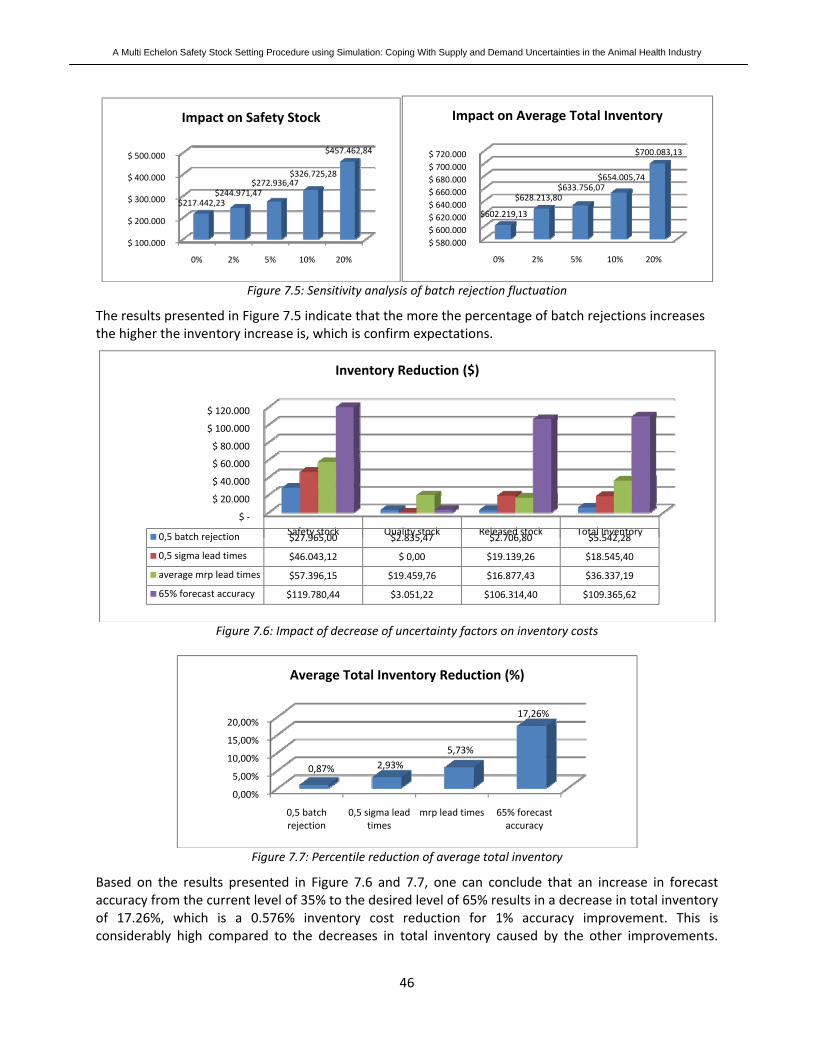
A Multi Echelon Safety Stock Setting Procedure using Simulation: Coping With Supply and Demand Uncertainties in the Animal Health Industry
46
Figure 7.5: Sensitivity analysis of batch rejection fluctuation
The results presented in Figure 7.5 indicate that the more the percentage of batch rejections increases the higher the inventory increase is, which is confirm expectations.
Figure 7.6: Impact of decrease of uncertainty factors on inventory costs
Figure 7.7: Percentile reduction of average total inventory
Based on the results presented in Figure 7.6 and 7.7, one can conclude that an increase in forecast accuracy from the current level of 35% to the desired level of 65% results in a decrease in total inventory of 17.26%, which is a 0.576% inventory cost reduction for 1% accuracy improvement. This is considerably high compared to the decreases in total inventory caused by the other improvements.
$ 100.000
$ 200.000
$ 300.000
$ 400.000
$ 500.000
0% 2% 5% 10% 20%
$217.442,23 $244.971,47
$272.936,47 $326.725,28
$457.462,84
Impact on Safety Stock
$ 580.000 $ 600.000 $ 620.000 $ 640.000 $ 660.000 $ 680.000 $ 700.000 $ 720.000
0% 2% 5% 10% 20%
$602.219,13
$628.213,80 $633.756,07
$654.005,74
$700.083,13
Impact on Average Total Inventory
$ ‐
$ 20.000
$ 40.000
$ 60.000
$ 80.000
$ 100.000
$ 120.000
Safety stock Quality stock Released stock Total Inventory0,5 batch rejection $27.965,00 $2.835,47 $2.706,80 $5.542,28
0,5 sigma lead times $46.043,12 $ 0,00 $19.139,26 $18.545,40
average mrp lead times $57.396,15 $19.459,76 $16.877,43 $36.337,19
65% forecast accuracy $119.780,44 $3.051,22 $106.314,40 $109.365,62
Inventory Reduction ($)
0,00%
5,00%
10,00%
15,00%
20,00%
0,5 batch rejection
0,5 sigma lead times
mrp lead times 65% forecast accuracy
0,87% 2,93%5,73%
17,26%
Average Total Inventory Reduction (%)

A Multi Echelon Safety Stock Setting Procedure using Simulation: Coping With Supply and Demand Uncertainties in the Animal Health Industry
47
Reducing the lead time variability and improving the correctness of the MRP lead times result in a decrease in total inventory as well. This improvement results in a decrease in total inventory of 5.73%. Improving the correctness of the MRP lead times has been tested by adjusting the average lead time of the processes to the MRP lead time for the processes with an average value higher than the MRP lead time. The processes with an average lead time lower than the MRP lead time, remain the same (an overview of the distributions and averages is given in Appendix VF and VIF). These three improvements are of particular interest for the SCM department, since these aspects are to some extent within control of this department. Batch rejection on the other hand is outside the control of the SCM department.
7.2.2 BIO PRODUCT Y The current safety stock settings used at Intervet / S‐P A.H. are given in Appendix VID and these values are used to determine the current performance. The results indicate that a service level of 95% is reached under the current safety stock settings. The 95% service level is from now on used as a benchmark for this supply chain. A graphical presentation of the inventory in dollars is given in Figure 7.8.
Figure 7.8: inventory levels in dollars given the current safety stock settings
Figure 7.8 indicates that in the current situation, the safety stock is, compared to the Pharma product X situation, more equally divided over the three stock points. However, the main part of the safety stock is kept at the most upstream (Antigen) stock point as well. The amount of WIP is considerably higher than in the pharmaceutical supply chain and this is mainly caused by longer average quality control times at the Antigen and FPU stock point. The fact that this quality stock is mainly located at the FPU stock is in compliance with the quality control times at FPU. The WIP levels are again approximately equal in the 95% and 98% situation. Sub question 1a,b: The safety stock allocation over the three controlled stock points found resulting in the lowest total inventory costs while reaching the 95% and 98% service level are used to answer respectively sub question 1a and 1b. The main results to answer these questions are given in Table 7.5.
$ ‐
$ 500.000
$ 1.000.000
$ 1.500.000
$ 2.000.000
$ 2.500.000
$ 3.000.000
$ 3.500.000
$ 4.000.000
$ 4.500.000
$ 5.000.000
Antigen FPU FPP Total
Current Intervet / S‐P A.H. situation
Safety Stock
Average Quality Stock
Average Released Stock
Average Total Inventory
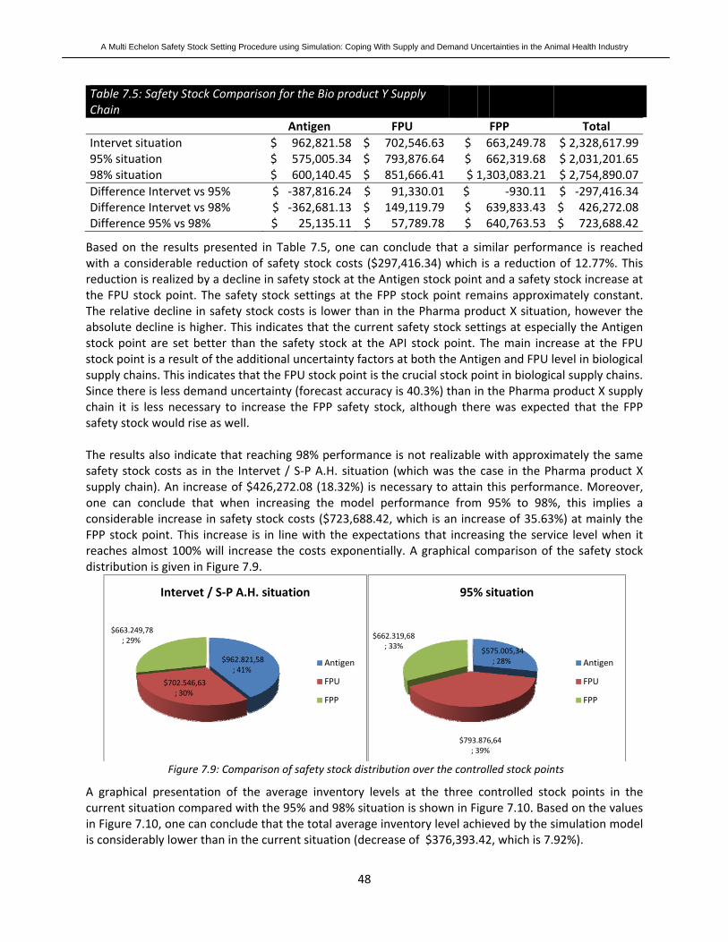
A Multi Echelon Safety Stock Setting Procedure using Simulation: Coping With Supply and Demand Uncertainties in the Animal Health Industry
48
Table 7.5: Safety Stock Comparison for the Bio product Y Supply Chain Antigen FPU FPP Total Intervet situation $ 962,821.58 $ 702,546.63 $ 663,249.78 $ 2,328,617.99 95% situation $ 575,005.34 $ 793,876.64 $ 662,319.68 $ 2,031,201.65 98% situation $ 600,140.45 $ 851,666.41 $ 1,303,083.21 $ 2,754,890.07 Difference Intervet vs 95% $ ‐387,816.24 $ 91,330.01 $ ‐930.11 $ ‐297,416.34 Difference Intervet vs 98% $ ‐362,681.13 $ 149,119.79 $ 639,833.43 $ 426,272.08 Difference 95% vs 98% $ 25,135.11 $ 57,789.78 $ 640,763.53 $ 723,688.42
Based on the results presented in Table 7.5, one can conclude that a similar performance is reached with a considerable reduction of safety stock costs ($297,416.34) which is a reduction of 12.77%. This reduction is realized by a decline in safety stock at the Antigen stock point and a safety stock increase at the FPU stock point. The safety stock settings at the FPP stock point remains approximately constant. The relative decline in safety stock costs is lower than in the Pharma product X situation, however the absolute decline is higher. This indicates that the current safety stock settings at especially the Antigen stock point are set better than the safety stock at the API stock point. The main increase at the FPU stock point is a result of the additional uncertainty factors at both the Antigen and FPU level in biological supply chains. This indicates that the FPU stock point is the crucial stock point in biological supply chains. Since there is less demand uncertainty (forecast accuracy is 40.3%) than in the Pharma product X supply chain it is less necessary to increase the FPP safety stock, although there was expected that the FPP safety stock would rise as well. The results also indicate that reaching 98% performance is not realizable with approximately the same safety stock costs as in the Intervet / S‐P A.H. situation (which was the case in the Pharma product X supply chain). An increase of $426,272.08 (18.32%) is necessary to attain this performance. Moreover, one can conclude that when increasing the model performance from 95% to 98%, this implies a considerable increase in safety stock costs ($723,688.42, which is an increase of 35.63%) at mainly the FPP stock point. This increase is in line with the expectations that increasing the service level when it reaches almost 100% will increase the costs exponentially. A graphical comparison of the safety stock distribution is given in Figure 7.9.
Figure 7.9: Comparison of safety stock distribution over the controlled stock points
A graphical presentation of the average inventory levels at the three controlled stock points in the current situation compared with the 95% and 98% situation is shown in Figure 7.10. Based on the values in Figure 7.10, one can conclude that the total average inventory level achieved by the simulation model is considerably lower than in the current situation (decrease of $376,393.42, which is 7.92%).
$962.821,58 ; 41%
$702.546,63 ; 30%
$663.249,78 ; 29%
Intervet / S‐P A.H. situation
Antigen
FPU
FPP
$575.005,34 ; 28%
$793.876,64 ; 39%
$662.319,68 ; 33%
95% situation
Antigen
FPU
FPP

A Multi Echelon Safety Stock Setting Procedure using Simulation: Coping With Supply and Demand Uncertainties in the Animal Health Industry
49
In contrast with the Pharma product X supply chain, there is a considerable difference between the average inventory in the entire Bio product Y supply chain in the current Intervet / S‐P A.H. situation and the 98% situation. A better safety stock allocation does therefore not result in an increase in performance from 95% to 98% with equal average total inventory.
Figure 7.10: Comparison of average inventory allocation
Sub question 2a,b: The impact on the different stock types of the individual uncertainty factors and the combination of uncertainty factors is determined by using the formula given in sub section 7.1.2. The results gained are given in Figure 7.11.
Figure 7.11: Impact of the individual uncertainty factors and combined uncertainty factors
$ ‐
$ 1.000.000
$ 2.000.000
$ 3.000.000
$ 4.000.000
$ 5.000.000
Antigen FPU FPP TotalIntervet situation $1.438.999,57 $1.939.562,22 $1.376.556,73 $4.755.118,52
95% situation $1.070.344,40 $1.978.646,49 $1.329.734,21 $4.378.725,10
98% situation $1.089.281,99 $2.080.660,71 $2.000.485,54 $4.987.246,43
Total Inven
tory Volum
eAverage Total Inventory Allocation
$ ‐ $ 1.000.000 $ 2.000.000
No uncertainty
Test repetition
Batch rejection
Demand uncertainty
Combined uncertainties
$‐
$399.882,82
$494.694,42
$506.885,78
$653.364,60
$975.041,47
$1.144.207,80
$1.443.740,73
$2.031.201,65
Impact on Safety stock
$ ‐ $ 1.000.000 $ 2.000.000
No uncertainty
Yield quantity fluctuation
Yield activity fluctuation
Lead time variability
Combined uncertainties
$1.271.133,62
$1.361.933,87
$1.392.987,14
$1.402.293,22
$1.405.491,78
$1.419.162,42
$1.763.298,90
$1.828.046,40
$1.845.447,31
Impact on Quality stock
$ ‐ $ 1.000.000 $ 2.000.000 $ 3.000.000 $ 4.000.000 $ 5.000.000
No uncertainty
Yield quantity fluctuation
Batch rejection
Lead time variability
Combined uncertainties
$2.605.894,34 $2.966.841,30 $3.058.540,59 $3.083.176,53 $3.137.704,11 $3.326.993,50 $3.503.917,05
$3.887.240,49 $4.378.725,10
Impact on Total Inventory

A Multi Echelon Safety Stock Setting Procedure using Simulation: Coping With Supply and Demand Uncertainties in the Animal Health Industry
50
Figure 7.11 shows that for the biological supply chain, in contradiction of the pharmaceutical supply chain, the supply uncertainty has the main impact on the safety stock and total inventory. This contradiction is a result of the increased amount of supply uncertainty in the biological supply chains (i.e. additional uncertainty factors test repetition and yield activity fluctuation). This is in line with the expectation that there are more supply uncertainty factors in biological supply chains compared to the pharmaceutical supply chains. Although, demand uncertainty still has the main impact on the amount of safety stock, when comparing the individual uncertainty factors, the impact of the individual supply uncertainty factors (lead time variability in particular) is relatively higher in this biological supply chain when comparing the impact values with the pharmaceutical supply chain. This is a result of batch rejections on both the Antigen and FPU level (instead of only the FPU level in the pharmaceutical supply chain) and longer and more variable average quality control lead times in the biological supply chains. In line with the expectations, the supply uncertainty factors are again responsible for almost the entire quality stock increase. The fact that lead time variability has the highest impact on quality stock, indicates that the average quality check lead time is higher than the planned MRP quality check lead time and therefore the average amount of products in quality control is higher. Sub question 3a,b and c: For this biological supply chain all sub question need to be answered. The results of the sensitivity analysis of batch rejection are presented in Figure 7.12 and 7.13. Figure 7.14 and 7.15 present the impact of a reduction of the various uncertainty factors and are used to answer sub question 3c.
Figure 7.12: Sensitivity analysis of yield activity fluctuation
Figure 7.13: Sensitivity analysis of batch rejection
$ 1.700.000 $ 1.800.000 $ 1.900.000 $ 2.000.000 $ 2.100.000 $ 2.200.000 $ 2.300.000
0 * normal 0,5* normal
normal fluctuation
2 * normal
$1.898.797,76 $1.947.055,96
$2.031.201,65
$2.251.952,04
Impact on Safety stock
$ 4.000.000 $ 4.100.000 $ 4.200.000 $ 4.300.000 $ 4.400.000 $ 4.500.000 $ 4.600.000
0 * normal 0,5* normal
normal fluctuation
2 * normal
$4.202.892,32 $4.238.873,60
$4.378.725,10
$4.577.224,52
Impact on Average Total Inventory
$ 1.700.000
$ 1.800.000
$ 1.900.000
$ 2.000.000
$ 2.100.000
$ 2.200.000
$ 2.300.000
0 * normal 0,5 * normal
normal rejection
2 * normal
$1.767.653,28
$1.916.713,91
$2.031.201,65
$2.306.347,03
Impact on Safety stock
$ 4.000.000
$ 4.100.000
$ 4.200.000
$ 4.300.000
$ 4.400.000
$ 4.500.000
$ 4.600.000
0 * normal 0,5 * normal
normal rejection
2 * normal
$4.123.751,82
$4.235.635,77
$4.378.725,10
$4.602.107,54
Impact on Average Total Inventory
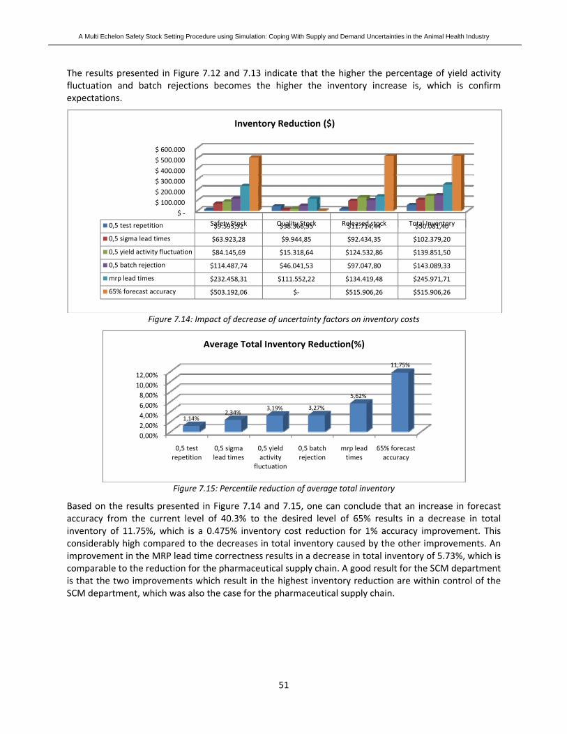
A Multi Echelon Safety Stock Setting Procedure using Simulation: Coping With Supply and Demand Uncertainties in the Animal Health Industry
51
The results presented in Figure 7.12 and 7.13 indicate that the higher the percentage of yield activity fluctuation and batch rejections becomes the higher the inventory increase is, which is confirm expectations.
Figure 7.14: Impact of decrease of uncertainty factors on inventory costs
Figure 7.15: Percentile reduction of average total inventory
Based on the results presented in Figure 7.14 and 7.15, one can conclude that an increase in forecast accuracy from the current level of 40.3% to the desired level of 65% results in a decrease in total inventory of 11.75%, which is a 0.475% inventory cost reduction for 1% accuracy improvement. This considerably high compared to the decreases in total inventory caused by the other improvements. An improvement in the MRP lead time correctness results in a decrease in total inventory of 5.73%, which is comparable to the reduction for the pharmaceutical supply chain. A good result for the SCM department is that the two improvements which result in the highest inventory reduction are within control of the SCM department, which was also the case for the pharmaceutical supply chain.
$ ‐$ 100.000
$ 200.000 $ 300.000 $ 400.000
$ 500.000 $ 600.000
Safety Stock Quality Stock Released stock Total Inventory0,5 test repetition $9.595,92 $38.366,95 $11.714,44 $50.081,40
0,5 sigma lead times $63.923,28 $9.944,85 $92.434,35 $102.379,20
0,5 yield activity fluctuation $84.145,69 $15.318,64 $124.532,86 $139.851,50
0,5 batch rejection $114.487,74 $46.041,53 $97.047,80 $143.089,33
mrp lead times $232.458,31 $111.552,22 $134.419,48 $245.971,71
65% forecast accuracy $503.192,06 $‐ $515.906,26 $515.906,26
Inventory Reduction ($)
0,00%2,00%4,00%6,00%8,00%10,00%12,00%
0,5 test repetition
0,5 sigma lead times
0,5 yield activity
fluctuation
0,5 batch rejection
mrp lead times
65% forecast accuracy
1,14%2,34%
3,19% 3,27%
5,62%
11,75%
Average Total Inventory Reduction(%)

A Multi Echelon Safety Stock Setting Procedure using Simulation: Coping With Supply and Demand Uncertainties in the Animal Health Industry
52
8 CONCLUSIONS AND RECOMMENDATIONS (IMPLEMENTATION) This final chapter presents the overall conclusions of this research project based on the results discussed in the previous chapters in section 8.1. Hereafter, the discussion section including managerial implications, research implications, future research and limitations are discussed in section 8.2.
8.1 CONCLUSIONS The initial problem definition for this research project was formulated as follows:
Provide quantitative insight in which inventory management methods / approaches should be taken into account to reach an external service level against minimal inventory costs
An inventory management framework has been developed, which distinguishes three different inventory types (i.e. work in process, cycle stock and safety stock) and associated optimization methods. From this framework, the optimization method which was most directly related to the service level and uncertainties in the supply chain was selected and this resulted in a quantitative model, the multi echelon safety stock simulation model developed during this research project. Moreover a clear service level definition and measure have been formulated. After having selected the best applicable optimization method, the final research question which needed to be answered during this research project was formulated:
What is the impact of the different uncertainty factors on the safety stock levels and what is the optimal safety stock level at the various stock points to reach the service level against minimal inventory costs?
The simulation study shows that the results of the safety stock model result in a considerable decrease in the safety stock and average total inventory compared to the current situation, mainly realized by an safety stock shift from the upstream API/Antigen stock points to the more downstream FPU and FPP stock points. This indicates that the multi‐echelon model outperforms the current single echelon models and rules in the Intervet /S‐P A.H. supply chain. Furthermore, the results indicate that further increasing the service level to almost one hundred percent results in an extreme increase in inventory costs primarily at the FPP stock point and this cost increase is many times higher than the Backlog cost reduction realized by this performance improvement. A comparison of the results indicates that demand uncertainty has relatively more impact on the safety stock and average total inventory for the pharmaceutical supply chain and the combined supply uncertainties, lead time variability in particular, for the biological supply chain. This is a result of the increased number of supply uncertainties in the biological supply chains. The results also show that Work In Process is almost only affect by supply uncertainty and especially lead time variability. Moreover, the results show that improving forecast accuracy and increasing MRP lead time correctness result in the largest inventory cost reduction and that reducing the number of test repetitions result in the smallest inventory cost reduction. Therefore, the conclusion of this research project is that the research question has been answered and that the quantitative insights gained by the results of the safety stock model are an ideal starting point for future improvement programs and future research, since the main influencing uncertainty factors are within control of the SCM department, where this research project has been initiated.

A Multi Echelon Safety Stock Setting Procedure using Simulation: Coping With Supply and Demand Uncertainties in the Animal Health Industry
53
8.2 DISCUSSION In this section three separate aspects are discussed. The managerial implications and recommendations are presented in sub section 8.2.1. Hereafter, the scientific implications of this research project is described in sub section 8.2.2. Finally, future research based on this research project and the limitations of this research project are discussed in sub section 8.2.3.
8.2.1 MANAGERIAL IMPLICATIONS AND RECOMMENDATIONS This study results in several implications for the pharmaceutical business and for Intervet / S‐P A.H. in particular. First of all, we have concluded that moving the safety stock more downstream and reducing the amount of safety stock at the most upstream stock point results in reaching the same service level with lower total inventory costs. Moreover, a clear investigation has been made to distinguish the impact of the different uncertainty factors on the total inventory in the pharmaceutical and biological supply chains. This can help organizations to priorities their future improvement programs and research. Furthermore, a clear service level definition has been formulated and this service level can be calculated and used throughout the organization. The most important recommendation is to make use of the outcomes of the safety stock model in future improvement programs. This research clearly identifies the improvement possibilities on inventory management and can be ideally used for prioritization. Moreover, using this model will result in a reduction of the total inventory costs. However, the model cannot be used for seasonal products, since a stationary demand is assumed. The second recommendation is to shift the safety stock more downstream towards the end customer. The simulation model can be used to determine the allocation over the controlled stock points. The third recommendation is to clearly distinguish the different types of inventory through the organization. Different types of inventory are used for different reasons and different organization levels are responsible for these inventory types. Therefore, it is of considerable importance to be able to identify and trace the different inventory types in the supply chain. The fourth recommendation is to make use of the service level definition provided in this research. This service level measure resembles the performance of the Intervet / S‐P A.H. performance properly and is best applicable when optimizing the total margin volume in dollars.
8.2.2 SCIENTIFIC IMPLICATIONS Considerable attention has been paid to the demand uncertainty factor in safety stock models, however relatively less research incorporated the various supply uncertainty factors (e.g. lead time uncertainty, yield uncertainty, batch rejection) in a multi echelon supply chain. Within this research project a simulation model has been developed to determine the optimal safety stock allocation over the controlled stock points in a multi echelon supply chain, coping with both supply and demand uncertainty. Moreover, this quantitative model has been implemented in a software application. This is definitely a contribution to the current scientific field of operations research. Furthermore, the quantitative analysis of the impact of the various uncertainty factors in the pharmaceutical industry has not been conducted in this setting. Although this research was only conducted in the pharmaceutical industry and only for two products, the results indicate that in general the impact of demand uncertainty is higher than an individual supply uncertainty factor. However, especially for biological supply chains, the combined supply uncertainty factors do have a relatively large impact as well.
A Multi Echelon Safety Stock Setting Procedure using Simulation: Coping With Supply and Demand Uncertainties in the Animal Health Industry
54
Moreover, the comparison of different uncertainty reduction methods, which indicates that increasing the forecast accuracy results in the largest inventory cost reduction compared to other uncertainty reduction methods, is a contribution to the current literature. Furthermore, an inventory management framework which gives an overview of different optimization methods for three types of inventory is given. Therefore this research contributes both to the research on inventory management as well as to the research in the pharmaceutical and biological industry.
8.2.3 LIMITATIONS AND FUTURE RESEARCH Despite the contributions of this study to the inventory management literature and pharmaceutical and biological industry, it is subject to some limitations. Among the limitations of this study is the fact that the simulation model used is not generalizable and should therefore be adapted for different supply chain structures. This makes the model harder to implement in the current business setting. However, although it takes some time, it is definitely worth the effort. Another limitation of this research, is that production capacity and product shelf life were beyond the scope of this research and thus not taken into account in the simulation model. However, order quantities are taken as constant as well and these quantities are set with shelf life taken into account. Therefore, not taken into account shelf life, does not affect the results of this research. Finally, the demand patterns of the products used are relatively constant and there is no trend or seasonal pattern. Therefore, the simulation model cannot be used for seasonal products. There are a number potentially interesting directions for future research. Firstly, the impact of the capacity on the service level needs further attention. Capacity might be restricting and therefore affect the performance at the various stock points. This study also revealed that reducing the lead time variability or reducing the (quality control) lead times would result in a decline in total inventory costs. A tradeoff between an increase in capacity to reduce the lead times and thus reduce the total inventory costs would be an interesting research in this particular industry. This implies a research on reducing Work In Process, which is a major part of the inventory in especially the biological supply chains and is therefore of considerable interest for this industry and for the inventory management field as well. Furthermore, there are several possibilities for future research which can be based on the results of this research project. This includes an investigation of how to improve the forecast accuracy in the current organization. Since the results of this research indicate that a reduction in demand uncertainty results in the largest cost reduction, this is definitely an interesting topic for future research for Intervet / S‐P A.H. Moreover, quantitatively investigating the benefits of changing the current MRP planning system into a more advanced planning system would be interesting for Intervet / S‐P A.H, as well as investigating the impact of better capacity planning at the manufacturing site. These future research topics are particularly interesting in combination with the current VMI rollout. Hopefully, next to understanding the pharmaceutical industry and the complex supply chains, with the various uncertainty factors in particular, this study will also trigger scholars to further investigate the inventory management optimization possibilities in this challenging and interesting industry. Since this research project is one in a row of a series of consecutive research projects conducted at Intervet / S‐P A.H., this master thesis can be used as a solid starting point for future research.

A Multi Echelon Safety Stock Setting Procedure using Simulation: Coping With Supply and Demand Uncertainties in the Animal Health Industry
55
REFERENCES - Bertrand, J.W.M. & Fransoo, J. C. (2002). Modelling and Simulation: Operations management
research methodologies using quantitative modelling. International Journal of Operations and Production Management, 22(2), 241‐264.
- Bollapragada, R., Roa, U.S. & Zhang, J. (2004). Managing two‐stage serial inventory systems under demand and supply uncertainty and customer service level requirements. IIE Transactions, 36, 73‐85.
- Burgin, T.A. (1975). The Gamma Distribution and Inventory Control. Operational Research Quarterly, 26(3), 507‐525.
- De Kok, A.G. & Graves, S. (2003). Supply Chain Management: Design, Coordination and Operation. Amsterdam: Elsevier, Chapter 1.
- Hopp, W.J. & Spearman, M.L. (1996). Factory Physics. Boston, MA: Irwin/McGraw Hill. - Kelle, P. & Silver, E.A. (2006). Safety stock reduction by order splitting. Naval Research Logistics, 37,
725‐743.
- Kleijnen, J.P.C. (1995), Verification and validation of simulation models; Theory and Methodology. European Journal of Operational Research, 82, 145‐162.
- Law, A.M. & Kelton, W.D. (2000). Simulation Modelling and Analysis (3rd ed.). New York, NY: McGraw‐Hill.
- Minner, S. (2001). Strategic safety stocks in reverse logistics supply chains. International Journal of Production Economic, 71, 417‐428.
- Mitroff, I., Betz, F., Pondy, L. & Sagasti, F. (1974). On managing science in the systems age: two schemas for the study of science as a whole systems phenomenon. Interfaces, 4(3), 46‐58.
- Mohebbi, E. (2004). A replenishment model for the supply‐uncertainty problem. International Journal of Production Economics, 87, 25‐37.
- Nahmias, S. (2005). Production and Operations Analysis (5th ed.). New York, NY: McGraw‐Hill. - Schering Plough (2008). Financial report. Retrieved April 23, 2009.
- Shah, N. (2004). Pharmaceutical supply chains: key issues and strategies for optimization. Computers and Chemical Engineering, 28, 929‐941.
- Silver, E.A., Pyke, D.F. & Peterson, R. (1998). Inventory Management and Production Planning and Scheduling (3rd ed.). New York, NY: Wiley.
- Spitter, J. (2005). Rolling Schedule Approaches for Supply Chain Operations Planning. PhD thesis, Eindhoven University of Technology, the Netherlands.
- Talluri, S., Cetin, K. & Gardner, A.J. (2004). Integrating demand and supply variability into safety stock evaluations. International Journal of Physical Distribution & Logistics Management, 34(1), 62‐69.
- Teulings, M.F. & van der Vlist, P. (2001). Managing the supply chain with standard mixed loads. International Journal of Physical Distribution & Logistics Management, 3, 169‐186.

A Multi Echelon Safety Stock Setting Procedure using Simulation: Coping With Supply and Demand Uncertainties in the Animal Health Industry
56
- Teunter, R.H. & Flapper, S.D.P. (2006). A comparison of bottling alternatives in the pharmaceutical industry. Journal of Operations Management, 24, 215‐234.
- Thomas, D.J. & Tyworth, J.E. (2006). Pooling lead‐time risk by order splitting: A critical review. Transportation Research Part E, 42, 245‐257.
- Walkenhorst, J.S. (2007). Quantifying the Value of Reduced Lead Time and Increased Delivery Frequency. MSc Thesis, Massachusetts Institute of Technology, United States.

A Multi Echelon Safety Stock Setting Procedure using Simulation: Coping With Supply and Demand Uncertainties in the Animal Health Industry
57
APPENDICES
APPENDIX I: GEOGRAPHICAL LOCATION OF SITES CONFIDENTIAL

A Multi Echelon Safety Stock Setting Procedure using Simulation: Coping With Supply and Demand Uncertainties in the Animal Health Industry
58
APPENDIX II: SKUS PER COUNTRY CONFIDENTIAL
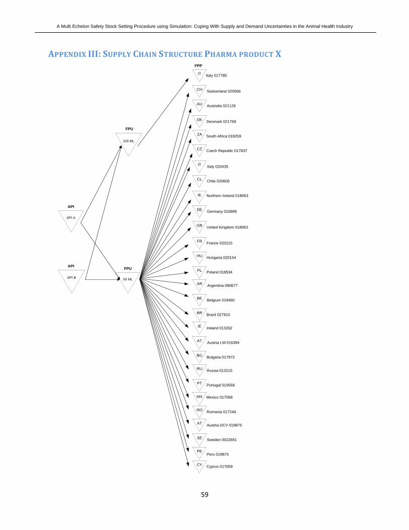
A Multi Echelon Safety Stock Setting Procedure using Simulation: Coping With Supply and Demand Uncertainties in the Animal Health Industry
59
APPENDIX III: SUPPLY CHAIN STRUCTURE PHARMA PRODUCT X
API A
IT
100 ML
API B 50 ML
CY
PE
SE
AT
RO
MX
PT
RU
BG
AT
IE
BR
BE
AR
PL
HU
FR
GB
DE
IE
CL
IT
CZ
ZA
DK
AU
CH
Italy 017785
Switzerland 020566
Argentina 090677
Poland 018534
Hungaria 020154
France 020215
United Kingdom 018063
Germany 020899
Northern Ireland 018063
Chile 020605
Italy 020435
Czech Republic 017837
South Africa 019259
Denmark 021759
Australia 021126
Cyprus 017659
Peru 019875
Sweden 0022651
Austria DCV 019875
Romania 017244
Mexico 017068
Portugal 019566
Russia 013215
Bulgaria 017972
Austria LM 016394
Ireland 013262
Brazil 027915
Belgium 019460
FPU
FPU
API
API
FPP

A Multi Echelon Safety Stock Setting Procedure using Simulation: Coping With Supply and Demand Uncertainties in the Animal Health Industry
60
APPENDIX IV: SUPPLY CHAIN STRUCTURE BIO PRODUCT Y

A Multi Echelon Safety Stock Setting Procedure using Simulation: Coping With Supply and Demand Uncertainties in the Animal Health Industry
61
APPENDIX V: INPUT PARAMETERS PHARMA PRODUCT X A. GENERAL INPUT: BOM FACTORS PHARMA PRODUCT X BOM Factors Bio Product Y Component Component Qty Material Material Qty API 001151 1 kg API 001148 1 kg API 001148 0.275 kg Bulk Pharma product X 100 kg API 030767 0.131 kg Bulk Pharma product X 100 kg Bulk Pharma product X 10.28 kg Pharma product X FPU 100 ML 100 vials 5.14 kg Pharma product X FPU 50 ML 100 vials Pharma product X FPU 100 ML 100 vials Pharma product X FPP 100 ML 100 vials Pharma product X FPU 50 ML 100 vials Pharma product X FPP 50 ML 100 vials Fixed Quantities Bio Product Y A Fixed Quantity A 20 ML 3000GR (Gram) Fixed Quantity A 50 ML 4500GR (Gram) Fixed Quantity A 100 ML 6000GR (Gram) Bio product Y Fixed Quantity Bio product Y50 ML 4500GR (Gram) Fixed Quantity Bio product Y 20 ML 3000GR (Gram) B Fixed Quantity B 50 ML 4500GR (Gram) Fixed Quantity B 20 ML 3000GR (Gram) Fixed Quantities Pharma product X Pharma product X Fixed Quantity Pharma product X 50 ML 3000GR (Gram) Fixed Quantity Pharma product X 100 ML 5000GR (Gram)

A Multi Echelon Safety Stock Setting Procedure using Simulation: Coping With Supply and Demand Uncertainties in the Animal Health Industry
62
B. GENERAL INPUT: COST PARAMETERS PHARMA PRODUCT X CONFIDENTIAL

A Multi Echelon Safety Stock Setting Procedure using Simulation: Coping With Supply and Demand Uncertainties in the Animal Health Industry
63
C. GENERAL INPUT: MRP LEAD TIMES PHARMA PRODUCT X ComOp UIN MRP PT MRP QT MRP TT MRP PLT MRP PTF
1 IT ‐ Italy ‐ Intervet Italia 017785 2 3 5 10 352 CH ‐ Switzerland 020566 2 3 2 10 353 AU ‐ Australia 021126 2 3 5 10 354 DK ‐ Denmark 021759 2 3 2 10 355 ZA ‐ South Africa 019259 2 15 5 10 356 CZ ‐ Czech Republic 017837 2 3 5 10 357 IT ‐ Italy ‐ Intervet Italia 020435 2 3 5 10 358 CL ‐ Chile 020605 2 3 5 10 359 IE ‐ Northern Ireland 018063 2 3 2 10 35
10 DE ‐ Germany 020899 2 3 2 10 3511 GB ‐ United Kingdom 018063 2 8 2 10 3512 FR ‐ France 020215 2 3 2 10 3513 HU ‐ Hungaria 020154 2 3 5 10 3514 PL ‐ Poland 018534 2 3 5 10 3515 AR ‐ Argentina 090667 2 30 5 10 3516 BE ‐ Belgium 019460 2 3 2 10 3517 BR ‐ Brazil 027915 2 30 5 10 3518 IE ‐ Ireland 013262 2 3 2 10 3519 AT ‐ Austria ‐ LM 016394 2 3 5 10 3520 BG ‐ Bulgaria 017972 2 3 5 10 3521 RU ‐ Russia 013215 2 3 7 10 3522 PT ‐ Portugal 019566 2 3 5 10 3523 MX ‐ Mexico 017068 2 3 5 10 3524 RO ‐ Romania 017244 2 3 6 10 3525 AT ‐ Austria ‐ DCV 019875 2 3 5 10 3526 SE ‐ Sweden 022651 2 3 2 10 3527 PE ‐ Peru 019875 2 3 5 10 3528 CY ‐ Cyprus 017659 2 3 6 10 3535 FPU 100 ML 004156 3 48 0 0 14036 FPU 50 ML 004157 3 48 0 0 14037 Bulk 002135 3 10 0 0 3538 API 1 030767 0 42 90 0 039 API 2 001148 0 55 14 0 040 API 3 001151 0 42 90 0 0

A Multi Echelon Safety Stock Setting Procedure using Simulation: Coping With Supply and Demand Uncertainties in the Animal Health Industry
64
D. GENERAL AND DEMAND UNCERTAINTY PARAMETERS PHARMA PRODUCT X ComOp UIN Demand/w Sigma Beta Alpha Q Safety Stock 1 IT ‐ Italy ‐ Intervet Italia 017785 265.15 141.10 75.08 3.53 3400 662 2 CH ‐ Switzerland 020566 24.50 17.19 12.06 2.03 560 45 3 AU ‐ Australia 021126 91.90 87.98 84.23 1.09 1360 239 4 DK ‐ Denmark 021759 135.00 197.42 288.70 0.47 384 23 5 ZA ‐ South Africa 019259 99.75 82.22 67.78 1.47 1680 700 6 CZ ‐ Czech Republic 017837 69.73 175.73 442.87 0.16 1200 218 7 IT ‐ Italy ‐ Intervet Italia 020435 103.44 242.37 567.89 0.18 1920 434 8 CL ‐ Chile 020605 45.19 65.85 95.95 0.47 1280 105 9 IE ‐ Northern Ireland 018063 16.58 19.41 22.73 0.73 560 25 10 DE ‐ Germany 020899 120.69 310.71 799.94 0.15 2000 422 11 GB ‐ United Kingdom 018063 148.92 577.41 2238.87 0.07 2720 683 12 FR ‐ France 020215 449.35 663.91 980.91 0.46 4000 2400 13 HU ‐ Hungaria 020154 202.17 452.26 1011.70 0.20 3120 1442 14 PL ‐ Poland 018534 436.27 875.54 1757.08 0.25 4480 3000 15 AR ‐ Argentina 090667 147.23 197.06 263.75 0.56 3440 428 16 BE ‐ Belgium 019460 122.35 197.23 317.92 0.38 2000 362 17 BR ‐ Brazil 027915 499.46 1350.97 3654.18 0.14 6000 6000 18 IE ‐ Ireland 013262 16.58 19.41 22.73 0.73 720 34 19 AT ‐ Austria ‐ LM 016394 40.23 43.85 47.79 0.84 1200 100 20 BG ‐ Bulgaria 017972 33.77 20.54 12.49 2.70 1120 90 21 RU ‐ Russia 013215 665.63 1239.77 2309.14 0.29 7280 9200 22 PT ‐ Portugal 019566 286.17 596.44 1243.13 0.23 4320 1167 23 MX ‐ Mexico 017068 72.85 74.26 75.69 0.96 960 100 24 RO ‐ Romania 017244 80.25 179.68 402.33 0.20 2880 600 25 AT ‐ Austria ‐ DCV 019875 147.48 446.93 1354.38 0.11 2880 594 26 SE ‐ Sweden 022651 11.50 7.34847 4.70 2.45 576 24 27 PE ‐ Peru 019875 9.88 21.24 45.69 0.22 400 30 28 CY ‐ Cyprus 017659 25.50 105.96 440.29 0.06 3072 256 35 FPU 100 ML 004156 265.15 3400 500 36 FPU 50 ML 004157 4102.36 24250 20000 37 Bulk 002135 238.12 1260 0 38 API 1 030767 0.31 14 4 39 API 2 001148 0.65 9 35 40 API 3 001151 0.65 9 0

A Multi Echelon Safety Stock Setting Procedure using Simulation: Coping With Supply and Demand Uncertainties in the Animal Health Industry
65
E. SUPPLY UNCERTAINTY PARAMETERS PHARMA PRODUCT X Batch Rejections Pharma product X APIs # of batches Percentage rejected 0 0.00% accepted 80 100.00% total 80 100.00% Bulk # of batches Percentage rejected 1 2.94% accepted 33 97.06% Total 34 100.00% FPU # of batches Percentage rejected 4 7.55% accepted 49 92.45% Total 53 100.00% FPP # of batches Percentage rejected 0 0.00% accepted 389 100.00% Total 389 100.00% Batch value deviation Pharma product X Bulk ‐0.17% FPU 50 ML 1.11% FPU 100 ML ‐3.98% FPP ‐0.08%

A Multi Echelon Safety Stock Setting Procedure using Simulation: Coping With Supply and Demand Uncertainties in the Animal Health Industry
66
F. SUPPLY UNCERTAINTY PARAMETERS: STOCHASTIC LEAD TIMES PHARMA PRODUCT X API Lead Time Characteristics API 001151 MRP PTF MRP Target Average Distribution Quality Time 42 27 Gamma(10.438;2.5867) Transportation Time 90 120.59 Weibull(1.7731;135.5) Total Time 132 147.59 API 001148 MRP PTF MRP Target Average Distribution Quality Time 55 42.5834 Gamma(61.249;0.69525) Transportation Time 14 17.27 Gamma(7.359;2.3467) Total Time 69 59.85 API 030767 MRP PTF MRP Target Average Distribution Quality Time 42 43.36 Triang(0;26;104.08) Transportation Time 90 104.71 Weibull(1.6602;117.15) Total Time 132 148.07 Bulk Lead Time Characteristics Pharma product X Bulk MRP PTF MRP Target Average Distribution Quality Time 35 10 29.96 Expo(29.963) Planning Time 0 47.52 Triang(0;48;94.548) Process Time 3 1.68 Emperical Total Time 35 79.16 FPU Lead Time Characteristics Pharma product X FPU 100 ML MRP PTF MRP Target Average Distribution Quality Time 140 48 58.85 Logn(58.847;23.257) Planning Time 0 61.52 Weibull(2.6838;69.197) Process Time 3 1.54 Emperical Total Time 140 121.91 Pharma product X FPU 50 ML MRP PTF MRP Target Average Distribution Quality Time 140 48 58.847 Logn(58.847;23.257) Planning Time 0 61.52 Weibull(2.6838;69.197) Process Time 3 1.542 Emperical Total Time 140 121.92 FPP Lead Time Characteristics FPP 100 ML MRP PTF MRP Target Average Distribution Quality Time MRP value MRP value Expo(2.0513) Process Time 10 11.23 Emperical Transportation Time MRP value MRP value Deterministic FPP 50 ML MRP PTF MRP Target Average Distribution Quality Time MRP value MRP value Expo(2.0513) Process Time 10 11.23 Emperical

A Multi Echelon Safety Stock Setting Procedure using Simulation: Coping With Supply and Demand Uncertainties in the Animal Health Industry
67
Transportation Time MRP value MRP value Deterministic
APPENDIX VI: INPUT PARAMETERS BIO PRODUCT Y A. GENERAL INPUT: BOM FACTORS BIO PRODUCT Y BOM Factors Bio product Y Component Component Qty Material Material Qty Antigen A NL10 10 kg Bulk A NL10 100 kg 20 kg Bulk Bio product Y 100 kg Antigen B GB10 10 kg Antigen A ES10 10 kg Antigen A ES10 10 kg Bulk A ES10 100 kg Antigen B NL10 18.2 kg Bulk B 100 kg 18.2 kg Bulk Bio product Y 100 kg Bulk A NL10 2.2 kg FPU A 20 ML 100 vials 5.271 kg FPU A 50 ML 100 vials 10.476 kg FPU A 100 ML 100 vials Bulk A ES10 27.397 kg FPU A 250 ML P 100 vials 27.397 kg FPU A 250 ML T 100 vials
Bulk Bio product Y 5.3 kg FPU Bio product Y 20 ML 100 vials
2.2 kg FPU Bio product Y 50 ML 100 vials
Bulk B 5.327 kg FPU B 20 ML 100 vials 2.231 kg FPU B 50 ML 100 vials FPU A 20 ML 100 vials FPP A 20 ML 100 vials FPU A 50 ML 100 vials FPP A 50 ML 100 vials FPU A 100 ML 100 vials FPP A 100 ML 100 vials FPU A 250 ML P 100 vials FPP A 250 ML P 100 vials FPU A 250 ML T 100 vials FPP A 250 ML T 100 vials FPU Bio product Y 20 ML 100 vials
FPP Bio product Y 20 ML 100 vials
FPU Bio product Y 50 ML 100 vials
FPP Bio product Y 50 ML 100 vials
FPU B 20 ML 100 vials FPP B 20 ML 100 vials FPU B 50 ML 100 vials FPP B 50 ML 100 vials

A Multi Echelon Safety Stock Setting Procedure using Simulation: Coping With Supply and Demand Uncertainties in the Animal Health Industry
68
B. GENERAL INPUT: COST PARAMETERS BIO PRODUCT Y
CONFIDENTIAL

A Multi Echelon Safety Stock Setting Procedure using Simulation: Coping With Supply and Demand Uncertainties in the Animal Health Industry
69
C. GENERAL INPUT: MRP LEAD TIMES BIO PRODUCT Y ComOp UIN MRP PT MRP QT MRP TT MRP PLT MRP PTF 1 CH ‐ Switzerland 013610 2 3 2 10 35 2 SE ‐ Sweden 035629 2 3 2 10 35 3 CH ‐ Switzerland 013582 2 3 2 10 35 4 DK ‐ Denmark 013592 2 3 2 10 35 5 FI ‐ Finland 013913 2 3 5 10 35 6 IT ‐ Italy ‐ Intervet Italia 013314 2 3 5 10 35 7 BE ‐ Belgium 013308 2 30 2 10 35 8 GR ‐ Greece 013313 2 3 5 10 35 9 AT ‐ Austria ‐ Local Market 038154 2 3 5 10 35 10 IE ‐ Ireland 015908 2 3 2 10 35 11 DE ‐ Germany 013649 2 3 2 10 35 12 FR ‐ France 013312 2 3 2 10 35 13 GB ‐ United Kingdom 013307 2 14 2 10 35 14 NL ‐ Netherlands 007316 2 14 1 10 35 15 RO ‐ Romania 013309 2 3 6 10 35 16 CZ ‐ Czech Republic 013372 2 3 5 10 35 17 HU ‐ Hungaria 013311 2 3 5 10 35 18 PL ‐ Poland 013316 2 3 5 10 35 19 ES ‐ Spain 013310 2 3 5 10 35 20 DK ‐ Denmark 057267 2 3 2 10 35 21 JP ‐ Japan 002393 2 3 7 10 35 22 NL ‐ Netherlands 059503 2 14 1 10 35 23 GB ‐ United Kingdom 015689 2 14 2 10 35 24 DK ‐ Denmark 020714 2 3 2 10 35 25 FR ‐ France 017516 2 3 2 10 35 26 NL ‐ Netherlands 076667 2 14 1 10 35 27 PL ‐ Poland 049398 2 3 5 10 35 28 FI ‐ Finland 015844 2 3 5 10 35 29 CH ‐ Switzerland 013944 2 3 2 10 35 30 GR ‐ Greece 013343 2 3 5 10 35 31 NO ‐ Norway 043140 2 3 5 10 35 32 DK ‐ Denmark 005486 2 3 2 10 35 33 SE ‐ Sweden 076433 2 3 2 10 35 34 PT ‐ Portugal 027671 2 3 5 10 35 35 PL ‐ Poland 013603 2 3 5 10 35 36 GB ‐ United Kingdom 013339 2 14 2 10 35 37 FR ‐ France 013342 2 3 2 10 35 38 DE ‐ Germany 013602 2 3 2 10 35 39 ES ‐ Spain 013341 2 3 5 10 35 40 BG ‐ Bulgaria 076094 2 3 5 10 35
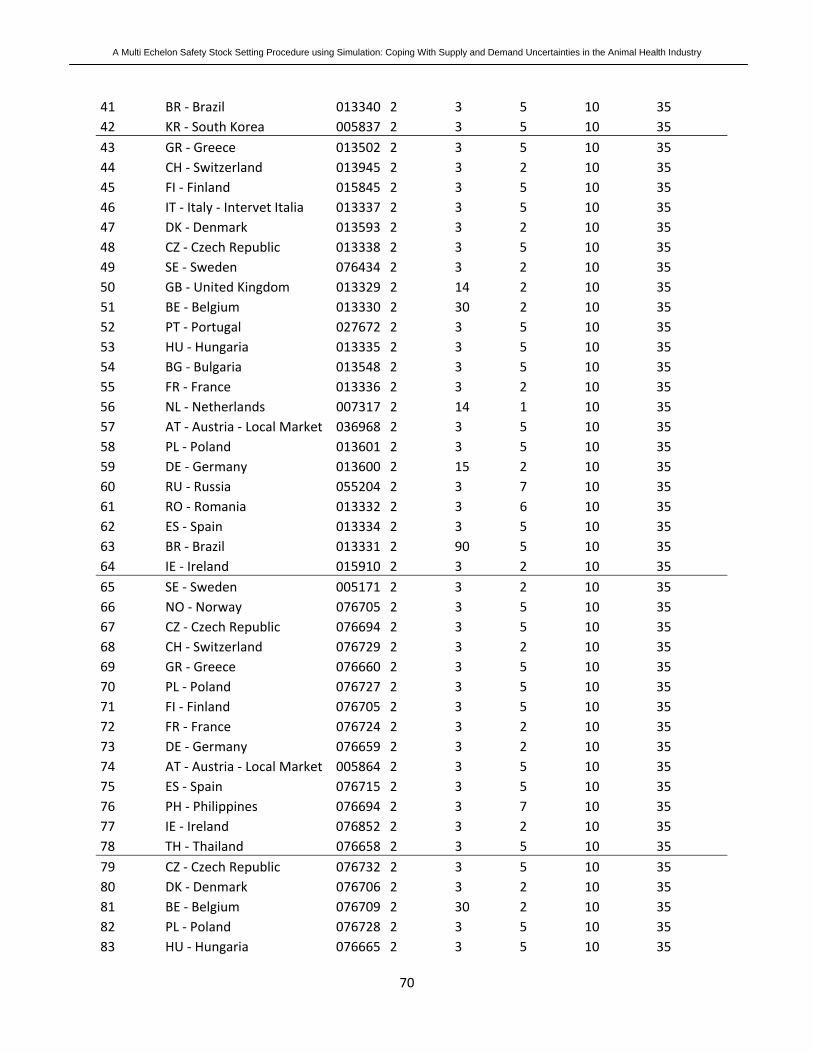
A Multi Echelon Safety Stock Setting Procedure using Simulation: Coping With Supply and Demand Uncertainties in the Animal Health Industry
70
41 BR ‐ Brazil 013340 2 3 5 10 35 42 KR ‐ South Korea 005837 2 3 5 10 35 43 GR ‐ Greece 013502 2 3 5 10 35 44 CH ‐ Switzerland 013945 2 3 2 10 35 45 FI ‐ Finland 015845 2 3 5 10 35 46 IT ‐ Italy ‐ Intervet Italia 013337 2 3 5 10 35 47 DK ‐ Denmark 013593 2 3 2 10 35 48 CZ ‐ Czech Republic 013338 2 3 5 10 35 49 SE ‐ Sweden 076434 2 3 2 10 35 50 GB ‐ United Kingdom 013329 2 14 2 10 35 51 BE ‐ Belgium 013330 2 30 2 10 35 52 PT ‐ Portugal 027672 2 3 5 10 35 53 HU ‐ Hungaria 013335 2 3 5 10 35 54 BG ‐ Bulgaria 013548 2 3 5 10 35 55 FR ‐ France 013336 2 3 2 10 35 56 NL ‐ Netherlands 007317 2 14 1 10 35 57 AT ‐ Austria ‐ Local Market 036968 2 3 5 10 35 58 PL ‐ Poland 013601 2 3 5 10 35 59 DE ‐ Germany 013600 2 15 2 10 35 60 RU ‐ Russia 055204 2 3 7 10 35 61 RO ‐ Romania 013332 2 3 6 10 35 62 ES ‐ Spain 013334 2 3 5 10 35 63 BR ‐ Brazil 013331 2 90 5 10 35 64 IE ‐ Ireland 015910 2 3 2 10 35 65 SE ‐ Sweden 005171 2 3 2 10 35 66 NO ‐ Norway 076705 2 3 5 10 35 67 CZ ‐ Czech Republic 076694 2 3 5 10 35 68 CH ‐ Switzerland 076729 2 3 2 10 35 69 GR ‐ Greece 076660 2 3 5 10 35 70 PL ‐ Poland 076727 2 3 5 10 35 71 FI ‐ Finland 076705 2 3 5 10 35 72 FR ‐ France 076724 2 3 2 10 35 73 DE ‐ Germany 076659 2 3 2 10 35 74 AT ‐ Austria ‐ Local Market 005864 2 3 5 10 35 75 ES ‐ Spain 076715 2 3 5 10 35 76 PH ‐ Philippines 076694 2 3 7 10 35 77 IE ‐ Ireland 076852 2 3 2 10 35 78 TH ‐ Thailand 076658 2 3 5 10 35 79 CZ ‐ Czech Republic 076732 2 3 5 10 35 80 DK ‐ Denmark 076706 2 3 2 10 35 81 BE ‐ Belgium 076709 2 30 2 10 35 82 PL ‐ Poland 076728 2 3 5 10 35 83 HU ‐ Hungaria 076665 2 3 5 10 35

A Multi Echelon Safety Stock Setting Procedure using Simulation: Coping With Supply and Demand Uncertainties in the Animal Health Industry
71
84 FR ‐ France 076725 2 3 2 10 35 85 DE ‐ Germany 076730 2 3 2 10 35 86 ES ‐ Spain 076716 2 3 5 10 35 87 BG ‐ Bulgaria 076993 2 3 5 10 35 88 TW ‐ Taiwan 076713 2 3 7 10 35 89 RU ‐ Russia 063644 2 3 7 10 35 90 IT ‐ Italy ‐ Intervet Italia 076707 2 3 5 10 35 91 PH ‐ Philippines 076993 2 3 7 10 35 92 RO ‐ Romania 076993 2 3 6 10 35 93 NL ‐ Netherlands 076832 2 14 1 10 35 94 BR ‐ Brazil 076711 2 90 5 10 35 95 A FPU 20 ML 002391 3 68 0 0 140 96 A FPU 50 ML 002392 3 68 0 0 140 97 A FPU 100 ML 002393 3 68 0 0 140 98 A FPU 250 ML Turkey 002389 3 75 0 0 136 99 A FPU 250 ML Pig 044595 3 75 0 0 136 100 Bio product Y FPU 20 ML 002396 3 82 0 0 140 101 Bio product Y FPU 50 ML 002395 3 82 0 0 140 102 B FPU 20 ML 003385 3 82 0 0 140 103 B FPU 50 ML 003384 3 82 0 0 140 104 A Bulk NL10 001997 3 0 0 0 35 105 A Bulk ES10 001997 3 0 0 0 0 106 Bio product Y Bulk 002394 3 0 0 0 35 107 B Bulk 002223 3 0 0 0 35 108 A M2 ANTIGEN NL10 002646 3 48 5 0 161 109 A M2 ANTIGEN GB10 002646 3 42 0 0 118 110 A M2 ANTIGEN ES10 002646 3 7 5 0 105 111 B antigen inact 002706 3 59 0 0 140 112 B before inact 002885 3 0 0 0 35

A Multi Echelon Safety Stock Setting Procedure using Simulation: Coping With Supply and Demand Uncertainties in the Animal Health Industry
72
D. GENERAL AND DEMAND UNCERTAINTY PARAMETERS BIO PRODUCT Y ComOp UIN Demand/w Sigma Beta Alpha Q Safety Stock 1 CH ‐ Switzerland 013610 30.10 24.77 20.38 1.48 540 100 2 SE ‐ Sweden 035629 20.73 42.23 86.04 0.24 540 94 3 CH ‐ Switzerland 013582 24.17 21.04 18.31 1.32 720 110 4 DK ‐ Denmark 013592 100.56 231.31 532.04 0.19 1800 600 5 FI ‐ Finland 013913 115.65 140.10 169.74 0.68 2040 500 6 IT ‐ Italy ‐ Intervet Italia 013314 178.52 134.29 101.01 1.77 2520 825 7 BE ‐ Belgium 013308 83.31 192.30 443.86 0.19 2160 1242 8 GR ‐ Greece 013313 25.27 37.63 56.03 0.45 720 120 9 AT ‐ Austria ‐ Local Market 038154 5.23 13.15 33.07 0.16 240 30 10 IE ‐ Ireland 015908 68.38 54.23 43.01 1.59 1800 300 11 DE ‐ Germany 013649 151.63 111.99 82.71 1.83 2880 604 12 FR ‐ France 013312 101.71 118.28 137.54 0.74 2400 400 13 GB ‐ United Kingdom 013307 397.67 374.25 352.22 1.13 5040 1600 14 NL ‐ Netherlands 007316 592.52 426.54 307.05 1.93 6840 2699 15 RO ‐ Romania 013309 25.71 55.65 120.45 0.21 960 400 16 CZ ‐ Czech Republic 013372 3.54 10.61 31.76 0.11 60 20 17 HU ‐ Hungaria 013311 146.46 411.05 1153.64 0.13 4920 1487 18 PL ‐ Poland 013316 580.31 237.48 97.18 5.97 9480 6000 19 ES ‐ Spain 013310 1070.40 1138.90 1211.78 0.88 8640 4538 20 DK ‐ Denmark 057267 48.92 170.71 595.77 0.08 1320 492 21 JP ‐ Japan 002393 513.67 153.73 46.01 11.16 12000 0 22 NL ‐ Netherlands 059503 226.00 49.85 11.00 20.55 3180 1029 23 GB ‐ United Kingdom 015689 222.23 441.06 875.38 0.25 2280 600 24 DK ‐ Denmark 020714 8.98 37.55 157.05 0.06 372 100 25 FR ‐ France 017516 102.69 106.25 109.93 0.93 1152 400 26 NL ‐ Netherlands 076667 29.00 34.44 40.91 0.71 1176 325 27 PL ‐ Poland 049398 96.65 454.36 2136.08 0.05 2628 2300 28 FI ‐ Finland 015844 265.85 147.50 81.83 3.25 2160 1125 29 CH ‐ Switzerland 013944 98.56 75.16 57.32 1.72 1350 500 30 GR ‐ Greece 013343 103.50 135.98 178.66 0.58 1350 500 31 NO ‐ Norway 043140 61.92 60.40 58.92 1.05 810 300 32 DK ‐ Denmark 005486 17.92 132.12 974.30 0.02 1350 359 33 SE ‐ Sweden 076433 101.04 79.86 63.12 1.60 1350 450 34 PT ‐ Portugal 027671 99.79 116.66 136.38 0.73 2160 567 35 PL ‐ Poland 013603 288.54 385.64 515.41 0.56 3240 2500 36 GB ‐ United Kingdom 013339 99.27 43.91 19.42 5.11 1620 400 37 FR ‐ France 013342 815.85 735.91 663.79 1.23 4860 3300 38 DE ‐ Germany 013602 134.56 208.30 322.45 0.42 2160 700 39 ES ‐ Spain 013341 175.27 541.60 1673.59 0.10 2700 922 40 BG ‐ Bulgaria 076094 9.31 10.29 11.38 0.82 270 55 41 BR ‐ Brazil 013340 16.79 28.44 48.15 0.35 200 67

A Multi Echelon Safety Stock Setting Procedure using Simulation: Coping With Supply and Demand Uncertainties in the Animal Health Industry
73
42 KR ‐ South Korea 005837 263.29 182.49 126.48 2.08 3780 1275 43 GR ‐ Greece 013502 69.63 92.41 122.66 0.57 720 300 44 CH ‐ Switzerland 013945 136.21 38.45 10.85 12.55 960 530 45 FI ‐ Finland 015845 125.35 74.57 44.36 2.83 960 450 46 IT ‐ Italy ‐ Intervet Italia 013337 382.81 189.78 94.09 4.07 1680 1584 47 DK ‐ Denmark 013593 443.75 1132.40 2889.76 0.15 2520 3334 48 CZ ‐ Czech Republic 013338 15.79 20.69 27.10 0.58 360 70 49 SE ‐ Sweden 076434 59.17 38.12 24.56 2.41 600 280 50 GB ‐ United Kingdom 013329 365.19 305.03 254.78 1.43 1800 1350 51 BE ‐ Belgium 013330 400.81 1288.34 4141.15 0.10 2160 3929 52 PT ‐ Portugal 027672 91.67 76.31 63.53 1.44 1320 480 53 HU ‐ Hungaria 013335 144.13 228.67 362.79 0.40 1560 945 54 BG ‐ Bulgaria 013548 41.42 51.13 63.12 0.66 960 260 55 FR ‐ France 013336 897.98 631.15 443.60 2.02 3600 3600 56 NL ‐ Netherlands 007317 912.60 163.31 29.23 31.23 5400 3123 57 AT ‐ Austria ‐ Local Market 036968 91.94 38.61 16.22 5.67 1200 420 58 PL ‐ Poland 013601 194.75 215.16 237.70 0.82 2280 2000 59 DE ‐ Germany 013600 1759.71 758.62 327.04 5.38 5160 10500 60 RU ‐ Russia 055204 373.21 254.32 173.30 2.15 3120 2709 61 RO ‐ Romania 013332 48.94 91.15 169.76 0.29 1080 720 62 ES ‐ Spain 013334 571.79 631.48 697.41 0.82 3960 3287 63 BR ‐ Brazil 013331 146.42 148.83 151.28 0.97 1800 900 64 IE ‐ Ireland 015910 147.79 138.88 130.50 1.13 1920 650 65 SE ‐ Sweden 005171 25.06 97.03 375.62 0.07 540 105 66 NO ‐ Norway 076705 34.52 58.62 99.54 0.35 810 150 67 CZ ‐ Czech Republic 076694 7.48 6.18 5.10 1.47 240 40 68 CH ‐ Switzerland 076729 27.40 22.52 18.51 1.48 540 100 69 GR ‐ Greece 076660 10.08 26.44 69.33 0.15 270 55 70 PL ‐ Poland 076727 7.10 48.78 334.93 0.02 1620 440 71 FI ‐ Finland 076705 23.69 93.13 366.16 0.06 540 100 72 FR ‐ France 076724 16.00 29.05 52.73 0.30 270 65 73 DE ‐ Germany 076659 28.92 63.72 140.41 0.21 540 109 74 AT ‐ Austria ‐ Local Market 005864 7.21 16.57 38.10 0.19 270 50 75 ES ‐ Spain 076715 39.79 78.81 156.09 0.25 810 133 76 PH ‐ Philippines 076694 42.50 38.44 34.76 1.22 1350 227 77 IE ‐ Ireland 076852 52.67 69.91 92.80 0.57 1080 200 78 TH ‐ Thailand 076658 701.98 948.67 1282.05 0.55 8370 4100 79 CZ ‐ Czech Republic 076732 6.63 26.93 109.50 0.06 240 40 80 DK ‐ Denmark 076706 636.98 430.15 290.48 2.19 2880 3100 81 BE ‐ Belgium 076709 63.06 79.90 101.24 0.62 960 634 82 PL ‐ Poland 076728 48.92 224.40 1029.44 0.05 600 110 83 HU ‐ Hungaria 076665 95.22 232.16 566.03 0.17 1440 734 84 FR ‐ France 076725 17.06 18.62 20.32 0.84 600 100

A Multi Echelon Safety Stock Setting Procedure using Simulation: Coping With Supply and Demand Uncertainties in the Animal Health Industry
74
85 DE ‐ Germany 076730 39.46 29.46 22.00 1.79 840 215 86 ES ‐ Spain 076716 84.63 84.74 84.86 1.00 840 231 87 BG ‐ Bulgaria 076993 5.19 17.24 57.28 0.09 120 25 88 TW ‐ Taiwan 076713 53.17 59.76 67.18 0.79 1680 600 89 RU ‐ Russia 063644 44.98 79.96 142.14 0.32 1080 300 90 IT ‐ Italy ‐ Intervet Italia 076707 61.04 91.09 135.93 0.45 840 334 91 PH ‐ Philippines 076993 76.27 112.30 165.35 0.46 1080 250 92 RO ‐ Romania 076993 26.23 145.11 802.83 0.03 1320 800 93 NL ‐ Netherlands 076832 480.81 260.46 141.10 3.41 5640 2000 94 BR ‐ Brazil 076711 23.94 23.75 23.57 1.02 360 210 95 A FPU 20 ML 002391 50.83 1000 500 96 A FPU 50 ML 002392 3671.02 23500 25000 97 A FPU 100 ML 002393 1010.81 12000 8500 98 A FPU 250 ML Turkey 002389 140.67 6000 1206 99 A FPU 250 ML Pig 044595 96.65 6000 829 100 Bio product Y FPU 20 ML 002396 2551.48 23000 25000 101 Bio product Y FPU 50 ML 002395 7421.05 23500 42500 102 B FPU 20 ML 003385 1024.40 20000 8500 103 B FPU 50 ML 003384 1763.57 23500 13500 104 A Bulk NL10 001997 300.01 1250 0 105 A Bulk ES10 001997 65.02 1000 0 106 Bio product Y Bulk 002394 449.45 1250 0 107 B Bulk 002223 116.80 1250 0 108 A M2 ANTIGEN NL10 002646 119.89 250 2056 109 A M2 ANTIGEN GB10 002646 6.50 200 0 110 A M2 ANTIGEN ES10 002646 6.50 200 112 111 B antigen inact 002706 102.04 480 1750 112 B before inact 002885 102.04 160 0

A Multi Echelon Safety Stock Setting Procedure using Simulation: Coping With Supply and Demand Uncertainties in the Animal Health Industry
75
E. SUPPLY UNCERTAINTY PARAMETERS BIO PRODUCT Y Test Repetition Bio product Y Batch Rejections Bio product Y Antigen B 3.00% Antigen A # of batches Percentage Antigen A NL10 3.00% rejected 11 1.92% Antigen A GB10 3.00% accepted 562 98.08% Bulk A 0.00% total 573 100.00% Bulk Bio product Y 0.00% Antigen B # of batches Percentage Bulk B 0.00% rejected 0 0.00% FPU A 20 ML 5.00% accepted 66 100.00% FPU A 50 ML 5.00% total 66 100.00% FPU A 100 ML 5.00% Bulk total # of batches Percentage FPU A 250 ML 5.00% rejected 0 0.00% FPU Bio product Y 20 ML 5.00% accepted 136 100.00% FPU Bio product Y 50 ML 5.00% Total 136 100.00% FPU B 20 ML 5.00% FPU # of batches Percentage FPU B 50 ML 5.00% rejected 8 3.21% FPP 0.00% accepted 241 96.79% Total 249 100.00% Batch value deviation Bio product Y FPP # of batches Percentage Antigen B ‐1.20% rejected 0 0.00% Antigen A NL10 ‐7.39% accepted 1,735 100.00% Antigen A GB10 5.03% Total 1,735 100.00% Bulk A ‐0.02% Bulk Bio product Y 0.03% Bulk B 0.01% Yield fluctuation A Antigen FPU A 20 ML 1.91% A Antigen NL10 ‐4.11% FPU A 50 ML ‐0.03% A Antigen GB10 ‐0.96% FPU A 100 ML ‐0.55% FPU Bio product Y 20 ML ‐0.10% FPU Bio product Y 50 ML 0.01% FPU B 20 ML ‐4.22% FPU B 50 ML ‐0.39% FPP ‐0.06%
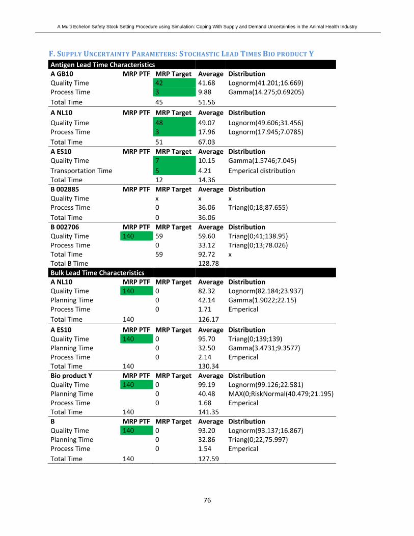
A Multi Echelon Safety Stock Setting Procedure using Simulation: Coping With Supply and Demand Uncertainties in the Animal Health Industry
76
F. SUPPLY UNCERTAINTY PARAMETERS: STOCHASTIC LEAD TIMES BIO PRODUCT Y Antigen Lead Time Characteristics A GB10 MRP PTF MRP Target Average Distribution Quality Time 42 41.68 Lognorm(41.201;16.669) Process Time 3 9.88 Gamma(14.275;0.69205) Total Time 45 51.56 A NL10 MRP PTF MRP Target Average Distribution Quality Time 48 49.07 Lognorm(49.606;31.456) Process Time 3 17.96 Lognorm(17.945;7.0785) Total Time 51 67.03 A ES10 MRP PTF MRP Target Average Distribution Quality Time 7 10.15 Gamma(1.5746;7.045) Transportation Time 5 4.21 Emperical distribution Total Time 12 14.36 B 002885 MRP PTF MRP Target Average Distribution Quality Time x x x Process Time 0 36.06 Triang(0;18;87.655) Total Time 0 36.06 B 002706 MRP PTF MRP Target Average Distribution Quality Time 140 59 59.60 Triang(0;41;138.95) Process Time 0 33.12 Triang(0;13;78.026) Total Time 59 92.72 x Total B Time 128.78 Bulk Lead Time Characteristics A NL10 MRP PTF MRP Target Average Distribution Quality Time 140 0 82.32 Lognorm(82.184;23.937) Planning Time 0 42.14 Gamma(1.9022;22.15) Process Time 0 1.71 Emperical Total Time 140 126.17 A ES10 MRP PTF MRP Target Average Distribution Quality Time 140 0 95.70 Triang(0;139;139) Planning Time 0 32.50 Gamma(3.4731;9.3577) Process Time 0 2.14 Emperical Total Time 140 130.34 Bio product Y MRP PTF MRP Target Average Distribution Quality Time 140 0 99.19 Lognorm(99.126;22.581) Planning Time 0 40.48 MAX(0;RiskNormal(40.479;21.195)Process Time 0 1.68 Emperical Total Time 140 141.35 B MRP PTF MRP Target Average Distribution Quality Time 140 0 93.20 Lognorm(93.137;16.867) Planning Time 0 32.86 Triang(0;22;75.997) Process Time 0 1.54 Emperical Total Time 140 127.59

A Multi Echelon Safety Stock Setting Procedure using Simulation: Coping With Supply and Demand Uncertainties in the Animal Health Industry
77
FPU Lead Time Characteristics A 20 ML MRP PTF MRP Target Average Distribution Quality Time 140 68 65.42857143 Gamma(42.702;1.5322) Planning Time 0 59 Lognorm(58.709;15.788) Process Time 3 1 Deterministic Total Time 140 125.4285714 A 50 ML MRP PTF MRP Target Average Distribution Quality Time 140 68 75.4137931 Gamma(11.997;6.2863) Planning Time 0 49.92682927 Gamma(3.3146;15.063) Process Time 3 1.317073171 Emperical Total Time 140 126.6576955 A 100 ML MRP PTF MRP Target Average Distribution Quality Time 140 68 83 Gamma(15.724;5.2784) Planning Time 0 57.58823529 Gamma(2.4709;23.307) Process Time 3 1.176470588 Emperical Total Time 140 141.7647059 A 250 ML (Turkey) MRP PTF MRP Target Average Distribution Quality Time 136 75 80.64285714 Weibull(2.3046;88.779) Planning Time 0 30.42857143 Lognorm(31.168;23.961) Process Time 3 3 Emperical Total Time 136 114.0714286 A 250 ML (PIG) MRP PTF MRP Target Average Distribution Quality Time 136 75 80.64285714 Weibull(2.3046;88.779) Planning Time 0 16.5 Emperical Process Time 3 2.666666667 Emperical Total Time 136 99.80952381 Bio product Y 20 ML MRP PTF MRP Target Average Distribution Quality Time 140 82 87.92307692 Weibull(2.2888;98.374) Planning Time 0 52.46666667 Gamma(2.2997;22.81) Process Time 3 1.733333333 Emperical Total Time 140 142.1230769 Bio product Y 50 ML MRP PTF MRP Target Average Distribution Quality Time 140 82 86.37335036 Triang(0;82;159.87) Planning Time 0 47.98571429 Weibull(2.0795;53.925) Process Time 3 1.242857143 Emperical Total Time 140 135.6019218 B 20 ML MRP PTF MRP Target Average Distribution Quality Time 140 82 96.1 Lognorm(95.974;24.261) Planning Time 0 45.15384615 Lognorm(45.193;27.312) Process Time 3 2.153846154 Emperical Total Time 140 143.4076923 B 50 ML MRP PTF MRP Target Average Distribution Quality Time 140 82 90.53333333 Triang(0;84;185.24) Planning Time 0 40.05555556 Gamma(3.8943;10.286) Process Time 3 1.333333333 Emperical Total Time 140 131.9222222

A Multi Echelon Safety Stock Setting Procedure using Simulation: Coping With Supply and Demand Uncertainties in the Animal Health Industry
78
FPP Lead Time Characteristics ES10 MRP PTF MRP Target Average Distribution Quality Time MRP value MRP value Deterministic Process Time 10 7.51 Gamma(4.2538;1.7649) Transportation Time MRP value MRP value Deterministic NL10 MRP PTF MRP Target Average Distribution Quality Time MRP value MRP value Deterministic Process Time 10 12.88 Lognorm(12.87;4.6796) Transportation Time MRP value MRP value Deterministic

A Multi Echelon Safety Stock Setting Procedure using Simulation: Coping With Supply and Demand Uncertainties in the Animal Health Industry
79
APPENDIX VII: LIST OF DEFINITIONS Backlog = In case Physical Inventory does not allow a customer order to be satisfied directly and the customer is willing to wait there is a backlog
Inventory Position = Physical Inventory – Backlog + Scheduled Productions
Lead Time = The time between the placement of an order and the order being ready for the next phase
Physical Inventory = Physical available and free stock. This value can never be negative.

A Multi Echelon Safety Stock Setting Procedure using Simulation: Coping With Supply and Demand Uncertainties in the Animal Health Industry
80
APPENDIX VIII: LIST OF SYMBOLS αfpp = Scale parameter of Gamma distribution of end item fpp βfpp = Shape parameter of Gamma distribution of end item fpp AOQfpp(t) = Actual Order Quantity of end item fpp determined in period t AOQfpu(t) = Actual Order Quantity of Finished Product Unpacked fpu determined in period t AOQrm(t) = Actual Order Quantity of API or Antigen rm determined in period t
)(tAOQDfpu = Actual Order Quantity with batch deviation of Finished Product Unpacked fpu in period t
APQfpu = Actual Production Quantity of Finished Product Unpacked fpu ARQfpu = Actual Reduction Quantity of Finished Product Unpacked fpu Bfpp(t) = Backlog in units of end item fpp at the end of period t Bfpu(t) = Backlog in units of Finished Product Unpacked fpu at the end ofperiod t Brm(t) = Backlog in units of API or Antigen rm at the end of period t BFfpu = BOM factor of Finished Product Unpacked fpu BFfpu’ = BOM factor of other Finished Product Unpacked fpu’ using the similar Bulk BFrm = BOM factor of API or Antigen rm CPfpp = Cost price of end item fpp CPfpu = Cost price of Finished Product Unpacked fpu CPrm = Cost price of API or Antigen rm Dfpp(t) = Demand for end item fpp in period t
fppD = Average demand per week of end item fpp LTfppD = Demand during lead time of end item fpp in period t
LTfpuD = Demand during lead time of Finished Product Unpacked fpu in period t
LTrmD = Demand during lead time of API or Antigen rm in period t
Dvfpu(t) = Batch value deviation of Finished Product Unpacked fpu in period t Dvrm(t) = Batch value deviation of Antigen rm in period t FA = Forecast Accuracy FPP = Number of end items (FPPs) FPU = Number of Finished Product Unpacked(FPUs) FQbulk = Fixed Quantity of Bulk product Bulk FR = Fill rate = service level IPfpp(t) = Inventory Position of end item fpp in period t IPfpu(t) = Inventory Position of Finished Product Unpacked fpu in period t IPrm(t) = Inventory Position of API or Antigen rm in period t OOfpp(t) = Amount of Outstanding Orders of end item fpp in period t OOfpu(t) = Amount of Outstanding Orders of Finished Product Unpacked fpu in period t ORfpu(t) = Amount of Orders Released of Finished Product Unpacked fpu in period t

A Multi Echelon Safety Stock Setting Procedure using Simulation: Coping With Supply and Demand Uncertainties in the Animal Health Industry
81
PIfpp(t) = Physical Inventory of end item fpp in period t PIfpu(t) = Physical Inventory of Finished Product Unpacked fpu in period t PIrm(t) = Physical Inventory of API or Antigen rm in period t
fppPI = Average Physical Inventory of end item fpp over all simulation periods
fpuPI = Average Physical Inventory of Finished Product Unpacked fpu over all simulation periods
rmPI = Average Physical Inventory of API or Antigen rm over all simulation periods PLTfpp = Planning Time (MRP planning time) of end item fpp PLTfpu = Planning Time (MRP planning time) of Finished Product Unpacked fpu PTfpp = Production Time (MRP planning time) of end item fpp PTfpu = Production Time (MRP planning time) of Finished Product Unpacked fpu PTrm = Production Time (MRP planning time) of API or Antigen rm Qbulk = Batch size (Order Quantity) of Bulk product Bulk Qfpp = Batch size (Order Quantity) of end item fpp Qfpu = Batch size (Order Quantity) of Finished Product Unpacked fpu Qrm = Batch size (Order Quantity) of API or Antigen rm Qfpp(t) = Order Quantity of end item fpp in period t Qfpu(t) = Order Quantity of Finished Product Unpacked fpu in period t Qrm(t) = Order Quantity of API or Antigen rm in period t QUfpp(t) = Quantity Used of end item fpp in period t QUfpu(t) = Quantity Used of Finished Product Unpacked fpu in period t QSfpp(t) = Quantity Shipped of end item fpp in period t QTfpp = Quality Test Time (MRP planning time) of end item fpp QTfpu = Quality Test Time (MRP planning time) of Finished Product Unpacked fpu QTrm = Quality Test Time (MRP planning time) of API or Antigen rm RM = Number of APIs or Antigens ROQfpu(t) = Rest Order Quantity of Finished Product Unpacked fpu in period t
)(tROQDfpu = Rest Order Quantity with batch deviation of Finished Product Unpacked fpu in period t
SPfpp = Sales price of end item fpp SSfpp = Safety stock of end item fpp SSfpu = Safety stock of Finished Product Unpacked fpu SSrm = Safety stock of API or Antigen rm t = time period (weekly time bucket) T = number of time periods used in simulation model TTfpp = Transportation Time (MRP planning time) of end item fpp TTrm = Transportation Time (MRP planning time) of API rm WIPfpp (t) = Work In Process of end item fpp in period t WIPfpu (t) = Work In Process of Finished Product Unpacked fpu in period t WIPrm (t) = Work In Process of API or Antigen rm in period t
fppWIP = Average Work In Process of end item fpp over all simulation periods

A Multi Echelon Safety Stock Setting Procedure using Simulation: Coping With Supply and Demand Uncertainties in the Animal Health Industry
82
fpuWIP = Average Work In Process of Finished Product Unpacked fpu over all simulation periods
rmWIP = Average Work In Process of API or Antigen rm over all simulation periods Yrm(t) = Yield fluctuation of Antigen rm in period t
A Multi Echelon Safety Stock Setting Procedure using Simulation: Coping With Supply and Demand Uncertainties in the Animal Health Industry
83
APPENDIX IX: SIMULATION PARAMETERS:
Before simulation of the model can take place, a number of parameters need to be set. First, the warm‐up period needs to be determined to prevent any possible bias due to initial parameter settings. Since we have assumed in chapter 6 that this simulation study concerns a steady state simulation, we need to find a point in time where the state of the simulation is independent of the initial start‐up conditions. Moreover, the number of replications and the run length which are required to yield significant and unbiased results should be determined. A pilot run is used to determine these three parameters. According to Law and Kelton (2000) a pilot run of at least 5 replications and a large run length is the correct input to yield significant results. Therefore, we have used 5 replications and a run length of 13,000 weeks during the pilot run. The performance measured will be the amount of backorders in dollar volume. We have selected this performance measure since the backorder volume is directly related to the service level. However, we are aware of the fact that the backorder volumes are often equal to zero, which might have an impact on the parameters determined.
Warm up period The Welsh’s method as described in Law and Kelton (2000), is used to determine the warm up period of the simulation. 5 replications of the simulation, each with a length of 13,000 weeks are conducted to determine this warm up period. Let Yji be the ith observation form the jth replication (j = 1,2,…..,n; i = 1, 2, ….., m)
Let ∑ ==
n
j jii nYY1
/ for i = 1,2,…, m
Then )(wYi is the moving average with window w (w is a positive integer such that w ≤ (m/4)).
According to Law and Kelton (2000), the following holds for the moving average:
wiifi
YwY
wmwiifw
YwY
i
issi
i
w
wssi
i
,...,1_12
)(
,...,1_12
)(
1
)1( =−
=
−+=+
=
∑
∑
−
−−=
+
−=
+
For three levels of w ({1,200; 2,000; 3,300}), 5 replications with 13,000 weeks each are executed. The resulting graphs are shown in Figure 1, Figure 2 and Figure 3.
A Multi Echelon Safety Stock Setting Procedure using Simulation: Coping With Supply and Demand Uncertainties in the Animal Health Industry
84
Figure 1: Moving average backorders (w = 1200)
Figure 2: Moving average backorders (w = 2000)
0
10
20
30
40
50
60
70
1 305 609 913 12171521182521292433273730413345364939534257456148655169547357776081638566896993729776017905820985138817912194259729100331033710641109451124911553
0
10
20
30
40
50
60
70
1 601 12011801240130013601420148015401600166017201780184019001960110201108011140112001
A Multi Echelon Safety Stock Setting Procedure using Simulation: Coping With Supply and Demand Uncertainties in the Animal Health Industry
85
Figure 3: Moving average backorders (w = 3300)
The window needs to be relatively high, since the backorder volume is zero most of the times and therefore a large window is necessary to determine the moving average. All graphs indicate that the backorder volume smoothens out around 2,500 weeks. Therefore we have selected a warm up period of 2,500 weeks.
Simulation run length Law and Kelton (2000) suggest a simulation run length that is large relative to the warm‐up period; Law and Kelton give an example of a simulation with a warm up period of 24 time units and a run length of 160 which they call sufficient. Therefore, it is assumed that, with a warm‐up of 2,500 weeks, simulating with a run length of 25,000 weeks will be more than sufficient to gain meaningful results.
Number of replications To determine the number of replications that will be used in the simulation, first the desired level of relative error, γ, as defined by Law and Kelton (2000) must be set. This relative error is the expected amount of relative average difference between the values of the replication means and the actual mean, μ. For this experiment the relative error will be set at 0.1 with a confidence level (1 – α) of 90%, which
means an α of 10% will be used. Using these settings means that X will have a relative error of at most γ/(1 – γ), “the adjusted relative error needed to get an actual relative error of γ” (Law and Kelton, 2000, p. 513), which is equal to 0.09 in about 90% of the cases, in 10% of the cases the relative error is larger.
To determine the number of replications required to yield the desired level of γ, Law and Kelton (2000) provide an approximate expression for the number of replications using the following data from the pilot run:
S2 (n) = population variance of the pilot run = 1.862191
0
10
20
30
40
50
60
70
1 601 1201 1801 2401 3001 3601 4201 4801 5401 6001 6601 7201 7801 8401 9001 96011020110801
A Multi Echelon Safety Stock Setting Procedure using Simulation: Coping With Supply and Demand Uncertainties in the Animal Health Industry
86
)(nX = average amount of backorders in dollar volume of the pilot run = 12.04687 n = number of replications in the pilot run = 5 The approximate number of replications required to obtain an estimate of μ (the actual backorder volume of the model) with a relative error of 0.1 and a confidence level of 90% is given by the following formula:
⎪⎪⎭
⎪⎪⎬
⎫
⎪⎪⎩
⎪⎪⎨
⎧
≤≥=−−
')(
)(
:min)(
2
2/1,1* γγ
α
nXinSt
nini
r
In which:
)(* γrn = the approximate number of replications required
2/1,1 α−−it = t distribution for 1 – α/2 (0.95) and i – 1 degrees of freedom
The colon “:” is read “such that” The smallest integer i that satisfies this equation is the approximate number of replications required. For the results from the pilot run this yields:
9'09,012.04687
862191.1
:5min)10.0(95,0,1
* =
⎪⎪⎭
⎪⎪⎬
⎫
⎪⎪⎩
⎪⎪⎨
⎧
≤≥=− i
tin
i
r
This means that the simulation will constitute of 9 replications of 25,000 weeks with a warm up period of 2,500 weeks.

A Multi Echelon Safety Stock Setting Procedure using Simulation: Coping With Supply and Demand Uncertainties in the Animal Health Industry
87
APPENDIX X: DESIGN MATRICES FOR FULL FACTORIAL DESIGN
Table 7.2: Scenario 2: Design Matrix for full(24) factorial design Factor number
Design point 1 2 3 4
1 ‐ ‐ ‐ ‐ 2 + ‐ ‐ ‐ 3 ‐ + ‐ ‐ 4 + + ‐ ‐ 5 ‐ ‐ + ‐ 6 + ‐ + ‐ 7 ‐ + + ‐ 8 + + + ‐ 9 ‐ ‐ ‐ + 10 + ‐ ‐ + 11 ‐ + ‐ + 12 + + ‐ + 13 ‐ ‐ + + 14 + ‐ + + 15 ‐ + + +
16 + + + +

A Multi Echelon Safety Stock Setting Procedure using Simulation: Coping With Supply and Demand Uncertainties in the Animal Health Industry
88
Table 7.2: Scenario 2: Design Matrix for full(26) factorial design
Factor number
Factor number
Design point 1 2 3 4 5 6 Design point 1 2 3 4 5 1 ‐ ‐ ‐ ‐ ‐ ‐ 33 ‐ ‐ ‐ ‐ ‐ +2 + ‐ ‐ ‐ ‐ ‐ 34 + ‐ ‐ ‐ ‐ +3 ‐ + ‐ ‐ ‐ ‐ 35 ‐ + ‐ ‐ ‐ +4 + + ‐ ‐ ‐ ‐ 36 + + ‐ ‐ ‐ +5 ‐ ‐ + ‐ ‐ ‐ 37 ‐ ‐ + ‐ ‐ +6 + ‐ + ‐ ‐ ‐ 38 + ‐ + ‐ ‐ +7 ‐ + + ‐ ‐ ‐ 39 ‐ + + ‐ ‐ +8 + + + ‐ ‐ ‐ 40 + + + ‐ ‐ +9 ‐ ‐ ‐ + ‐ ‐ 41 ‐ ‐ ‐ + ‐ +10 + ‐ ‐ + ‐ ‐ 42 + ‐ ‐ + ‐ +11 ‐ + ‐ + ‐ ‐ 43 ‐ + ‐ + ‐ +12 + + ‐ + ‐ ‐ 44 + + ‐ + ‐ +13 ‐ ‐ + + ‐ ‐ 45 ‐ ‐ + + ‐ +14 + ‐ + + ‐ ‐ 46 + ‐ + + ‐ +15 ‐ + + + ‐ ‐ 47 ‐ + + + ‐ +16 + + + + ‐ ‐ 48 + + + + ‐ +17 ‐ ‐ ‐ ‐ + ‐ 49 ‐ ‐ ‐ ‐ + +18 + ‐ ‐ ‐ + ‐ 50 + ‐ ‐ ‐ + +19 ‐ + ‐ ‐ + ‐ 51 ‐ + ‐ ‐ + +20 + + ‐ ‐ + ‐ 52 + + ‐ ‐ + +21 ‐ ‐ + ‐ + ‐ 53 ‐ ‐ + ‐ + +22 + ‐ + ‐ + ‐ 54 + ‐ + ‐ + +23 ‐ + + ‐ + ‐ 55 ‐ + + ‐ + +24 + + + ‐ + ‐ 56 + + + ‐ + +25 ‐ ‐ ‐ + + ‐ 57 ‐ ‐ ‐ + + +26 + ‐ ‐ + + ‐ 58 + ‐ ‐ + + +27 ‐ + ‐ + + ‐ 59 ‐ + ‐ + + +28 + + ‐ + + ‐ 60 + + ‐ + + +29 ‐ ‐ + + + ‐ 61 ‐ ‐ + + + +30 + ‐ + + + ‐ 62 + ‐ + + + +31 ‐ + + + + ‐ 63 ‐ + + + + +32 + + + + + ‐ 64 + + + + + +

A Multi Echelon Safety Stock Setting Procedure using Simulation: Coping With Supply and Demand Uncertainties in the Animal Health Industry
89
APPENDIX XI: RESULTS DETERMINATION HEURISTIC We have developed a heuristic which is used to determine the ‘optimal’ safety stock levels for the various simulation studies. To answer each sub question we have conducted several simulation runs and the heuristic will attempt to minimize the total inventory costs given the service level requirement. First, the performance given the current Intervet / S‐P A.H. safety stock settings is determined. Afterwards the optimization heuristic to minimize the total inventory costs starts. The process starts with the optimization of the safety stock at the most downstream stock point (FPP). Afterwards, combinations of stock points (e.g. API and FPP) are changed (one is increased with 5%, while the other is decreased until the performance of e.g. 94% is reached) and the third stock point remains unchanged. When the total inventory cost difference between the new situation and the old situation is lower than $5,000 (i.e. the total inventory costs in the new situation are less than $5,000 lower than in the old situation), we will move on to the next step in the heuristic. When the cost difference is higher than $5,000, this step is beneficial for the total inventory costs and will therefore be repeated. We have selected the 5% and $5,000 values, since using lower values would result in too detailed punctuality. A tradeoff between time/effort and impact on cost has been made at the beginning of the optimization process and trail optimizations indicated that using these values resulted in the highest effort reduction ratio. This process is continued until the fine‐tune phase is reached. In this phase the safety stock levels at the three controlled stock points are changed slightly(1%) and when this results in a decrease of inventory costs of more than $2,000, this phase will be repeated. If the decrease is less than $2,000 or when there is an increase, the safety stock levels are set back to the former levels and another fine tune combination is used. This is done three times and afterwards the heuristic optimal safety stock allocation is found. This fine‐tune phase is used to further optimize the values found. The 1% and $2,000 values are used to find a more detailed optimum.

A Multi Echelon Safety Stock Setting Procedure using Simulation: Coping With Supply and Demand Uncertainties in the Animal Health Industry
90
Heuristic for safety stock optimization
APPENDIX XIIA: RESULTS PHARMA PRODUCT X
CURRENT SITUATION INTERVET / SP A.H.
Intervet situation Pharma product X ($) API FPU FPP Total Safety Stock $ 293,424.74 $ 69,125.00 $ 118,460.83 $ 481,010.57 Average Quality Stock $ 67,585.64 $ 98,989.11 $ 7,843.91 $ 174,418.66 Average Released Stock $ 310,542.48 $ 108,815.00 $ 276,766.30 $ 696,123.78 Average Total Inventory $ 378,128.12 $ 207,804.12 $ 284,610.21 $ 870,542.45 Intervet situation Pharma product X (Log MoS) API FPU FPP Total Safety Stock [MoS] 9.00 MoS 1.05 MoS 1.50 MoS 11.54 MoSAverage WIP [MoS] 2.07 MoS 1.50 MoS 0.10 MoS 3.67 MoSAverage Physical Inventory [MoS] 9.52 MoS 1.65 MoS 3.51 MoS 14.68 MoSAverage Total Inventory [MoS] 11.59 MoS 3.14 MoS 3.61 MoS 18.35 MoS Intervet situation Pharma product X (Fin API FPU FPP Total
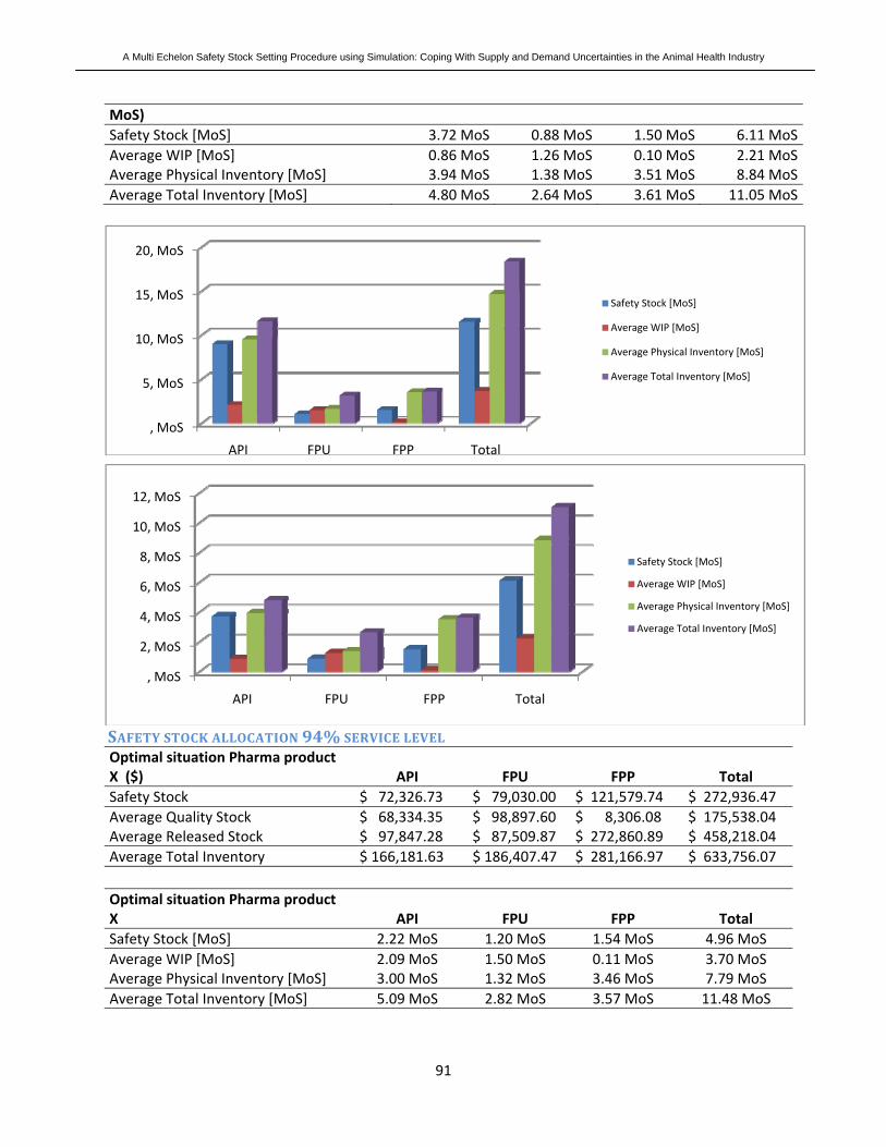
A Multi Echelon Safety Stock Setting Procedure using Simulation: Coping With Supply and Demand Uncertainties in the Animal Health Industry
91
MoS) Safety Stock [MoS] 3.72 MoS 0.88 MoS 1.50 MoS 6.11 MoSAverage WIP [MoS] 0.86 MoS 1.26 MoS 0.10 MoS 2.21 MoSAverage Physical Inventory [MoS] 3.94 MoS 1.38 MoS 3.51 MoS 8.84 MoSAverage Total Inventory [MoS] 4.80 MoS 2.64 MoS 3.61 MoS 11.05 MoS
SAFETY STOCK ALLOCATION 94% SERVICE LEVEL Optimal situation Pharma product X ($) API FPU FPP Total Safety Stock $ 72,326.73 $ 79,030.00 $ 121,579.74 $ 272,936.47 Average Quality Stock $ 68,334.35 $ 98,897.60 $ 8,306.08 $ 175,538.04 Average Released Stock $ 97,847.28 $ 87,509.87 $ 272,860.89 $ 458,218.04 Average Total Inventory $ 166,181.63 $ 186,407.47 $ 281,166.97 $ 633,756.07 Optimal situation Pharma product X API FPU FPP Total Safety Stock [MoS] 2.22 MoS 1.20 MoS 1.54 MoS 4.96 MoS Average WIP [MoS] 2.09 MoS 1.50 MoS 0.11 MoS 3.70 MoS Average Physical Inventory [MoS] 3.00 MoS 1.32 MoS 3.46 MoS 7.79 MoS Average Total Inventory [MoS] 5.09 MoS 2.82 MoS 3.57 MoS 11.48 MoS
, MoS
5, MoS
10, MoS
15, MoS
20, MoS
API FPU FPP Total
Safety Stock [MoS]
Average WIP [MoS]
Average Physical Inventory [MoS]
Average Total Inventory [MoS]
, MoS
2, MoS
4, MoS
6, MoS
8, MoS
10, MoS
12, MoS
API FPU FPP Total
Safety Stock [MoS]
Average WIP [MoS]
Average Physical Inventory [MoS]
Average Total Inventory [MoS]

A Multi Echelon Safety Stock Setting Procedure using Simulation: Coping With Supply and Demand Uncertainties in the Animal Health Industry
92
Optimal situation Pharma product X API FPU FPP Total Safety Stock [MoS] 0.92 MoS 1.00 MoS 1.54 MoS 3.46 MoS Average WIP [MoS] 0.87 MoS 1.26 MoS 0.10 MoS 2.23 MoS Average Physical Inventory [MoS] 1.24 MoS 1.11 MoS 3.46 MoS 5.82 MoS Average Total Inventory [MoS] 2.11 MoS 2.37 MoS 3.57 MoS 8.05 MoS
, MoS
2, MoS
4, MoS
6, MoS
8, MoS
10, MoS
12, MoS
API FPU FPP Total
Safety Stock [MoS]
Average WIP [MoS]
Average Physical Inventory [MoS]
Average Total Inventory [MoS]
, MoS
1, MoS
2, MoS
3, MoS
4, MoS
5, MoS
6, MoS
7, MoS
8, MoS
9, MoS
API FPU FPP Total
Safety Stock [MoS]
Average WIP [MoS]
Average Physical Inventory [MoS]
Average Total Inventory [MoS]

A Multi Echelon Safety Stock Setting Procedure using Simulation: Coping With Supply and Demand Uncertainties in the Animal Health Industry
93
SAFETY STOCK ALLOCATION 98% SERVICE LEVEL Optimal situation Pharma product X ($) API FPU FPP Total Safety Stock $ 103,274.33 $ 92,295.00 $ 295,717.13 $ 491,286.46 Average Quality Stock $ 67,105.00 $ 99,812.81 $ 7,629.86 $ 174,547.67 Average Released Stock $ 123,511.71 $ 127,068.25 $ 432,757.77 $ 683,337.72 Average Total Inventory $ 190,616.71 $ 226,881.05 $ 440,387.63 $ 857,885.39 Optimal situation Pharma product X API FPU FPP Total Safety Stock [MoS] 3.17 MoS 1.40 MoS 3.75 MoS 8.32 MoSAverage WIP [MoS] 2.06 MoS 1.51 MoS 0.10 MoS 3.66 MoSAverage Physical Inventory [MoS] 3.79 MoS 1.92 MoS 5.49 MoS 11.20 MoSAverage Total Inventory [MoS] 5.84 MoS 3.43 MoS 5.59 MoS 14.87 MoS Optimal situation Pharma product X API FPU FPP Total Safety Stock [MoS] 1.31 MoS 1.17 MoS 3.75 MoS 6.24 MoSAverage WIP [MoS] 0.85 MoS 1.27 MoS 0.10 MoS 2.22 MoSAverage Physical Inventory [MoS] 1.57 MoS 1.61 MoS 5.49 MoS 8.67 MoSAverage Total Inventory [MoS] 2.42 MoS 2.88 MoS 5.59 MoS 10.89 MoS
$‐
$100.000,00
$200.000,00
$300.000,00
$400.000,00
$500.000,00
$600.000,00
$700.000,00
API FPU FPP Total
Safety Stock [$]
Average Quality Stock (WIP) [$]
Average Released Stock (PI) [$]
Average Total Inventory [$]
$‐$100.000,00 $200.000,00 $300.000,00 $400.000,00 $500.000,00 $600.000,00 $700.000,00 $800.000,00 $900.000,00
$1.000.000,00
API FPU FPP Total
Safety Stock [$]
Average Quality Stock (WIP) [$]
Average Released Stock (PI) [$]
Average Total Inventory [$]

A Multi Echelon Safety Stock Setting Procedure using Simulation: Coping With Supply and Demand Uncertainties in the Animal Health Industry
94
, MoS
5, MoS
10, MoS
15, MoS
API FPU FPP Total
Safety Stock [MoS]
Average WIP [MoS]
Average Physical Inventory [MoS]
Average Total Inventory [MoS]
, MoS
2, MoS
4, MoS
6, MoS
8, MoS
10, MoS
12, MoS
API FPU FPP Total
Safety Stock [MoS]
Average WIP [MoS]
Average Physical Inventory [MoS]
Average Total Inventory [MoS]
$103.274,33 ; 21%
$92.295,00 ; 19%
$295.717,13 ; 60%
98% situation
API
FPU
FPP
$‐
$100.000,00
$200.000,00
$300.000,00
$400.000,00
$500.000,00
API FPU FPP Total94% situation $72.326,73 $79.030,00 $121.579,74 $272.936,47
Intervet situation $293.424,74 $69.125,00 $118.460,83 $481.010,57
98% situation $103.274,33 $92.295,00 $295.717,13 $491.286,46
Safety Stock volum
e
Safety Stock Allocation
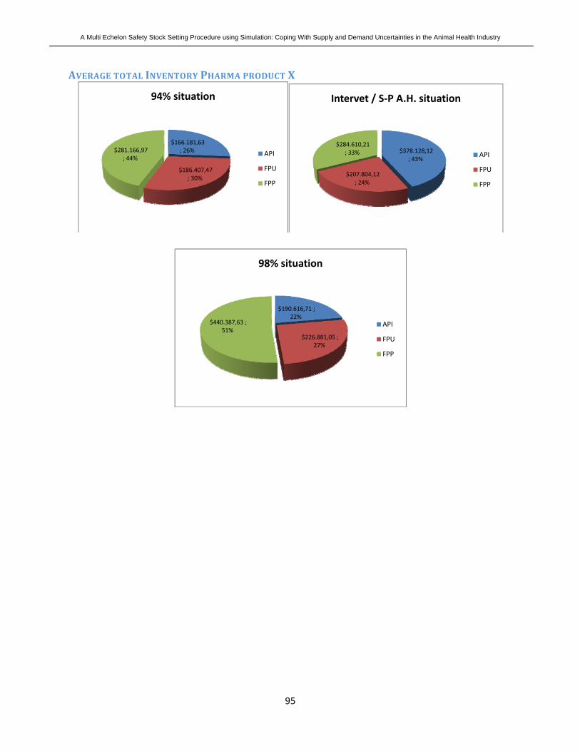
A Multi Echelon Safety Stock Setting Procedure using Simulation: Coping With Supply and Demand Uncertainties in the Animal Health Industry
95
AVERAGE TOTAL INVENTORY PHARMA PRODUCT X
$166.181,63 ; 26%
$186.407,47 ; 30%
$281.166,97 ; 44%
94% situation
API
FPU
FPP
$378.128,12 ; 43%
$207.804,12 ; 24%
$284.610,21 ; 33%
Intervet / S‐P A.H. situation
API
FPU
FPP
$190.616,71 ; 22%
$226.881,05 ; 27%
$440.387,63 ; 51%
98% situation
API
FPU
FPP
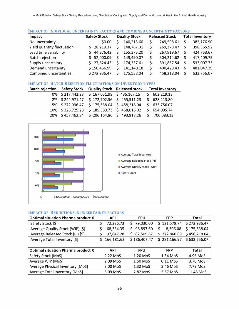
A Multi Echelon Safety Stock Setting Procedure using Simulation: Coping With Supply and Demand Uncertainties in the Animal Health Industry
96
IMPACT OF INDIVIDUAL UNCERTAINTY FACTORS AND COMBINED UNCERTAINTY FACTORS Impact Safety Stock Quality Stock Released Stock Total Inventory No uncertainty $0.00 $ 140,215.60 $ 249,598.61 $ 382,176.90 Yield quantity fluctuation $ 28,219.37 $ 148,767.31 $ 269,378.47 $ 398,365.92 Lead time variability $ 44,376.42 $ 155,375.20 $ 267,919.67 $ 424,753.67 Batch rejection $ 52,000.09 $ 149,490.07 $ 304,214.62 $ 417,409.75 Supply uncertainty $ 127,624.43 $ 174,337.61 $ 391,867.54 $ 533,007.73 Demand uncertainty $ 150,456.99 $ 141,140.18 $ 400,429.43 $ 481,047.39 Combined uncertainties $ 272,936.47 $ 175,538.04 $ 458,218.04 $ 633,756.07
IMPACT OF BATCH REJECTION FLUCTUATIONS ON INVENTORY TYPES Batch rejection Safety Stock Quality Stock Released stock Total Inventory
0% $ 217,442.23 $ 167,051.98 $ 435,167.15 $ 602,219.13 2% $ 244,971.47 $ 172,702.56 $ 455,511.23 $ 628,213.80 5% $ 272,936.47 $ 175,538.04 $ 458,218.04 $ 633,756.07
10% $ 326,725.28 $ 185,389.73 $ 468,616.02 $ 654,005.74 20% $ 457,462.84 $ 206,164.86 $ 493,918.26 $ 700,083.13
IMPACT OF REDUCTIONS IN UNCERTAINTY FACTORS Optimal situation Pharma product X API FPU FPP Total Safety Stock [$] $ 72,326.73 $ 79,030.00 $ 121,579.74 $ 272,936.47 Average Quality Stock (WIP) [$] $ 68,334.35 $ 98,897.60 $ 8,306.08 $ 175,538.04 Average Released Stock (PI) [$] $ 97,847.28 $ 87,509.87 $ 272,860.89 $ 458,218.04 Average Total Inventory [$] $ 166,181.63 $ 186,407.47 $ 281,166.97 $ 633,756.07 Optimal situation Pharma product X API FPU FPP Total Safety Stock [MoS] 2.22 MoS 1.20 MoS 1.54 MoS 4.96 MoS Average WIP [MoS] 2.09 MoS 1.50 MoS 0.11 MoS 3.70 MoS Average Physical Inventory [MoS] 3.00 MoS 1.32 MoS 3.46 MoS 7.79 MoS Average Total Inventory [MoS] 5.09 MoS 2.82 MoS 3.57 MoS 11.48 MoS
$‐ $300.000,00 $600.000,00 $900.000,00
0%
2%
5%
10%
20%
Average Total Inventory
Average Released stock (PI)
Average Quality Stock (WIP)
Safety Stock
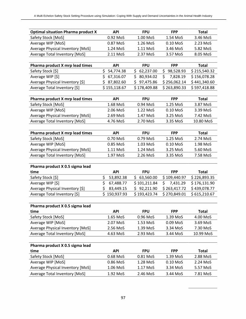
A Multi Echelon Safety Stock Setting Procedure using Simulation: Coping With Supply and Demand Uncertainties in the Animal Health Industry
97
Optimal situation Pharma product X API FPU FPP Total Safety Stock [MoS] 0.92 MoS 1.00 MoS 1.54 MoS 3.46 MoS Average WIP [MoS] 0.87 MoS 1.26 MoS 0.10 MoS 2.23 MoS Average Physical Inventory [MoS] 1.24 MoS 1.11 MoS 3.46 MoS 5.82 MoS Average Total Inventory [MoS] 2.11 MoS 2.37 MoS 3.57 MoS 8.05 MoS Pharma product X mrp lead times API FPU FPP Total Safety Stock [$] $ 54,774.38 $ 62,237.00 $ 98,528.93 $ 215,540.32 Average WIP [$] $ 67,316.07 $ 80,934.02 $ 7,828.19 $ 156,078.28 Average Physical Inventory [$] $ 87,802.60 $ 97,475.86 $ 256,062.14 $ 441,340.60 Average Total Inventory [$] $ 155,118.67 $ 178,409.88 $ 263,890.33 $ 597,418.88 Pharma product X mrp lead times API FPU FPP Total Safety Stock [MoS] 1.68 MoS 0.94 MoS 1.25 MoS 3.87 MoS Average WIP [MoS] 2.06 MoS 1.22 MoS 0.10 MoS 3.39 MoS Average Physical Inventory [MoS] 2.69 MoS 1.47 MoS 3.25 MoS 7.42 MoS Average Total Inventory [MoS] 4.76 MoS 2.70 MoS 3.35 MoS 10.80 MoS Pharma product X mrp lead times API FPU FPP Total Safety Stock [MoS] 0.70 MoS 0.79 MoS 1.25 MoS 2.74 MoS Average WIP [MoS] 0.85 MoS 1.03 MoS 0.10 MoS 1.98 MoS Average Physical Inventory [MoS] 1.11 MoS 1.24 MoS 3.25 MoS 5.60 MoS Average Total Inventory [MoS] 1.97 MoS 2.26 MoS 3.35 MoS 7.58 MoS Pharma product X 0.5 sigma lead time API FPU FPP Total Safety Stock [$] $ 53,892.38 $ 63,560.00 $ 109,440.97 $ 226,893.35 Average WIP [$] $ 67,488.77 $ 101,211.84 $ 7,431.29 $ 176,131.90 Average Physical Inventory [$] $ 83,449.15 $ 92,211.90 $ 263,417.72 $ 439,078.77 Average Total Inventory [$] $ 150,937.93 $ 193,423.74 $ 270,849.01 $ 615,210.67 Pharma product X 0.5 sigma lead time API FPU FPP Total Safety Stock [MoS] 1.65 MoS 0.96 MoS 1.39 MoS 4.00 MoS Average WIP [MoS] 2.07 MoS 1.53 MoS 0.09 MoS 3.69 MoS Average Physical Inventory [MoS] 2.56 MoS 1.39 MoS 3.34 MoS 7.30 MoS Average Total Inventory [MoS] 4.63 MoS 2.93 MoS 3.44 MoS 10.99 MoS Pharma product X 0.5 sigma lead time API FPU FPP Total Safety Stock [MoS] 0.68 MoS 0.81 MoS 1.39 MoS 2.88 MoS Average WIP [MoS] 0.86 MoS 1.28 MoS 0.10 MoS 2.24 MoS Average Physical Inventory [MoS] 1.06 MoS 1.17 MoS 3.34 MoS 5.57 MoS Average Total Inventory [MoS] 1.92 MoS 2.46 MoS 3.44 MoS 7.81 MoS

A Multi Echelon Safety Stock Setting Procedure using Simulation: Coping With Supply and Demand Uncertainties in the Animal Health Industry
98
Pharma product X 0.5 batch rejection API FPU FPP Total Safety Stock [$] $ 72,326.73 $ 51,065.00 $ 121,579.74 $ 244,971.47 Average WIP [$] $ 66,264.18 $ 97,800.49 $ 8,637.90 $ 172,702.56 Average Physical Inventory [$] $ 100,932.63 $ 82,000.55 $ 272,578.05 $ 455,511.23 Average Total Inventory [$] $ 167,196.81 $ 179,801.04 $ 281,215.95 $ 628,213.80 Pharma product X 0.5 batch rejection API FPU FPP Total Safety Stock [MoS] 2.22 MoS 0.77 MoS 1.54 MoS 4.53 MoS Average WIP [MoS] 2.03 MoS 1.48 MoS 0.11 MoS 3.62 MoS Average Physical Inventory [MoS] 3.09 MoS 1.24 MoS 3.46 MoS 7.79 MoS Average Total Inventory [MoS] 5.13 MoS 2.72 MoS 3.57 MoS 11.41 MoS Pharma product X 0.5 batch rejection API FPU FPP Total Safety Stock [MoS] 0.92 MoS 0.65 MoS 1.54 MoS 3.11 MoS Average WIP [MoS] 0.84 MoS 1.24 MoS 0.10 MoS 2.19 MoS Average Physical Inventory [MoS] 1.28 MoS 1.04 MoS 3.46 MoS 5.78 MoS Average Total Inventory [MoS] 2.12 MoS 2.28 MoS 3.57 MoS 7.97 MoS Pharma product X 65% accuracy API FPU FPP Total Safety Stock [$] $ 49,981.82 $ 81,025.00 $ 22,149.20 $ 153,156.02 Average WIP [$] $ 67,791.30 $ 96,578.11 $ 8,117.41 $ 172,486.82 Average Physical Inventory [$] $ 83,157.00 $ 91,269.71 $ 177,476.94 $ 351,903.64 Average Total Inventory [$] $ 150,948.30 $ 187,847.81 $ 185,594.34 $ 524,390.46 Pharma product X 65% accuracy API FPU FPP Total Safety Stock [MoS] 1.53 MoS 1.23 MoS 0.28 MoS 3.04 MoS Average WIP [MoS] 2.08 MoS 1.46 MoS 0.10 MoS 3.64 MoS Average Physical Inventory [MoS] 2.55 MoS 1.38 MoS 2.25 MoS 6.18 MoS Average Total Inventory [MoS] 4.63 MoS 2.84 MoS 2.36 MoS 9.82 MoS Pharma product X 65% accuracy API FPU FPP Total Safety Stock [MoS] 0.63 MoS 1.03 MoS 0.28 MoS 1.94 MoS Average WIP [MoS] 0.86 MoS 1.23 MoS 0.10 MoS 2.19 MoS Average Physical Inventory [MoS] 1.06 MoS 1.16 MoS 2.25 MoS 4.47 MoS Average Total Inventory [MoS] 1.92 MoS 2.38 MoS 2.36 MoS 6.66 MoS

A Multi Echelon Safety Stock Setting Procedure using Simulation: Coping With Supply and Demand Uncertainties in the Animal Health Industry
99
APPENDIX XIIB: RESULTS BIO PRODUCT Y
CURRENT SITUATION INTERVET / SP A.H.
Intervet situation Bio product Y ($) Antigen FPU FPP Total Safety Stock $ 962,821.58 $ 702,546.63 $ 663,249.78 $ 2,328,617.99 Average Quality Stock $ 511,362.72 $ 1,169,757.61 $ 171,401.49 $ 1,852,521.82 Average Released Stock $ 927,636.85 $ 769,804.61 $ 1,205,155.24 $ 2,902,596.70 Average Total Inventory $ 1,438,999.57 $ 1,939,562.22 $ 1,376,556.73 $ 4,755,118.52 Intervet situation Bio product Y Antigen FPU FPP Total Safety Stock [MoS] 3.96 MoS 1.56 MoS 1.19 MoS 6.71 MoS Average WIP [MoS] 2.10 MoS 2.59 MoS 0.31 MoS 5.00 MoS Average Physical Inventory [MoS] 3.81 MoS 1.71 MoS 2.17 MoS 7.69 MoS Average Total Inventory [MoS] 5.92 MoS 4.30 MoS 2.48 MoS 12.69 MoS Intervet situation Bio product Y Antigen FPU FPP Total Safety Stock [MoS] 1.73 MoS 1.26 MoS 1.19 MoS 4.19 MoS Average WIP [MoS] 0.92 MoS 2.10 MoS 0.30 MoS 3.33 MoS Average Physical Inventory [MoS] 1.67 MoS 1.38 MoS 2.17 MoS 5.22 MoS Average Total Inventory [MoS] 2.59 MoS 3.49 MoS 2.48 MoS 8.55 MoS
, MoS
2, MoS
4, MoS
6, MoS
8, MoS
10, MoS
12, MoS
14, MoS
Antigen FPU FPP Total
Safety Stock [MoS]
Average WIP [MoS]
Average Physical Inventory [MoS]
Average Total Inventory [MoS]

A Multi Echelon Safety Stock Setting Procedure using Simulation: Coping With Supply and Demand Uncertainties in the Animal Health Industry
100
SAFETY STOCK ALLOCATION 95% SERVICE LEVEL Optimal situation Bio product Y Antigen FPU FPP Total Safety Stock [$] $ 575,005.34 $ 793,876.64 $ 662,319.68 $ 2,031,201.65 Average Quality Stock [$] $ 513,315.84 $ 1,173,471.78 $ 158,659.69 $ 1,845,447.31 Average Released Stock [$] $ 557,028.56 $ 805,174.71 $ 1,171,074.52 $ 2,533,277.79 Average Total Inventory [$] $ 1,070,344.40 $ 1,978,646.49 $ 1,329,734.21 $ 4,378,725.10 Optimal situation Bio product Y Antigen FPU FPP Total Safety Stock [MoS] 2.36 MoS 1.76 MoS 1.19 MoS 5.31 MoS Average Quality Stock [MoS] 2.11 MoS 2.60 MoS 0.29 MoS 4.99 MoS Average Released Stock [MoS] 2.29 MoS 1.78 MoS 2.11 MoS 6.18 MoS Average Total Inventory [MoS] 4.40 MoS 4.38 MoS 2.39 MoS 11.17 MoS Optimal situation Bio product Y Antigen FPU FPP Total Safety Stock [MoS] 1.03 MoS 1.43 MoS 1.19 MoS 3.65 MoS Average Quality Stock [MoS] 0.92 MoS 2.11 MoS 0.30 MoS 3.32 MoS Average Released Stock MoS] 1.00 MoS 1.45 MoS 2.11 MoS 4.56 MoS Average Total Inventory [MoS] 1.93 MoS 3.56 MoS 2.39 MoS 7.88 MoS
, MoS1, MoS2, MoS3, MoS4, MoS5, MoS6, MoS7, MoS8, MoS9, MoS
Antigen FPU FPP Total
Safety Stock [MoS]
Average WIP [MoS]
Average Physical Inventory [MoS]
Average Total Inventory [MoS]

A Multi Echelon Safety Stock Setting Procedure using Simulation: Coping With Supply and Demand Uncertainties in the Animal Health Industry
101
SAFETY STOCK ALLOCATION 98% SERVICE LEVEL Optimal situation Bio product Y Antigen FPU FPP Total Safety Stock [$] $ 600,140.45 $ 851,666.41 $ 1,303,083.21 $ 2,754,890.07 Average Quality Stock[$] $ 508,430.51 $ 1,162,568.94 $ 156,433.84 $ 1,827,433.29
, MoS
2, MoS
4, MoS
6, MoS
8, MoS
10, MoS
12, MoS
Antigen FPU FPP Total
Safety Stock [MoS]
Average Quality Stock (WIP) [MoS]
Average Released Stock (PI) [MoS]
Average Total Inventory [MoS]
, MoS
1, MoS
2, MoS
3, MoS
4, MoS
5, MoS
6, MoS
7, MoS
8, MoS
Antigen FPU FPP Total
Safety Stock [MoS]
Average Quality Stock (WIP) [MoS]
Average Released Stock (PI) [MoS]
Average Total Inventory [MoS]
$ ‐
$ 500.000
$ 1.000.000
$ 1.500.000
$ 2.000.000
$ 2.500.000
$ 3.000.000
$ 3.500.000
$ 4.000.000
$ 4.500.000
Antigen FPU FPP Total
Safety Stock [$]
Average Quality Stock [$]
Average Released Stock [$]
Average Total Inventory [$]

A Multi Echelon Safety Stock Setting Procedure using Simulation: Coping With Supply and Demand Uncertainties in the Animal Health Industry
102
Average Released Stock [$] $ 580,851.48 $ 918,091.77 $ 1,844,051.70 $ 3,342,994.95 Average Total Inventory [$] $ 1,089,281.99 $ 2,080,660.71 $ 2,000,485.54 $ 4,987,246.43 Optimal situation Bio product Y Antigen FPU FPP Total Safety Stock [MoS] 2.47 MoS 1.89 MoS 2.34 MoS 6.70 MoS Average Quality Stock [MoS] 2.09 MoS 2.58 MoS 0.28 MoS 4.95 MoS Average Released Stock [MoS] 2.39 MoS 2.03 MoS 3.32 MoS 7.74 MoS Average Total Inventory [MoS] 4.48 MoS 4.61 MoS 3.6 MoS 12.69 MoS Optimal situation Bio product Y Antigen FPU FPP Total Safety Stock [MoS] 1.08 MoS 1.53 MoS 2.34 MoS 4.96 MoS Average Quality Stock [MoS] 0.91 MoS 2.09 MoS 0.30 MoS 3.29 MoS Average Released Stock [MoS] 1.04 MoS 1.65 MoS 3.32 MoS 6.01 MoS Average Total Inventory [MoS] 1.96 MoS 3.74 MoS 3.60 MoS 9.30 MoS
$‐
$500.000,00
$1.000.000,00
$1.500.000,00
$2.000.000,00
$2.500.000,00
$3.000.000,00
$3.500.000,00
$4.000.000,00
$4.500.000,00
$5.000.000,00
Antigen FPU FPP Total
Safety Stock [$]
Average Quality Stock[$]
Average Released Stock [$]
Average Total Inventory [$]
, MoS
2, MoS
4, MoS
6, MoS
8, MoS
10, MoS
12, MoS
14, MoS
Antigen FPU FPP Total
Safety Stock [MoS]Average Quality Stock (WIP) [MoS]Average Released Stock (PI) [MoS]Average Total Inventory [MoS]
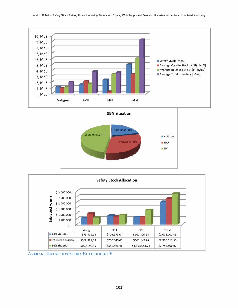
A Multi Echelon Safety Stock Setting Procedure using Simulation: Coping With Supply and Demand Uncertainties in the Animal Health Industry
103
AVERAGE TOTAL INVENTORY BIO PRODUCT Y
, MoS
1, MoS
2, MoS
3, MoS
4, MoS
5, MoS
6, MoS
7, MoS
8, MoS
9, MoS
10, MoS
Antigen FPU FPP Total
Safety Stock [MoS]Average Quality Stock (WIP) [MoS]Average Released Stock (PI) [MoS]Average Total Inventory [MoS]
$600.140,45 ; 22%
$851.666,41 ; 31%
$1.303.083,21 ; 47%
98% situation
Antigen
FPU
FPP
$ ‐
$ 500.000
$ 1.000.000
$ 1.500.000
$ 2.000.000
$ 2.500.000
$ 3.000.000
Antigen FPU FPP Total95% situation $575.005,34 $793.876,64 $662.319,68 $2.031.201,65
Intervet situation $962.821,58 $702.546,63 $663.249,78 $2.328.617,99
98% situation $600.140,45 $851.666,41 $1.303.083,21 $2.754.890,07
Safety stock volum
e
Safety Stock Allocation

A Multi Echelon Safety Stock Setting Procedure using Simulation: Coping With Supply and Demand Uncertainties in the Animal Health Industry
104
$1.438.999,57 ; 30%
$1.939.562,22 ; 41%
$1.376.556,73 ; 29%
Intervet Situation
Antigen
FPU
FPP
$1.070.344,40 ; 25%
$1.978.646,49 ; 45%
$1.329.734,21 ; 30%
95% situation
Antigen
FPU
FPP
$1.089.281,99 ; 21%
$2.080.660,71 ; 40%
$2.000.485,54 ; 39%
98% Situation
Antigen
FPU
FPP

A Multi Echelon Safety Stock Setting Procedure using Simulation: Coping With Supply and Demand Uncertainties in the Animal Health Industry
105
IMPACT OF INDIVIDUAL UNCERTAINTY FACTORS AND COMBINED UNCERTAINTY FACTORS Impact Safety Stock WIP Released Stock Total Inventory
No uncertainty $ ‐ $ 1,271,133.62 $ 1,334,760.72 $ 2,605,894.34
Demand uncertainty $ 1,144,207.80 $ 1,361,933.87 $ 1,965,059.63 $ 3,326,993.50 Lead time variability $ 975,041.47 $ 1,763,298.90 $ 1,740,618.15 $ 3,503,917.05 Yield quantity fluctuation $ 399,882.82 $ 1,392,987.14 $ 1,665,553.45 $ 3,058,540.59 Batch rejection $ 653,364.60 $ 1,402,293.22 $ 1,735,410.89 $ 3,137,704.11 Test repetition $ 494,694.42 $ 1,419,162.42 $ 1,664,014.11 $ 3,083,176.53 Yield activity fluctuation $ 506,885.78 $ 1,405,491.78 $ 1,561,349.52 $ 2,966,841.30
IMPACT OF BATCH REJECTION AND YIELF ACTIVITY FLUCTUATIONS ON INVENTORY TYPES
Sensitivity Analysis Batch Rejection
Scenario Safety Stock Quality Stock Released stock Average Total Inventory
0 * normal $ 1,767,653.28 $ 1,761,676.30 $ 2,362,075.52 $ 4,123,751.82 0.5 * normal $ 1,916,713.91 $ 1,799,405.78 $ 2,436,229.99 $ 4,235,635.77 normal rejection $ 2,031,201.65 $ 1,845,447.31 $ 2,533,277.79 $ 4,378,725.10 2 * normal $ 2,306,347.03 $ 1,918,192.94 $ 2,683,914.60 $ 4,602,107.54 Sensitivity Analysis Yield Activity Fluctuation Scenario Safety Stock Quality Stock Released stock Average Total Inventory 0 * normal $ 1,898,797.76 $ 1,822,926.54 $ 2,379,965.78 $ 4,202,892.32 0.5* normal $ 1,947,055.96 $ 1,830,128.67 $ 2,408,744.93 $ 4,238,873.60 normal fluctuation $ 2,031,201.65 $ 1,845,447.31 $ 2,533,277.79 $ 4,378,725.10 2 * normal $ 2,251,952.04 $ 1,852,019.41 $ 2,725,205.11 $ 4,577,224.52
$ ‐ $ 1.000.000 $ 2.000.000 $ 3.000.000 $ 4.000.000 $ 5.000.000
Safety Stock
Quality Stock
Released stock
Average Total Inventory
2 * normal
normal rejection
0,5 * normal
0 * normal

A Multi Echelon Safety Stock Setting Procedure using Simulation: Coping With Supply and Demand Uncertainties in the Animal Health Industry
106
IMPACT OF REDUCTIONS IN UNCERTAINTY FACTORS Optimal situation Bio product Y Antigen FPU FPP Total
Safety Stock [$] $ 575,005.34 $ 793,876.64 $ 662,319.68 $ 2,031,201.65
Average Quality Stock [$] $ 513,315.84 $ 1,173,471.78 $ 158,659.69 $ 1,845,447.31 Average Released Stock [$] $ 557,028.56 $ 805,174.71 $ 1,171,074.52 $ 2,533,277.79 Average Total Inventory [$] $ 1,070,344.40 $ 1,978,646.49 $ 1,329,734.21 $ 4,378,725.10 Optimal situation Bio product Y Antigen FPU FPP Total Safety Stock [MoS] 2.36 MoS 1.76 MoS 1.19 MoS 5.31 MoS Average Quality Stock [MoS] 2.11 MoS 2.60 MoS 0.29 MoS 4.99 MoS Average Released Stock [MoS] 2.29 MoS 1.78 MoS 2.11 MoS 6.18 MoS Average Total Inventory [MoS] 4.40 MoS 4.38 MoS 2.39 MoS 11.17 MoS Optimal situation Bio product Y Antigen FPU FPP Total Safety Stock [MoS] 1.03 MoS 1.43 MoS 1.19 MoS 3.65 MoS Average Quality Stock [MoS] 0.92 MoS 2.11 MoS 0.30 MoS 3.32 MoS Average Released Stock MoS] 1.00 MoS 1.45 MoS 2.11 MoS 4.56 MoS Average Total Inventory [MoS] 1.93 MoS 3.56 MoS 2.39 MoS 7.88 MoS
65% accuracy Antigen FPU FPP Total Safety Stock [$] $ 520,595.74 $ 754,134.87 $ 253,278.99 $ 1,528,009.59 Average Quality Stock [$] $ 512,586.62 $ 1,173,830.77 $ 160,641.44 $ 1,847,058.82 Average Released Stock [$] $ 502,871.50 $ 748,215.81 $ 766,284.22 $ 2,017,371.53 Average Total Inventory [$] $ 1,015,458.11 $ 1,922,046.58 $ 926,925.66 $ 3,864,430.36 65% accuracy Antigen FPU FPP Total
$ ‐ $ 1.000.000 $ 2.000.000 $ 3.000.000 $ 4.000.000 $ 5.000.000
Safety Stock
Quality Stock
Released stock
Average Total Inventory
2 * normal
normal fluctuation
0,5* normal
0 * normal

A Multi Echelon Safety Stock Setting Procedure using Simulation: Coping With Supply and Demand Uncertainties in the Animal Health Industry
107
Safety Stock [MoS] 2.14 MoS 1.67 MoS 0.46 MoS 4.27 MoS Average Quality Stock [MoS] 2.11 MoS 2.60 MoS 0.29 MoS 5.00 MoS Average Released Stock [MoS] 2.07 MoS 1.66 MoS 1.38 MoS 5.10 MoS Average Total Inventory [MoS] 4.17 MoS 4.26 MoS 1.67 MoS 10.10 MoS 65% accuracy Antigen FPU FPP Total Safety Stock [MoS] 0.94 MoS 1.36 MoS 0.46 MoS 2.75 MoS Average Quality Stock [MoS] 0.92 MoS 2.11 MoS 0.30 MoS 3.32 MoS Average Released Stock [MoS] 0.90 MoS 1.35 MoS 1.38 MoS 3.63 MoS Average Total Inventory [MoS] 1.83 MoS 3.46 MoS 1.67 MoS 6.95 MoS sigma leadtime 0.5 Antigen FPU FPP Total Safety Stock [$] $ 575,005.34 $ 729,953.36 $ 662,319.68 $ 1,967,278.38 Average Quality Stock [$] $ 508,125.85 $ 1,172,272.16 $ 155,104.45 $ 1,835,502.46 Average Released Stock [$] $ 566,655.55 $ 757,348.93 $ 1,116,838.95 $ 2,440,843.44 Average Total Inventory [$] $ 1,074,781.40 $ 1,929,621.09 $ 1,271,943.40 $ 4,276,345.90 sigma leadtime 0.5 Antigen FPU FPP Total Safety Stock [MoS] 2.36 MoS 1.62 MoS 1.19 MoS 5.17 MoS Average Quality Stock [MoS] 2.09 MoS 2.60 MoS 0.28 MoS 4.96 MoS Average Released Stock [MoS] 2.33 MoS 1.68 MoS 2.01 MoS 6.02 MoS Average Total Inventory [MoS] 4.42 MoS 4.27 MoS 2.29 MoS 10.98 MoS sigma leadtime 0.5 Antigen FPU FPP Total Safety Stock [MoS] 1.03 MoS 1.31 MoS 1.19 MoS 3.54 MoS Average Quality Stock [MoS] 0.91 MoS 2.11 MoS 0.30 MoS 3.30 MoS Average Released Stock [MoS] 1.02 MoS 1.36 MoS 2.01 MoS 4.39 MoS Average Total Inventory [MoS] 1.93 MoS 3.47 MoS 2.29 MoS 7.69 MoS MRP lead time Antigen FPU FPP Total Safety Stock [$] $ 483,079.10 $ 644,841.40 $ 670,822.85 $ 1,798,743.34 Average Quality Stock [$] $ 455,817.87 $ 1,117,121.29 $ 160,955.94 $ 1,733,895.09 Average Released Stock [$] $ 523,548.27 $ 708,591.39 $ 1,166,718.64 $ 2,398,858.31 Average Total Inventory [$] $ 979,366.14 $ 1,825,712.68 $ 1,327,674.58 $ 4,132,753.40 MRP lead time Antigen FPU FPP Total Safety Stock [MoS] 1.99 MoS 1.43 MoS 1.21 MoS 4.62 MoS Average Quality Stock [MoS] 1.87 MoS 2.47 MoS 0.29 MoS 4.64 MoS Average Released Stock [MoS] 2.15 MoS 1.57 MoS 2.10 MoS 5.82 MoS Average Total Inventory [MoS] 4.03 MoS 4.04 MoS 2.39 MoS 10.46 MoS

A Multi Echelon Safety Stock Setting Procedure using Simulation: Coping With Supply and Demand Uncertainties in the Animal Health Industry
108
MRP lead time Antigen FPU FPP Total Safety Stock [MoS] 0.87 MoS 1.16 MoS 1.21 MoS 3.24 MoS Average Quality Stock [MoS] 0.82 MoS 2.01 MoS 0.30 MoS 3.12 MoS Average Released Stock [MoS] 0.94 MoS 1.27 MoS 2.10 MoS 4.32 MoS Average Total Inventory [MoS] 1.76 MoS 3.28 MoS 2.39 MoS 7.43 MoS 0.5 batch rejection Antigen FPU FPP Total Safety Stock [$] $ 533,731.80 $ 799,584.59 $ 583,397.52 $ 1,916,713.91 Average Quality Stock [$] $ 498,944.80 $ 1,150,022.71 $ 150,438.26 $ 1,799,405.78 Average Released Stock [$] $ 509,598.81 $ 811,555.93 $ 1,115,075.25 $ 2,436,229.99 Average Total Inventory [$] $ 1,008,543.62 $ 1,961,578.64 $ 1,265,513.52 $ 4,235,635.77 0.5 batch rejection Antigen FPU FPP Total Safety Stock [MoS] 2.19 MoS 1.77 MoS 1.05 MoS 5.01 MoS Average Quality Stock [MoS] 2.05 MoS 2.55 MoS 0.27 MoS 4.87 MoS Average Released Stock [MoS] 2.10 MoS 1.80 MoS 2.01 MoS 5.90 MoS Average Total Inventory [MoS] 4.15 MoS 4.34 MoS 2.28 MoS 10.77 MoS 0.5 batch rejection Antigen FPU FPP Total Safety Stock [MoS] 0.96 MoS 1.44 MoS 1.05 MoS 3.45 MoS Average Quality Stock [MoS] 0.90 MoS 2.07 MoS 0.30 MoS 3.24 MoS Average Released Stock [MoS] 0.92 MoS 1.46 MoS 2.01 MoS 4.38 MoS Average Total Inventory [MoS] 1.81 MoS 3.53 MoS 2.28 MoS 7.62 MoS 0.5 yield activity fluctuation Antigen FPU FPP Total Safety Stock [$] $ 536,776.10 $ 747,960.19 $ 662,319.68 $ 1,947,055.96 Average Quality Stock [$] $ 497,313.72 $ 1,175,648.11 $ 157,166.83 $ 1,830,128.67 Average Released Stock [$] $ 497,540.85 $ 742,868.99 $ 1,168,335.08 $ 2,408,744.93 Average Total Inventory [$] $ 994,854.58 $ 1,918,517.10 $ 1,325,501.92 $ 4,238,873.60 0.5 yield activity fluctuation Antigen FPU FPP Total Safety Stock [MoS] 2.21 MoS 1.66 MoS 1.19 MoS 5.05 MoS Average Quality Stock [MoS] 2.04 MoS 2.60 MoS 0.28 MoS 4.93 MoS Average Released Stock [MoS] 2.05 MoS 1.65 MoS 2.10 MoS 5.79 MoS Average Total Inventory [MoS] 4.09 MoS 4.25 MoS 2.38 MoS 10.72 MoS 0.5 yield activity fluctuation Antigen FPU FPP Total Safety Stock [MoS] 0.97 MoS 1.35 MoS 1.19 MoS 3.50 MoS Average Quality Stock [MoS] 0.89 MoS 2.11 MoS 0.30 MoS 3.29 MoS
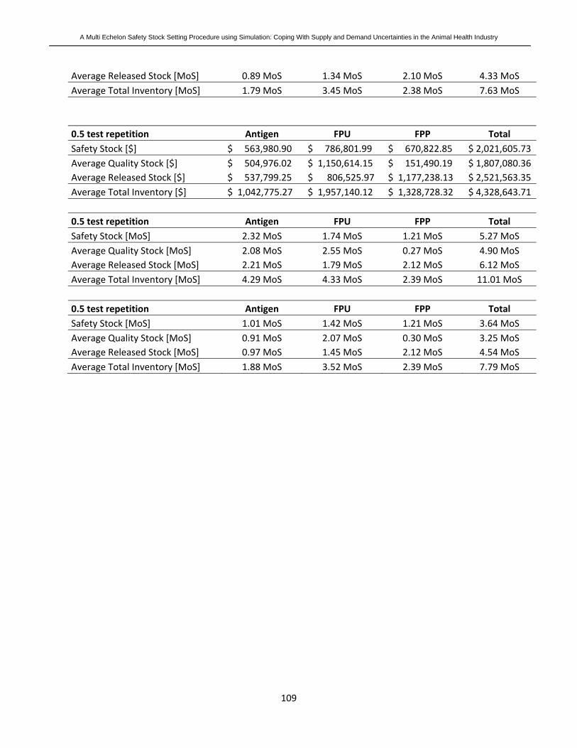
A Multi Echelon Safety Stock Setting Procedure using Simulation: Coping With Supply and Demand Uncertainties in the Animal Health Industry
109
Average Released Stock [MoS] 0.89 MoS 1.34 MoS 2.10 MoS 4.33 MoS Average Total Inventory [MoS] 1.79 MoS 3.45 MoS 2.38 MoS 7.63 MoS 0.5 test repetition Antigen FPU FPP Total Safety Stock [$] $ 563,980.90 $ 786,801.99 $ 670,822.85 $ 2,021,605.73 Average Quality Stock [$] $ 504,976.02 $ 1,150,614.15 $ 151,490.19 $ 1,807,080.36 Average Released Stock [$] $ 537,799.25 $ 806,525.97 $ 1,177,238.13 $ 2,521,563.35 Average Total Inventory [$] $ 1,042,775.27 $ 1,957,140.12 $ 1,328,728.32 $ 4,328,643.71 0.5 test repetition Antigen FPU FPP Total Safety Stock [MoS] 2.32 MoS 1.74 MoS 1.21 MoS 5.27 MoS Average Quality Stock [MoS] 2.08 MoS 2.55 MoS 0.27 MoS 4.90 MoS Average Released Stock [MoS] 2.21 MoS 1.79 MoS 2.12 MoS 6.12 MoS Average Total Inventory [MoS] 4.29 MoS 4.33 MoS 2.39 MoS 11.01 MoS 0.5 test repetition Antigen FPU FPP Total Safety Stock [MoS] 1.01 MoS 1.42 MoS 1.21 MoS 3.64 MoS Average Quality Stock [MoS] 0.91 MoS 2.07 MoS 0.30 MoS 3.25 MoS Average Released Stock [MoS] 0.97 MoS 1.45 MoS 2.12 MoS 4.54 MoS Average Total Inventory [MoS] 1.88 MoS 3.52 MoS 2.39 MoS 7.79 MoS