Embed Size (px)
Citation preview

Eindhoven University of Technology
MASTER
Determination of the impulse response of a mobile channel by simulation : a deterministicapproach
van der Hulst, René
Award date:1987
Link to publication
DisclaimerThis document contains a student thesis (bachelor's or master's), as authored by a student at Eindhoven University of Technology. Studenttheses are made available in the TU/e repository upon obtaining the required degree. The grade received is not published on the documentas presented in the repository. The required complexity or quality of research of student theses may vary by program, and the requiredminimum study period may vary in duration.
General rightsCopyright and moral rights for the publications made accessible in the public portal are retained by the authors and/or other copyright ownersand it is a condition of accessing publications that users recognise and abide by the legal requirements associated with these rights.
• Users may download and print one copy of any publication from the public portal for the purpose of private study or research. • You may not further distribute the material or use it for any profit-making activity or commercial gain

Faculty of Electrical Engineering Eindhoven University of Technology Telecommunications Division EC
Determination of the Impulse Response
of a Mobile Channel by Simulation.
A deterministic approach.
René van der Hulst.
Thesis on a study of propagation effects in mobile communications, performed at Dr. Neher Laboratories in L~idschendam during the period from March 1986 until February 1987.
Professor: Coaches:
Prof. Dr. J.C. Arnbak Ir. W. van Blitterswijk (DNL) Ir. W. van Eek (DNL) Ir. P.M.J. Scheeren (EUT)
The faculty of Electrical Technology disclaims all graduation reports.
Engineering of the Eindhoven University of responsibility for the contents of training and

SUMHARY
Characteristic for the mobile radio channel is the movement of a mobile station in a multipath environment, which results in a time varying impulse response. For the planning of wideband mobile radio systems it would be of great help to be able to predict impulse responses from the characteristics of the mobile station's environment.
The objectives of the study subject of this thesis were to verify whether or not the mobile channel could be described by a relatively simple model, to obtain insight in the influence of the Doppler shift on the variability of the impulse response, and to develop simulation software. Purpose of the simulation is to get an impression of the variability of parameters in typical situations; not to obtain a deterministic prediction for all situations.
The thesis treats the mathematica! representation of the mobile multipath channel and discusses several models for the scattering by buildings. Initially, no attention was given to the question whether scattering was coherent or incoherent. In the end of the study, this aspect appeared to give additional information about the validity of the models for scattering from buildings.
The simulation model described in this thesis is developed assuming coherent scattering. The basic idea is to assign a scatter diagram to each relevant building and to determine in a deterministic way, which propagation paths are possible between transmitter and receiver. To be able to describe the behaviour of a scattering surface by an expression for the far field, this surface is divided into effective scattering elements if the mobile is in the near field. With this model, the influence of the Doppler shift on the phase shift and the shift in time delay associated with a displacement of the mobile can be determined. For incoherent scattering however, the influence of the Doppler shift may be canceled by a shift in phase and time due to the roughness of the scattering surface.
The study has many open ends and some suggestions are done for further research. In particular it is recommended that the data obtained by wideband measurementsis analyzed tapwise, i.e. that the characteristics of the signa! level at the same relative time delay in subsequent impulse responses are determined. From this information, more insight might be obtained about the coherence or incoherence of the mobile channel.

CONTENTS
1. Introduetion 2
1.1. 1.2. 1. 3. 1. 3.
General Radio subsystem design ............................................. . Contiguration of the mobile station ................................ . System performance simula ti on ...................................... .
2 3 5 5
2. Propagation between base station and mobile station ...................... 7
2. 1. General . . . . . . . . . . . . . . . . . . . . . . . . . . . . . . . . . . . . . . . . . . . . . . . . . . . . . . . . . . . . . 7 2.2. Narrowband characteristics .......................................... 7 2.3. \olideband characteristics ............................................ 9
3. Modelling mobile channel's propagation characteristics ................... 11
3.1. Purpose of rnadelling ................................................ 11 3.2. Strategy ............................................................ 11 3. 3. Restrictions ........................................................ 12 3. 4. Subdi vision of the model . . . . . . . . . . . . . . . . . . . . . . . . . . . . . . . . . . . . . . . . . . . . 12
4. Mathematica! model for the mobile channel ................................ 14
4.1. The relevant physical parameters .................................... 14 4.2. The impulse response of the channel ................................. 15 4.3. Characterization of the mobile channel ..........................•... 18
5. The influence of scattering objects ...................................... 19
5.1. First model for scattering .......................................... 19 5.2. Definition of terms associated with scattering ................•..... 22
5.2.1. Coherence and incaherenee of the scattered field ............. 22 5.2.2. Distietion between distant and nearby scatterers ............. 23 5.2.3 Definition of the scatter coefficient ........................ 24
5.3. Scattering from buildings according to Bramley and Cherry ........... 25 5.4. Scattering from rough surfaces according to Lambert ................. 25 5.5. Scattering by smooth and rough surfaces .................•........... 25
5.5.1. Introduetion ................................................. 25 5.5.2. Determination of the scatter coefficient ..................... 26
6. Simula t ion . . . . . . . . . . . . . . . . . . . . . . . . . . . . . . . . . . . . . . . . . . . . . . . . . . . . . . . . . . . . . . . 32
6.1. Introduetion ........................................................ 32 6.2. Channel simulation .................................................. 32
6.2.1. Creation of a database ....................................... 32 6.2.2. Division into effective scattering elements .................. 33 6.2.3. Determination of valid propagation paths ..................... 33 6.2.4. Calculation of the distribution functions .................... 35
6.3. Filter simulation ................................................... 38 6.3.1. Pulse shape and spectrum ..................................... 38 6.3.2. Filter spectrum .............................................. 39
7. Verification ............................................................. 41
7.1. Determination of the scatter diagram of buildings by measurement .... 41 7.1.1. The measurement setup ........................................ 41 7 .1. 2. Re sul ts . . . . . . . . . . . . . . . . . . . . . . . . . . . . . . . . . . . . . . . . . . . . . . . . . . . . . . 42
7.2. Verification of the simulation software ...........•................. 43 7.2.1. Simulation of a fictive situation ....................•......• 43 7.2.2. Simulation of a real situation ............................... 48
8. Conclusions and Recommendations .......................................... 50
9. Liter a ture . . . . . . . . . . . . . . . . . . . . . . . . . . . . . . . . . . . . . . . . . . . . . . . . . . . . . . . . . . . . . . . 52
Appendix . . . . . . . . . . . . . . . . . . . . . . . . . . . . . . . . . . . . . . . . . . . . . . . . . . . . . . . . . . . . . . . . . . . . 54
A. Scattering from rough surfaces .................................•......... 54 A.1. General salution .................................................... 54 A.2. Rough surfaces as random process .............................•...... 63 A. 3. Resul ts and discussion .............................................. 72

Page 2
1. INTRODUCTION
1.1. General
In Europe, the use of public landmobile communication systems is expanding rapidly and it is to be expected that soon the capacity of existing systems will be insufficient. Therefore there is a need to develop new systems with a larger capacity.
In order to specify a common system for landmobile communications in the 900 MHz band, which is to be operated in at least all CEPT~countries, the CEPT established the GSM (Groupe Sp~cial Mobile). One of the tasks of GSM is to compare the possible types of radio sub systems [1]. This comparison comprises three stages:
1. elimination of those systems which do not meet minimum requirements with respect to:
- the transmission channel quality; the peak traffic density;
- the size, weight and power consumption of hand-held stations; - the bandwidth, which may not exceed a maximum; - the costs of the system, which shall not be bigger than that
of any well established analogue public system;
2. comparison of the remaining systems with respect to costs and spectrum utilization;
3. finally, if more than one system remains, selection of the system which offers most flexibility in frequency planning and system engineering and which makes it possible to follow the technica! evolution (lower speech bit rates).
In principle, it bas not been decided yet whether the new system will be analogue or digital. However it bas become clear, due to the availability within Europe of a number of analogue systems in the 900 MHz band that, if the choice will not be in favour of a digital system, there will be no European system. Therefore GSM concentrates its efforts on the research on and the comparison of digital alternatives. The final choice between the analogue and digital options will be made in the beginning of 1987, when the results of experiments with the digital alternatives will be available. The choice will be determined also by the necessity to have an operational system before the end of 1991, for if this deadline is not met, the 900 MHz band will be fully occupied by what CEPT calls 'interim' systems.
The scope of this thesis will mainly be on digital systems, since the study which is the subject of this thesis bas been done in the context of the work of GSM.
CEPT*= Conf~rence Européenne des Administrations des Postes et T~lécommunications.

1.2. Radio subsystem design
The design of the radio subsystem in a communications is an optimization problem. between alternatives for:
- the bitrate; - the channel coding; - the modulation technique; - the multiple access scenario; - the frequency reuse factor; - the transmitted power.
Page 3
digital system for mobile Choices will have to be made
Design criteria for the system are that the system shall meet minimum requirements on transmission channel quality and system capacity. Most important criteria for the final choice are spectrum efficiency and cost.
In the most basic form, the radio subsystem consists of three elements, as illustrated in figure 1. The radio channel is the most typical part in a system for mobile communications, for it allows the mobile station to move around freely.
base _L_ mobile _L mobile
tranceiver channel tranceiver
unit I I
unit
Figure 1 Elements of the radio subsystem.
To be able to communicate over this channel we need a transceiver located in a fixed or base station at one side and a transcelver in the mobile station at the other side.
Often the total number of radio channels available to a mobile radio system will not provide sufficient capacity to cover a large area. The capacity can be increased by spatial reuse of the radio channels, which is a form of spatial multiplexing. This accounts for the cellular structure of most mobile radio systems. The cells operating the same frequencies, shall be sufficiently separated to prevent excessive co-channel interference. This separation is assured by cell clustering where each channel is allowed to appear in the cluster only once. An illustration of cellular coverage with examples of different cluster sizes is given in figure 2.

Figure 2
SPEECH DECODER
Figure 3
Example of some hexagon clusters of different size.
-~
SPREAOER :
- .J
r-1 DESPREADER I I L ___ .J
HOOULATOR
MULTIPLE
POWER AMPLIFIER
FRONT END RECEIVER
Contiguration of the mobile station.
Page 4

Page 5
1.3. Contiguration of the mobile station
The mobile station consists of a transcelver unit and a speech (de)coder. This (de)coder is the interface between the digital transmission system and the analogue world. The contiguration of the mobile station is illustrated in figure 3. The tunetion of the elements of the station will be described briefly.
The purpose of the speech coder is to convert the analogue speech signa! into a digital signa! with a limited bitrate. The existing technology allows for a 16 kbit/s bitrate, but new technology could bring the minimum rate down to 8 kbit/s, thus doubling the system's capacity.
The channel coder adds redundant information to the speech cocled signa! in order to enable error detection and correction after transmission.
Some systems offer the possibility of implementing a spread spectrum technique. Spread spectrum techniques might be used to make the signa! less sensitive to randomly located bit errors, caused by a low signal-to-noise ratio.
To enable the transmission of the digital signa! over the analogue transmission channel, it is necessary to embed the baseband signa! in a carrier waveform by digital modulation. For application in mobile communications, constant envelope modulation techniques are most suitable.
In order to allow access to the transmission channel by more than one user at a time, a multiple access controller decides in what channel the mobile may transmit or will receive data. The channel allocation will be clone by the base stations using a dedicated control channel.
1.4. System Performance Simulation
A final system concept shall be evaluated with respect to the set of requirements. In principle there are three methods of evaluation:
- a software simulation of both system and propagation characteristics to determine the system's performance;
- measurement of the performance of a system prototype in a laboratory environment using a hardware channel simulator;
- field measurement of the performance of a system prototype.
For both software simulation and simulation using a hardware channel simulator, it is important to develop a realistic model of the mobile channel's propagation characteristics. The development and verification of such a model are the main subjects of this thesis.
After a global introduetion to the influence of propagation characteristics on narrowband and wideband systems and a discussion of the purpose and restrictions of the model to be developed, a mathematica! model is introduced which gives the parameters that are relevant for the characterization of the mobile channel. Next, scattering by buildings is discussed. In the course of the study on propagation mechanisms, the

Page 6
importance of this subject became clear.
Initially, the study concentrated only on the mean scattered power, trying to assign a scatter diagram to each building. Instead of a fundamental study, intuition was followed in an attempt to define a scatter diagram. However, the verification of the results by measurement became impossible, due to interterenee by a radar signal. This focused the attention on a theoretical study of scattering from buildings. Several approaches are discussed in this thesis. Still, an important aspect was underrated. The influence of the scattering by buildings on the phase of the received signal is a determinating factor. Thus, the attention given to this subject is not in proportion to the apparant importance of the subject.
The simulation software as described in this thesis, implements the mathematica! model of the mobile channel. The purpose of the software is to get an impression of the variability of parameters in typical situations, not to obtain a deterministic predietien for all situations. Some remarks are made on the results of the simulation using this software and possible ways of verification are indicated. Finally, the results of the study are discussed and some recommendations are made for future research.
Page 7
2. PROPAGATION BETYEEN A BASE STATION AND A MOBILE STATION
2.1. General
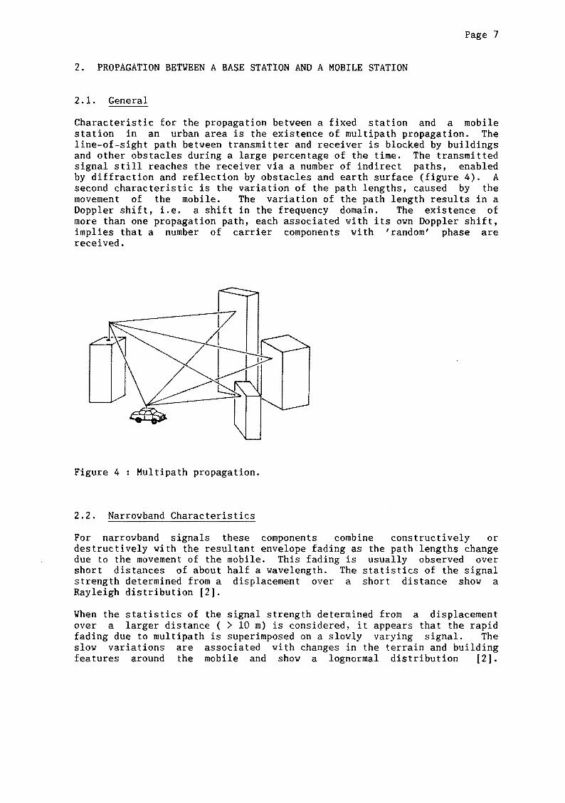
Characteristic for the propagation between a fixed station and a mobile station in an urban area is the existence of multipath propagation. The line-of-sight path between transmitter and receiver is blocked by buildings and other obstacles duringa large percentage of the time. The transmitted signal still reaches the receiver via a number of indirect paths, enabled by diffraction and reflection by obstacles and earth surface (figure 4). A second characteristic is the variation of the path lengths, caused by the movement of the mobile. The variation of the path length results in a Doppler shift, i.e. a shift in the frequency domain. The existence of more than one propagation path, each associated with its own Doppler shift, implies that a number of carrier components with 'random' phase are received.
Figure 4 Multipath propagation.
2.2. Narrowband Characteristics
For narrowband signals these components combine constructively or destructively with the resultant envelope fading as the path lengths change due to the movement of the mobile. This fading is usually observed over short distances of about half a wavelength. The statistics of the signal strength determined from a displacement over a short distance show a Rayleigh distribution [2].
Yhen the statistics of the signal strength determined from a displacement over a larger distance ( > 10 m) is considered, it appears that the rapid fading due to multipath is superimposed on a slowly varying signa!. The slow variations are associated with changes in the terrain and building features around the mobile and show a lognormal distribution [2].

Page 8
Furthermore, the signal strength decreases with increasing distance between mobile and base station. The relation is exponential, with an exponent between 1.75 and 2.0 [2]. Thus the received signal strength 1~1 can be expressed as:
IE I = A(r) * B(building/terrain features)* C(x,y,f) * IE 1, -r -o
with:
A = attenuation coefficient due to distance ( A 1.75 <a< 2.0;
-a (r/r0
) ) ,
B
c
coefficient depending on the overall building and terrain features around the mobile. This coefficient has a lognormal distribution; coefficient depending on the frequency and the rnabile's position. This coefficient has a Rayleigh distribution; signal strength at a distance r
0 from the transmitter.
An example of a mobile received narrowband signal is given in figure 5.
G> '0
2 Q.
E OCD
- '0 :?....: .2'~ ~~
"' >
0 Q)
0:::
Left·side scole
0
R!Qhl side scole
----Averoge received power P(Jt~ c: --Received siQnol in termsof "...,.. 8 .g
distonce x, s (x) . ..-· .2 .-·-- 7 ~
--·- G> ~· ~ • 0
6.0~ E . !?"U
Distance travelled
5-0 Q) c o-C: c:!! 0 c O::o
(1)
Figure 5 Variation of the fieldstrength with the rnabile's position [2].
Different models have been developed to predict the average propagation loss (A2 .B 2 ). An empirica! methad for power loss prediction has been provided by Okumura [3]. This methad relates the loss at any place to the loss at a position in an urban area over 'quasi smooth' terrain and with a reference transmitter and receiver antenna height. Okumura produced eight factors in graphical representation, to correct for suburban and open areas, terrain features, antenna heights etc .. The methad is often quoted since it is almast the only technique readily available that is specifically intended to be used for built-up areas and which takes into account variations in terrain and urbanization. Based on Okumura's method, Hatta [4] derived a formula to allow the methad to be implemented on a computer. The main objection to Okumura's methad is that his model is based on measurements performed in the USA and that for application elsewhere new curves and new classes should be defined to represent the 'local' situation.

Page 9
2.3. ~ideband Characteristics
In the case of wideband signals and a wideband receiver, the different propagation paths might be distinguished in the impulse response of the mobile channel (figure 6). A difference in path length results in a difference in time delay, which can be observed if the bandwidth of the receiver offers sufficient resolution in the time domain.
~SO
..... • = -40 ~ ... .. .<o " 0 ...
~6o
-jo
-8c
-~0
0
Figure 6
1 ft 8 10
Time delay (l's)
Impulse response of the mobile channel with a wideband receiver [5].
For example, if we consider two propagation paths with a difference in path length of 300 m, the difference in time delay will be about 1 ps. Thus, using a receiver with a bandwidth B larger than 0.5 MHz - corresponding to a resolution in the time domain of at least 1/28 = 1 ps the two paths can be distinguished in the impulse response. For a bandwidth less than 0.5 MHz the pulses received over the two propagation paths interfere, which results in a fading envelope.
From this example, it may be clear that a distinguishable peak in the impulse response correspond to a cluster of scattering objects. This means that the fading on one peak is independent of fading on other peaks in the impulse response. So, if the receiver employs the signal power from a number of these independent fading peaks, it should be able to regain the information from the received signal during a great percentage of time. This is the potentlal advantage of wideband systems over narrowband systems.
However, due to the rnabile's movement, the path lengths, being position dependent, change. The result is a shift in the time domain causing the impulse response to be position dependent (note the analogy with the

Page 10
Doppler shift when consirlering the response to a frequency impulse of a narrowband system). Therefore, since the receiver has to know the channel's impulse response to be able to regain the transmitted signal, it should determine this impulse response regularly.
For the planning of wideband systems for mobile communication it would be of great help to be able to predict impulse responses and their variability from environmental characteristics.

Page 11
3. MODELLING THE MOBILE CHANNEL PROPAGATION CHARACTERISTICS
3.1. Purpose of modelling
Characteristic for propagation over a mobile transmission channel is that
- the time delays differ for successive propagation paths; - due to the mobile's movement, the length of the propagation
paths is time-dependent.
The time-dependency of the propagation path length results in fading and shifting of peaks in the impulse response.
The purpose of developing a model, from which the characteristics of the mobile channel can be calculated, is to
- determine whether the mobile channel can be simulated usefully from characteristics of the mobile's environment by a relatively simple model;
- obtain insight into the consequences of the Doppier shift for the impulse response of the mobile transmission channel;
- enable a software simulation of the transmission channel, which will be used to determine the consequences of the Doppier shift for the performance of various modulation techniques.
3.2. Strategy
Most simulations of the mobile channel propagation characteristics are based on a statistica! approach [2,5,6]. The statistica! approach is appropriate to the systems with narrowband signals, because the various propagation paths cannot be distinguished in the time domain. Rapid variations of the signa! strength due to multipath fading can be compensated by relatively simple solutions, e.g. antenna diversity [2,7].
Videband signals and receivers however require a different approach. Most wideband receivers for mobile communication systems determine the impulse response of the mobile channel at the beginning of a transmission time slot. During the rest of the time slot, the system assumes the impulse response to be time independent. To verify this assumption or, differently stated, to determine for which length of the time slot this assumption is correct, it is important to determine the variations of the impulse response during the displacement over some wavelengths. A statistica! approach would average the variations, thus wasting the required information. Therefore in modelling the propagation characteristics for mobile wideband communication systems, a deterministic approach will be followed.

Page 12
3.3. Restrictions
The simulation of the mobile channel's propagation characteristics should be as realistic as possible. However, it is evident that an exact and complete simulation of the reality is impossible. An attempt to approach a complete simulation would imply a very complex model, which is not likely to increase the understanding of the relevant mechanisms of propagation in an urban area; for that reason such a model is undesired. Therefore a number of restrictions are introduced here.
- Only the mobile is supposed to be moving, scattering objects are assumed to be fixed. This restrietion eliminates the changes in the impulse response which would be present even if the mobile station was not moving.
Ground reflections are neglected, for they would require an additional multipath analysis with respect to the height. This is an undesired complication. Consequence of this restrietion is that additional fading which might be caused by interterenee of the ground reflection and the signal received over the direct path is eliminated.
- Diffraction is neglected. As concluded by Van Rees [8] multipath is an effect far more important.
- The mobile moves with constant speed along a straight line. Actually this is not a restriction, for this condition will always be met if the interval over which the mobile moves is taken small enough.
- Depolarization effects of the mobile channel on the transmitted radio signal will not be considered. Yhere it is necessary to assume a polarization of the radio signal, vertical polarization will be used. In mobile communications this is the usual polarization, since the antenna on top of the mobile is supposed to be omnidirectional in the horizontal plane. The power measured in a real situation will therefore be less than the power calculated in the simulation.
3.4. Subdivision of the model
The development of a model for the mobile channel can be made more systematically if the problem is divided into well defined sub-problems. Realizing that the model of the mobile channel should provide a clear physical insight into the propagation mechanism, but should also provide system related parameters, the following sub-problems can be distinguished (figure 7) :
- a model for the scattering from buildings is needed to find realistic values for the scattered power; the problem is to find such a model;

Abstract representation of the mobile' s environment
Mathematica! model of the channel characteristics
Model of the scatter behaviour of buildings
Model of the mobile channel
Figure 7 Modules of the model.
the environment shall be represented in an stylized way, because it is not possible to represent every detail. Therefore the characteristic aspects of objects in the environment have to be determined;
- to be able to obtain parameters which are relevant for communication systems, a mathematica! model is neerled to characterize the mobile channel.
These sub-problems will be discussed in the next chapters.
Page 13

Page 14
4. MATHEMATICAL MODEL OF THE MOBILE CHANNEL
4.1 . The relevant physical parameters
As discussed in chapter 2, propagation paths having approximately the same time of arrival may be related to clusters of scattering objects. However, it is not possible to distinguish between different paths merely by considering the difference between the times of arrival. The angular direction of arrival also has to be taken into account. If on each path the signal is scattered once and only once, all scatterers associated with the same time delay are located on an ellipse with the receiver and the transmitter at its loci (figure 8).
, "' ,
Figure 8
B
\ d;r~ct ion
of mo1ion
Relation between position and time delay for single scattering (9) .
It is possible to distinguish between the paths 1 and 2 by their different angles of arrival at the mobile station, i.e . the spatial angle between the direction in which the scatterer is seen from the mobile point of view and the direction of motion of the mobile (figure 9).
'Whenever a shift observed station radiated relative
the station is in motion, each angle of arrival is associated with in the frequency domain - i.e. a Doppler shift -, which might be
from the spectrum of the received signal. Consider a mobile which moves at a speed v. An elementary wave received by, or from an antenna on top of that station has a phase velocity to the station given by:
v f = c - v. cos a . (2)
Therefore the frequency observed by the receiver is equal to
f v - - · . cos a . (3) A

Page 15
, //\"-
-- __ ,..-----./----.,_ ------
incoming /wov~
do-f'clion of motion
Figure 9 Angle of arrival [9].
Hence, the Doppler shift is defined as:
4.2. The impulse response of the channel
To be able to use the lowpass equivalent representation of signals and filters [10],
(4)
the input signal of the channel has to be centred in the frequency domain around the carrier frequency fc. Therefore, an RF pulse (figure 10) is defined by:
x(t) = a(t).cos(wct) , (5)
where a(t) is symmetrical around t=O and has unit area. The impulse response is the response of the lowpass equivalent channel to a(t). The duration of a(t) is assumed to be very short compared to the response time of the filters used.
Figure 10 RF pulse.
If this signal has suffered multipath propagation, it constitutes a set of attenuated delayed and phase shifted replicas of the transmitted RF signal. The resultant signal received is a superposition of contributions from the various individual paths. Since the path lengths change if the mobile moves, the channel's response to (5) is position dependent. In order to be

Page 16
able to discriminate between different effects which determine the phase of the received signal, the path length p· is defined as the length of the propagation path if all scattering surfaces would be perfectly smooth. The deviation from this path length due to the rougness of a surface is represented by si. So the received signal y(t,r) can be written as:
where
E c.a(t-T.).cos{2~f (t-T.)J, i 1 1 c 1
is the attenuation over propagation path i; is the time delay associated with path i, given by T. (r) = {p,(r)+s,(r)}/c
1 - 1 - 1 ~
(6)
If the mobile station moves, the frequency of the signal component arriving over path i experiences a Doppler shift fd., so that
1
E c.a(t-T.).cos{2~(fc+fd,)(t-T1·)J i 1 1 1 (7)
or, in low pass equivalent notation [10]:
(8)
Since a(t) is very short compared to the response time of the filters used, in the low pass representation a(t) has the same properties as the dirac function. Hence:
-jw T· yLP(t,r) = 2: c.a(t-T.).e c 1 • (9) i 1 1
To get an impression what consequences the position dependency of the channel transfer has, the response is considered at position r+ör. Por small lörl, the path length p(r+ör) is given by
P(!') + löEI·cosa. ( 10)

Page 17
Thus, the phase shift resulting from the change in path length, due to the displacement, is given by
ó~p= P(E+óE)-p(E) .2~
À
JórJ v = __ -_ ._. fc cosa.. 27T V C
= lóE I . fd . 2rr. V
The phase shift resulting from a change in s is given by
ós
À • 27T.
In analogy with (11) and (12) the shift in time delay is given by
ÓT = P(E+óE)-p(r) p c
!M:! td =-·-V fc
and
ÓT 5 óS• = _1.
c
(11)
(12)
(13)
(14)
These results will be discussed briefly here. From (12) it appears that if lós I <<À, the phase shift due to the roughness of the scattering surface is negligible and the phase shift caused by the displacement can be described by the spatial frequency, i.e. the ratio of the Doppier shift and the velocity of the mobile station. However, if lós I > À, the signal looses all phase information and the phase shift will be random.
The total shift in time delay is the sum of ÓTP and 6T 5 :
ÓT = ÓTp + 6T 5 • (15)
On the total shift a simular discussion as the above can be given. The maximum shift in the time delay domain can be calculated if the maximum value of lós I is given:
ÓT max JÓ!: cosa.! + Jósl
c c (16)

Page 18
Note that if the Doppler shift is to be determined from the time delay or phase measured using a station moving at constant speed v, the ratio T = ~~~1/v is the sample interval in the time domain. 8
4.3. Characterization of the mobile channel
From the previous section it appears that four parameters describe each path of the mobile channel:
- attenuation; - time delay; - Doppler shift; - phase shift.
Therefore the mobile channel is completely determined by the distribution of the in-phase and quadrature component of the field over the time delay and the Doppler shift.
Since it is assumed that the duration of x(t) and thus a(t) is very short compared to the response time of the filters used, sampling of the impulse response given by (9) is not realistic; most pulses would be lost in the process of sampling. Therefore, in the ultimate model, the time delays and the Doppier shifts are quantized, which corresponds to the representation of the channel by a densely tapped delay-line transversal filter [11].
Figure 11 Tapped delay-line model of the mobile channel.

Page 19
5. THE INFLUENCE OF SCATTERING OBJECTS
5.1. First model for scattering
A lot of research has been done on reflection and diffraction by the surface of the earth, but little is known about scattering from buildings and other obstacles, especially in the frequency band of interest (900 MHz).
At frequencies about 900 MHz, measurements were performed by Van Rees [12] and by Ikegami and Yoshida [13]. Van Rees concluded that the effect of buildings and obstacles can be described by the radar equation, using the Lambertian diffuse scattering model. For local scatterers however, a radar cross section was found which appeared to be significantly lower than that of distant reflectors (-20 dB).
Ikegami and Yoshida explained their observations using Snellius reflection, knife edge diffraction and tunneling, and concluded that the effect of objects nearby can be described by ray tracing techniques.
Based on the conclusions of Van Rees [12] and of Ikegami and Yoshida [13] the following model for the scatter behaviour of buildings and other objects was adopted.
Objects nearby were assumed to be mirrors reflecting only in the direction, i.e. the direction according to Snell's reflection average power loss per reflection was supposed to be 6 dB, as (though not motivated) by Ikegami and Yoshida [13].
specular law. The suggested
Distant objects, on the contrary, were radiation according to Lamhert's law, incidence and polarization, the scattered angle82 to the normal to the surface, is
considered to scatter incident so that, for any direction of
power per unit solid angle, at an proportional to cose2.
Then the radar cross section of these distant objects can be expressed as:
~ = 4A. cos(e ).cos(e ), 1 2
(17)
with: ~ = the radar cross section; A the area of the scattering surface; el angle of incidence; 82 angle of observation.
The scatter behaviour of buildings and other objects as discussed above was implemented in an stylized model of the physical situation, from which time delays, Doppier shifts and the power of the signals received over the successive paths could be calculated (figure 12). In the model, the order of multiple reflections was limited to three. Restrictions were imposed with respect to the position and orientation of the second and third reflector; they were supposed to be nearby and parallel to the mobile's direction of movement. These restrictions were regarded as quite realistic and allowed a simple mathematical analysis. Shadowing was not taken into account.

Page 20
I .i/IJUIAI4 I ,~
I I I I I I
: L\ I illJJII r----- ---;;..-ïiii#iï-- ----------- ----~
i """' r ~~
~ i BASE STATION
Figure 12 Stylized model of a physical situation.
Using the particular mathematica! model of the wideband transmission channel described in chapter 4, the impulse response of the channel was calculated. From the results, it appeared that the simplified model of the physical situation was inadequate. Main objection to this model is that it produces too few propagation paths to provide a realistic impulse response, even if shadowing is not taken into account. This is illustrated by a presentation of the impulse response obtained from field measurements (figure 13) and the impulse response calculated by simulation, using the stylized representation of the mobile's environment (figure 14).
The two impulse responses may be compared, since the bandwidth of the filter used in the simulation is about the same as the bandwidth of the receiver filter used with the measurements (i.e., approximately 20 MHz).
As can be seen from figures 13 and 14, the shape of the measured impulse response is more irregular and shows more response at larger time delays (>3 ps). Furthermore, comparison of impulse responses calculated for successive positions of the mobile, shows that the variation of the signal strength at a fixed time delay is much less than the changes in signal level at fixed time delays in the measured impulse response (at a bandwidth of 20 MHz).
The most likely explanation is that the number of propagation paths found by the simulation is not large enough. Possible causes are that:
- the model of the influence of scattering objects is inadequate;
- the limit on the order of multiple scattering is unrealistic;
- the number of reflectors cq. scattterers included in the stylized representation of the mobile's environment is not large enough.

Page 21
-30
" "' - l.jo -o
... " _ço :> 0
0..
-~
-jo
-Jo
_,,o u
0 8 10
Time delay (fiS)
Figure 13 Impulse response obtained by field measurement [14].
0
~
"' -o
... -10 " :. 0 0.
"' >
:;; - -20 ., ""
0 3 9 !2 l 5
Figure 14 Impulse response calculated by simulation.

Page 22
Therefore it was decided to develop a new model, taking into account the experiences with the first model.
5.2. Definition of terms associated with scattering
5.2.1. Goherenee and Incoherence of the scattered field
If the phase of a of length 2n, the is constant it is incoherence of consideration in illustration.
wave is random and uniformly distributed over an interval wave will be called incoherent. If the phase of the wave a coherent wave. Beckmann [15] treats the coherence and the scattered field on the basis of a geometrical
two dimensions, which will be given here as an
2
2
Figure 15 Geometrie illustration. [15]
Consider two elementary waves scattered by a rough surface with a length X >>À. The height of the irregularities is limited by Zmax <<X. The phase difference between the two waves scattered at the points Z(xi) and Z(x
2) of
the surface (figure 15) is given by
where: ·- k -1
!l is the propagation vector of the incident field, given by = 2rr.(sine
1e -cose e ); T -x 1-z
is the propagation vector of the scattered field, given by 2rr. (sine e +cose e ) ; À. 2 -x 2 -z
x. e + Z(x )e ; l -x 1 -z
x_ e + Z(x2
)e • -"Z -x -z

Page 23
Thus 6~ is given by
(19)
Since Zmax <<X and (x1 -x2 )max =X, the first term in (19) will be dominant for the non-specular· direction and the phases of the elementary waves scattered in the direction 82 will vary in the interval
(20)
For 8 1 ~ 82 , 6~ might vary over many intervals 2TI. Hence the phases of the individual scattered waves are in effect uniformly distributed over an interval of length 2n. Beckmann [15} concluded that outside a narrow cone about the specular direction, the amplitude of the field scattered by a rough surface is always Rayleigh distributed. If the surface is very rough and grazing incidence is excluded, the amplitude of the scattered waves is Rayleigh distributed everywhere.
5.2.2. Distinction between distant and nearby scatterers
Usually, the approach for the calculation of the surface is based on the assumption that at the scattered wave is plane rather than spherical. Fraunhofer zone of diffraction.
field scattered by a point of observation the This is true for the
According to Rayleigh's far field criterion [16}, the transition to the Fraunhofer zone for a point observer occurs about a distance
(21)
from a circular aperture with diameter D. For a rectangular aperture, D should be substituted by the lengthof the rectangle's diagonal. Thus for a rectangular aperture of length 1 and height h, the transition to the Fraunhofer zone occurs about a distance
(22)
Using (22), a scatterer is defined to be distant from a mobile station if the distance to the station is larger than Rf. If not, the scattereris defined to be nearby.
To be able to use an expression for the scattered field in the Fraunhofer zone of diffraction for nearby scatterers, the nearby scatterer is divided into elements with smaller dimensions, until these elements satisfy (22). Thus, the near field of the complete surface becomes the superposition of the far fields of the surface elements (figure 16).

to point of observation
far field near field
Figure 16 Near field and far field approach [15].
5.2.3. Definition of the scattercoefficient
Page 24
The quantity which describes the scattering from the surface of an object is the scatter coefficient Sc. Sc is defined as the ratio of the flux S~ of the scattered field in a point P at a distance Ro from the scatterer and the flux S1 of the incident field at the surface of the scatterer (figure 17).
Tx
Rx s~
Figure 17 Definition of the scatter coefficient.

Page 25
5.3. Scattering from buildings according to Bramley and Cherry
Bramley and Cherry [17] investigated scattering by tall buildings at 9 GHz and concluded that for this frequency - with a wave length of about 3 cm -scattering characteristics can be explained reasonably well in terms of scattering from a large number of smooth flat elements, which correspond to visible features of buildings. They suggested that the result may be used to estimate the scattering at other frequencies of interest, for they showed that the frequency dependenee of the dielectric properties of building materials are unlikely to be important. However, they pointed out that it is rather complicated todetermine the dominant geometrical factors and stressed the necessity to consider these factors in detail for each particular frequency.
5.4. Scattering from rough surfaces according to Lambert
In genera!, the surface of a building is not a homogeneous, smooth structure, but consists of a large number of elements like concrete slabs, windows, window-frames, balconies, etcetera. As mentioned before, the scatter diagram of such a surface may be considered to be a composition of the scatter diagrams of smooth elements corresponding to the visible features. However, if the dimensions of these features are in the same order of magnitude as the wavelength, it seems more appropriate to consider such a surface as being rough.
As be is
Sc
mentioned modelled
given by:
A.cose
insection 5.1., the scattering from ideal rough surfaces can by Lamhert's law (17). In that case, the scatter coefficient
(23)
The shape of the scatter diagram, given in figure (18) is independent of the angle of incidence.
This model is confirmed by the measurements performed by Van Rees [12]. If according to section 5.2.1. - a nearby scatterer is divided into elements
small enough that each element is distant to the mobile station, the effective scattering area becomes smaller which might explain the difference which Van Rees found between the radar cross section measured for local scatterers and the radar cross section according to (17).
According to section 5.2.3., the field scattered by a very rough surface is incoherent, which implies that the phase is a random variable, uniformly distributed over an interval with length 2rr.
5.5. Scattering by smooth and rough surfaces
5.5.1. Introduetion
The ideal mirror and the ideal scatterer are extremes among the models for the scattering from smooth, respectively rough surfaces. Here, some attention will be given to a model which includes smooth, moderately rough and very rough surfaces.

ro !O ~
~ 0 c V ~ u -10 ~ ~ ~
-~0 ~ 0 0 _, ~ ID ~
.8o ~ ~ u ~
-jO _,
-30 0 Jo 6o ,0 82
R0 ~ 800 m
A = 100 m2
e, 43°
Page 26
Figure 18 Scattering according to Lamhert's model.
Beckmann [15] derived an expression for the scattering from rough surfaces and showed that a smooth surface is a limiting case of a rough one. Bramley [17] refers to the expression, but rejects it, for he claims that it does not satisfy the reefprocity condition.
However, it appeared to be very instructive to repeat the derfvation performed by Beckmann, for, apart of some minor errors in the derivation, there appeared to be no reason to join Bramley in his rejection. Therefore the result of Beekmann's analysis will be used here. The derivation and an explanation can be found in appendix A.
5.5.2. Determination of the scatter coefficient
The irregularities of the surface described by a surface function. possible to determine the scatter A.1).
for example of a building - can be If this surface tunetion is known, it is
diagram related to the surface (appendix
In practice, the determination of the surface tunetion of a building is rather complex. It is more convenient to assume the surface to be given by a stationary random process, defined by a distribution function and an auto-correlation coefficient. By choosing the normal distribution, the solution will still be a rather general one, for any varianee cr2 may be chosen to represent the degree of roughness and any correlation distance T to represent the density of the irregularities.
It is assumed that the point of observation, P, lies in the plane of incidence, i.e. the plane defined by the normal to the (mean) surface and the propagation vector of the incident field. In that case the scatter coefficient of a rectangular surface is given by (appendix A):
with special cases
where
v • 3.! (sine - sine ) x ).. 1 2
V X Po • sinc{-1-) ;
g « 1
g » 1
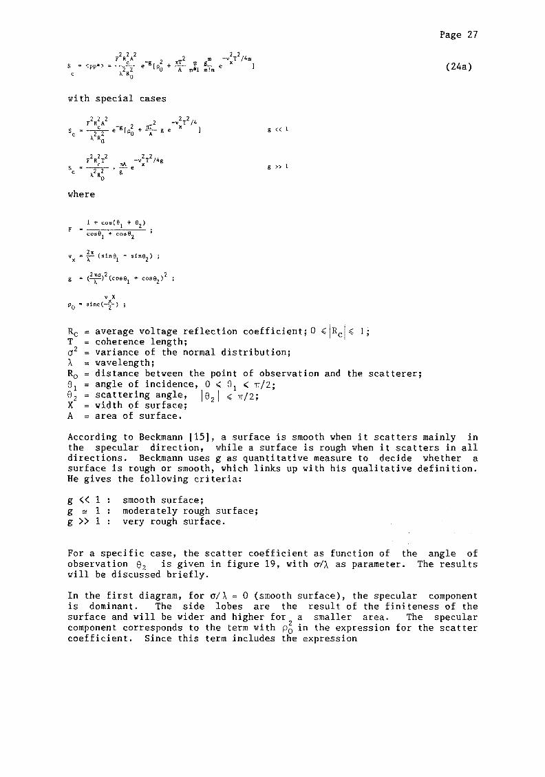
Re= average voltage reileetion coefficient; 0 ~!Rel~ 1; T coherence length; cr 2 = varianee of the normal distribution; À = wavelength; R0 distance between the point of observation and the scatterer; el = angle of incidence, 0 ~ el < rr/2; e2 scattering angle, I e2 j ~ rr/2; X width of surface; A area of surface.
Page 27
(24a)
According to Beckmann [15], a surface is smooth when it scatters mainly in the specular direction, while a surface is rough when it scatters in all directions. Beckmann uses g as quantitative measure to decide whether a surface is rough or smooth, which links up with his qualitative definition. He gives the following criteria:
g « 1 g ~ 1 g » 1
smooth surface; moderately rough surface; very rough surface.
Por a specific case, the scatter coefficient as tunetion of the angle of observation e2 is given in figure 19, with ~/À as parameter. The results will be discussed briefly.
In the first diagram, for a/À= 0 (smooth surface), the specular component is dominant. The side lobes are the result of the finiteness of the surface and will be wider and higher for a smaller area. The specular component corresponds to the term with p~ in the expression for the scatter coefficient. Since this term includes the expression

Page 28
40 40 fncidence ""' 43 fncidenc~ =- 43
<:Tf). - 0.00 o;A ~ 0.20 20
0 0
-20 -
-40 -40
-60 -60
-80 I 80
-90 -60 0 30 60 90 -90 -60 0 30 60 90
8 ----8---
2 2
40 40 .,....._ 'ndderce = 43 inc.idence ~ 43 o:l ~ 0.40 <:If). ~ 0.60 ~ 20- 20
+-' ç::
0 0 (]) •r-l t)
•r-l LH -20 LH
-20
(]) 0 t) -40 -40
":. (])
t: -60 -60 Cll t)
(/) -80 -80 I I I I
-90 -60 -30 0 30 60 <iO -90 -60 -30 0 60 <iO
82~ 82----
40 40 lnc iderH.: e =' 43 inddence 43
o-f), = 0.80 C!f).. = 1.00 20 20
0
-20 20
·40 -40
-60 -60
80 -80 - I
-90 -60 -30 30 60 90 -90 -60 30 30 60 90
8 2 --fillllooo. 8 ----2
Figure 19 Scatter diagrams according to expression (24).

Page 29
(25)
with an argument depending on the angle of observation, the successive side lobes have a different width.
For increasing o, the main lobe in specular direction becomes lower and wider, which indicates that the energy is scattered more equally into the various directions. In the diagrams 19e and 19f a small irregularity can be observed. This irregularity indicates the transition from the values found by use of expression (19a) to values found by expression (19c)
Comparison of the diagrams 19a and 19f raises questions. The total scattered power in diagram 19a seems to be more than in diagram 19f. Two remarks can be made on this observation.
First, the indication 'average reileetion coefficient' in (24) is misleading. Actually, this term is the average of the ratio of the reileetion coefficient and a normalization factor over the scattering surface, where the normalization factor depends on the rougness of the surface. The consequence is that the absolute level of the curves is not correct, because in generating these curves Re was assumed to be constant for any roughness. This point is discussed in more detail in appendix A.3.
Second, the diagrams given in tigure 19 represent the distribution of the scattered power in the plane of incidence. However, power is also scattered in lateral directions, out of the plane of incidence. So, if the total area in the diagrams decreases with increasing o/À this might indicate that more power is scattered out of the plane of incidence.
Still, the results might be useful, since it expresses the fact that for moderately rough surfaces the scattering in the specular direction is stronger than in non-specular direction. Therefore, some suggestions are given for implementation of (24) in a software simulation.
For simulation purposes, expression (24) is not very useful, for the calculation of the series in this expression entails a lot of work, especially in case g~ 1. Therefore the second term, representing the non-specular term, will be considered in more detail. A normalized representation of this part is given by the continuous lines in tigure 20, on a linear scale and for various angles of incidence. It appeared that the shape of these curves is closely approximated by the shape of the tunetion
g(8 2 ) = 4A.cosn(8 1-8 2)cos8 1cos8 2 {0 ~ 81 ~ rr/2, 81 - rr/2 & 82 ~ rr/2;
= 0 in all other cases.
(26)
The exponent n determines the width of these curves and is related to the roughness. A smooth surface means a large exponent, while a rough surface means a low value for the exponent. For very rough surfaces, the exponent becomes n=O and equation (26) becomes the expression of Lamhert's model (17).

exponent ~ 8 <.Ti).. ~ 0.60
/.
o.r
-90 -60 -30 0
exponent 8
I.
0.)
-90 -60 -30 0
exoonent 8 üjj 0.60
I.
os
-90 -60 -30 0
30 60 90
el~
30 60 oo
30
el-a-
60
I I I I I I I I I
90
exponent ~ 8
/. !f/) = 0.60
o.s
-90 -60 -30 0
exponent
o:.:~
oe;
I . oo -60 -30
8 0.60
Figure 20 Approximation of the scatter diagrams.
I I
I
I I
bO 90
el-a-
I
60 90
B:~, -e-
Page 30

Page 31
It is evident that the scatter diagram is not completely defined just by the shape of the curve, for no indication has been given about the absolute level of scattering. This level might be determined by integration of the mean scattered power over all directions and for that purpose a scatter diagram for the scattering in lateral direction, out of the plane of incidence, is necessary.

Page 32
6. SIMULATION
6.1. Introduetion
As mentioned in chapter 2, it would be of great help to be able to predict the impulse response of the mobile channel from environmental characteristics. To enable prediction, simulation software has been developed, using the results from the previous chapters. In this chapter, the global structure of the software will be elucidated, descrihing the functions of the various software modules.
6.2. Channel Simulation
6.2.1. Creation of a Database
The first step in the simulation is to create a database with the important characteristics of the mobile's environment. This entails the representation of each relevant scatterer in the direct neighbourhood of the mobile station and all buildings or clusters of buildings at a larger distance, which might be visible from the mobile's point of view. Every scatterer is determined by its height, length and its position relative to the base station. This position is defined by three parameters (X,Y,Y) in a two-dimensional Cartesian Coordinate system, with the base station in its origin and with the orientation initially free to choose (figure 21).
y
y -----------~-'--
bs ~----------~x~--------------- x
Figure 21 Definition of the position of a scatterer.
Furthermore, the height of the base station, being an important parameter, is entered into the database.

Page 33
6.2.2. Division into effective scattering elements
To be able to treat every scattering element as a distant scatterer, scatterers in the near field are divided into a number of effective scattering elements (ESES). Since our multipath analysis is performed mainly in two dimensions, the division in ESES is done only with respect to the length of the elements and not with respect to the height. For this case, the far-field criterion (22) is formulated as:
where: Ra= distance from mobile to scattering element; ~ length of scattering element; À = wavelength.
(27)
If the length does not satisfy (27), the element is divided into ESES which do satisfy (27). The determination of the number of ESES in each scattering element is the tunetion of the second module in the simulation software.
It should be remarked here that in the strict sense, the division in ESES, as described above, is not correct. Actually the division should also take place with respect to the height of the scatterers. This was omitted, to restriet the processing time. However it is recommended that in future implementations the multipath analysis is extended to three dimensions (including height).
6.2.3. Determination of valid propagation paths
If a propagation path is considered to be a conneetion between two ESES, a number of connections will be invalid. First, the conneetion should be between ESES which are not elements of the same surface as entered into the database. Second, the conneetion should have both its or1g1n and destination on the front of a scattering element. Third, the conneetion is only valid if it is not blocked by any other object. This blocking will be discussed in more detail.
If blocking occurs, the general situation is that only part of a scattering surface is shadowed by another object (figure 22).
In the simulation, however, blocking of all propagation paths between two ESES is assumed to occur when a conneetion between two elements is blocked by another object. If not, none of the propagation paths between the ESES are blocked. To represent the influence of height in this process, the conneetion is made between the tops of the two ESES to be connected.

Page 34
Figure 22 Partial shadowing.
Figure 23 Example of valid propagation path.
Page 35
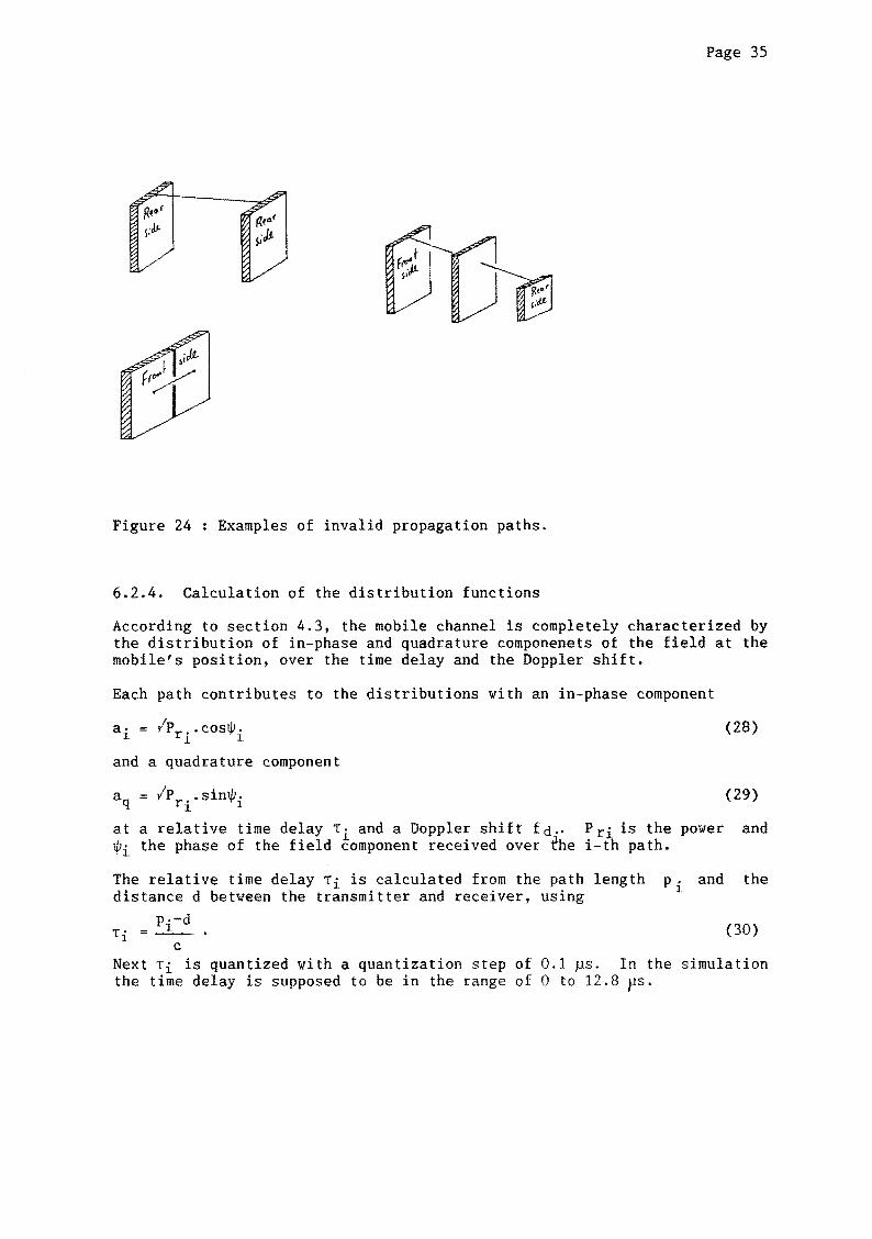
Figure 24 Examples of invalid propagation paths.
6.2.4. Calculation of the distribution functions
According to section 4.3, the mobile channel is completely characterized by the distribution of in-phase and quadrature componenets of the field at the mobile's position, over the time delay and the Doppier shift.
Each path contributes to the distributions with an in-phase component
a1• = /pr· .cos!J;.
1 . 1
and a quadrature component
(28)
aq = /Pri'sin!J;i (29)
at a relative time delay Ti and a Doppier shift fd·· Pr· is the power and tPi the phase of the field component received over the i-t~ path.
The relative time delay Ti is calculated from the path length p. and the 1 distance d between the transmitter and receiver, using
P·-d Ti = _!,__ • (30)
c Next Ti is quantized with a quantization step of 0.1 ps. In the simulation the time delay is supposed to be in the range of 0 to 12.8 ps.

Page 36
The ratio fd/v - known as the spatial frequency - is calculated from the angle of arrival and the wavelength using
fd/v = _!_ • cos a . (31) À
The spatial frequency fd/v is quantized with a quantization step 0.2 m- 1
and has a value in the interval [-3,3], since for 900 MHz 1/À = 3 m- 1•
The phase of the field component received is given by
1/Ji = Wc Ti + cjJ ' si (32)
where cp • s~
phase shift introduced by scattering.
For scattering in the non-specular direction by a rough surface, cjl 5 i should be a random variabie with uniform distribution over an interval witn length 2~, for the scattered field is incoherent. For smooth surfaces and for scattering in the specular direction by moderately rough surfaces, cjl 5 .
should have a quasi-constant value, representing coherent scattering. ~
Finally, the power received over a propagation path scattering, is calculated in an recursive process. process is the calculation of the flux in one point, another. Special cases are the start and the end of
with multiple order The basic step in this knowing the flux in the process.
For single order scattering, the step as mentioned above is executed only once. As an illustration, the calculation for single order scattering is considered in detail.
From 6.2.3., it is known which partial propagation paths are possible. So, with the base station or any effective scattering element as origin, all possible destinations are given.
The first origin is the base station. The first effective scattering element found from a scan for a possible destination is for instanee element number 4. The distance from the base station to this element is R04 • The flux at the position of this element is given by
where: - Pt - Gt - R
04
(33)
transmitted power; gain of transmitting antenna; distance from base station to scattering element 4.
Assuming that from the point of view of scattering element 4, the mobile station is a possible destination at a distance R0 m, the flux S2 at the position of the mobile is calculated using expression (23) for the scatter coefficient:
(34)
The power received at the mobile station can be calculated from
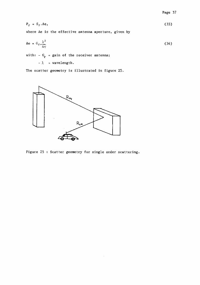
Pr = S2 .Ae,
where Ae is the effective antenna aperture, given by
wi th: - G r
- À
gain of the receiver antenna;
wavelength.
The scatter geometry is illustrated in figure 25.
Figure 25 Scatter geometry for single order scattering.
Page 37
(35)
(36)

Page 38
6.3. Filter simulation
As mentioned in chapter 2, the ability of a receiver to distinguish a propagation path in the impulse response of the mobile channel, depends strongly on the bandwidth of the receiver. Furthermore, unlike theoretica! impulses, pulses used in measurements have a certain width. Bath aspects, pulse width and limitation of the bandwidth of the receiver, are included in a filter simulation module which is added to the simulation software. The pulse shape and filter spectrum used in the simulation will be described in the following sections. But principally any pulse shape or filter might be implemented, depending on the purpose of the simulation. Our purpose is to be able to campare the results of the simulation with the results obtained by measurements of the impulse reponse. The choice of pulse shape and filter spectrum is made accordingly.
MOBILE CHANNEL
Fl L TER
Figure 26 Modules in simulation software
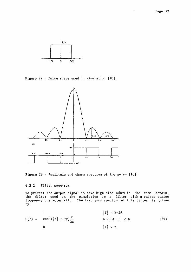
6.3.1. Pulse shape and spectrum.
--
The pulse used in the simulation is a rectangular pulse p(t) with width T and amplitude 1/T (figure 27):
p(t) 1/T (37)
0 !ti > t/2.
The spectrum of this pulse (figure 28) is the Fourier transfarm of p(t) given by
P( f) = sinc(TTfT) (38)
Page 39
I 11/r
l -T/2 0 Tf2
Figure 27 Pulse shape used in simulation [10].
-1/r 0 1/r 2'r 3/r r lbl
Figure 28 : Amplitude and phase spectrum of the pulse [10].
6.3.2. Filter spectrum
To prevent the output signal to have high side lobes in the time domain, the filter used in the simuiatien is a filter with a raised eosine frequency characteristic. The frequency spectrum of this filter is given by:
I )f) < B-2S S(f) = cos 2 (lf)-B+2S)..:!!.. B-2B ~ !fl ~ B 2B
(39)
0 lfj > B
Page 40
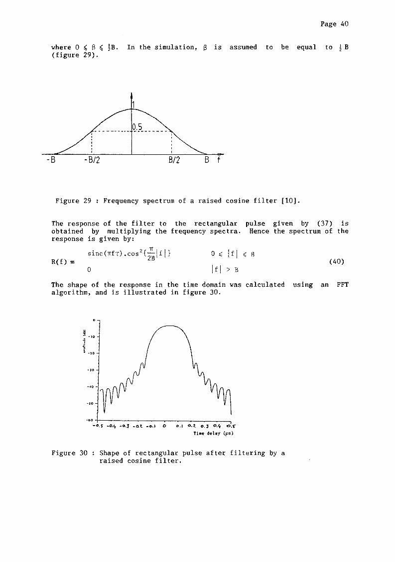
where 0 ~ B ~ !B. In the simulation, f3 is assumed to be equal to ~ B (figure 29).
1
-B - B/2 B/2 B f
Figure 29 Frequency spectrum of a raised eosine filter [10].
The response of the filter to obtained by multiplying the response is given by:
the rectangular frequency spectra.
pulse given by (37) is Hence the spectrum of the
sinc(rrfT).cos 2 {~!fl} 2B R(f)::
0
0 ~ lfl
lfl > B
~ B (40)
The shape of the response in the time domain was calculated using an FFT algorithm, and is illustrated in figure 30.
0
•10
•20
•SO
•60 -r-----~---.-----~~--.
Figure 30
-o.f -o.t, .o.J -o.t -o.l o o.1 o.t o.l o.t, c.r
Ti11e delay (ps)
Shape of rectangular pulse after filtering by a raised eosine filter.
Page 41
7. VERIFICATION
7.1. Determination of the scatter diagram of buildings by meesurement
In a densily populated area, it is rather difficult to find an isolated building from which the scatter diagram can be measured using a narrowband meesurement setup. The radio signal scattered by the target building interferes with the radio signal scattered by other objects and the resulting field is no measure for the field scattered by the target building. To prevent interference use can be made of a wideband meesurement setup, because in that case, as known from the previous chapters, the resolution in the time domain enables distinction of different propagation paths.
Another problem, the distinction of the signal scattered by the building from the signal received over the direct path can be solved using a directional antenna. In that case however the results of the meesurement should be processed to minimize the influence of the antenna gain pattern.
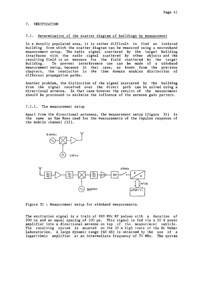
7.1.1. The measurement setup
Apart from the directional antennas, the meesurement setup (figure 31) is the same as Van Rees used for the measurements of the impulse response of the mobile channel (12].
Figure 31 Meesurement setup for wideband measurements.
The excitation signal is a train of 910 MHz RF pulses with a duration of 200 ns and an equal spacing of 100 ~s. This signal is fed via a 10 W power amplifier into a directional antenna on top of the measurement vehicle. The receiving system is mounted on the 50 m high tower of the Dr Neher Laboratories. A large dynamic range (60 dB) is obtained by the use of a logarithmic amplifier at an intermediate frequency of 70 MHz. The system

Page 42
allows registration of signals that exceed a level of -95 dBm. Using a transmitter power of 40 dBm and an antenna gain of 13 dB, this results in a maximum propagation loss of 148 dB.
Registration of the signals from the wideband receiver is realized by a wavefarm digitizer storing 512 data points at a sampling rate of 50 MHz. This means the starage of 10 ps of the signal corresponding to path length differences of up to 3 km. The maximum meesurement repetition rate, which is determined by the data transfer to a hard disk, is 50 Hz.
7.1.2. Results
The receiving system as described above triggers on the first impulse received with a level higher than -60 dBm. This feature appeared to be the cause of results which are of little value, for two reasons. First, the measurements were disturbed by an unknown radar signal covering at least the 900 MHz frequency band. This caused so many false triggers (figure 32) that the data obtained are not enough to define a scatter diagram. But even in absence of this interferer, the analysis of the results would have been a problem, for if the signa! scattered from the target building comes below the trigger level it would not be detected.
ê -M m ~ ~
~ -~0 ~ ~ 0 ~
-~
-~
-~
-Qo
-~0
Relative time delay (~s)
Figure 32 Example of a false triggered measurement.
Both problems can be solved by introducing a triggering absolute in time, using two stable oscillators: one in the receiver and one in the transmitter. However there was not enough time left to implement this new trigger concept within the time of this study. So no results are available on the meesurement of the scatter diagram of a building.

Page 43
7.2. Verification of the simulation software
From chapter 4, it is known that the transfer of a (wideband) radio signa! by a mobile channel is completely characterized by four parameters: phase, Doppier shift, time delay and received power. To verify the model, the calculated values of these parameters should be compared with measured values.
A large amount of data is available on impulse responses of the mobile channel, obtained by measurements which were performed by Van Rees [12]. These data contain two of the four parameters: the received power as function of the relative time delay. It should be noted that during his measurements Van Rees also experienced interference, but this interference was present during short periods only. In our case however, the interference was present continuously.
Initially, it was assumed that the Doppier spectrum could the successive impulse responses. However, it has section 4.2. and 5.2. that this is only possible in the coherent scattering is dominant.
be retrieved from become clear from situations where
So the only verification possible is a discussion of the results obtained by simulation of some simple situations, and a comparison of a measured impulse response with the impulse response obtained by simulation using an abstract representation of the rnabile's environment.
7.2.1. Simulation of a fictive situation
First situation to he considered is the situation where two scattering surfaces are located symmetrical with respect to the line m between the base station and the initia! position of the mobile station (figure 33).
~·-·-·-·-·-~·-·-·-·-·-·_J BS MS
/ Figure 33 Simple situation simulated.

Page 44
Two cases are considered. The first with the mobile moving perpendicular to m and the second with the mobile moving along m. The discrete impulse response, which is identical for both situations, is given in figure 34. The response of the channel followed by a band filter with a bandwidth of 20 MHz is given in figure 35.
In the discrete impulse response four lines can be distinguished. The one at the left most side corresponds to the direct path. The offset from L=O ps is caused by the quantization of the time delay. The second line is the contribution of the scattering surfaces after single order scattering. This line consists of two components each coming from another direction. The same is true for the two lines near T=l ps, which represent the contribution of the double scattered waves.
If the continuous impulse response obtained by filtering is considered, we see that the first paths still can be distinguished. The paths arriving at a time delay near T=l ~s however combine into one pulse in the continuous response.
The Doppler spectra for both cases are given in figure 36 and 37, for a mobile station moving at a speed of 30 m/s. Figure 36 represents the spectrum for the case of the perpendicular direction of movement. The line at fd=O Hz corresponds to the direct path, while the lines at ! 90 Hz represent the contributions from the scatterers. Figure 37 represents the spectrum if the mobile moves along the line m. The line corresponding to the direct path is shifted to 90 Hz, while the other lines are replaced to the region near fd=O Hz. The reason will be clear from figure 33.
The tap in the discrete impulse response, representing the contributions between T = 0.3 0.4 ps, is considered in more detail for subsequent impulse responses. The tap signal for perpendicular movement is given by figure 38. Strong fading is observed with a period of !À· This result was expected from the fact that coherent scattering was assumed. In figure 39, the signal on the same tap for movement along m is given. Here the fading rate is much lower (l/2À). These results are not spectacular. They only confirm that the software operates as it should. The validity of the model is a totally different issue.

--30-e "' ..., :-40-. J 0 Q. -50 -
-60 -
-70-
-eo -
-'10
100 ~----,~~~--~~--,-,--,1---,lr---lr---.1---~.--,-,--., -I 0 2 3 4 5 6 7 8 9 10
IIma deloy I~A•l
Figure 34 Discrete impulse response of the simulated channel.
Ê 0
(Q
~-IC
; -20 0 Q.
-30
-40
-50
-60
-7G
eo
-90
-100 I -I 0
tlma deloy (I',J
Page 45
Figure 35 Impulse response of the channel followed by a bandfilter.

- 30-E
"' .."
:-40-. l 0 0.-50 -
-bO -
-70 -
-eo -
-100 4-----~-L----.-~----,,------~----.-,-----.-,--~ 120 -90 -1>0 -30 0 30 óO 90
Doppier >hift (Htl
Figure 36 Doppier spectrum for movement perpendicuiar to m.
--30 -E
"' .."
:-40-• J 0 0.-50 -
-60 -
-70 -
-eo -
-90 -
-100 4-------r-~----,,,-----,,--~-L4-----~,------~,----~ -120 -90 -60 -30 0 30 60 90
Doppier shil; (Hz)
Figure 37 Doppier spectrum for movement along m.
Page 46

:;; -50 ): 0 a.
Figure 38
:;; -50 ): 0 a.
Figure 39
0.3- O.t.,f<~
I 0 Á. displacement
Tap signal for movement perpendicular to m.
bA
0.3- 0.<,,.~
I 0 Á.
displacement
Tap signal for movement along m.
Page 47

Page 48
7.2.2. Simulation of a real situation
Finally the simulation of a measured impulse response and is given in figure 40. figure 41.
measured impulse response is presented. The is obtained from the data provided by Van Rees
The simulated impulse response is presented in
Comparing the two impulse responses, we may conclude that the simulation is more realistic than the one presented in chapter 5. The shape of the simulated impulse response shows a good resemblance with the measured response. Apparantly, an important souree of scattering has been omitted, for in the simulation no response is found between 1.3 and 1.9 ps. The strong response near 7 ~s is caused by second order scattering. In reality, this response appears to be much lower. This difference might be explained by the fact that for second order scattering the effective area of the buildings involved in the process is smaller than assumed. Again it is stressed that this result is not an assurance for the validity of the model. A proper verification is only possible if more information on the measured data becomes available.

Page 49
! 11
6 t ~ ~ 10
Time delay (ps) __.
Figure 40 Impulse response obtained by measurement [12].
0 E
a:l
~-10 -
~ -20 0 0 -30
-40
-50
-60
-70
-eo
-90
-100 I
0 3
time delat (,usl
Figure 41 Impulse response obtained by simulation.

Page 50
8. CONCLUSIONS AND RECOMMENDATIONS
The objectives of the study to this thesis were to verify whether the mobile radio channel can be simulated usefully from characteristics of the mobile station's environment by a relatively simple model, to obtain insight into the consequences of the Doppler shift for the impulse response of the mobile channel, and to develop simulation software for use in system performance analyses. It was not the objective to obtain deterministic predictions for all situations possible, but just to get an impression of the values and variabilty of the parameters characterizing the mobile channel for typical situations.
After an orientation in the theory on multipath propagation, the study concentrated on the scattering of radio waves by buildings. The basic idea was to assign a scatter diagram to each relevant building in the mobile's environment. Much attention has been given to the distribution of the scattered power over the possible scatter directions, but the influence of the scattering on the phase of the signal was initially left out of consideration. Only in the last part of the study the importance of this point was recognized.
Fortunately this does not mean that the results found for the diagrams of the scattered power are of no value. On the contrary. The issue of coherent or incoherent scattering gives additional information, and provides an extra criterion on which a model for the scattering from buildings can be judged.
According to Beckmann, very rough surfaces scatter incoherently in all directions. Moderately rough surfaces scatter coherently in a narrow cone about the specular direction, but incoherently in the other directions and a perfectly smooth surface scatters coherently. According to this theory no technique using the coherence of the phase may be implemented for mobile communications in an environment with only rough surfaces. But since we know that in a mobile environment communication using phase modulation techniques is possible, it may be concluded that at least for some time, a sufficient part of the waves is scattered coherently. From this it may be concluded that an ideal rough surface is not an adequate model for a building's surface.
Since the relation between incoherent scattering and rough surfaces was not recognized until the last part of the study, Lamhert's model for diffuse scattering was implemented in the simulation software, whereas the phase was supposed to be coherent, i.e. dependent only on the path length from the transmitter to the receiver via the mean plane of the scattering surface.
It has become clear that the question whether the scattering is coherent or incoherent is very important. Therefore, it is strongly recommended that wideband measurements like performed by Van Rees [12], are analyzed tapwise, i.e. that data at the same relative time delay of subsequent impulse responses is compared. A more or less regular fading pattern on one or more taps would indicate dominant coherent scattering. It should be taken care of that the interval between the measured impulse responses is

Page 51
small enough to detect possible fading. From experiences with the simulation software, it appeared that the distance between two positions at which the impuise response is measured must be in the order of a tenth of a waveiength, in order to detect possible fading dips.
Furthermore, measurements of the scatter diagram of buildings at 900 MHz are suggested to check whether or not one or more dominant scatter directions can be found. Dependent on the result of these measurements, the surface of the building may adopted to be moderately rough or to exist of smooth elements. Whatever the final choice, the basic structure of the simuiation software seems to be suitable for implementation.
In the present form, the software can be used to determine the influence of the Doppler shift on the phase and time delay associated with the signal received over each propagation path. However, this does not mean that the phase shift nor the change in time deiay can be predicted from the Doppler shift, for incoherent scattering may annul the infiuence of the Doppler shift.
In theory the determination of the Doppier spectrum from measured impulse responses is possibie, but oniy under strict conditions. Since it appeared to be easier to determine the Doppier shift from the phase, it is recommended that complex impulse responses are measured [18].

LITERATURE
[1] CEPT/GSM/WP2: COMPARISON OF MOBILE RADIO SUB SYSTEMS, Report WP2/1, rev.2, March 1986.
[2] Lee, w.c.Y.: MOBILE COMMUNICATIONS ENGINEERING, McGraw-Hill, Inc., 1982.
[3] Okumura, Y. et al.: FIELD STRENGTH AND lTS VARIABILITY IN VHF AND UHF LAND MOBILE SERVICE, Rev. Elec. Comm. Lab. 16, pp. 825-873, September 1968.
[4] Hatta, M.: FORMULA FOR PROPAGATION LOSS IN LAND MOBILE RADIO SERVICES, IEEE Trans. on Vehicular Technology, vol. 29, pp. 317-325, August 1980.
[5] Cox, O.C. and Leek, R.P.: DISTRIBUTION OF MULTIPATH DELAY SPREAD AND AVERAGE EXCESS DELAY FOR 910 MHz URBAN MOBILE RADIO PATHS, IEEE Trans. on Antennas and Propagation, vol. 23, pp. 206-213, March 1975.
[6] Turin, G.L.: A STATISTICAL MODEL OF URBAN MULTIPATH PROPAGATION, IEEE Trans. on Vehicular Technology, vol. 21, pp. 1-9, January 1972.
[7] Jakes, W.C.: MICROWAVE MOBILE COMMUNICATIONS, John Wiley & Sans, Inc., 1974.
[8] Rees, J. van: PROPAGATION ASPECTS OF LANDMOBILE RADIO SYSTEMS IN BUILT-UP AREAS, Dr. Neher Laboratories, Report 545 TM/86, May 1986.
[9] Parsons, J.D. and Bajwa, A.S.: WIDEBAND CHARACTERIZATION OF FADING MOBILE RADIO CHANNELS, lEE Proc., Vol. 129, Pt. F, No.2, April 1982.
[10] Shanmugan, K.S.: DIGITAL AND ANALOG COMMUNICATION SYSTEMS, John Wiley & Sans, Inc. 1979.
[11] Proakis, J.G.: DIGITAL COMMUNICATIONS, McGraw-Hill, Inc., 1983.

[12] Rees, J. van: MEASUREMENTS OF THE VIDEBAND RADIO CHANNEL CHARACTERISTICS FOR RURAL, RESIDENTlAL AND SUBURBAN AREAS, COST 207 TD (86), April 1986.
[13] Ikegami, F. and Yoshida, S.: ANALYSIS OF MULTIPATH PROPAGATION STRUCTURE IN URBAN MOBILE RADIO ENVIROMENTS, IEEE Trans. on Antennas and Propagation, vol. 28, pp. 531-537, July 1980.
[14] Rees, J. van: MEASUREMENTS OF IMPULSE RESPONSE OF A VIDEBAND RADIO CHANNEL AT 910 MHz FROM A HOVING VEHICLE, Electronic Letters, Vol. 22, no. 5, February 1986.
[15] Beckmann, P. and Spizzichino,A.: THE SCATTERING OF ELECTROMAGNETIC WAVES FROM ROUGH SURFACES, Pergamon Press, 1963.
[16] Clarke, R.H. and Brown, J.: DIFFRACTION THEORY AND ANTENNAS, Ellis Horwood Ltd., 1980.
[17] Bramley, E.N. and Cherry, S.M.: INVESTIGATION OF MICROWAVE SCATTERING BY TALL BUILDINGS, IEE Proceedings, vol. 120, pp. 833-842, August 1973.
[18] Cox, D.C: DELAY DOPPLER CHARACTERISTICS OF MULTIPATH PROPAGATION AT 910 MHZ IN A SUBURBAN MOBILE RADIO ENVIRONMENT, IEEE Trans. on Antennas and Propagation, vol. 20, pp. 625-635 , September 1972.
[19] Deryugin, A.: THE REFLECTION OF A LATERALLY POLARIZED PLANE WAVE FROM A SURFACE OF RECTANGULAR CORRUGATIONS, Radiotekhn.15, no.2, pp. 15-26, February 1960.
[20] Abramowitz, M. and Stegun, I.A.: HANDBOOK OF MATHEMATICAL FUNCTIONS, Dover Publications, Inc., New York, 1972.

APPENDIX A
Scattering from rough surfaces
In this appendix a derivation wil! be given of the general Kirchhoff
solution forscattering from rough surfaces according to [15]. The result
wil! be applied to a specific model of the surface's roughness, i.e. a
surface with a height which is normally distributed.
A.l General Solution:
The surface S is described in a Cartesian coordinate system x, y, z, with
unit veetors e , e and -x -y
• The height of the surface is given by the
function z = Z(x,y). The mean level <Z>, defined by
<Z> 1 A JJ Z(x,y)dxdy,
s (Al)
is assumed to be equal to zero: <Z>
S on the xy-plane.
0. A is the area of the projection of
The time Fourier transform of the incident field E. has a magnitude E. given -1 1
by:
-jk .. r --1_ -
e
where k. is the propagation vector of the incident field, with --1_
(A2)
(A3)
The angle of incidence, included between the direction of propagation ~i
and , wil! be denoted by e1 (figure A.l).
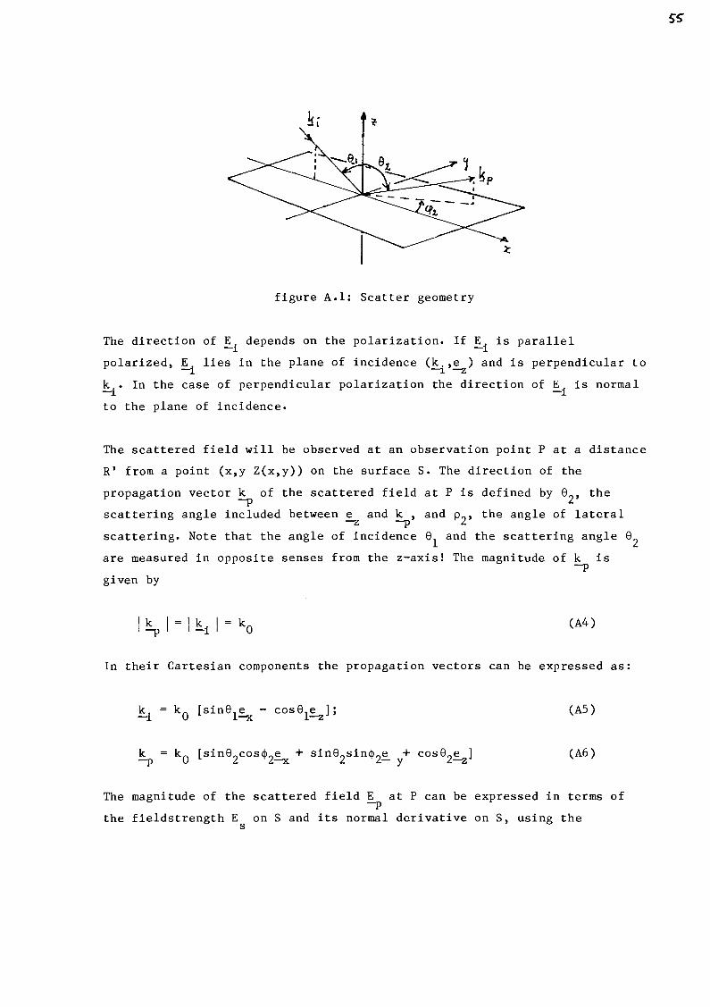
figure A.l: Scatter geometry
The direction of E. depends on the polarization. If E. is parallel -]_ -1
polarized, E. lies in the plane of incidence (k.,e) and is perpendicular to -]_ -]_ -z k .• In the case of perpendicular polarization the direction of E. is normal -]_ -1
to the plane of incidence.
The scattered field will be observed at an observation point P at a distance
R' from a point (x,y Z(x,y)) on the surface S. The direction of the
propagation vector ~ of the scattered field at P is defined by e2
, the
scattering angle included between e and k , and p2
, the angle of lateral -z -p
scattering. Note that the angle of incidence e1
and the scattering angle e2
are measured in opposite senses from the z-axis! The magnitude of k is -p
given by
I ~ I = I ki I = ko (A4)
In their Cartesian components the propagation veetors can be expressed as:
k. -]_
(A5)
(A6)
The magnitude of the scattered field E at P can be expressed in terms of -p
the fieldstrength E on S and its normal derivative on S, using the s

Helmholtz integral:
1 E = - ff (E 'VQ; - <jiVE ) .n dS,
p 4n; s s- - s -
where, according to Huygens' principle, 4 is given by
1
4 = R'
(A7)
(A8)
2A * If P is moved to the Fraunhofer zone of diffraction (R' ~-x ) , R' can be
expressed as
R' 1
Ra - k (k • r), a-p- (A9)
where Ra is the distance from P to the origin and r is the position vector
of the point (x,y, Z(x,y)) on S (figure A.2).
Figure A.2: Derivation of (9)
Since for the Fraunhofer zone Ra >> r , 4 can be expressed as
oE The exact values of Es and ons are in general unknown. The Kirchhoff method
consists essentially in approximating these values by the values associated
with the field on a tangent plane at the point under consideration.
* Rayleigh's far-field criterion [16]

Principally this approximation is only valid when the surface does not
contain a large amount of sharp edges, sharp points or other irregularities
with small radii of curvature. However, a comparison with the results of an
exact theory on scattering by a surface consisting of rectangular
corrugations, devellop by Deryugin [19] shows that the Kirchhoff metbod may
still be a good approximation when edges are present.
Within the approximation, the field on the surface S may be expressed as the
sum of the incident field on S and the reflected field on s.
The incident fieldstrength, given by (AZ), is
-jk .• r --1_ -
Ei = e
the reflected field can be expressed as
E r
-jk .• r R
--1_ -s .e
= R.e
where:
w = k - k • - -i -r'
-jw.r --s
j(k • -r
- k .r) -r-
• e
-jk .r -r-
• e (All)
r = position vector of the local point of reflection; -s k
1 propagation vector of the incident field;
k propagation vector of the reflected field; -r
R = reflection coefficient of the tangent plane.
The fieldstrength on S is found by substituting r =
incident and reflected field:
E. + 1, s 's
E. (l+R) l,S
r and adding the -s
(Al2)

The normal derivative of the field on S is found by differentlating the
incident and reflected fieldstrengths:
oE. on
1 = _yE i •!!. = -jE i ( k i . !!_) (A13)
and
oE _r = VE .n = -jE (k .n) on - r- r -r-
(Al4)
Since (k .n) = -(k .• n) (figure A.3), the normal derivative of the field on -r - -:I. -
S is given by
oE (::..n)S = -j(E. k .• n + E k .n)
v 1,s -:~. r,s -r -
= -j(l-R)Ei k .• n ,s -:I. -(AlS)
Figure A.3: Reflection by a tangent plane
Differentlating (AlO) gives
o(ji = 'Jq,.n = j(ji(k .n) (Al6) on-- -p-
Substitution of (Al2), (AlS) and (Al6) in (A7) gives
E = j_ ff [E. <P(l+R)k .n = E. (ji(l-R) k .• n] dS p 4n: s 1, s -p - 1, 6 -1 -
Defining
V = k - k - -i -p n = k. + k 1>- -1 -p
(Al7)
(Al8)

and using (A2) and (AlO) yield
where
r -s
-jkORO
E .e JJ (R~ - .E_).!!.. e -J 4rcR0 p s
in Cartesian coordinates
xe + ye + Z(x,y)e ; -x -y -z
-jv.r --s
dS ,
n 1
=- {- sina:cos~e - cosasin~e + cosacos~e } n -x --y -z
n
dS
tana
tan~
2 2 2 )1/2 (sin acos ~ + cos a
-1 (cosacos ~) dxdy
z1 x
zl y
Substitution of (AS) and (A6) in (Al8) and defining a, b and c as
gives
a (l-R)sin81 + (l+R)sin8 2cos~2 b
c
(l+R)sin82sin~2 (l+R)cose2 - (l-R)cose1
(R~ - .E_). g_dS ko
(aZ 1 + bZ 1 - c)dxdy
n x y
(Al9)
(A20)
(A21)
Using A(21) and assuming the projection of S on the xy-plane to be
rectangular, stretching out from -X/2 to X/2 and from -Y/2 to Y/2 yield
E p
-jk 0
X/2 Y/2
J J -X/2 -Y/2
1 I [aZ 1 + bZ - c]
n x y
-jv.r - -s e dxdy (A22)
For the time being the factor in front of the integral will be considered to
be a constant:
K (A23)

Substitution in (A22) gives
E p
X/2 Y/2 1
-jv.r --s
K J J {az 1 + bZ 1 - c} e dxdy
-X/2 -Y/2 n x y
-jv.r Partial differentiation of e --s to x and y respectively gives
With
-jv.r V -jv.r +l
-jv.r Z1 (x,y)
- -s x --s à
--s e -- e e x V V x
z z
-jv.r V -jv.r +l
-jv.r Z1 (x,y)
--s - _z. e - -s à
- -s e e y V V y
z z
(A25), (A24) can be expressed as
E p
X/2 Y/2 1
av + bv -jv.r K J J - (c + _x __ --"-Y) e - -s dxdy
-X/2 -Y/2 n vz
Y/2 -K f
-Y/2 j a
nv z
X/2 d y f
-X/2 d e
X/2 Y/2 -K f j b d x f d
-X/2 nvz -Y/2 e
-jv.r --s
-jv.r --s
(AS), (A6), (A18) and (A20) give
c +
Defining
F
and
e(X,Y)
av + bv x y
V z
Y/2 -K j
-Y/2 j a
nv z
1 + cos81cose2 - sin81sin82cos~2
cose1 + cose2
X/2 d y f
-X/2
-jv.r X/2 Y/2 d e - -s_K J j b d x J
-X/2 nvz -Y/2 d e
6o
(A24)
(A25)
(A26)
(A27)
(A28)
-jv.r --s
(A29)

(A25) can be written as
E p
X/2 Y/2 -jv.r
f f R --s 2K.F - e dxdy + e(X,Y) ,
-X/2 -Y/2 n (A30)
where R and n depend on the material characteristics of the surface and on
the slope at a specific point of the surface.
So, if the scatter coefficient p is defined as the ratio of the scattered
field to the incident field, p can be expressed as
X/2 Y/2 R -jv.r f --s
2K.F. f - e dxdy + e(X,Y) -X/2 -Y/2 n
(A31)
(A31) is the general Kirchhoff salution for the scattering from rough
surfaces, from which the scattering coefficient can be determined if Z(x,y)
is given.
To be able to solve the integral, the ratio ! will be approximated by the n
average of this ratio over S:
R c
<R/n> -l X/f2 Y/2 R
f - dxdy A -X/2 -Y/2 n
and can be written in front of the integral.
(A32)
By introduetion of this average in the ratios a/n and b/n and by defining
(A29)
a c
b c
<a/n>
<b/n>
can be written as
a Y/2 e(X,Y) -K . c f J-
V z -Y/2
b X/2 -K . c f Jy
z -X/2
(A33)
X/2 -jv.r dy f --s
de -X/2
Y/2 -jv.r dx f --s
de (A34) -Y/2
~I

e(X,Y) is an edge effect, which will be shown negligible when compared to
the first term for A >> À2.
Let S be an arbitrary surface of large dimensions (X >> À, Y >> À). Let S'
be identical with S everywhere except near the edges x = + X/2 and
y = ~ Y/2, where it continuously approaches the value Z = 0. Then forS',
using (A34), e(X,Y) can be expressed as
e(X,Y) a b
4K ( ~ + ~} • sin(v X/2) • sin(v Y/2) V V V X y
z y x
For the specular direction (v = v = 0) e(X,Y) vanishes. x y
(A35)
For v and v * 0, X or Y is decreased by slicing strips from the surface x y
S', until e(X,Y) vanishes. Since v and v contain the factor k0
, the x y
necessary decrease will be À at most.
S is identical with S' over an arbitrarily large area except for the narrow
strips at the edges. Hence, it is physically clear that the two surfaces
will also have practically the same scattered field, so for A = XY >> À2
e(X,Y) is always negligible.

A.2 Rough surfaces as random processes
Principally, the surface of a building can be described exactly. Therefore
it is possible to give an exact expression for the scatter coefficient,
using the general Kirchhoff solution. In practice however, the determination
of the surface function Z entails so much work, that it is more convenient
to assume the surface to be given by a random stationary process.
Two functions are needed to describe the characteristics of the surface. The
probability density function w (z) gives the probability of a deviation z
z = Z(x,y) from a mean level < Z >. The normalized correlation function or
autocorrelation coefficient is a measure for the concentration of
irregularities.
Let the mean level of the surface, defined by (Al), be
< z > 0 (A36)
and assume R/n to be constant over the surface S (e.g. the average over S).
Furthermore, assume S to be large enough to neglect the edge effect term in
(A31). Then the mean value of the first term in (A31) can be expressed as
< p > X/2 Y/2
< 2K.F f f -jvr
s R/n e dxdy > -X/2 -Y/2
2K.F .R c
X/2 Y/2
f f -X/2 -Y/2
-j(v x+v y) -jv z x y < z > dxdy e e
The characteristic function x(v ) of the surface is defined by z
x(v ) z f
-CD
-jv z w (z) e z dz
z
-jv z < e z >
Substitution in (A37) gives
< p > 2K.F.R • x(v ). c z
X/2 Y/2 f f
-X/2 -Y/2
-j(v x+v y) e x y dxdy
(A37)
(A38)
(A39)
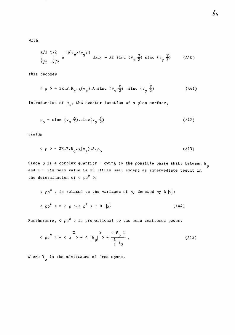
With
X/2 Y/2 J J
-j(v x+v y) e x y dxdy XY sine
X/2 -Y/2
this becomes
Introduetion of p , the scatter function of a plan surface, 0
P = sine 0
yields
< p > = 2K.F.R •X(v ).A.p c z 0
(A40)
(A41)
(A42)
(A43)
Since p is a complex quantity - owing to the possible phase shift between E p
and K - its mean value is of little use, except as intermediate result in
the determination of < pp* >.
< pp* > is related to the varianee of p, denoted by D ~}:
< pp* > < p >· < p* > + D {p}
Furthermore, < * > is proportional to the mean scattered PP
* 2 2 < p >
< pp > < p > = < !Epi > = E 1 2 Ya
where Y is the admittance of free space. 0
(A44)
power:
(A45)
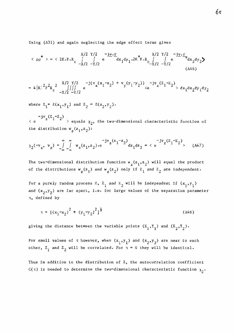
Using (A31) and again neglecting the edge effect terms gives
* < PP > = < 2K.F.R c
X/2 Y/2
f f -X/2 -Y/2
-j(v (x -x ) + v (y 1-y2)) -jvz(Z 1-z 2) e x 1 2 y <e > dx 1dx
2dy 1dy
2
where Z
-jv (Z -z ) < e z
1 2 > equals x2, the two-dimensional characteristic function of
the distribution wz(z 1 ,z 2):
Xz(-v , v ) z z f "'
-jv (Z -z ) < e z 1 2 > (A47)
The two-dimensional distribution function wz(z1
,z 2) will equal the product
of the distributions wz(z 1) and wz(z 2) only if z1 and z2 are independent.
For a purely random process Z, z1
and z2
will be independent if (x1,y
1)
and (x2,y2) are far apart, i.e. for large values of the separation parameter
-r:, defined by
(A48)
giving the distance between the variable points (X1
,Y1
) and (X2
,Y2).
For small values of 1: however, when (x1,y
1) and (x
2,y
2) are near to each
other, z1
and z2 will be correlated. For -r: = 0 they will be identical.
Thus in addition to the distribution of Z, the autocorrelation coefficient
C(-r;) is needed to determine the two-dimensional characteristic function Xz•

By definition C(~) is given as
<Z1Z2>- <Z1><Z2>
2 2 <Z1 > - <Z1 >
(A49)
Due to (A36), this reduces to
(ASO)
with
lim C(~)= 1, full correlation, linear dependence; ~-+-CD
lim C(~)= 0, independence. ~-+-CD
For a purely random surface, C(~) will decrease monotoneously from its
maximum value C(0)=1 to C(CD)=O. The distance T for which C(~) drops to the -1
value e is called the correlation distance.
Substitution of (A39), (A46) and (A47) in (A44) gives the varianee D {p}:
D {p}
(A51)
With p
D {p} y 1+Y/2 . ( p+ ) -J V V q J e x y
y1
-Y/2
* [x2(-v ,v )-x(v )·X (v )] dx1dy 1dpdq z z z z (A52)
Since the term between square brackets is only relevant in the region ~0
and ~0, the integration limits may be extended to infinite.

This yields:
Y/2 CD -j(v p+v q) f ff e x Y [x2(-v ,v )-x(v ).x*<v )]dx
1dy
1dpdq
-Y/2 -CD Z Z Z z
Integration over x1
and y1
gives
D {p} CD -j(v p+v q)
ff e x Y [x2(-v ,v )-x(v ).x*<v )]dpdq z z z z -oo
Transformation from Cartesian to polar coordinates,
p= 'tCOS<fl
q= ,;sin<P
results in
(A53)
(A54)
(ASS)
oo 2rc -j,;(v cos<t>+v sin<t>) * f f e x Y [x2(-v ,v )-x(v ) x(v )],;d,;d<t> 0 0 z z z z
The term between square brackets is independent of 4>·
With
2rc J e-j(xcos<P + ysin<P) d4>
0
2 2 2 re J
0 ( I x +y ) [20]
where J0(.) is the Bessel function of the first kind and zero order,
(ASS) gives
D {p} (A57)
where vxy

At this point the general approach is left and attention will be focussed on
a specific kind of distribution w (z) and a specific autocorrelation z
coefficient C(~).
Most appropriate distribution is the normal distribution, for as any
varianee may be chosen to represented the degree of roughness and any
correlation distance to repreaent the density of irregularities, this will
nat mean a great loss of generality.
Let the distribution of Z be given by
w (z) z
2 2 1 -z /2 cr
= o /21t e (A58)
The standard deviation cr, which in this case is also the root-mean-square
value of Z, is a measure for the roughness of the surface. A large cr
corresponds to a large roughness. When cr ~ O, (A58) will tend to the dirac
function and Z will cease to be a random variable, implying a smooth
surf ace.
By (A38), the characteristic function associated with the normal
distribution is
1 2 2
x(v) 2 vz (J
= e
As auto-correlation coefficient the function
Ch) 2 2
-~ /T = e
is chosen, where T is the correlation distance.
(A59)
(A60)
The two-dimensional normal distribution of two random variables z1
and z2
,
with mean values zero and varianee cr2
, and correlated by a correlation
coefficient C, is
1 (A61) e
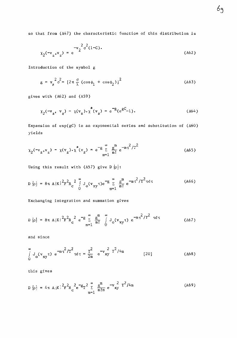
so that from (A47) the characteristic function of this distribution is
x2(-v ,v ) z z
e
2 2 -v2
a (1-C).
Introduetion of the symbol g
gives with (A62) and (A59)
* x2(-vz, V ) - x(v )·X (v ) z z z
(A62)
(A63)
(A64)
Expansion of exp(gC) in an exponential series and substitution of (A60)
yields
* oo m 2 2
e-g E lL -m.,; /T X (-v V ) - x(v )•X (v ) 2 z' z z z m=l m! e
Using this result with (A57) give D{p}:
D {p} 2 2 2 oo _ oo m 2/ 2 = 8n AIKI FR J J (v -r)e g .E mg.' e-m-r T .,;d.,;
c 0 o xy m=l
Exchanging integration and summation gives
oo m oo
D {p} = 8n AIKI2F2R 2 e-g E g J J (v -r)
c m! o xy m=l 0
and since
oo -ml/T2 T2 J J ( v 1:) e -rd.,; = -0 o xy 2m
this gives
-v 2 T2/4m e xy
2 2 -m.,; /T -rd-r e
[20]
(A65)
(A66)
(A67)
(A68)
(A69)

Three cases will be distinquished
1) g<<l, slightly rough surface or bath e1 and e2 grazing angles;
2) g=l, moderately rough surface;
3) g>>l, very rough surface.
g<<l: only the first term of the series is important
D {p} (A70)
~1: in this case (A69) may still be used with a reasonable number of terms.
g>>l: in this case (A69) has a great number of relevant terms and converges
too slowly to be of any practical use. Therefore integral (A57) will be
considered again.
Substitution of (A64) and (A60) in (A57) gives
D {p} (A71)
For g>>l this integral receives significant contributions only from the
-.,;2/T2 region near .,;=0. Hence e may be approximated by the first two terms of
the exponentlal series:
(A71) and (A72) give
D {p}
For large g (A73) reduces to
D {p} J J (v .,;) 0
o xy
2 2 -g.,; /T d e .,; .,;
(A72)
(A73)
(A74)

With (A68), (A74) becomes
D {p} (A75)
* Now consider the quantity < pp >, given by (A44) as
* < pp > * <p>.<p >+D{p}
which according to (A45) is proportional to the mean scattered power.
(A43), (A59) and (A63) give:
<p> (A76)
Substitution of (A76) in (A44) yields
* 2 2 2 2 2 -g < pp > = 4 IK I F R A p e + D {p} c 0
(A77)
Thus the mean power scatter coefficient can be found using the following
expression:
* < pp
With special cases
* < pp
* < pp > g
2 2 -v T /4g
ne xy
oo m 2 2 lL_ -v T /4m]
E m!m e xy m=l
(A78)
(A79)
g»l (A80)
* Note that to find (A80) the approximation < pp > "" D {p} for g»l has been
used.

A.3 Results and discussion
Substitution of (A23) in (A78) gives the result of the derivation of the
scattercoefficient S for the mean scattered power in the plane of c
incidence:
s <pp*> c
with special cases
F2R2 A2 -g 2 2
c + nT g e s = À_2R2 e [po c A
s c
where
F =
0
F2R2T2 2 2 ïlA -vxT /4g c
À.2R2 -e g
0
1 + cos(el + e2)
cosel + cose2
2n ( . e . e ) vx = s~n 1 - s~n 2 ;
V X x
Po sinc(-2-)
-v2
T2
/4 x ]
R = average reflection coefficient 0 c
T = coherence length ; " IR I ~ c
2 varianee of the normal distri bution (j
À. = wavelength ;
1
Ro di stance between the point of observation
el = angle of incidence 0 "; el .;;; n/2
e2 angle of scattering -n/2 " e2 "
n/2
x width of the surface
A = area of the surface.
(A81)
g « 1
g » 1
and the scatterer
The results will be discussed here, especially with respect to the influence
of the parameters R , F and g. c
R is the average of the ratio R/n over the surface. It was introduced in c
order to be able to solve the integral in (A30). However, bath R and n
depend on the local characteristics of the surface. For a perfectly smooth
surface n equals 1. For an increasing roughness, n decreases, which means
that, actually, R depends on the roughness of the surface. c
The quantity g is a measure for the roughness of the surface. For g << 1, a
surface is defined to be smooth, for g ~ 1, surface is moderately and for
g >> 1 it is very rough. So for very rough surfaces the first term in (A81)
disappears. Since this is the coherent term in the expression, very rough
surface may be assumed to scatter incoherently.
Finally, the quantity F is considered. Actually it was expressed as
F 1 + cos8
1cos8
2- sin81 sin82cos~2
cos81 + cose2 (A82)
Since the point of observation is supposed to be in the plane of incidence,
F becomes
F 1 + cos(81 + e2 )
cos81 + cose2 (A83)
Expression (A82) seems to be in contradiction with the reciprocity
condition. However, if the derivation is repeated, relative to an arbitrary
plane instead of the plane of incidence, it is easily shown that F is
expressed as:
F 1 + cos81cose
2 - sin81 sin82 (cos~ 1cos~2 + sin~1 sin~2 )
cos81 + cose2
which obviously is reciprocal.
(A84)
}3