Eindhoven University of Technology MASTER Exploration of ... · Exploration of dynamic communication networks for Neuromorphic Computing Master Thesis Khanh Huynh Department of Electrical

Eindhoven University of Technology

MASTER

Exploration of dynamic communication networks for neuromorphic computing

Huynh, P.K.

Award date:2016

DisclaimerThis document contains a student thesis (bachelor's or master's), as authored by a student at Eindhoven University of Technology. Studenttheses are made available in the TU/e repository upon obtaining the required degree. The grade received is not published on the documentas presented in the repository. The required complexity or quality of research of student theses may vary by program, and the requiredminimum study period may vary in duration.

General rightsCopyright and moral rights for the publications made accessible in the public portal are retained by the authors and/or other copyright ownersand it is a condition of accessing publications that users recognise and abide by the legal requirements associated with these rights.

• Users may download and print one copy of any publication from the public portal for the purpose of private study or research. • You may not further distribute the material or use it for any profit-making activity or commercial gain

Take down policyIf you believe that this document breaches copyright please contact us providing details, and we will remove access to the work immediatelyand investigate your claim.

Download date: 30. May. 2018

Exploration of dynamiccommunication networks

for NeuromorphicComputing

Master Thesis

Khanh Huynh

Department of Electrical EngineeringElectronic Systems Group

Company supervisors:Dr. Anup Kumar DasProf. Dr. Francky Catthoor

University supervisor: Dr. Ir. Bart Mesman

Committee member: Dr. Mykola Pechenizkiy

Version 1.1

Eindhoven, 24th August 2016

Abstract

Brain-inspired Neural Networks for Machine Learning have been in the spotlight for scientificresearch and technology enthusiasts in the recent decade. It is no doubt that these algorithmsperform well in different types of classification tasks that humans are good at, such as imageprocessing and speech recognition. However, they are computationally heavy and thus needto be run on power hungry machines. Moreover, the current approaches are not scalable upto hundreds of millions or billions of neurons. As a result, research has been conducted in thefield of Neuromorphic Computing to provide more power efficient platforms that potentiallycan be integrated and utilized in mobile devices to run such algorithms.

This research aims at developing a scalable, highly dynamic and low power communicationnetwork for neuromorphic clusters that tries to mimic the connection flexibility in the humanbrain. In the first part of the project, a hardware network simulator is developed to simulatespiking traffic between neuron clusters at global level. Afterwards, this simulator is used totest different interconnect models. From these basic experiments, it is observed that placingneuron clusters in different positions on the network affects the latency and energy consump-tion of the system. We then formalize this problem of mapping neuron clusters into networknodes to minimize communication cost and propose different algorithms to solve it. The re-search results show that mapping neural network communication on the right technology canhelp reduce power consumption and improve scalability.

Exploration of dynamic communication networks for Neuromorphic Computing iii

Acknowledgement

This thesis is the result of a nine month graduation project performed in IMEC/Holst Centre.IMEC has provided a truly unique opportunity to get acquainted with state-of-the-art researchin a top-of-the-field industrial environment. During my time here, I have the chance to learnand grow both professionally and personally.

I would like to thank Anup Kumar Das, my company supervisor, for his guidance andcontinuous support. His cheerful attitude in daily life situations and his focus on work haveinspired me. Not only has he become my favourite supervisor, but also a good friend.

Furthermore, I would like to convey my gratitude to Bart Mesman and Francky Catthoor,my supervisors from TU/e and IMEC Leuven, whose expertise and insights were invaluablethroughout this project.

Moreover, I am grateful to have made many friends during my time in IMEC. Our studentlunch group has shared a lot of enjoyable moments together both during and after work.

Last, but certainly not least, I would like to thank my family and all my friends, who arealways there for me during my ups and downs. I am especially indebted to my mom, withoutwhom there would be no such achievement today. I know that wherever she is, she would belooking out for me.

iv Exploration of dynamic communication networks for Neuromorphic Computing

Contents

Contents v

List of Figures vii

List of Tables viii

1 Introduction 1

1.1 Project background . . . . . . . . . . . . . . . . . . . . . . . . . . . . . . . . . 1

1.2 Project description . . . . . . . . . . . . . . . . . . . . . . . . . . . . . . . . . 1

1.3 Project approach . . . . . . . . . . . . . . . . . . . . . . . . . . . . . . . . . . 2

1.4 Thesis organization . . . . . . . . . . . . . . . . . . . . . . . . . . . . . . . . . 2

2 Neuromorphic Computing Background 4

2.1 Neuron models . . . . . . . . . . . . . . . . . . . . . . . . . . . . . . . . . . . 4

2.1.1 Binary neuron model . . . . . . . . . . . . . . . . . . . . . . . . . . . . 4

2.1.2 Continuous value neuron model . . . . . . . . . . . . . . . . . . . . . . 4

2.1.3 Spiking neuron model . . . . . . . . . . . . . . . . . . . . . . . . . . . 5

2.2 Neural network . . . . . . . . . . . . . . . . . . . . . . . . . . . . . . . . . . . 5

2.2.1 Feed-forward neural network . . . . . . . . . . . . . . . . . . . . . . . 6

2.2.2 Convolution neural network . . . . . . . . . . . . . . . . . . . . . . . . 6

2.2.3 Recurrent neural network . . . . . . . . . . . . . . . . . . . . . . . . . 7

2.2.4 Deep Belief Network . . . . . . . . . . . . . . . . . . . . . . . . . . . . 7

2.3 Learning . . . . . . . . . . . . . . . . . . . . . . . . . . . . . . . . . . . . . . . 8

2.3.1 Learning with continuous value and binary neuron . . . . . . . . . . . 8

2.3.2 Learning with spiking neurons . . . . . . . . . . . . . . . . . . . . . . 9

2.4 Neuromorphic Computing . . . . . . . . . . . . . . . . . . . . . . . . . . . . . 10

2.4.1 Basics of Neuromorphic Computing . . . . . . . . . . . . . . . . . . . 10

2.4.2 Converting continuous value neural network to Spiking neural network 11

3 Scalable Neuromorphic Interconnects 13

3.1 Communication in neuromorphic computing . . . . . . . . . . . . . . . . . . . 13

3.2 Mesh network . . . . . . . . . . . . . . . . . . . . . . . . . . . . . . . . . . . . 14

3.3 Segmented bus . . . . . . . . . . . . . . . . . . . . . . . . . . . . . . . . . . . 15

3.4 Two-stage NoC . . . . . . . . . . . . . . . . . . . . . . . . . . . . . . . . . . . 16

Exploration of dynamic communication networks for Neuromorphic Computing v

CONTENTS

4 Network Simulator 184.1 Discrete-Event and Cycle-Accurate simulators . . . . . . . . . . . . . . . . . . 184.2 Simulator choices . . . . . . . . . . . . . . . . . . . . . . . . . . . . . . . . . . 194.3 Simulator software models . . . . . . . . . . . . . . . . . . . . . . . . . . . . . 21

4.3.1 Class diagram . . . . . . . . . . . . . . . . . . . . . . . . . . . . . . . . 214.3.2 Use case diagram . . . . . . . . . . . . . . . . . . . . . . . . . . . . . . 23

4.4 Intermediate simulation results . . . . . . . . . . . . . . . . . . . . . . . . . . 244.4.1 3×3 mesh experiment . . . . . . . . . . . . . . . . . . . . . . . . . . . 244.4.2 4×4 mesh experiment . . . . . . . . . . . . . . . . . . . . . . . . . . . 254.4.3 Discussion . . . . . . . . . . . . . . . . . . . . . . . . . . . . . . . . . . 26

5 Neuron Cluster Mapping Problem 285.1 Problem formulation . . . . . . . . . . . . . . . . . . . . . . . . . . . . . . . . 285.2 Proof of NP-hardness . . . . . . . . . . . . . . . . . . . . . . . . . . . . . . . 295.3 Solution algorithms . . . . . . . . . . . . . . . . . . . . . . . . . . . . . . . . . 30

5.3.1 Exact solution . . . . . . . . . . . . . . . . . . . . . . . . . . . . . . . 305.3.2 Heuristics . . . . . . . . . . . . . . . . . . . . . . . . . . . . . . . . . . 31

5.4 Solution comparison . . . . . . . . . . . . . . . . . . . . . . . . . . . . . . . . 345.5 Discussion . . . . . . . . . . . . . . . . . . . . . . . . . . . . . . . . . . . . . . 36

6 Conclusion and Future Work 386.1 Conclusion . . . . . . . . . . . . . . . . . . . . . . . . . . . . . . . . . . . . . 386.2 Future work . . . . . . . . . . . . . . . . . . . . . . . . . . . . . . . . . . . . . 38

Bibliography 40

vi Exploration of dynamic communication networks for Neuromorphic Computing

List of Figures

1.1 Project Overview . . . . . . . . . . . . . . . . . . . . . . . . . . . . . . . . . . 2

2.1 Artificial neuron model . . . . . . . . . . . . . . . . . . . . . . . . . . . . . . . 5

2.2 Different activation functions . . . . . . . . . . . . . . . . . . . . . . . . . . . 5

2.3 An example of feed-forward neural network . . . . . . . . . . . . . . . . . . . 6

2.4 An example of Convolution Neural Network . . . . . . . . . . . . . . . . . . . 7

2.5 Training a Deep Belief Network . . . . . . . . . . . . . . . . . . . . . . . . . . 8

2.6 An example of Forward pass (L) and Backpropagation (R) algorithm . . . . . 9

2.7 Spike Timing Dependent Plasticity . . . . . . . . . . . . . . . . . . . . . . . . 10

2.8 A fully digital integrate and fire neuron model . . . . . . . . . . . . . . . . . 11

2.9 A post-synaptic learning circuit . . . . . . . . . . . . . . . . . . . . . . . . . . 11

3.1 A 4x4 mesh network . . . . . . . . . . . . . . . . . . . . . . . . . . . . . . . . 14

3.2 A typical mesh router . . . . . . . . . . . . . . . . . . . . . . . . . . . . . . . 15

3.3 An example of segmented bus network . . . . . . . . . . . . . . . . . . . . . . 15

3.4 Full crossbar segmented bus . . . . . . . . . . . . . . . . . . . . . . . . . . . . 16

3.5 Two-stage routing for spiking neural network . . . . . . . . . . . . . . . . . . 17

4.1 System modeling graph . . . . . . . . . . . . . . . . . . . . . . . . . . . . . . 18

4.2 Simulator class diagram . . . . . . . . . . . . . . . . . . . . . . . . . . . . . . 22

4.3 Simulator use case diagram . . . . . . . . . . . . . . . . . . . . . . . . . . . . 24

4.4 Latency and dynamic energy consumption with different mappings in 3×3 meshnetwork . . . . . . . . . . . . . . . . . . . . . . . . . . . . . . . . . . . . . . . 25

4.5 Latency and dynamic energy consumption with different routing strategies in3×3 mesh network . . . . . . . . . . . . . . . . . . . . . . . . . . . . . . . . . 25

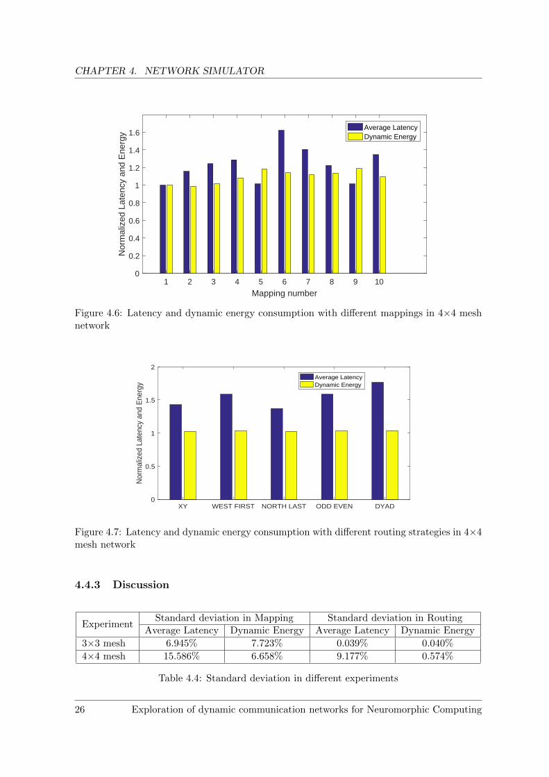
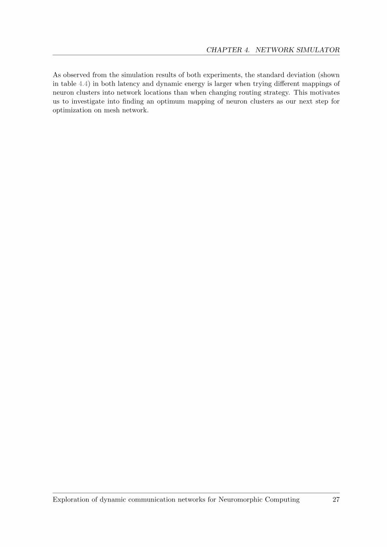
4.6 Latency and dynamic energy consumption with different mappings in 4×4 meshnetwork . . . . . . . . . . . . . . . . . . . . . . . . . . . . . . . . . . . . . . . 26

4.7 Latency and dynamic energy consumption with different routing strategies in4×4 mesh network . . . . . . . . . . . . . . . . . . . . . . . . . . . . . . . . . 26

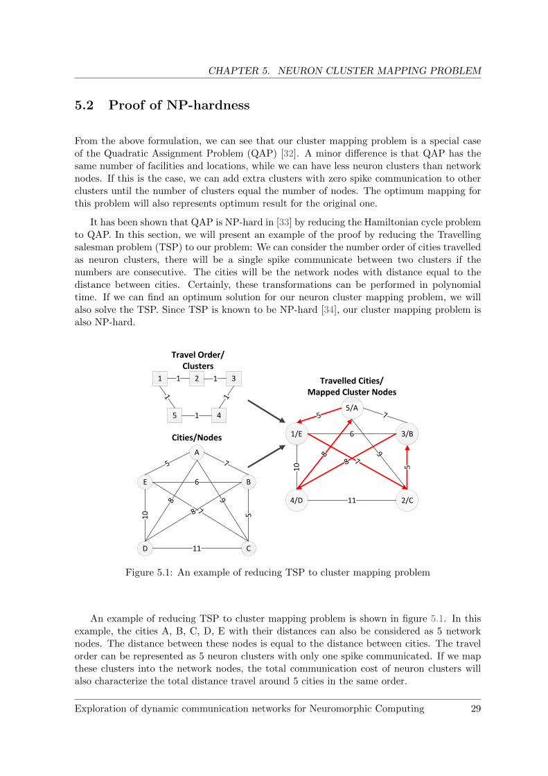
5.1 An example of reducing TSP to cluster mapping problem . . . . . . . . . . . 29

5.2 Comparison of different mapping solutions in 3×3 mesh network . . . . . . . 34




5.6 Average latency and cost function for different mappings in 4×4 mesh network 36

5.7 Dynamic energy and cost function for different mappings in 4×4 mesh network 36

Exploration of dynamic communication networks for Neuromorphic Computing vii

List of Tables

4.1 Simulator preliminary comparison 1 . . . . . . . . . . . . . . . . . . . . . . . 194.2 Simulator preliminary comparison 2 . . . . . . . . . . . . . . . . . . . . . . . 204.3 Simulator detailed comparison . . . . . . . . . . . . . . . . . . . . . . . . . . 214.4 Standard deviation in different experiments . . . . . . . . . . . . . . . . . . . 26

viii Exploration of dynamic communication networks for Neuromorphic Computing

List of Abbreviations

AER Address-Event Representation

BEOL Back End of Line

BFS Breadth First Search

CNN Convolution Neural Network

DPI Differential Pair Integrator

ILP Integer Linear Programming

INI Insitute of Neuroinformatics

MIPS Microprocessor without Interlocked Pipeline Stages

NoC Network-on-Chip

NP Nondeterministic Polynomial Time

QAP Quadratic Assignment Problem

RBM Restricted Boltzmann Machine

RNN Recurrent Neural Network

RTL Register Transfer Level

SNN Spiking Neural Network

STDP Spike Timing Dependent Plasticity

TFT Thin Film Transistor

TLM Transaction Level Modelling

TSP Travelling Salesman Problem

UML Unified Modelling Language

VLSI Vergy Large Scale Integration

WTA Winner-Take-All

Exploration of dynamic communication networks for Neuromorphic Computing ix

Chapter 1

Introduction

1.1 Project background

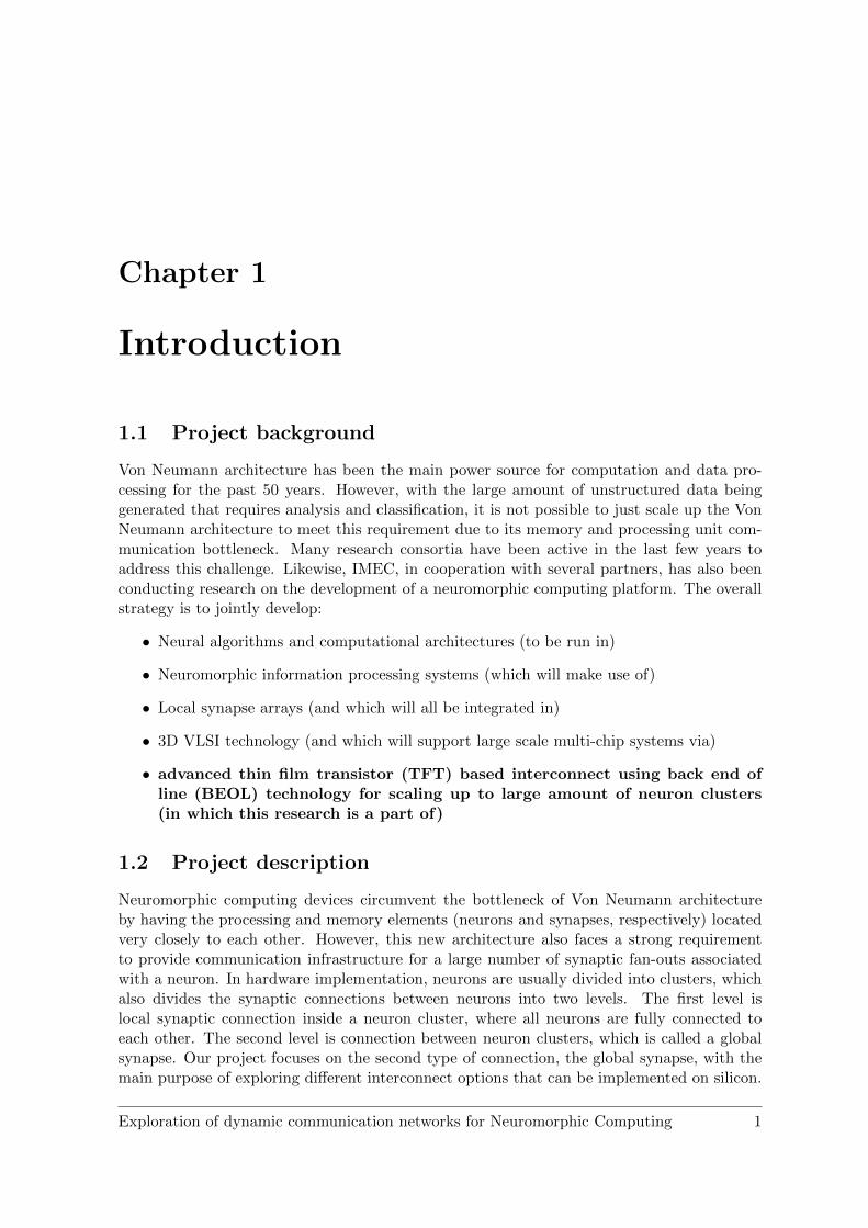
Von Neumann architecture has been the main power source for computation and data pro-cessing for the past 50 years. However, with the large amount of unstructured data beinggenerated that requires analysis and classification, it is not possible to just scale up the VonNeumann architecture to meet this requirement due to its memory and processing unit com-munication bottleneck. Many research consortia have been active in the last few years toaddress this challenge. Likewise, IMEC, in cooperation with several partners, has also beenconducting research on the development of a neuromorphic computing platform. The overallstrategy is to jointly develop:

• Neural algorithms and computational architectures (to be run in)

• Neuromorphic information processing systems (which will make use of)

• Local synapse arrays (and which will all be integrated in)

• 3D VLSI technology (and which will support large scale multi-chip systems via)

• advanced thin film transistor (TFT) based interconnect using back end ofline (BEOL) technology for scaling up to large amount of neuron clusters(in which this research is a part of)

1.2 Project description

Neuromorphic computing devices circumvent the bottleneck of Von Neumann architectureby having the processing and memory elements (neurons and synapses, respectively) locatedvery closely to each other. However, this new architecture also faces a strong requirementto provide communication infrastructure for a large number of synaptic fan-outs associatedwith a neuron. In hardware implementation, neurons are usually divided into clusters, whichalso divides the synaptic connections between neurons into two levels. The first level islocal synaptic connection inside a neuron cluster, where all neurons are fully connected toeach other. The second level is connection between neuron clusters, which is called a globalsynapse. Our project focuses on the second type of connection, the global synapse, with themain purpose of exploring different interconnect options that can be implemented on silicon.

Exploration of dynamic communication networks for Neuromorphic Computing 1

CHAPTER 1. INTRODUCTION

In summary, the project aims at developing a scalable, highly dynamic and flexible com-munication network for neuromorphic clusters that requires low operational power comparableto the human brain.

1.3 Project approach

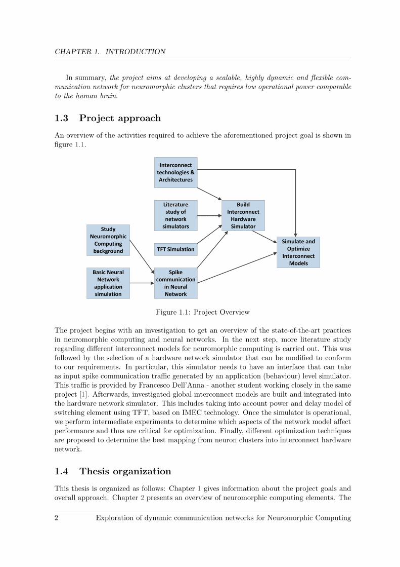
An overview of the activities required to achieve the aforementioned project goal is shown infigure 1.1.

Study Neuromorphic

Computing background

Basic Neural Network

application simulation

Spike communication

in Neural Network

Interconnect technologies & Architectures

Literature study of network

simulators

TFT Simulation

Build Interconnect

Hardware Simulator

Simulate and Optimize

Interconnect Models

Figure 1.1: Project Overview

The project begins with an investigation to get an overview of the state-of-the-art practicesin neuromorphic computing and neural networks. In the next step, more literature studyregarding different interconnect models for neuromorphic computing is carried out. This wasfollowed by the selection of a hardware network simulator that can be modified to conformto our requirements. In particular, this simulator needs to have an interface that can takeas input spike communication traffic generated by an application (behaviour) level simulator.This traffic is provided by Francesco Dell’Anna - another student working closely in the sameproject [1]. Afterwards, investigated global interconnect models are built and integrated intothe hardware network simulator. This includes taking into account power and delay model ofswitching element using TFT, based on IMEC technology. Once the simulator is operational,we perform intermediate experiments to determine which aspects of the network model affectperformance and thus are critical for optimization. Finally, different optimization techniquesare proposed to determine the best mapping from neuron clusters into interconnect hardwarenetwork.

1.4 Thesis organization

This thesis is organized as follows: Chapter 1 gives information about the project goals andoverall approach. Chapter 2 presents an overview of neuromorphic computing elements. The

2 Exploration of dynamic communication networks for Neuromorphic Computing

CHAPTER 1. INTRODUCTION

interconnect models used to represent global synaptic connection between neuron clusters aredescribed in Chapter 3. The literature survey performed to select for a network simulator isdiscussed in Chapter 4. Also in this chapter, the simulator software architecture and its usage,together with some intermediate simulation results are reported. These results lead to theformulation of another research on optimizing mapping neuron clusters into network nodesis presented, which is discussed in Chapter 5. In the same chapter, various algorithms forsolving this problem as well as their simulation results are described and compared. Chapter6 concludes the thesis and lists some interesting topics that can be further explored in futurework.


Chapter 2

Neuromorphic ComputingBackground

2.1 Neuron models

In the brain, neurons are the cells that are responsible for processing and transmitting inform-ation. A typical neuron consist of a body (soma), dendrites (inputs) and an axon (output).The connection between a dendrite and an axon is called a synapse. To mimic the functional-ity of the brain to perform recognition and classification tasks, it is important to understandand build correct behaviour of neuron model. Over the past few decades, many neuron modelshave been developed for performing computation and they can be classified into three maintypes [2]:

• Binary signal neuron;

• Continuous value neuron;

• Spiking neuron.

2.1.1 Binary neuron model

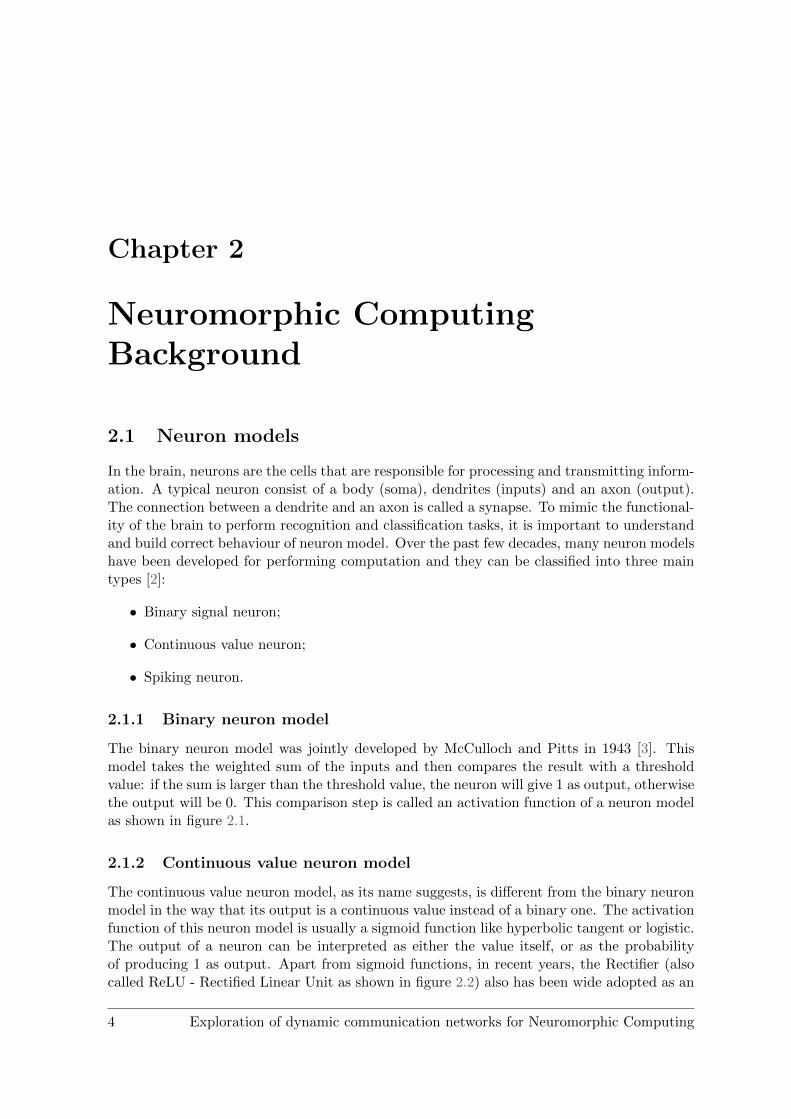
The binary neuron model was jointly developed by McCulloch and Pitts in 1943 [3]. Thismodel takes the weighted sum of the inputs and then compares the result with a thresholdvalue: if the sum is larger than the threshold value, the neuron will give 1 as output, otherwisethe output will be 0. This comparison step is called an activation function of a neuron modelas shown in figure 2.1.

2.1.2 Continuous value neuron model

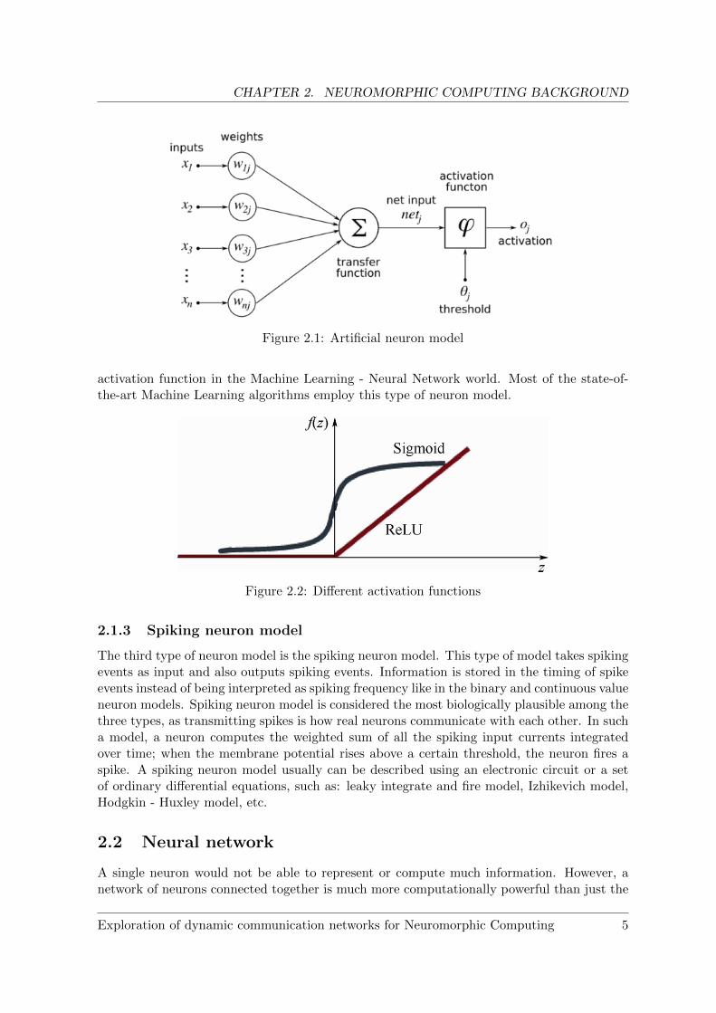
The continuous value neuron model, as its name suggests, is different from the binary neuronmodel in the way that its output is a continuous value instead of a binary one. The activationfunction of this neuron model is usually a sigmoid function like hyperbolic tangent or logistic.The output of a neuron can be interpreted as either the value itself, or as the probabilityof producing 1 as output. Apart from sigmoid functions, in recent years, the Rectifier (alsocalled ReLU - Rectified Linear Unit as shown in figure 2.2) also has been wide adopted as an


CHAPTER 2. NEUROMORPHIC COMPUTING BACKGROUND

Figure 2.1: Artificial neuron model

activation function in the Machine Learning - Neural Network world. Most of the state-of-the-art Machine Learning algorithms employ this type of neuron model.

Figure 2.2: Different activation functions

2.1.3 Spiking neuron model

The third type of neuron model is the spiking neuron model. This type of model takes spikingevents as input and also outputs spiking events. Information is stored in the timing of spikeevents instead of being interpreted as spiking frequency like in the binary and continuous valueneuron models. Spiking neuron model is considered the most biologically plausible among thethree types, as transmitting spikes is how real neurons communicate with each other. In sucha model, a neuron computes the weighted sum of all the spiking input currents integratedover time; when the membrane potential rises above a certain threshold, the neuron fires aspike. A spiking neuron model usually can be described using an electronic circuit or a setof ordinary differential equations, such as: leaky integrate and fire model, Izhikevich model,Hodgkin - Huxley model, etc.

2.2 Neural network

A single neuron would not be able to represent or compute much information. However, anetwork of neurons connected together is much more computationally powerful than just the



mere addition of single neurons. Computation is then usually performed in the context of aneural network. Typically, neurons are organized into layers in such a network.

In the Machine Learning world, many types of neural networks have been developed tosolve different tasks. Usually, the connection setup between layers defines the neural networktype. The networks described in this section are all classified as rate based neural networks,in contrast to the spiking ones.

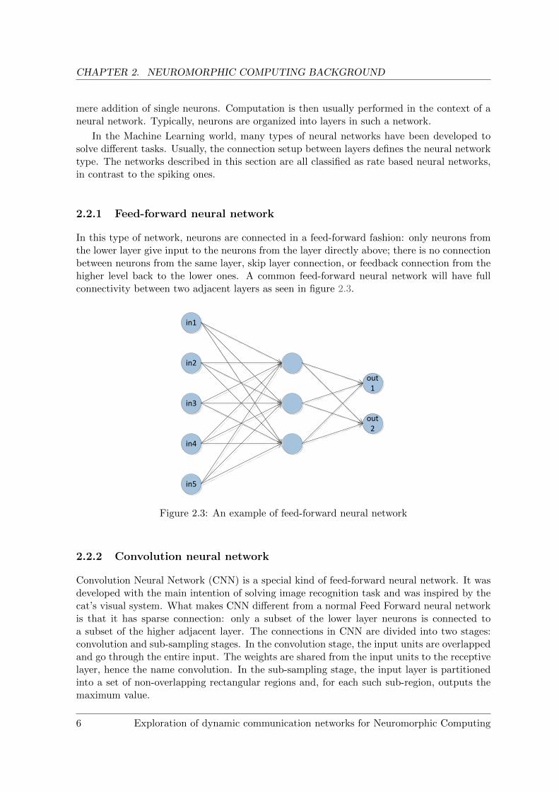
2.2.1 Feed-forward neural network

In this type of network, neurons are connected in a feed-forward fashion: only neurons fromthe lower layer give input to the neurons from the layer directly above; there is no connectionbetween neurons from the same layer, skip layer connection, or feedback connection from thehigher level back to the lower ones. A common feed-forward neural network will have fullconnectivity between two adjacent layers as seen in figure 2.3.

in1

in2

in3

in4

in5

out1

out2

Figure 2.3: An example of feed-forward neural network

2.2.2 Convolution neural network

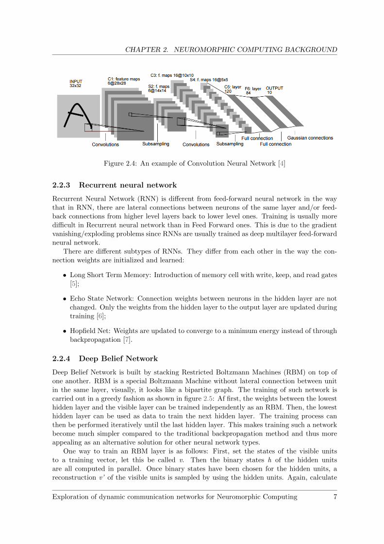
Convolution Neural Network (CNN) is a special kind of feed-forward neural network. It wasdeveloped with the main intention of solving image recognition task and was inspired by thecat’s visual system. What makes CNN different from a normal Feed Forward neural networkis that it has sparse connection: only a subset of the lower layer neurons is connected toa subset of the higher adjacent layer. The connections in CNN are divided into two stages:convolution and sub-sampling stages. In the convolution stage, the input units are overlappedand go through the entire input. The weights are shared from the input units to the receptivelayer, hence the name convolution. In the sub-sampling stage, the input layer is partitionedinto a set of non-overlapping rectangular regions and, for each such sub-region, outputs themaximum value.



Figure 2.4: An example of Convolution Neural Network [4]

2.2.3 Recurrent neural network

Recurrent Neural Network (RNN) is different from feed-forward neural network in the waythat in RNN, there are lateral connections between neurons of the same layer and/or feed-back connections from higher level layers back to lower level ones. Training is usually moredifficult in Recurrent neural network than in Feed Forward ones. This is due to the gradientvanishing/exploding problems since RNNs are usually trained as deep multilayer feed-forwardneural network.

There are different subtypes of RNNs. They differ from each other in the way the con-nection weights are initialized and learned:

• Long Short Term Memory: Introduction of memory cell with write, keep, and read gates[5];

• Echo State Network: Connection weights between neurons in the hidden layer are notchanged. Only the weights from the hidden layer to the output layer are updated duringtraining [6];

• Hopfield Net: Weights are updated to converge to a minimum energy instead of throughbackpropagation [7].

2.2.4 Deep Belief Network

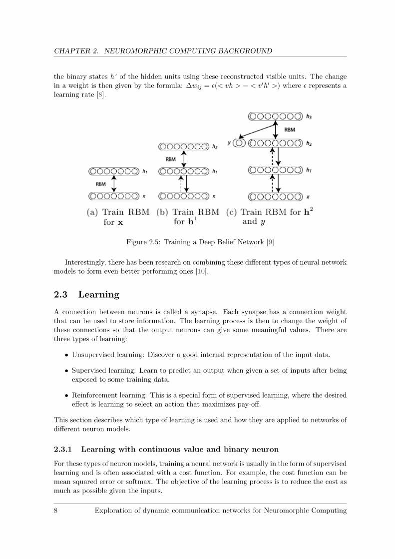
Deep Belief Network is built by stacking Restricted Boltzmann Machines (RBM) on top ofone another. RBM is a special Boltzmann Machine without lateral connection between unitin the same layer, visually, it looks like a bipartite graph. The training of such network iscarried out in a greedy fashion as shown in figure 2.5: Af first, the weights between the lowesthidden layer and the visible layer can be trained independently as an RBM. Then, the lowesthidden layer can be used as data to train the next hidden layer. The training process canthen be performed iteratively until the last hidden layer. This makes training such a networkbecome much simpler compared to the traditional backpropagation method and thus moreappealing as an alternative solution for other neural network types.

One way to train an RBM layer is as follows: First, set the states of the visible unitsto a training vector, let this be called v. Then the binary states h of the hidden unitsare all computed in parallel. Once binary states have been chosen for the hidden units, areconstruction v’ of the visible units is sampled by using the hidden units. Again, calculate



the binary states h’ of the hidden units using these reconstructed visible units. The changein a weight is then given by the formula: ∆wij = ε(< vh > − < v′h′ >) where ε represents alearning rate [8].

Figure 2.5: Training a Deep Belief Network [9]

Interestingly, there has been research on combining these different types of neural networkmodels to form even better performing ones [10].

2.3 Learning

A connection between neurons is called a synapse. Each synapse has a connection weightthat can be used to store information. The learning process is then to change the weight ofthese connections so that the output neurons can give some meaningful values. There arethree types of learning:

• Unsupervised learning: Discover a good internal representation of the input data.

• Supervised learning: Learn to predict an output when given a set of inputs after beingexposed to some training data.

• Reinforcement learning: This is a special form of supervised learning, where the desiredeffect is learning to select an action that maximizes pay-off.

This section describes which type of learning is used and how they are applied to networks ofdifferent neuron models.

2.3.1 Learning with continuous value and binary neuron

For these types of neuron models, training a neural network is usually in the form of supervisedlearning and is often associated with a cost function. For example, the cost function can bemean squared error or softmax. The objective of the learning process is to reduce the cost asmuch as possible given the inputs.



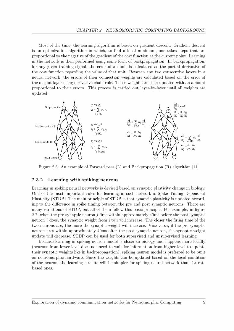
Most of the time, the learning algorithm is based on gradient descent. Gradient descentis an optimization algorithm in which, to find a local minimum, one takes steps that areproportional to the negative of the gradient of the cost function at the current point. Learningin the network is then performed using some form of backpropagation. In backpropagation,for any given training signal, the error of an unit is calculated as the partial derivative ofthe cost function regarding the value of that unit. Between any two consecutive layers in aneural network, the errors of their connection weights are calculated based on the error ofthe output layer using derivative chain rule. These weights are then updated with an amountproportional to their errors. This process is carried out layer-by-layer until all weights areupdated.

Figure 2.6: An example of Forward pass (L) and Backpropagation (R) algorithm [11]

2.3.2 Learning with spiking neurons

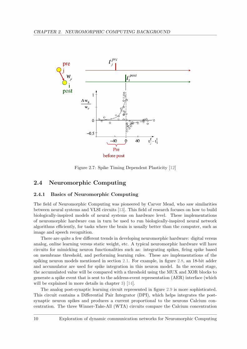
Learning in spiking neural networks is devised based on synaptic plasticity change in biology.One of the most important rules for learning in such network is Spike Timing DependentPlasticity (STDP). The main principle of STDP is that synaptic plasticity is updated accord-ing to the difference in spike timing between the pre and post synaptic neurons. There aremany variations of STDP, but all of them follow this basic principle. For example, in figure2.7, when the pre-synaptic neuron j fires within approximately 40ms before the post-synapticneuron i does, the synaptic weight from j to i will increase. The closer the firing time of thetwo neurons are, the more the synaptic weight will increase. Vice versa, if the pre-synapticneuron fires within approximately 40ms after the post-synaptic neuron, the synaptic weightupdate will decrease. STDP can be used for both supervised and unsupervised learning.

Because learning in spiking neuron model is closer to biology and happens more locally(neurons from lower level does not need to wait for information from higher level to updatetheir synaptic weights like in backpropagation), spiking neuron model is preferred to be builton neuromorphic hardware. Since the weights can be updated based on the local conditionof the neuron, the learning circuits will be simpler for spiking neural network than for ratebased ones.



Figure 2.7: Spike Timing Dependent Plasticity [12]

2.4 Neuromorphic Computing

2.4.1 Basics of Neuromorphic Computing

The field of Neuromorphic Computing was pioneered by Carver Mead, who saw similaritiesbetween neural systems and VLSI circuits [13]. This field of research focuses on how to buildbiologically-inspired models of neural systems on hardware level. These implementationsof neuromorphic hardware can in turn be used to run biologically-inspired neural networkalgorithms efficiently, for tasks where the brain is usually better than the computer, such asimage and speech recognition.

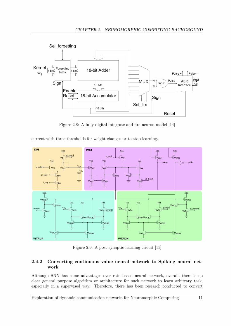
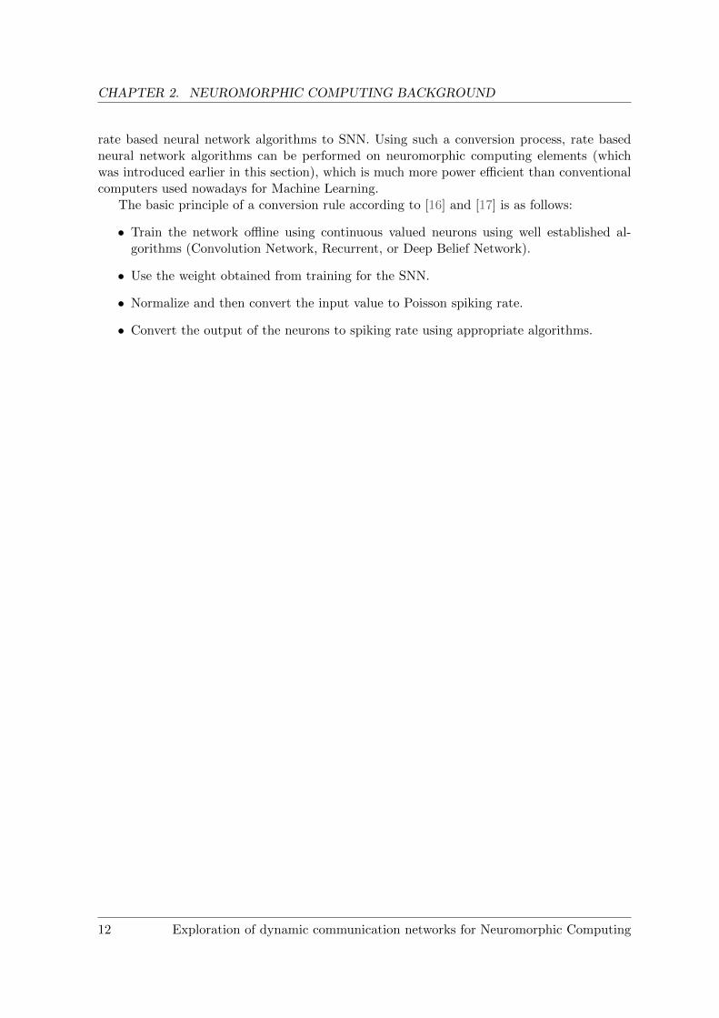
There are quite a few different trends in developing neuromorphic hardware: digital versusanalog, online learning versus static weight, etc. A typical neuromorphic hardware will havecircuits for mimicking neuron functionalities such as: integrating spikes, firing spike basedon membrane threshold, and performing learning rules. These are implementations of thespiking neuron models mentioned in section 2.1. For example, in figure 2.8, an 18-bit adderand accumulator are used for spike integration in this neuron model. In the second stage,the accumulated value will be compared with a threshold using the MUX and XOR blocks togenerate a spike event that is sent to the address-event representation (AER) interface (whichwill be explained in more details in chapter 3) [14].

The analog post-synaptic learning circuit represented in figure 2.9 is more sophisticated.This circuit contains a Differential Pair Integrator (DPI), which helps integrates the post-synaptic neuron spikes and produces a current proportional to the neurons Calcium con-centration. The three Winner-Take-All (WTA) circuits compare the Calcium concentration



Figure 2.8: A fully digital integrate and fire neuron model [14]

current with three thresholds for weight changes or to stop learning.

Figure 2.9: A post-synaptic learning circuit [15]

2.4.2 Converting continuous value neural network to Spiking neural net-work

Although SNN has some advantages over rate based neural network, overall, there is noclear general purpose algorithm or architecture for such network to learn arbitrary task,especially in a supervised way. Therefore, there has been research conducted to convert



rate based neural network algorithms to SNN. Using such a conversion process, rate basedneural network algorithms can be performed on neuromorphic computing elements (whichwas introduced earlier in this section), which is much more power efficient than conventionalcomputers used nowadays for Machine Learning.

The basic principle of a conversion rule according to [16] and [17] is as follows:

• Train the network offline using continuous valued neurons using well established al-gorithms (Convolution Network, Recurrent, or Deep Belief Network).

• Use the weight obtained from training for the SNN.

• Normalize and then convert the input value to Poisson spiking rate.

• Convert the output of the neurons to spiking rate using appropriate algorithms.


Chapter 3

Scalable NeuromorphicInterconnects

3.1 Communication in neuromorphic computing

A challenging task in building neuromorphic computing hardware is trying to accommodatethe number of synaptic connections within the human brain: a typical neuron has approxim-ately 5000 to 10000 synaptic connections. One of the reasons that this is difficult to implementon hardware is brain synapses are connected in 3D while the VLSI approach usually can onlyprovide connections in 2D. Additionally, area overhead and energy consumption for wiringand I/Os will be very large to implement those connections physically, especially when thenumber of neurons approach hundred millions or even billions like in the human brain.

One way to reduce the complexity of implementing a large number of connections inhardware is to utilize time multiplexing. This is sensible to do as spiking actions in the brainhappens in time range of milliseconds and the VLSI communication hardware is 3 to 6 orderof magnitude fasters than that.

The de facto way to transmit spiking event in a large neuromorphic systems is by address-event representation (AER) protocol. Using this protocol, spike events are broadcast digitallywith only the address of the neuron that emits the spike [18]. Time represents itself in sucha configuration. Usually, the width and amplitude of the spike are not transmitted as theydo not contain useful information [19]. However, in the case that such information is needed,the AER protocol can be extended to include the required data.

Another way to reduce the number of connections is to try to identify the structure ofthe neural network and remove the connections that are not necessary. In brain networks, ithas been found that neurons are connected in a small-world structure: neurons that are closetogether group into clusters and are connected in a (near) clique fashion, between clustersthere are long connections that greatly reduce the path length between neurons from differentclusters [20]. This is reflected in recent developments in neuromorphic computing: artificialneurons are grouped into clusters where they are fully connected (local connectivity), andin between clusters there are interconnects, where spiking communication happens less fre-quently (global connectivity).

Both the cxQuad chip [21] developed by Insitute of Neuroinformatics (INI) in Zurich andthe TrueNorth chip developed by IBM utilize aforementioned approaches for reducing com-munication complexity. The cxQuad chip implements a two-stage Network-on-Chip (NoC)


CHAPTER 3. SCALABLE NEUROMORPHIC INTERCONNECTS

for the long interconnect to reduce memory requirement while still being able to have someflexibility for the network to adapt [22]. The IBM’s TrueNorth chip, on the other hand, im-plements a time multiplexed mesh based network for the long interconnect [23]. These twoapproaches, together with the dynamically controlled segmented bus network developed inIMEC Leuven, will form the main interconnect models for comparison in this project.

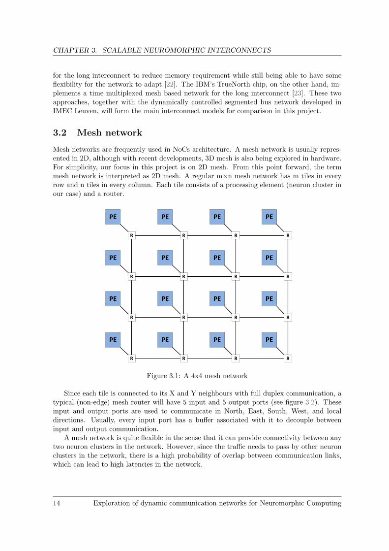
3.2 Mesh network

Mesh networks are frequently used in NoCs architecture. A mesh network is usually repres-ented in 2D, although with recent developments, 3D mesh is also being explored in hardware.For simplicity, our focus in this project is on 2D mesh. From this point forward, the termmesh network is interpreted as 2D mesh. A regular m×n mesh network has m tiles in everyrow and n tiles in every column. Each tile consists of a processing element (neuron cluster inour case) and a router.

PE

R

PE

R

PE

R

PE

R

PE

R

PE

R

PE

R

PE

R

PE

R

PE

R

PE

R

PE

R

PE

R

PE

R

PE

R

PE

R

Figure 3.1: A 4x4 mesh network

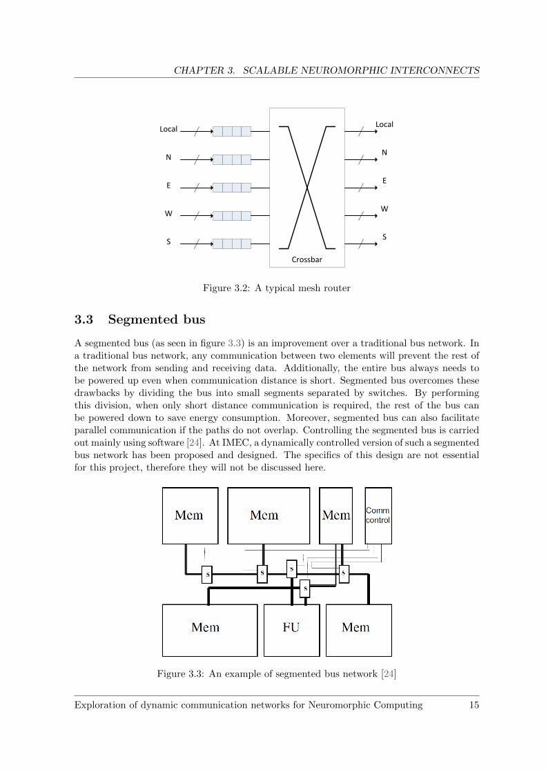
Since each tile is connected to its X and Y neighbours with full duplex communication, atypical (non-edge) mesh router will have 5 input and 5 output ports (see figure 3.2). Theseinput and output ports are used to communicate in North, East, South, West, and localdirections. Usually, every input port has a buffer associated with it to decouple betweeninput and output communication.

A mesh network is quite flexible in the sense that it can provide connectivity between anytwo neuron clusters in the network. However, since the traffic needs to pass by other neuronclusters in the network, there is a high probability of overlap between communication links,which can lead to high latencies in the network.



Local

N

S

W

E

N

S

W

E

Local

Crossbar

Figure 3.2: A typical mesh router

3.3 Segmented bus

A segmented bus (as seen in figure 3.3) is an improvement over a traditional bus network. Ina traditional bus network, any communication between two elements will prevent the rest ofthe network from sending and receiving data. Additionally, the entire bus always needs tobe powered up even when communication distance is short. Segmented bus overcomes thesedrawbacks by dividing the bus into small segments separated by switches. By performingthis division, when only short distance communication is required, the rest of the bus canbe powered down to save energy consumption. Moreover, segmented bus can also facilitateparallel communication if the paths do not overlap. Controlling the segmented bus is carriedout mainly using software [24]. At IMEC, a dynamically controlled version of such a segmentedbus network has been proposed and designed. The specifics of this design are not essentialfor this project, therefore they will not be discussed here.

Figure 3.3: An example of segmented bus network [24]



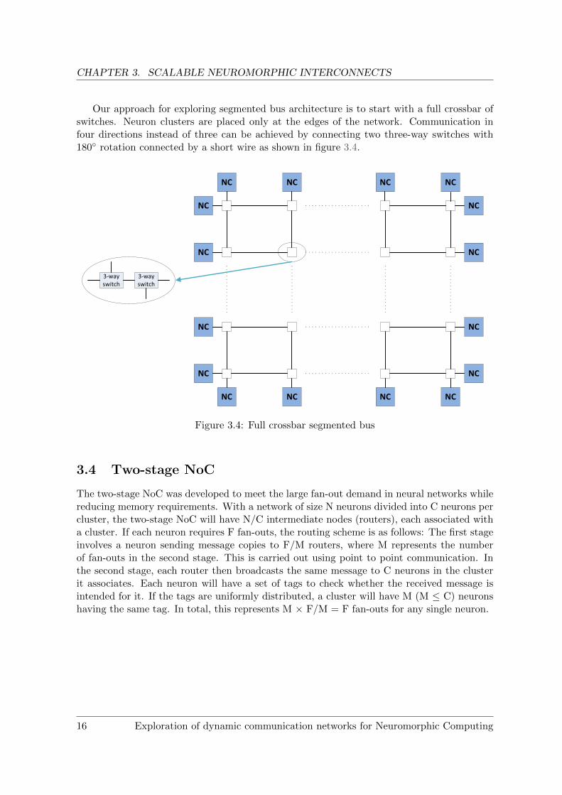
Our approach for exploring segmented bus architecture is to start with a full crossbar ofswitches. Neuron clusters are placed only at the edges of the network. Communication infour directions instead of three can be achieved by connecting two three-way switches with180◦ rotation connected by a short wire as shown in figure 3.4.

NC

NC NC

NC

NC

NC

NC NC NC NC

NC

NC

NC

NC

NC NC

3-way switch

3-way switch

Figure 3.4: Full crossbar segmented bus

3.4 Two-stage NoC

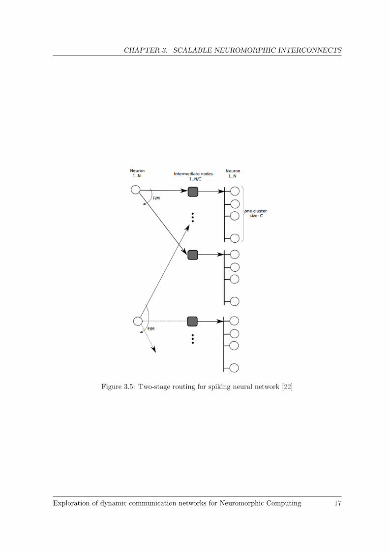
The two-stage NoC was developed to meet the large fan-out demand in neural networks whilereducing memory requirements. With a network of size N neurons divided into C neurons percluster, the two-stage NoC will have N/C intermediate nodes (routers), each associated witha cluster. If each neuron requires F fan-outs, the routing scheme is as follows: The first stageinvolves a neuron sending message copies to F/M routers, where M represents the numberof fan-outs in the second stage. This is carried out using point to point communication. Inthe second stage, each router then broadcasts the same message to C neurons in the clusterit associates. Each neuron will have a set of tags to check whether the received message isintended for it. If the tags are uniformly distributed, a cluster will have M (M ≤ C) neuronshaving the same tag. In total, this represents M × F/M = F fan-outs for any single neuron.



Figure 3.5: Two-stage routing for spiking neural network [22]


Chapter 4

Network Simulator

4.1 Discrete-Event and Cycle-Accurate simulators

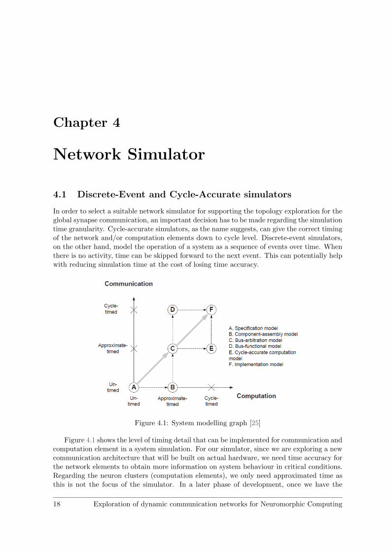
In order to select a suitable network simulator for supporting the topology exploration for theglobal synapse communication, an important decision has to be made regarding the simulationtime granularity. Cycle-accurate simulators, as the name suggests, can give the correct timingof the network and/or computation elements down to cycle level. Discrete-event simulators,on the other hand, model the operation of a system as a sequence of events over time. Whenthere is no activity, time can be skipped forward to the next event. This can potentially helpwith reducing simulation time at the cost of losing time accuracy.

Figure 4.1: System modelling graph [25]

Figure 4.1 shows the level of timing detail that can be implemented for communication andcomputation element in a system simulation. For our simulator, since we are exploring a newcommunication architecture that will be built on actual hardware, we need time accuracy forthe network elements to obtain more information on system behaviour in critical conditions.Regarding the neuron clusters (computation elements), we only need approximated time asthis is not the focus of the simulator. In a later phase of development, once we have the


CHAPTER 4. NETWORK SIMULATOR

network type chosen, the simulator can be extended to have more relaxed timing accuracyon network elements for faster simulation on large networks (up to 10000 neuron clusters).Thus, we position our simulator on points C and D according to figure 4.1.

4.2 Simulator choices

It is possible to develop our own hardware network simulator from scratch. However, thatwould mean spending a lot of time reinventing the wheel for more simple features that arealready available in a well-developed network simulator. Hence, we choose to find a suitablesimulator and then modify it according to our requirements.

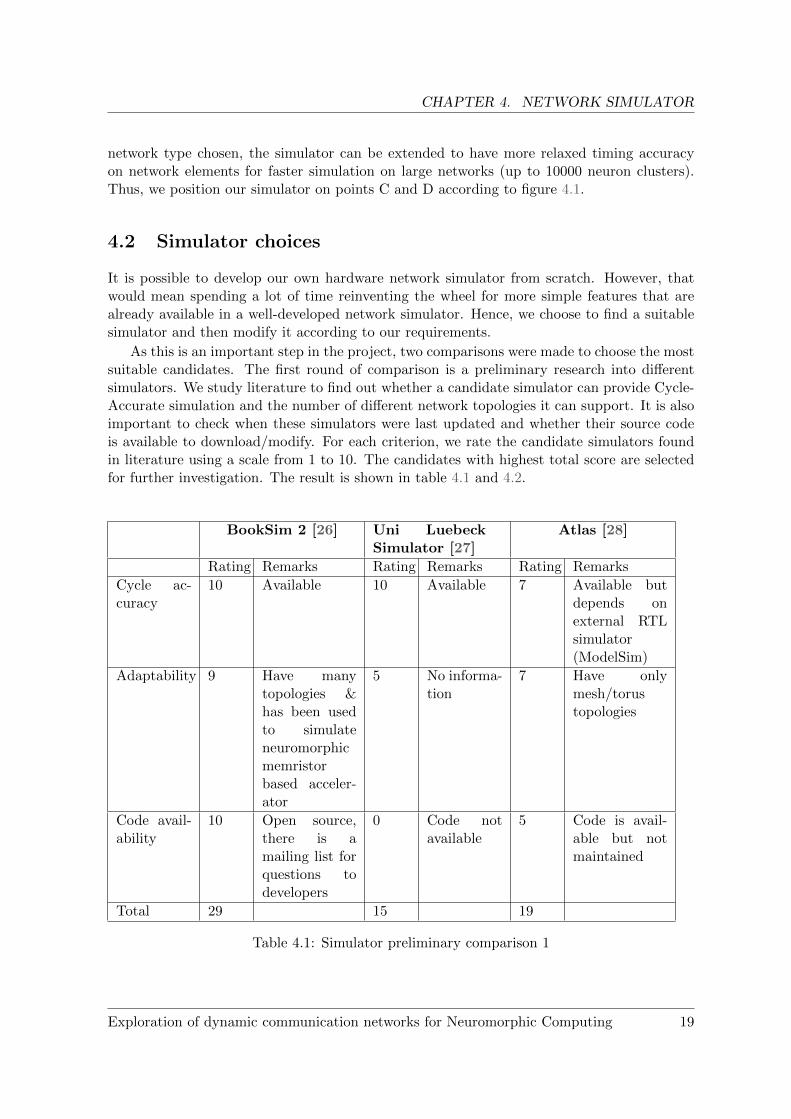
As this is an important step in the project, two comparisons were made to choose the mostsuitable candidates. The first round of comparison is a preliminary research into differentsimulators. We study literature to find out whether a candidate simulator can provide Cycle-Accurate simulation and the number of different network topologies it can support. It is alsoimportant to check when these simulators were last updated and whether their source codeis available to download/modify. For each criterion, we rate the candidate simulators foundin literature using a scale from 1 to 10. The candidates with highest total score are selectedfor further investigation. The result is shown in table 4.1 and 4.2.

BookSim 2 [26] Uni LuebeckSimulator [27]

Atlas [28]

Rating Remarks Rating Remarks Rating Remarks

Cycle ac-curacy

10 Available 10 Available 7 Available butdepends onexternal RTLsimulator(ModelSim)

Adaptability 9 Have manytopologies &has been usedto simulateneuromorphicmemristorbased acceler-ator

5 No informa-tion

7 Have onlymesh/torustopologies

Code avail-ability

10 Open source,there is amailing list forquestions todevelopers

0 Code notavailable

5 Code is avail-able but notmaintained

Total 29 15 19

Table 4.1: Simulator preliminary comparison 1



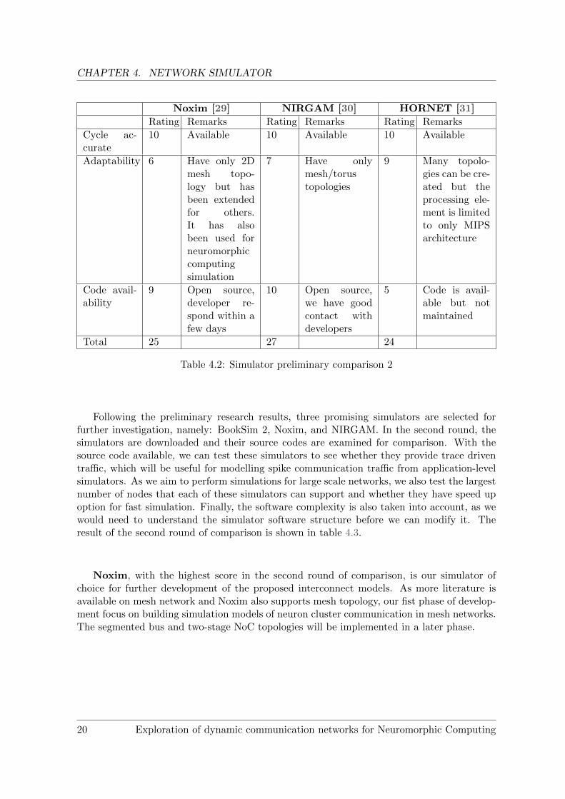
Noxim [29] NIRGAM [30] HORNET [31]


Cycle ac-curate

10 Available 10 Available 10 Available

Adaptability 6 Have only 2Dmesh topo-logy but hasbeen extendedfor others.It has alsobeen used forneuromorphiccomputingsimulation

7 Have onlymesh/torustopologies

9 Many topolo-gies can be cre-ated but theprocessing ele-ment is limitedto only MIPSarchitecture

Code avail-ability

9 Open source,developer re-spond within afew days

10 Open source,we have goodcontact withdevelopers

5 Code is avail-able but notmaintained

Total 25 27 24

Table 4.2: Simulator preliminary comparison 2

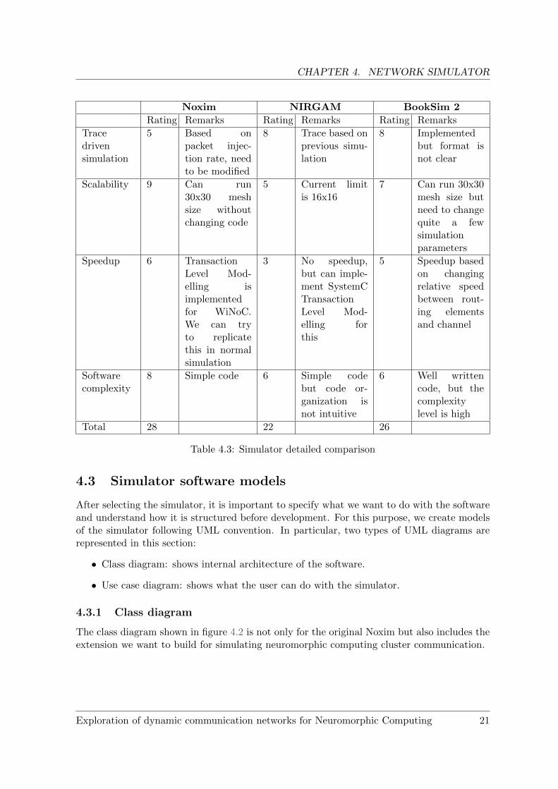
Following the preliminary research results, three promising simulators are selected forfurther investigation, namely: BookSim 2, Noxim, and NIRGAM. In the second round, thesimulators are downloaded and their source codes are examined for comparison. With thesource code available, we can test these simulators to see whether they provide trace driventraffic, which will be useful for modelling spike communication traffic from application-levelsimulators. As we aim to perform simulations for large scale networks, we also test the largestnumber of nodes that each of these simulators can support and whether they have speed upoption for fast simulation. Finally, the software complexity is also taken into account, as wewould need to understand the simulator software structure before we can modify it. Theresult of the second round of comparison is shown in table 4.3.

Noxim, with the highest score in the second round of comparison, is our simulator ofchoice for further development of the proposed interconnect models. As more literature isavailable on mesh network and Noxim also supports mesh topology, our fist phase of develop-ment focus on building simulation models of neuron cluster communication in mesh networks.The segmented bus and two-stage NoC topologies will be implemented in a later phase.



Noxim NIRGAM BookSim 2


Tracedrivensimulation

5 Based onpacket injec-tion rate, needto be modified

8 Trace based onprevious simu-lation

8 Implementedbut format isnot clear

Scalability 9 Can run30x30 meshsize withoutchanging code

5 Current limitis 16x16

7 Can run 30x30mesh size butneed to changequite a fewsimulationparameters

Speedup 6 TransactionLevel Mod-elling isimplementedfor WiNoC.We can tryto replicatethis in normalsimulation

3 No speedup,but can imple-ment SystemCTransactionLevel Mod-elling forthis

5 Speedup basedon changingrelative speedbetween rout-ing elementsand channel

Softwarecomplexity

8 Simple code 6 Simple codebut code or-ganization isnot intuitive

6 Well writtencode, but thecomplexitylevel is high

Total 28 22 26

Table 4.3: Simulator detailed comparison

4.3 Simulator software models

After selecting the simulator, it is important to specify what we want to do with the softwareand understand how it is structured before development. For this purpose, we create modelsof the simulator following UML convention. In particular, two types of UML diagrams arerepresented in this section:

• Class diagram: shows internal architecture of the software.

• Use case diagram: shows what the user can do with the simulator.

4.3.1 Class diagram

The class diagram shown in figure 4.2 is not only for the original Noxim but also includes theextension we want to build for simulating neuromorphic computing cluster communication.



Fig

ure

4.2:

Sim

ula

tor

clas

sd

iagr

am



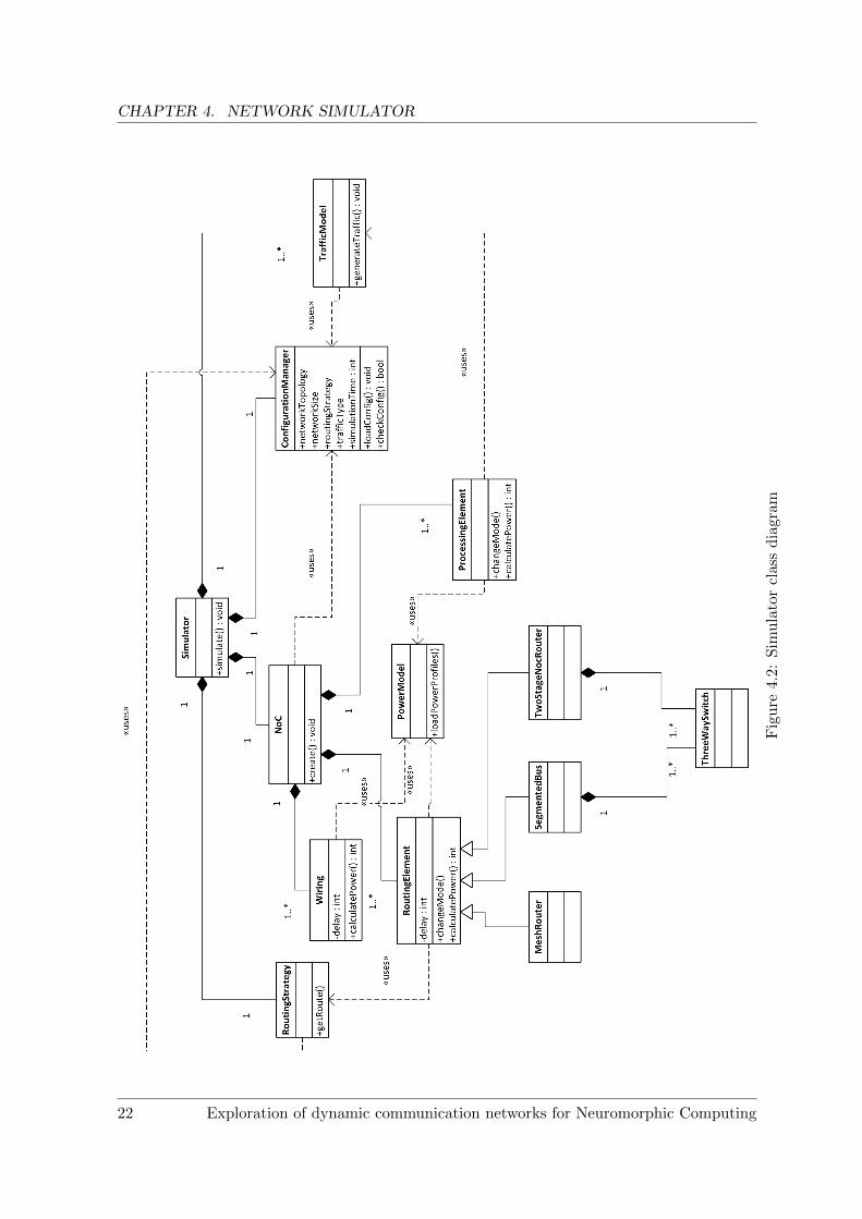
Due to size limitation, the following details need to be omitted from the class diagram:

• Routing Strategy is the generalization class of the following routing strategies:

– Dyad;

– Negative first;

– North last;

– Odd even;

– Table based;

– West first;

– XY.

• Traffic Model is able to generate traffic based on the following traffic models:

– Random;

– Transpose matrix;

– Bit-reversal;

– Butterfly;

– Shuffle;

– Table based.

• Configuration Manager loads input parameters from a file and passes the required in-formation to other classes. The input parameters include, but are not limited to:

– Network topology;

– Network size;

– Traffic type;

– Routing strategy;

– Simulation time.

• Power Model loads power (and potentially area) profiles from a file and provides power(and area) calculation for other classes like Routing Element or Processing Element.

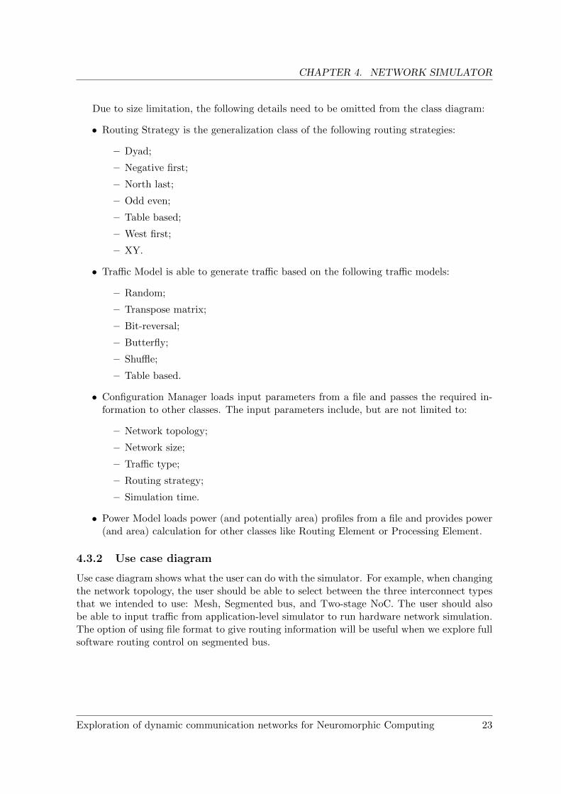
4.3.2 Use case diagram

Use case diagram shows what the user can do with the simulator. For example, when changingthe network topology, the user should be able to select between the three interconnect typesthat we intended to use: Mesh, Segmented bus, and Two-stage NoC. The user should alsobe able to input traffic from application-level simulator to run hardware network simulation.The option of using file format to give routing information will be useful when we explore fullsoftware routing control on segmented bus.



User

Change networktopology

Change network size

Input routingcontrol using file

Change routingstrategy

Input traffic type

Start/Stopsimulation

Input simulationparameters

Input trafficusing file

Change simulationmode

<<extends>>

<<extends>>

<<include>>

<<include>>

<<include>>

<<include>>

Figure 4.3: Simulator use case diagram

4.4 Intermediate simulation results

After implementing mesh network in the simulator, we perform some experiments to verifythat the simulator is working as expected. For example, to test the scalability of the simulator,we try to simulate a large network. We succeeded in performing simulations for mesh networkup to 10000 (100×100) nodes. This takes 1 hour and 15 minutes to simulate 30ms of spiketraffic, with 2.2 million spiking events in total.

Furthermore, we need to identify performance issues for architectural optimization in meshnetwork. Since we are looking for low power implementations, our main focus for comparisonin these experiments is energy consumption. Another aspect worth investigating is latency,as high latency of spike communication can have a potential effect on STDP learning andlead to degradation of the neural network application.

4.4.1 3×3 mesh experiment

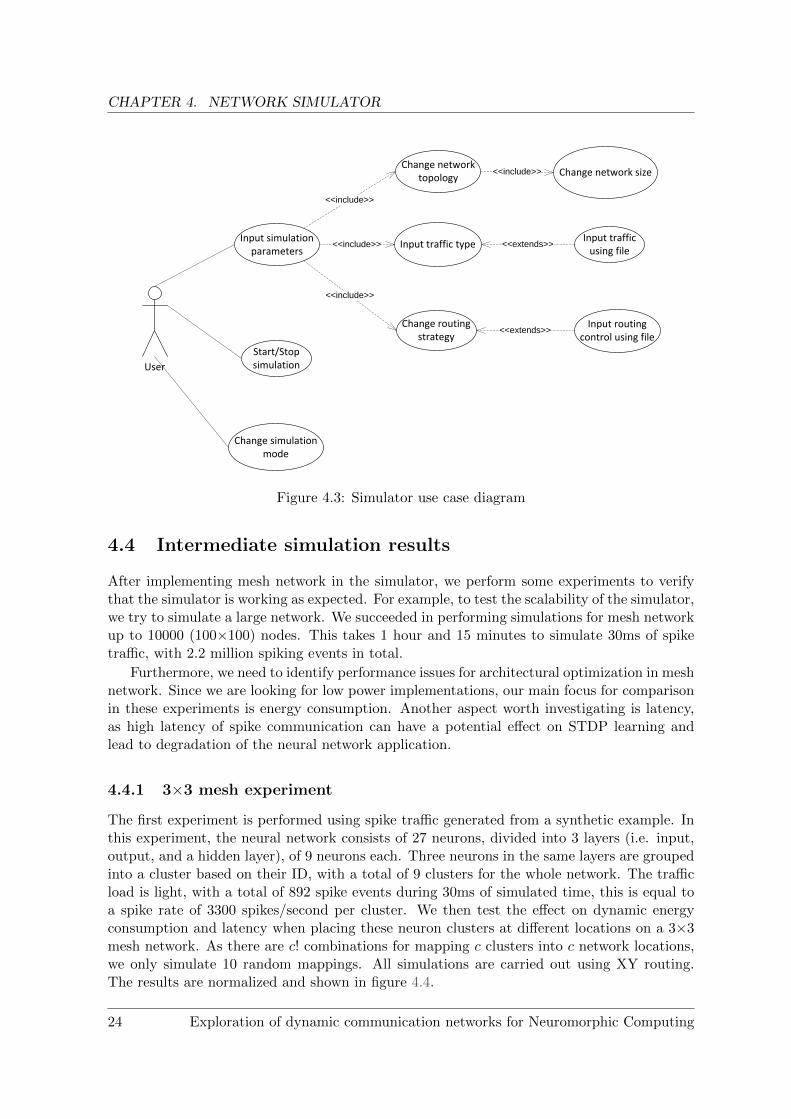
The first experiment is performed using spike traffic generated from a synthetic example. Inthis experiment, the neural network consists of 27 neurons, divided into 3 layers (i.e. input,output, and a hidden layer), of 9 neurons each. Three neurons in the same layers are groupedinto a cluster based on their ID, with a total of 9 clusters for the whole network. The trafficload is light, with a total of 892 spike events during 30ms of simulated time, this is equal toa spike rate of 3300 spikes/second per cluster. We then test the effect on dynamic energyconsumption and latency when placing these neuron clusters at different locations on a 3×3mesh network. As there are c! combinations for mapping c clusters into c network locations,we only simulate 10 random mappings. All simulations are carried out using XY routing.The results are normalized and shown in figure 4.4.



1 2 3 4 5 6 7 8 9 10

Mapping number

0

0.2

0.4

0.6

0.8

1

1.2

1.4

Nor

mal

ized

Lat

ency

and

Ene

rgy

Average LatencyDynamic Energy

Figure 4.4: Latency and dynamic energy consumption with different mappings in 3×3 meshnetwork

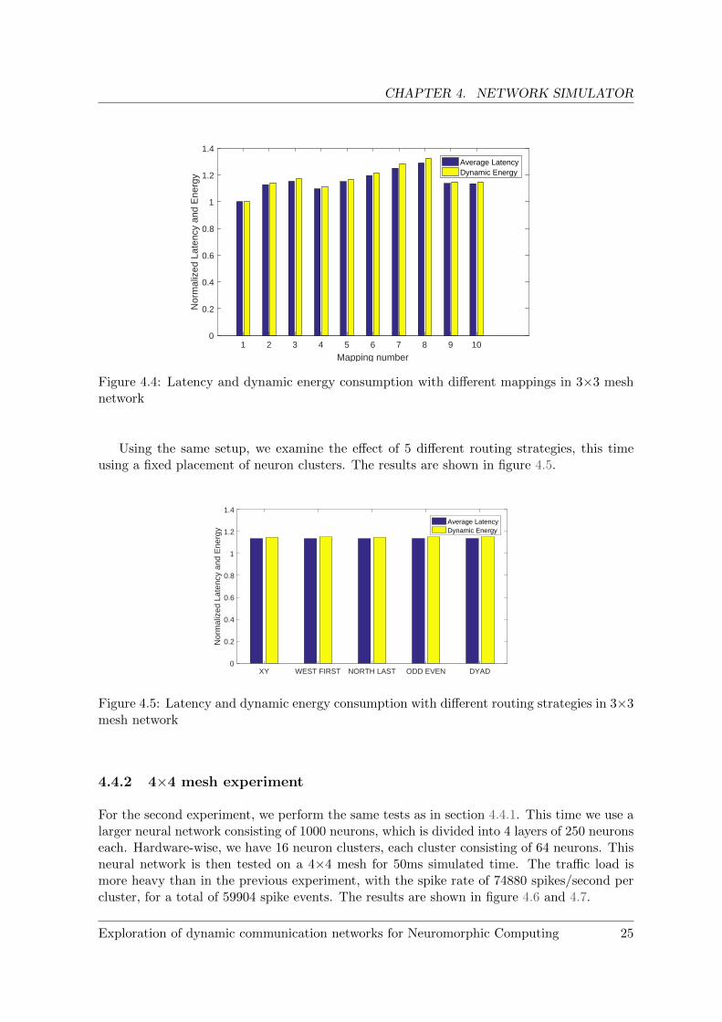
Using the same setup, we examine the effect of 5 different routing strategies, this timeusing a fixed placement of neuron clusters. The results are shown in figure 4.5.

XY WEST FIRST NORTH LAST ODD EVEN DYAD0

0.2

0.4

0.6

0.8

1

1.2

1.4

Nor

mal

ized

Lat

ency

and

Ene

rgy


Figure 4.5: Latency and dynamic energy consumption with different routing strategies in 3×3mesh network

4.4.2 4×4 mesh experiment

For the second experiment, we perform the same tests as in section 4.4.1. This time we use alarger neural network consisting of 1000 neurons, which is divided into 4 layers of 250 neuronseach. Hardware-wise, we have 16 neuron clusters, each cluster consisting of 64 neurons. Thisneural network is then tested on a 4×4 mesh for 50ms simulated time. The traffic load ismore heavy than in the previous experiment, with the spike rate of 74880 spikes/second percluster, for a total of 59904 spike events. The results are shown in figure 4.6 and 4.7.



1 2 3 4 5 6 7 8 9 10

Mapping number

0

0.2

0.4

0.6

0.8

1

1.2

1.4

1.6

Nor

mal

ized

Lat

ency

and

Ene

rgy


Figure 4.6: Latency and dynamic energy consumption with different mappings in 4×4 meshnetwork

XY WEST FIRST NORTH LAST ODD EVEN DYAD0

0.5

1

1.5

2

Nor

mal

ized

Lat

ency

and

Ene

rgy


Figure 4.7: Latency and dynamic energy consumption with different routing strategies in 4×4mesh network

4.4.3 Discussion

ExperimentStandard deviation in Mapping Standard deviation in Routing

Average Latency Dynamic Energy Average Latency Dynamic Energy

3×3 mesh 6.945% 7.723% 0.039% 0.040%

4×4 mesh 15.586% 6.658% 9.177% 0.574%

Table 4.4: Standard deviation in different experiments



As observed from the simulation results of both experiments, the standard deviation (shownin table 4.4) in both latency and dynamic energy is larger when trying different mappings ofneuron clusters into network locations than when changing routing strategy. This motivatesus to investigate into finding an optimum mapping of neuron clusters as our next step foroptimization on mesh network.


Chapter 5

Neuron Cluster Mapping Problem

As observed in the simulation results of chapter 4, we can improve on energy efficiency ofcommunication by taking care of where the neuron clusters are located and how often theycommunicate.

In principle, the optimization for global synapse communication when mapping a neuralnetwork into hardware can also be carried out while grouping neurons into clusters. This ispossible if we group neurons that often communicate with each other in the same cluster,which keeps the communication local and thus reduces the cost. Another strategy would begrouping neurons that are connected to the same axons in one cluster. This way, since a spikeis broadcast to all neurons inside a cluster, there will be less duplication of spike messages oninter-cluster communication level.

The whole problem of mapping a neural network into hardware, however, is a very largesearch space. Thus we divide this optimization work into two steps: The first step is mappingneurons into neuron clusters of similar size; the second step is to map these neuron clustersinto actual network nodes. The first step is carried out by Thibaut Marty - another studentworking on the same project. In this chapter, our work is focused on the second step.

First, we formally define the problem of mapping neuron clusters to network nodes. Wethen motive the need to apply heuristics to this problem. Finally, different algorithms areproposed to solve this optimization problem approximately.

5.1 Problem formulation

The optimization problem can be stated as mapping a set of neuron clusters to a set ofnetwork nodes where one cluster can be mapped to one and only one node. For each pair ofclusters, there is a number of spikes that communicate between them, while between each pairof network nodes there is a distance specified. The objective of the problem is to minimizethe sum of spikes that need to travel through the distance between the nodes.

More formally, we have c neuron clusters that need to be mapped to n network nodes(c ≤ n). sij represents the number of spikes communicated from cluster i to cluster j, forall i, j ∈ C = {1, 2, .., c}. dxy represents the distance between node x and node y, for allx, y ∈ N = {1, 2, .., n}. The function φ : C → N defines a mapping from clusters to nodes.The objective is then to find a mapping that minimizes the following cost function:∑

i∈C

∑j∈C

sijdφ(i)φ(j) (5.1)


CHAPTER 5. NEURON CLUSTER MAPPING PROBLEM

5.2 Proof of NP-hardness

From the above formulation, we can see that our cluster mapping problem is a special caseof the Quadratic Assignment Problem (QAP) [32]. A minor difference is that QAP has thesame number of facilities and locations, while we can have less neuron clusters than networknodes. If this is the case, we can add extra clusters with zero spike communication to otherclusters until the number of clusters equal the number of nodes. The optimum mapping forthis problem will also represents optimum result for the original one.

It has been shown that QAP is NP-hard in [33] by reducing the Hamiltonian cycle problemto QAP. In this section, we will present an example of the proof by reducing the Travellingsalesman problem (TSP) to our problem: We can consider the number order of cities travelledas neuron clusters, there will be a single spike communicate between two clusters if thenumbers are consecutive. The cities will be the network nodes with distance equal to thedistance between cities. Certainly, these transformations can be performed in polynomialtime. If we can find an optimum solution for our neuron cluster mapping problem, we willalso solve the TSP. Since TSP is known to be NP-hard [34], our cluster mapping problem isalso NP-hard.

A

E B

D C11

5

6

7

9

5 7

8

10

1 2 3

5 4

1 11

1

1

Travel Order/Clusters

Cities/Nodes

5/A

1/E 3/B

4/D 2/C11

5

6

7

9

5 7

8

10

Travelled Cities/Mapped Cluster Nodes

8

8

Figure 5.1: An example of reducing TSP to cluster mapping problem

An example of reducing TSP to cluster mapping problem is shown in figure 5.1. In thisexample, the cities A, B, C, D, E with their distances can also be considered as 5 networknodes. The distance between these nodes is equal to the distance between cities. The travelorder can be represented as 5 neuron clusters with only one spike communicated. If we mapthese clusters into the network nodes, the total communication cost of neuron clusters willalso characterize the total distance travel around 5 cities in the same order.



5.3 Solution algorithms

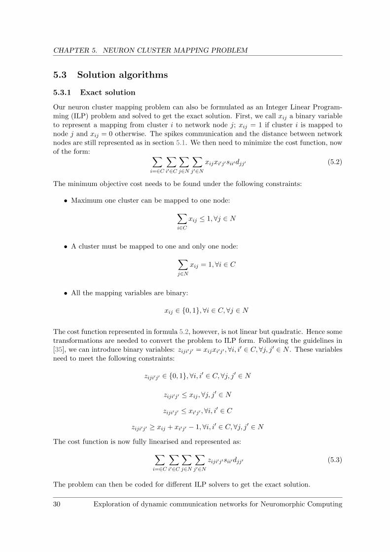
5.3.1 Exact solution

Our neuron cluster mapping problem can also be formulated as an Integer Linear Program-ming (ILP) problem and solved to get the exact solution. First, we call xij a binary variableto represent a mapping from cluster i to network node j; xij = 1 if cluster i is mapped tonode j and xij = 0 otherwise. The spikes communication and the distance between networknodes are still represented as in section 5.1. We then need to minimize the cost function, nowof the form: ∑

i=∈C

∑i′∈C

∑j∈N

∑j′∈N

xijxi′j′sii′djj′ (5.2)

The minimum objective cost needs to be found under the following constraints:

• Maximum one cluster can be mapped to one node:∑i∈C

xij ≤ 1,∀j ∈ N

• A cluster must be mapped to one and only one node:∑j∈N

xij = 1,∀i ∈ C

• All the mapping variables are binary:

xij ∈ {0, 1},∀i ∈ C,∀j ∈ N

The cost function represented in formula 5.2, however, is not linear but quadratic. Hence sometransformations are needed to convert the problem to ILP form. Following the guidelines in[35], we can introduce binary variables: ziji′j′ = xijxi′j′ , ∀i, i′ ∈ C,∀j, j′ ∈ N . These variablesneed to meet the following constraints:

ziji′j′ ∈ {0, 1}, ∀i, i′ ∈ C,∀j, j′ ∈ N

ziji′j′ ≤ xij , ∀j, j′ ∈ N

ziji′j′ ≤ xi′j′ ,∀i, i′ ∈ C

ziji′j′ ≥ xij + xi′j′ − 1, ∀i, i′ ∈ C,∀j, j′ ∈ N

The cost function is now fully linearised and represented as:∑i=∈C

∑i′∈C

∑j∈N

∑j′∈N

ziji′j′sii′djj′ (5.3)

The problem can then be coded for different ILP solvers to get the exact solution.



5.3.2 Heuristics

Formulating our cluster mapping problem into ILP can get us the exact solution. However,the number of variables quickly explodes and with Matlab, we are only able to solve probleminstances with less than 16 neuron clusters/nodes. Since the problem is NP-hard, we also donot expect to find an algorithm for exact solution of large instances. Thus, we need to finda few heuristics, apply them to our problem and compare the solutions. These heuristics arelisted further down in this section.

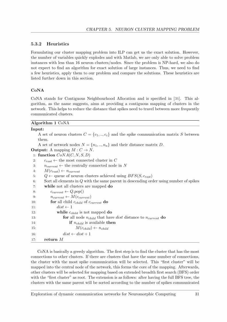
CoNA

CoNA stands for Contiguous Neighbourhood Allocation and is specified in [36]. This al-gorithm, as the name suggests, aims at providing a contiguous mapping of clusters in thenetwork. This helps to reduce the distance that spikes need to travel between more frequentlycommunicated clusters.

Algorithm 1 CoNA

Input:A set of neuron clusters C = {c1, .., cc} and the spike communication matrix S betweenthem.A set of network nodes N = {n1, .., nn} and their distance matrix D.

Output: A mapping M : C → N .1: function CoNA(C,N, S,D)2: croot ← the most connected cluster in C3: ncurrent ← the centrally connected node in N4: M(croot)← ncurrent5: Q← queue of neuron clusters achieved using BFS(S, croot)6: Sort all elements in Q with the same parent in descending order using number of spikes7: while not all clusters are mapped do8: ccurrent ← Q.pop()9: ncurrent ←M(ccurrent)

10: for all child cchild of ccurrent do11: dist← 112: while cchild is not mapped do13: for all node nchild that have dist distance to ncurrent do14: if nchild is available then15: M(cchild)← nchild

16: dist← dist+ 1

17: return M

CoNA is basically a greedy algorithm. The first step is to find the cluster that has the mostconnections to other clusters. If there are clusters that have the same number of connections,the cluster with the most spike communication will be selected. This “first cluster” will bemapped into the central node of the network, this forms the core of the mapping. Afterwards,other clusters will be selected for mapping based on extended breadth first search (BFS) orderwith the “first cluster” as root. The extension is as follows: after having the full BFS tree, theclusters with the same parent will be sorted according to the number of spikes communicated



to the parent cluster. This is to prioritise more frequent communication. For a cluster, thenode to be mapped on is chosen based on the smallest distance available to the node that itsparent is mapped on. This is carried out until all clusters are mapped.

Complexity analysis: For the worst case of n neuron clusters all connected together, asearch for the most connected cluster takes O(n2) time. A BFS perform on S is also of O(n2)complexity. Line 6 in the algorithm takes O(nlogn) time. Both the outer while and for loopin line 7 and 10 terminate after all n clusters are mapped. If we pre-sort the distance matrix forevery node, the while loop in line 12 takes O(n) time in the worst case to search for a node.The distance sorting itself takes O(n2logn) time. Thus, the whole CoNA algorithm takesO(n2) + O(n2) + O(nlogn) + O(n2) + O(n2logn) time, which is of O(n2logn) complexity.

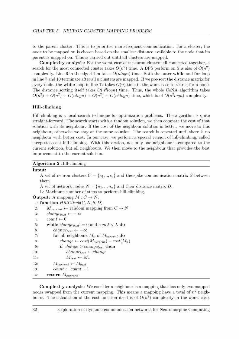
Hill-climbing

Hill-climbing is a local search technique for optimization problems. The algorithm is quitestraight-forward: The search starts with a random solution, we then compare the cost of thatsolution with its neighbour. If the cost of the neighbour solution is better, we move to thisneighbour, otherwise we stay at the same solution. The search is repeated until there is noneighbour with better cost. In our case, we perform a special version of hill-climbing, calledsteepest ascent hill-climbing. With this version, not only one neighbour is compared to thecurrent solution, but all neighbours. We then move to the neighbour that provides the bestimprovement to the current solution.

Algorithm 2 Hill-climbing

Input:A set of neuron clusters C = {c1, .., cc} and the spike communication matrix S betweenthem.A set of network nodes N = {n1, .., nn} and their distance matrix D.L: Maximum number of steps to perform hill-climbing

Output: A mapping M : C → N .1: function HillClimb(C,N, S,D)2: Mcurrent ← random mapping from C → N3: changebest ← −∞4: count← 05: while changebest! = 0 and count < L do6: changebest ← −∞7: for all neighbours Mn of Mcurrent do8: change← cost(Mcurrent)− cost(Mn)9: if change > changebest then

10: changebest ← change11: Mbest ←Mn

12: Mcurrent ←Mbest

13: count← count+ 1

14: return Mcurrent

Complexity analysis: We consider a neighbour is a mapping that has only two mappednodes swapped from the current mapping. This means a mapping have a total of n2 neigh-bours. The calculation of the cost function itself is of O(n2) complexity in the worst case.



If we put extra condition to prevent hill-climbing from performing an exhaustive search, thewhile loop in line 4 of the algorithm will repeat maximum L times. Thus hill-climb is ofO(Ln4) complexity.

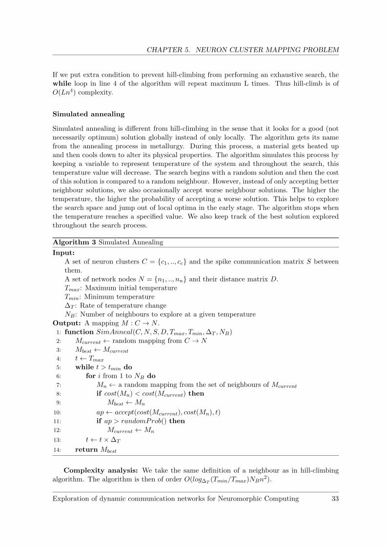
Simulated annealing

Simulated annealing is different from hill-climbing in the sense that it looks for a good (notnecessarily optimum) solution globally instead of only locally. The algorithm gets its namefrom the annealing process in metallurgy. During this process, a material gets heated upand then cools down to alter its physical properties. The algorithm simulates this process bykeeping a variable to represent temperature of the system and throughout the search, thistemperature value will decrease. The search begins with a random solution and then the costof this solution is compared to a random neighbour. However, instead of only accepting betterneighbour solutions, we also occasionally accept worse neighbour solutions. The higher thetemperature, the higher the probability of accepting a worse solution. This helps to explorethe search space and jump out of local optima in the early stage. The algorithm stops whenthe temperature reaches a specified value. We also keep track of the best solution exploredthroughout the search process.

Algorithm 3 Simulated Annealing

Input:A set of neuron clusters C = {c1, .., cc} and the spike communication matrix S betweenthem.A set of network nodes N = {n1, .., nn} and their distance matrix D.Tmax: Maximum initial temperatureTmin: Minimum temperature∆T : Rate of temperature changeNB: Number of neighbours to explore at a given temperature

Output: A mapping M : C → N .1: function SimAnneal(C,N, S,D, Tmax, Tmin,∆T , NB)2: Mcurrent ← random mapping from C → N3: Mbest ←Mcurrent

4: t← Tmax5: while t > tmin do6: for i from 1 to NB do7: Mn ← a random mapping from the set of neighbours of Mcurrent

8: if cost(Mn) < cost(Mcurrent) then9: Mbest ←Mn

10: ap← accept(cost(Mcurrent), cost(Mn), t)11: if ap > randomProb() then12: Mcurrent ←Mn

13: t← t×∆T

14: return Mbest

Complexity analysis: We take the same definition of a neighbour as in hill-climbingalgorithm. The algorithm is then of order O(log∆T

(Tmin/Tmax)NBn2).



5.4 Solution comparison

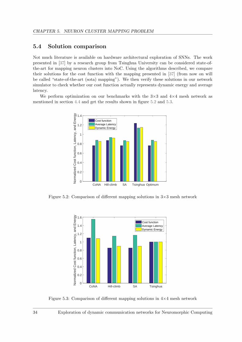
Not much literature is available on hardware architectural exploration of SNNs. The workpresented in [37] by a research group from Tsinghua University can be considered state-of-the-art for mapping neuron clusters into NoC. Using the algorithms described, we comparetheir solutions for the cost function with the mapping presented in [37] (from now on willbe called “state-of-the-art (sota) mapping”). We then verify these solutions in our networksimulator to check whether our cost function actually represents dynamic energy and averagelatency.

We perform optimization on our benchmarks with the 3×3 and 4×4 mesh network asmentioned in section 4.4 and get the results shown in figure 5.2 and 5.3.

CoNA Hill-climb SA Tsinghua Optimum0

0.2

0.4

0.6

0.8

1

1.2

1.4

Nor

mal

ized

Cos

t fun

ctio

n, L

aten

cy, a

nd E

nerg

y

Cost functionAverage LatencyDynamic Energy

Figure 5.2: Comparison of different mapping solutions in 3×3 mesh network

CoNA Hill-climb SA Tsinghua0

0.2

0.4

0.6

0.8

1

1.2

1.4

1.6

Nor

mal

ized

Cos

t fun

ctio

n, L

aten

cy, a

nd E

nerg

y





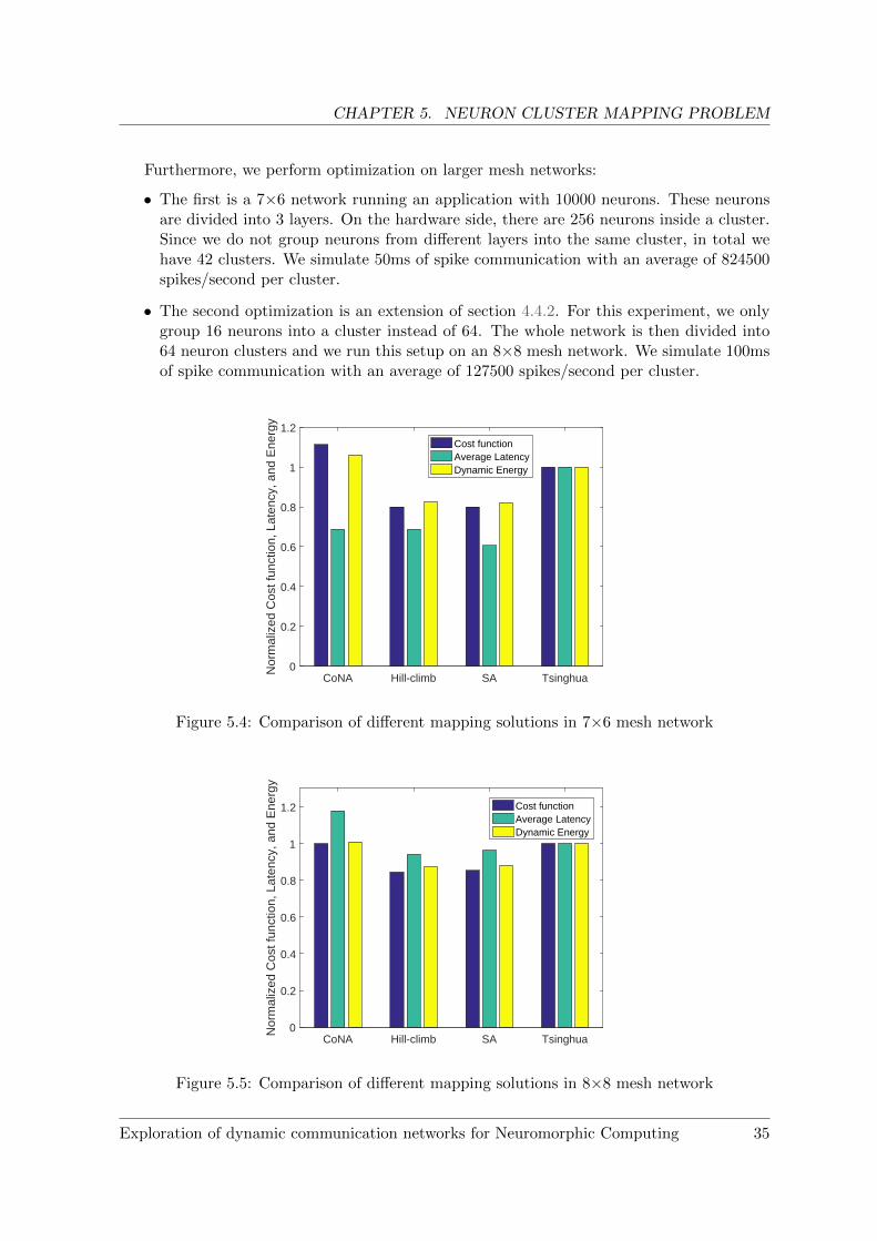
Furthermore, we perform optimization on larger mesh networks:

• The first is a 7×6 network running an application with 10000 neurons. These neuronsare divided into 3 layers. On the hardware side, there are 256 neurons inside a cluster.Since we do not group neurons from different layers into the same cluster, in total wehave 42 clusters. We simulate 50ms of spike communication with an average of 824500spikes/second per cluster.

• The second optimization is an extension of section 4.4.2. For this experiment, we onlygroup 16 neurons into a cluster instead of 64. The whole network is then divided into64 neuron clusters and we run this setup on an 8×8 mesh network. We simulate 100msof spike communication with an average of 127500 spikes/second per cluster.


0.2

0.4

0.6

0.8

1

1.2

Nor

mal

ized

Cos

t fun

ctio

n, L

aten

cy, a

nd E

nerg

y




0.2

0.4

0.6

0.8

1

1.2

Nor

mal

ized

Cos

t fun

ctio

n, L

aten

cy, a

nd E

nerg

y





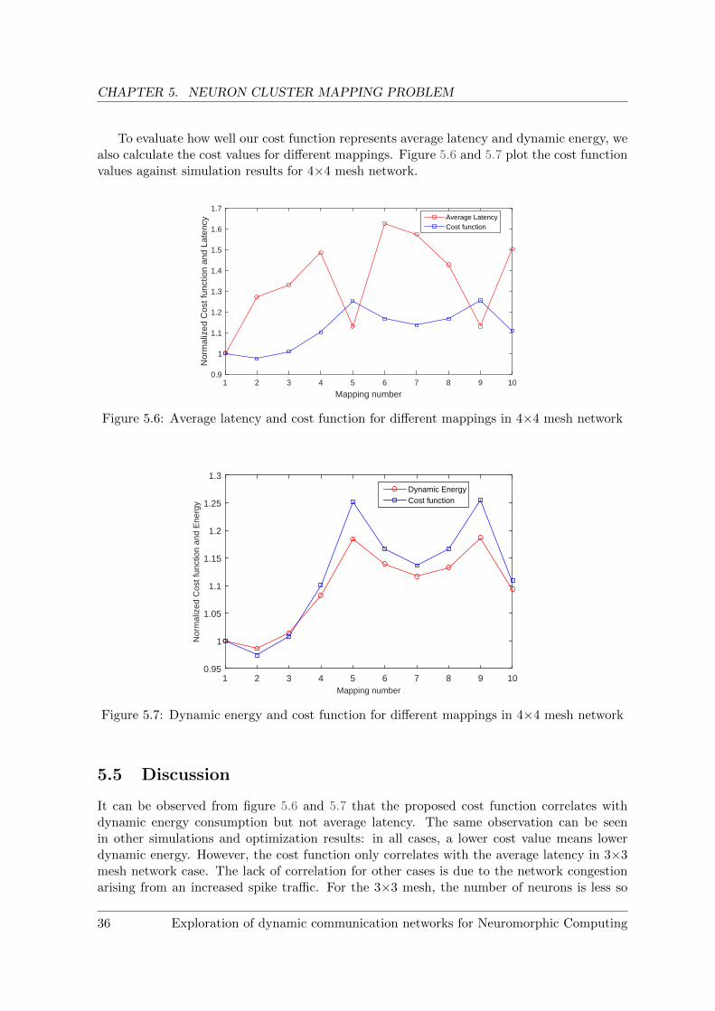
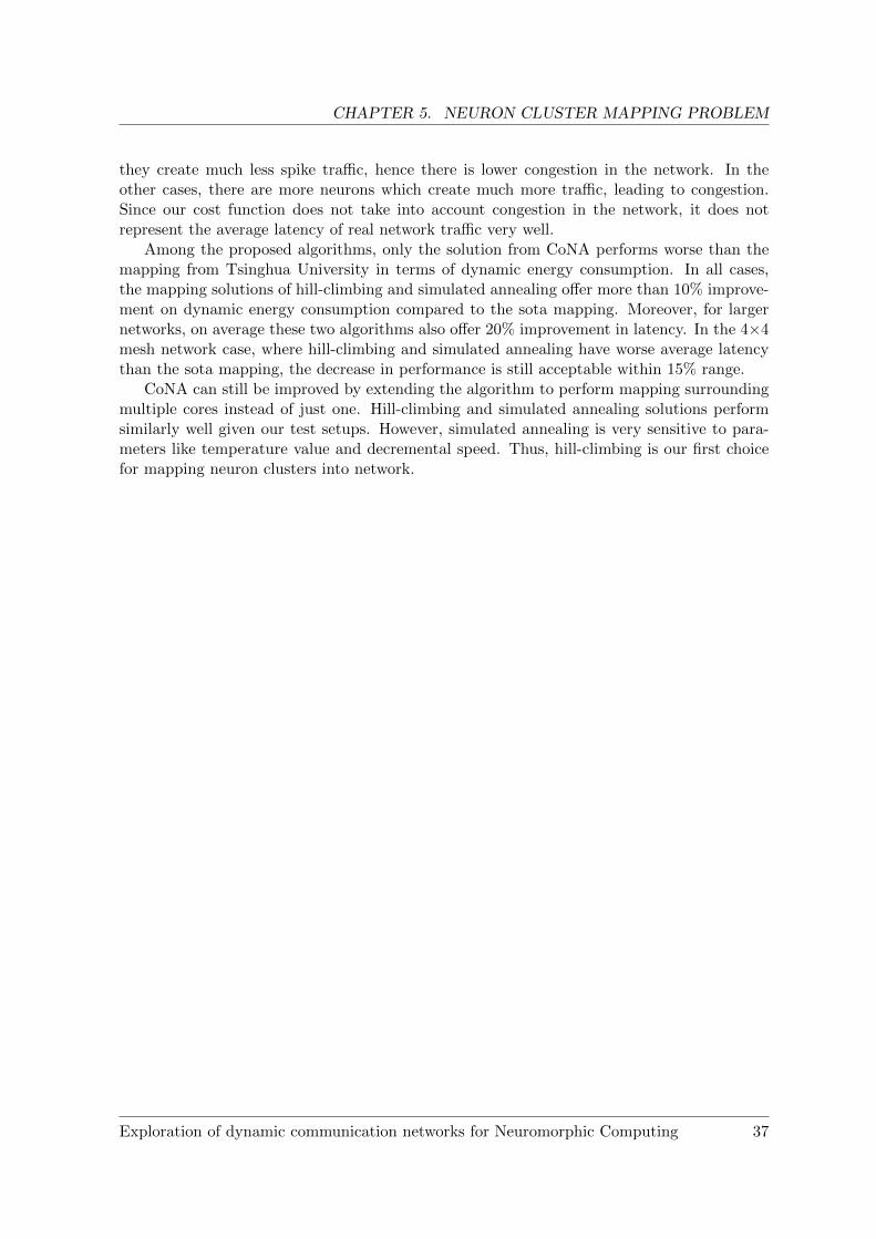
To evaluate how well our cost function represents average latency and dynamic energy, wealso calculate the cost values for different mappings. Figure 5.6 and 5.7 plot the cost functionvalues against simulation results for 4×4 mesh network.

Mapping number1 2 3 4 5 6 7 8 9 10

Nor

mal

ized

Cos

t fun

ctio

n an

d La

tenc

y

0.9

1

1.1

1.2

1.3

1.4

1.5

1.6

1.7Average LatencyCost function

Figure 5.6: Average latency and cost function for different mappings in 4×4 mesh network

Mapping number1 2 3 4 5 6 7 8 9 10

Nor

mal

ized

Cos

t fun

ctio

n an

d E

nerg

y

0.95

1

1.05

1.1

1.15

1.2

1.25

1.3

Dynamic EnergyCost function

Figure 5.7: Dynamic energy and cost function for different mappings in 4×4 mesh network

5.5 Discussion

It can be observed from figure 5.6 and 5.7 that the proposed cost function correlates withdynamic energy consumption but not average latency. The same observation can be seenin other simulations and optimization results: in all cases, a lower cost value means lowerdynamic energy. However, the cost function only correlates with the average latency in 3×3mesh network case. The lack of correlation for other cases is due to the network congestionarising from an increased spike traffic. For the 3×3 mesh, the number of neurons is less so



they create much less spike traffic, hence there is lower congestion in the network. In theother cases, there are more neurons which create much more traffic, leading to congestion.Since our cost function does not take into account congestion in the network, it does notrepresent the average latency of real network traffic very well.

Among the proposed algorithms, only the solution from CoNA performs worse than themapping from Tsinghua University in terms of dynamic energy consumption. In all cases,the mapping solutions of hill-climbing and simulated annealing offer more than 10% improve-ment on dynamic energy consumption compared to the sota mapping. Moreover, for largernetworks, on average these two algorithms also offer 20% improvement in latency. In the 4×4mesh network case, where hill-climbing and simulated annealing have worse average latencythan the sota mapping, the decrease in performance is still acceptable within 15% range.

CoNA can still be improved by extending the algorithm to perform mapping surroundingmultiple cores instead of just one. Hill-climbing and simulated annealing solutions performsimilarly well given our test setups. However, simulated annealing is very sensitive to para-meters like temperature value and decremental speed. Thus, hill-climbing is our first choicefor mapping neuron clusters into network.


Chapter 6

Conclusion and Future Work

6.1 Conclusion

In this project, a wide variety of topics are studied, ranging from Machine Learning al-gorithms, neuromorphic computing models, interconnect networks, software architecture toheuristic techniques for optimization. These are but a small part of the whole complex processfor building low-power hardware devices to run spiking neural network - Machine Learningapplications.

We have successfully built a hardware network simulator that can accept spike communic-ation input from an application-level simulator. This simulator can perform cycle-accuratesimulations and scale up to medium- sized networks (10000 neuron clusters). Using thissimulator, we carried out experiments to identify performance issues in mesh network.

With the information obtained from the intermediate simulation results, we formulatedan optimization problem for mapping neuron clusters. Then, we researched and proposedmultiple algorithms to solve this problem. Incorporating the solutions provided by thesealgorithms into the network simulator, we verified that our mapping solutions offer at least10% reduction in dynamic energy consumption compared to the state-of-the-art mapping.Furthermore, in most cases, our mapping solutions also provide 20% improvement in averagelatency.

Although mesh networks do not offer great flexibility, while there are improvements andoptimization that can be made, they are still good candidates for large scale, global-levelneuromorphic interconnect.

6.2 Future work

As this thesis is just the starting phase of a much bigger project, there is a lot of scope forextending this work. On the optimization side, the cost function to find an optimum mappingof neuron clusters can be improved to incorporate latency. This improvement can be carriedout for any fixed routing algorithm by pre-calculating the route for communication betweennetwork nodes. Similar to [38], the new cost function then need to integrate this informationto impose higher cost proportional to the number of overlapped communication links and theamount of spike traffic that occurs on those links.

The same optimization cost function can be used to explore segmented bus network fordynamic energy consumption. Here, the distance between two neuron clusters is represented


CHAPTER 6. CONCLUSION AND FUTURE WORK

by the number of switches on the shortest path between them. However, the extension of thecost function suggested above might not be suitable for this architecture, since the routingwill be dynamic and carried out in software.

On the simulator implementation side, it would be interesting to see how a multicast routerperforms in a mesh network. In most of the cases, the number of fan-outs for a neuron willbe larger than the number of neurons in a cluster. This means a spike message would need tobe sent to multiple clusters. A multicast router would help to reduce traffic load inside suchnetworks.

Additionally, we also need to speed up the simulator for large neural networks by imple-menting transaction level modelling (TLM) that is available in SystemC.

After the proposed network topologies are implemented and simulation speed is improved,we can also try to incorporate a model of neuron clusters into the simulator. This will helpto create a full simulation platform to study the effect of hardware implementation of neuralnetwork at the application level.


Bibliography

[1] F. Dell’Anna, “Interface between RTL and application neuromorphic simulator,” 2016.2

[2] W. Maass, “Networks of spiking neurons: The third generation of neural networkmodels,” Neural Networks, vol. 10, no. 9, pp. 1659 – 1671, 1997. [Online]. Available:http://www.sciencedirect.com/science/article/pii/S0893608097000117 4

[3] W. S. McCulloch and W. Pitts, “A logical calculus of the ideas immanent in nervousactivity,” Bulletin of Mathematical Biophysics, 1943. 4

[4] Y. Lecun, L. Bottou, Y. Bengio, and P. Haffner, “Gradient-based learning applied todocument recognition,” Proceedings of the IEEE, 1998. 7

[5] S. Hochreiter and J. Schmidhuber, “Long short-term memory,” Neural Comput., vol. 9,no. 8, pp. 1735–1780, Nov. 1997. [Online]. Available: http://dx.doi.org/10.1162/neco.1997.9.8.1735 7

[6] H. Jaeger. (2007) Echo state network. [Online]. Available: http://www.scholarpedia.org/article/Echo state network 7

[7] J. Hopfield, “Neural networks and physical systems with emergent collective computa-tional abilities,” Proceedings of the National Academy of Sciences of the United States ofAmerica, 1982. 7

[8] G. E. Hinton, S. Osindero, and Y.-W. Teh, “A fast learning algorithm for deep beliefnets,” Neural Comput., vol. 18, no. 7, pp. 1527–1554, Jul. 2006. [Online]. Available:http://dx.doi.org/10.1162/neco.2006.18.7.1527 8

[9] H. Larochelle, D. Erhan, A. Courville, J. Bergstra, and Y. Bengio, “An empiricalevaluation of deep architectures on problems with many factors of variation,”in Proceedings of the 24th International Conference on Machine Learning, ser.ICML ’07. New York, NY, USA: ACM, 2007, pp. 473–480. [Online]. Available:http://doi.acm.org/10.1145/1273496.1273556 8

[10] H. Lee, R. Grosse, R. Ranganath, and A. Y. Ng, “Convolutional deep beliefnetworks for scalable unsupervised learning of hierarchical representations,” inProceedings of the 26th Annual International Conference on Machine Learning, ser.ICML ’09. New York, NY, USA: ACM, 2009, pp. 609–616. [Online]. Available:http://doi.acm.org/10.1145/1553374.1553453 8

[11] Y. LeCun, Y. Bengio, and G. Hinton, “Deep learning,” Nature Review, 2015. 9


http://www.sciencedirect.com/science/article/pii/S0893608097000117

http://dx.doi.org/10.1162/neco.1997.9.8.1735


http://www.scholarpedia.org/article/Echo_state_network

http://www.scholarpedia.org/article/Echo_state_network


http://doi.acm.org/10.1145/1273496.1273556

http://doi.acm.org/10.1145/1553374.1553453

BIBLIOGRAPHY

[12] G.-Q. Bi and M.-M. Poo, “Synaptic modifications in cultured hippocampal neurons:Dependence on spike timing, synaptic strength, and postsynaptic cell type,” The Journalof Neuroscience, 1998. 10

[13] C. Mead, Analog VLSI and Neural Systems. Boston, MA, USA: Addison-Wesley Long-man Publishing Co., Inc., 1989. 10

[14] G. Indiveri, B. Linares-Barranco, T. J. Hamilton, A. van Schaik, R. Etienne-Cummings,T. Delbruck, S.-C. Liu, P. Dudek, P. Hfliger, S. Renaud, J. Schemmel, G. Cauwenberghs,J. Arthur, K. Hynna, F. Folowosele, S. SAGHI, T. Serrano-Gotarredona, J. Wijekoon,Y. Wang, and K. Boahen, “Neuromorphic silicon neuron circuits,” Frontiers inNeuroscience, vol. 5, no. 73, 2011. [Online]. Available: http://www.frontiersin.org/neuromorphic engineering/10.3389/fnins.2011.00073/abstract 10, 11

[15] N. Qiao, H. Mostafa, F. Corradi, M. Osswald, F. Stefanini, D. Sumislawska,and G. Indiveri, “A re-configurable on-line learning spiking neuromorphic processorcomprising 256 neurons and 128k synapses,” Frontiers in Neuroscience, vol. 9, no.141, 2015. [Online]. Available: http://www.frontiersin.org/neuromorphic engineering/10.3389/fnins.2015.00141/abstract 11

[16] P. O’Connor, D. Neil, S.-C. Liu, T. Delbruck, and M. Pfeiffer, “Real-time classification and sensor fusion with a spiking deep belief network,”Frontiers in Neuroscience, vol. 7, no. 178, 2013. [Online]. Available: http://www.frontiersin.org/neuromorphic engineering/10.3389/fnins.2013.00178/abstract 12

[17] P. U. Diehl, D. Neil, J. Binas, M. Cook, S.-C. Liu, and M. Pfeiffer, “Fast-classifying,high-accuracy spiking deep networks through weight and threshold balancing.” inIJCNN. IEEE, 2015, pp. 1–8. [Online]. Available: http://dblp.uni-trier.de/db/conf/ijcnn/ijcnn2015.html 12

[18] M. Mahowald, An Analog VLSI System for Stereoscopic Vision. Norwell, MA, USA:Kluwer Academic Publishers, 1994. 13

[19] K. A. Boahen, “Communication neuronal ensembles between neuromorphic chips.” 13

[20] D. S. Bassett and E. Bullmore, “Small-world brain networks,” The Neuroscientist,vol. 12, no. 6, pp. 512–523, 2006. [Online]. Available: http://nro.sagepub.com/content/12/6/512.abstract 13

[21] G. Indiveri, F. Corradi, and N. Qiao, “Neuromorphic architectures for spiking deep neuralnetworks,” in 2015 IEEE International Electron Devices Meeting (IEDM), Dec 2015, pp.4.2.1–4.2.4. 13

[22] S. Moradi, N. Imam, R. Manohar, and G. Indiveri, “A memory-efficient routing methodfor large-scale spiking neural networks,” in Circuit Theory and Design (ECCTD), 2013European Conference on, Sept 2013, pp. 1–4. 14, 17

[23] P. Merolla, J. Arthur, R. Alvarez-Icaza, A. Cassidy, J. Sawada, F. Akopyan, B. Jackson,N. Imam, C. Guo, Y. Nakamura, B. Brezzo, I. Vo, S. Esser, R. Appuswamy, B. Taba,A. Amir, M. Flickner, W. Risk, R. Manohar, and D. Modha, “A million spiking-neuronintegrated circuit with a scalable communication network and interface,” Science, pp.668–673, August 2014. 14


http://www.frontiersin.org/neuromorphic_engineering/10.3389/fnins.2011.00073/abstract






http://dblp.uni-trier.de/db/conf/ijcnn/ijcnn2015.html

http://dblp.uni-trier.de/db/conf/ijcnn/ijcnn2015.html

http://nro.sagepub.com/content/12/6/512.abstract

http://nro.sagepub.com/content/12/6/512.abstract

BIBLIOGRAPHY

[24] K. Heyrman, A. Papanikolaou, F. Catthoor, P. Veelaert, K. Debosschere, andW. Philips, Energy Consumption for Transport of Control Information on a SegmentedSoftware-Controlled Communication Architecture. Berlin, Heidelberg: Springer BerlinHeidelberg, 2006, pp. 52–58. [Online]. Available: http://dx.doi.org/10.1007/11802839 815

[25] L. Cai and D. Gajski, “Transaction level modeling: an overview,” in CODES+ISSS ’03:Proceedings of the 1st IEEE/ACM/IFIP International Conference on Hardware/softwareCodesign and System Synthesis. New York, NY, USA: ACM Press, 2003, pp. 19–24.[Online]. Available: http://doi.acm.org/10.1145/944645.944651 18

[26] N. Jiang, D. U. Becker, G. Michelogiannakis, J. D. Balfour, B. Towles, D. E. Shaw,J. Kim, and W. J. Dally, “A detailed and flexible cycle-accurate network-on-chipsimulator,” in 2012 IEEE International Symposium on Performance Analysis of Systems& Software, Austin, TX, USA, 21-23 April, 2013, 2013, pp. 86–96. [Online]. Available:http://dx.doi.org/10.1109/ISPASS.2013.6557149 19

[27] J. M. Joseph and T. Pionteck, “A cycle-accurate network-on-chip simulator with sup-port for abstract task graph modeling,” in System-on-Chip (SoC), 2014 InternationalSymposium on, Oct 2014, pp. 1–6. 19

[28] Atlas main page. [Online]. Available: https://corfu.pucrs.br/redmine/projects/atlas 19

[29] V. Catania, A. Mineo, S. Monteleone, M. Palesi, and D. Patti, “Noxim: An open,extensible and cycle-accurate network on chip simulator,” in 26th IEEE InternationalConference on Application-specific Systems, Architectures and Processors, ASAP 2015,Toronto, ON, Canada, July 27-29, 2015, 2015, pp. 162–163. [Online]. Available:http://dx.doi.org/10.1109/ASAP.2015.7245728 20

[30] Nirgam main page. [Online]. Available: http://nirgam.ecs.soton.ac.uk/home.php 20

[31] M. Lis, P. Ren, M. H. Cho, K. S. Shim, C. W. Fletcher, O. Khan, and S. Devadas,“Scalable, accurate multicore simulation in the 1000-core era,” in Performance Analysisof Systems and Software (ISPASS), 2011 IEEE International Symposium on, April 2011,pp. 175–185. 20

[32] R. E. Burkard, E. ela, P. M. Pardalos, and L. S. Pitsoulis, “The quadratic assignmentproblem,” 1998. 29

[33] S. Sahni and T. Gonzalez, “P-complete approximation problems,” J. ACM, vol. 23,no. 3, pp. 555–565, Jul. 1976. [Online]. Available: http://doi.acm.org.dianus.libr.tue.nl/10.1145/321958.321975 29

[34] G. Laporte, “The traveling salesman problem: An overview of exact and approximatealgorithms,” European Journal of Operational Research, vol. 59, no. 2, pp. 231–247, June1992. [Online]. Available: https://ideas.repec.org/a/eee/ejores/v59y1992i2p231-247.html 29

[35] P. Rubin. Binary variables and quadratic terms. [Online]. Available: http://orinanobworld.blogspot.nl/2010/10/binary-variables-and-quadratic-terms.html 30


http://dx.doi.org/10.1007/11802839_8

http://doi.acm.org/10.1145/944645.944651

http://dx.doi.org/10.1109/ISPASS.2013.6557149

https://corfu.pucrs.br/redmine/projects/atlas

http://dx.doi.org/10.1109/ASAP.2015.7245728

http://nirgam.ecs.soton.ac.uk/home.php

http://doi.acm.org.dianus.libr.tue.nl/10.1145/321958.321975

http://doi.acm.org.dianus.libr.tue.nl/10.1145/321958.321975

https://ideas.repec.org/a/eee/ejores/v59y1992i2p231-247.html

https://ideas.repec.org/a/eee/ejores/v59y1992i2p231-247.html

http://orinanobworld.blogspot.nl/2010/10/binary-variables-and-quadratic-terms.html

http://orinanobworld.blogspot.nl/2010/10/binary-variables-and-quadratic-terms.html

BIBLIOGRAPHY

[36] M. Fattah, M. Ramirez, M. Daneshtalab, P. Liljeberg, and J. Plosila, “Cona: Dynamicapplication mapping for congestion reduction in many-core systems,” in Computer Design(ICCD), 2012 IEEE 30th International Conference on, Sept 2012, pp. 364–370. 31

[37] Y. Ji, Y.-H. Zhang, and W.-M. Zheng, “Modelling spiking neural networkfrom the architecture evaluation perspective,” Journal of Computer Scienceand Technology, vol. 31, no. 1, pp. 50–59, 2016. [Online]. Available: http://dx.doi.org/10.1007/s11390-016-1611-0 34

[38] C.-L. Chou and R. Marculescu, “Contention-aware application mapping for network-on-chip communication architectures,” in Computer Design, 2008. ICCD 2008. IEEEInternational Conference on, Oct 2008, pp. 164–169. 38


http://dx.doi.org/10.1007/s11390-016-1611-0

http://dx.doi.org/10.1007/s11390-016-1611-0

Documents

Eindhoven University of Technology MASTER Exploration of ... · Exploration of dynamic communication networks for Neuromorphic Computing Master Thesis Khanh Huynh Department of Electrical