Eindhoven University of Technology

MASTER

Multipoint Video Distribution System (MVDS) in the 28 GHz and the 42 GHz frequencybands

Vugts, J.A.G.

Award date:1995

DisclaimerThis document contains a student thesis (bachelor's or master's), as authored by a student at Eindhoven University of Technology. Studenttheses are made available in the TU/e repository upon obtaining the required degree. The grade received is not published on the documentas presented in the repository. The required complexity or quality of research of student theses may vary by program, and the requiredminimum study period may vary in duration.

General rightsCopyright and moral rights for the publications made accessible in the public portal are retained by the authors and/or other copyright ownersand it is a condition of accessing publications that users recognise and abide by the legal requirements associated with these rights.

• Users may download and print one copy of any publication from the public portal for the purpose of private study or research. • You may not further distribute the material or use it for any profit-making activity or commercial gain

Take down policyIf you believe that this document breaches copyright please contact us providing details, and we will remove access to the work immediatelyand investigate your claim.

Download date: 26. Aug. 2018

Concerns:Period of work :

Eindhoven University of TechnologyFaculty of Electrical Engineering

Telecommunications division

Multipoint Video Distribution System(MVDS) in the 28 GHz and the 42 GHz

frequency bands

by

John J.A.G. Vugts.

Graduation projectNovember 1994 - June 1995

Supervisors: ir. P.G.M. de Bot (Philips)prof. dr. ir. G. Brussaard (TUE)ir. J. Dijk (TUE)

Eindhoven, June 1995

The Faculty of Electrical Engineering of the EindhovenUniversity of Technology is not responsible for the contents of

practical work reports and graduate reports.

Author

Title

Abstract

John J.A.G. Vugts

Multipoint Video Distribution System (MVDS) in the 28 GHz and the42 GHz frequency bands

Multipoint Video Distribution System (MVDS) is a terrestrial point-to-multipointradio system for distributing TV signals to the homes of end users as an alternativeto the conventional cable networks. Such a system is to be operated at high RFfrequencies (40.5-42.5 GHz) because of the relatively large bandwidth required whichis not available at lower frequencies. The objective of the work is to examine thepossibilities of MVDS in a Single-Frequency Network (SFN) and to see if a Line OfSight (LOS) is always required. This work results in a system proposal.

The propagation aspects such as refraction, diffraction, fading, attenuation etc. ofthe 42 GHz electromagnetic waves have been examined. Furthermore the possib­ilities and effects of refiection on building materials is examined. There has beenanalytically shown that the increase in coverage due to diffraction is negligible.

Measurements have been performed which showed that the link-budget calculationswere accurate. They also gave an indication of the loss due to foliage (20-30 dB),refiection coefficients (10 dB) and the negligible possibilities of using diffraction andrefiection. They also showed that multipath reception can be prevented largely byusing narrow beam reception antennas.

A program has been written which predicts the percentage of coverage within aspecific area and a model of Eindhoven has been created. With these tools it isshown that the increase in the percentage of coverage due to refiections is negligiblefor a typical Dutch city. This is due to the lack of appropriate refiection surfacesin such an environment and the small refiection coefficients of rough surfaces. Thepercentage of the cell surface which is covered depends very much on the heights ofthe buildings and the antennas.

Research on networks has been done to assess the feasibility of SFNs. Both omni­directional antennas and directional antennas have been used to find a good solutionof the SFN problem. Using directional antennas resulted in an SFN using twopolarizations (CjI of 11 dB). The performance degradation due to the interferenceis calculated and simulated. The CIR found in the proposed network can be dealtwith using the built in error correction capabilities. Three different schemes aregiven to feed the celluiar SFN network.

It is found that an example system with typical parameters has a ceU diameter of4.69 km and can support in the band 40.5 42.5 GHz up to 48 channels (41.6 MHzspacing), corresponding to 336 different programs.

1

Contents

1 Introduction 1

2 Multipoint Video Distribution 8ystem (MVD8) 2

2.1 Introduction .. 2

2.2 Cellular system 2

2.3 System description of the current analog system 3

2.4 Description of the digital system 4

2.4.1 Transmitter description . 4

2.4.2 Receiver description 12

2.5 Discussion . . . . ...... 14

3 Propagation aspects 15

3.1 Free space . 15

3.2 Refractivity 16

3.3 Diffraction . 18

3.4 Diffraction around obstacles 20

3.5 Reflections . . . . . . . . . . 27

3.5.1 Fresnel reflection coefficients 30

3.5.2 Reflection model of thin layers . 33

3.5.3 Reflection at rough surfaces 34

3.6 Power fading (flat fading) ..... 39

3.7 Fading due to multipath propagation (frequency selective fading) 41

3.8 Rain attenuation 44

3.9 ITU-R rain model. 45

3.10 Cross-polar discrimination 48

iii

3.11 Sky noise temperature

3.12 Discussion ...

4 Network topology

4.1 Cellular systems using omni directional antennas .

4.2 Cellular systems using directional antennas ....

4.2.1 One direction Hne-up of the transmitter antennas

4.2.2 Rotated Hne-up of the transmitter antennas

4.2.3 Rotated Hne-up using both polarizations

4.3 Feeding of single frequency networks

4.3.1 Optical feeding of the network .

4.3.2 Feeding the network by satellite

4.3.3 Mutual feeding of the network .

4.4 Discussion .

5 Link budget calculations

5.1 Tolerabie noise and interference .

5.1.1 Influence of the Nyquist filter on the noise power

5.1.2 Influence of noise on the QPSK performance

5.1.3 Influence of interference on the QPSK performance

5.1.4 Worst case interference model

5.2 Link budget with noise .

5.3 Link budget with noise and interference .

5.4 Link budget for the feeding network .

5.5 Discussion . . . . . . . . . . . . . . .

6 Expected coverage in a city

6.1 Line of sight coverage ...

6.2 Coverage using reflections

6.3 Discussion . . . . . . . . .

54

55

56

57

59

61

62

63

65

65

66

66

67

68

68

68

71

73

74

78

85

86

86

90

92

93

94

7 Measurements 98

7.1 Link budget verification 99

IV

7.2 Reflection .100

7.3 Diffraction . · 103

704 Depolarization . · 103

7.5 Discussion . . . · 103

8 Conclusions and recommendations 104

8.1 Conclusions .... · 104

8.2 Recommendations . · 106

9 Acknowledgements 108

References 109

A Analog system description 113

A.I Indoor transmit unit · 113

A.2 Outdoor transmit unit · 113

A.3 Transmitter antenna · 114

AA Receiver antenna .. · 116

A.5 Outdoor receive unit · 118

A.6 Indoor receive unit · 118

B Power decay rate 119

C Snellius law for a round earth 121

D Diffraction 125

v

List of Symbols and Acronyms

a earth radius [km]ae effective earth radius [km]B bandwidth [Hz]Be transponder bandwidth [MHz]Bn Nyquist bandwidth [MHz]BER bit error rate [S-1 ]c carrier power [W]c velocity of an electromagnetic wave in a vacuum tm/sjC carrier power [dBW]CATV cable television system []CNR carrier to noise ratio [dB]CIR carrier to interference ratio [dB]cl fresnel zone clearance [m]d path length (distance) [m]d Hamming distance []D antenna diameter [m]e water vapour pressure [mbar]E received field strength [V/m]E average electric field [V/m]Et transversal electric field [V/m]eirp effective isotropic radiated power [W]EIRP effective isotropic radiated power [dBW]Eo direct wave field strength [V/m]Es symbol energy [Ws]

f frequency [Hz]FEC forward error correction []F noise figure [dB]G gain [dB]GU) power spectral density function [dB]Gn(j) power spectral density function lW/Hz]9r receiver antenna gain []Gr receiver antenna gain [dB]

9t transmitter antenna gain []Gt transmitter antenna gain [dB]

vii

H(J)hr

Hr(J)ht

Ht

Ht(J)IkkklaLalbfLbf

leLdf

LfL feed

Lm

lmLFSRLOSLMDSlpLpMMDSMPEGMVDSnnnc(t)ns(t)NN

PPbPe

PtPwPP(W)QEFQPSKr

channel transfer functionreceiver antenna heightreceive filter (amplitude response)transmitter antenna heighttransversal magnetic fieldtransmit filter (amplitude response)interference powerk-factorBoltzmann's constantpropagation constantrain attenuationrain attenuationfree space lossfree space lossantenna feed lossdiffraction lossfade marginfeeding loss of the antennasmedium IOS8

medium losslinear feedback shift registerline of sight10cal multipoint distribution systcmpointing 10sspointing 10ssmultipoint microwave distribution systemmotion picture experts groupmultipoint video distribution systemnoise powerrefractivity indexnarrow band noise power spectrum (eosine)narrow band noise power spectrum (sine)noise powerrefractivityoutage time percentage over a whole yearprobability of a bit errorprobability of an errortransmitted poweroutage worst month time percentageatmospheric pressuretime fraction of W power receivedquasi error free operationquadrature phase shift keyingpath length reduction factor

Vlll

[][m][][m][Alm][][dBW][][11K][I/m][][dB][][dB][][dB][dB][dB][dB][][]o[]o[dB][][][][W][][][][dBW]o[][]D[W]o[mbar][][][]o

r radius of a eell [m]r(t) noise signal in time domain [V]R rain rate [mm/hr]R eonvolutional eoding rate 0R refleetivity 0Rn nth Fresnel zone radius [m]RP radiated power [dBM]Ru Reed Solomon eoding rate []Ra.Ol rain rate exeeeded 0.01 % of the year [mm/hr]s signal power [W]S signal power [dBW]Sav power flux density [W/m2

]

SFN single frequeney network []SNR signal to noise ratio [dB]Sy(J) voltage2 spectral density function [V2/Hz]T temperature [K]T transmission coefficient []Ta ambient temperature [K]Tant antenna noise temperature [K]Tr receiver noise temperature [K]Train rain temperature [K]Tsys system noise temperatllre [K]Tsky sky noise temperature [K]V velocity [mis]Vmedium velocity of an electromagnetic wave in a medium tm/sjY(J) signal in frequency domain [V]XPD cross-polar discrimination [dB]y(t) signal in time domain [V]

Q: roll-off factor []f3 effective aperture [m2

]

fr rain attenuation (CCIR model) [dB/km]f r relative electric permittivity []'T) power spectrum density white noise lW/Hz]À wave length [m]Jlr relative magnetie permeability []P reflection coefficient [kg/m3

]

pil parallel reflection coefficient []p.l orthogonal refleetion coefficient []Ps specular reflection eoefficient 0a electrical conductivity [nm]r time difference [sj1> power flux [W/m 2

]

'Ij; phase differenee due to path Iength difference []

ix

Chapter 1

Introduction

This report describes the graduation work for the department of Electrical Engin­eering of the Eindhoven University of Technology. The research is in the field ofcommunications engineering. The research is carried out at Philips Research inEindhoven during the period November 1994 - June 1995.

The work is related to a Multipoint Video Distribution System (MVDS). MultipointVideo Distribution System (MVDS) is a terrestrial point-to-multipoint radio systemfor distributing TV signals to the homes of end users as an alternative to the con­ventional cable networks. Therefore it is also referred to as "Wireless cable". Sucha system is to be operated at high RF frequencies because of the large amount ofspectrum required which is not available at lower frequencies. For research purposes,an experimental 28 GHz single channellink has been installed at Philips.

With this link the propagation aspects which are of concern for a MVDS are in­vestigated. The objective of the work is to examine the possibilities of MVDS in aSingle-Frequency Network (SFN), to see if a Line Of Sight (LOS) is always requiredfor good reception, the planning of the cellular network and to see if it is possibleto have a Single frequency network (SFN). Therefore it is important to investigatethe coverage area, signal attenuation, shielding of buildings within the covered area,reuse distances and acceptable interference levels. For research on interference fromdifferent ceIls, a second transmitter is available. Theoretical models will predict theallowable carrier to interference ratio C/ I. Using the trial results of the analog linkit can be verified if this criteria can be met.

In Chapter 2 a general discussion of an MVDS system is given. In Chapter 3 thepropagation aspects will be discussed. In the following Chapter the different topo­logies of the networks are diseussed. The influenee of the interference is discussedin Chapter 5j from there the link-budgets can be ealculated. If the cell sizes areknown, one is interested in the percentage of coverage in a eeIl, this is discussed inChapter 6. To confirm the theories measurements are performed which are discussedin Chapter 7. In the final Chapter some conclusions and suggestions for further workare given.

1

Chapter 2

Multipoint Video DistributionSystem (MVDS)

2.1 Introduction

Multipoint Video Distribution Systems (MVDS)l are systems to provide a meansfor wireless local distribution of television services. They may be employed as analternative or a supplement to the cable TV distribution systems (CATV). Thesystem described here is a microwave multipoint video distribution system operatingin the 27.5-29.5 GHz range and a future system operating in the 40.5 GHz-42.5 GHzrange.

The first trial used a single 28 GHz link which enabled us to acquire practicalpropagation information. In the next step a second transmitter is involved to acquireinformation on single frequency network behaviour and to investigate the toleranceof the link to interference.

The future MVDS system will be a digital system based on the Digital Video Broad­casting (DVB) satellite standard. This is because of the availability of the systemcomponents. This results in a relatively inexpensive solution for digital MVDS.

2.2 Cellular system

To cover a large area with limited power, it is necessary to use multiple cells. Thetotal area to be covered is then divided in a number of subsections. Every subsectionhas its own transmitter. Since simple reuse of frequency in the adjacent cell wouldresult in strong interference near the edge of the cell, it is necessary to use a moresophisticated system. The most simple of course is to use different frequenciesin different cells, although this is very inefficient. The reuse distance depends on

1In the USA, the systems are known as Multipoint Microwave Distribution Systems (MMDS)

2

e.g. antenna gain patterns and on natural attenuation. The reuse distance can beshortened by using frequency offset, orthogonal-polarization and very narrow-beamreception antennas. The frequency offset is of no use in our system because of theoverlapping of the channels as discussed in Section 5.1.

The ultimate situation will obvious be a single frequency network where in all theadjacent cells the same frequency can be reused with acceptable interference. Thepossibilities for a single frequency network will be described in Section 4.

2.3 System description of the current analog sys­tem

In Appendix A there will be a short overview of the available system presented. InFigure 2.1 agiobal overview of the totallink is given.

PAL

Signal souree

Pre-emphasis

Power supply

Indoor transmitunit

FM modulator

unn Oscillato

Outdoor transmitunit

Transmitter antenna

Mixer

amplifier

SatelliteTuner

DemodulationDe-emphasis

PAL

Display souree

Outdoor receiveunit

Indoor receiveunit

Figure 2.1: Global overview of the link

All the blocks except the PAL source and the PAL TV in Figure 2.1 will be individu­ally described in Appendix A. The system description is a copy of the descriptionin [39]. Although the system is an analog FM modulated system propagation effectsetc. with this link can be studied. This information can then be extrapolated to adigital 42 GHz system which will be used in the future.

3

2.4 Description of the digital system

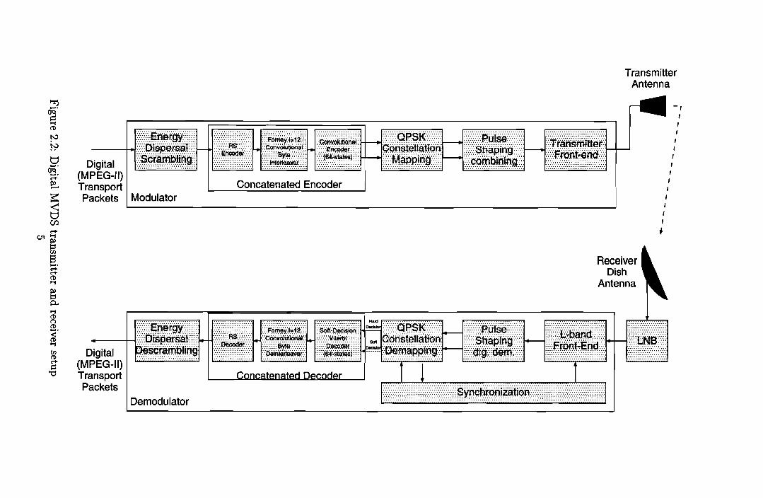
The future digital system used for MVDS will use the channel coding and modulationof the digital satellite system defined by Digital Video Broadcasting (DVB)[13, 14].This ensures that there will be very little additional costs involved in developinga digital MVDS receiver system. In principle a standard digital satellite receiverwith a special designed down converter can be used. The low noise block convertershifts the 42 GHz frequency range in one or two steps down to L-band, the desiredfrequency range for the standard satellite receiver. From that point onwards thestandard digital satellite demodulation equipment can be used. In Figure 2.2 thetransmitter and receiver setup is shown.

The only differences between the digital satellite scheme and the MVDS schemeare the transmitter front-end and the receiver LNB which convert the signal to andfrom 42 GHz respectively. The individual blocks in the link will be briefiy describedbelow [38].

The satellite system (digital MVDS system) uses QPSK-modulation. The forwarderror correction (FEe) of the satellite system consists of concatenated coding withReed-Solomon outer coding and convolutional inner coding.

2.4.1 Transmitter description

The bit stream to be transmitted is build up of MPEG-2 packets that contain 187data bytes and one synchronization byte. The MPEG-2 data structure is beyondthe scope of this report.

Energy dispersal scrambling

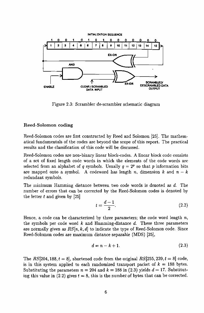
In order to comply with radio regulations and to ensure adequate binary transitions,the data will be scrambled. The scrambling method is based on a pseudo-randombit sequence. This sequence has a fiat power spectrum, so the energy will be equallydispersed over the whole spectrum [5]. The pseudo-random sequence is generated bya shift register with linear feedback (LFSR). The polynomial of the LFSR is givenby

1 + X 14 + X 15•

In Figure 2.3 the implementation is shown [13].

4

(2.1)

TransmitterAntenna

~-,'III,

I,IIIII,

I

#

ReceiverDish

Antenna

jî~ •••~;ä~.~: :i~i~~~;~i!~g~c~.;~~Concatenated Encoder

!I~.!.~!I!; ~_a!lf~:=I~II,!-i!It'J!+-llllL-.Cooc.ateIJ..a1ed....Ol~ aood.eL~ l! 1

}:·:··::·t··{:···{:::::::··///{:::::$.{fu#.*#.b.j~~#?:Bt}\::·:/:::::Itt:::.::IIIIII

Modulator

Demodulator

Digital(MPEG-II)TransportPackets

Digital(MPEG-II)TransportPackets

INlTIAllZATrON SEQUENCE

1001010100 00000

~ 1 1 2 I3 I 4 16 1e T 7-' a l~ 11 -1 12 /13 114 115 ~

ENABLE

AND

A"î----)D~-SCRAMBLE-----+) DIex-OR OESCRAMBlED o·o.!"

ClEAR I SCRAMBLEO "".......... ...DATA ".PUT VU.r-UI

Figure 2.3: Scrambler de-scrambler schematic diagram

Reed-Solomon coding

Reed-Solomon codes are first constructed by Reed and Solomon [25]. The mathem­atical fundamentals of the codes are beyond the scope of this report. The practicalresults and the c1assification of this code will be discussed.

Reed-Solomon codes are non-binary linear block-codes. A lincar block code consistsof a set of fixed length code words in which the elements of the code words areselected from an alphabet of q symbols. Usually q = 2P so that pinformation bitsare mapped onto a symbol. A codeword has length n, dimension k and n - kredundant symbols.

The minimum Hamming distance between two code words is denoted as d. Thenumber of errors that can be corrected by the Reed-Solomon codes is denoted bythe letter tand given by [25]

d-1t= -2-' (2.2)

Hence, a code can be characterized by three parameters; the code word length n,the symbols per code word k and Hamming-distance d. These three parametersare normally given as RB[n, k, d] to indicate the type of Reed-Solomon code. SinceReed-Solomon codes are maximum distance separable (MDS) [25],

d=n-k+l. (2.3)

The RB[204, 188, t = 8], shortened code from the original RB[255, 239, t = 8] code,is in this system applied to each randomized transport packet of k = 188 bytes.Substituting the parameters n = 204 and k = 188 in (2.3) yields d = 17. Substitut­ing this value in (2.2) gives t = 8, this is the number of bytes that can be corrected.

6

The code can also be presented by RS[204, 188, 17] which is a more common nota­tion. The redundancy (n - k) = 2t, which is required to achieve an error correctingcapability of up to t errors, yields a code rate

kRRS =-.

n(2.4)

Convolutional interleaving

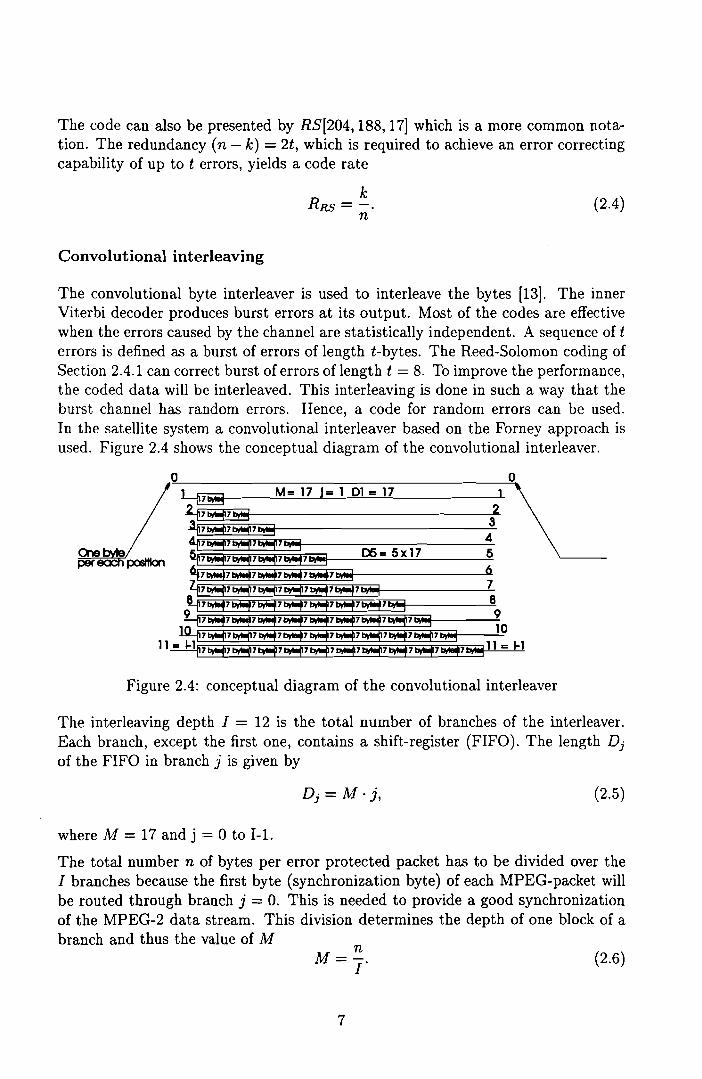
The convolutional byte interleaver is used to interleave the bytes [13]. The innerViterbi decoder produces burst errors at its output. Most of the codes are effectivewhen the errors caused by the channel are statistically independent. A sequence of terrors is defined as a burst of errors of length t-bytes. The Reed-Solomon coding ofSection 2.4.1 can correct burst of errors of length t = 8. To improve the performance,the coded data will be interleaved. This interleaving is done in such a way that theburst channel has random errors. Hence, a code for random errors can be used.In the satellite system a convolutional interleaver based on the Forney approach isused. Figure 2.4 shows the conceptual diagram of the convolutional interleaver.

o 0~ M= 17 J= 1 Dl = 17 1

~7~7Î,îiïil 2.ajl7~7t'ïij7b1îiïil 34jï7~7~7~7b1ÏÏij 45jï7ÏJ,tîï~ï7~7~7Ïîw"'7 b/ïîîïI D5 =5 x 17 56i7îJitïij7Î:;;tïïI7Î,~ 7tiWi8ïtn,ïïïIï7b7iWI 6Zp~7~7~7~7 b!îî17 î7iïïïp bjÎÎÎÎj 7~7~7~7~7~7~7~7~7b1ÏÏij 8~-Pî7itïîl7~7~7~7~7~7î7iîîîl1î7~7t>,4ïîj 9

1O....j17Ï.iïï1Ï7Ï.itïf7 b!îî17 bOJïïïf 7tÎwïïïïjî7t7"P tlïiî3l7tî~îï1i7Ï7iïiïï(ï7 blîiïil 10

11 = I-lp7~7~7~7~7~7ïî\ïiïî4î7Ï7iïiïï(ï7î7iïïïïjî7~7~7t>,4ïîj 11 = 1-1

Figure 2.4: conceptual diagram of the convolutional interleaver

The interleaving depth I = 12 is the total number of branches of the interleaver.Each branch, except the first one, contains a shift-register (FIFO). The length Djof the FIFO in branch j is given by

Dj = M'i, (2.5)

(2.6)n

M=T

where M = 17 and j = 0 to 1-1.

The total number n of bytes per error protected packet has to be divided over theI branches because the first byte (synchronization byte) of each MPEG-packet willbe routed through branch i = O. This is needed to provide a good synchronizationof the MPEG-2 data stream. This division determines the depth of one block of abranch and thus the value of M

7

For the satellite system with n = 204 bytes and I = 12, M equals 17. The advantageof a convolutional interleaver with respect to a block structured interleaver is thatit better matches for use with the class of convolutional codes [30]. The satellitesystem uses a convolutional coder.

Convolutional code

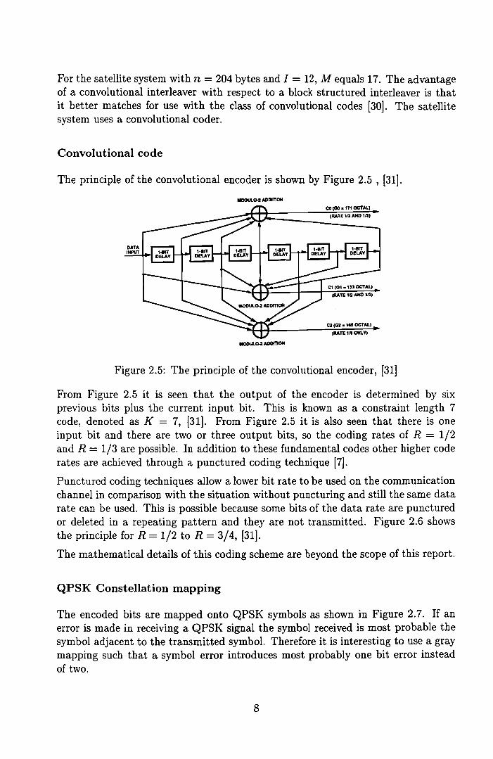
The principle of the convolutional encoder is shown by Figure 2.5 , [31].

DATAINPUT

co (00.171 OCTAl)

(RATE 112 ANC ''''

C2 (02 • 115 OCTALl

IRAn '" 0tlI.Y1

Figure 2.5: The principle of the convolutional encoder, [31]

From Figure 2.5 it is seen that the output of the encoder is determined by sixprevious bits plus the current input bit. This is known as a constraint length 7code, denoted as K = 7, [31]. From Figure 2.5 it is also seen that there is oneinput bit and there are two or three output bits, sa the coding rates of R = 1/2and R = 1/3 are possible. In addition to these fundamental codes other higher coderates are achieved through a punctured coding technique [7].

Punctured coding techniques allow a lower bit rate to be used on the communicationchannel in comparison with the situation without puncturing and still the same datarate can be used. This is possible because some bits of the data rate are puncturedor deleted in a repeating pattern and they are not transmitted. Figure 2.6 showsthe principle for R = 1/2 to R = 3/4, [31].

The mathematical details of this coding scheme are beyond the scope of this report.

QPSK Constel1ation mapping

The encoded bits are mapped onto QPSK symbols as shown in Figure 2.7. If anerror is made in receiving a QPSK signal the symbol received is most probable thesymbol adjacent to the transmitted symbol. Therefore it is interesting to use a graymapping such that a symbol error introduces most probably one bit error insteadof two.

8

DATAINPUT

0T~ "ECDV/NQ

STATION STA7ION

01 lICl) I D(2) ll(2) lI(4) lICs) I D(I)

@ fiH ëtIi? FiH ë;:r;i<9 I

011(1) Cll(1l I ClI(4) CO(I) ICHAHNELC111) C1121 C1f41 C1fl) Q-

G> I l1li(11 6- RlI(2)

IRO(4) -& RO(I)

Al(11 AI(2) :e: A1(4) A1(S) e:

<Y lIC·, D(2) lI(3) lI(4) Dis) lICI)

-e. NULL S'tMIIOL 1_11:

X. SYllBOL DELETED ('UNCTUAEt

Figure 2.6: The principle of puncturing [31]

The axes of this constellation are represented by the in phase modulation carriercomponent land the Quadrature modulation carrier component Q. Figure 2.7 showsa QPSK constellation.

IQ10

•

IQ11

•

QIQ00

•

I

Figure 2.7: A QPSK constellation diagram

In a QPSK there is always the 1r/2 phase ambiguity. The demodulator does notknow which symbol is received. It is possible however to detect the phase differencebetween the previous received symbol and the current received symbol. One way touse a QPSK link is thus to differentially encode the bits.

9

Differential encoding however decreases the performance of the link. If one symbol isreceived incorrect the result of the differential decoding is that two adjacent symbolsare decoded incorrect. This is because· the information is in the phase differencerather than in the phase itself.

The probability of a symbol error versus the carrier to noise ratio is shown in Figure2.8. The exact derivation of this figure will be given in Section 5.1.2.

Probability of a symbol error

0,0001

1e-06

1e-OB

x10 12 Eb 14__16~

No )

Figure 2.8: Probability of error versus carrier to noise ratio

From this Figure one can see that for links using high power, large carrier to noiseratios, the fact that the errors come in pairs and thus the probability of an error is

10

increased is no problem. The extra power required is negligible. For power restrictedsystems, low carrier to noise ratio, this effect is more severe as can be seen fromFigure 2.8. The required increase in the carrier to noise ratio due to the differentialencoding is then considerable. The exact relation between the probability of errorand the carrier to noise ratio will be discussed in Section 5.1.2.

The MVDS system is to be operated at 42 GHz. Since it is difficult to build anpower amplifier at these high frequencies the MVDS system is a power restrictedsystem. The differential coding is thus not very interesting for an MVDS system.

The phase ambiguity has thus to be solved in a different way for instance using aunique pattern in the transmitted sequence. The correct phase can be selected on thereception of this pattern [18]. Another simple method is to look at the performanceof the different decoding algorithms (Viterbi, Reed Solomon). If the performancewith the current phase assumption isn't adequate a different phase can be assumed.The total synchronization time will increase with this method of synchronization.It is therefore very interesting to detect an erroneous phase assumption in the veryfirst parts of the decoding e.g. the Viterbi decoder. There are of course numerousother techniques of solving the phase problem. A more detailed discussion is not inthe scope of this report.

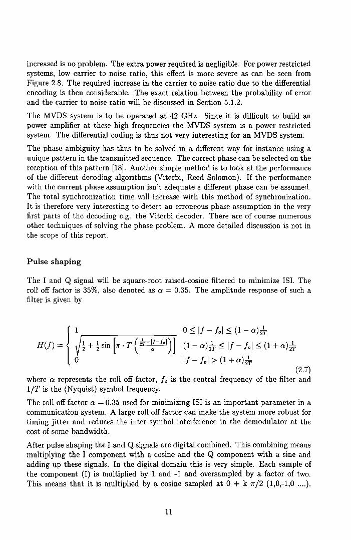
Pulse shaping

The land Q signal will be square-root raised-cosine filtered to minimize IS!. TheroIl off factor is 35%, also denoted as a = 0.35. The amplitude response of such afilter is given by

o~ If - fol ~ (1 - a) A(1 - a) 2~ ~ If - fa I~ (1 + a) 2~

If - fol > (1 + a)2~(2.7)

where arepresents the roU off factor, fa is the central frequency of the filter andI/T is the (Nyquist) symbol frequency.

The roU off factor a = 0.35 used for minimizing ISI is an important parameter in acommunication system. A large roU off factor can make the system more robust fortiming jitter and reduces the inter symbol interference in the demodulator at thecost of some bandwidth.

After pulse shaping the land Q signals are digital combined. This combining meansmultiplying the 1 component with a cosine and the Q component with a sine andadding up these signais. In the digital domain this is very simpie. Each sample ofthe component (I) is multiplied by 1 and -1 and oversampled by a factor of two.This means that it is multiplied by a cosine sampled at 0 + k 7r/2 (1,0,-1,0 .... ).

11

If the other component (Q) is treated the same but the result is shifted over onesample it is in fact multiplied with a sine sampled at °+ k 1r/2 (1,0,-1,0 .... ). Ifthese samples are added up the result is a QPSK modulated carrier in the digitaldomain.

Transmitter front end

The input of the transmitter front-end is the digital signal from the pulse shaper/ combiner.First the fundamental interval is filtered out from the digital information and thesignal is converted to an analog signal. The next step is to transpose the signal tothe L-band frequency. From the L-band the signal must be up-converted to the RFfrequency of 42 GHz in one or more steps. In the last step the signal is amplifiedand fed to the transmitter antenna.

This description is of course a simplified and a theoretical description of the realsituation (direct up conversion). The practical method of up conversion is morecomplex and technology dependent. A main problem of direct up conversion is thelinear amplification at 42 GHz. It is very difficult to generate power at these highfrequencies using linear amplifiers.

Another method is using a non-lïnear device to double or triple the frequency afterit has been amplified at a lower frequencies. This is a very common method whenanalog FM modulation is used. For QPSK modulation this method is not idealsince it introduces ISI even without noise and with perfect Nyquist filters. Theamount of ISI depends on the nyquist filters used. Since the MVDS must complyto the satellite standard the Nyquist filters can not be changed. This means thatthis method is not usabie. A third method is to mix the L-band source signal to anintermediate frequency of 14.5 GHz. At this frequency linear power amplifiers canbe used. An oscillator generates a frequency of 13 GHz. This can be amplified anddoubled by a not linear device since it is only a carrier. Then it is possible to mixthe 26 GHz power signa! and the 14.5 GHz power signal by means of a power mixerto the 40.5 GHz. The last step involves filtering and feeding it to the transmitterantenna. On all the schemes a back-off in the transmitter amplifier must be used ofcourse to guarantee linearity.

There are other scenarios possible. The best practical solution has to be furtherexamined and is not in the scope of this report.

2.4.2 Receiver description

Low noise block converter (LNB)

The low noise block converter LNB converts the 42 GHz RF signal to the L-bandsignal. From that point the standard digital satellite receiver can be used. The LNBconsists in principle of a band pass filter, low noise amplifier, local oscillator, mixer

12

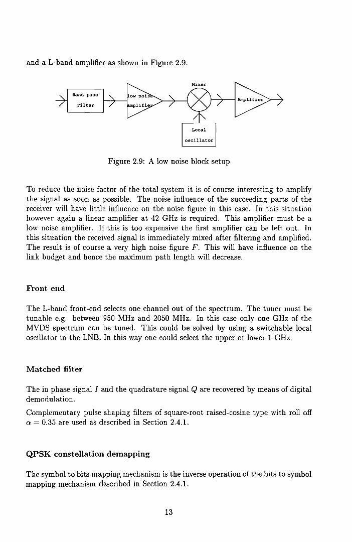
and a L-band amplifier as shown in Figure 2.9.

Band pass

Filter

Local

oscillator

Figure 2.9: A low noise block setup

To reduce the noise factor of the total system it is of course interesting to amplifythe signal as soon as possible. The noise influence of the succeeding parts of thereceiver will have little influence on the noise figure in this case. In this situationhowever again a linear amplifier at 42 GHz is required. This amplifier must be alow noise amplifier. If this is too expensive the first amplifier can be left out. Inthis situation the received signal is immediately mixed after filtering and amplified.The result is of course a very high noise figure F. This will have influence on thelink budget and hence the maximum path length will decrease.

Front end

The L-band front-end selects one channel out of the spectrum. The tuner must betunable e.g. between 950 MHz and 2050 MHz. In this case only one GHz of theMVDS spectrum can he tuned. This could be solved by using a switchable localoscillator in the LNB. In this way one could select the upper or lower 1 GHz.

Matched filter

The in phase signal land the quadrature signal Q are recovered by means of digitaldemodulation.

Complementary pulse shaping filters of square-root raised-cosine type with roIl off(X = 0.35 are used as described in Section 2.4.1.

QPSK constellation demapping

The symbol to bits mapping mechanism is the inverse operation of the bits to symbolmapping mechanism described in Section 2.4.1.

13

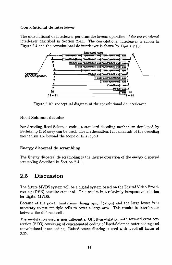
Convolutional de interleaver

The canvalutional de interleaver performs the inverse operation of the canvolutionalinterleaver described in Section 2.4.1. The convolutional interleaver is shown inFigure 2.4 and the convolutional de interleaver is shown by Figure 2.10.

Figure 2.10: conceptual diagram of the convolutional de interleaver

Reed-Solomon decoder

For decoding Reed-Salomon codes, a standard decoding mechanism developed byBerlekamp & Massey can be used. The mathematical fundamentals of the decodingmechanism are beyond the scope of this report.

Energy dispersal de scrambling

The Energy dispersal de scrambling is the inverse operation of the energy dispersalscrambling described in Section 2.4.1.

2.5 Discussion

The future MVDS system will be a digital system based on the Digital Video Broad­casting (DVB) satellite standard. This results in a relatively inexpensive solutionfar digital MVDS.

Because of the power limitations (linear amplification) and the large losses it isnecessary to use multiple ceUs to cover a large area. This results in interferencebetween the different ceUs.

The modulation used is non differential QPSK-modulation with forward error cor­rection (FEe) consisting of concatenated coding of Reed-Solomon outer coding andconvolutional inner cading. Raised-cosine filtering is used with a roU-off factor of0.35.

14

Chapter 3

Propagation aspects

In this Chapter we shall consider different propagation aspects, as discussed byFreeman [15], relevant for calculating the link budget in Chapter 5. This Chapteris based on [39J with some modifications.

3.1 Free space

The first step in looking at propagation is to calculate the free space 10ss L b/ whichoccurs in an idealized situation, this means an infinite empty space where the me­dium is assumed to be a vacuum.

We start with defining the transmitting antenna as an isotropic source in vacuum.We consider the envelope surrounding the antenna to be a sphere and the totalpower is Pt. The net power flux density Sav through a part of the surface of 1 squaremeter of the sphere with radius d equals

PtSav = 47rd2

(3.1)

where d is the distance.

An isotropic receiver antenna at distance d from the transmitting antenna will absorbpower which is equal to j3·sav where j3 is the effective aperture. The effective aperturefor an isotropic antenna is given by >.2/(47r) where >. is the wavelength [2]. The totalreceived power becomes

(3.2)

The loss is defined as

or

l _ Pt _ (47rd)2bI - - - -

Pr >.

( )

2Pt 47rd

Lb/.dB = lülog(p) = lülog T

15

(3.3)

(3.4)

3.2 Refractivity

In this section it is assumed that the radio beam is an infinite thin line in order tosimplify calculations. However in section 3.3 it will be shown that the actual radiopath is not a thin line.

In free space the path of a radio beam follows a straight line. In the earths at­mosphere however this is not always the case. This is due to the variation in therefractivity index n in the atmosphere. The refractivity index is defined as follows[151

cn= =~

Vmedium(3.5)

where the relative magnetic permeability Jlr = 1 in the atmosphere, €r is the relativeelectric permittivity, c is the velocity of light in vacuum and Vmedium is the velocityof the electromagnetic waves in the medium.

The refractivity index n ~ 1.003. The refractivity N is defined as

N = (n - 1) . 106 (3.6)

For radio frequencies the following relation holds (CCIR recommendation 453-2 [22]):

77.6 ( e)N = T P + 4810 . T

whereP = atmospheric pressure in millibarT = temperature in Kelvine = water vapor pressure in millibar77.6 = constant with dimension Kjmillibar4810 = constant with dimension K.

(3.7)

The error in this relation is less than 0.5% for frequencies up to 100 GHz. For asmall temperature deviation l:i.T, a small pressure deviation l:i.P and a small watervapour pressure deviation l:i.e we obtain the refractivity deviation. [2]

l:i.N = -1.12l:i.T + 0.268l:i.P +4.44l:i.e

where the ground level values for the Netherlands areTo = 290Po = 1026 mbareo = 11.4 mbarNo= 325.

16

(3.8)

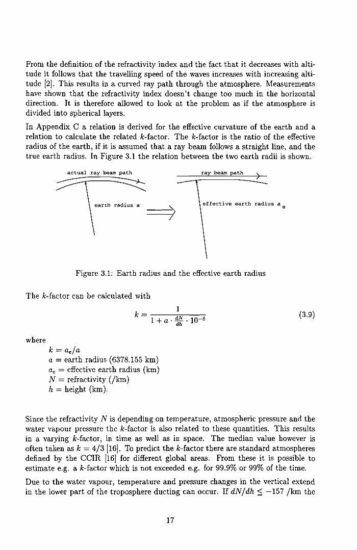
From the definition of the refractivity index and the fact that it decreases with alti­tude it follows that the travelling speed of the waves increases with increasing alti­tude [2]. This results in a curved ray path through the atmosphere. Measurementshave shown that the refractivity index doesn't change too much in the horizontaldirection. It is therefore allowed to look at the problem as if the atmosphere isdivided into spherical layers.

In Appendix Carelation is derived for the effective curvature of the earth and arelation to calculate the related k-factor. The k-factor is the ratio of the effectiveradius of the earth, if it is assumed that a ray beam follows a straight line, and thetrue earth radius. In Figure 3.1 the relation between the two earth radii is shown.

effective earth radius ae

actual ray beam path

~

earth radius a

ray beam path )

Figure 3.1: Earth radius and the effective earth radius

The k-factor can be calculated with

k = 11 + a . dN • 10-6

dh

wherek = ae/aa = earth radius (6378.155 km)ae = effective earth radius (km)N = refractivity (/km)h = height (km).

(3.9)

Since the refractivity N is depending on temperature, atmospheric pressure and thewater vapour pressure the k-factor is also related to these quantities. This resultsin a varying k-factor, in time as well as in space. The median value however isoften taken as k = 4/3 [16]. To predict the k-factor there are standard atmospheresdefined by the CCIR [16] for different global areas. From these it is possible toestimate e.g. a k-factor which is not exceeded e.g. for 99.9% or 99% of the time.

Due to the water vapour, temperature and pressure changes in the vertical extendin the lower part of the troposphere ducting can occur. If dN/ dh :::; -157 /km the

17

k-factor becomes negative. This means that the electromagnetic rays transmittedparallel to the earths surface are bended towards the earths surface. If they arethen reflected on the earths surface we have a surface duet. The wave is no longera spherical wave and the formula for the free space loss can't be used. If sucha duet exists more power than expected can be received. If in the lowest partdN/ dh ~ -157 /km an elevated ducting layer can exist.

If this phenomena occurs in a network much more interference than expected maybe the result.

3.3 Diffraction

Diffraction of a radio wave occurs when there is an obstacle in the radio path which isrelatively large compared to the wavelength. The amount of loss due to obstructionis proportional to the area of the beam which is obstructed.

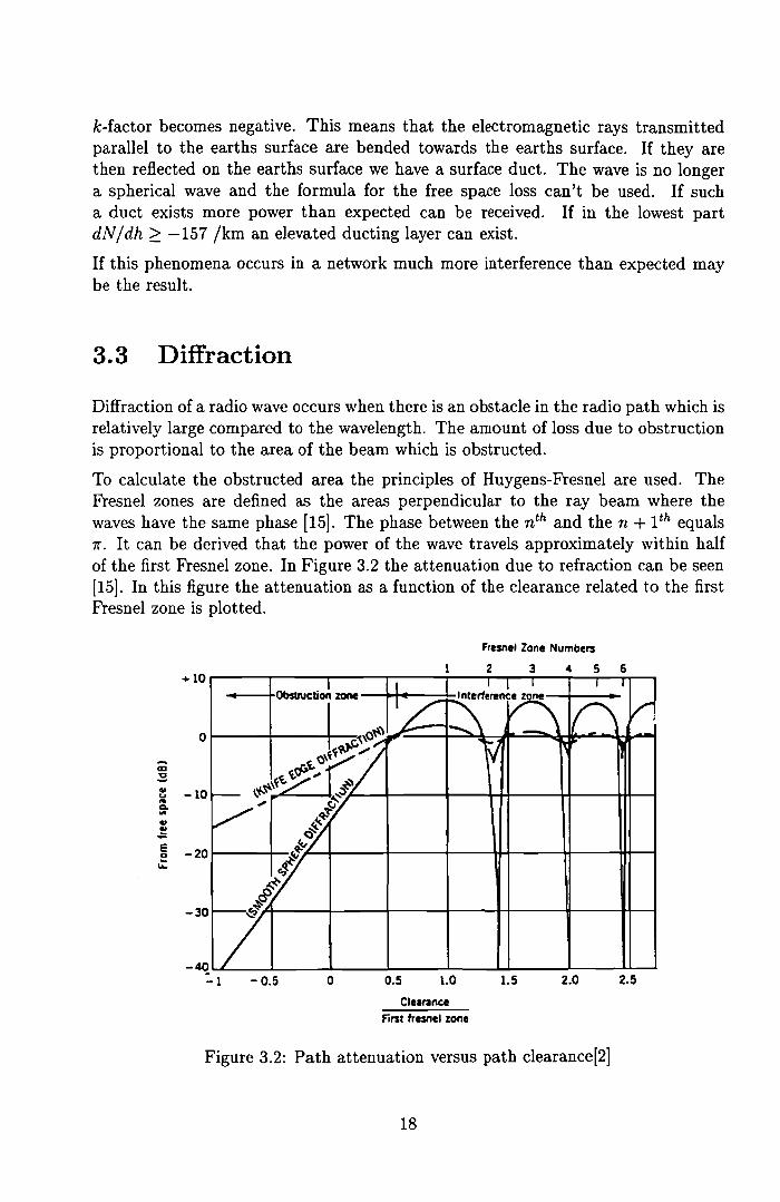
To calculate the obstructed area the principles of Huygens-Fresnel are used. TheFresnel zones are defined as the areas perpendicular to the ray beam where thewaves have the same phase [15]. The phase between the nth and the n + 1th equals7r. It can be derived that the power of the wave travels approximately within halfof the first Fresnel zone. In Figure 3.2 the attenuation due to refraction can be seen[15]. In this figure the attenuation as a function of the clearance related to the firstFresnel zone is plotted.

Fresnel Zone Numbers

Obst/uctioA zone I I I I f I

HI/,:::se~~~ n~"~ ......... -c.~\~"- 'tV

,.

~"7~~r;P~,~~\~~ f'.

r--II ~, ~V ~"f

~~~4

~~

1

4 5 6+10

o

~ -10...Slo..~

~ -20.::

-30

-~-1 - 0.5 o 0.5 1.0

2

1.5

3

2.0 2.5

Clearance

First tresnel zone

Figure 3.2: Path attenuation versus path clearance[2]

18

It is stated [15] that in the far field situation 0.6 times the first Fresnel zone clearancefrom obstruction of the beam edge is required to obtain an attenuation due to theobstacle of less than 3 dB.

The radius Rn of the nth Fresnel zone can be approximated with

(3.10)

whereRn = the radius of the nth Fresnel zone (m)dl and d2 are the distances from a point in the radio path to the antennas (km)f = the used frequency (Hz).

Providing a Fresnel zone clearance cl = 0.6 is sufficient to ensure that attenuationdue to an obstacle in or near the beam path is negligible [15]. It is however a verycommon use in microwave communications to use the foUowing clearance criteria(high reliability system):

cl ~ 0.3 . Rl at k = Icl ~ 1.0 . Rl at k = 3"'

If we take a look at the system at trial where the transmitter antenna height ht isapproximately 65 mand receiver antenna height hT is assumed to be 10 m we candraw the path of the ray beam (Figure 3.3). In this curve a coverage distance of 5km is assumed (the worst case will be at the edge of aceU). It is now possible tocalculate the minimum height of the first Fresnel zone along the path.

Receiver

Earth

Transmitter

(3.11)

Figure 3.3: Ray beam path and the first Fresnel zone

In figure 3.4 the height of the first Fresnel zone is plotted. In this figure a k-factorof -0.3, 4/3 and 0.3 is assumed. This height is given by

(h t - hT ) dl d2h(dd = dl + d

2• dl + hT - Rl (dd - 12.75. k

19

whereh is the height of the first Fresnel zonehr is the height of the receiver antenriaht is the height of the transmitter antennadl is the distance of the specific point to the receiverd2 is the distance of the specific point to the transmitterRl is the radius of the first Fresnel zone(d l d2 )/(12.75· k) is a correction for the earth curvature [15].

:[1:Dl"ijs:.Cl

~

) 30

"!!ii:

20

10

00 OoS 1.5 2 2.5 3

path length (km)3.5 4.5 5

Figure 3.4: The height of the first Fresnel zone (k=-0.3, 4/3 and 0.3)

From Figure 3.4 we can see that the extra clearance required for the fresnel zone forthis link is negligible. A line-of-sight between the transmitter and receiver will besufficient.

With this figure we can predict whether obstruction is a problem and if so whatantenna height will be necessary to overcome this problem. It obvious that for acity with high buildings a line-of-sight (LOS) with antennas on lower buildings isnot always possible. The number of possible reception sites will vary with differenteities and will be examined in Chapter 6.

3.4 Diffraction around obstacles

As we have seen in the previous section the bending of the waves due to the gradientin the refractivity index is negligible for the distances of concern. It is thus assumedthat the waves travel in a straight line.

This means that if the surface is fiat the total coverage area is illuminated withthe microwaves, no shadows. In an urban environment however there may be taU

20

buildings blocking the Line Of Sight (LOS). As can be seen from Figure 3.2 thereceived energy in a shadow area is not zero. Therefore it may be possible to havea good reception behind a tall building. This is very interesting because it willincrease the percentage of the coverage area where reception is possible in an urbanenvironment.

Since we are interested in the percentage of the coverage area where reception ispossible we are interested in the maximum angle of usabie diffraction. In Figure 3.5the coverage gain due to diffraction is illustrated.

;I;I;I Always Shaded

building

'\ '\ '\ Shaded LOS, not shaded if diffraetion ean be used

Figure 3.5: Coverage gain due to diffraction

It is thus necessary to have a close look at the diffraction problem. In Appendix D asimple analysis of a single knife edge diffraction is performed. The analysis assumeda infinitely long knife edge and line sources. The results from a single knife edge canbe very weIl used on rea! situations however. This is if we take the source to be apoint source and the knife edge to be longer than the width of the first Fresnel zoneif there where no obstruction. The radius of the First Fresnel zone is in our casealways smaller than 3.7 mand 3.0 m assuming a maximum distance to be coveredof 5 km and a frequency of respectively 28 and 42 GHz [39]. This theory can thusbe very weIl used on diffraction by large buildings.

The loss Ldf due to diffraction can be high for high frequencies however. As shownin Appendix D the attenuation Ldf of a single knife edge Ldf is given by

L df = 20 *log (I~h. [~(1 + j) - (C(~) + j. S(~))] I)

21

(3.12)

where C(~) and S(~) are the Fresnel integrals defined as

and

fnll 7r

S(~) = sin( - . v2) dvo 2

The parameter ~ is defined as

(3.13)

(3.14)

2 1 1_.(-+-)À dl d2

(3.15)

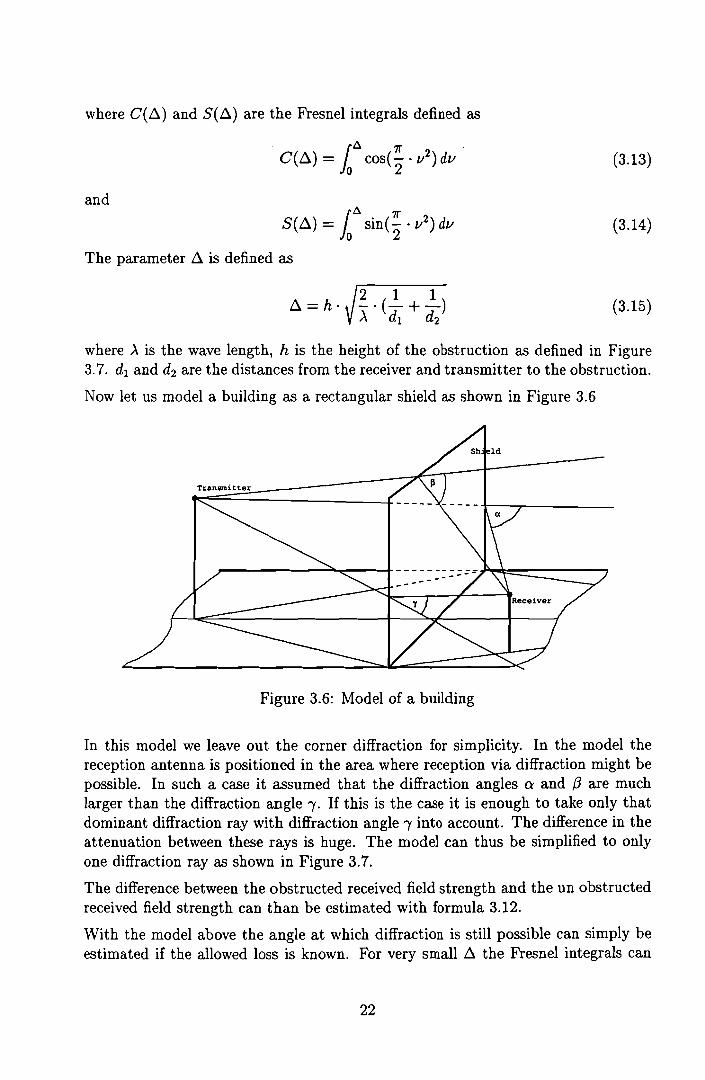
where À is the wave length, h is the height of the obstruction as defined in Figure3.7. dl and d2 are the distances from the receiver and transmitter to the obstructian.

Now let us model a building as a rectangular shield as shown in Figure 3.6

Figure 3.6: Model of a building

In this model we Ieave out the corner diffraction for simplicity. In the model thereception antenna is positioned in the area where reception via diffraction might bepossible. In such a case it assumed that the diffraction angles a and /3 are muchlarger than the diffraction angle 'Y. If this is the case it is enough to take only thatdominant diffraction ray with diffraetion angle 'Y into account. The difference in theattenuation between these rays is huge. The model ean thus be simplified to onlyane diffraction ray as shown in Figure 3.7.

The difference between the obstructed reeeived field strength and the un obstructedreceived field strength can than be estimated with farmuia 3.12.

With the model above the angle at whieh diffraction is still possible ean simply beestimated if the allowed loss is known. For very small ~ the Fresnel integrals ean

22

T R

Transmitterdl d2

Receiver

Figure 3.7: Diffraction simplified to one ray

be replaced by its series expansion.

C(~) = ~ + ~5 + ~9 + .S(~)=0+~3+~7+ .

(3.16)

(3.17)

Using the series expansion of the Fresnel integrals the attenuation due to diffractioncan be approximated for very smaU angles by [3]

Ldf = -6 - 8.7· ~ (3.18)

Formula 3.12 for estimating the attenuation can be approximated with the followingformulae

~ < -0.78 L df = OdB-0.78 < ~ < 0.8 Ldf = -6 - 8.7 . ~dB

(3.19)0.8 < ~ < 2.0 Ldf = -14 - 16 ·log(~)

2.0 < ~ Ldf = -13 - 20 ·log(~)

These formulae are simply fitted on the curve predicted by formula 3.12. Theseformulae can be very weU used for computing the attenuation. In Figure 3.8 theloss due to diffraction is given.

With the aid of these formulae the coverage gain due to diffraction can be calculatedif the dimensions of the buildings are known. As an example a the diffraction arounda large building will be calculated. Assume a building with the dimensions as shownin Figure 3.9

With the formulae above it is possible to predict the received field strength. Inthis example we assume the use of 28 GHz. The diffraction loss Lfd over the topof the building equals more than 40 dB, it is thus concluded that its contributionis negligible as stated before. To estimate the received field the diffraction aroundthe sides of the building is calculated. In Figure 3.10 the received field strength isshown as a function of x, where x is the distance to the optical shadow line in m.

23

-4

No obstructionAttenuation in dB

Obstruction

Figure 3.8: Attenuation due to diffraction

From this figure it ean be seen that reception by diffraction is not very usefu1 forMVDS at high frequencies. The attenuation at 42 GHz is even 1arger. For compar­ison the curves for 1 GHz, 28 GHz and 42 GHz are p10tted in Figure 3.10

In the 1 GHz examp1e the diffraction 10ss over the top of the building equa1s 26 dB.

24

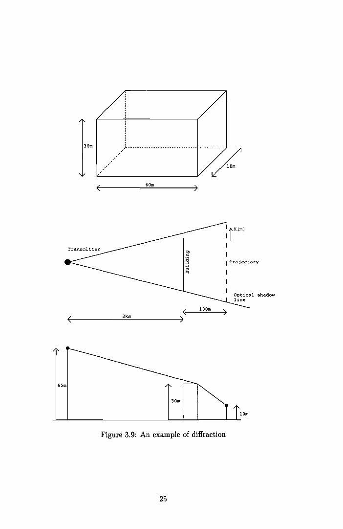
30m ,,////'" -- -- --- -_ -..~

( 60m )

I Trajeetory

shadow

)(~( ---=.:2km==---- ------})

lOm

Figure 3.9: An example of diffraction

25

Loss

-la

-15

-20

-25

-30

-35

o

(dB)

1 GHz

28 GHz

--4x

Figure 3.10: Diffraction 1088 around a building

26

lam

3.5 Reflections

In this section the reflection of incident waves on a surface is discussed. If elec­tromagnetic waves can be refiected on a surface, then such a refiection might beusabie for an MVDS system to increase the percentage of coverage. In Figure 3.11a configuration is shown how the percentage of possible coverage can be increaseddue to a refiection.

Receiver

.'l

l

..,:/

:~ ..'

l

..............

Transmitter

Figure 3.11: Increase in coverage due to one single refiection

If reception by means of a refiection is an interesting feature for MVDS depends onthe nature of the refiection and the nature of the environment, urban suburban etc.In the following sections a surface refiection is further examined.

In the first approach it is assumed that the ray beams obey the rules of opticalreBection e.g. no refraction.

In Figure 3.12 there is a model which uses two rays. In this figure kt is the transmitterantenna height, k r is the receiver antenna height and d is the distance betweentransmitter and receiver.

The field strength E at the receiver antenna consists of a contribution of the directwave and the reBected wave.

(3.20)

whereEo = direct wave field strengthp = refiection coefficient'I/J = phase difference due to path length difference.

27

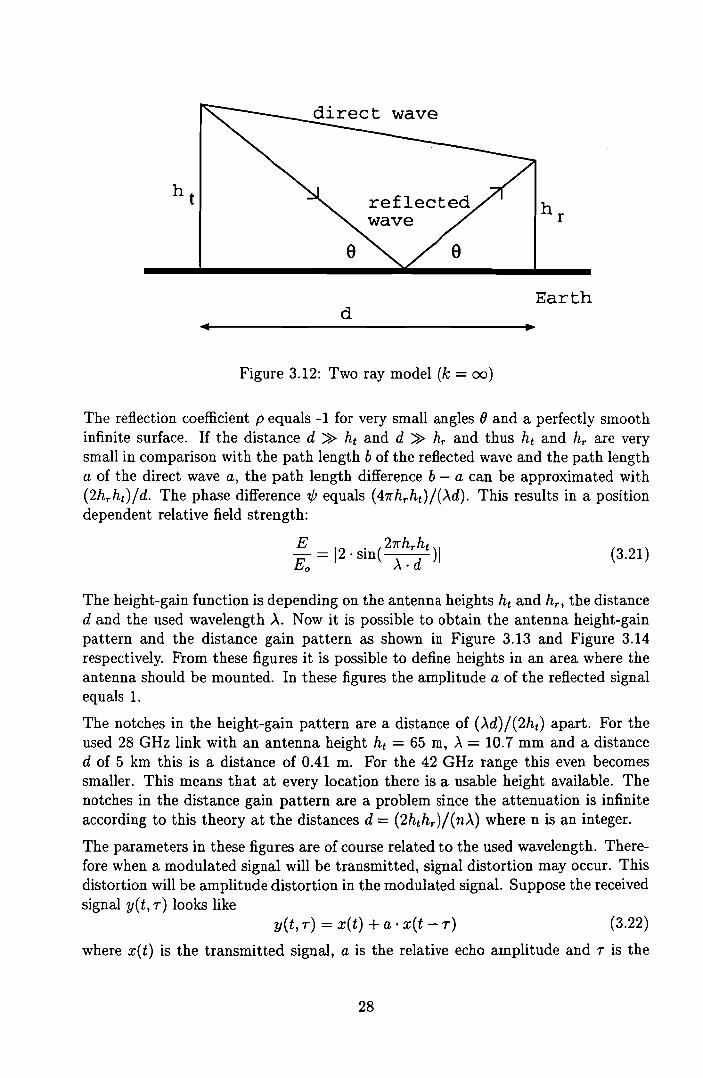
Earthd

Figure 3.12: Two ray model (k = 00)

The reflection coefficient p equals -1 for very small angles 0 and a perfectly smoothinfinite surface. If the distance d » ht and d » hr and thus ht and hr are verysmall in comparison with the path length b of the reflected wave and the path lengtha of the direct wave a, the path length difference b - a can he approximated with(2hr ht )/d. The phase difference 'I/J equals (47rhr ht )/()"d). This results in a positiondependent relative field strength:

(3.21)

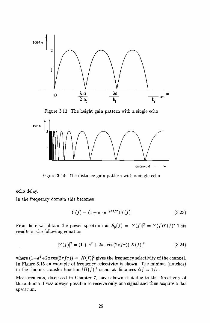
The height-gain function is depending on the antenna heights ht and hr , the distanced and the used wavelength )... Now it is possihle to ohtain the antenna height-gainpattern and the distance gain pattern as shown in Figure 3.13 and Figure 3.14respectively. From these figures it is possihle to define heights in an area where theantenna should he mounted. In these figures the amplitude a of the reflected signalequals 1.

The notches in the height-gain pattern are a distance of ()"d)/(2h t ) apart. For theused 28 GHz link with an antenna height ht = 65 m, ).. = 10.7 mm and a distanced of 5 km this is a distance of 0.41 m. For the 42 GHz range this even hecomessmaller. This means that at every location there is a usahle height availahle. Thenotches in the distance gain pattern are a prohlem since the attenuation is infiniteaccording to this theory at the distances d = (2h thr }/(n)..) where n is an integer.

The parameters in these figures are of course related to the used wavelength. There­fore when a modulated signal will he transmitted, signal distortion may occur. Thisdistortion will he amplitude distortion in the modulated signal. Suppose the receivedsignal y(t, T) looks like

y(t, T) = x(t) + a· x(t - T) (3.22)

where x(t) is the transmitted signal, a is the relative echo amplitude and T is the

28

m

Figure 3.13: The height gain pattern with a single echo

distanced -

Figure 3.14: The distance gain pattern with a single echo

echo delay.

In the frequency domain this becomes

Y(J) = (1 + a . e-i21r!T)X(J) (3.23)

From here we obtain the power spectrum as Sy(J) = IY(J)12 = Y(J)Y(Jt Thisresults in the following equation

IY(J)1 2 = (1 + a2+ 2a . cos(271' fT))/X(J)1 2 (3.24)

where (1 +a2+2a cos(27l' fT)) = IH(J) 12 gives the frequency selectivity of the channel.

In Figure 3.15 an exarnple of frequency selectivity is shown. The minima (notches)in the channel transfer function IH(J)/2 occur at distances !:J.f = l/T.

Measurements, discussed in Chapter 7, have shown that due to the directivity ofthe antenna it was always possible to receive only one signal and thus acquire a fiatspectrum.

29

10

5

oSelectivity

10 ·log(IH(fW)-5

-10

-.....,. ~ ~ ~ /

\ I \ ! \ ! \ I\ ! \ I1 \ ! \ !

1

-1510 12 14 16

Frequency f18 20

Figure 3.15: Frequency selectivity 10 ·log(IH(fW) (a=l)

3.5.1 Fresnel refiection coefficients

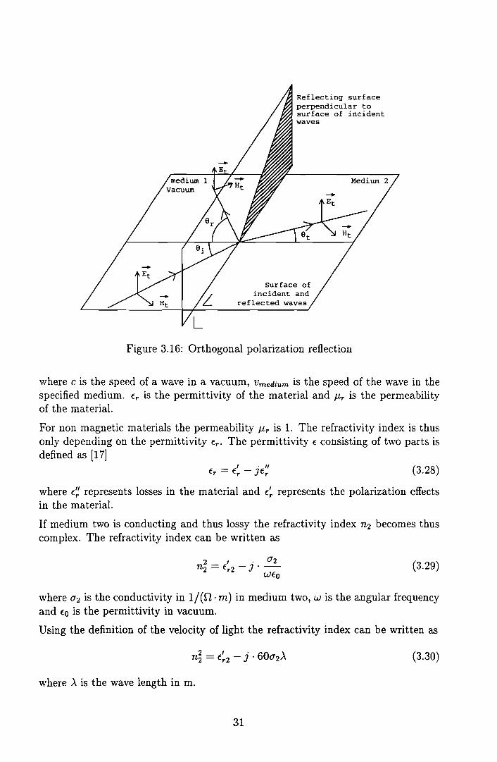
If electromagnetic waves refiect on a surface the waves can be decomposed into aparallel refiection and a orthogonal refiection. Orthogonal refiection means that thepolarization of the incident wave is orthogonal to the surface of incidence, parallelreflection obviously means the opposite where the polarization of the wave is parallelto the surface of incidence. In Figure 3.16 and Figure 3.17 the angle of arrival Oi isdefined and parallel and orthogonal refiection is depicted.

The Fresnel refiection coefficients for orthogonal and parallel refiection can be foundin numerous text books and are defined as

and

COS(Oi) _ (~)2 _ sin2(Oi)Pi. = ---~;=====;::====

COS(Oi) + (~)2 _ sin2(Oi)(3.25)

(3.26)

where the angle of incidence Oi is defined as shown in Figure 3.16 and nl and n2 arethe refractivity indexes in the two media. The refractivity index n is defined as

cn= =~

Vmedium

30

(3.27)

Reflecting surfaceperpendicular tosurface of incidentwaves

Surface ofincident and

reflected waves

Figure 3.16: Orthogonal polarization refiection

where c is the speed of a wave in a vacuum, Vmedium is the speed of the wave in thespecified medium. f r is the permittivity of the material and J.1r is the permeabilityof the material.

For non magnetic materials the permeability J.1r is 1. The refractivity index is thusonly depending on the permittivity fr' The permittivity f consisting of two parts isdefined as [17]

(3.28)

where f~ represents losses in the material and f~ represents the polarization effectsin the material.

If medium two is conducting and thus lossy the refractivity index n2 becomes thuscomplex. The refractivity index ean be written as

(3.29)

where (J2 is the eonductivity in 1/(n· m) in medium two, w is the angular frequeneyand fO is the permittivity in vaeuum.

Using the definition of the velocity of light the refraetivity index ean be written as

(3.30)

where À is the wave length in m.

31

Reflecting surfaceperpendicular tosurface of incidentwaves

Surface ofincident and

reflected waves

Figure 3.17: Parallel polarization reflection

In literature the material parameters are often given as €r and the loss tangent tan(ó)with Ó the loss angle. These parameters can be converted with

and

( f:) €~ 60·Àatanv =-=---€~ €~

Thus the refractivity index can also be written as

n2 = €r - j . €r • tan(ó)

(3.31)

(3.32)

(3.33)

In table 3.1 some material parameters at 60 GHz are given [10].

Since the refractivity index becomes complex if the media is lossy the Fresnel reflec­tion coefficients also become complex. This results in a phase difference between theincident wave and the refiected wave. At this time the only interest is in the ratioof the amplitudes of the incident and the reflected signal. Therefore the amplitudeof the refiection coefficients Pi. and Pil is of interest and not its argument. With thegiven material parameters the reflection coefficient of the material can be calculated.

This simple model may result in errors if the material is only slightly lossy or relat­ively thin[24]. In such a case the attenuation within the material is very small andthus a different model must be used.

32

Material f.r tan(b) a [dB/cm]Stone 6.81 0.0401 5.73MarbIe 11.56 0.0067 1.25Aerated concrete 2.26 0.0449 3.70Concrete 6.14 0.0491 6.67Tiles 6.30 0.0568 7.81Glass 5.29 0.0480 6.05Acrylic glass 2.53 0.0119 1.03Plaster board 2.81 0.0164 1.51Wood 1.57 0.0614 4.22Wood (chipboard) 2.86 0.0556 5.15

Table 3.1: Estimated material characteristics [10]

3.5.2 Reflection model of thin layers

A better model for refiection on thin layers is shown in Figure 3.18

( d )

Figure 3.18: A refiection model of thin layers[10]

This model uses an infinite series of refiections inside the material. If we assumethe building material thickness of approximately 5 cm to 10 cm the attenuationwithin the building material will be that large at the frequencies of concern that thiscomplex model is overdone for this application. If however the refiection materialis e.g. un coated glass which is thin and has very little attenuation this model ispreferred.

33

The generalized refiection Pg coefficient is then given by [10]

pe-j2k.,ft;s • e-2cu • e-jkd sin(0·)P = P _ (1 _ p2) • . . l

9 1 - p2 • e-]2k.,ft;s • e-2as • e-]kd sin(Oi)

where the propagation constant k is defined as

a is the attenuation coefficient defined as

s is the path length inside the slab between the two surfaces given by

Is = '[=-====

1 _ sin2(8i)f r

(3.34)

(3.35)

(3.36)

(3.37)

and dis the path length difference on the slab of two consecutive departing refiectionsgiven by

d = 21Jsin~(8;) - 1

(3.38)

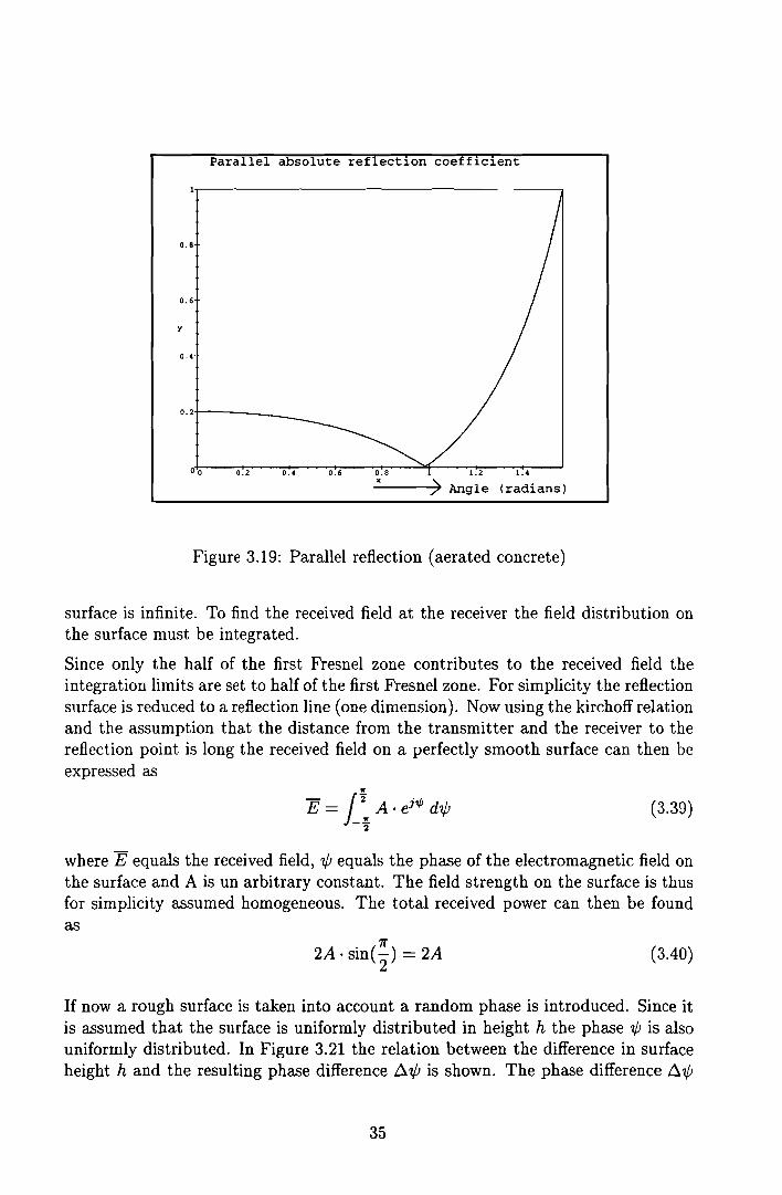
In Figure 3.19 and Figure 3.20 the absolute values of the refiection coefficients ofaerated concrete are given.

3.5.3 Reflection at rough surfaces

The measured refiection coefficients do not match these Fresnel refiection coefficients.This difference is assumed to be due to the roughness of the building material at highfrequencies. The refiection coefficients defined above assume coherent refiection. Ifelectromagnetic waves refiect on buildings this is not the case due to the very shortwavelengths and the roughness of the refiection surface. To illustrate the effect of arough surface on the amplitude of the refiection coefficient a simple model is used.This model is based on the assumption that the reflection surface can be modeledwith a large number of small squares which have a uniform height distributionbetween -h and h as depicted in Figure 3.21. This figure shows a refiection indetail.

The Fresnel zones are defined as the areas perpendicular to the ray beam wherethe waves have the same average phase [15]. The phase between the nth and then +1th equals 7r. It can be derived that the power of the wave travels approximatelywithin half of the first Fresnel zone [3]. If the refiection surface is very large so itencompasses the first Fresnel zone completely it can be assumed that the refiection

34

Parallel absolute ref ect~on eoe f~e~ent

1.4

(radians)0.8

"0.60.40.200

0.2t----__

0.8

0.4

y

0.6

Figure 3.19: Parallel refiection (aerated concrete)

surface is infinite. To find the received field at the receiver the field distribution onthe surface must be integrated.

Since only the half of the first Fresnel zone contributes to the received field theintegration limits are set to half of the first Fresnel zone. For simplicity the refiectionsurface is reduced to a refiection Hne (one dimension). Now using the kirchoff relationand the assumption that the distance from the transmitter and the receiver to therefiection point is long the received field on a perfectly smooth surface can then beexpressed as

E = i: A . eN d1/12

(3.39)

where E equals the received field, 'Ij; equals the phase of the electromagnetic field onthe surface and A is un arbitrary constant. The field strength on the surface is thusfor simplicity assumed homogeneous. The total received power can then be foundas

(3.40)

If now a rough surface is taken into account a random phase is introduced. Since itis assumed that the surface is uniformly distributed in height h the phase 1/1 is alsouniformly distributed. In Figure 3.21 the relation between the difference in surfaceheight hand the resulting phase difference b.'Ij; is shown. The phase difference ó.1/1

35

Orthogona absolute re lect~on coeff~c~ent

0.8

0.6

y

O••

0.2+-----

00 0.2 o.• 0.6 0.8 1.2 1..

---,,-x_)~ Angle (radians)

Figure 3.20: Orthogonal reflection (aerated concrete)

Figure 3.21: Non-coherent refl.ection detail

is given by211" 811" • h

6.'Ij; = T .6.8 = -À- . COS(Oi) (3.41)

The phase 'I/J thus f1.uctuates between 'I/J + 8 and 'Ij; - 8 where b is defined as

41r· h8 = -À- . COS(Oi) (3.42)

36

Assuming the above calculated homogeneous phase variation of [-ó, ó] the expecta­tion of the electromagnetic field < E > can be calculated as

< E >=< A !_: eN . d X >2

where x is the random variabie uniformly distributed from -ó to Ó.

The result from this integration is

< E >= 2A. < eix >

(3.43)

(3.44)

Now taking the expectation assuming that there is no dependence between adjacentsquares

this results in

_ !6. 1< E >= 2A· e}x. - dx-6 2ó

2A. sin(ó)Ó

(3.45)

(3.46)

It can now be concluded that if the Fresnel refiection coefficient on a perfectlysmooth surface is given by Po, the specular refiection coefficient on a rough surfacePs is given by

sin(ó)Ps = Po' -ó- (3.47)

From the formula above it can be seen that the refiection coefficient is reduceddramatically if the surface is rough. According to definition by Rayleigh a surfaceis smooth as

and rough as

À2h < . (0)8sm i

À2h > . (0)8sm i

(3.48)

(3.49)

According to our simple model this means if the specular refiection coefficient Ps issmaller than 0.9 the surface is defined as rough. In the simple model this meansthat Ó equals 1r/ 4 and 2h equals 1.34 mm if 28GHz is used and the angle of incidenceOi equals O.

A much more thorough and sophisticated analysis is done by P. Beckmann [4]. Inthis book a lot of models are used, a good model covered by P. Beckmann is basedon the assumption that the distribution is Gaussian. This leads to the followingresult for the specular refiection coefficient

{1 (41r'(J'COS(Oi))2}

Ps = Po . exp - '2 À

37

(3.50)

where ()i is the angle of incidence on the surface, À is the wave length and a is thevariance of the Gaussian distribution of the reflection surface height.

It is concluded that the reflection coefficients can only be found if the roughnessof the building material is known. The roughness of the building materials usedis not negligible. If the frequency of 42 GHz is used the influence of the surfaceof the building material increases and the reflection coefficient further reduces. InFigure 3.22 the specular refiection coefficient is shown for different surfaces. Fromthis figure one can see the effect of the surface roughness using aspecific frequency.

0.8

E

~0.6§

ioe~ 0.4ij8-(/)

02

1&+10"_(GHz)

1&+11

Figure 3.22: The specular reflection coefficient of rough surfaces

In Chapter 7 measurement results are shown and compared with this theory.

In theory the reflection coefficient becomes 1 if the angle of incidence ()i becomes7r/2, this is in a practical situation however not the case since the reflection surfacedoesn't encompass the first Fresnel zone anymore because it becomes infinite at suchan angle. The size of the Fresnel zone at grazing angle of incidence can be calculatedwith [4]

d (1 + 4~i~r)X n = -2 -'---""""'---:-""'2:­1 + (ht+hr)

n),d

(3.51)

where X n is the semi-major axis of the nth ellipsoid, ht is the transmitter antennaheight, hr is the receiver antenna height and d is the path length.

The semi-minor axis Yn can be calculated with

Jn>'dYn=--

2

38

( 1 + 4ht hr )n),d (3.52)

In table 3.2 some values of roughness [24], material parameters and refiection coef­ficients are given. These values were measured however at 60 GHz. The value Rinthis table is the value (down in dB) of the refiected field from the specific materialin comparison with a metal sheet.

Perpendicular polarization R (10°) -dB R (50°) -dB R (70°) -dBMaterial (thickness d [cm];estimated roughness (J [mm]Aerated concrete (5; 0.2) 14.1 9.6 5.1Concrete (5; 0.1) 7.5 5.3 2.0Briek (11; micro 0.3; macro 2) 14.8 12.3 4.8Glass rough (0.4; 0.3) 6.7 2.9 0.8Glass smooth (0.4; 0.0) 17.6 5.3 2.9Glass smooth (0.6; 0.0) 10.7 7.6 3.4Glass smooth (0.8; 0.0) 8.8 5.5 2.6

Table 3.2: Material refiection properties[24]

3.6 Power fading (flat fading)

Fading is defined as the time variation of the level, phase or polarization of thereceived signal. Power fading is a wide band or frequency non-selective form offading which can be a result of one of the following:

- obstruction of the propagation path (variation of k-factor)- antenna decoupling (variation of k-factor) (narrow-beam antennas)- partial refraction of elevated layers in the propagation path- the receiver or transmitter antenna in a ducting layer- precipitation in the propagation path (rain, snow, fog, clouds etc.)

The fading due to obstruction of the propagation path, variation of the k-factor,can be predicted with the statistics of the standard atmospheres. The solution is toadjust the antenna heights to make sure that the first Fresnel zone clearance is metin the worst case.

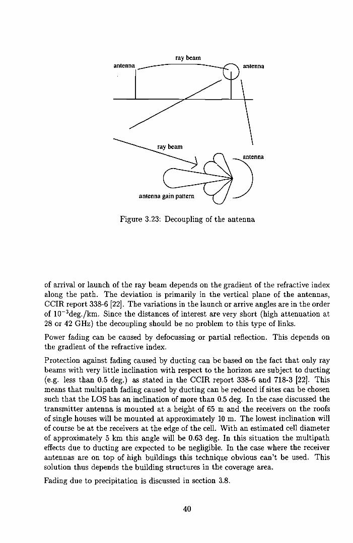
Antenna decoupling is the result of the bending of the ray beam in the troposphere.This can result in an incorrect angle of arrival of the transmitted power at theantenna as shown in Figure 3.23.

The amount of antenna decoupling depends on the antenna beam width. With highgain receiver antennas, narrow beam width, this can become aproblem. The angle

39

antennaray beam

antenna gain pattern

antenna

Figure 3.23: Decoupling of tbe antenna

of arrival or launeb of tbe ray beam depends on the gradient of tbe refractive indexalong tbe patb. The deviation is primarily in tbe vertical plane of tbe antennas,CCIR report 338-6 [22]. The variations in the launch or arrive angles are in tbe orderof 1O-3deg./km. Since the distances of interest are very sbort (bigh attenuation at28 or 42 GHz) tbe decoupling sbould be no problem to this type of links.

Power fading can be caused by defocussing or partial reflection. This depends onthe gradient of the refractive index.

Protection against fading caused by ducting can be based on tbe fact tbat only raybeams witb very little inclination with respect to tbe borizon are subject to ducting(e.g. less tban 0.5 deg.) as stated in tbe CCIR report 338-6 and 718-3 [22]. Thismeans tbat multipatb fading caused by ducting can be reduced if sites can be cbosensucb tbat the LOS bas an inclination of more tban 0.5 deg. In tbe case discussed tbetransmitter antenna is mounted at a beigbt of 65 mand tbe receivers on tbe roofsof single bouses will be mounted at approximately 10 m. The lowest inclination willof course be at tbe receivers at tbe edge of tbe cello Witb an estimated cell diameterof approximately 5 km this angle will be 0.63 deg. In tbis situation tbe multipatbeffects due to ducting are expected to be negligible. In tbe case wbere tbe receiverantennas are on top of high buildings tbis tecbnique obvious can't be used. Tbissolution tbus depends tbe building structures in the coverage area.

Fading due to precipitation is discussed in section 3.8.

40

(3.53)

3.7 Fading due to multipath propagation (frequencyselective fading)

We have seen in Section 3.5 that in theory multipath propagation can be verydramatic in the case of a strong single reflection. The multipath fading is frequencyselective as shown in Section 3.5. The reception of a secondary ray beam can bereduced if not eliminated with a very narrow beam width of the receiver antenna.This is of course depending on the attenuation by a reflection and the number ofreflections a ray beam makes before it reaches the receiver antenna and the pathlength difference. A disadvantage of this technique is that the antenna decouplingcan become a problem with very narrow-beam antennas. On this subject there hasto be thoroughly research done to make a good prediction. For such apredictionmodel very much data is required.

The statistics of fading caused by weak surface reflections are different from thosecaused by strong surface reflections. On a line-of-sight link there is no deep fadingexpected [16]. On these paths scintillation, slow non selective fading and more rapidfrequency selective fading is expected. Except for scintillation the fading is due tothe atmosphere forming ducts which is most likely to occur at night and early inthe morning in overland paths. Scintillation is less severe as the attenuation dueto precipitation using 42 GHz as will discussed in Section 3.5. Since scintillation isbased on stratified conditions which most probable do not exist if it is raining it isof no problem. The margin required in the link budget for the rain attenuation willprovide protection against scintillation.

If there is multipath reception the received signal consists of the direct line of sightsignal and a number of attenuated echoes. Such a channel is modeled by a Rice­Nagakami fading channel.

For large fade depths the average worst time fading time fraction can be approxim­ated with the following formula (CCIR report 338-6) [22, 161

W B CP(W) = K . Q . Wo . f . d

whered = distance (km)f = frequency (GHz)W = the received power (W)Wo = the unfaded received power (W)K . Q is a factor for different climate and terrain efIects.

This formula is considered valid for attenuations of more than 15 dB or the valueexceeded for 0.1%of the worst month for distances from 15 to 100 km. The constantsfor various circumstances can be found in table 3.7

41

Proposed or Jap.n N.W. Europe Umted kinJtdom nlte etate. USSR N orthern EuropeB: 1.2 1.0 0.85 1.0 1.5 1.0c: 3.~ 3.5 3.5 3.0 2.0 3.0K . Q for maritime temperate,mediterranean, coutal, orhigh humidity and

temperature dimatie region.: - - - ~ 2.10- 5s· -

K . Q for maritime eub-tropleal

dimatie region.: - - - ~s· - -K . C./ lor continenta' temperato

~c1imate. or mid latitude inland ;. to2

c1imatie regione with average 10-9 1.4.10-8~ 4.1.10-6 ~S' S'

~1 1

rolling terrain:S;;'

K . C./ for high dry

~mountainoue dimatie region.: 3.9. lO-10 . - 10-8S,

K . " for temperate chmatee,coaatal regione with fairly

ftat terrain: ~ 4.9· 10-5 ~- .1+ 2 S·

K . Q for temperate dimatea,inland regione with 7.6.10- 6 to

fairly ftat terrain - - - - 2. 10-5 ~S'

Table 3.3: Empirical values for formula 3.53[16]

Note: 11 1 and 112 are the antenna heighta in meters.SI ia the terrain roughneae meuured in meter. by the etandacd deviation of terrain elevatione at 1 km intervals (6 m :$ S1 ~ 42 m).S2 is defined aa the RMS va1ue of the .lapee (mrad) meaaured between pointe aepuated by 1 km along the path, but excluding thefir.t and the last complete km interval (1 IS2/ 80).Souree: CCIR report 338·6 [22J.

With this formula it is possible to prediet the attenuation due to multipath fading.In the link discussed however the distance is mueh shorter, the attenuation willtherefore be less, the formula is thus not applieable for our ealculation. If in futurethere will longer links (larger eel1 radii) this formula is preferabie.

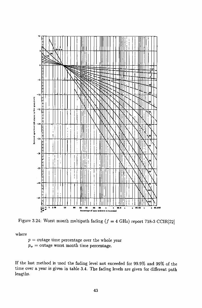
Another predietion method is based on the results of fitting a Rice-Nagakami dis­tribution to data measured over average rolling terrain in northwest of Europe [16](Figure 3.24). This method was developed for 4 GHz but it ean be used for other fre­quencies if the path length d is replaced by an equivalent path length deq calculatedwith the fol1owing formula [16]

(1)°·25deq = d· "4

whered = distance (km)deq = equivalent distance (km)1 = frequency (GHz).

(3.54)

This method also predicts the attenuation in the worst month of the year. Usingformula 3.55 [22] the outage time over a whole year can be calculated.

p = 0.3 . p~15 (3.55)

42

;; ~ I 510 !IO 110.0 t5 ti H • • H.'. • H.It. • tt.tli~ó· Puccnt.,e or lUM ordinale iA fXcetded

Figure 3.24: Worst month multipath fading Cf = 4 GHz) report 718-3 CCIR[22]

whereP = outage time percentage over the whole yearPw = outage worst month time percentage.

If the last method is used the fading level not exceeded for 99.9% and 99% of thetime over a year is given in table 3.4. The fading levels are given for different pathlengths.

43

Path length fading depth fading depth fading depth fading depth(km) 28 GHz 99 % (dB) 42 GHz 99.9% (dB) 28 GHz 99.9 % (dB) 42 GHz 99% (dB)

3 2.5 2.8 1.8 2.14 3.1 3.3 2.1 2.35 3.5 3.7 2.3 2.56 4.0 4.3 2.5 2.87 4.3 4.7 2.8 3.0

Table 3.4: Fading depth as a function of path length for 28 GHz and 42 GHz

The last method is based on smooth rolling terrain, therefore the prediction of thefading level for eities may be incorrect. For now this value is used but the statisticsof attenuation of a 28 GHz or 42 GHz signal due to multipath fading within eitieshas to be reviewed thoroughly. Measurements as described in Chapter 7 did notshow any fast or slow fading using the narrow-beam antenna.

3.8 Rain attenuation

Attenuation caused by rain plays a very important role in millimeter wave trans­mission. It has been recognized as one of the principal causes of attenuation inthe millimeter wave propagation [11]. Rain is not the only cause however, cloudswill also cause attenuation in the lower part of the atmosphere. In the case of theMVOS the signalloss due to the clouds is of less importance since we rely on a lineof sight transmission at 28 and 42 GHz and therefore the clouds do not intersect thepath. With the exceptions of the frequency bands about the 22 GHz water vapourabsorption line and the 60 GHz complex of oxygen lines, the attenuation exceededless than 2 percent of the year is caused by rain or clouds [11]. At the smallerpercentages rain is the only cause of increased attenuation.

Areliabie estimation of the attenuation by rain is therefore necessary to realisticallydetermine the link availability. If this signal loss is taken account for in the linkmargin the rain should not be a real problem. There are numerous models whichpredict the statistical behaviour of rain attenuation,

Very well known models are those of Rice-Holmberg [32], Lin [28], Crane [11] andthe CCIR model. The model used will be the CCIR model.

On terrestrial paths the CCIR model is one of the most accepted methods of es­timating the rain attenuation. The attenuation is speeified for both horizontal andvertical polarization. This is important for acellular network since this will prob­ably make use of the cross-polar discrimination of antennas. Such a system mustthen cope with the different cell sizes when the different polarizations are used.

The CCIR model has very small regions where the predicted attenuation would beconstant and thus has a very fine rain rate variations. The CCIR model is based bothon physics and on mathematical curve fitting on the attenuation measurements.

44

3.9 ITU-R rain model

The CCIR model to predict the attenuation by rain is based on the empirical ap­proximate relation between the specific attenuation "fT and the rain rate R [20].

(3.56)

where"fT = the specific attenuation (dB/km)R = rain rate (mm/hr)k and a are functions of frequency and rain temperature.

The values of k and a can be found in Table 3.5 [21]. Due to the shape of the raindrops (oblate spheroids) the attenuation in horizontal and vertical polarized wavesdiffer (Figure 3.25) [16, 12]. The horizontal polarized waves encounters the highestattenuation because in this plane there is relatively more water.

Movement

Vertical

Horizontal--+-----+------+--

Figure 3.25: Model of a falling rain drop without a vertical wind gradient [12]

To estimate the long term statistics of rain attenuation the following steps must betaken. First (3.56) is applied with the rain rate Ro.ol taken from Table 3.6 with helpof Figure 3.28, where Rom is the rain rate exceeded 0.01 % of the time. The nextstep is to calculate the effective path length using the reduction factor r [20].

1r = d (3.57)

1 + do

wherer = the reduction factord = the path length (km)do = 35 . exp(-0.015 . Ro.od.

45

Frequency (Ghz) kh k u ah au1 0.0000387 0.0000352 0.912 0.8802 0.000154 0.000138 0.963 0.9234 0.000650 0.000591 1.121 1.0756 0.00175 0.00155 1.308 1.2657 0.00301 0.00265 1.332 1.3128 0.00454 0.00395 1.327 1.31010 0.0101 0.00887 1.276 1.26412 0.0188 0.0168 1.217 1.20015 0.0367 0.0335 1.154 1.12820 0.0751 0.0691 1.099 1.06525 0.124 0.113 1.061 1.03030 0.187 0.167 1.021 1.00035 0.263 0.233 0.979 0.96340 0.350 0.310 0.939 0.92945 0.442 0.393 0.903 0.89750 0.536 0.479 0.873 0.86860 0.707 0.642 0.826 0.82470 0.851 0.784 0.793 0.79380 0.975 0.906 0.769 0.76990 1.06 0.999 0.753 0.754100 1.12 1.06 0.743 0.744120 1.18 1.13 0.731 0.732150 1.31 1.27 0.710 0.711200 1.45 1.42 0.689 0.690300 1.36 1.35 0.688 0.689400 1.32 1.31 0.683 0.684

Table 3.5: Coefficients for estimating specifi.c attenuation [21]

In calculating the effective path length with help of the reduction factor r a ho­mogeneous rain rate throughout the path is assumed. This is however unlikely tohappen. To compensate for this assumption the factor do is included. The higherthe rain rate Ro.ol the more local this will be and thus the effective path length isreduced.

In the last step the actual attenuation AO.Ol along the path is calculated.

AO.01 = fT • d . r (3.58)

(3.59)

where dis the path length in km.

If one is interested in other time percentages p in the range 0.001% to 1% the valuecan be corrected with formula 3.59 [20].

Ap = 0.12. p-[0.546+0.043.1og(p)]

AO.Ol

where Ap = the corrected attenuation.

In Figure 3.26 some attenuation curves are given to show the relation between theattenuation and the time percentage and in Figure 3.27 the attenuation is shown asa function of the distance for vertical and horizontal polarization in rainfall regionE.

The average annual percentage of time P exceeding a given attenuation level may bederived from the worst month percentage of time Pw by use of the following formula

46

0.1exceeded time percentage p (%)

0.01

~'"•

.s -GH"i1ÏCriióöta ::::..... ,. .......

~

,~,"" " . '

" ........~.

~,,

............,~

......... ..~..~: .. ~~, .. ,~. ., _. ,

: :, . :

:o0.001

10

50

60

20

40

Figure 3.26: Attenuation curves versus time percentage p %

2~.~;.~~~ .....

12

10

8

6

4

Vertical attenuation exceeded 0.1\"10 (42GHZ~· ...­HorizontaJ attenuation lixceeded 0.1\% 142GHz· -;-­

VerticaI attenuatiori exceeded 1\% 42GHz·~Horizontàl attenuatiorl exceeded 1\% 42GHz. +-.

.;. ..; ,.. ..; ...............•.;0;"""' .

65.554.53 3.5 4Palh lenglh d (km)

2.521.5

OL..-__"'---__...J..-__....L..__.......__---'-__----' '---__..L-__-'-__-'

1

Figure 3.27: Attenuation curves versus distance d in km

[20]

P = 0.3 . p~.15 (3.60)

47

Percentage of time ('70) A B C D E F G H J K L M N P1.0 1 3 1 2 2 4 5 120.3 1 2 3 5 3 4 7 4 13 6 7 11 15 340.1 2 3 5 8 6 8 12 10 20 12 15 22 35 650.03 5 6 9 13 12 15 20 18 28 23 33 40 65 1050.01 8 12 15 19 22 28 30 32 35 42 60 63 95 1450.003 14 21 26 29 41 54 45 55 45 70 105 95 140 2000.001 22 32 42 42 70 78 65 83 55 100 150 120 180 250

Table 3.6: Rain rate (mm/hr) (CCIR)[21]

3.10 Cross-polar discrimination

To make effective use of the available spectrum frequency reuse by means of ortho­gonal polarizations is an interesting feature. The isolation between the two ortho­gonal polarizations is limited however. First of all the antennas have a statie limitedcross-polarization discrimination. This can be better than 20 dB if required. Thecross-polar discrimination is however further decreased due to the precipitation suchas rain in the transmission medium.

Some of the transmitted energy in one polarization is received in the other polariz­ation and visa versa. This effect introduces a cross-polar interference in the channelusing the same frequency but the other polarization.

Before we examine the depolarization effects more closely some definitions are givenaccording to [12] in Figure 3.29.

In this figure the transmitted and received field are defined as:

• Exx is the received signal in the X-direction and transmitted in the X-direction

• Eyy is the received signal in the Y-direction and transmitted in the Y-direction

• Exy is the received signal in the X-direction and transmitted in the Y-direction

• Eyx is the received signal in the Y-direction and transmitted in the X-direction

The cross-polar discrimination XPDx in the x-direction is now defined as

XPDx = -20 log I~::I

and the cross-talk discrimination in the x-direction is defined as

XTDx = -20l0gl~::1

Far the other orientation y the same formulae holds

XPDy = -20 log I~::I

48

(3.61)

(3.62)

(3.63)

••tS-

P*---+-"'"'7-F7''--:::+-'ä~t-r~;;lJ-~-I----+----':=---I----+----l ...

t:---+--+---+-*t---t1,--,.lIit-=:....-+-.......,f--+~1Hlo·

.....-=:::.......-+--+---+~-tT-=w~~~~:::::.....+-.......,f---+--l JO•

.s·

..·.'=r:---.L.---I:':I·;---~..----:'~I·;---'-----:.::,·----l'----:llI~.--J--...J,.~

Figure 3.28: Rainfall regions for Europe and Africa [16]

and the cross-talk discrimination in the y-direction is defined as

XTDy = -2010gl~::1 (3.64)

Raindrops falling through the atmosphere take an oblate form as a result of the air

49

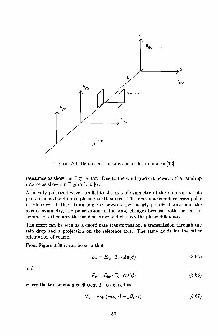
y

?- ~x

Figure 3.29: Definitions for cross-polar discrimination[12]

resistance as shown in Figure 3.25. Due to the wind gradient however the raindroprotates as shown in Figure 3.30 [6].

A linearly polarized wave parallel to the axis of symmetry of the raindrop has itsphase changed and its amplitude is attenuated. This does not introduce cross-polarinterference. If there is an angle a between the linearly polarized wave and theaxis of symmetry, the polarization of the wave changes because both the axis ofsymmetry attenuates the incident wave and changes the phase differently.

The effect can be seen as a coordinate transformation, a transmission through therain drop and a projection on the reference axis. The same holds for the otherorientation of course.

Prom Figure 3.30 it can be seen that

Eu = Eoy . Tu' sin((jJ)

andEv = Eoy • Tv . cos((jJ)

where the transmission coefficient Tu is defined as

Tu = exp (-au ·l - j(3u ·l)

50

(3.65)

(3.66)

(3.67)

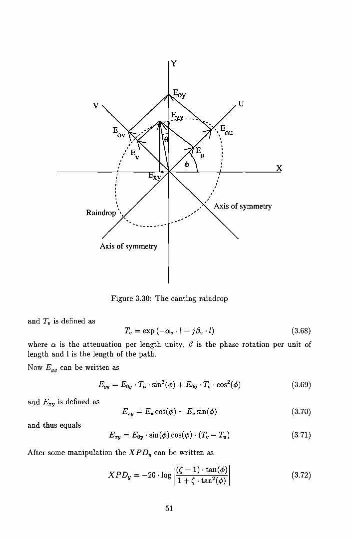
y

v

III,IIII,,

...... _-----_.

u

.... , '\ E'. ou,,

IIIIII,

Axis of symmetry

x

and Tv is defined as

Axis of symmetry

Figure 3.30: The canting raindrop

Tv = exp (-Gv 0 l - j /3v . l) (3.68)

where G is the attenuation per length unity, (3 is the phase rotation per unit oflength and I is the length of the path.

Now Eyy can he written as

and Exy is defined as

and thus equalsExy = Eoy 0 sin(4)) cos(4)) 0 (Tv - Tu)

After some manipulation the XPDy can he written as

XPD = _20 . log I( - 1) . tan(4>) Iy 1+(otan2 (4»

51

(3.69)

(3.70)

(3.71)

(3.72)

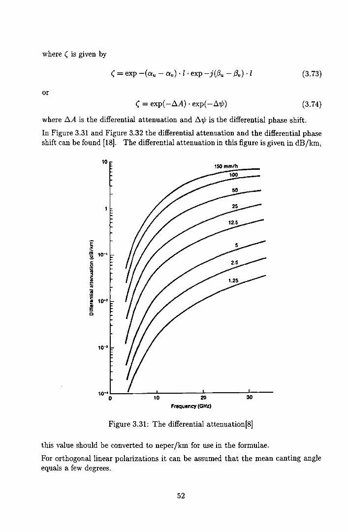
where ( is given by

or

(= exp(-~A) . exp(-~7/J)

(3.73)

(3.74)

where ~A is the differential attenuation and ~7/J is the differential phase shift.

In Figure 3.31 and Figure 3.32 the differential attenuation and the differential phaseshift can be found [18]. The differential attenuation in this figure is given in dB/km,

10

10-.L-_~__...J.... ~ --=~__o 10 20 30

Frequency (GHz)

Figure 3.31: The differential attenuation[8]

this value should he converted to neper/km for use in the formulae.

For orthogonallinear polarizations it can be assurned that the mean canting angleequals a few degrees.

52

100

150mm/h

10

Ê~....~:B.:::ë..Is:.Q.

:!ëeti

==0

10-1

10-1

L ...J.... ......1: --:':-__o 10 20 30

Frequency GHz)

Figure 3.32: The differential phase shift[8]

The ITU-R recommends (in recommendation 530-4) [23] the following simple semiempirical formula for system planning however

XPD = V(J) - V(J)log(CPA) (3.75)

where V(J) equals 9 + 30log(J), V(J) equals 20 and CPA is the co-polarized at­tenuation.

This formula will be used here because it has been proven to be accurate and is basedon both the theory above and is matched on data of extensive measurements. Thereare however few data in the 42 GHz band, according to the ITU-R this prediction isvalid up to 35 GHz. Future measurements should provide the data, with this dataone can check if the model is valid for these frequencies.

In our case the CPA just equals the rain attenuation. If the rain statistics of section3.8 are used the XPD exceeded for p % of the year can be calculated. The total

53

outage time does not necessarily increase because the worst cross-polar occurs mostprobably at the same time as the outage due to rain attenuation. Therefore it isbest to add degradation in dB's instead of adding up the outage- time.

As an example a path length of 5 km with rain is considered and the frequency is42 GHz. We are now interested in the lower XPD bound which is not exceeded for99 % of the time or 99.9 % of the time. From Section 3.8 it is found that the rainattenuation La not exceeded for these time percentages equals 3.38 dB and 10.76dB respectively (horizontal polarization).

The XPD found using the formulae above, assuming a homogeneous rain ratethroughout the entire path, equals 37.06 dB (99.9 %) and 47 dB (99 %). Thusthe XPD is better than 37 dB for 99.9 % of the time. It is thus concluded thatthe XPD will not be a serious problem, the attenuation due to the rain is muchmore of a problem to overcome. This means that the outage time of the link is notinfiuenced by the cross-talk between the two polarizations.

The analysis above does not mean that the total cross-polar discrimination is thatgood because the transmitter and receiver antennas both have a limited cross-polardiscrimination. In Chapter 7 the results of a cross-polar discrimination measurementare discussed.

The total cross-polar discrimination of a link will then be determined by the cross­polar discrimination of the antennas. The total cross-polar discrimination worstcase can be calculated with [18]

1 ( 1 )xpdt = - . 1 1

2 Xpdl + Xpd2

(3.76)

where xpdi = lOXPDi/lO

If for instance both antennas have a XPD of 20 dB, the total resulting XPD of thelink becomes 14 dB.

3.11 Sky noise temperature

(3.77)1 1

Tsky,rain = T sky . la + (1 - l) . Train

The sky noise temperature T ant at the antenna is also effected by rain, the antennanoise temperature can therefore depend on the rain rate. This is because the antennanoise temperature is depending on the sky noise temperature. If Train represents therain temperature which is usually taken to be 273 K and l = 1/9 = la is the rainattenuation, then the antenna noise temperature TaTlt,rain noise temperature can becalculated with

But since the elevation of the antenna is approximately 0 deg. this effect does notoccur since the antenna will always look at buildings, trees and ground refiections

54

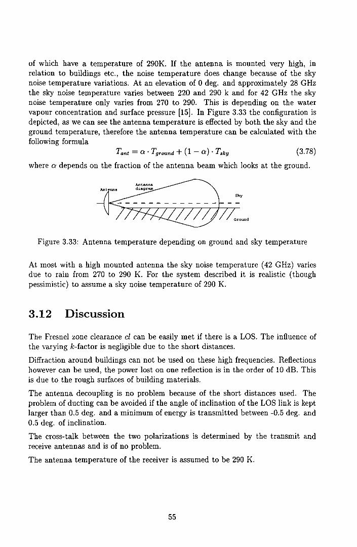
of which have a temperature of 290K. If the antenna is mounted very high, inrelation to buildings etc., the noise temperature does change because of the skynoise temperature variations. At an elevation of 0 deg. and approximately 28 GHzthe sky noise temperature varies between 220 and 290 k and for 42 GHz the skynoise temperature only varies from 270 to 290. This is depending on the watervapour concentration and surface pressure [15]. In Figure 3.33 the configuration isdepicted, as we can see the antenna temperature is effected by both the sky and theground temperature, therefore the antenna temperature can be calculated with thefollowing formula

Tant = a . Tground + (1 - a) . Tsky (3.78)

where a depends on the fraction of the antenna beam which looks at the ground.

Figure 3.33: Antenna temperature depending on ground and sky temperature

At most with a high mounted antenna the sky noise temperature (42 GHz) variesdue to rain from 270 to 290 K. For the system described it is realistic (thoughpessimistic) to assume a sky noise temperature of 290 K.

3.12 Discussion

The Fresnel zone clearance cl can be easily met if there is a LOS. The influence ofthe varying k-factor is negligible due to the short distances.

Diffraction around buildings can not be used on these high frequencies. Reflectionshowever can be used, the power lost on one refiection is in the order of 10 dB. Thisis due to the rough surfaces of building materiais.

The antenna decoupling is no problem because of the short distances used. Theproblem of ducting can be avoided if the angle of inclination of the LOS link is keptlarger than 0.5 deg. and a minimum of energy is transmitted between -0.5 deg. and0.5 deg. of inclination.

The cross-talk between the two polarizations is determined by the transmit andreceive antennas and is of no problem.

The antenna temperature of the receiver is assumed to be 290 K.

55

Chapter 4

Network topology

If the system parameters are known the coverage in a given area can be calculated.If we wish to cover a large area the area must be divided in smaller cells as shownin Figure 4.1 [34]. A simple but inefficient method is to use different frequencies forthe different cells.

Figure 4.1: Area serviced with multiple eeUs

The frequency reuse distance defined as the distanee where the same frequency canbe reused depends on a lot of parameters [9]. For the analog test system (28 GHz)it is shown in Appendix B that the power decay corresponds to the theoretical 1/d2

scenario where dis the distance. In Chapter 7 measurement results are shown whichshows that this is correct. It is assumed that the received power of a 42 GHz system

56

will also be proportional to 1/d2• This conclusion is based on the required LOS andAppendix B.

The ultimate situation is of course if in the adjacent cells the same frequency canbe used, such a network is known as a Single Frequency Network (SFN). In thefollowing sections the possibilities of frequency reuse in different cells are examined.

The directivity of the reception antennas used in microwave systems is very high.This is something which can be very well used in employing a frequency efficientcell structure [40].

The frequency reuse distance is determined by the amount of interference which istolerabIe. In Figure 4.2 the effect of interference from other transmitters on thereuse distance is shown.

Field frominterferer

Field from/ main transmitter

Fieldstrength

TolerabIe carrier to interferenceratio

ofoverage are~

(Reuse distance

Distance) d

)

Figure 4.2: Frequency reuse distance

4.1 Cellular systems using omni directional an­tennas

In many cellular networks the antennas used are of the omni directional type. Inour first approach we will examine the possibilities of such a network and examinethe interference. In Figure 4.3 a configuration of such a network is shown which willbe evaluated as an example.

57

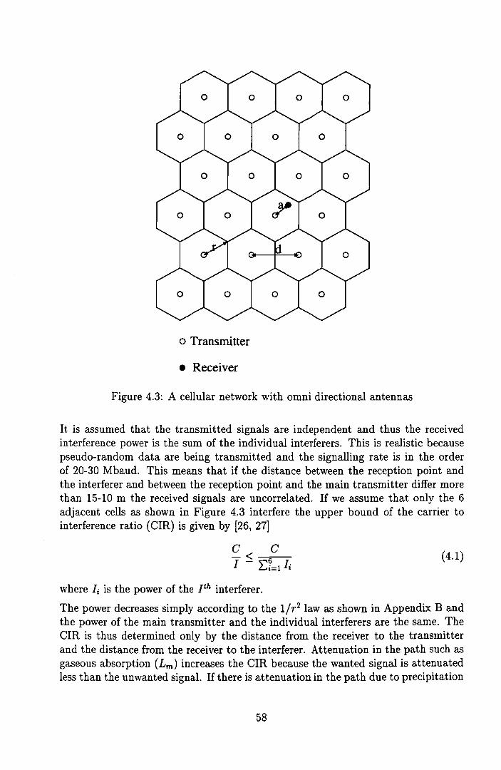
o Transmitter

• Receiver

Figure 4.3: Acellular network with omni directional antennas

It is assumed that the transmitted signals are independent and thus the receivedinterference power is the sum of the individual interferers. This is realistic becausepseudo-random data are being transmitted and the signalling rate is in the orderof 20-30 Mbaud. This means that if the distance between the reception point andthe interferer and between the reception point and the main transmitter differ morethan 15-10 m the received signals are uncorrelated. If we assume that only the 6adjacent ceUs as shown in Figure 4.3 interfere the upper bound of the carrier tointerference ratio (CIR) is given by [26, 27]

(4.1)

where I i is the power of the ph interferer.

The power decreases simply according to the 1/r2 law as shown in Appendix Bandthe power of the main transmitter and the individual interferers are the same. TheCIR is thus determined only by the distance from the receiver to the transmitterand the distance from the receiver to the interferer. Attenuation in the path such asgaseous absorption (Lm ) increases the CIR because the wanted signal is attenuatedless than the unwanted signal. If there is attenuation in the path due to precipitation

58

(4.3)

it is assumed that this attenuates both the wanted and the unwanted signais. Notusing the medium loss Lm is thus a pessimistic approach.

A phenomena that can become a serious problem in high frequency networks is theincrease in the received interference power due to ducting effects as discussed inSection 3.2. However for a ray to be captured in a duct it is necessary that theinclination of the ray is smaller than approximately 0.5 deg. This problem can thusbe solved if only very little energy is radiated in the region between -0.5 deg and 0.5deg. This puts constraints on the antenna heights and the cell sizes. For now it isassumed that no ducting problems occur.

The worst case position for the CIR is in the corner of the hexagon. A pessimisticapproach is to assume that there is a line of sight with all of the 6 adjacent cells.The CIR in this position is given by

C 1/r2 631= 1/r2 + 1/r2 + 1/{3r2/2) + 1/{3r2/2) + 1/{7r2 ) + 1/{7r2) :s; 200 (4.2)

Thus, the CIR equals -5 dB. This is of course unusable. This means that the adjacentcells can't use the same frequency in this case. To calculate the distance where thesame frequency can be used it is assumed that the distance from the receiver siteto the interferers all equal d and the receiver site is located on the edge of the celloFor a large ratio of r / d this is justified. The CIR can then be approximated with

C r- 2

I ~ 6d-2

where r is the radius of the cell and d is the frequency reuse distance.

If we require a CIR of for instance 10 dB the ratio of the frequency reuse distanced and the cell radius r can be approximated by

~ = r;:cr vnJ (4.4)

where n equals the number of interfering cells at distance d.

If we choose n to equal 6 the calculated reuse distance d equals 7.75. This configur­ation is thus of no use for an efficient frequency planning.

Our goal is to reduce the interfering power, thus to reduce the number of interferers.This may be done by means of a directional antenna.

4.2 Cellular systems using directional antennas

In high frequency links it is possible to make use of very narrow-beam antennas.With such an antenna it is possible to reduce the amount of received interference[19].

59

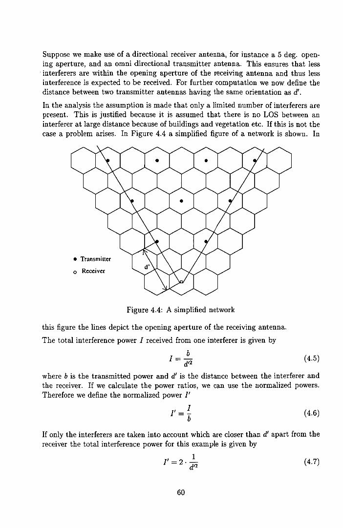
Suppose we make use of a directional receiver antenna, for instance a 5 deg. open­ing aperture, and an omni directional transmitter antenna. This ensures that lessinterferers are within the opening aperture of the receiving antenna and thus lessinterference is expected to be received. For further computation we now define thedistance between two transmitter antennas having the same orientation as d'.

In the analysis the assumption is made that only a limited number of interferers arepresent. This is justified because it is assumed that there is no LOS between aninterferer at large distance because of buildings and vegetation etc. If this is not thecase a problem arises. In Figure 4.4 a simplified figure of a network is shown. In

• Transmitter

o Receiver

Figure 4.4: A simplified network

this figure the lines depict the opening aperture of the receiving antenna.

The total interference power 1 received from one interferer is given by

b1 = d,2 (4.5)

where b is the transmitted power and d' is the distance between the interferer andthe receiver. If we calculate the power ratios, we can use the normalized powers.Therefore we define the normalized power l'

l' = ~b

(4.6)

If only the interferers are taken into account which are closer than d' apart from thereceiver the total interference power for this example is given by

1'=2.2- (4.7)d,2

60

If interferers from distance 0 to 2d' are taken into account this results in

, 1 1 ( )I = 2· d'2 + 3· (2d')2 4.8

Thus if interferers at an infinite distance from the receiver are taken into accountthe received interference power I' equals

and thus I' is given by

I' _ ~ i + 1- ~ (id')2

1 00 (1 1)I' = d,2 L "'7 + "72

i=I Z Z

(4.9)

(4.10)

Now one can see that the first term in the summation (I/i) does not converge. Thismeans that if there is a LOS with all interferers that the received interference powerwould become infinite. This is a problem for all cellular networks which are base ona LOS (high frequencies) and thus the received power is proportional to l/d2 .

In a practical situation there are always other attenuation mechanisms e.g. gaseousabsorption etc. These mechanisms further reduce the interference levels and helpto overcome the convergence problems. Furthermore it is assumed that there is noLOS from a specific receiver with all the transmitter antennas.

All the transmitters who are within the opening aperture and have a LOS withthe receiver produce interference. If the transmitter antennas are also of a direc­tional type, the interference can be further reduced because not every transmitterantenna within the opening aperture of the receiving antenna directs its maximumof electromagnetic energy towards the receiving antenna.

4.2.1 One direction line-up of the transmitter antennas

Assume that the cells are illuminated from the edge of the cello This can be accom­plished with a sectorial hom and still preserve the circularity of the cells [39]. Themost simple cellular structure with these antennas is to align all the transmitters asshown in Figure 4.5. FIOm this figure one can see that d = V3r and d' = V3d.

It is assumed that the transmitted signals are independent and thus the receivedpower interference may be added up. If we take three transmitters into account, t3

desired and tI and t2 interferers, the C/ I ratio CIR for worst case as in Figure 4.5is given by

C =10.10g ( b ;!1- b ) (4.11)I (a+d)2 + (a+2d)2

which results in

C I ( (V3r + a)2 . (2V3r + a)2 )I = 10· og a2. {(2V3r + a)2 + (V3r + a)2}

61

(4.12)

//

~ Transmitter

• Receiver

Figure 4.5: A simple aligned cell structure

where r is the radius of a eell and a is the distance between the receiver and thedesired transmitter t3.

Thus if the receiver is at the edge of the cell, a = V3r, the carrier to interference CII= 4.4 dB. Since this is not sufficient for most transmission systems, such a simpleSFN can never exist.

4.2.2 Rotated line-up of the transmitter antennas

The second approach to a single frequency network is to create acellular systemwhere the transmitter antennas which have the same orientation are as far apart aspossible [19]. The disadvantage of such a network is shown in Figure 4.6 where inregion A a receiver antenna is pointing directly to the transmitter of cell A but atan large angle a. The antenna gain in this particular direction is thus low. Thetransmitter antenna in cell B however is exactly pointing in the direction of thereceiver. The antenna gain of the interfering transmitter is thus at its maximum.This results in a high interference level because the received power is proportionalto lld2

•

In an alternative setup the goal is to make sure that the problem of the configurationabove does not occur. Now only three different orientations of the antennas are used.From this figure one can see that d = V3r and d' =3r.

The antennas with different orientations are positioned as far as possible apart, the

62

B

~ Transmitter

• Receiver

Cell

Figure 4.6: Incorrect configuration of cells

antennas with the same orientation are then much doser positioned to each other.

This results in the pattern shown in Figure 4.7.

The C/1 ratio then equals

for one interferer and

c _ 10 I ( (2~)2 )-- 'og--I (5~)2

(4.13)

(4.14)c = 10 . log ( 1 ~ 1 )I (5r)2 + (8r)2

if two interferers are taken into account.

The interference thus equals in the worst case 8 dB for one interferer and 6.5 dB fortwo interferers.

4.2.3 Rotated line-up using both polarizations

If the same configuration, as discussed in the previous section, is used but bothpolarizations are used, a "semi" SFN is constructed. This configuration shown inFigure 4.8. Again from this figure one can find the network parameters as, d = VJrand d' = 3r.

63

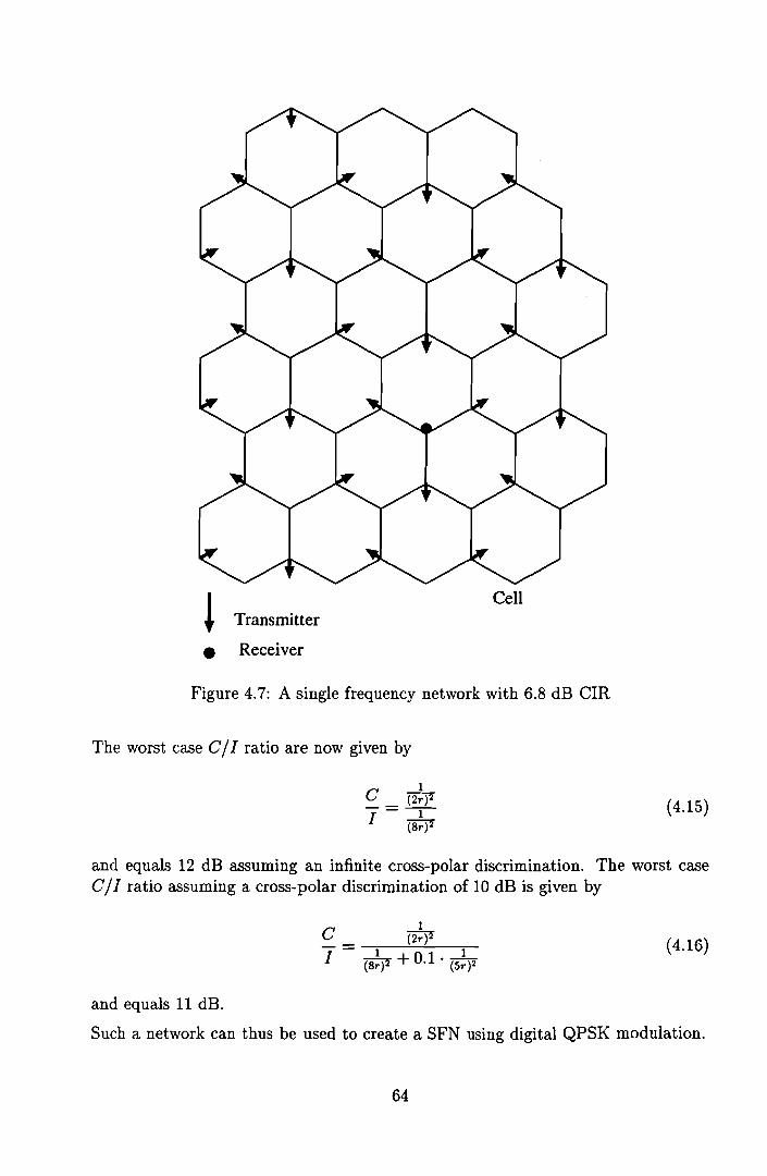
! Transmitter

• Receiver

eell

Figure 4.7: A single frequency network with 6.8 dB CIR

The worst case C/ I ratio are now given by

(4.15)

and equals 12 dB assuming an infinite cross-polar discrimination. The worst caseC/1 ratio assuming a cross-polar discrimination of 10 dB is given by

1C ~

I - (8~)2 + 0.1· (5;)2(4.16)

and equals 11 dB.

Sueh a network can thus be used to create a SFN using digital QPSK modulation.

64

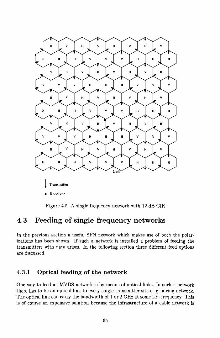
! Transmitter

• Receiver

Figure 4.8: A single frequency network with 12 dB CIR

4.3 Feeding of single frequency networks

In the previous section a useful SFN network which makes use of both the polar­izations has been shown. If such a network is installed a problem of feeding thetransmitters with data arises. In the following section three different feed optionsare discussed.

4.3.1 Optical feeding of the network

One way to feed an MVDS network is by means of opticallinks. In such a networkthere has to be an opticallink to every single transmitter site e. g. a ring network.The opticallink can carry the bandwidth of 1 or 2 GHz at some LF. frequency. Thisis of course an expensive solution because the infrastructure of a cable network is

65

expensive. The network could also use a coaxial cabie. This is approximately asexpensive as an opticallink but gives a smaller bandwidth.

A nice feature of such a network is that no outage time due to rain is introduced infeeding the network.

4.3.2 Feeding the network by satellite

Another solution is to feed the network by satellite. In this scenario at every trans­mitter site one or more satellite receivers are required. If the full eapaeity of anMVDS network is used more than one satellite has to be used to feed the network.In this scenario it is possible to have some different programs transmitted in differentceUs which ean be interesting.

4.3.3 Mutual feeding of the network

A third seheme is so-ealled mutual feeding by using every transmitter as a repeater.In a central cell of the network a digital signal is generated and transmitted to theadjacent cells. These eells retransmit the signaion their turn to their adjacent cellsetc.

To preserve the signal quality every cell has to demodulate the signal, perform theerror correction, recode the data and modulate it again. This is of course an option,if it is not used the result is error propagation through the network. The receptionantenna of a repeater/transmitter can be larger in dimensions, thus have a largerantenna gain and thus less outage time. Together with the error correcting eode itmay be possible to protect the signal for degradation. It is simple to introduce someredundancy by having every transmitter receive the same signal from two or morerepeaters. In this way it may be possible to further decrease the outage time.

In Figure 4.9 an example of the feeding of the network is shown.

In this figure three principle directions of feeding the network are shown. The arrowsrepresent the feeding directions.

From this picture one can easily see that every transmitter can be fed from two dif­ferent sources. The links between the transmitters are all shorter than the maximumpath length in a cell. If more redundancy is required it is possible for a transmittersite to receive from other transmitter sites at longer distances. If the antenna gainis increased by e.g. 6 dB approximately the double path length can be achieved.The line of sight requirement will probably be met beeause the transmitter antennasand thus also the reeeive antennas at the transmitter sites are mounted at a highposition.

Sinee the available bandwidth of a 42 GHz MVDS system is very large some localprograms can be inserted in one or more channels at a transmitter site.

66

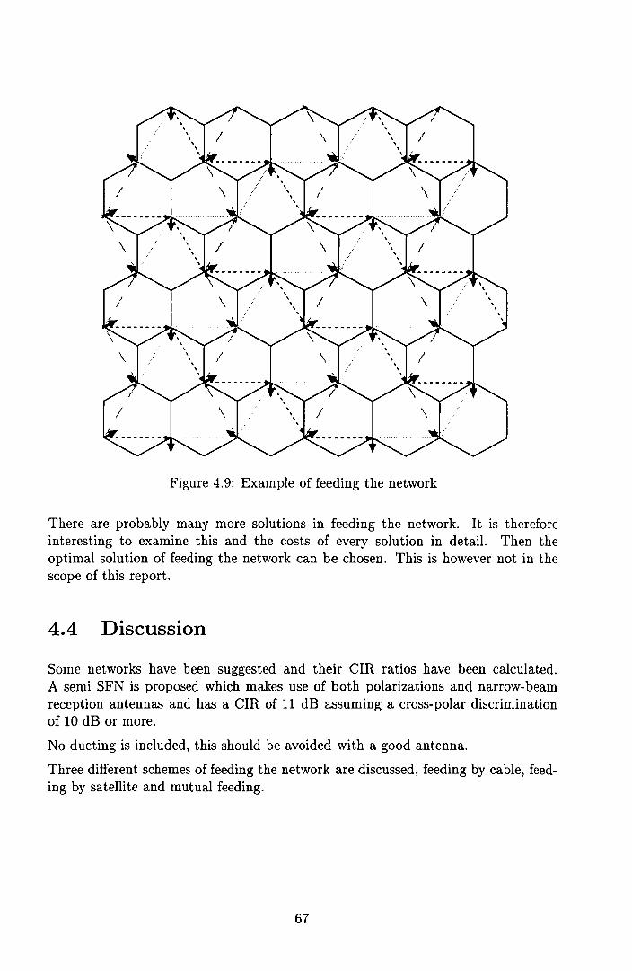
Figure 4.9: Example of feeding the network

There are probably many more solutions in feeding the network. It is thereforeinteresting to examine this and the eosts of every solution in detail. Then theoptimal solution of feeding the network ean be chosen. This is however not in thescope of this report.

4.4 Discussion

Some networks have been suggested and their CIR ratios have been ealeulated.A semi SFN is proposed which makes use of both polarizations and narrow-beamreception antennas and has a CIR of 11 dB assuming a eross-polar diseriminationof 10 dB or more.

No ducting is included, this should be avoided with a good antenna.

Three different schemes of feeding the network are discussed, feeding by cable, feed­ing by satellite and mutual feeding.

67

Chapter 5

Link budget calculations

Now we have discussed acellular structure in the previous section we are interestedin the celI sizes. Since the system aspects and the expected interference are knownit is in principle possible to calculate the link budget.

To calculate the link budget we must estimate the influence of noise and interferenceon the QPSK link.

5.1 Tolerabie noise and interference

To find the interference which can be tolerated the future system description briefiydiscussed in section 2.4 will be used. First the effect of noise on the digital link isdiscussed. Next the infiuence of interference and noise will be examined.

5.1.1 Influence of the Nyquist filter on the noise power

For the modulation scheme described in Section 2.4 the carrier to noise ratio C/ Nwhich is required for a quasi error free (QEF defined as a bit error rate BER of lessthan 10-11 ) link will be computed. To calculate the C/ N ratio in the transmissionchannel from the symbol energy Es to the noise power density No, often used indigital modulation, it is necessary to take the bandwidths of the different signalsinto account. In Figure 5.1 the different bandwidths are shown.

The required Es/No for a QEF QPSK operation using concatenated code are shownin table 5.1 [1].

The values Es/No are equal to the C/ N assuming QPSK. The values given howeverare the values before the demodulator as shown in Figure 5.2.

68

Signa! power

Bn=27.5 MHz);

Be=36 MHz (-3dB transponder bandwidth) .

kB~= 37.1 MHz

Figure 5.1: Definition of the theoretical bandwidths of a satellite channel

Inner code rate Es/No Gaussian channel (dB)1/2 3.12/3 4.93/4 5.95/6 6.97/8 7.7

Table 5.1: Required Es/No ratios (theoretical values)

The required channel bandwidth B~ can found with

(5.1)

where Ts is the symbol duration and Q is the roU-of! factor. The roU-of! factor usedin satellite transmission equals 0.35. As shown in Figure 5.1 however the adjacentbands do overlap. This results in e.g. a Nyquist bandwidth Bn of e.g. 27.5 MHzand a channel bandwidth Be of e.g. 36 MHz (B~ = 37.1 MHz). The symbol energyEs is defined as

fT.Es = Jo s(t)· s*(t) dt

69

(5.2)

36 MHz 27.5 MHz

~ IVNyqUist' I ~/ IDemodulatorl------7-)-

(~) Es ~Ne l'b N

Figure 5.2: The point of observation in the link

For QPSK this results in

(5.3)

(5.4)

where A is the amplitude of the carrier.

Assuming a white Gaussian noise with spectral density No. E 3 / No can written as

E 3 A2T3 Bn-=--.-No 2 N

where B n is the band width of the Nyquist filter and N = No' Bn is the noise powerafter the Nyquist filter.

The (C/ N)e is given by

( C) = A2

• Be (5.5)N c 2 N

where Be is the band width of the transponder and N = No' Be is the noise powerbefore the Nyquist filter.

The carrier power of the QPSK signal is given by

C = E 3 = A2

(5.6)T3 2

thus it is concluded that

Es = C = (1 + a') . (C)No N N e

where a' = 0.31 is the a corrected for the overlapping bandwidth.

, Bel+a =­

Bn

(5.7)

(5.8)

In table 5.2 the calculated values for the required Carrier to noise C/ N ratios as­suming a Gaussian channel are given for the different coding rates. These values donot include any system margin.

70

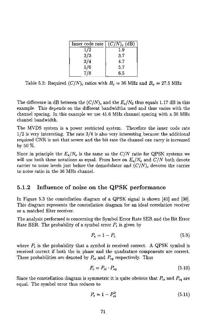
Inner code rate (C/N)c (dB)1/2 1.92/3 3.73/4 4.75/6 5.77/8 6.5

Table 5.2: Required (C/N)c ratios with Bc = 36 MHz and Bn = 27.5 MHz

The difference in dB between the (C/N)c and the Es/No thus equals 1.17 dB in thisexample. This depends on the different bandwidths used and thus varies with thechannel spacing. In this example we use 41.6 MHz channel spacing with a 36 MHzchannel bandwidth.

The MVDS system is a power restricted system. Therefore the inner code rate1/2 is very interesting. The rate 3/4 is also very interesting because the additionalrequired CNR is not that severe and the bit rate the channel can carry is increasedby 50 %.

Since in principle the Es/No is the same as the C / N ratio for QPSK systems wewill use both these notations as equal. From here on Es/No and C / N both denotecarrier to noise levels just before the demodulator and (C/ N)c denotes the carrierto noise ratio in the 36 MHz channe1.

5.1.2 Influence of noise on the QPSK performance

In Figure 5.3 the constellation diagram of a QPSK signal is shown [41] and [30].This diagram represents the constellation diagram for an ideal correlation receiveror a matched filter receiver.

The analysis performed is concerning the Symbol Error Rate SER and the Bit ErrorRate BER. The probability of a symbol error Pe is given by

(5.9)

where Pc is the probability that a symbol is received correct. A QPSK symbol isreceived correct if both the in phase and the quadrature components are correct.These probabilities are denoted by Pa and Pcq respectively. Thus

(5.10)

Since the constellation diagram is symmetrie it is quite obvious that Pci and Pcq areequal. The symbol error thus reduces to

(5.11)

71

•

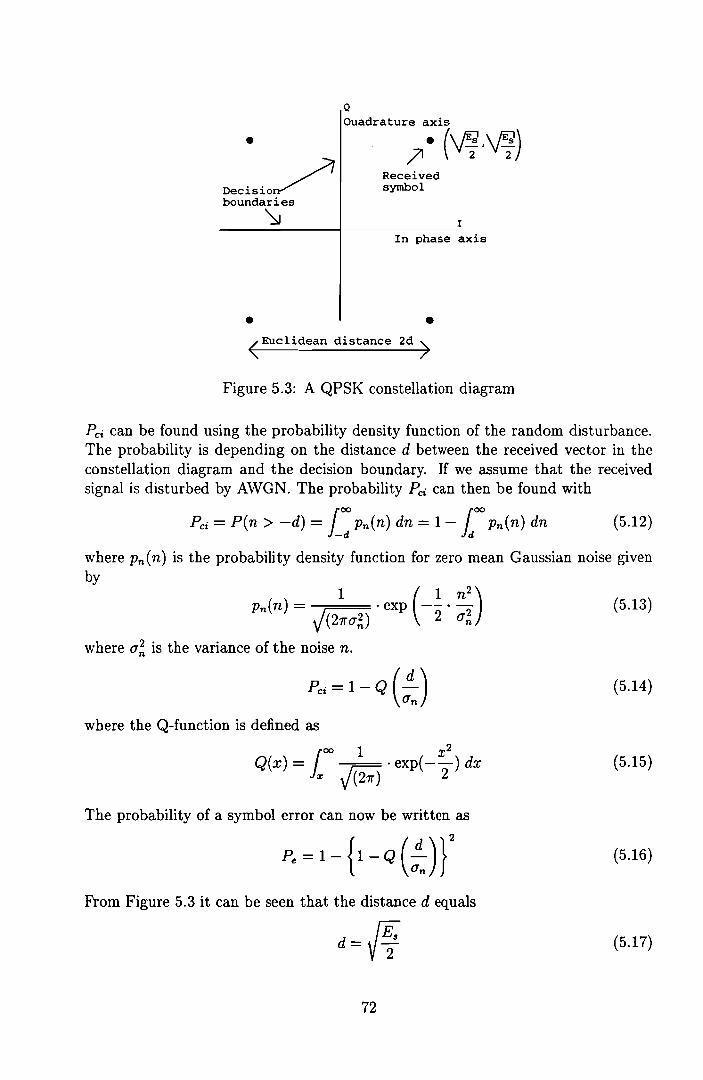
Decisio~boundaries

\J

•

Q

Ouadrature axis

~. (\f#.\f#)Receivedsyrnbol

I

In phase axis

•<Euclidean distance 2d >

Figure 5.3: A QPSK eonstellation diagram

Pci ean be found using the probability density funetion of the random disturbanee.The probability is depending on the distance d between the reeeived vector in theeonstellation diagram and the decision boundary. If we assume that the receivedsignal is disturbed by AWGN. The probability Pci ean then be found with

Pci = P(n > -d) = JOO Pn(n) dn = 1- [00 Pn(n) dn (5.12)-d Jd

where Pn(n) is the probability density function for zero mean Gaussian noise givenby

Pn(n) = 1 . exp (_!. n:)J(21ra~) 2 an

where a; is the varianee of the noise n.

PCi=l- Q (:n)where the Q-function is defined as

100 1 x2

Q(x) = r;;:;::\ . exp(--2) dxx V (21r)

The probability of a symbol error ean now be written as

From Figure 5.3 it ean be seen that the distance d equals

d=~

72

(5.13)

(5.14)

(5.15)

(5.16)

(5.17)

FIOm this the probability of a symbol error is found as

(5.18)

It is most likely that if an error occurs that the adjacent symbol is chosen. If the bitsare mapped on the symbols using the Gray-mapping one symbol error introducesonly one bit error and thus the BER or Pb equals

(5.19)

Assuming a small probability of error the total probability of a bit error is thusgiven by

(5.20)

With the formula above it is very simple to ealculate the bit error rate if the ratio(Es/No) is known. In Table 5.1 the required (C/N) ratio before the demodulator,or the (Es/No), is given. As an example we use the inner coding rate of 1/2 and wesee that (Es/No) of 3.1 dB is required. Using the formula above the eorrespondingprobability of error or BER ean be ealculated and equals 7 . 10-2 • It has beensimulated [1] that this BER ean be eorreeted to a QEF system or a bit rate of lessthan 10- 11 .

5.1.3 Influence of interference on the QPSK performance

The reeeived carrier may he impaired by other interferenee signals than the Addit­ive White Gaussian Noise (AWGN). Those interfering signals may come from theadjacent eells in acellular structure.

If we introduce an interferer our goal is to aehieve a BER of 7.10-2 so that the erroreorreeting seheme ean decrease the BER to 10-11

•

If it is assumed that the interfering signals and the desired signal are statistieallyindependent and in wide sense stationary random proeess of zero means [18] thereeeived power from the individual sourees may he added up.

The interferers will be the transmitters in the adjacent eells and thus also transmit­ting a QPSK signal. The mean of the signal is thus zero. Furthermore a QPSKsignal is a wide sense stationary proeess. Sinee the sources of the interfering signalsare at a relatively large distance it is even in an SFN reasonable to assume that thesignals are independent.

Thus the noise power plus interference power N equalsn

N=N+Ehk=l

73

(5.21)

where N is the total received noise power and h is the power of the kth interferer.

It is thus possible to calculate the maximum tolerabie interference if the noise powerand the carrier power are given. The calculations of the BER given Es/No are basedon a Gaussian noise source. To use these reslllts it is necessary that. t.he interferenceis also Gaussian distributed. If the number of individual interferers is large, havethe same distribution (none of them is dominant) and the individual distributionsare zero mean the joint probability density function of the interferers is Gaussiandistributed with a variance equal to the sum of the individual variances accordingto the central limit theorem.

If the received interference is dominated by one source and the probability densityfunction is not Gaussian the calculations based on the Gaussian assumption yielda pessimistic result [18]. This results on the given noise to interference ratio N/ I.In [18] it is stated that if the C/ I ratio is large (~ 20 dB) and at least 3 dB largerthan the C/ N ratio it is allowed to treat the interference as a Gaussian source (N/1~ 3 dB).

If the N / I ratio is small the system becomes interference dominated instead of noisedominated. In the future MVDS system the interference will be dominated by oneor very few interferers as is shown in the previous Chapter.

5.1.4 Worst case interference model

We will now derive a worst case model of the interference to estimate the impact ofthe interference.

If there is an interferer the constellation points in the constellation diagram aredisturbed in a random manner. This means that some disturbances actually improvethe tolerance to noise for that particular symbol as shown in Figure 5.4.

A worst case assumption is that the interferer is exactly synchronous with the re­ceived signal. This means that the sample time in the receiver samples at exact thecorrect time for the wanted signal as weIl as for the interferer. The output of thematched filter then produces the maximum output due to the interferer. Becausethe interferer is also a QPSK signal the filter is matched to the interferer as weIl.

If the modulation frequencies of the wanted signal and the interferer are exactlythe same it is allowed to model the interferer as a disturbance in the constellationdiagram. If the frequencies are not exactly the same the additional vector rotatesduring the signaling interval. It is worst case to have the interference vector in theworst case position throughout the whole signaling interval due to the integratingbehaviour of the matched filter. The BER can be written as a function of the angleof the interferer , with respect to the constellation diagram. This function can be

74

Transmitted Receivedsymbol symbol

•

necisio/boundaries

~

•

QInterference. ~ )

,?1 ,?1

I

•<Euclidean distance 2d >Figure 5.4: A constellation diagram with interferer

found using Formula 5.19 and is given by

Pb = ~ [1 - {1_Q (~ - ~ . COSh )) } . {1_Q (~ - ~ . Sinh )) }]

(5.22)where Ei is the energy of the interfering symbol and a "I of 0 corresponds to theinterferer given in Figure 5.4.

This function is plotted in Figure 5.5 for a C/ N ratio of 15 dB and a varying N/ Iratio. From this plot one can see that the worst case angle "I is 7T' or 3/21r. In theconstellation diagram this corresponds to the situation where the interferer pointstowards a decision boundary.

For our Worst case assumption we assume that the interfering signal is always at aworst case position, e.g. "I equals 7T', as shown in Figure 5.6.

All the above assumptions made thus far lead to a pessimistic upper bound for theBER. This analysis assumes however that the receivers carrier recovery and dockrecovery circuits work perfectly. For very low SNR or a high CIR this might notbe the case. This depends on the algorithms used and is beyond the scope of thisreport.

Another point is that the different carriers may run on nearly the same frequency.This results in slow rotating of the interferer in the constellation diagram. In thiscase the interference can be at a worst case position for a relative long time. Thiseffect can be interpreted as slow fading.

The probability of a bit error Pb can now be found using the formulae above (Figure

75

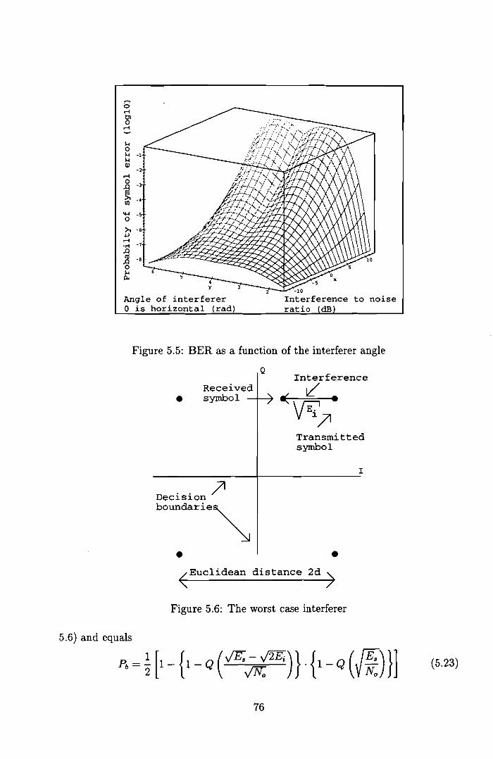
I-loI-l -1I-lal

.-loî -)lil

~ ­o>. -6oU.-l'M -7..Q11l

..QoI-lp..

Angle of interferero is horizontal (rad)

-10

Interference to noiseratio dB

Interference

-: IL'" •VE:7'

Receivedsymbol•

Figure 5.5: BER as a function of the interferer angle

Q

Transmittedsymbol

I

" 7'DeCloSloonboundarie~

• •<Euclidean distance 2d )

Figure 5.6: The worst case interferer

5.6) and equals

Pb = ~ [1- {1- Q (VE,~)}. {1- Q (~)}] (5.23)

76

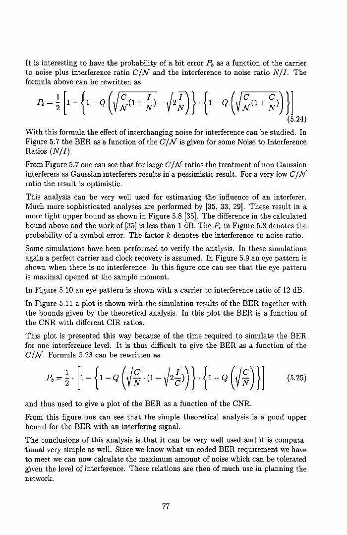
It is interesting to have the probability of a bit error Pb as a function of the carrierto noise plus interference ratio GIN and the interference to noise ratio NII. Theformula above can be rewritten as

Po=~ [1- {1- Q (J~{1+ ~)-ff)}. {l-Q (J~(l+ ~))}](5.24)

With this formula the effect of interchanging noise for interference can be studied. InFigure 5.7 the BER as a function ofthe GIN is given for some Noise to InterferenceRatios (NI1).

From Figure 5.7 one can see that for large GIN ratios the treatment of non Gaussianinterferers as Gaussian interferers results in a pessimistic result. For a very low GINratio the result is optimistic.

This analysis can be very weIl used for estimating the infiuence of an interferer.Much more sophisticated analyses are performed by [35, 33, 29]. These result in amore tight upper bound as shown in Figure 5.8 [35]. The difference in the calculatedbound above and the work of [35] is less than 1 dB. The Pe in Figure 5.8 denotes theprobability of a symbol error. The factor k denotes the interference to noise ratio.

Some simulations have been performed to verify the analysis. In these simulationsagain a perfect carrier and dock recovery is assumed. In Figure 5.9 an eye pattern isshown when there is na interference. In this figure one can see that the eye patternis maximal opened at the sample moment.

In Figure 5.10 an eye pattern is shown with a carrier to interference ratio of 12 dB.

In Figure 5.11 a plot is shown with the simulation results of the BER together withthe bounds given by the theoretical analysis. In this plot the BER is a function ofthe CNR with different CIR ratios.

This plot is presented this way because of the time required to simulate the BERfor one interference level. It is thus difficult to give the BER as a function of theGIN. Formula 5.23 can be rewritten as

(5.25)

and thus used to give a plot of the BER as a function of the CNR.

From this figure one can see that the simple theoretical analysis is a good upperbound for the BER with an interfering signal.

The condusions of this analysis is that it can be very weIl used and it is computa­tional very simple as weIl. Since we know what un coded BER requirement we haveto meet we can now calculate the maximum amount of noise which can be toleratedgiven the level of interference. These relations are then of much use in planning thenetwork.

77

0.01

0.001

y

0.0001

1e-OS

1e-OG

ie-07 0

L10 C 12

N+l

l/NdB

-100

Figure 5.7: The upper bound of the BER as a function of noise and interference

5.2 Link budget with noise

The link budget calculations are based on the provided service by the MVDS op­erator. We assume here that a service of a quasi error free performance is to beprovided for more than 99.9 % of the time. From this very low BER of 1 . 10-11

the BER before Viterbi decoding can be found if the coding rate is known. In thisreport two convolutional coding rates will be given as an example to calculate thelink budget; R = 1/2 and R = 3/4. From this un-coded BER the required Es/Nojust before the demodulator will be calculated. Further a implementation margin of

78

·CL

k - -13 ANO -21dBt---+-~--4\

k - -3 ---t--;--\-~\

k·. 2 ===::t:=:;l-4k-·'k-·'2--'"

10- 7 L....L......L..-L-...L....I.......1.....1....J.......L.....L....L.....!.......L.......L......L.....L.....L...I2 • & 8 la ,. 16

L

Figure 5.8: The upper bound of the BER as found by [35]

1 dB is taken into account. This value will then be converted to the required CNRin the channel. Prom this point on the transmission aspects as discussed in Section3 will be taken into account to calculate the maximum path length based on thesystem components characteristics and the maximum outage time. In this sectionthe results from the previous sections as wen as from the Appendices are used.

We will first calculate the link budget based on one cello Such a link budget is thusa noise limited budget since no interference is involved. In the following sectioninterference from adjacent ceUs is taken into account. This will change the linkbudget and thus the ceU sizes.

Prom Table 5.1 in Section 5.1 the required Es/No ratios are found for a QEF op­eration and equal 3.1 dB for a coding rate of 1/2 and 5.9 dB for a coding rate of3/4. Taking the effect of the root Nyquist filter into account we obtain the requiredG/N in the 36 MHz channel of 1.9 dB for R = 1/2 and 4.7 dB for R = 3/4. Now

79

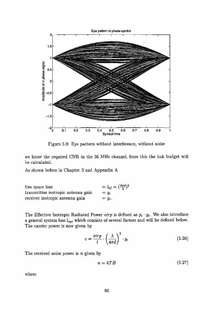
Eye pattem in phase symbol2.------...,--------,---,------.------.---r-----.-------,---.------,

1.5

aic:Cl

~ 0.51lI~CL

.ç; 0öCD"0

~-o.5CL

~-1

-1.5

0.90.80.3 0.4 0.5 0.6 0.7Symbol time

0.20.1-2 L-_....I...-_----I..__.L..-_...J...._--'-__-'--_...J...._--'-__...l..-_---l

o

Figure 5.9: Eye pattern without interference, without noise

we know the required CNR in the 36 MHz channel, from this the link budget willbe calculated.

As shown before in Chapter 3 and Appendix A

free space losstransmitter isotropic antenna gainreceiver isotropic antenna gain

- l - (41fd)2- bf- T= 9t= 9r'

The Effective Isotropic Radiated Power eirp is defined as Pt . 9t. We also introducea general system loss lsys which consists of several factors and will be defined below.The carrier power is now given by

c = eirp . (~) 2 • 9l 41rd r

(5.26)

The received noise power is n given by

n=kTB (5.27)

where

80

Eye pattem in phase symbol2.5r--....-----,---,--.,--......----,--,--....------,----,

2

(ijc::Cl'u;III 0.5~c-.5ë5al-g -0.5;t:

ëi

~ -1

-2

0.2 0.3 0.4 0.5 0.6 0.7 0.8 0.9Symbol time

0.1-2.5 '--_....1...-_---'-_----1.__-'---_--1.-_----'-__'--_....1...-_---'-_----'

o

Figure 5.10: Eye pattern with a CIR of 12 dB, without noise

k = Bo1tzmann's constant (JIK)T = the temperature (K)B = the receiving bandwidth (Hz).

This simp1e ana1ysis resu1t in the wen known formu1a [18]:

(5.28)

wherec = carrier powern = noise powereirp = Effective Isotropic Radiated Power1 = system 10ssd = distanceÀ = wave1engthk = Boltzmann constantB= receiving bandwidth9r = the receiver antenna gainT = the temperature.

81

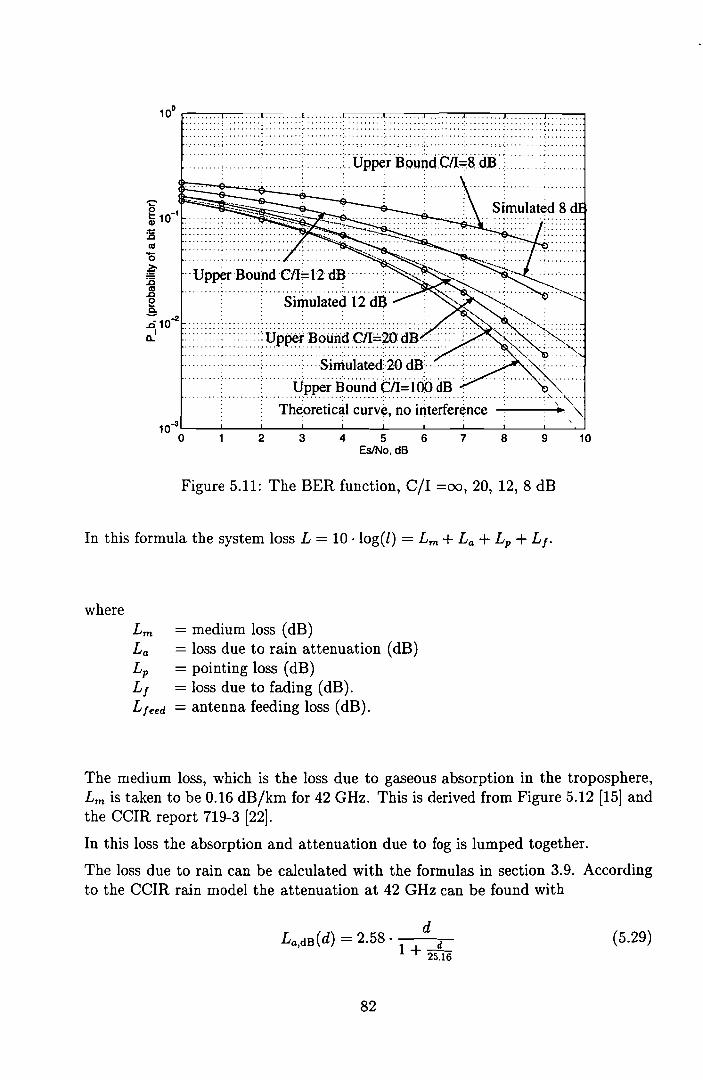
10° ,.--•.--,...c-:-.. ccc...-:T.C-:-•. c-:-.. ccc...--"..r.c-:-...ccc..--"..cr:--...ccc..--,... .,-,.. ccc...-..-.. -......-.. -...-.'.-.. -...-.."-'.-.. -...-..-......- ..-.. ---,..... ...... '.' : : ~ ; ..........: : : : : ... : : ... : ~;. ..: . : : : , ,: ~ .. . . . .. .;......:::.:.... ...... .. .......:Upper. t~öündtl.I~8.dB·~·······::::::::·:··

~~ 10-1

;t::.cal

Ö~

~~Co

:610-2.::::::::::::::::::::::::: .. ·· ...... · ... .

0.1 : ::: :::: >:::::::::ypp'# '~~~~~ç~~~: 4*..: :::::............... . .

.., . .. .. . .. Simulated 20 dB.. ... . . 'N" ... . lJp!Jëi-'l3öünt1 êii~ï ooëta . ' ~~ ......, ,.............................................. .. .... . ...'- "'.

. Theoretic~l curve, no interference '. '. '"

2 3 4 5 6EslNo, dB

7 8 9 10

Figure 5.11: The BER function, C/I =00, 20, 12, 8 dB

In this formula the system 10ss L = 10 ·log(l) = Lm+ La + Lp + Lf.

whereLm = medium 10ss (dB)La = 10ss due to rain attenuation (dB)Lp = pointing 10ss (dB)L f = 10ss due to fading (dB).L feed = antenna feeding 10ss (dB).

The medium 10ss, which is the 10ss due to gaseous absorption in the troposphere,Lm is taken to be 0.16 dB/km for 42 GHz. This is derived from Figure 5.12 [15] andthe CCIR report 719-3 [22].

In this los8 the absorption and attenuation due to fog is lumped together.

The 10ss due to rain can be calculated with the formulas in section 3.9. Accordingto the CCIR rain model the attenuation at 42 GHz can be found with

dLa,dB(d) = 2.58· d

1 + lli6

82

(5.29)

no21050 tOl5 tO

Froqucnq (GHz)

zez

H.O

)"

JOl -

J

,/

1/"-H.O VI \ J /\

" "r--..I I \

I \

/ / ~1/ / ""'-

t / ~Oau< 10GHI

0,'

'.005.,­to,

2

',05

0,02

10

I,.l t

~rJ ',2

I< o,t

Figure 5.12: Atmospheric attenuation by oxygen and water vapour[15]

for horizontal polarization and

dLa,dS(d) = 2.23· d

1 + 25.16

(5.30)

for vertical polarization, where d = path length in km between the transmitter andthe receiver.

The pointing 10ss originates from a fini te pointing accuracy. This can be aresuit frominstallation and wind effects on the antenna pole. It is supposed that the antennadefl.ection due to the wind shall not exceed 0.5 degree in any direction when subjectedto a 3 second wind gust of 45 mis as stated in the British Telecommunicationsspecifications 886003 [37],

The antenna gain pattern of a dish antenna can be approximated with a parabolic

83

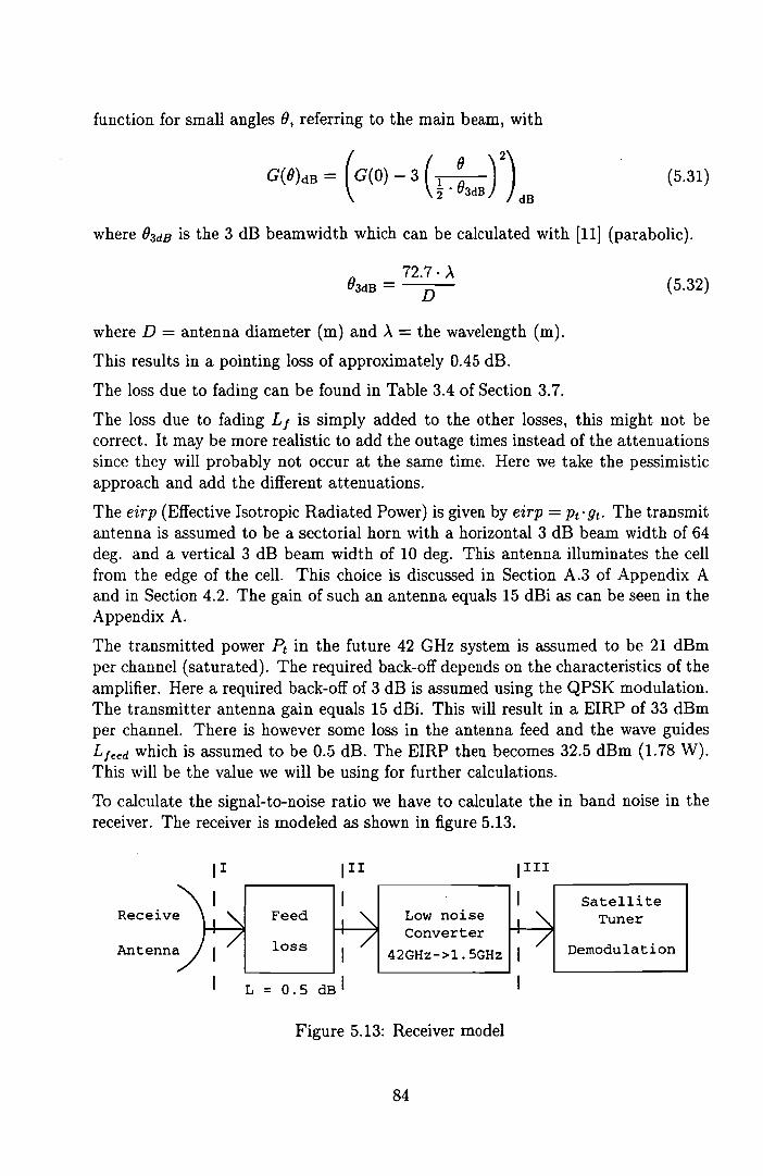
function for small ang1es (), referring to the main beam, with

G(O)dB = (G(O) - 3 (1.: )2)2 3dB dB

(5.31)

where ()3dB is the 3 dB beamwidth which can be calcu1ated with [11] (parabolic).

()_ 72.7·A

3dB - D(5.32)

where D = antenna diameter (m) and A = the wavelength (m).

This resu1ts in a pointing 10ss of approximate1y 0.45 dB.

The 10ss due to fading can be found in Tab1e 3.4 of Section 3.7.

The 10ss due to fading L / is simp1y added to the other losses, this might not becorrect. It may be more realistic to add the outage times instead of the attenuationssince they will probab1y not occur at the same time. Here we take the pessimisticapproach and add the different attenuations.

The eirp (Effective Isotropie Radiated Power) is given by eirp = Pt'gt. The transmitantenna is assumed to be a sectorial horn with a horizontal 3 dB beam width of 64deg. and a vertica1 3 dB beam width of 10 deg. This antenna illuminates the cellfrom the edge of the cello This choice is discussed in Section A.3 of Appendix Aand in Section 4.2. The gain of such an antenna equa1s 15 dBi as can be seen in theAppendix A.

The transmitted power Pt in the future 42 GHz system is assumed to be 21 dBmper channe1 (saturated). The required back-off depends on the characteristics of theamplifier. Here a required back-off of 3 dB is assumed using the QPSK modu1ation.The transmitter antenna gain equa1s 15 dBi. This will resu1t in a EIRP of 33 dBmper channel. There is however some 10ss in the antenna feed and the wave guidesL/eed which is assumed to be 0.5 dB. The EIRP then becomes 32.5 dBm (1.78 W).This will be the va1ue we will be using for further calcu1ations.

To calcu1ate the signa1-to-noise ratio we have to calcu1ate the in band noise in thereceiver. The receiver is modeled as shown in figure 5.13.

III IIll

SatelliteFeed Low noise Tuner

Converter1058

42GHz->1.5GHz Dernodu1ation

L = 0.5 dB I

Figure 5.13: Receiver model

84

It is assumed here that the down conversion is performed in 2 steps. In this conceptthe standard satellite down converter can be used and only the mixer (42 GHz to12 GHz) and the reception antenna has to be added. The noise figure of a satellitedown converter equals 1 dB. The first mixer has aconversion 10ss of 6 dB. For noisecalculations this mixer is modelled as a 10ss and thus it has a noise figure of 6 dB.Using Friis formula this results in a noise figure of 7 dB at reference plane IJ. It ispossible to add a 30 dB low noise MMIC amplifier just before the first mixer stage,the total noise figure at the antenna wave guide output can then be reduced to about5 dB. For further calculations the total noise figure of the receiver is taken 7 dB forthe production modeIs.

The effective temperature of the receiver at reference plane 11 thus equals 1163 K.The total system temperature equals

T sys = Tant,l I + Te (5.33)

where Tant,lI = the antenna noise temperature at the output of the wave guide andTe = the effective receiver noise temperature.

The antenna temperature at plane IJ can be calculated with

Tant,II = Tant,I . ga + (1 - ga) . Ta (5.34)

where ga is the available gain of the wave guide.

The 10ss of the wave guide L feed up to the converter is estimated at 0.5 dB. TA istaken 290 K as shown in Chapter 3. From this we conclude that for this system theantenna noise temperature Tant,II equals 290 K. The total system temperature atplane 11 thus equals 1453 K.

The gain of the receiver antenna (20 cm dish) equals 36 dB (efficiency from 0.5 to0.6). The figure of merit GIT then becomes 3.9 dB and is of course independentfrom the reference plane.

With the information summarized above the maximum path length is calculated andequals 5.74 km for vertical polarization and 5.33 km for the horizontal polarization.The cell radius determined by the horizontal polarization thus equals 2.87 km andits area equals 22.3 km2

•

In Table 5.3 the numerical results of the link budget are presented in tabular form.

5.3 Link budget with noise and interference

In the previous section the link budget was calculated. This resulted in a maximumcell diameter. Now we will introduce the interference as expected from Section 4and calculate again the cell diameter. One can see directly the influence of theinterference.

85

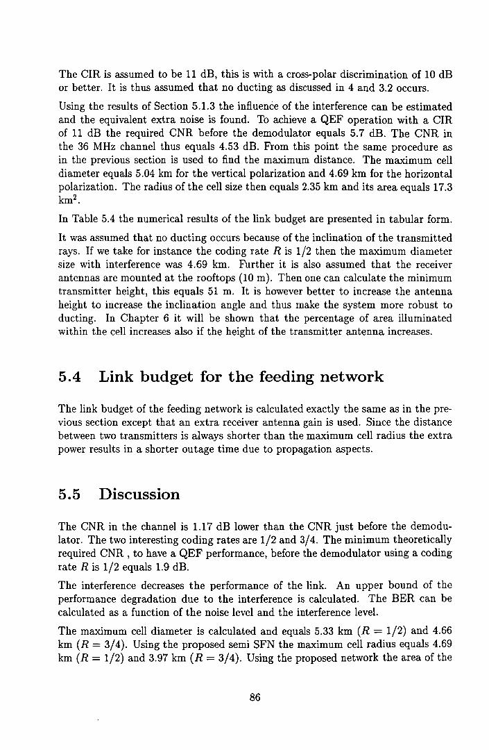
The CIR is assumed to be 11 dB, this is with a cross-polar discrimination of 10 dBor better. It is thus assumed that no ducting as discussed in 4 and 3.2 occurs.

Using the results of Section 5.1.3 the influence of the interference can be estimatedand the equivalent extra noise is found. To achieve a QEF operation with a CIRof 11 dB the required CNR before the demodulator equals 5.7 dB. The CNR inthe 36 MHz channel thus equals 4.53 dB. From this point the same procedure asin the previous section is used to find the maximum distance. The maximum celldiameter equals 5.04 km for the vertical polarization and 4.69 km for the horizontalpolarization. The radius of the cell size then equals 2.35 km and its area equals 17.3km2 •

In Table 5.4 the numerical results of the link budget are presented in tabular form.

It was assumed that no ducting occurs because of the inclination of the transmittedrays. If we take for instance the coding rate R is 1/2 then the maximum diametersize with interference was 4.69 km. Further it is also assumed that the receiverantennas are mounted at the rooftops (10 m). Then one can calculate the minimumtransmitter height, this equals 51 m. It is however better to increase the antennaheight to increase the inclination angle and thus make the system more robust toducting. In Chapter 6 it will be shown that the percentage of area illuminatedwithin the cell increases also if the height of the transmitter antenna increases.

5.4 Link budget for the feeding network

The link budget of the feeding network is calculated exactly the same as in the pre­vious section except that an extra receiver antenna gain is used. Since the distancebetween two transmitters is always shorter than the maximum cell radius the extrapower results in a shorter outage time due to propagation aspects.

5.5 Discussion

The CNR in the channel is 1.17 dB lower than the CNR just before the demodu­lator. The two interesting coding rates are 1/2 and 3/4. The minimum theoreticallyrequired CNR , to have a QEF performance, before the demodulator using a codingrate Ris 1/2 equals 1.9 dB.

The interference decreases the performance of the link. An upper bound of theperformance degradation due to the interference is calculated. The BER can becalculated as a function of the noise level and the interference level.

The maximum cell diameter is calculated and equals 5.33 km (R = 1/2) and 4.66km (R = 3/4). Using the proposed semi SFN the maximum cen radius equals 4.69km (R = 1/2) and 3.97 km (R = 3/4). Using the proposed network the area of the

86

cells then becomes 17.3 km2 (R = 1/2) and 12.3 km2 (R = 3/4). The minimumtransmitter height equals 51 m (R = 1/2) and 44.6 m (R = 3/4).

Using the narrow-beam reception antennas the pointing loss is not negligible. Thesystem noise temperature Tsys equals 1453 K, the figure of merit (G/T) equals 3.9dB.

The outage time chosen here equals 0.1 % and is based on the outage time in directbroadcasting satellites. In broadcasting it is very common to have an outage timeof 0.01 % or 0.03 % of the time. It is believed that for a commercial usage of anMVDS system 0.1 % outage time is acceptable.

The outage time influences the link budget dramatically of course. The link budgetcalculated however is just an indication and an example. Many more parameters inthe link can be varied which decrease or increase the area covered.

87

Rate R = 1/2 Rate R = 3/4Requirements

1 Coded HER - 1. 10 -11 1 . 10 ·u2 Un-coded BER 7.4.10-2 2.4 .10-2

3 Link availability 99.9 % 99.9 %4 Imp1ementation margin (M) 1 dB 1 dB

Required CNR ratios5 CNR before demodulator 3.1 dB 5.9 dB6 CNR in channe1 1.9 dB 4.7 dB

Transmitter7 Saturated power (Ps) -9dBW -9dBW8 Output back-of! (BO) 3 dB 3 dB9 Radiated power (Pt ) -12 dBW -12 dBW10 Transmit antenna gain (G t ) 15 dBi 15 dBi11 Transmit feed 10ss (L feed ) 0.5 dB 0.5 dB12 EIRP = Ps - BO + Gt - Lfeed 2.5 dBW 2.5 dBW

Channel13 Free space 10ss (Lbf ) 139.4 dB 138.3 dB14 Medium 10ss (Lm) 0.852 dB 0.746 dB15 Rain attenuation (La) 11.34 dB 10.14 dB16 Mu1tipath fade margin (L f ) 3.90 dB 3.59 dB17 System 10ss Lsys = Lbf + Lm+ La + Lf 155.5 dB 152.7 dB

Receiver18 Receive antenna gain (Gr) 36 dBi 36 dBi19 Pointing loss (Lp) 0.45 dB 0.45 dB20 Receiver feed 10ss (L feed ) 0.5 dB 0.5 dB21 Tota1 receiver gain G = Gr - Lp - Lfeed 35.05 dB 35.05 dB

Noise22 Receiver noise figure (F) 7 dB 7 dB23 Receiver noise temperature (Tr) 1175 K 1175 K24 Antenna noise temperature (Ta) 290 K 290 K25 System noise temperature Ts = Ta + Tr 1465 K 1465 K26 Channe1 noise Bandwidth (B) 75.6 dB Hz 75.6 dB Hz27 Noise due to interference (Ni) odB odB28 Boltzmann's constant (k' = 1010g(k)) -228.6 dBW/K/Hz -228.6 dBW/K/Hz29 Noise Power N = k' + 10 10g(Ts) + B + Ni -121.3 dBW -121.3 dBW

Receive levels30 Faded iso. rec. level = EIRP - M - Lsys -154 dBW -151.2 dBW31 Faded rec. level = EIRP - M - L•..• + G -119 dBW -116.2 dBW

~::I~ -

Coverage32 Path 1ength 5.33 km 4.66 km33 coverage area 22.3 km2 17 km2

Tab1e 5.3: Link budget with noise (no interference)

88

Rate R = 1/2 Rate R = 3/4Requirements

1 Coded BER 1. 10 ·11 1.10 ·11

2 Un-coded BER 7.4.10-2 2.4. 10-2

3 Link availability 99.9 % 99.9 %4 Implementation margin (M) 1 dB 1 dB

Required CNR ratios5 CNR before demodulator 3.1 dB 5.9 dB6 CNR in channel 1.9 dB 4.7 dB

Transmitter7 Saturated power (Ps) -9 dBW -9dBW8 Output back-off (BO) 3 dB 3 dB9 Radiated power (Pt ) -12 dBW -12 dBW10 Transmit antenna gain (Gt ) 15 dBi 15 dBi11 Transmit feed loss (Lleed) 0.5 dB 0.5 dB12 EIRP = Ps - BO + Gt - Lfeed 2.5 dBW 2.5 dBW

Channel13 Free space loss (Lbl ) 138.3 dB 136.9 dB14 Medium loss (Lm) 0.75 dB 0.635 dB15 Rain attenuation (La) 10.19 dB 8.85 dB16 Multipath fade margin (L f ) 3.60 dB 3.26 dB17 System loss Lsys = Lbf + Lm+ La + LI 152.9 dB 149.6 dB

Receiver18 Receive antenna gain (Gr) 36 dBi 36 dBi19 Pointing loss (Lp) 0.45 dB 0.45 dB20 Receiver feed loss (L feed ) 0.5 dB 0.5 dB21 Total receiver gain G = G r - Lp - Lfeed 35.05 dB 35.05 dB

Noise22 Receiver noise figure (F) 7 dB 7 dB23 Receiver noise temperature (Tr) 1175 K 1175 K24 Antenna noise temperature (Ta) 290 K 290 K25 System noise temperature Ts = Ta + Tr 1465 K 1465 K26 Channel noise Bandwidth (B) 75.6 dB Hz 75.6 dB Hz27 Noise due to interference (Ni) 2.63 dB 3.13 dB28 Boltzmann's constant (kt = 10 log(k)) -228.6 dBW/K/Hz -228.6 dBW/K/Hz29 Noise Power N = kt + 10 10g(Ts) + B + Ni -118.7 dBW -118.2 dBW

Receive levels30 Faded iso. rec. level = EIRP - M - Lsys -151.4 dBW -148.1 dBW31 Faded rec. level = EIRP - M - Lsys + G -116.3 dBW -113.1 dBW

Coverage32 Path length 4.69 km 3.97 km33 coverage area 17.3 km2 12.3 km2

Table 5.4: Link budget with noise and interference

89

Chapter 6

Expected coverage in a city

Now it is possible to calculate the cell size from the previous Chapter, one is veryinterested in the coverage within a cell (the number of homes seen). In Section 3.4it is shown that diffraction at high frequencies is not very useful. The diffractionloss increases very rapidly if the diffraction angle increases. This means that forreception of MVDS signals there has to be a direct LOS between the transmitterand the receiver or a "semi" LOS, i.e. a LOS if one reflection on a good reflectingsurface is allowed. Since one reflection attenuates the signal approximately 10 dB, itis only in a small part of the coverage area possible to make use of a reflection. Themaximum path length with one reflection can be calculated with the link-budget inChapter 5 if one takes into account an extra loss of 10 dB.

The total coverage area served for 99.9% of the time is 17.3 km2 (maximum range is4.69 km). If an extra attenuation of 10 dB is included (one reflection) the maximumpath length reduces to 2.7 km. The reception sites who can actually make use of areflection must have a maximum path length (reflection) of 2.7 km and furthermorethere must be a good reflecting surface at the correct position and at the correctangle. This further reduces the possibilities of reception by means of a reflection. Itis thus concluded that the increase in the percentage of coverage due to a reflectionwill be very small if not negligible.

Ir an MVDS operator wishes to exploit an MVDS system in a given area he wishesto predict the number of homes seen in that area. This is very interesting if notessential for MVDS operators. Using such an estimation the value of a future MVDSnetwork can be calculated on fore-hand.

To estimate the percentage of coverage in a cell or the number of homes seen, aprogram has been written which predicts the possibilities of reception within a givencity. The input of this program is either a deterministic presentation of the city(coordinates of buildings, heights, rotation angles, sizes) or a statistical distributionof the sizes and heights of the buildings within a city. If the statistical approach isused the program generates random but typical cities and calculates the percentageof coverage within the generated cities.

90

The program is in principle a 3-D ray tracing program. It tries to find from everyloeation within the eeU either a LOS or a semi LOS to the transmitter antenna. Theextra percentage in coverage due to reflections ean thus be very weIl studied withthis program.

With this program it is also possible to calculate the most interesting antenna heightand position of the transmit antenna, the eosts of the antenna mast constructioncan then be compared with the value of the future MVDS network with that specificantenna height.

In Figure 6.1 the graphical presentation of part of the city of Eindhoven is shown.The circle depicts the eeIl with a radius of 2.5 km and the squares are the highbuildings within this part of Eindhoven.

Figure 6.1: The graphical presentation of Eindhoven

The different colors of the buildings denote the height of the buildings. The transmitantenna at the NatLab building WY with a height of 65 m is positioned at theleftmost position of the ceIl (smaIl circle).

We will now predict the coverage within the city of Eindhoven as an example. Firstwe will only use the LOS and secondly also refiections will be included.

91

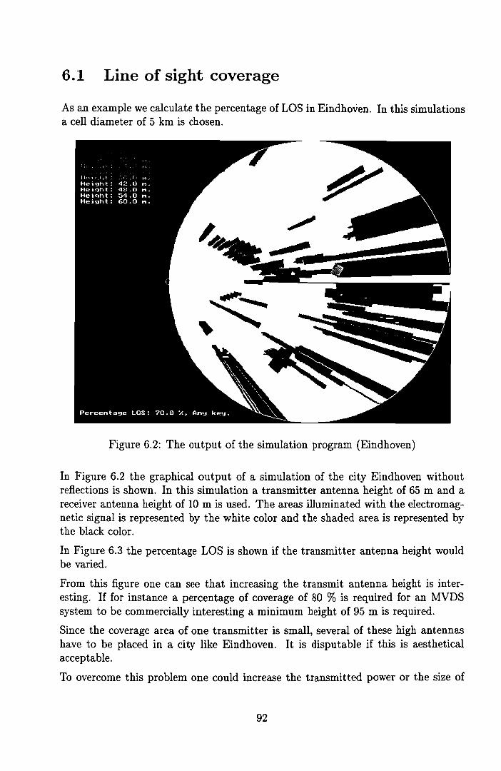
6.1 Line of sight coverage

As an example we calculate the percentage of LOS in Eindhoven. In this simulationsa cell diameter of 5 km is chosen.

Figure 6.2: The output of the simulation program (Eindhoven)

In Figure 6.2 the graphical output of a simulation of the city Eindhoven withoutreflections is shown. In this simulation a transmitter antenna height of 65 mand areceiver antenna height of 10 mis used. The areas illuminated with the electromag­netic signal is represented by the white color and the shaded area is represented bythe black color.

In Figure 6.3 the percentage LOS is shown if the transmitter antenna height wouldbe varied.

From this figure one can see that increasing the transmit antenna height is inter­esting. If for instance a percentage of coverage of 80 % is required for an MVDSsystem to be commercially interesting a minimum height of 95 m is required.

Since the coverage area of one transmitter is small, several of these high antennashave to be placed in a city like Eindhoven. It is disputable if this is aestheticalacceptable.

To overcome this problem one could increase the transmitted power or the size of

92

I-.. "

......

i.·······.................

.........................

..... "" ......

: ,

100

80

~Cl>

~ 60

BëCl>Cl111c 40~Cl>lL

20

o20 40 60 80 100

Transmitter anlenna heighl h_l[m)120 140

Figure 6.3: LOS as a function of the transmitter antenna height

the receiver antennas and thus increase the area covered. This reduces the numberof high positioned transmit antennas in a given area. An other option is to raisethe reception antennas (currently 10 m) such that the transmitter antenna can belowered to achieve the same percentage of coverage. In Figure 6.4 the increase incoverage due to increasing the receiver antenna height is shown with a transmitterantenna height of 65 m. Both options are again aesthetical not desirabIe. A tradeoffof the problems mentioned above has to be made. The outcome depends very muchon the environment and can be predicted with this program.

In Figure 6.5 an example is shown of a statistical approach of the simulations. Inthis simulation the transmitter height was 65 mand the receiver height was 10 m.The width and length of the buildings was uniformly distributed from 10 to 60 m,the height of the buildings was uniformly distributed from 20 to 65 mand a totalof 90 buildings were generated. The cell diameter again equals 5 km. A numberof runs have been performed and the result was an average cell coverage of 71.6 %.This statistical model is thus a usabIe model for the city of Eindhoven.

6.2 Coverage using refiections

Now refiections are included in the prediction program, such that the increase in thepercentage of coverage can be found. In Figure 6.6 the graphical output with perfectrefiections is shown. This means that the extra path length and the refiection lossis not taken into account.

The gray color in this diagram represents the area covered by means of a refiection.

93

85

80

I8o 75

fl

70

.•.•.....•..•..•..•..

.................•.....

....•••...•••..•.•...•..... ,.'

l....·····················...•......•........•......

6510 12 14 16

Receiver antenna height h_t [mI18 20

Figure 6.4: The coverage with increasing receiver antenna height

In Figure 6.7 the percentage LOS and semi LOS is shown again as a function of thetransmitter antenna height. In this figure the LOS without refiections and usingone refiection is shown. This is however assuming a perfect refl.ection. One can seethat the increase in percentage of coverage, even with perfect refl.ections, in the cityof Eindhoven is very small.

If the refiection loss is taken into account the maximum path length with one re­f1.ection becomes 2.92 km. The coverage gain due to refl.ections is then even smaller.This is because the relative large distance between the transmitter and the highbuildings in the center of the city. In Figure 6.8 the graphical simulation result isshown and in Figure 6.9 the numerical simulation result is shown.

From this simulation it is concluded that planning service coverage relying on re­f1.ections makes no sense in the city of Eindhoven.

6.3 Discussion

It has been shown that the coverage within a city ean be predicted. The difficultpart is however to obtain the data of the buildings in the city. If these data areavailable, or alternatively the distributions of the dimensions of the buildings, it ispossible to predict the coverage in a city.

The increase in coverage in a cell due to accepting one refiection can be very wellstudied with this program and it is concluded that it is negligible in an environmentas the city of Eindhoven.

94

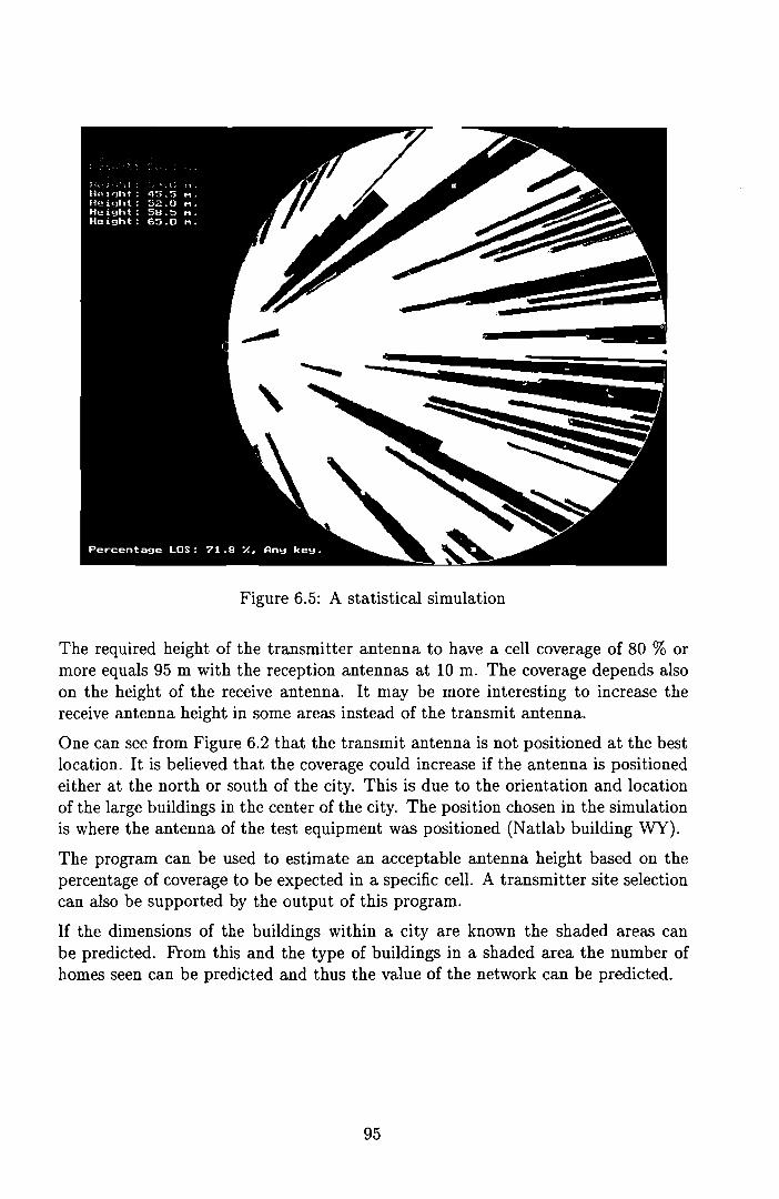
Figure 6.5: A statistical simulation

The required height of the transmitter antenna to have a cell coverage of 80 % ormore equals 95 m with the reception antennas at 10 m. The coverage depends alsoon the height of the receive antenna. It may be more interesting to increase thereceive antenna height in some areas instead of the transmit antenna.

One can see from Figure 6.2 that the transmit antenna is not positioned at the bestlocation. It is believed that the coverage could increase if the antenna is positionedeither at the north or south of the city. This is due to the orientation and locationof the large buildings in the center of the city. The position chosen in the simulationis where the antenna of the test equipment was positioned (Natlab building WY).

The program can be used to estimate an acceptable antenna height based on thepercentage of coverage to be expected in a specific cello A transmitter site selectioncan also be supported by the output of this program.

Ir the dimensions of the buildings within a city are known the shaded areas canbe predicted. From this and the type of buildings in a shaded area the number ofhomes seen can be predicted and thus the value of the network can be predicted.

95

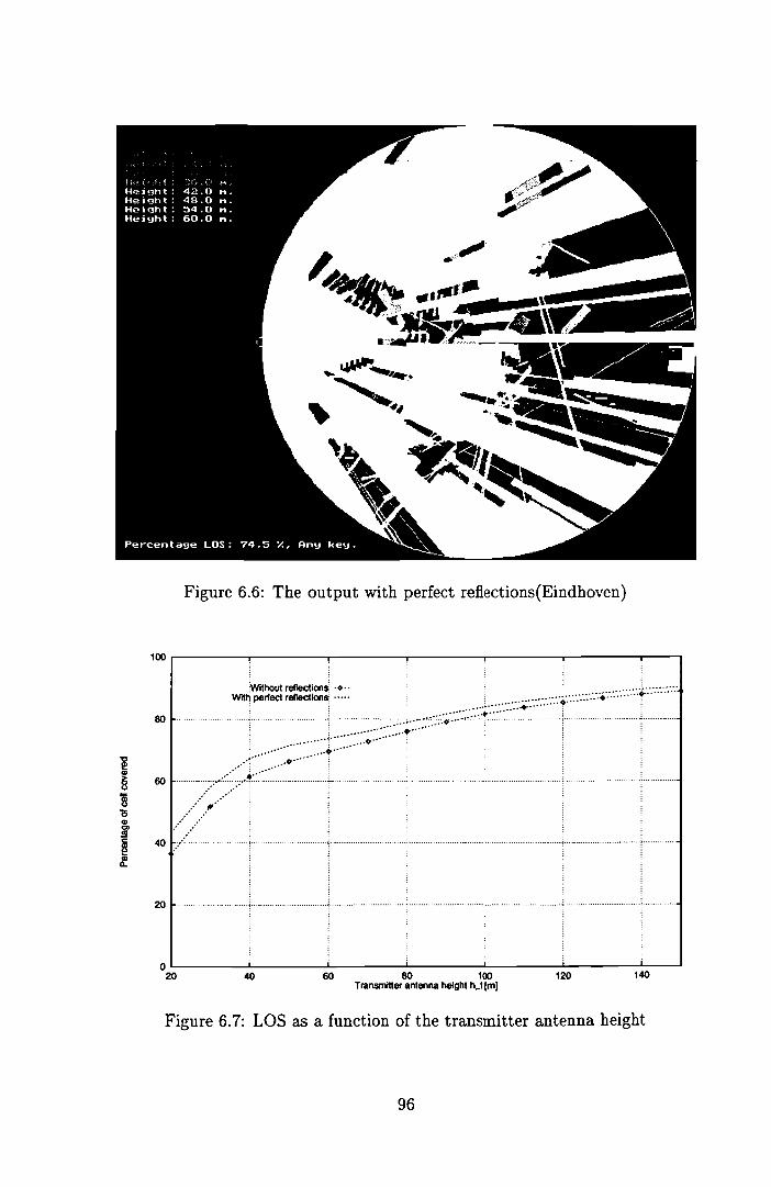
Figure 6.6: The output with perfect reflections(Eindhoven)

100 r----...-------.----___,----~---__r_---___r-___,

.....................!

.................................! .

,

. ..• .•.•.•• 't ~ .20

j ~ ..~Wrthout reflection~ .0··· ::

wrtri perfect reflection$ .....

80 _ .

60

40 ::::::: ~........ +... ;

14012060 80 100Transmitter antenna helght h_t [mI

40

OL- ...l...- ......L. ---l'-- ..i..- ....i.- --'-_----l

20

Figure 6.7: LOS as a function of the transmitter antenna height

96

Figure 6.8: The coverage with refiections in Eindhoven

14012060 80 100Transmitter antenna helght h_t (mI

40

....... ... .......

l,:,:,,:":~';;'"''''''.,..,~."..~.:.".~." •....•..

Wrth reftectilllll ......."",

........:::." .."" ...•...:::::::::ó·::::··

...:...::::::::::':, ~:::::;;-

.:/:/

./::....... ,:/,.•

.:::::::'

90

4020

50

70

55

75

80

85

60

65

45

Figure 6.9: LOS with refiection as a function of the antenna height

97

Chapter 7

Measurements

In this Chapter, measurements are described which were performed in January 1995.The measurements were performed with the 28 GHz link as described in AppendixA. The measurements are very time consuming, therefore only a limited number of63 measurements were performed at 37 locations. The object of the measurementstherefore is to observe some phenomena rather than produce a model. The pro­duced data are however still very interesting to confirm the theoretical models. Themeasurements also yield insight to the propagation aspects.

In Figure 7.1 a diagram of the measurement setup is shown.

This block diagram shows the transmitter setup as wen as the receiver setup. Alongthe blocks the expected power level at that point in the link is given. The factor Lin this diagram represent all the losses in the propagation path. The specific lossescan be found in the Appendix A or report [39].

The measurements were performed to get an impression of the propagation aspectsat 28GHz. The aspects of interest were:

• the possibilities of a LOS within a city.

• the attenuation if the LOS is obstructed.

• loss due to foliage.

• refiection of buildings within the city.

• refiection coefficients of building materia1s.

• robustness with respect to unwanted refiections.

• usefulness of diffraction around obstacles.

• depolarization of the electromagnetic waves.

98

PAL

Signal souree

(21 dllm) 120.5 dBm) (35.5 dBm)

No souree

wunodulate<!carrier

Triangular

sillrlal

30 IcHz

(35.5 - L dllm)

Pre-emphasis~---iI

Power Bupply

Indoor tr4llsmîtunit

Preamp. off ifnon PAL souree isselecte<!

(66 - L dBm) (100 - L dBm)

FM lIlOdulator

Gunn Oscillator

OUtdoor transmit Transmitter antennaunit

Mixer

amplifier

OUtdoor receiveunit

(87.4 - L dBm)

cable10s9

2 d8

cable

10ss

10.6 dB

Power

Supply

Spectrum

Analyser

SatelliteTuner

OemodulationDe-emphasis

Indoor receiveunit

Data

acquisition

ccnnputer

PAL

Display SOuree

Plotter

(85.4 - L dBm)

Figure 7.1: The measurement setup

In Figure 7.2 the results of the field trial are shown. The continuous line representsthe expected power if the only propagation loss is the free space loss Lbf • The +marks represent the measured values if the link was a LOS link. The rectanglesrepresent values measured with a known obstruction. At three places there was noreception possible these measurements are denoted with the crosses.

7.1 Link budget verification

The measurements matched the calculated link budget in report [39] very weIl.Therefore it is concluded that the power decreases simply according 1/r2• In Ap­pendix Bit was shown that indeed that it is expected that the power should decreasewith 1/r2 instead of the 1/r4 often used in urban areas.

During these measurements it is shown that, as expected, a LOS is required betweenthe transmitter and the receiver. Some obstruction can be tolerated e.g. a small

99

-30 r;:-----.---,------,r-----.---T""----,---""T"""---,...,

-40

ECD~(ij> -50

+~"'C lIlI~ 0:JUI«lQ)

E -60(ij B> 0~c:0

a -70 00Q)

u0~ 0

"'C 0Q)

üQ) -80Q.)(

W

+ LOS-90 0 Obstruction x x x

x No reception possible

500 1000 1500 2000 2500 3000 3500 4000 4500Distance [m]

Figure 7.2: Measurement results

tree. The power decreases however very rapidly if the first Fresnel zone is not freeof obstruction all over the radio path. For instance it has been found that a singletree can attenuate the received power in the order of 20 to 30 dB.

The measurements have also shown that the height of the receiver antenna shouldhe at the rooftops of the houses. If the antenna height is reduced the percentage ofsites which can receive the signal rapidly decreases.

No ducting was found, this is there were no measurements of receiving significantlymore power than expected using the calculations of free space loss Lbf •

7.2 Reflection

The possibility of reception via a refiection has been confirmed. The measurementsshowed that refiection coefficients as calculated in Section 3.5 can be used.

The absolute values of the orthogonal refiection coefficients measured in a practicalsituation at 28 GHz are in the order of 0.2 for brick at an angle of 10 deg. and 0.3for concrete at an angle of 20 deg. If we compare this with the Fresnel refiectioncoefficients it is concluded that the variance (J in the model of Beckmann would be

100

1.1 mm for brick and 0.92 mm for concrete. The actual values were not available.

It is concluded from measurements that in a practical environmental situation thelosses from one refiection are in the order of 10 dB or more for concrete or brick.

From this information it is easy to predict at what distance effective use can be madeof the a refiection under a specified angle. Within a coverage area it is possible todraw lines to which it is possible to make use of refiections. Whether the refiectionscan be of any use will highly depend on the layout of the coverage area. In theNetherlands for instanee there are very few high buildings in comparison to ordinaryhouses in a city. In sueh a case it is believed that the extra percentages of coveragedue to effectively making use of a refiection is very low. If in an other situationthe city is build up of almost all tall buildings the reception by means of refiectionmight be the only way to have some coverage in such an area. In Chapter 6 this issimulated.

Echoes can be a severe problem in a digitallink. The impulse response is thereforevery important. It is obvious that the impulse response is very dependent on theenvironment, type of buildings etc.

In the measurements done in January some refiections have been found. In Figure7.3 a received spectrum is shown which suffers severely from frequency selectivitydue to refiections. The distance between the notches in the frequency response !:::J.f

REF -10.0 dBm ATT 00 dB r-IKR 1442. 27 r-IHz

I I I- OOT - r r" I --

: --t- --~l" --t '--- -[ I---~..--- i-r--- r--- --. T .(.- (---: -- -- ....·---r----iT---i---- --t--r---î-- -'1--'---

-----,----.~4;od- m

I i: i ,_....- -I.--.+._...~·:-- -- ... --.,- ....

I ; i i !···-··--i--···-·;· ·----·'r- ._......i --- _.•_--~--•• ~ --- --~ .--...:.----

I I I ~ I;

-~.-···-·i---~.-.-- ---..- -"---!"---'---~'-----I-----'~----"---··j-·--..··t- --1·----- - ._-+ .. ···+··-1----···- T' .... I I I .! ! i . !

10 dB/

1 MHz

RBW

300 kHz

pas PK

VBW

SWP 50 m.. SPAN 30 MHz CENTER 1442.2 MHz

Figure 7.3: The received spectrum with multipath reception

equals 4.8 MHz. The time difference !:::J.t between the two received signals thus equals208 ns and the path length difference !:::J.s equals 62.5 m. With the signalling rate of27.5 M symbols per second this means the delay equals 5.7 symbols. From Figure7.3 one can also estimate the CIR, this is approximately 6.4 dB. In Chapter 4 we

101

have seen that this level of interference is unacceptahle. Since the two signals arecorrelated this could he solved with an equalizer however.

Figure 7.3 was found after mispointing the receive antenna on purpose. It has alsoheen shown however that at every location measured the received spectrum wascompletely free of frequency selectivity if the antenna was correctly positioned. InFigure 7.4 the spectrum is shown measured at the same location as in Figure 7.3 hutwith the antenna aligned correctly. It is therefore concluded that in an environment

1442.53 MHz

-52;3 d8m

.. i

ii

!

i " V\ 1

1

I i .! ~

MI<R

"-'. _.__.- -- .....~_.I

.. _-'----f---

'- -1------.. -

ATT 00 dB

I· ·-1! I

...._-- ._..... 1\""-' _.- _. - - _..

10 dB,'

REF -10.0 dBm

: \ !

: .t...Lt..1..IlI .,' ."

--- -- ....~.. -~~ ~.~ --=-._-+--f--_"-~_---I- ..--.1 .. ..

'----------'----'------'---.1...----..1...-------'------~_.L_SWP 50 me SPAN 30 MHz CENTER 1442.2 MHz

Figure 7.4: The received spectrum without multipath reception

as the Netherlands, a very smaU numher of taU buildings and no mountains, theprohlem of reflection can he solved if the antenna has a high directivity (±5 degreesor less), In such a case the impulse response of the link should he no problem.

The reflection losses found were in the range of 7,5dB to 13.5 dB which yield areflectivity R of approximately 0.04 to 0.18.

where the reflectivity R is defined as

(7.1)

In this relation pis the refiection coefficient if the incident angle Bi is 0 (orthogonal).

Ir one excepts the difficulties in aligning the antenna it is very interesting to increasethe antenna directivity to increase the gain, reduce the amount interference receivedand acquire a flat spectrum.

102

7.3 Diffraction

Some experiments have been performed trying to measure if reception via diffractionis possible. In Appendix D it is shown that it is expected that the received powerdrops rapidly if there is any form of obstruction. Reception by means of a diffractionlink should be possible with very low diffraction angles. It hasn't been possible tohave an acceptable reception based on diffraction. This was due to the very instabiesignal which is due to movement of the antenna in the test setup.

7.4 Depolarization

In Section 3.10 it is predicted that the cross-polar discrimination should be of noproblem. However only the depolarization of the medium is taken into account.One measurement has been performed on a LOS link of 3.68 km to check the cross­polar discrimination. The value found was 15 dB. This is much less as the predictedvalue. This low cross-polar discrimination is due to the cross-polar of both thereceiver and the transmitter antennas. If for instance both antennas have a cross­polar discrimination of 21 dB the total cross-polar discrimination ends up 15 dB. Ahigh quality antenna however can achieve for instance 30 dB or more. This resultsin a total cross-polar discrimination of better than 24 dB. Since in Chapter 4 across-polar discrimination of 10 dB is assumed it is concluded that the cross-polardiscrimination of the antennas is no problem.

7.5 Discussion

The 28 GHz link budget calculated has been checked and found to be accurate. Thereceived power is proportional to 1/d2 in an urban area using these high frequencies.

The loss due to foliage is very high, a single tree attenuates the signal in the orderof 20 to 30 dB.

Rooftop reception is required to have a LOS. Reflections can be used, the 10ss fromone reflection is in the order of 10 dB.

Due to the directivity of the reception antenna it was always possible to acquire aflat spectrum, no multipath reception.

Making effective use of diffraction was not possible with the used frequency.

The cross-polar discrimination is no problem if the proposed network is used.

No ducting has been measured.

103

Chapter 8

Conclusions and recommendations

In this Chapter some conclusions and recommendations are given with respect tothe work carried out and the future MVDS system.

8.1 Conclusions

The future MVDS system will be a digital system based on the Digital Video Broad­casting (DVB) satellite standard. This results in a relatively inexpensive solutionfor digital MVDS. The modulation used is non differential QPSK-modulation withforward error correction (FEC) consisting of concatenated coding of Reed-Solomonouter coding and convolutional inner coding. Raised eosine filtering is used with aroIl-off factor of 0.35.

The Fresnel zone clearance cl can be easily met if there is a LOS. The influenceof the varying k-factor is negligible due to the short distances. Diffraction aroundbuildings can't be used on these high frequencies. Reflections however can be used,the power lost on one reflection is in the order of 10 dB. This is due to the roughsurfaces of building materiais.

The antenna decoupling is no problem because of the short distances used. Theproblem of ducting can be avoided if the angle of inclination of the LOS link is keptlarger than 0.5 deg. and a minimum of power is transmitted between -0.5 deg. and0.5 deg. inclination.

The cross-polar discrimination is determined by the transmit and receive antennasand is thus of no problem since we only require a total cross-polar discriminationXPD of more than 10 dB.

The antenna temperature of the receiver is assumed to be 290 K and not dependingon weather conditions due to the low elevation of the antenna.

Using the narrow-beam reception antennas the pointing loss is not negligible. Thesystem noise temperature Tsys equals 1453 K, the figure of merit (GIT) equals 3.9

104

dB.

Because of the transmit power limitations (linear amplification) and the large propaga­tion losses it is necessary to use multiple ceUs to cover a larger area. This results ininterference between the different ceUs if a Single Frequency Network is used.

Some networks have been suggested and their CIR ratios have been calculated. Asemi SFN is proposed which makes use of both polarizations and has a CIR of 11dB assuming a cross-polar discrimination of 10 dB or more.

The interference decreases the performance of the link. An upper bound of theperformance degradation due to the interference is calculated. The BER can becalculated as a function of the noise level and the interference level.

Three different schemes of feeding the network are discussed, feeding by cabie, feed­ing by sateUite and mutual feeding.

The CNR in the channel is 1.17 dB lower than the CNR just before the demodu­lator. The two interesting coding rates are 1/2 and 3/4. The minimum theoreticaUyrequired CNR , to have a QEF performance, before the demodulator using a codingrate R = 1/2 equals 1.9 dB.

The maximum ceU diameter is calculated and equals 5.33 km (R = 1/2) and 4.66km (R = 3/4). Using the proposed semi SFN the maximum eeU radius equals 4.69km (R = 1/2) and 3.97 km (R = 3/4). Using the proposed network the area of theceUs then becomes 17.3 km2 (R = 1/2) and 12.3 km2 (R = 3/4). The minimumtransmitter height equals 51 m (R = 1/2) and 44.6 m (R = 3/4).

It has been shown that the coverage within a city ean be predicted. The difficultpart is however to obtain the data of the buildings in the city. If these data areavailable, or alternatively the distributions of the dimensions of the buildings, it ispossible to predict the coverage in a city.

The increase in eoverage in a ceU due to accepting one refiection ean he very wellstudied with the simulation program and it is concluded that it is negligible in anenvironment as the city of Eindhoven.

The required height of the transmit antenna to have a cell coverage of 80 % or moreequals 95 m with the reception antennas at 10 m. The coverage depends also onthe height of the receive antenna. It may be more interesting to increase the receiveantenna height in some areas instead of the transmit antenna.

The simulation program can be used to estimate an acceptable antenna height basedon the percentage of coverage to be expected in aspecific cello A transmitter siteselection can also be supported by the the simulation program.

The 28 GHz link budget calculated has been checked and found to be accurate. Itis found that the power decreases proportional to l/d2 in an urban area using thesehigh frequencies.

The loss due to foliage is tremendous, a single tree attenuates the signal in the order

105

of 20 to 30 dB.

Rooftop reception is required to have a LOS. Reflections can be used, the loss fromane reflection is in the order of 10 dB.

Due to the selectivity of the reception antenna it was always possible to acquire aflat spectrum, no multipath reception.

To measure the effective use of diffraction was not possible with the used frequencydue to the unstable antenna construction.

The cross-polar discrimination is no problem if the proposed network is used.

A future digital MVDS system proposed can approximately carry 48 channels (achannel spacing of 41.6 MHz is assumed) in the 40.5-42.5 GHz band. In one channel25 Mb/s (R is 1/2) or 38 Mb/s (R is 3/4) can be transmitted. This means that theMVDS system can provide 240 programs (R is 1/2) or 336 programs (R is 3/4).

8.2 Recommendations

To acquire a good model for terrestrial propagation of 42 GHz spherical electromag­netic waves over an urban area, measurements must be performed. These channelmeasurements should lead to a model for instance for fading. Since the nature ofthe reflections determine the channel, Rayleigh or Ricean, the refiection on build­ing materials needs to be further examined. The statistics of multipath fading andducting at 42 GHz has to be thoroughly examined. For instance it is interestingif stratified conditions occur which can cause ducting together with precipitation.With goad modeis, the attenuation etc. can be predicted on fore-hand given thetype of area to be covered.

In this report an analytical estimation was perfarmed of the influence of the inter­ference on the BER using QPSK modulation. This analysis must be improved toacquire a more tight upper bound as done by [35, 33, 29]. The authors mentioned,however have only found a good upper bound far high CNR. For this applicationa bound is required for low CNR and thus high BER before decoding. The natureof the errors using such a low CNR might change because the carrier recovery andthe clock recovery circuits become a problem at very low CNRs. This means thatresearch has to be done to examine the performance of the different recovery al­gorithms using the low CNR.

If one takes a look at the area to be covered, and the transmit height and the receiveheight one can see that a symmetrical gain pattern in the vertical direction is notthe best solution. In Figure 8.1 a more efficient antenna diagram is depicted. Thispattern could be approximated with a cosecant-squared antenna [36]. Most of theelectromagnetic energy is directed to the edge of the cello A null in the gain patternat an elevation of 0 deg. reduces the interferenee for the adjacent eeU and ean reducethe probability of ducting.

106

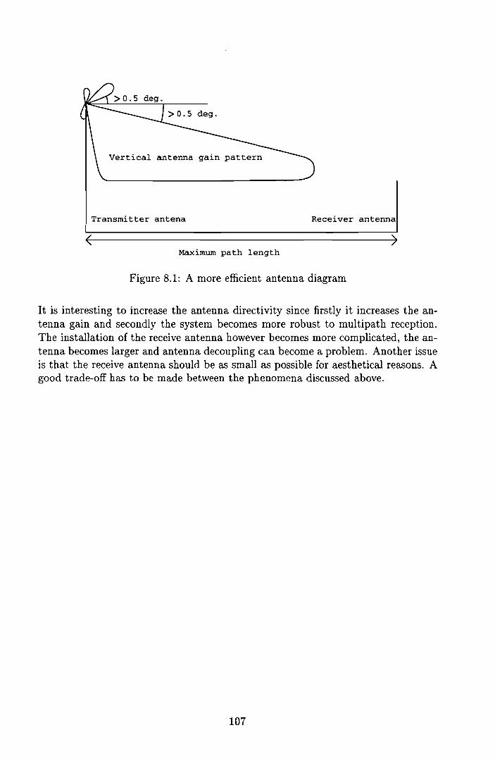
Vertical antenna gain pattern

Transmitter antena

(Maximum path length

Receiver antenna

)

Figure 8.1: A more efficient antenna diagram

It is interesting to increase the antenna directivity since firstly it increases the an­tenna gain and secondly the system becomes more robust to multipath reception.The installation of the receive antenna however becomes more complicated, the an­tenna becomes larger and antenna decoupling cao become a problem. Another issueis that the receive antenna should be as smal1 as possible for aesthetical reasons. Agood trade-off has to be made between the phenomena discussed above.

107

Chapter 9

Acknowledgements

The author would like to thank all the people who have helped carrying out thisresearch work and writing this report. Thanks especially to Ir. P.G.M. de Bot forcoaching and giving technical assistance. Thanks also to Prof. Dr. Ir. G. Brussaardand Ir. J. Dijk from the Eindhoven University of Technology for their assistance inand coaching of this graduation project. The author would like to thank W.J. vanHoutum and ir. H. L. Vermeer for their extensive support in the field trials carriedout for this research project.

Further the author likes to thank Mr. I. Clarke from Philips Microwave for providingtechnical information and support.

108

Bibliography

[1] Strawman specification for digital terrestrial television, March 1995. Draft.

[2] J.C. Arnbak, J. Dijk, M.H.A.J. Herben, and J.T.A. Neessen. Radio en radar.Eindhoven University of Technology, Eindhoven, The Netherlands, 1993. Lec­ture Notes Nr.: 5653.

[3] J.C. Arnbak and W. van Blitterswijk. Capacity of slotted ALOHA in rayleigh­fading channels. IEEE Journal on Selected Areas in Communications, SAC­5(2):261-269, February 1987.

[4] P. Beckmann. Scattering of electromagnetic waves from rough surfaces. ArtechHouse, Inc., Norwood, 1987.

[5] J. Borish. Self contained Crosscorrelation Program for Maximum-length Se­quences. J. Audio Eng. Soc., 33(11):888-891, 1985.

[6] G. Brussaard. A meteorological model for rain-induced cross-polarization. IEEETrans. Antennas and Propagation, AP-24:5-11, January 1976.

[7] J.B. Cain, G.C. Clark, and J.M. Geist. Punctured convolutional codes of rate(n - 1)/n and simplified maximum likelihood decoding. IEEE Trans. Inform­ation Theory, IT-25(1):97-100, January 1979.

[8] T.S. Chu. Rain induced cross-polarization at centimeter and millimeterwavelengths. Bell Systems Technical Journal, 53(8):1557-1579, October 1974.

[9] Commission of the European Communities. Infiuence of the atmosphere oninterference between radio communication systems at frequencies above 1 GHz.Commission of the European Communities, Luxembourg, 1990.

[10] L. M. Correia and P. O. Françês. Estimation of materials characteristics frompower measurements at 60 GHz. In Proc. PIMRC 94 Wireless Networks, TheHague, September 1994.

[11] Robert K. Crane. Prediction of attenuation by rain. IEEE CommunicationsMagazine, 28(9):1717-1732, September 1980.

109

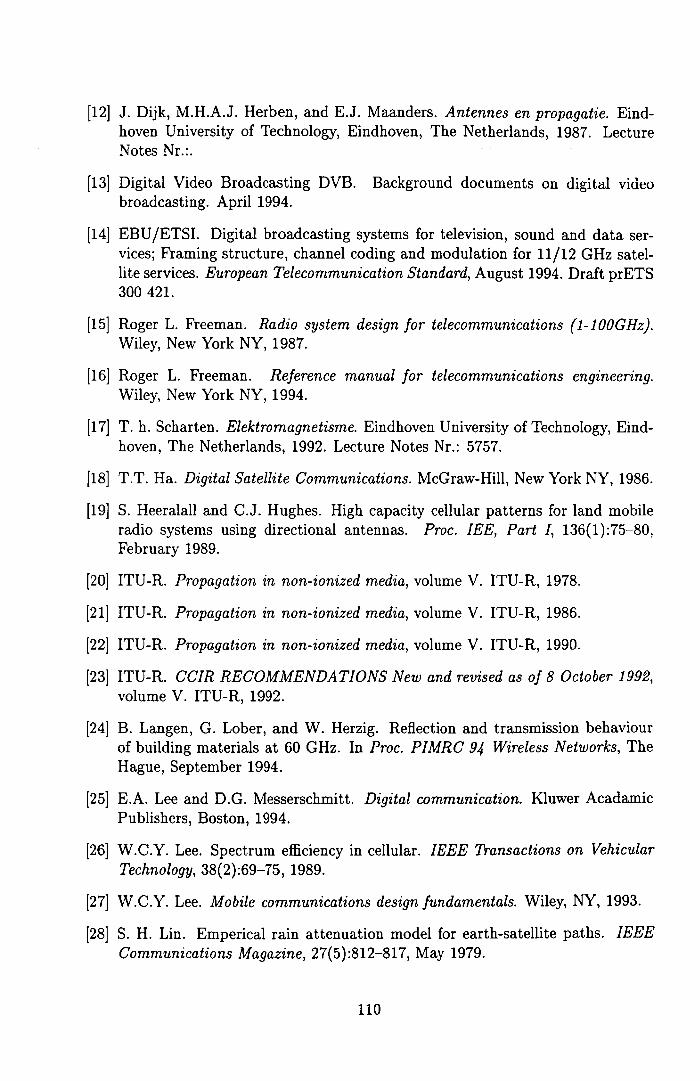
[12] J. Dijk, M.H.A.J. Herben, and E.J. Maanders. Antennes en propagatie. Eind­hoven University of Technology, Eindhoven, The Netherlands, 1987. LectureNotes Nr.:;

[13] Digital Video Broadcasting DVB. Background documents on digital videobroadcasting. April 1994.

[14] EBUIETSI. Digital broadcasting systems for television, sound and data ser­vices; Framing structure, channel coding and modulation for 11/12 GHz satel­lite services. European Telecommunication Standard, August 1994. Draft prETS300421.

[15] Roger L. Freeman. Radio system design for telecommunications (1-100GHz).Wiley, New Vork NY, 1987.

[16] Roger L. Freeman. Reference manual for telecommunications engineering.Wiley, New Vork NY, 1994.

[17] T. h. Scharten. Elektromagnetisme. Eindhoven University of Technology, Eind­hoven, The Netherlands, 1992. Lecture Notes Nr.: 5757.

[18] T.T. Ha. Digital Satellite Communications. McGraw-Hill, New Vork NY, 1986.

[19] S. Heeralall and C.J. Hughes. High capacity cellular patterns for land mobileradio systems using directional antennas. Proc. lEE, Part I, 136(1):75-80,February 1989.

[20] ITU-R. Propagation in non-ionized media, volume V. ITU-R, 1978.

[21] ITU-R. Propagation in non-ionized media, volume V. ITU-R, 1986.

[22] ITU-R. Propagation in non-ionized media, volume V. ITU-R, 1990.

[23] ITU-R. CCIR RECOMMENDATIONS New and revised as of 8 October 1992,volume V. ITU-R, 1992.

[24] B. Langen, G. Lober, and W. Herzig. Reflection and transmission behaviourof building materials at 60 GHz. In Proc. PIMRC 94 Wireless Networks, TheHague, September 1994.

[25] E.A. Lee and D.G. Messerschmitt. Digital communication. Kluwer AcadamicPublishers, Boston, 1994.

[26] W.C.Y. Lee. Spectrum efficiency in cellular. IEEE Transactions on VehicularTechnology, 38(2):69-75, 1989.

[27] W.C.Y. Lee. Mobile communications design fundamentals. Wiley, NY, 1993.

[28] S. H. Lin. Emperical rain attenuation model for earth-satellite paths. IEEECommunications Magazine, 27(5):812-817, May 1979.

110

[29] V.K. Prabhu. Error Rate Considerations for Coherent Phase-Shift Keyed Sys­tems with Co-Channel Interference. BeU 8ystems Technical Journal, 48:743­767, March 1969.

[30] J.G. Proakis. Digital Communications. McGraw-Hill, Singapore, second edi­tion, 1989.

[31] Qualcomm. Q1650 K=7 multi code rate Viterbi decoder, December 1991. Tech­nical data sheet of the Qalcomm Q1650.

[32] P. L. Rice and N. R. Holmberg. Cumulative time statistics of surface point­rainfall rates. IEEE Communications Magazine, 21(10):1131-1136, October1973.

[33] A.S. Rosenbaum and F.E. Glave. An Error-Probability Upper Bound for Co­herent Phase-Shift Keying with Peak-Limited Interference. IEEE Trans. Com­munications, 22:6-16, January 1974.

[34] J. Sarnecki and C. Vinodrai et. al. Microcellular design principles. IEEECommunications Magazine, 31(4):76-82, April 1993.

[35] O. Shimbo and R. Fang. Effects of cochannel interference and gaussian noisein m-ary psk systems. IEEE Trans. Communications, COM-21(10):1108-1115,October 1973.

[36] M.1. Skolnik. Introduction to radar systems. McGraw-Hill, New York NY, 1980.

[37] British Telecommunications. 29 GHz terrestrial microwave systems for satelliteservices. ss6003.

[38] W. v. Houtum. Digital transmission scheme for terrestrial tv, based on theeuropean transmission standard for digital cable tv. Technical report, PhilipsResearch Laboratories Eindhoven, Eindhoven, The Netherlands, January 1995.

[39] J. Vugts. Multipoint video distribution system test setup at philips researcheindhoven. Technical Report 326, Philips Research Laboratories Eindhoven,Eindhoven, The Netherlands, November 1994.

[40] S. Wang and S.S. Rappaport. Signal to interference calculations for corner-excited cellular communications systems. IEEE Trans. Communications,39(12):1886-1895, December 1991.

[41] J.M. Wozencraft and I.M. Jacobs. Principles of Communication Engineering.Wiley, New York NY, 1965.

111

112

Appendix A

Analog system description

A.I Indoor transmit unit

The indoor transmit unit consists mainly of three parts, power supply unit, cableequalization circuitry and the pre-emphasis.

The power supply supplies several dc voltages for the transmitter outdoor unit andmonitors the dc voltages at the outdoor unit. The different supplies are for thevaractor offset, the video amplifiers and the gun oscillator in the outdoor unit.

The cable equalization circuitry provides high frequency tilt to compensate for theattenuation within coax cable from the indoor unit to the outdoor unit. This isexternally adjustable to adapt to the cable length used.

Since the modulation currently used is FM it is common to use pre-emphasis. Thiswill yield a higher signal-to-noise ratio at the receiver. The actual curve used isfound in the recommendation report CCIR 405-1 curve B (625 lines) and shown inFigure A.I.

Figure A.l: Base band pre-emphasis

A.2 Outdoor transmit unit

The outdoor transmit unit consists of a voltage controlled gun oscillator with activeinternal temperature control, a video amplifier and a power supply unit. The FM­sweep (peak-peak) can be adjusted between 10 MHz and 25 MHz. The free runninggun oscillator is directly modulated (varactor-tuned).

Because of the inherent instability of the gun oscillator, a channel spacing of 38.4MHz is required.

113

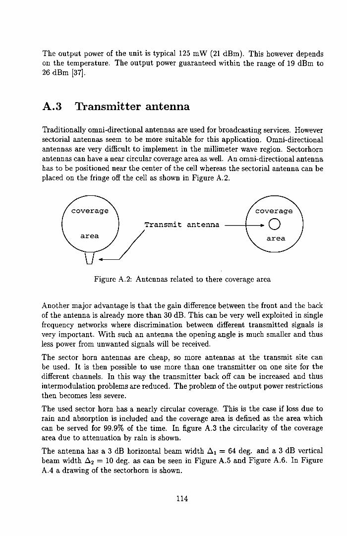
The output power of the unit is typical 125 mW (21 dBm). This however dependson the temperature. The output power guaranteed within the range of 19 dBm to26 dBm [37].

A.3 Transmitter antenna

Traditionally omni-directional antennas are used for broadcasting services. Howeversectorial antennas seem to be more suitable for this application. Omni-directionalantennas are very difficult to implement in the millimeter wave region. Sectorhornantennas can have a near circular coverage area as weIl. An omni-directional antennahas to be positioned near the center of the cell whereas the sectorial antenna can beplaced on the fringe off the cell as shown in Figure A.2.

Transmit antennaareaijFigure A.2: Antennas related to there coverage area

Another major advantage is that the gain difference between the front and the backof the antenna is already more than 30 dB. This can be very weIl exploited in singlefrequency networks where discrimination between different transmitted signals isvery important. With such an antenna the opening angle is much smaller and thusless power from unwanted signals will be received.

The sector horn antennas are cheap, so more antennas at the transmit site canbe used. It is then possible to use more than one transmitter on one site for thedifferent channels. In this way the transmitter back off can be increased and thusintermodulation problems are reduced. The problem of the output power restrictionsthen becomes less severe.

The used sector horn has a nearly circular coverage. This is the case if loss due torain and absorption is included and the coverage area is defined as the area whichcan be served for 99.9% of the time. In figure A.3 the circularity of the coveragearea due to attenuation by rain is shown.

The antenna has a 3 dB horizontal beam width Dol = 64 deg. and a 3 dB verticalbeam width Do2 = 10 deg. as can he seen in Figure A.5 and Figure A.6. In FigureAA a drawing of the sectorhorn is shown.

114

432101234ciSlance trom transmmer. km

Figure A.3: Variation of eoverage area with availahility for a speeifie situation

aperture

/+ 7cm

Figure AA: The seetorhorn transmitter antenna

The isotropic transmitter antenna gain G in dB ean he estimated hy [2]

(27000 )

GdBi = 10 log ~1' ~2 ~ 16dBi

The specified antenna gain is however 15 dBi.

115

(A.1)

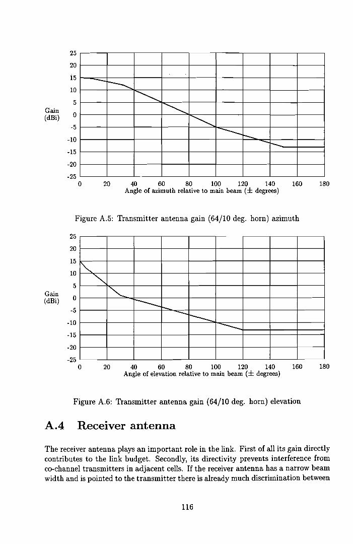
25

20

i5

10

5Gain

0(dBi)

-5

-10

-15

-20

--~~~~ ---.... I--.. -t--...

-25o 20 ~ W M 100 1W 1~

Angle of azimuth relative to main beam (± degrees)160 180

Figure A.5: Transmitter antenna gain (64/10 deg. hom) azimuth

25

20

15

10

5Gain 0(dBi)

-5

-10

-15

-20

'"""""-~r-.. ------ ---

-25o 20 40 60 80 100 120 140 160

Angle of elevation relative to main beam (± degrees)180

A.4

Figure A.6: Transmitter antenna gain (64/10 deg. hom) elevation

Receiver antenna

The receiver antenna plays an important role in the link. First of all its gain directlycontributes to the link budget. Secondly, its directivity prevents interference fromco-channel transmitters in adjacent eells. If the receiver antenna has a narrow beamwidth and is pointed to the transmitter there is already mueh discrimination between

116

the signals of the different transmitters.

A larger antenna increases the antenna gain, however the loss due to incorrect pos­itioning of the antenna also increases. This means that wind gusts may play a roleor the supporting construction becomes complicated, neither of these issues beingvery attractive. Another issue is that the antenna should be as small as possible foraesthetical reasons. A smaller antenna however makes a receiving set more expens­ive because the coverage area becomes smaller, and thus the number of receivers pertransmitter becomes smaller or the noise figure has to be decreased. The smaller theantenna, the cheaper the mechanical support construction is. Thus the installationof the antenna becomes less complicated.

The antenna size must be based on some kind of trade off of the factors discussedabove.

The antenna gain 9r can be calculated with

(1rD) 2

9r = Tl T (A.2)

where Tl is the efficiency, D is the antenna diameter (m) and À is the wavelength(m).

The antenna efficiency is taken to be approximately 0.65. This number is estimatedon common antenna parameters [11]. This yiclds in an antenna gain of 31 dBi at 28

GHz (À = 10.7 mm) and a diameter D = 0.15 m.

For small angles 0, referring to the main beam, the antenna gain pattern can be ap­proximated with a parabolic function. An antenna gain pattern C(O) for a parabolicdish can then be approximated by

C(O)dB = (C(O) - 3 (1.: )2)2 3dB dB

(A.3)

where 03dB is the 3 dB beamwidth which can be calculated with [11] (parabolic).

whereD = antenna diameter (m)À = the wavelength (m).

O_ 72.7· À

3dB - D(AA)

If the antenna is misaligned by installation or due to the wind, the main lobe willnot be pointed exactly to the transmitter. This results in a pointing loss. With d =0.15 mand À = 10.7 mrn, we get a beam width 03dB of approximately 5 deg. Withformula A.3 the pointing loss can be determined. For small pointing deviations ofthe antenna the loss will be very low or negligible.

117

A.5 Outdoor receive unit

The outdoor receive unit consists of5 parts, the RF band pass filter, local oscillator,the mixer, IF amplifier and a power supply. In Figure A.7 the block diagram isshown.

Mixer

Band pass

Filter

Power

supply

Local

oscillator

Figure A.7: The block diagram of the outdoor unit

The RF filter has a pass band of 800 MHz centered at 28.5 GHz. This filter givesan image rejection of not less than 35 dB. The local oscillator runs at a frequency of27.375 GHz (± 1 MHz) which mixes the RF signa! to the L-band. The IF amplifieramplifies the signal to an acceptable value for the indoor receive unit (-60 to -20dBm) depending on the receive level. The system noise figure up to the low noiseblock equals 10 dB.

A.6 Indoor receive unit

The indoor receive unit is currently a standard satellite tuner. It uses a bandwidthof 27 MHz and is tunable over the L-band from 950 MHz to 1750 MHz. The tuneruses a PLL to demodulate the FM signal yielding an FM threshold of 8 dB. In FigureA.8 the threshold effect is shown. In this figure the signal-to-noise ratio is plottedversus the carrier-to noise ratio. The noise generated by this module is included inthe noise figure of the outdoor receiver.

Figure A.8: signal-to-noise ratio versus carrier-to-noise ratio

118

Appendix B

Power decay rate

For "low" frequencies (1 GHz) the power decay rate in urban areas is of the order of4 instead of 2. In this section we will show that this is not the case for frequenciesused in the MVDS systern.

If it is assumed that the ray bearns obey the rules of optical refiection, no refraction,the received field strength with one refiection is given by the following formula asshown in Section 3.5.

(B.1)

where kt is the transmitter height, k r is the receiver height, >. is the wave lengthand d is the path length.

This is under the assumption that the distance d is rnuch larger than the heights ofthe antennas and thus the refiection coefficient p = -1. Further we assume a totallyfiat earth (k = 00).

Now for very large wave lengths >. the product>' . d is rnuch larger than 2· 1r • htkr .

Then we approximate the sin(x) with the first term of the taylor series x. This yields

~ = ,41rkr k t )1Eo >.. d

(B.2)

Since the field strength Eo is inversely proportional to the distance d, an electromag­netic wave is a spheric wave, the received field strength E is inversely proportionalto d2• Since the power is direct proportional to the square of the received field Ethe received power is then proportional to 1/d4 .

For the frequency of 42 GHz however this is not true because >. . d is at most inthe order of 7.14 . 10-3 • 10· 103 = 71.4. If we assume a transmitter height of morethan 50 mand a receiver antenna height of approximately 10 m one can see that theseries approximation for the sine function is not valid. The received field strengthwill then maintain its sinusoidal behaviour as a function of the distance d. Thus thepower decay rate of 4 due to a refiection will not be the case.

119

If the first Fresnel zone is not completely free from obstruction the received fieldstrength reduces as we have seen in Chapter 3.3. This partially obstructing of theFresnel zones introduces extra attenuation which depends on the type of obstructingstructures. In an urban area the first Fresnel zone can easily be obstructed withbuildings etc. This results in a statistical average power decay rate which is largerthan 2 in an urban area.

The radius of the Fresnel zone is given by

(B.3)

whereRn = the radius of the nth Fresnel zone (m)dl and d2 are the distances from a point in the radio path to the antennas (km)f = the used frequency (Hz).

One can see that for decreasing frequency the radius of the Fresnel zone increases andalso increases if the path length is increased. This means that for links using lowerfrequencies and larger path lengths the first Fresnel zone becomes easily obstructed.

In the short 42 GHz links the Fresnel zones become very smalI, thus it is much easierto keep the first Fresnel zone free from obstruction. As an example the maximumradius of the first Fresnel zone at a 42 GHz link of 5 km equals 2.98 mand witha 1 GHz path of 50 km this equals 61.16 m (19.34 m for a path of 5 km). A 42GHz link is entirely based on a LOS, it is thus assumed that at least half of thefirst Fresnel zone is free of obstruction throughout the entire path. . Since theelectromagnetic waves are spheric the free space loss is due to the spheric expansionand thus proportional to 1/d2•

120

Appendix C

Snellius law for a round earth

From the definition of the refractivity index and the fact that it decreases withaltitude it follows that the travelling speed of the waves increases with increasingaltitude [2]. This results in a curved ray path. Measurements have shown that therefractivity index doesn't change too much in the horizontal direction. It is thereforeallowed to look at the problem as if the atmosphere is divided into spherical layers.

o

Figure C.l: Ray path through a spherical atmosphere[2]

121

In figure [2] C.1 we see the earth with part of its atmosphere. From this figure weean see that

11.0 sin 1/Jo = 11.1 sin 1/J~

11.1 sin VJ1 = 11.2 sin 1/J~

If we multiply these with the different radii we get

11.0 • TO sin 1/Jo = 11.1 • TO sin?p~

Sincesin(7r - 1/JD sin ?PI

Tl TO

we get11.0 • TO sin '!/Jo = 11.1 • Tl sin 1/J1 = 11.2 • T2 sin 1/J2 = ...

As a result we have

11. • T sin 1/J = 11.0 • ro sin 1/Jo = constant.

Figure C.2: Model to calculate the curvature p[2]

(C.1)

(C.2)

(C.3)

(CA)

(C.5)

(C.6)

(C.7)

To calculate the actual curvature of a radio beam we proceed as follows. We taketwo spherical layers very near to each other (Figure C.2) [2]. From AB there istravelling a wave front of the beam. The phase speed at point B ds' is higher than

122

the phase speed ds at point A. Suppose ds = v and ds' = v + dv. This yields thefollowing equations:

This leads to

d'lj; vds = p . d'lj; = v . dt --+ - = -

dt P

, ~ v+~ds = (p + dp) . d'lj; = (v + dv) . dt --+ - =--

dt p + dp

(C.S)

(C.9)

(C.1D)dv dpv p

where p = ds/d</> is the radius of curvature of the curve AA'.

According to the definition of the refractivity index n the velocity v of the travelingwave through the medium is defined as

cv= ­

n

where cis the velocity of an electromagnetic wave in a vacuum.

The derivative of the speed related to the refractivity yields

(C.l!)

dv cdn n2

dvv

dnn

vn

(C.12)

(C.13)

Using (C.lD) we get

From Figure C.2 we can see that

1

p

1 dn---

ndp(C.14)

dh ~ dpcos('Ij;) (C.15)

With terrestrial transmission the angle 'Ij; almost equals D. Assuming the refractivityalmost 1 results in the following equation

1 dn(h)-~--

p dh(C.16)

where n(h) is the refractivity as a function of height.

The curvature of the ray heam can now he calculated if the function n(h) is known.

There are two common models to describe the curvature of the ray beam. Themodel described here is the k-factor model. In this model it is assumed that theray beam follows a straight path. The curvature I/pis then accounted for in theeffective earth radius ae as shown in Figure C.3.

123

radio beamradio beam

ear~1---.-=f~--r,=",""__

Figure C.3: Earth radius a and effeetive earth radius ae in the k-faetor model

From this figure the next equation ean he derived[2]

1 1 1

a p ae(C.17)

where I/ais the eurvature of the earth, I/pis the curvature of the radio heam and1/ae is the effective earth curvature.

The relative curvature hetween the earth and the radio heam in Figure C.3 is keptconstant. The k-factor is now defined as

k = ae

a

Now it can he eoncluded that

k __l_~ 1- 1-! 1 + a dn

p dh

and using the refractivity this yields in

k- 1- 1 + a dn • 10-6

dh

(C.IB)

(C.19)

(C.20)

With this formula the k-factor ean he calculated and thus the effeetive earth radiuscan he calculated.

124

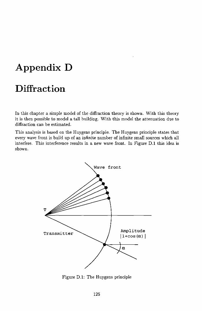
Appendix D

Diffraction

In this chapter a simple model of the diffraction theory is shown. With this theoryit is then possible to model a tall building. With this model the attenuation due todiffraction can be estirnated.

This analysis is based on the Huygens principle. The Huygens principle states thatevery wave front is build up of an infinite number of infinite small sources which allinterfere. This interference results in a new wave front. In Figure D.1 this idea isshown.

TransmitterAmplitude11+cos(<x) I

Figure D.1: The Huygens principle

125

In Figure D.2 the setup of the transmitter and receiver is shown. For very smallangles {3 the setup is simplified as shown.

T R

Transmitter Receiver

front

~ Small angles~

Receiverd2dl

Transmitter

T R

wave front

Figure D.2: Transmitter and receiver configuration

According to Kirchoff the electric field E on the surface S is proportional to thereciprocal of the distance PI from the source T to the surface S.

(D.1)

For small angles {3 the received field in R can be approximated with Kirchoffs law

(D.2)

where A is an arbitrary constant.

If the distance between the receiver and the transmitter is large, {3 very small, theelectric field can be approximated by

(D.3)

126

R

(D.4)

Figure D.3: A two-dimensional model

A two-dimensional model is presented in Figure D.3. In this model an infinite longline source is assumed. An obstacle is now idealized as an infinite long surface witha sharp edge to simplify calculations. This model yields usable results [2].

The phase 4J of the received electric field is given by

271"4J = T(PI + P2)

The distance PI can be approximated with

(D.5)

This results in a phase relation like

(D.6)

Now we are only interested in the phase difference so

and thus

E f"V A' { exp (j .~ .8 2 (..!- + ..!-)) d8is À dl d2

Introducing a new variabie 1/

the electric field can be written as

E f"V A" Is exp (j%.1/2) d1/

127

(D.7)

(D.8)

(D.9)

(D.lO)

(D.U)À=h·

If the electromagnetic field is obstructed as depicted in Figure D.3 it is necessaryto set the integration limits from the obstacle hight h to infinity. The limit infinitycomes in very handy and is allowed because the contributions to the received electricfield in R for large diffraction angles becomes zero. If we set À to

2 1 1-X(dl + d

2

the received field can be written as

100 1r

E rv A" exp(j _1/2) d1/l1 2

(D.I2)

This equation can be expanded as

{ 111 1r 1111rE rv A" - cos( - . 1/2) d1/ - j sine - . 1/2) d1/ +

o 2 0 2

100 1r 1001r }cos( - . 1/2) d1/ + j sine- . 1/2) d1/

o 2 0 2

(D.I3)

Since[00 cos(ax2 ) dx = [00 sin(ax2 )dx = ! .~

Jo Jo 4 athe electrical field becomes

E rv A" . (~(1 + j) - [C(À) + j . S(À)])

where C(~) and S(À) are the eosine and sine Fresnel integrals defined as

C(À) = [11 cos(~ . 1/2) d1/Jo 2

(D.I4)

(D.15)

(D.I6)

and[11 7r

S(À) = Jo sin("2' 1/2) d1/

The free space electrical field strength is given by

Eo = A" JOO exp(j~ . 1/2) d1/ = A" . (1 + j) = A"J2· ëi-00 2

therefore the attenuation due to shielding can be estimated with

(D.I7)

(D.I8)

E eii (1 )Eo = v'2' 2(1 + j) - (C(À) + j. S(~))

and the loss L df due to diffraction is thus given by

Ldf = 20 * log (1~J2· [~(I + j) - (C(À) + j. S(~))] I)

(D.I9)

(D.20)

with

~=h·2 1 1_.(-+-)..\ dl d2

(D.2I)

128