Eindhoven University of Technology

MASTER

Measurement of coal particle-size in shock-tube experiments using laser Mie-scattering

Commissaris, F.A.C.M.

Award date:1992

Link to publication

DisclaimerThis document contains a student thesis (bachelor's or master's), as authored by a student at Eindhoven University of Technology. Studenttheses are made available in the TU/e repository upon obtaining the required degree. The grade received is not published on the documentas presented in the repository. The required complexity or quality of research of student theses may vary by program, and the requiredminimum study period may vary in duration.

General rightsCopyright and moral rights for the publications made accessible in the public portal are retained by the authors and/or other copyright ownersand it is a condition of accessing publications that users recognise and abide by the legal requirements associated with these rights.

• Users may download and print one copy of any publication from the public portal for the purpose of private study or research. • You may not further distribute the material or use it for any profit-making activity or commercial gain

Faculty of Electrical Engineering

Division Electrical Energy Systems

Measurement of coal particle-sizein shock-tube experimentsusing laser Mie-scattering

F.A.C.M. Commissaris

The Faculty of Electrical Engineering of theEindhoven University of Technology doensn'taccept any responsibility for the contentsof this report.

Supervising scientist:Dr. A. VeefkindEindhoven, July 1992

EINDHOVEN UNIVERSITY OF TECHNOLOGY

EG/92/605

Acknowledgements

First, I want to thank dr. Veefkind for giving the opportunity for this work and for his

inspiring and able coaching. Further, I wish to express my gratitude to Valentina Bajovic

B.Sc., for her valuable proposals concerning the experimental set-up. Finally, thanks to

the people who helped constructing the devices necessary for the experiment.

7 rank Comrnissa:~~

"Mehr Licht I"

(Goethe's last words)

Summary

In the study of chemical reactions that determine the combustion and gasification of

coal-particles inside a shock-tube, one wishes to know the size of these particles. This

size changes during combustion process. A way of determining this particle-size, is the

measurement of the intensity of laser light that is scattered by the particles. This

intensity is determined by the mean particle-size, among other physical parameters. The

theory that relates the size of a single particle to its scattering of light to different

angles, is first described by Mie. The purpose of this work concerns the implementation

of this theory in computer programs as well as its experimental application.

Mie's equations for scattered light intensities contain certain special mathematical

functions, often having complex arguments. For these functions, convenient recurrence

relations are derived, that make fast computations of the so-called Mie-intensity­

functions possible. Further, an experimental set-up to measure scattered light intensi­

ties is made. The dimensions of the optical part of set-up are determined according to

rules of geometrical optics, in such a way that Mie-theory can be applied to the experi­

ment.

Scattered light intensities are measured, but this appears to be impossible during

combustion of the particles, due to intense light emission. Comparing the scattered

light intensity ratios found after the experiment to computational values, a certain

effective particle-radius is extracted, that is comparable to the assumed geometrical

radius.

In further experiments, the use of monochromators will be necessary. In this case, a

smaller region in the spectrum of the emission light will be considered. Also a stronger

laser has to be used to make the desired measurements possible. The intensity of this

laser depends upon the spectral resolution of the monochromators that will be used.

The higher the intensity of scattered light compared to the intensity of emission light,

the more accurate the measurements. Finally, in this work other suggestions are

presented concerning the set-up of the experiments, in order to carry them out more

accurately.

List of symbols

The most important symbols used in this work are:

intensity of scattered light

intensity of incident light

,'max

() , (/)

n

q

N

Mie-intensity-functions

complex amplitude-coefficients

index of partial wave and term in Mie-series

maximum number of terms in Mie-series

spherical coordinates, determining the plane of observation

complex refractive index

wavelength of incident and scattered light

size parameter

particle radius

count median radius

geometric standard deviation

expectation of particle-radius

number of particles

concentration of particles

distance between scattering volume and detector

scattering volume

diameter of apertures.

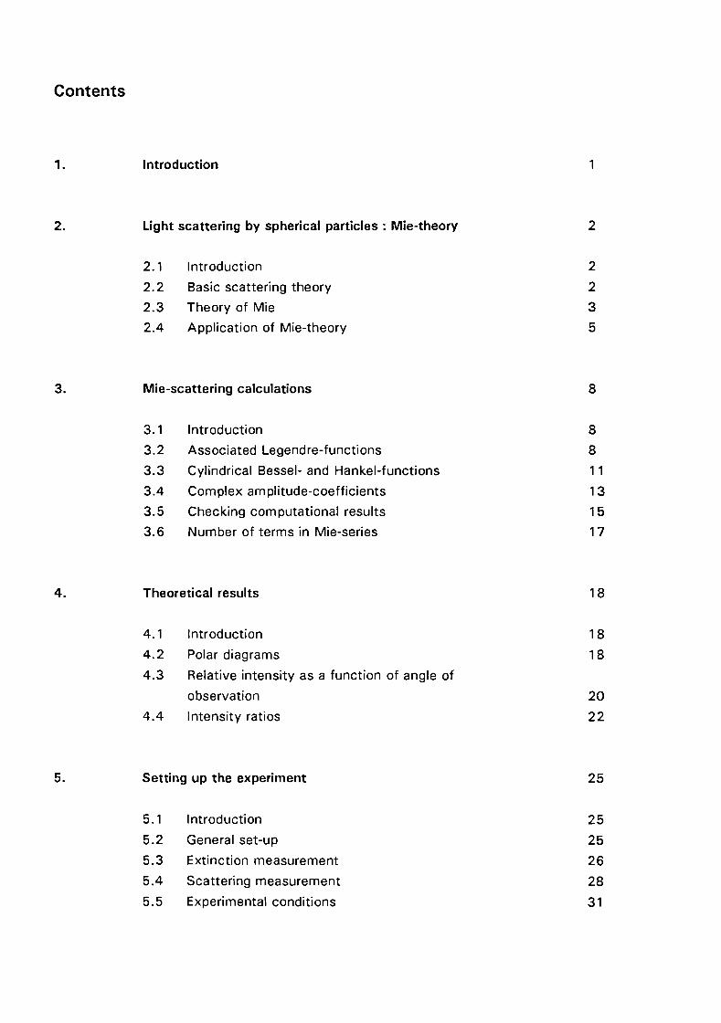
Contents

1.

2.

Introduction

Light scattering by spherical particles: Mie-theory

1

2

2.1

2.22.32.4

Introduction

Basic scattering theory

Theory of Mie

Application of Mie-theory

2

2

35

3. Mie-scattering calculations 8

3.1

3.23.33.4

3.53.6

Introduction

Associated Legendre-functions

Cylindrical Bessel- and Hankel-functions

Complex am plitude-coefficients

Checking computational results

Number of terms in Mie-series

8

8

1 1

13

15

17

4. Theoretical results 18

4.1

4.2

4.3

4.4

Introduction

Polar diagrams

Relative intensity as a function of angle of

observation

Intensity ratios

18

18

20

22

5. Setting up the experiment 25

5.1

5.25.35.4

5.5

Introduction

General set-up

Extinction measurement

Scattering measurement

Experimental conditions

252526

28

31

6. Experimental results and discussion 32

6.1

6.26.3

Introduction

Experimental results

Discussion

323233

7. Conclusions

8. References

Appendix 1 Dispersion model

Samenvatting

38

39

41

43

Chapter 1 Introduction

The students of the Electrical Engineering faculty at the Eindhoven University of

Technology finish their study with a final traineeship. This work takes about six months

and its subject must be in some way related to Electrical Engineering. The purpose of

all this, is that the students expand and apply the knowledge they have developed so

far. The project takes place at a group of the faculty, and is supervised by a senior

scientist.

In the Electric Energy Systems group, research is done in the field of coal-combustion

and -gasification. For this purpose, a shock-tube is available, with which the desired

conditions can be established for the combustion of coal particles. The high tempera­

ture necessary for combustion, is reached after adiabatic compression of a test gas, for

example 02'

Some of the chemical reactions during combustion take place on the surface of the coal

particles. To study these reactions, information on the particle size is desired. The

method to determine the mean particle size, is based on light scattering. The light of a

laser beam is scattered by the coal particles in many directions. Because coal particle

size, among other physical parameters, determines the scattered light intensity, the

required information of the coal particles can be obtained by measuring this intensity at

different angles. The theory that provides the theoretical intensities, is developed by

Gustav Mie (1908).

In this work, the results of the Mie-theory are presented and implemented in computer

programs. Recurrence formulae for special mathematical functions contained in the so

called Mie-intensity-functions are derived in such a way that calculations are efficient

and fast. Then the experimental set-up is described, following the constraints of the

Mie-theory and rules of geometrical optics. Finally, a comparison is made between

theoretical and experimental results, and suggestions are given for further research in

this field.

1

Chapter 2 . Light scattering by spherical particles Mie-theory

2.1 : Introduction.

This chapter deals with light scattering in general and Mie-theory, the theory on which

the experiments are based, in particular. First, a few basic ideas and definitions

concerning light scattering will be outlined. Then the mathematical results of the Mie­

theory will be presented, followed by its application for the shock-tube experiments.

2.2 : Basic scattering theory. [1]

Most of the light we see is scattered light, we hardly ever observe light directly from its

source. Scattering can be seen as an interaction between incident light and the

scattering object. The removal of energy from an incident light wave and the subse­

quent reemission of a certain portion of that energy, is known as scattering. It is the

underlying physical mechanism operative in reflection, refraction and diffraction.

Scattering is often accompanied by absorption, a phenomenon that also causes a

removal of a portion of the incident energy. The total removal of energy from a beam of

light, caused by scattering and absorption, is called extinction. Using this terminology,

we can put:

extinction = scattering + absorption

A lot of examples concerning scattering can be given, some more impressive than

others, but just the ability to read this page is a result of scattering. A famous example

of a scattering phenomenon, concerns the blue color of the sky. Rayleigh has shown

that almost all light seen in a clear sky is due to molecular scattering by the air

molecules. If this scattering would be absent, a cloudless sky would appear completely

black, except in the direction of the sun. This case of scattering, for which the particles

(in fact molecules) are very small compared to the wavelength, is therefore called

Rayleigh-scattering. It is found that the scattered intensity in this case is proportional to

the square of the volume of the particle and to 1 over the wavelength to the fourth

power. Thus the scattering of blue light is about ten times as great as the scattering of

red light. Another example is the smoke rising from the lighted end of a cigarette; this

smoke is made up of particles that are smaller than the wavelength of light, and so it

appears blue to us.

2

Closer related to the subject of this work, is the scattering of light by particles with a

size comparable to or greater than the wavelength of light. The scattering of light by

particles much greater than its wavelength, is more or less independent of the wave­

length. A beam of sunlight entering a room, is made visible to us by the white light

scattered by the dust particles in the air.

Gustav Mie in 1908 published a mathematical solution for scattering from a sphere of

both arbitrary radius and index of refraction. Note that his theory is dealing with a

single sphere. The last paragraph of this chapter will deal with the assumptions which

have to be made in order to make Mie-theory applicable for clouds of particles.

2.3 : Theory of Mie.

Detailed descriptions of Mie-theory can be found in [11 and [21. The terminology used in

this chapter can be considered as a combination of those used in these two works.

Basically, Mie-theory is a solution to a set of Maxwell equations. These equations are

applied to a field arising from a plane, monochromatic wave incident upon a spherical

surface, across which electromagnetic properties of the medium change abruptly. A

rectangular system of coordinates is taken, with the origin at the center of the sphere.

As fig.2.1 shows, the wave propagates in the z-direction and has its electric vector pi}

in the x-direction.

x>

direction of propagation

z

fig.2.1 : Diffraction by a conducting sphere.

3

In the Maxwell equations and boundary conditions, the assumptions are made that the

medium surrounding the sphere is non-conducting, and that there is zero current- and

charge-density on the surface of the sphere. Further, the wavelength of the scattered

light is assumed to be the same as the wavelength of the incident light.

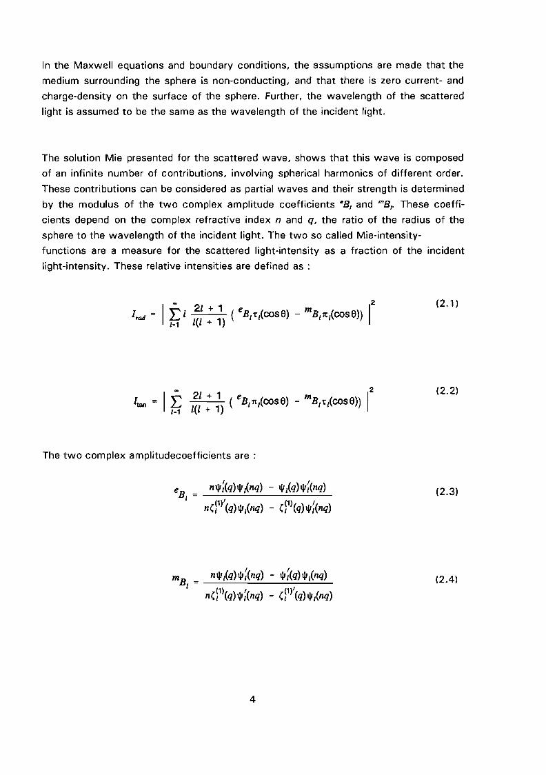
The solution Mie presented for the scattered wave, shows that this wave is composed

of an infinite number of contributions, involving spherical harmonics of different order.

These contributions can be considered as partial waves and their strength is determined

by the modulus of the two complex amplitude coefficients eB, and mB,. These coeffi­

cients depend on the complex refractive index nand q, the ratio of the radius of the

sphere to the wavelength of the incident light. The two so called Mie-intensity­

functions are a measure for the scattered light-intensity as a fraction of the incident

light-intensity. These relative intensities are defined as :

~ 2

1

",,·21+1 e ( ) m 1I,atI = L l ( B1", cas 6 - B,1t,(coS6))'=1 1(1 + 1)

The two complex amplitudecoefficients are:

e nt,,:(q)tJI,(nq) - tJI,(q)tJI:(nq)B, = -~----=---------=-_--:....._-

n(}1)/(q) tJI,(nq) - d1)(q) tJI:(nq)

ntJI,(q) tJI:(nq) - tJI:(q) tJI,(nq)

n(p)(q)tJI:(nq) - (~1)/(q)"'I(nq)

4

(2.1)

(2.2)

(2.3)

(2.4)

In these formulae, the size parameter q is defined as

21tq = - r1 p

where A is the wavelength of the incident light and f p stands for the radius of the

sphere. Further, the special functions which appear in the formulas above, are:

p11)(cos 6)

1t,(cos6) = ---:...._-­sin6

',(cas6) = pf)'(COS6)sin6

(1) r-;; (1) )(, (p) = ~ 2 H'.1/2(P

(2.5)

(2.6)

(2.7)

(2.8)

(2.9)

In these definitions, P/IJ(cos 8) is the associated Legendre-function of the first order,

J,+ 1I2(P) a Bessel-function and H'IJ,+ lIip) a Hankel-function of the first kind. The use of

the accent implies differentiation of the function with respect to its argument. These

special functions and their first derivatives are the subject of chapter 3, where recurren­

ce formulae will be derived, which are convenient for (fast) computation.

2.4 : Application of Mie-theory.

In the previous section, light scatttering by a single particle was considered. Before the

formulae can be applied to a cloud of coal particles, a few essential assumptions have

to be made. First, we have to take notice of the fact that the coal particles are far from

spherical and also have a great inner surface.

5

Therefore, it is better to consider the outcome of a light-scattering measurement as an

effective particle size, rather than the geometrical particle size. This effective particle

size is in fact the particle size in the case of spherical particles, causing the same

scattering intensity ratios as the measured ones, that were caused by the non-spherical

coal particles. Important is, that the effective particle size has a meaning which is

practical for the combustion experiments. Detailed research on the influence of particle

shape would be beyond the scope of this work.

One limitation is, that independent particles are considered. If the particles are suffi­

ciently far from each other, there is no interference between light scattered by different

particles to the same detector. For this purpose, the mutual distances between the

particles should be much greater than the wavelength of the incident light.

A second limitation is that effects of multiple scattering are neglected. Each particle is

also exposed to light scattered by other particles. If this effect is so weak that it can be

excluded, one speaks of single scattering. This has a very important consequence: the

intensity of light scattered in a volume containing N scattering particles, is N times the

intensity of light scattered by a single particle. A simple test for the absence of multiple

scattering can be the extinction. If the intensity of the incident beam after passing the

coal-cloud is at least 90% of its original value, single scattering prevails, and we can

use the simple proportionality described above.

If 10 is the intensity of the incident light (watt/m 2) and R is the distance from the center

of the sphere to the point of observation, the resulting intensity of light scattered by a

single sphere, in case of polarized incident light, will be :

(2.10)

Together with the other spherical coordinate 8, (/) determines the direction (8,(/)) of

observation. When (/) = (T/2 or (/) =0, the scattered light is linearly polarized. In the case

of natural light, the appropriate formula for the resulting intensity can be obtained from

(2.10) by averaging over all directions of polarization, and this yields:

6

I'ad + l tan

2(2.11)

Formula (2.13) on page 7 should be :

ERRATUM

(2.13)

For No particles in the scattering volume. taking into account the distribution of the

particle-size. the resulting intensity will be

(2.12)

where R now stands for the distance between the scattering volume and the detector.

The probability-density function of the particle-radius. f(fp ). is assumed to be the log­

normal-distribution :

1 [ (In r p - In r pg)2)j(r) = --- exp - ...l...-...!:....-_~!-

/2itrpog 2 (Inog)2

(2.13)

In this formula. f pg is the count median radius and ug stands for the geometric standard

deviation. For this distribution. the expectation of particle-radius is :

(2.14)

Because it is very difficult to measure absolute intensity. we are interested in the ratios

of intensities of light scattered to different angles 8. If in our experiment the ratio of No

and W can be kept constant for every 8. we have:

(2.15)

J(IraJ.62 + l tan•6a) j(rp)drpr,=O

This ratio is a function of the known parameters II, 8 1 and 82 and of the unknown

parameters n, ug and fpg- If intensity is measured at an adequate number of angles.

these unknown parameters can be found solving the reversed problem and the

expectation of particle-radius is found using (2.14).

7

Chapter 3 Mie-scattering calculations

3.1 : Introduction.

In the previous chapter, we encountered some special mathematical functions. Before

one is able to make fast Mie-scattering calculations, it's necassary to have convenient

recurrence formulae for these functions. Otherwise, the calculation of the integrals in

(2.15) would be very time-consuming. In this chapter, definitions and recurrence

formulae for the special functions will be given, based on previous investigations in [3].

Furthermore, the formulae (2.3) and (2.4) will be "rearranged" for faster computation.

Finally, the checking of computational results and the necessary number of terms in the

Mie-series of (2.1) and (2.2) will be discussed.

3.2 : Associated Legendre-functions.

In the Mie-intensity-functions of the previous chapter, we found terms containing the

associated Legendre-function and its derivative:

p11)(coS6)

sine(3.1)

The Legendre-polynoms in x are defined as

MPl(x) = L (-1)m (21-2m)1 xl -2m

m-a 21ml(l-m)I(I-2m)1

(3.2)

(3.3)

where M =1/2 if 1 is even and M = (1-1 )/2 if 1 is odd. With this pOlynom, the associated

Legendre-functions of order m are defined :

(3.4)

8

We are dealing with the case for which m = 1 and x =easB.

To derive a recurrence formula for (3.1) we use a recurrence formula for the associated

Legendre-functions [4] :

p(1)(cose) = case 2/-1 p~)(cose) - _I_p~)(cose)1 1_1 11 1_112

Simply dividing all terms by sinB, gives us the desired expression :

(3.5)

(3.6)

To avoid unnecessary calculation-time, we will seek an expression for TleasB) in terms

of "leasB), "/-,teasB) etc. It is shown in [3] that:

(3.7)

Using definitions (3.1) and (3.2), a first expression for TleasB) is found:

(3.8)

For the Legendre-polynom in this formula, the following recurrence relation holds:

2/+1 1Pl+1(X) = x--P1(x) - -Pl-1(x)

1+1 1+1

Differentiation on both sides yields :

dP1+1(X) = 21+1 [x dP1(x) + P,(X») __I- dPl_1(X)dx 1+1 dx 1+1 dx

With definition (3.4) we find:

P() _ 1 (1+1 p(1)() p(1)() 1 p(1)(»)I x - -- 1+1 X - X 1 X + -- 1-1 Xb-x2 21+1 21-1

9

(3.9)

(3.10)

(3.11)

Substituting x = cas(} and using (3.1) gives us

1+1 1P,(cos6) = --1t/+1(cos6) - cos61t,(cos6) + --1t,_1(cos6)21+1 21+1

where "I+,(cas(}) can be determined incrementing all indices in (3.6) by 1.

Finally, we obtain:

The desired recurrence formula is found combining (3.8) and (3.13) :

't,(cos6) = -Icos 61t,(cos6) + (1 + 1) 1t/-1 (cos 6)

(3.12)

(3.13)

(3.14)

In calculations on the computer, one must be careful when using (3.6) and (3.14) for all

I, because of possible division by zero. Furthermore, we need initialisation terms to

start the recurrence process. For 1< 1 we have:

1t,(coS6) 1,<1 = 't,(cos6) 1,<1 = 0 (3.15)

For the purpose of finding initialisation terms, the following formula [41 is convenient

(because taking 1= 1 in (3.6) would yield division by zero) :

M

:It,(oos6) = E (21-4r -1)P'_2r_1(oos6)r=O

where M = (1-1 )/2 if (1-1) is odd, M = (1-2)/2 if (1-1) is even.

For 1= 1, (3.16) yields:

Finally, using (3.14), another initialisation term is found:

10

(3.16)

(3.17)

(3.18)

3.3 : Cylindrical Bessel- and Hankel-functions.

These special functions occur in the complex amplitude coefficients, defined by (2.3)

and (2.4). Note that the cylindrical functions have complex arguments, because the

product nq is complex. As in the previous paragraph, the purpose is to find recurrence

relations which enable us to make fast computations.

For all values of k, the Bessel-function is defined as :

. ( )27-1J = -1 r 1 £.t(p) ~ ( ) rlr(r-k+1) 2

The Neumann-function can be written as :

Together, they form the Hankel-function of the first kind:

(3.19)

(3.20)

(3.21 )

Note that this function is complex, even if its argument p is real, where as (3.19) is real

for any real argument. The cylindrical Bessel- and Hankel-functions have the form:

(1) r;; (1)(, (p) = ~ 2 H,+1/2(P)

11

(3.22)

(3.23)

Recurrence formulae for both functions and their derivatives are developed in [3] :

21-1!I(p) = --h-1 (p) - h-2(P)

p(3.24)

(3.25)

In these relations, f/p) can be either tp/p) or ~(1)(p).

Looking at formulae (2.3) and (2.4), we see that the expressions for the complex

amplitude coefficients could be simplified by dividing all terms by tp/nq). Therefor,

Bohren [5] suggests the introduction of a new complex function:

.t:(p)=--

!I(p)(3.26)

For this function, a recurrence relation has to be derived. Dividing all terms in (3.25) by

f/p) and decrementing index I by 1, gives us :

1-1- --p

(3.27)

Using equation (3.24) to eliminate fI-2 (p), we find:

DI- 1(P)1= -p

h(P)---h-1(P)

(3.28)

Finally, after using (3.25), (3.26) and (3.28), the desired expression is found:

D1(p) =__1__

1- - DI- 1(P)p

1p (3.29)

The use of this new complex function shall be discussed in the following section,

where the complex amplitude-coefficients will be rearranged for computation purposes.

12

3.4 : Complex amplitude-coefficients.

Using (3.26) for the cylindrical Bessel-functions, equations (2.3) and (2.4) can be

rewritten as :

eB1

:;:: (3.30)

(3.31 )

Examining these formulae, two advantages are visible. First, we see that there are no

longer derivatives of the cylindrical functions present in the new expressions. Second,

the remaining cylindrical Bessel- and Hankel-functions no longer have a complex

argument, but instead there is only one function with a complex argument, D/nq). The

advantage in calculation time lies in the fact that in the computations no longer special

functions have to be called, that deal with arithmetic operations on complex numbers.

This second advantage also has a consequence from the mathematical point of view.

Combining equations (3.20) and (3.21), using k =/+ 1/2, the Hankel-function of the first

kind can be written as :

(3.32)

In the case of a real argument p in (3.22), (3.23) and (3.32), we find that the real part

of the cylindrical Hankel-function is in fact the cylindrical Bessel-function. Thus we can

state (a is real) :

(3.33)

The introduced function x/a) is also real and satisfies a recurrence-relation similar to

(3.24) :

13

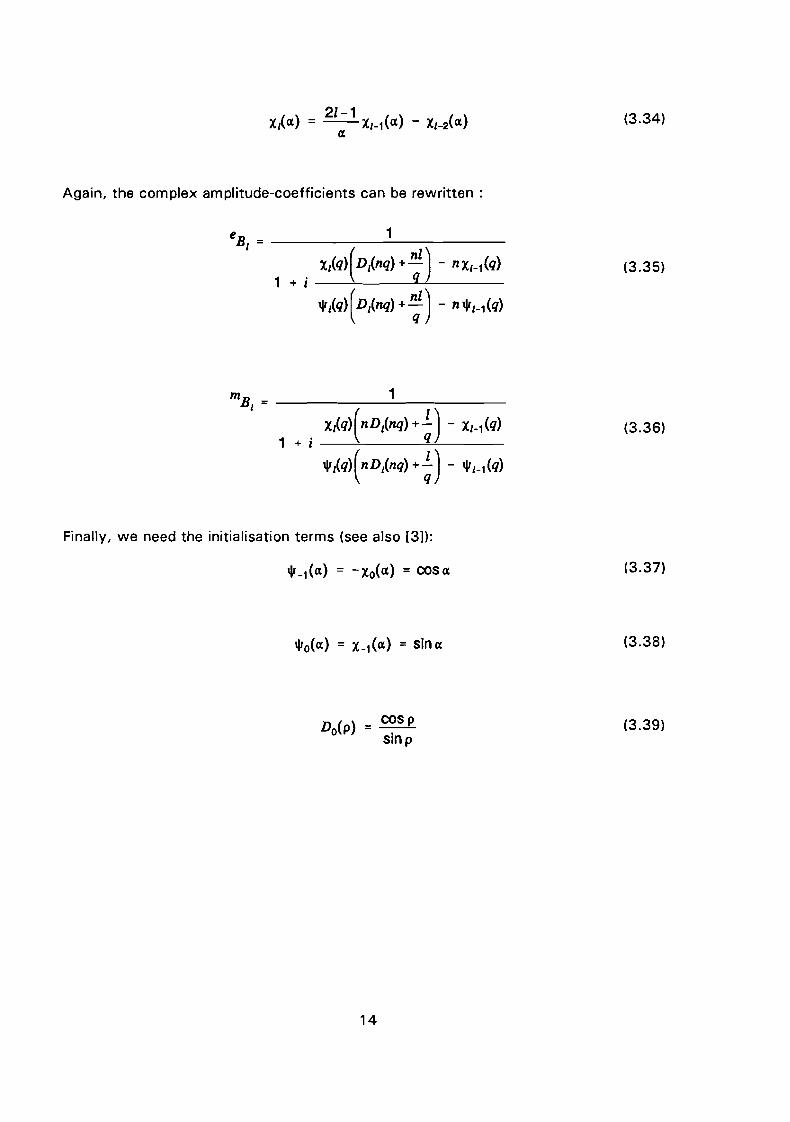
Again, the complex amplitude-coefficients can be rewritten:

eBI = 1 _

1 +i Xl(q) (Dl(nq) +~) -nXI-1(q)

lJrl(q)(Dl(nq) + ~) - nlJrl-1(q)

m 1Bl = ------------

1 + i Xl(q)(nDl(nq) + ~) - XI-1 (q)

lJrl(q)(nDl(nq) + ;) - lJrl-1(q)

Finally, we need the initialisation terms (see also [3]):

lJro(O:) = X_1(0:) = sin 0:

D (p) = ~s po sinp

14

(3.34)

(3.35)

(3.36)

(3.37)

(3.38)

(3.39)

3.5 : Checking computational results.

In programming the Mie-intensity-functions, one should be able to check the various

special functions along the way. This can be done using tables or using approximation­

formulae.

Tables for the associated Legendre-functions can be found in [61. To verify the

calculation of the derivative of these functions, the following numerical formula can be

used (for very small h) :

pf1)(COS6+h) - pf1)(cosa-h)

2h(3.40)

To check the cylindrical Bessel-functions, tables of the original Bessel-functions of order

1+ 1/2 can be used, see [7). Further, for very large values of a (also large compared to

I), we have the approximations:

(3.41 )

(3.42)

For a modulus of a complex p much greater than 1, the following approximation can be

made:

cos(p __iTt )2D1(p):= ----

. ( ITt )sin p--2

(3.43)

The complex coefficients can be checked using a very small value of q. In this case

only the first partial waves can be considered, and we can write:

(3.44)

15

(3.45)

Finally, the Mie-intensity-functions can be verified, comparing them to calculations

Blumer made for n = 1.25'.

table 3.1 : ''''d+ltlln according to Blumer.

lWl q =0.01 q=0.1 q=0.5 q=1 q=2 q=5 q=8

0 5.0E-14 5.0E-8 1.2E-3 2.3E-l 4.3 9.8E+2 7.5E+3

90 2.5E-14 2.5E-8 5.0E-4 3.6E-2 2.5E-l 2.7 7.1

180 5.0E-14 4.9E-8 7.8E-4 1.9E-2 2.0E-2 1.3 0.9

table 3.2 : ''''d+ I tiln according to own calculations.

lWl q=O.Ol q =0.1 q=0.5 q=l q=2 q=5 q=8

0 4.99E-14 5.00E-8 8.30E-4 5.96E-2 4.28 8.36E+2 7.47E+3

90 2.49E-14 2.49E-8 3.73E-4 1.94E-2 2.44E-l 1.52 7.13

180 4.99E-14 4.96E-8 6.70E-4 2.45E-2 2.02E-2 2.98 9.01 E-1

For small and large values of q, the comparison of the two tables turns out right.

However, values near 1 show different values. This is an interesting observation, which

can be explained by the fact that Blumer must have worked with approximation­

formulae, not having a fast computer to perform his calculations.

'Compiled from calculations of H.Blumer, Z.f.Phys., 38(1926),304

16

3.6 : Number of terms in Mie-series.

Having all the necessary relations to calculate Mie-intensity-functions, we only need to

know the number of terms that have to be taken into account. After making a lot of

Mie-scattering calculations, Wiscombe [8] suggests the following for the maximum

number of terms:

'max =

1.01fq + 4q1/3 + 1)

1.01(q + 4.05q '/3 + 2)

1.01fq + 4 q '/3 + 2)

0.02sqs 8

8<q<4200

4200 s q s 20. 000

(3.46)

The calculation of the intensity-functions is done using the programming-language

TURBO-C. Results of calculations will be presented in the next chapter.

17

Chapter 4 : Theoretical results

4.1 : Introduction.

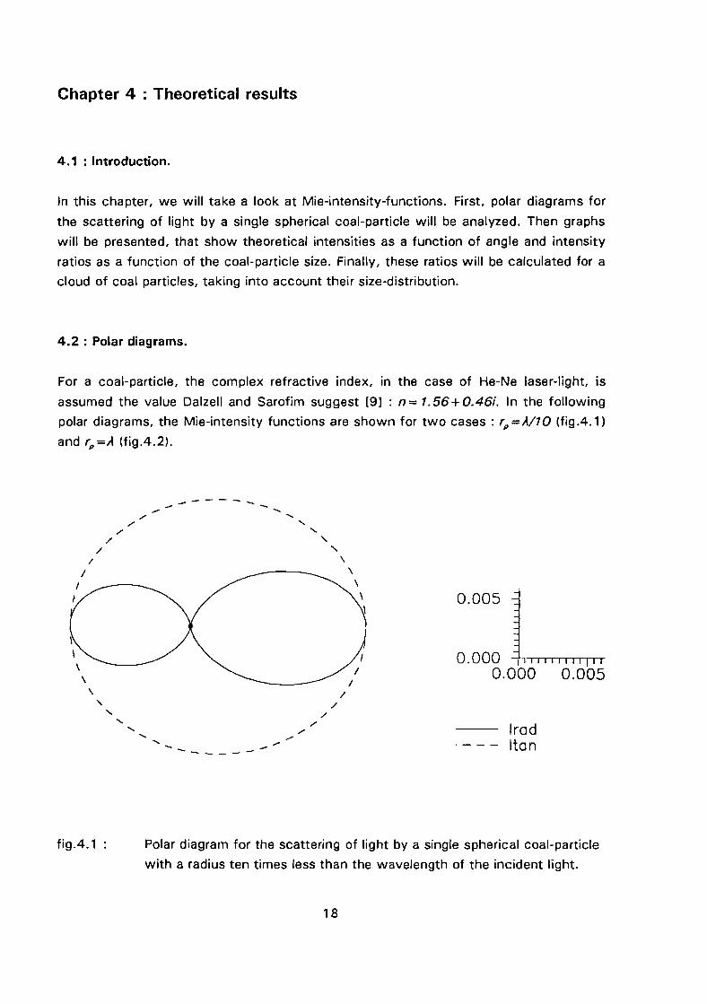
In this chapter, we will take a look at Mie-intensity-functions. First, polar diagrams for

the scattering of light by a single spherical coal-particle will be analyzed. Then graphs

will be presented, that show theoretical intensities as a function of angle and intensity

ratios as a function of the coal-particle size. Finally, these ratios will be calculated for a

cloud of coal particles, taking into account their size-distribution.

4.2 : Polar diagrams.

For a coal-particle, the complex refractive index, in the case of He-Ne laser-light, is

assumed the value Dalzell and Sarofim suggest [9] : n = 1.56+ 0.46;. In the following

polar diagrams, the Mie-intensity functions are shown for two cases: f p =)./10 (fig.4.1)

and f p =). (fig.4.2).

-----...-" "'" "/ .....

/,

/,

I \

/ \

I \

t \ 0.005\

\\ I 0.000 I\ / 0.000 0.005\ /

\ /"- /,

/..... /

" " lrod"' ...-

"' ...- . - -- Itan- - - --

fig.4.1 Polar diagram for the scattering of light by a single spherical coal-particle

with a radius ten times less than the wavelength of the incident light.

18

"""""""" ", " ...,.-

" ..-/ I " ,.-- -

/ "( "/

,.- ..... .."

~

:::: l,,,,,,,,,~\

..... "" \.r ..... 0.00 1.00\.\ .....

" ..... ....-..... -...... 1 ..... ................ ~ ..........

..... ..... ..... Irod..... ..... . - -- Iton

fig.4.2 : Polar diagram for the scattering of light by a single spherical coal-particle

with a radius eaqual to the wavelength of the incIdent light.

Although the tables 3.1 and 3.2 give the sum of the relative intensities for a different

kind of particle, two trends that are also shown in the polar diagrams can be identified.

First, the intensity functions increase with increasing particle-size. Further, as the radius

of the sphere is increased there is no longer symmetry, more light being scattered in

the forward direction than in the opposite direction and we can no longer speak about

Rayleigh-scattering. This phenomenon is known as the Mie-effect. In the case of a

particle very large compared to the wavelength, most of the incident light is reflected,

as follows from geometrical optics.

19

4.3 : Relative intensity as a function of angle of observation.

From now on, we will look at the relative intensity for natural light, being (I"'d+ 'rsn)/2.

This intensity as a function of (J is shown in fig.4.3 for different particle sizes:

10 •

10 5

10

10-1

• • I I • rp - lambda/10...... .... rp lambda

rp - lambda*10n = 1.56 + 0.46i

o 10 20 30 40 50 60 70 80 90

fig.4.3 : Relative intensity as a function of (J for different coal-particle radii.

The theoretical intensities for particle-sizes that will be used in the experiments, are

found in fig.4.4 :

20

10 •

10 •

10 ]

rp = 3E-6 mn = 1.56 + 0.46ilambda = 632.8 nm

10 10

10 •

10 •

rp = 35E-6 mn = 1.56 + 0.46ilambda = 632.8 nm

90BO60 70504030201010 2 TrTT'TTT'"'rTTTTl"'TT'"TTTTT1"'TT'"rTTTT"1r-rrTTT"'TT'"rTTTT"1"'TT'"T"1 10 J -TI-TTTTT'"rTTTT"1"'TT'"TTT"T"T"1I'"T'TTT"1""TT'"TTTT"T"1I'"T'TTT"1""TT'"T"T"T"T"'

o 10 20 30 40 50 60 70 BO 90 0

() ()

fig.4.4 : Relative intensity as a function of () for f p = 3pm and f p = 35pm.

From the previous figures we can conclude that their shapes become more and more

irregular with increasing particle-size. Suppose in our experiment all particles would

have the same radius. say 35 pm. In this case it would be impossible to obtain this

particle-size by measuring intensities at different angles. Even the smaller particles with

a 3pm radius would cause problems. Therefor. the conclusion can be drawn that the

wavelength of the incident light should be more or less in the same order as the radius

of the particles to be measured. Further. the inaccuracy in the angle of observation ()

should be taken as small as possible (this is a matter of experimental set up). Fortuna­

tely. not all particles have the same size and a distribution should be taken into

account. which makes the problem described above less serious. However. we will deal

in the remaining of this chapter and in the experiments only with particles for which

f p = 3pm.

21

4.4 : Intensity ratios.

For the purpose of the experiment, the intensity-ratios for different angles of observa­

tion are important. Scattered light-intensities will be measured at 10, 20 and 30

degrees. Figure 4.5 shows the theoretical ratios for a single spherical coal-particle as a

function of its radius:

1.50.5 1.0rp (1E-6 m)

130/110----- 130/120

lambda - 632.8 E-9 mn = 1.56 + 0.46i

0.0

1 ~""_"""~_"''''... .... ...., ,,,,

\ I, I

\ I\ I

\ I\ ~---, I\ ,,' " I\, , I\ I 'I

\ I "\ I , I

'-' '-'"

10

0.1

100

0.01

fig.4.5 : Intensity ratios for a single spherical coal-particle, using a He-Ne laser.

The graphs stop at f p = 1.5pm, because they become highly irregular for greater

particles. Again it is shown that the size of the particles to be measured compared to

the wavelength of the incident light, is limited by the theory. From fig.4.5 can be

concluded, that the maximum coal particle-size that can be extracted out of such an

experiment, is about 1.2 pm. This problem could be solved using a CO 2-laser, but then

dispersion has to be taken into account. The dependence of wavelength of the incident

light upon the complex refractive index, is described by a model in Appendix 1. The

result of using a CO 2-laser is shown in figure 4.6. Note that the maximum particle size

that can be determined increases as expected.

22

1

10 E-6 m+ 2.16i

0.8

------- --- ---- ---

130/110----- 130/120

lambda ­n = 3.27

.. .. ... ... ... ...""""""""""""""""""

0.0 1.0 2.0rp (1 E-6 m)

3.0

fig.4.6 : Intensity ratios for a single spherical coal-particle, using a CO 2-laser.

In the case of particles having a size-distribution according to (2.13), the ratios of the

intensities after integration as in (2.15) have to be examined as a function of the count

median radius, fpg" For different values of the standard deviation ug , the computational

results are shown in figure 4.7. The integration over all possible particle-sizes (from 0

to 3 Jim) is done using Simpson's rule, with 6400 steps.

The first graph of figure 4.7 (to obtain a clear picture only one intensity ratio is plotted),

shows the result for a standard deviation very close to 1, a case which is almost similar

to that of figure 4.5. In the remaining part of figure 4.7 we see that the graphs become

less irregular with increasing standard deviation. This is caused by the fact, that more

particles with a different radius contribute to the scattering; irregularities in intensities

for single particles are out-averaged by the integration. Greater particle-sizes can now

be determined by this positive effect, because the reversed problem can be solved over

a greater range of (mean) particle-sizes.

23

--

130/120130/110n = 1.56 + 0.46ilambda = 632.8 nmsigma = 1.1

",,\\ ~

\ ","\ ;I..... /

\ I \ ,,'"I I \ /\ I' I\ I \ I

\ I \" ~I\ I\ II ,\ II I__

I I\ ,- ---\ ,,'" I\ I ~

I II I\ I\ I

0.1

.3 0.0 1 ~o-r-r-rT'"T""'T""T-r-T""1:-T"rr-T'"T""'T""T""""""2-r-rr-T'"T""'T""T"""""l

rpg (1 E-6m)1 2rpg (1E-6m)

130/120n = 1.56 + 0.46ilambda = 632.8 nmsigma = 1.001

o

10

100

0.1

----

1 2rpg (1E-6m)

------

130/120130/'10n = 1.56 + OA6ilambda = 632.8 nmsigma = 1.5

1 2rpg (1 E-6m)

'"",.'""I--

II

II

II

II

o

0.1

3

130/120130/110n = 1.56 + 0.46ilambda = 632.8 nmsigma = 1.3

,\\\II\\

II

\ ,.I '"

"I /I I\ I

I II II I

I II I

I "I II I, '"

o

0.1

fig.4.7 : Intensity ratios for coal particles satisfying a log-normal size-distribution.

24

Chapter 5 Setting up the experiment

5.1 : Introduction.

In this chapter the experimental set-up to measure scattered light-intensities will be

outlined. First, the general set-up will be presented. Then, the measurements of

extinction and scattering of light will be discussed. In the design of the measurement

system constraints out of the Mie-theory and rules of geometrical optics have to be

taken into account. Finally, experimental conditions will be outlined.

5.2 : General set-up.

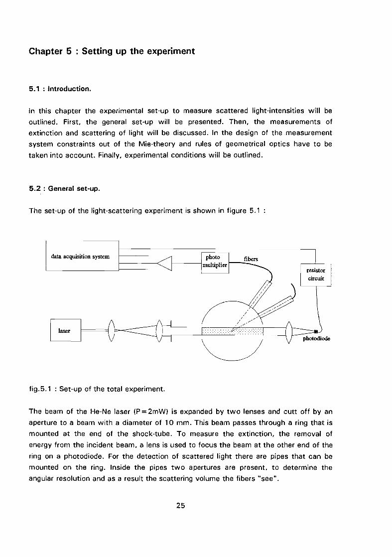
The set-up of the light-scattering experiment is shown in figure 5.1

data acquisition system

fig.5.1 : Set-up of the total experiment.

photomultiplier

fibers

resistorcircuit

The beam of the He-Ne laser IP = 2mW) is expanded by two lenses and cutt off by an

aperture to a beam with a diameter of 10 mm. This beam passes through a ring that is

mounted at the end of the shock-tube. To measure the extinction, the removal of

energy from the incident beam, a lens is used to focus the beam at the other end of the

ring on a photodiode. For the detection of scattered light there are pipes that can be

mounted on the ring. Inside the pipes two apertures are present, to determine the

angular resolution and as a result the scattering volume the fibers "see".

25

In principle one lens and the fiber-head would also have been enough to determine the

angular resolution, but we want to be able to vary this resolution for the different

angles keeping the distance between the apertures constant. This is done at three

different angles, using photomultipliers, because the intensities are too weak for a

photodiode. The output voltages of the photomultipliers are amplified, and together

with the output voltage of the resistor circuit connected to the data aQcuisition system.

This system, to which also a computer is connected, can sample the desired signals

during the time combustion takes place in the shock-tube, about 5 ms.

5.3 : Extinction measurement.

The block in figure 5.1 that is called resistor circuit is in fact a simple electric circuit, as

shown in figure 5.2 :

BPW21

9V+-~

1--------0

820 Q V<:M

'--------------...l-----o

fig.5.2 : Electric circuit for extinction measurement.

With changing intensity of light that falls upon the photodiode, the current changes. As

a result of this, the voltage over the resistor also changes. Because of the properties of

the photodiode, the electric current through the diode (and the resistor) is directly

proportional to the intensity of the beam. If this intensity is diminished by for example

10%, due to the presence of coal particles in the beam, the output voltage Vout is also

diminished by 10%. To measure true extinction, one cannot measure the intensity of

the whole beam that has passed through the ring, because a part of this beam consists

of light scattered to very small angles. Therefor, an aperure has to be used, as shown

in figure 5.3 :

26

•II,I

,'1: i

, I

" ii/i,'

/',I

! --------------------- 220 mm

)4~ d'i__~

fig.5.3 : Limiting the acceptance angle in the extinction measurement.

The diameter do (in mm) of the aperture should be taken small enough, in order to keep

the acceptance angle 8.80 small. Bohren and Huffman [10] suggest the following

criterium:

1.i60 <-2q

From figure 5.3 we obtain for a coal-particle near the surface of the ring:

(5.1 )

do= --

440(5.2)

Combining (5.1) and (5.2), the maximum diameter of the aperture is related to the size

of the particles to be determined. In the experiments an aperture of 2,06 mm is used,

which yields a maximum particle-radius of about 10 Jim. Particles larger than 3 Jim will

not be considered in the experiment.

27

5.4 : Scattering measurement.

To measure scattered light intensities is somewhat more difficult than the extinction

measurement. The instrumentation for the scattering measurement is shown in figure

5.4 :

ring

··53mm··

fig.5.4 : Experimental arrangement for scattering measurement.

On the left side of the drawing, the ring which is mounted to the shock-tube is shown.

The pipes, not shown in this picture, that contain two apertures with diameters d'.1 and

d',2 are attached to this ring. It is important that the inner surface of these pipes is

rough, to avoid reflections that influence the scattering measurement. At the end of

those pipes, the detection of scattered light is done by a bundel of fibers, with a

diameter d'ibers =5 mm. Before the scattered light passes through the two apertures that

determine the acceptance angle 11() and as a result the scattering volume, it passes

through an optical filter with a bandwidth of 10 nm. The windows are constructed such

that dwindow= 15 mm.

There are two possibilities to keep 11() small. First, the distance between the apertures

could be taken large. In this case we would need quite long pipes, that are more

sensitive to oscillations than short ones. Second, the diameters dB. 1 and d,.2 of the

apertures could be taken very small, but the smaller these diameters the more difficult

the construction of the apertures. This means that choises have to be made. First, we

choose 1'= 120 mm and /"= 60 mm. Further, the acceptance angle has to be chosen,

such that dcTo..... 1< dwindow and dCTO.....2 < d'ibers for all angles at which scattering intensities

are to be measured. For scattering angles of 10, 20 and 30 degrees the acceptance

angle 11() is the largest at 30°, and is assumed to be 11()30 =;)0, from which we obtain

dcTO..... 1 =9,061 mm and dCTO.....2 =3,351 mm. Now we can calculate from figure 5.4 the

diameters of the apertures at () =300 : d30• 1 = 6,285 mm and d30,2 = 3,142 mm.

28

Now that for one angle the dimensions of the apertures are known, the scattering

volume is determined. From chapter 2 we know that the apertures at the other angles

must be chosen in such a way that the ratio of No and the square of the distance

between the scattering volume and the detector is the same for every angle. If the

particles in the shock-tube are distributed uniformly, the condition becomes:

(5.3)

In this formula V9 is the scattering volume and f 9 " is the distance between the scatte­

ring volume and the detector. The relevant dimensions can be found in figure 5.5 and

5.6, where the scattering volume is made visible.

fig.5.5 : Instrumental dimensions for scattering measurement.

In this figure the beam diameter dbeam is 10 mm and the inner radius of the ring is

f= 112 mm. Further, all dimensions are taken in mm.

29

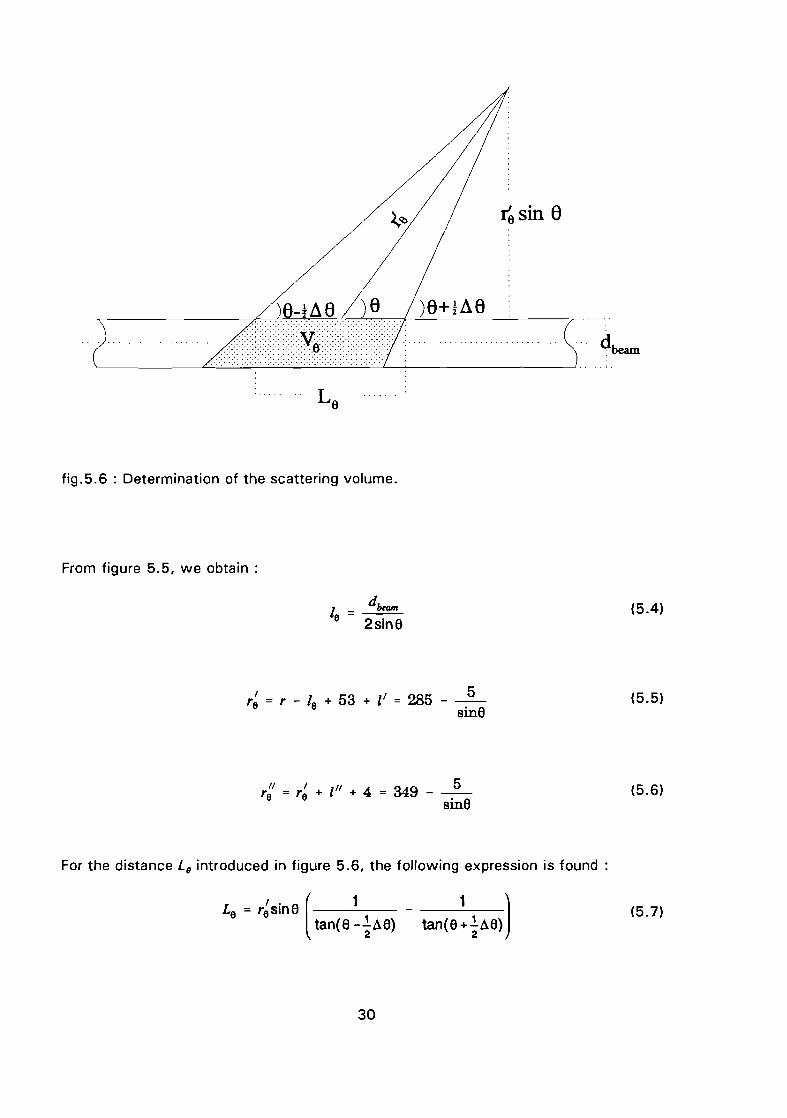
fig.5.6 : Determination of the scattering volume.

From figure 5.5, we obtain:

dbeam

2sin6

~sin e

(5.4)

r~ = r - /e + 53 + [, = 285 5sine

(5.5)

r~' = r~ + [" + 4 = 349 __5_sine

For the distance L9 introduced in figure 5.6, the following expression is found:

L ,. e[ 1 1 1e = reSin - -----tan(e -~~e) tan(6+~~e)

30

(5.6)

(5.7)

If L,< dbeam the scattering volume can be approximated according to :

v. = 1td~ ( 1 - 1 J( I • dlHam1 (5.8)e 4 tan(e -iae) tan(e +iae) re Slne +-2-

Now the value of the constant in (5.3) can be calculated for 8 = 30°, using (5.8),(5.5)

and (5.6) and the acceptance angles for 8= 100 and 8=20° are determined such that

the condition (5.3) is also fulfilled for these angles. The following values are found:

!:::.(),o=0,9300

!:J.()20 = 1,996"

Finally, from figure 5.4 the diameters of the remaining apertures can be determined as:

d ,O, I = 1,947 mm

d10,2 =0,974 mm

d20, I =4,182 mm

d20,2 = 2,091 mm

This completes the experimental set-up.

5.5 : Experimental conditions.

The pressure of the gas in the driver section of the shock-tube is taken 11 bar. In the

test section, the initial pressure of the test gas (02 or N2) is 70 mbar. Just before the

rupture of the membranes between the different sections of the shock-tube, the coal

particles are injected into the test section. In the coal used', the weight percentage of

carbon is 77.7%. The coal-particles have a maximum radius of 3 pm. To avoid multiple

scattering, the concentration of the coal-particles in the scattering volume is limited and

therefore the total weight of the particles to be injected is taken 100 mg.

, European Centre For Coal Specimens SBN, coal sample 236P042.

31

Chapter 6 Experimental results and discussion

6.1 : Introduction.

In the previous chapters both theory and experiment are described. This chapter will

deal with the combination of the two. Results of experiments will be presented and an

effort will be made to verify these results by means of simple calculations. Finally,

suggestions will be given for further experiments, also based on simple calculations.

6.2 : Experimental results.

The first remark that has to be made is one of great implication. With the experimental

set-up as described in the previous chapter, it appears to be impossible to measure

intensities of scattered light during a shock. The reason for this is the fact that the

intensity of light as a result of combustion dominates the scattered light very strongly.

Even if N2 is used as test gas instead of 02' the combustion of O2 inside the coal­

particles causes a light that is much more intense than the scattered light. Furthermore,

this combustion light is "seen" by the fibers in a volume that is much greater than the

scattering volume. To solve this problem, two things have to be done. First, mono­

chromators have to be used instead of the filters, because the bandwidth of the filters

is too big. In this case, a much smaller part of the spectrum of the combustion light is

considered. Second, a stronger laser must be used, to obtain a better ratio between

intensities of scattered light and combustion light. A suggestion to evaluate the laser

power which is necessary for a better experiment is given in the next section.

For the reason described above, measurements are only carried out without combustion

of the coal-particles. After injection of the coal-particles, the output voltages of the

photomultipliers are sampled three times by the data acquisition system (about every

30 seconds) and then averaged. These voltages are related to light intensities, that can

be found after calibration of the photomultipliers using a Tungsten ribbon lamp.

Combining the experimental intensity ratios with theoretical values, some of which are

plotted in figure 4.7, the following table is found for the count median particle-radius

and the expectation of particle-radius:

32

table 6.1 : Results of solving the reversed problem.

Ug rpg [pm] < rp > [pm]

1,1 2,48 2,49

1,2 2,37 2,41

1,3 2,31 2,39

1,4 2,26 2,39

1,5 2,19 2,38

1,6 2,16 2,41

This table shows, that the value of the expectation of particle-radius is more or less

constant (about 2,4 pm), which was to be expected. It is this value that can be

considered to be the effective particle-radius. To obtain the values for this table, only

one intensity ratio is used, 13~/20' because the other one doesn't match with theory.

Probably, the intensity at (J = 10" is not measured correctly. Moreover, different

intensities are measured at 20° and -20°, where one would expect more or less the

same value. Possibly the laser-beam was not exactly in the middle of the shock-tube.

Therefore, one must make sure that the measurements are carried out in an accurate

way. Suggestions for this purpose will be presented in the next section. Note that if

more correct intensity ratios had been used, the effective particle-size, the standard

deviation and the refractive index could have been solved.

6.3 : Discussion.

First the extinction measurement will be discussed, to verify the absence of multiple

scattering. In the experiment, an extinction of 9 % was measured using 100 mg coal.

The rightness of this measurement can be verified using the law of Lambert-Beer:

(6.1)

L is the optical length, in our case two times the inner radius, of the ring and Lp the

free path of the photons. There is no multiple scattering if Lp»L.

33

For the free path the following relation holds:

(6.2)

In this formula N is the concentration of particles in m·3, Q"x,ffp,A,n} the so-called

effective cross section for extinction, which is about 2 times the particles' geometrical

cross section if they are much bigger than the wavelength of the incident light'. Using

formula (6.1) and assuming that all particles in the beam have the same radius, for

example f p =3 pm, we find for the concentration of particles No;::: 8,3'1(fJ m-3 and the

constraint for the absence of multiple scattering is fulfilled.

This concentration can also be determined in another way. It's fair to assume, that the

cloud of coal-particles is spread over a distance of about 2 meters of the shock-tube,

which has of course the same radius as the inner radius of the ring. The volume of the

cloud is in this case:

(6.3)

If the particles are packed together, 1000 kg of coal is often assumed to have a volume

of 1 cubic meter. This means that 100 mg of this coal has a volume of about 10-7 m3•

The volume of a coal-particle with a radius f p =3 pm, can be determined according to :

(6.4)

This means that 100 mg of coal contains about 109 particles, which are spread in the

volume Vc/oud' Using this method, the concentration is found as No;::: 1,3'10'0 m-3•

Of course the two methods described above are not very accurate, because for

example not all particles have the same radius. However, the fact that the concentra­

tions calculated above are of the same order of magnitude, gives us a rough indication

that the extinction measurement is carried out correctly.

'The fact that the effective cross section for extinction is twice the geometricalcross section of the sphere is known as the "extinction-paradox".

34

The power of the laser necessary for measuring scattering during combustion must be

chosen in such a way that scattering intensities are at least equal to the intensity of

emission light. For this purpose, the intensity of scattered light will be related to the

intensity of the laser. From (2.11) we know that for No particles with the same size the

scattered light intensity is found according to :

(6.5)

As an example, we will consider the angle with in theory the smallest scattering

intensity, (] =30°. For this angle the scattering volume is found according to (5.5) and

(5.8) : V30 "" 2350 mm3. From the calculations above, the concentration of particles is

taken 10'0 m-3, which yields for the number of particles in the scattering volume :

No"" 23500. Using (5.6) and substituting theoretical values into (6.5), we find for the

scattering intensity a value which is about 10-5 times the intensity of the laser. The

radius of the original laser beam was first expanded 15 times by the two lenses to a

beam with a diameter of 15 mm, and later cut off by the aperture to a beam of 10 mm

(see fig ure 5.1).

Now the scattered light power can be related to the intensity of the original laser beam

after multiplication by the cross-section of the laser beam:

(6.6)

For the intensity of light (in W1m 2) radiated by a coal-particle during combustion, the

following relation holds:

(6.7)

The constants are :

h=6,63'1O'34 Js, c=3'1OS mis, k= 1,38'10'23 JIK, A = 632,8·1O'9m.

Assumptions have to be made on the other parameters in (6.7). The temperature of the

particle is assumed to be T =3000 K, the emittance ErA) =0,95 and the spectral

resolution of the monochromator ful = 1 A. Substituting these values into (6.7) we

obtain an intensity of light radiated in all directions of about 177 W1m 2•

35

The part of the radiation that is detected by the fibers is dependent upon the solid

angle, which follows from the dimensions of the optical set-up. This angle (10) is

assumed to be the same for all particles in the volume that is seen by the fibers, which

means that a portion of 1/3602 of the emission is detected by the fibers. In fact, this is

a worst-case situation because there are particles that are further away from the fibers

and therefore a smaller solid angle would have to be considered for these particles. The

volume seen by the fibers is in fact a cone with a volume that is about 17,5 times the

scattering volume, which means that in this volume about 17,5,23500 particles are

present. For the power of combustion light that is detected by the fibers, we find:

p . = 561 7·41tr 2 = 635'10-8~mlS • p , [WJ (6.8)

To measure a power of scattered light that is at least equal to the power of combustion

light, the constraint is :

p SJ:at ~ p ~mi3

Finally, using (6.6) and (6.8), the required intensity of the laser is found:

(6.9)

mW

mm 2(6.10)

This means that a stronger laser will be necessary in further experiments. Using a laser

with a beam-radius equal to the beam-radius of the laser used in the experiments, its

power should be at 40 mW instead of 2 mW. The use of monochromators with a

spectral resolution even smaller than 1 A is also possible, so that the laser-intensity can

be smaller than the value in (6.10). Using a laser beam with a smaller diameter would

also diminish the necessity of a more powerful laser, but this would make the measure­

ment less reliable due to a possible displacement of the shock-tube during a shock.

To make the measurements more accurate, the following could be done. First, the

photomultipliers must be calibrated before carrying out the experiments. In this case, it

is possible to measure scattered light intensity at the same angle in several similar

experiments, using different photomultipliers. If the intensities measured by the

different photomultipliers differ too much, it is obvious that they are not calibrated

correctly. After making sure that the calibration was correct, the position of the beam

can be verified, measuring at for example 20° and -20°.

36

If different light intensities are measured, the position of the laser beam has to be

corrected until a satisfactory result is obtained. Of course, one always has to take into

account that the experiments are not perfectly reproducable and that there is always a

certain inaccuracy in the measurements. By doing a lot of experiments, an indication for

this inaccuracy can be found, which can be incorporated in solving the reversed

problem.

37

Chapter 7 . Conclusions

The relative intensity of light scattered by a single spherical particle can be calculated

theoretically as a function of its size and refractive index, the scattering angle and the

wavelength of the incident light. It is also possible to carry out a numerical integration

over more particles of different sizes, taking into account their size distribution.

It is a good thing that in the experiment not all particles have the same size, otherwise

it would not be possible to solve the reversed problem for particles bigger than the

wavelength of the incident light. Taking into account the size distribution of the

particles, it is possible to determine particle-radii of about five times the wavelength of

the incident light.

Scattering of light by a cloud of coal-particles is measured, but this appeared to be

impossible during combustion of the particles. This is due to the weak scattered light

compared to the very intense emission light and the large bandwidth of the filters used.

Therefore, the use of monochromators with a spectral resolution of 1 A in combination

with a laser of at least 40 mW will be necessary in further experiments. Using mono­

chromators with a smaller spectral resolution a laser with less power can be used, but

in any case a stronger laser is recommendable for accurate measurements.

Further, we can conclude that the experiment could have been set up more accurately.

Corrections on the set-up can be made during the experiment if only the photomulti­

pliers are calibrated before and not afterwards.

The com bination of experimental intensity ratios and theoretical values yields an

effective particle-radius which near the assumed geometrical radius of the coal-particles

used.

Finally, the existing computer programs must be expanded with an optimisation routine,

that fits the desired parameters to the experimentally determined intensity-ratios.

38

Chapter 8 References

[1] Born, M. & Wolf, E.

Principles of optics

Pergamom Press, Oxford, 1964.

[2] Hulst, H.C. van de

Light scattering by small particles

Wiley, New York, 1981.

[3] Commissaris, F.A.C.M.

Laser Mie-scattering for shock-tube experiments

Eindhoven University of Technology, Division Electrical Energy Systems,

EUT Faculty of Electrical Engineering, 1991.

[4] Bell, W.W.

Special functions for scientists and engineers

P. van Nostrand Company LTD, London, 1968.

[5] Bohren, C.F.

Recurrence relations for Mie-scattering coefficients

J. Opt. Soc. Am. A, 1987, volA, no.3, p.612-613.

[6] Tables des fonctions de Legendre Associees

Collection Technique Scientifique du CNET, Paris, 1952.

[7] Watson, G.N.

Theory of Bessel-functions

Cambridge University Press, 1966.

39

[8] Wiscombe, W.J.

Improved Mie-scattering algorithms

Applied Optics, 1980, vo1.19, no.9, p.1505-1509.

[9] Dalzell, W.H. & Sarofim, A.F.

Optical constants of soot and their application to heat-flux calculations

Journal of Heat Transfer, 1969, vo1.91, p.100-104.

[10] Bohren, C.F. & Huffman, D

Absorption and scattering of light by small particles

Wiley-Interscience, New York, 1983.

40

Appendix 1 . Dispersion model

To take into account the dependence of the refractive index n = V+iVK upon wave­

length, a dispersion model has been developed by Dalzell and Sarofim [9]. This is done

by fitting constants of the model to experimental results. The final equations concern

propane soot, for which the atomic hydrogen to carbon ratio was 1/4.6. The authors

state that the optical constants for this type of soot don't differ very much from those

of acetylene soot for which H/C = 1/14.7. The latter type is comparable to the coal

used in the experiments, with H/C = 1/1 3.7. The dispersion equations are :

1- Fc e 2/mfo + t 0{wJ -w2)e 2/mfo

g: +w2j-l {wJ _W2)2 + w2g/

(A 1 .1 )

2V2K = Fc g c e2/mfo + t 0w gje

2/mfo

w{g: + w2) j-l {wJ - w2y + w2g/

Explanation of symbols in these formulae:

F number of effective electrons per unit volume

g electron damping constant

w frequency of the radiation

wj natural frequency of the j-th electron

e electronic charge

m electron mass

f o electric permittivity.

(A 1.2)

The subsctript c refers to conduction electrons, j to bound electrons. The constants in

this model are found in table A 1.1 :

41

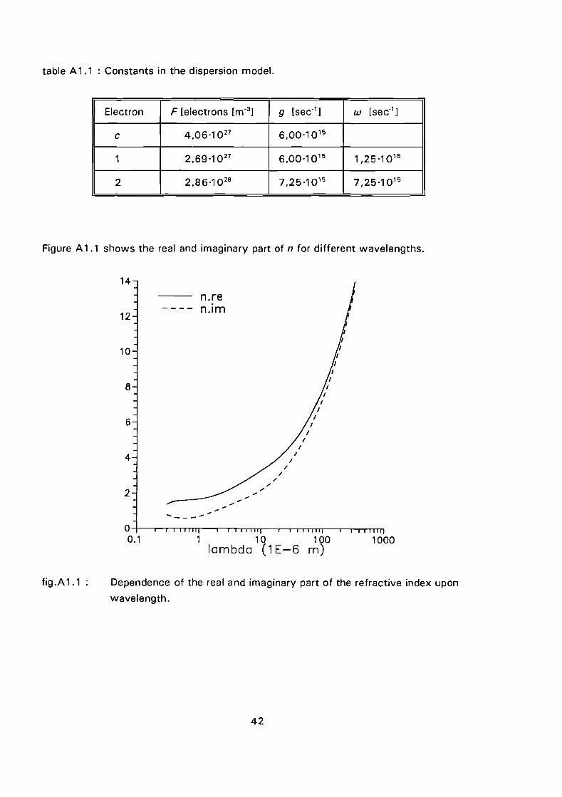
table A 1.1 : Constants in the dispersion model.

Electron F [electrons [m-3] g [sec·1] w [sec·1]

c 4,06'1027 6,00'10 15

1 2,69'1027 6,00'10 15 1,25'1015

2 2,86,1028 7,25'1015 7,25'1015

Figure A 1.1 shows the real and imaginary part of n for different wavelengths.

14

12

n.ren.lm

10

8

6

4

2

,,I

II

II

II

II

II

II

II

//

//.-

""

100010 100lambda (1 E-6 m)

O--t----,r-r-.-rrrrrr--r-l-nrTTTTT"""-r-1......rrrlTT"""-r-l......rrrrn0.1

fig.A 1.1 Dependence of the real and imaginary part of the refractive index upon

wavelength.

42

Samenvatting

In de bestudering van chemische reacties die bepalend zijn voor de verbranding en

vergassing van kooldeeltjes in een schokbuis, is informatie omtrent de grootte van deze

deeltjes gewenst. Een manier om deze deeltjesgrootte te bepalen, is de meting van

intensiteit van laserlicht dat door deze deeltjes wordt verstrooid. Deze intensiteit wordt

onder meer bepaald door de gemiddelde deeltjesgrootte. De theorie die de grootte van

een enkel deeltje relateert aan zijn verstrooiing van Iicht naar verschillende hoeken, is

voor het eerst beschreven door Mie. Het doel van dit werk betreft zowel de implemen­

tatie in computerprogramma's als de experimentele toepassing van deze theorie.

De vergelijkingen van Mie voor de intensiteiten van verstrooid licht bevatten bepaalde

speCiale wiskundige functies, vaak met complexe argumenten. Voor deze functies zijn

geschikte recurrente betrekkingen afgeleid, die snelle berekening van de zg. Mie­

intensiteitsfuncties mogeJijk maken. Verder is een experimentele opstelling geconstru­

eerd om de intensiteit van verstrooid laserlicht te kunnen meten. De dimensies van het

optische gedeelte van de opstelling zijn bepaald volgens regels uit de geometrische

optica, zodaning dat de theorie van Mie toegepast kan worden op het experiment.

De intensiteit van laserlicht verstrooid naar verschillende hoeken is gemeten. Dit bleek

echter niet mogelijk tijdens de verbranding van de kooldeeltjes als gevolg van een sterke

licht-emissie. Na vergelijking van experimentele intensiteitsverhoudingen met berekende

waarden is een effectieve deeltjesradius gevonden, die vergelijkbaar is met de geometri­

sche straal die was aangenomen.

In verdere experimenten zal het gebruik van monochromatoren noodzakelijk zijn. Op die

manier wordt een kleiner gebied in het spectrum van het verbrandingslicht in beschou­

wing genomen. Tevens is een sterkere laser noodzakelijk om de gewenste metingen

mogelijk te maken. De intensiteit van die laser is afhankelijk van de spectrale resolutie

van de monochromatoren die gebruikt wilen worden. Hoe gunstiger de verhouding van

intensiteit van verstrooid licht en verbrandingslicht, hoe nauwkeuriger de meting.

Tenslotte zijn in dit werk nog andere suggesties gegeven met betrekking tot de opbouw

van de experimenten, om ze op een nauwkeuriger manier uit te kunnen voeren.

43