Embed Size (px)
Citation preview
Eindhoven University of Technology
MASTER
Strengthening of reinforced concrete structures with externally bonded carbon fibrereinforcementexperimental research on strengthening of structures in multispan or cantilever situations
Bukman, L.
Award date:2003
Link to publication
DisclaimerThis document contains a student thesis (bachelor's or master's), as authored by a student at Eindhoven University of Technology. Studenttheses are made available in the TU/e repository upon obtaining the required degree. The grade received is not published on the documentas presented in the repository. The required complexity or quality of research of student theses may vary by program, and the requiredminimum study period may vary in duration.
General rightsCopyright and moral rights for the publications made accessible in the public portal are retained by the authors and/or other copyright ownersand it is a condition of accessing publications that users recognise and abide by the legal requirements associated with these rights.
• Users may download and print one copy of any publication from the public portal for the purpose of private study or research. • You may not further distribute the material or use it for any profit-making activity or commercial gain
Experimental research
on strengthening
of structures in
multispan or
cantilever
situations
Strengthening of reinforced concrete structures
with externally bonded carbon fibre reinforcement
Linda BukmanA-2003.1
Appendix
_________________________________________________________________________________________ i Table of Contents
Table of contents Appendix 1 Serviceability limit state 1
Appendix 2 Peeling-off caused at shear cracks 2
Appendix 3 M-κ relation 4
Appendix 4 Material properties single span situation 12
Appendix 5 Critical cross-sections 14
Appendix 6 Mechanisms of failure 17
Appendix 7 Material properties multi span situation 25
Appendix 8 High-speed camera 26
Appendix 9 Data beam 11 to 16 35
Appendix 10 ESPI measurement beam 14 57
_________________________________________________________________________________________ Appendix 1 1 Serviceability limit state
Appendix 1 One of the requirements that have to be met when strengthening a structure with FRP EBR concerns the serviceability limit state. In many of the decisions on the final arrangement of the fibre composite reinforcement, the serviceability limit state appears to be a restricting factor. The following minor calculation makes this statement more conceivable. The stiffness of a concrete structure can be approached by:
25.0 dAEEI ssstructure ⋅≈
with: Es modulus of elasticity of steel reinforcement As cross-section of steel reinforcement d depth of the member When strengthening a structure, material is added to the cross-section. This material has a certain cross-section and stiffness of its own. If FRP EBR is used, the added cross-section and stiffness of the added material can be expressed as Af=αAs and Ef=βEs. The stiffness of the structure may now be approached by:
( )αβ
αβ
+⋅≈
⋅+⋅≈
15.0
5.05.02
22
dAEEIdAEdAEEI
ssstructure
ssssstructure
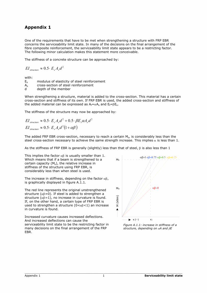
The added FRP EBR cross-section, necessary to reach a certain Ms, is considerably less than the steel cross-section necessary to achieve the same strength increase. This implies α is less than 1. As the stiffness of FRP EBR is generally (slightly) less than that of steel, β is also less than 1 This implies the factor αβ is usually smaller than 1. Which means that if a beam is strengthened to a certain capacity (Ms), the relative increase in stiffness of the structure using FRP EBR, is considerably less than when steel is used. The increase in stiffness, depending on the factor αβ, is graphically displayed in figure A.1.1. The red line represents the original unstrengthened structure (αβ=0). If steel is added to strengthen a structure (αβ=1), no increase in curvature is found. If, on the other hand, a certain type of FRP EBR is used to strengthen a structure (0<αβ<1) an increase in curvature is found. Increased curvature causes increased deflections. And increased deflections can cause the serviceability limit state to be the restricting factor in many decisions on the final arrangement of the FRP EBR.
M (
kNm
)
κ (−)
αβ=0
αβ=0.25αβ=0.5αβ=0.75αβ=1Ms
Mu
κ1
Figure A.1.1: increase in stiffness of a structure, depending on αA and βE
_________________________________________________________________________________________ Appendix 2 2 Peeling-off caused at shear cracks
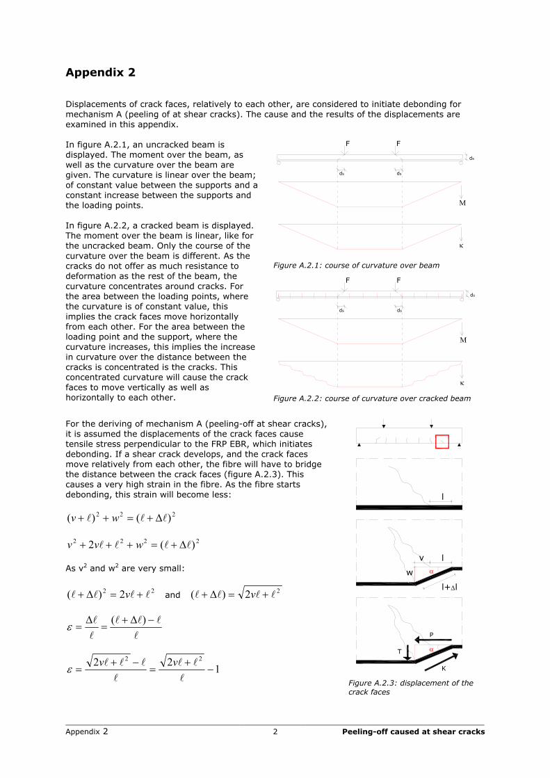
Appendix 2 Displacements of crack faces, relatively to each other, are considered to initiate debonding for mechanism A (peeling of at shear cracks). The cause and the results of the displacements are examined in this appendix.
Μ
F F
κ
dsds
ds
Figure A.2.1: course of curvature over beam
In figure A.2.1, an uncracked beam is displayed. The moment over the beam, as well as the curvature over the beam are given. The curvature is linear over the beam; of constant value between the supports and a constant increase between the supports and the loading points. In figure A.2.2, a cracked beam is displayed. The moment over the beam is linear, like for the uncracked beam. Only the course of the curvature over the beam is different. As the cracks do not offer as much resistance to deformation as the rest of the beam, the curvature concentrates around cracks. For the area between the loading points, where the curvature is of constant value, this implies the crack faces move horizontally from each other. For the area between the loading point and the support, where the curvature increases, this implies the increase in curvature over the distance between the cracks is concentrated is the cracks. This concentrated curvature will cause the crack faces to move vertically as well as horizontally to each other.
FF
ds ds
κ
Μ
ds
Figure A.2.2: course of curvature over cracked beam
For the deriving of mechanism A (peeling-off at shear cracks), it is assumed the displacements of the crack faces cause tensile stress perpendicular to the FRP EBR, which initiates debonding. If a shear crack develops, and the crack faces move relatively from each other, the fibre will have to bridge the distance between the crack faces (figure A.2.3). This causes a very high strain in the fibre. As the fibre starts debonding, this strain will become less:
222 )()( lll ∆+=++ wv
2222 )(2 llll ∆+=+++ wvv
As v2 and w2 are very small:
22 2)( llll +=∆+ v and 22)( llll +=∆+ v
l
lll
l
l −∆+=
∆=
)(ε
122 22
−+
=−+
=l
ll
l
lll vvε
α
P
T
K
α
v l
l+∆l
w
l
Figure A.2.3: displacement of the crack faces
_________________________________________________________________________________________ Appendix 2 3 Peeling-off caused at shear cracks
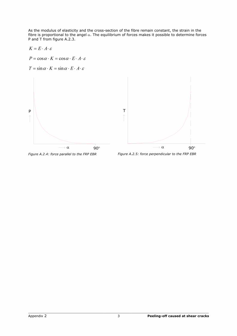
As the modulus of elasticity and the cross-section of the fibre remain constant, the strain in the fibre is proportional to the angel α. The equilibrium of forces makes it possible to determine forces P and T from figure A.2.3.
ε⋅⋅= AEK
εαα ⋅⋅⋅=⋅= AEKP coscos
εαα ⋅⋅⋅=⋅= AEKT sinsin
α
P
90°
Figure A.2.4: force parallel to the FRP EBR
T
α 90°
Figure A.2.5: force perpendicular to the FRP EBR
_________________________________________________________________________________________ Appendix 3 4 M-κ relation
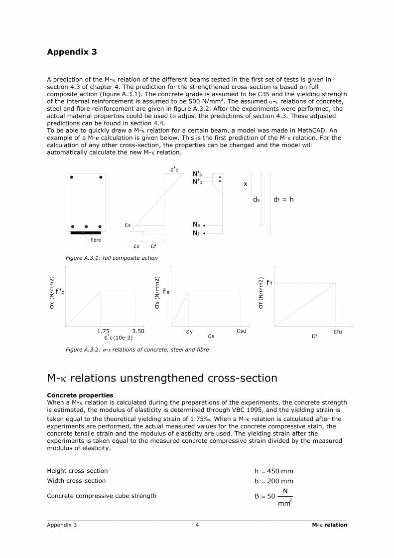
Appendix 3 A prediction of the M-κ relation of the different beams tested in the first set of tests is given in section 4.3 of chapter 4. The prediction for the strengthened cross-section is based on full composite action (figure A.3.1). The concrete grade is assumed to be C35 and the yielding strength of the internal reinforcement is assumed to be 500 N/mm2. The assumed σ-ε relations of concrete, steel and fibre reinforcement are given in figure A.3.2. After the experiments were performed, the actual material properties could be used to adjust the predictions of section 4.3. These adjusted predictions can be found in section 4.4. To be able to quickly draw a M-κ relation for a certain beam, a model was made in MathCAD. An example of a M-κ calculation is given below. This is the first prediction of the M-κ relation. For the calculation of any other cross-section, the properties can be changed and the model will automatically calculate the new M-κ relation.
N'sN'b
Ns
Nf
εf ε0
x
ds df = h
ε'c
εs
fibre
Figure A.3.1: full composite action
1.75 3.50ε'c (10e-3)
σc (
N/m
m2)
f 'c
εs
σs (
N/m
m2)
f s
εy εsu
σf (
N/m
m2)
εf
εfu
f f
Figure A.3.2: σ-ε relations of concrete, steel and fibre
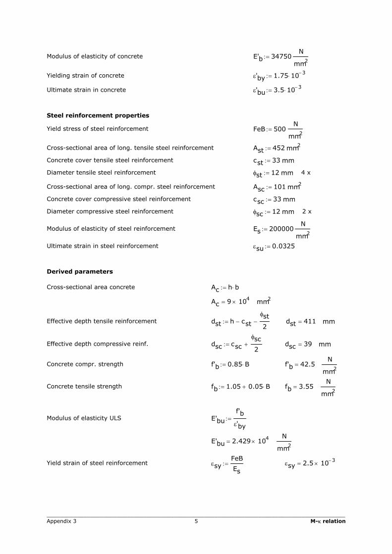
M-κ relations unstrengthened cross-section Concrete properties When a M-κ relation is calculated during the preparations of the experiments, the concrete strength is estimated, the modulus of elasticity is determined through VBC 1995, and the yielding strain is
taken equal to the theoretical yielding strain of 1.75‰. When a M-κ relation is calculated after the experiments are performed, the actual measured values for the concrete compressive stain, the concrete tensile strain and the modulus of elasticity are used. The yielding strain after the experiments is taken equal to the measured concrete compressive strain divided by the measured modulus of elasticity. Height cross-section h 450:= mm
Width cross-section b 200:= mm
Concrete compressive cube strength B 50:=N
mm2
_________________________________________________________________________________________ Appendix 3 5 M-κ relation
Modulus of elasticity of concrete E'b 34750:=N
mm2
Yielding strain of concrete ε'by 1.75 10 3−⋅:=
Ultimate strain in concrete ε'bu 3.5 10 3−⋅:=
Steel reinforcement properties
Yield stress of steel reinforcement FeB 500:=N
mm2
Cross-sectional area of long. tensile steel reinforcement Ast 452:= mm2
Concrete cover tensile steel reinforcement cst 33:= mm
Diameter tensile steel reinforcement φst 12:= mm 4 x
Cross-sectional area of long. compr. steel reinforcement Asc 101:= mm2
Concrete cover compressive steel reinforcement csc 33:= mm
Diameter compressive steel reinforcement φsc 12:= mm 2 x
Modulus of elasticity of steel reinforcement Es 200000:=N
mm2
Ultimate strain in steel reinforcement εsu 0.0325:=
Derived parameters Cross-sectional area concrete Ac h b⋅:=
Ac 9 104×= mm2
Effective depth tensile reinforcement dst h cst−φst
2−:=
dst 411= mm
Effective depth compressive reinf. dsc csc
φsc
2+:=
dsc 39= mm
Concrete compr. strength f'b 0.85 B⋅:=
f'b 42.5=N
mm2
Concrete tensile strength fb 1.05 0.05 B⋅+:=
fb 3.55=N
mm2
Modulus of elasticity ULS E'bu
f'b
ε'by:=
E'bu 2.429 104×=N
mm2
Yield strain of steel reinforcement εsyFeB
Es:=
εsy 2.5 10 3−×=
_________________________________________________________________________________________ Appendix 3 6 M-κ relation
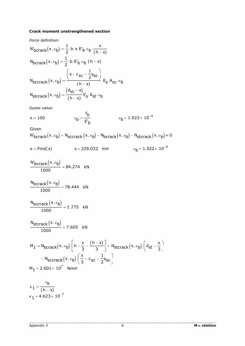
Crack moment unstrengthened section Force definition:
N'bcrack x εb,( ) 1
2b⋅ x⋅ E'b⋅ εb⋅
x
h x−( )⋅:=
Nbcrack x εb,( ) 1
2b⋅ E'b⋅ εb⋅ h x−( )⋅:=
Nsccrack x εb,( )x csc−
1
2φsc−
h x−( )Es⋅ Asc⋅ εb⋅:=
Nstcrack x εb,( )dst x−( )h x−( )
Es Ast⋅ εb⋅:=
Guess value:
x 100:= εb
fb
E'b:=
εb 1.022 10 4−×=
Given
N'bcrack x εb,( ) Nsccrack x εb,( )+ Nbcrack x εb,( )− Nstcrack x εb,( )− 0
x Find x( ):= x 229.032= mm εb 1.022 10 4−×=
N'bcrack x εb,( )
100084.274= kN
Nbcrack x εb,( )
100078.444= kN
Nsccrack x εb,( )
10001.775= kN
Nstcrack x εb,( )
10007.605= kN
M1 Nbcrack x εb,( ) hx
3−
h x−( )
3−
⋅ Nstcrack x εb,( ) dstx
3−
⋅+:=
Nsccrack x εb,( ) x
3csc−
1
2φsc−
⋅−
M1 2.601 107×= Nmm
κ1
εb
h x−( ):=
κ1 4.623 10 7−×=
_________________________________________________________________________________________ Appendix 3 7 M-κ relation
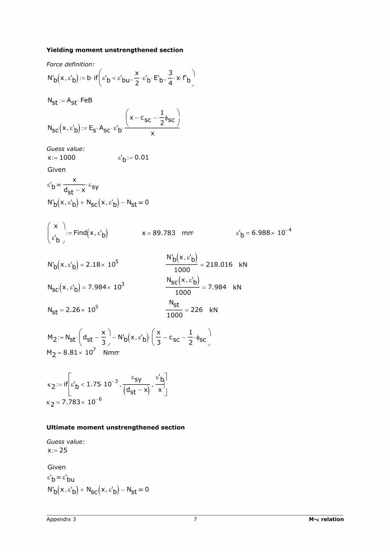
Yielding moment unstrengthened section Force definition:
N'b x ε'b,( ) b if ε'b ε'bu<x
2ε'b⋅ E'b⋅,
3
4x⋅ f'b⋅,
⋅:=
Nst Ast FeB⋅:=
Nsc x ε'b,( ) Es Asc⋅ ε'b⋅
x csc−1
2φsc−
x⋅:=
Guess value: x 1000:= ε'b 0.01:=
Given
ε'bx
dst x−εsy⋅
N'b x ε'b,( ) Nsc x ε'b,( )+ Nst− 0
x
ε'b
Find x ε'b,( ):=
x 89.783= mm ε'b 6.988 10 4−×=
N'b x ε'b,( ) 2.18 105×= N'b x ε'b,( )
1000218.016= kN
Nsc x ε'b,( ) 7.984 103×=
Nsc x ε'b,( )1000
7.984= kN
Nst 2.26 105×=
Nst
1000226= kN
M2 Nst dstx
3−
⋅ N'b x ε'b,( ) x
3csc−
1
2φsc⋅−
⋅−:=
M2 8.81 107×= Nmm
κ2 if ε'b 1.75 10 3−⋅<εsy
dst x−( ),ε'b
x,
:=
κ2 7.783 10 6−×=
Ultimate moment unstrengthened section Guess value: x 25:= Given
ε'b ε'bu
N'b x ε'b,( ) Nsc x ε'b,( )+ Nst− 0
_________________________________________________________________________________________ Appendix 3 8 M-κ relation
x
ε'b
Find x ε'b,( ):=
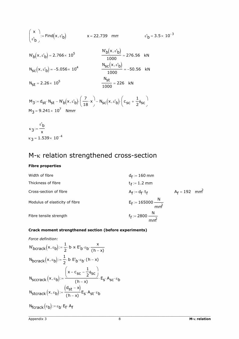
x 22.739= mm ε'b 3.5 10 3−×=
N'b x ε'b,( ) 2.766 105×= N'b x ε'b,( )
1000276.56= kN
Nsc x ε'b,( ) 5.056− 104×=
Nsc x ε'b,( )1000
50.56−= kN
Nst 2.26 105×=
Nst
1000226= kN
M3 dst Nst⋅ N'b x ε'b,( ) 7
18x⋅
⋅− Nsc x ε'b,( ) csc1
2φsc+
⋅−:=
M3 9.241 107×= Nmm
κ3
ε'b
x:=
κ3 1.539 10 4−×=
M-κ relation strengthened cross-section Fibre properties Width of fibre df 160:= mm
Thickness of fibre tf 1.2:= mm
Cross-section of fibre Af df tf⋅:=
Af 192= mm2
Modulus of elasticity of fibre Ef 165000:=N
mm2
Fibre tensile strength ff 2800:=N
mm2
Crack moment strengthened section (before experiments) Force definition:
N'bcrack x εb,( ) 1
2b⋅ x⋅ E'b⋅ εb⋅
x
h x−( )⋅:=
Nbcrack x εb,( ) 1
2b⋅ E'b⋅ εb⋅ h x−( )⋅:=
Nsccrack x εb,( )x csc−
1
2φsc−
h x−( )Es⋅ Asc⋅ εb⋅:=
Nstcrack x εb,( )dst x−( )h x−( )
Es Ast⋅ εb⋅:=
Nfcrack εb( ) εb Ef⋅ Af⋅:=
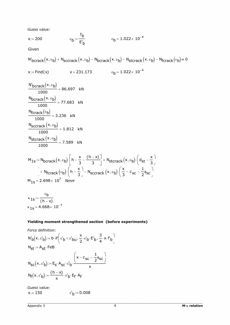
_________________________________________________________________________________________ Appendix 3 9 M-κ relation
Guess value:
x 200:= εb
fb
E'b:=
εb 1.022 10 4−×=
Given N'bcrack x εb,( ) Nsccrack x εb,( )+ Nbcrack x εb,( )− Nstcrack x εb,( )− Nfcrack εb( )− 0
x Find x( ):= x 231.173= εb 1.022 10 4−×=
N'bcrack x εb,( )
100086.697= kN
Nbcrack x εb,( )1000
77.683= kN
Nfcrack εb( )1000
3.236= kN
Nsccrack x εb,( )1000
1.812= kN
Nstcrack x εb,( )1000
7.589= kN
M1s Nbcrack x εb,( ) hx
3−
h x−( )
3−
⋅ Nstcrack x εb,( ) dstx
3−
⋅+:=
Nfcrack εb( ) hx
3−
⋅+ Nsccrack x εb,( ) x
3csc−
1
2φsc−
⋅−
M1s 2.698 107×= Nmm
κ1s
εb
h x−( ):=
κ1s 4.668 10 7−×=
Yielding moment strengthened section (before experiments) Force definition:
N'b x ε'b,( ) b if ε'b ε'bu<x
2ε'b⋅ E'b⋅,
3
4x⋅ f'b⋅,
⋅:=
Nst Ast FeB⋅:=
Nsc x ε'b,( ) Es Asc⋅ ε'b⋅
x csc−1
2φsc−
x⋅:=
Nf x ε'b,( ) h x−( )
xε'b⋅ Ef⋅ Af⋅:=
Guess value: x 150:= ε'b 0.008:=
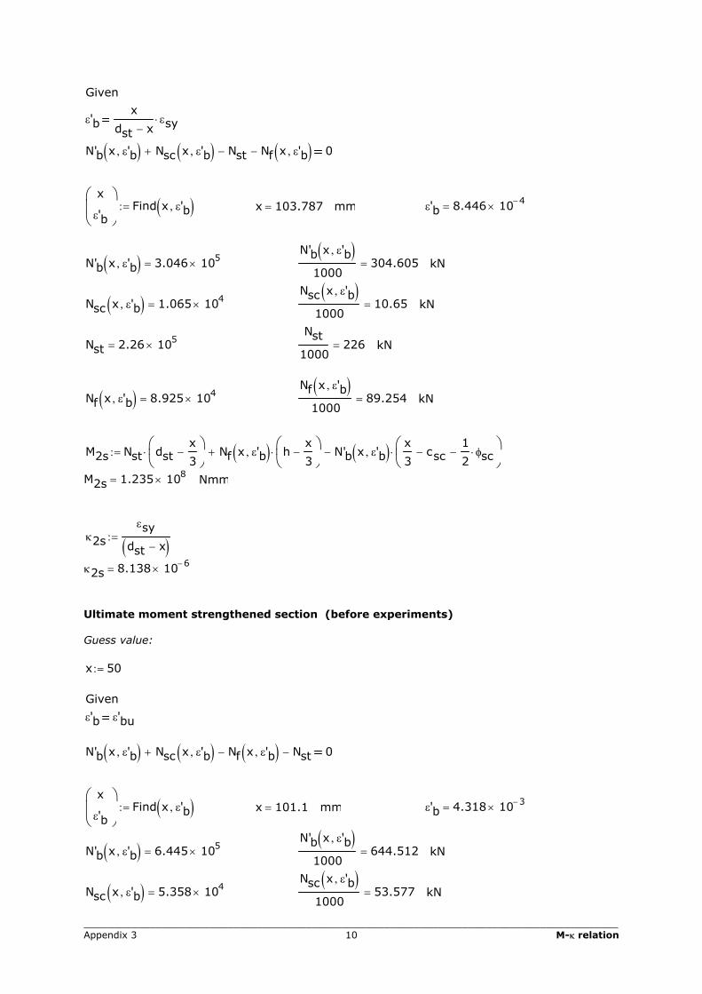
_________________________________________________________________________________________ Appendix 3 10 M-κ relation
Given
ε'bx
dst x−εsy⋅
N'b x ε'b,( ) Nsc x ε'b,( )+ Nst− Nf x ε'b,( )− 0
x
ε'b
Find x ε'b,( ):= x 103.787= mm ε'b 8.446 10 4−×=
N'b x ε'b,( ) 3.046 105×=
N'b x ε'b,( )1000
304.605= kN
Nsc x ε'b,( ) 1.065 104×=
Nsc x ε'b,( )1000
10.65= kN
Nst 2.26 105×=
Nst
1000226= kN
Nf x ε'b,( ) 8.925 104×=
Nf x ε'b,( )1000
89.254= kN
M2s Nst dstx
3−
⋅ Nf x ε'b,( ) hx
3−
⋅+ N'b x ε'b,( ) x
3csc−
1
2φsc⋅−
⋅−:=
M2s 1.235 108×= Nmm
κ2s
εsy
dst x−( ):=
κ2s 8.138 10 6−×=
Ultimate moment strengthened section (before experiments) Guess value: x 50:= Given
ε'b ε'bu
N'b x ε'b,( ) Nsc x ε'b,( )+ Nf x ε'b,( )− Nst− 0
x
ε'b
Find x ε'b,( ):= x 101.1= mm ε'b 4.318 10 3−×=
N'b x ε'b,( ) 6.445 105×= N'b x ε'b,( )
1000644.512= kN
Nsc x ε'b,( ) 5.358 104×=
Nsc x ε'b,( )1000
53.577= kN
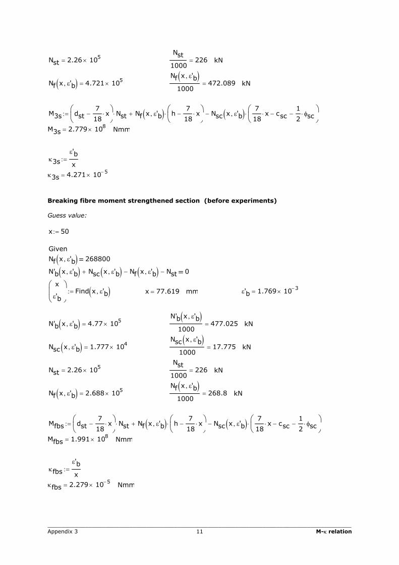
_________________________________________________________________________________________ Appendix 3 11 M-κ relation
Nst 2.26 105×=
Nst
1000226= kN
Nf x ε'b,( ) 4.721 105×=
Nf x ε'b,( )1000
472.089= kN
M3s dst7
18x⋅−
Nst⋅ Nf x ε'b,( ) h7
18x⋅−
⋅+ Nsc x ε'b,( ) 7
18x⋅ csc−
1
2φsc⋅−
⋅−:=
M3s 2.779 108×= Nmm
κ3s
ε'b
x:=
κ3s 4.271 10 5−×=
Breaking fibre moment strengthened section (before experiments) Guess value: x 50:= Given
Nf x ε'b,( ) 268800
N'b x ε'b,( ) Nsc x ε'b,( )+ Nf x ε'b,( )− Nst− 0
x
ε'b
Find x ε'b,( ):=
x 77.619= mm ε'b 1.769 10 3−×=
N'b x ε'b,( ) 4.77 105×=
N'b x ε'b,( )1000
477.025= kN
Nsc x ε'b,( ) 1.777 104×=
Nsc x ε'b,( )1000
17.775= kN
Nst 2.26 105×=
Nst
1000226= kN
Nf x ε'b,( ) 2.688 105×=
Nf x ε'b,( )1000
268.8= kN
Mfbs dst7
18x⋅−
Nst⋅ Nf x ε'b,( ) h7
18x⋅−
⋅+ Nsc x ε'b,( ) 7
18x⋅ csc−
1
2φsc⋅−
⋅−:=
Mfbs 1.991 108×= Nmm
κfbs
ε'b
x:=
κfbs 2.279 10 5−×= Nmm
_________________________________________________________________________________________ Appendix 4 12 Material properties single span situation
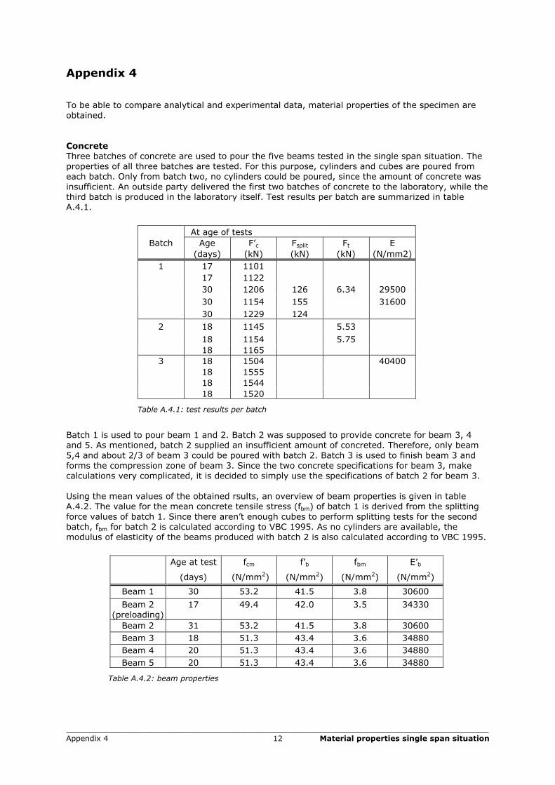
Appendix 4 To be able to compare analytical and experimental data, material properties of the specimen are obtained. Concrete Three batches of concrete are used to pour the five beams tested in the single span situation. The properties of all three batches are tested. For this purpose, cylinders and cubes are poured from each batch. Only from batch two, no cylinders could be poured, since the amount of concrete was insufficient. An outside party delivered the first two batches of concrete to the laboratory, while the third batch is produced in the laboratory itself. Test results per batch are summarized in table A.4.1.
At age of tests
Batch Age F’c Fsplit Ft E (days) (kN) (kN) (kN) (N/mm2) 1 17 1101 17 1122 30 1206 126 6.34 29500 30 1154 155 31600 30 1229 124 2 18 1145 5.53 18 1154 5.75 18 1165 3 18 1504 40400 18 1555 18 1544 18 1520
Table A.4.1: test results per batch Batch 1 is used to pour beam 1 and 2. Batch 2 was supposed to provide concrete for beam 3, 4 and 5. As mentioned, batch 2 supplied an insufficient amount of concreted. Therefore, only beam 5,4 and about 2/3 of beam 3 could be poured with batch 2. Batch 3 is used to finish beam 3 and forms the compression zone of beam 3. Since the two concrete specifications for beam 3, make calculations very complicated, it is decided to simply use the specifications of batch 2 for beam 3. Using the mean values of the obtained rsults, an overview of beam properties is given in table A.4.2. The value for the mean concrete tensile stress (fbm) of batch 1 is derived from the splitting force values of batch 1. Since there aren’t enough cubes to perform splitting tests for the second batch, fbm for batch 2 is calculated according to VBC 1995. As no cylinders are available, the modulus of elasticity of the beams produced with batch 2 is also calculated according to VBC 1995.
Age at test fcm f’b fbm E’b
(days) (N/mm2) (N/mm2) (N/mm2) (N/mm2)
Beam 1 30 53.2 41.5 3.8 30600
Beam 2 (preloading)
17 49.4 42.0 3.5 34330
Beam 2 31 53.2 41.5 3.8 30600 Beam 3 18 51.3 43.4 3.6 34880 Beam 4 20 51.3 43.4 3.6 34880 Beam 5 20 51.3 43.4 3.6 34880
Table A.4.2: beam properties
_________________________________________________________________________________________ Appendix 4 13 Material properties single span situation
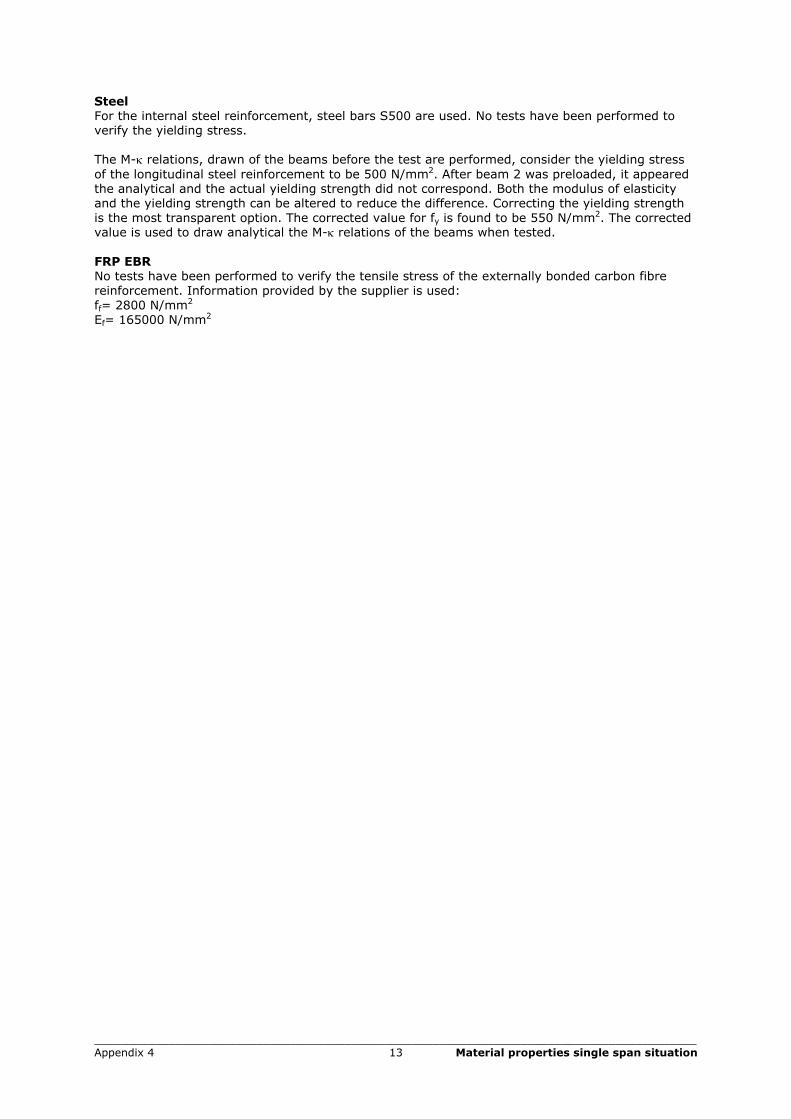
Steel For the internal steel reinforcement, steel bars S500 are used. No tests have been performed to verify the yielding stress. The M-κ relations, drawn of the beams before the test are performed, consider the yielding stress of the longitudinal steel reinforcement to be 500 N/mm2. After beam 2 was preloaded, it appeared the analytical and the actual yielding strength did not correspond. Both the modulus of elasticity and the yielding strength can be altered to reduce the difference. Correcting the yielding strength is the most transparent option. The corrected value for fy is found to be 550 N/mm2. The corrected value is used to draw analytical the M-κ relations of the beams when tested. FRP EBR No tests have been performed to verify the tensile stress of the externally bonded carbon fibre reinforcement. Information provided by the supplier is used: ff= 2800 N/mm2 Ef= 165000 N/mm2

_________________________________________________________________________________________ Appendix 5 14 Critical cross-sections
Appendix 5 To be able to apply the models that describe the mechanisms of failure, a critical section has to be agreed on. In this critical cross-section, the acting forces will be compared to the resisting forces. Since all models were derived from a single span situation, the critical cross-sections in single span structures are derived with the models. A translation to the critical sections in a multi span situation has to be made. Mechanism A; peeling-off caused at shear cracks This model describes a mechanism of failure caused by high shear forces. The shear force in the area in which the FRB EBR is present is therefore restricted to Vodu. This implies the cross-section with maximum shear force is the critical cross-section. In single span situations, this section is situated at the end of the FRP EBR. The actual moment in this section of the beam can be determined from the shifted moment line. According to CUR 91, the critical shear force (Vdmax) is located at distance ds from the end of the FRP EBR (figure A.5.1).
Vd
M
ds
Vdmax
As
Af
ds h
shifted moment
Figure A.5.1: critical section in single span situation
In CUR 91, the translation to a multi span situation has been made. It is assumed all loads to a distance ds from the support are directly passed on to the support. In this case, the critical cross-section in a multi span situation is located at a distance ds from the support. According to CUR 91, this is where Vdmax is located (figure A.5.2). However, if the actual moment has to be determined from the shifted moment line, the actual shear force at a distance ds from the support is located in the section at the edge of the support (Vdmax?).
M
Vd
h
Af
As ds
Vdmax
ds
shifted moment
Vdmax?
Figure A.5.2: critical section at support in multi span situation
_________________________________________________________________________________________ Appendix 5 15 Critical cross-sections
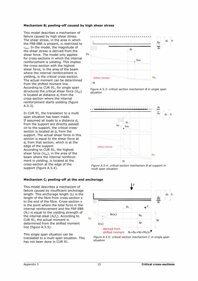
Mechanism B; peeling-off caused by high shear stress This model describes a mechanism of failure caused by high shear stress. The shear stress, in the area in which the FRB EBR is present, is restricted to τosu. In the model, the magnitude of the shear stress is derived from the shear force. The model only applies for cross-sections in which the internal reinforcement is yielding. This implies the cross-section with the highest shear force, in the area of the beam where the internal reinforcement is yielding, is the critical cross-section. The actual moment can be determined from the shifted moment line. According to CUR 91, for single span structures the critical shear force (Vde) is located at distance ds from the
h
Vd
M
shifted moment
Vde
ds Af
Asds
Me
Figure A.5.3: critical section mechanism B in single span situation
cross-section where the internal reinforcement starts yielding (figure A.5.3). In CUR 91, the translation to a multi span situation has been made. If assumed all loads to a distance ds from the support are directly passed on to the support, the critical cross-section is located at ds from the support. The actual shear force in this section is equal to the shear force at ds from that section, which is at the edge of the support. According to CUR 91, the highest shear force (Vde), in the area of the beam where the internal reinforce-ment is yielding, is located at the cross-section at the edge of the support (figure A.5.4).
VdeVd
M
shifted moment
As
Af
ds h
Me
ds
Figure A.5.4: critical section mechanism B at support in multi span situation
Mechanism C; peeling-off at the end anchorage This model describes a mechanism of failure caused by insufficient anchorage length. This anchorage length (lf) is the length of the fibre from cross-section x to the end of the fibre. Cross-section x is the point where the total force in the internal reinforcement and the FRP EBR (Nr) is equal to the yielding strength of the internal steel (Asfy). According to CUR 91, the actual moment is determined from the shifted moment line (figure A.5.5). This single span situation can be translated to a multi span situation. This has not been done in CUR 91.
F
x
lf(x)
Nf(x)
Nf
Ns
Nr=Ns+Nf=Md/zr
As
Af
ds h
derived from shifted moment
Ny
ds
Nr
Figure A.5.5: critical section mechanism C in single span
situation
_________________________________________________________________________________________ Appendix 5 16 Critical cross-sections
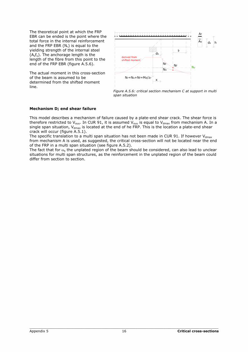
The theoretical point at which the FRP EBR can be ended is the point where the total force in the internal reinforcement and the FRP EBR (Nr) is equal to the yielding strength of the internal steel (Asfy). The anchorage length is the length of the fibre from this point to the end of the FRP EBR (figure A.5.6). The actual moment in this cross-section of the beam is assumed to be determined from the shifted moment line.
Nr=Ns+Nf=Md/zr
derived fromshifted moment
ds
Ny
As
Af
h
lf
x
NfNf
Ns
ds
Figure A.5.6: critical section mechanism C at support in multi span situation
Mechanism D; end shear failure This model describes a mechanism of failure caused by a plate-end shear crack. The shear force is therefore restricted to Vouu. In CUR 91, it is assumed Vouu is equal to Vdmax from mechanism A. In a single span situation, Vdmax is located at the end of he FRP. This is the location a plate-end shear crack will occur (figure A.5.1). The specific translation to a multi span situation has not been made in CUR 91. If however Vdmax from mechanism A is used, as suggested, the critical cross-section will not be located near the end of the FRP in a multi span situation (see figure A.5.2). The fact that for ωs the unplated region of the beam should be considered, can also lead to unclear situations for multi span structures, as the reinforcement in the unplated region of the beam could differ from section to section.
_________________________________________________________________________________________ Appendix 6 17 Mechanisms of failure
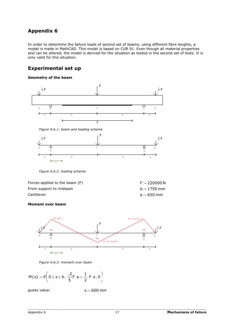
Appendix 6 In order to determine the failure loads of second set of beams, using different fibre lengths, a model is made in MathCAD. This model is based on CUR 91. Even though all material properties and can be altered, the model is derived for the situation as tested in the second set of tests. It is only valid for this situation.
Experimental set up Geometry of the beam
Figure A.6.1: beam and loading scheme
Figure A.6.2: loading scheme
Forces applied to the beam (F) F 220000:= N
From support to midspan b 1750:= mm
Cantilever a 650:= mm Moment over beam
Figure A.6.3: moment over beam
M x( ) if 0 x≤ b≤2−
5F a⋅
1
2F⋅ x⋅+, 0,
:=
guess value: x 600:= mm
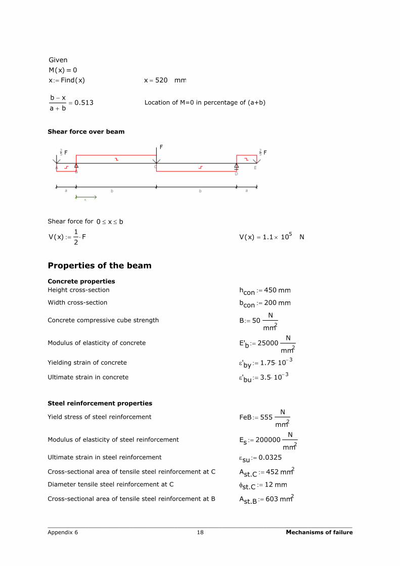
_________________________________________________________________________________________ Appendix 6 18 Mechanisms of failure
Given
M x( ) 0
x Find x( ):= x 520= mm b x−
a b+0.513= Location of M=0 in percentage of (a+b)
Shear force over beam
Shear force for 0 x≤ b≤
V x( )1
2F⋅:=
V x( ) 1.1 105×= N
Properties of the beam Concrete properties Height cross-section hcon 450:= mm
Width cross-section bcon 200:= mm
Concrete compressive cube strength B 50:=N
mm2
Modulus of elasticity of concrete E'b 25000:=N
mm2
Yielding strain of concrete ε'by 1.75 10 3−⋅:=
Ultimate strain in concrete ε'bu 3.5 10 3−⋅:=
Steel reinforcement properties
Yield stress of steel reinforcement FeB 555:=N
mm2
Modulus of elasticity of steel reinforcement Es 200000:=N
mm2
Ultimate strain in steel reinforcement εsu 0.0325:=
Cross-sectional area of tensile steel reinforcement at C Ast.C 452:= mm2
Diameter tensile steel reinforcement at C φst.C 12:= mm
Cross-sectional area of tensile steel reinforcement at B Ast.B 603:= mm2
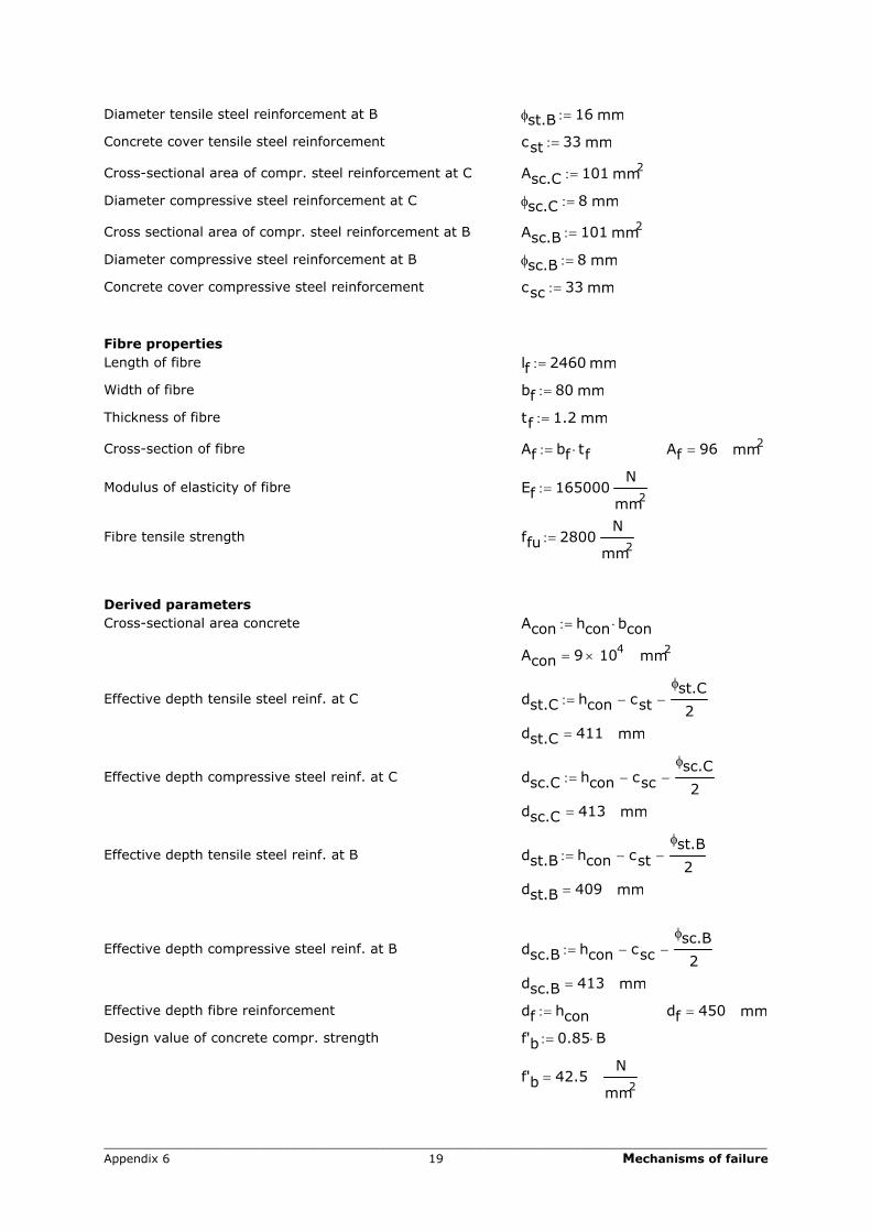
_________________________________________________________________________________________ Appendix 6 19 Mechanisms of failure
Diameter tensile steel reinforcement at B φst.B 16:= mm
Concrete cover tensile steel reinforcement cst 33:= mm
Cross-sectional area of compr. steel reinforcement at C Asc.C 101:= mm2
Diameter compressive steel reinforcement at C φsc.C 8:= mm
Cross sectional area of compr. steel reinforcement at B Asc.B 101:= mm2
Diameter compressive steel reinforcement at B φsc.B 8:= mm
Concrete cover compressive steel reinforcement csc 33:= mm Fibre properties Length of fibre lf 2460:= mm
Width of fibre bf 80:= mm
Thickness of fibre tf 1.2:= mm
Cross-section of fibre Af bf tf⋅:=
Af 96= mm2
Modulus of elasticity of fibre Ef 165000:=N
mm2
Fibre tensile strength ffu 2800:=N
mm2
Derived parameters Cross-sectional area concrete Acon hcon bcon⋅:=
Acon 9 104×= mm2
Effective depth tensile steel reinf. at C dst.C hcon cst−φst.C
2−:=
dst.C 411= mm
Effective depth compressive steel reinf. at C dsc.C hcon csc−φsc.C
2−:=
dsc.C 413= mm
Effective depth tensile steel reinf. at B dst.B hcon cst−φst.B
2−:=
dst.B 409= mm
Effective depth compressive steel reinf. at B dsc.B hcon csc−φsc.B
2−:=
dsc.B 413= mm
Effective depth fibre reinforcement df hcon:=
df 450= mm
Design value of concrete compr. strength f'b 0.85 B⋅:=
f'b 42.5=
N
mm2
_________________________________________________________________________________________ Appendix 6 20 Mechanisms of failure
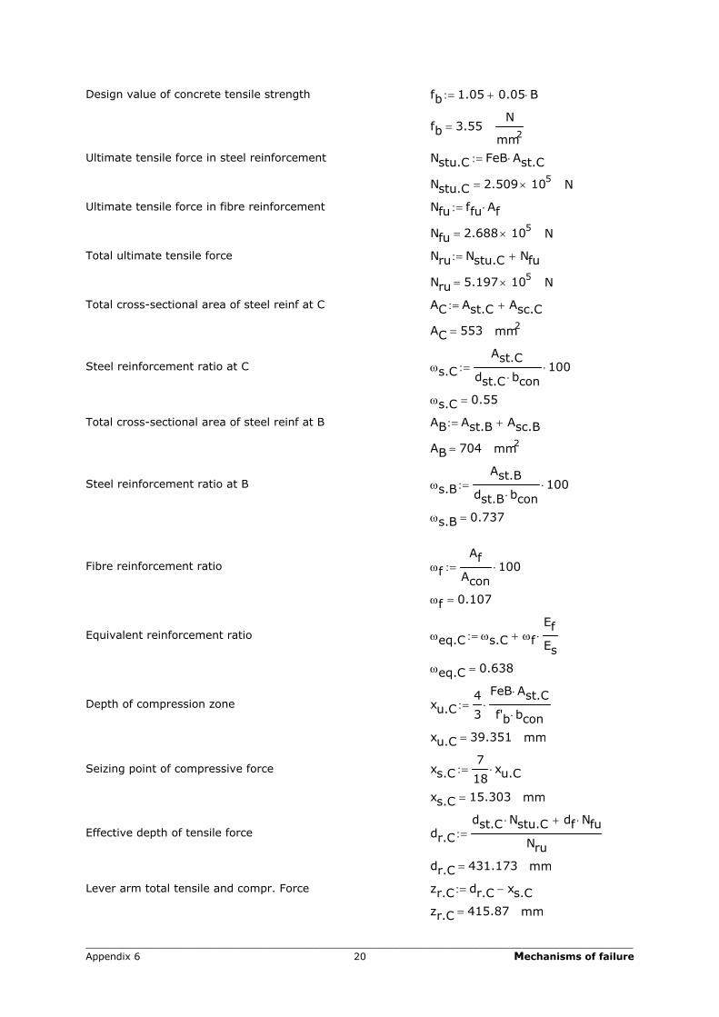
Design value of concrete tensile strength fb 1.05 0.05 B⋅+:=
fb 3.55=
N
mm2
Ultimate tensile force in steel reinforcement Nstu.C FeB Ast.C⋅:=
Nstu.C 2.509 105×= N
Ultimate tensile force in fibre reinforcement Nfu ffu Af⋅:=
Nfu 2.688 105×= N
Total ultimate tensile force Nru Nstu.C Nfu+:=
Nru 5.197 105×= N
Total cross-sectional area of steel reinf at C AC Ast.C Asc.C+:=
AC 553= mm2
Steel reinforcement ratio at C ωs.C
Ast.C
dst.C bcon⋅100⋅:=
ωs.C 0.55=
Total cross-sectional area of steel reinf at B AB Ast.B Asc.B+:=
AB 704= mm2
Steel reinforcement ratio at B
ωs.B
Ast.B
dst.B bcon⋅100⋅:=
ωs.B 0.737=
Fibre reinforcement ratio ωf
Af
Acon100⋅:=
ωf 0.107=
Equivalent reinforcement ratio ωeq.C ωs.C ωf
Ef
Es⋅+:=
ωeq.C 0.638=
Depth of compression zone xu.C4
3
FeB Ast.C⋅
f'b bcon⋅⋅:=
xu.C 39.351= mm
Seizing point of compressive force xs.C7
18xu.C⋅:=
xs.C 15.303= mm
Effective depth of tensile force dr.C
dst.C Nstu.C⋅ df Nfu⋅+
Nru:=
dr.C 431.173= mm
Lever arm total tensile and compr. Force zr.C dr.C xs.C−:=
zr.C 415.87= mm
_________________________________________________________________________________________ Appendix 6 21 Mechanisms of failure
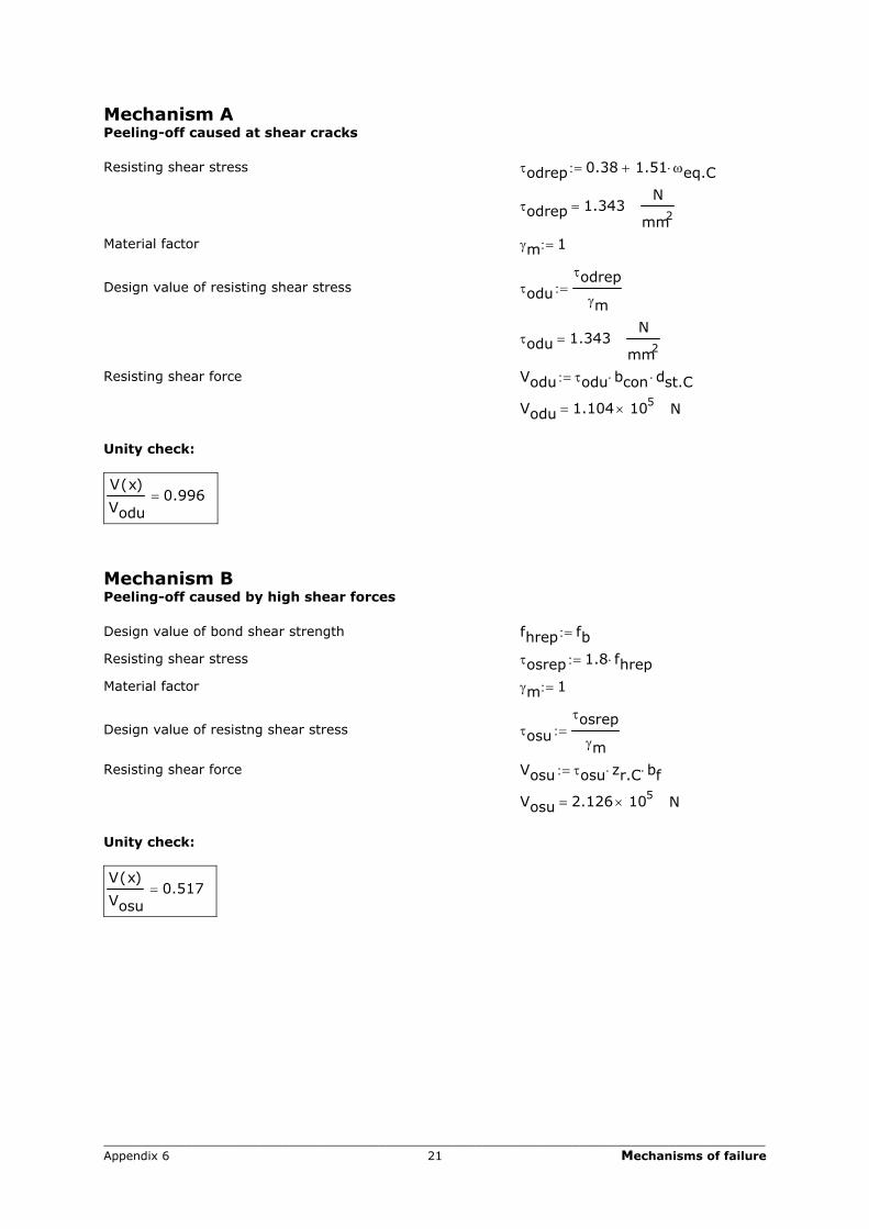
Mechanism A Peeling-off caused at shear cracks Resisting shear stress τodrep 0.38 1.51 ωeq.C⋅+:=
τodrep 1.343=
N
mm2
Material factor γm 1:=
Design value of resisting shear stress τodu
τodrep
γm:=
τodu 1.343=
N
mm2
Resisting shear force Vodu τodu bcon⋅ dst.C⋅:=
Vodu 1.104 105×= N
Unity check:
V x( )
Vodu0.996=
Mechanism B Peeling-off caused by high shear forces Design value of bond shear strength fhrep fb:=
Resisting shear stress τosrep 1.8 fhrep⋅:=
Material factor γm 1:=
Design value of resistng shear stress τosu
τosrep
γm:=
Resisting shear force Vosu τosu zr.C⋅ bf⋅:=
Vosu 2.126 105×= N
Unity check:
V x( )
Vosu0.517=
_________________________________________________________________________________________ Appendix 6 22 Mechanisms of failure
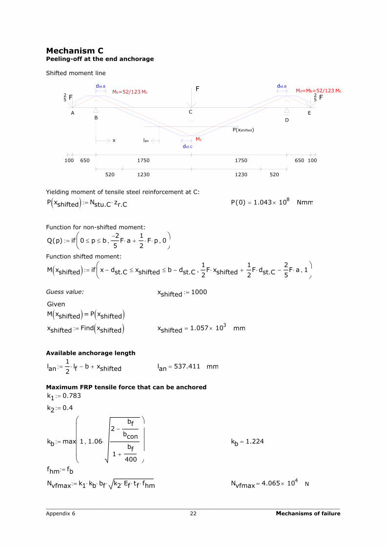
Mechanism C Peeling-off at the end anchorage Shifted moment line
1750650
25 F
BA
Mb=52/123 Mc
6501750
C
F
Mc
D
25 F
E
100 100
520 1230 1230 520
Md=Mb=52/123 Mc
P(xshifted)
dst.C
dst.B dst.B
x lan
Yielding moment of tensile steel reinforcement at C:
P xshifted( ) Nstu.C zr.C⋅:=
P 0( ) 1.043 108×= Nmm
Function for non-shifted moment:
Q p( ) if 0 p≤ b≤
2−
5F a⋅
1
2F⋅ p⋅+, 0,
:=
Function shifted moment:
M xshifted( ) if x dst.C− xshifted≤ b dst.C−≤1
2F xshifted⋅
1
2F dst.C⋅+
2
5F a⋅−, 1,
:=
Guess value: xshifted 1000:=
Given
M xshifted( ) P xshifted( ) xshifted Find xshifted( ):= xshifted 1.057 103×= mm Available anchorage length
lan1
2lf⋅ b− xshifted+:=
lan 537.411= mm
Maximum FRP tensile force that can be anchored k1 0.783:=
k2 0.4:=
kb max 1 1.06
2bf
bcon−
1bf
400+
⋅,
:=
kb 1.224=
fhm fb:=
Nvfmax k1 kb⋅ bf⋅ k2 Ef⋅ tf⋅ fhm⋅⋅:=
Nvfmax 4.065 104×= N
_________________________________________________________________________________________ Appendix 6 23 Mechanisms of failure
Maximum anchorage length
lvfmax
k2 Ef⋅ tf⋅
fhm:= lvfmax 149.365= mm
Force in FRP
Nf xshifted( )M xshifted( )
zr.C 1Ast.C Es⋅
Af Ef⋅+
⋅
:=
Nf xshifted( ) 3.74 104×= N
Required anchorage length
Q lvf( ) lvf( )2 Nvfmax⋅ 2 lvf⋅ Nvfmax⋅ lvfmax⋅− Nf xshifted( ) lvfmax( )2⋅+:=
guess value lvf 100:= mm Given
Q lvf( ) 0
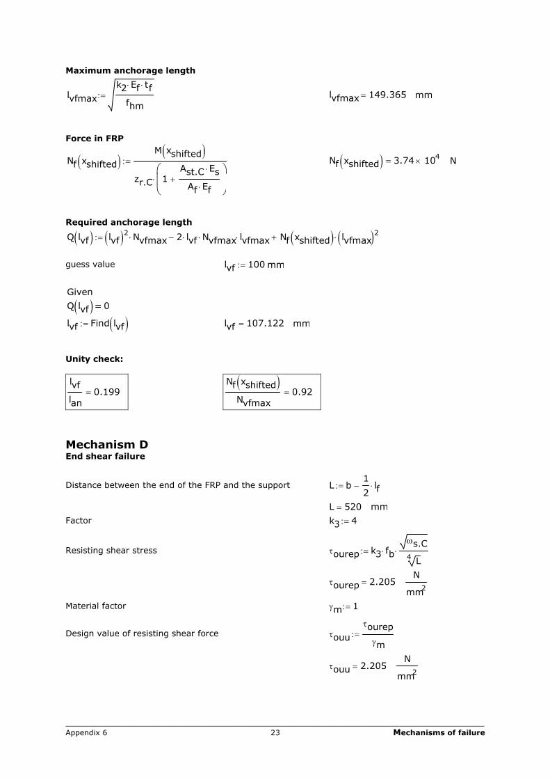
lvf Find lvf( ):= lvf 107.122= mm Unity check:
lvf
lan0.199=
Nf xshifted( )Nvfmax
0.92=
Mechanism D End shear failure
Distance between the end of the FRP and the support L b1
2lf⋅−:=
L 520= mm
Factor k3 4:=
Resisting shear stress τourep k3 fb⋅ωs.C4 L
⋅:=
τourep 2.205=
N
mm2
Material factor γm 1:=
Design value of resisting shear force τouu
τourep
γm:=
τouu 2.205=
N
mm2
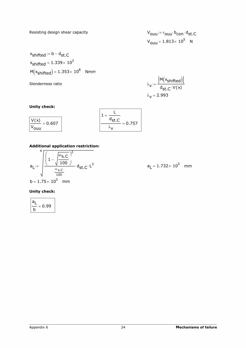
_________________________________________________________________________________________ Appendix 6 24 Mechanisms of failure
Resisting design shear capacity Vouu τouu bcon⋅ dst.C⋅:=
Vouu 1.813 105×= N
xshifted b dst.C−:=
xshifted 1.339 103×=
M xshifted( ) 1.353 108×= Nmm
Slenderness ratio λv
M xshifted( )dst.C V x( )⋅
:=
λv 2.993=
Unity check:
V x( )
Vouu0.607=
1L
dst.C+
λv0.757=
Additional application restriction:
aL
4
1ωs.C
100−
2
ω s.C100
dst.C⋅ L3⋅:= aL 1.732 103×= mm
b 1.75 103×= mm Unity check:
aL
b0.99=
_________________________________________________________________________________________ Appendix 7 25 Material properties multi span situation
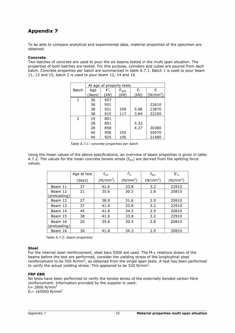
Appendix 7 To be able to compare analytical and experimental data, material properties of the specimen are obtained. Concrete Two batches of concrete are used to pour the six beams tested in the multi span situation. The properties of both batches are tested. For this purpose, cylinders and cubes are poured from each batch. Concrete properties per batch are summarized in table A.7.1. Batch 1 is used to pour beam 11, 13 and 15, batch 2 is used to pour beam 12, 14 and 16.
At age of property tests
Batch Age F’c Fsplit Ft E (days) (kN) (kN) (kN) (N/mm2) 1 36 957 36 951 22610 38 921 109 5.88 23870 38 915 117 3.84 22250 2 19 801 28 891 5.32 28 858 4.27 20380 40 956 105 20570 40 925 100 21480
Table A.7.1: concrete properties per batch Using the mean values of the above specifications, an overview of beam properties is given in table A.7.2. The values for the mean concrete tensile stress (fbm) are derived from the splitting force values.
Age at test fcm f’b fbm E’b
(days) (N/mm2) (N/mm2) (N/mm2) (N/mm2)
Beam 11 37 41.6 33.8 3.2 22910 Beam 12
(preloading) 21 35.6 30.3 2.8 20810
Beam 12 27 38.9 31.6 2.9 20810 Beam 13 37 41.6 33.8 3.2 22910 Beam 14 45 41.8 34.3 2.9 20810 Beam 15 38 41.6 33.8 3.2 22910
Beam 16 (preloading)
20 35.6 30.3 2.8 20810
Beam 16 36 41.8 34.3 2.9 20810
Table A.7.2: beam properties
Steel For the internal steel reinforcement, steel bars S500 are used. The M-κ relations drawn of the beams before the test are performed, consider the yielding stress of the longitudinal steel reinforcement to be 550 N/mm2, as obtained from the single span tests. A test has been performed to verify the actual yielding stress. This appeared to be 520 N/mm2. FRP EBR No tests have been performed to verify the tensile stress of the externally bonded carbon fibre reinforcement. Information provided by the supplier is used: ff= 2800 N/mm2 Ef= 165000 N/mm2
_________________________________________________________________________________________ Appendix 8 26 High-speed camera
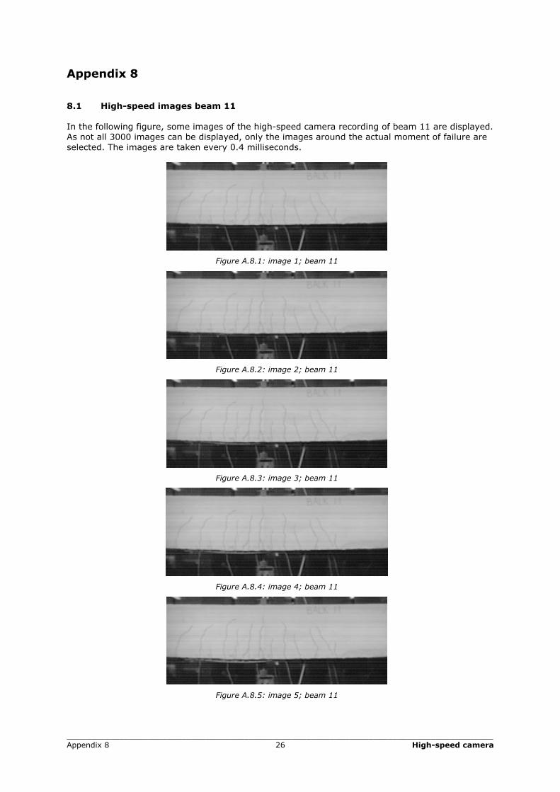
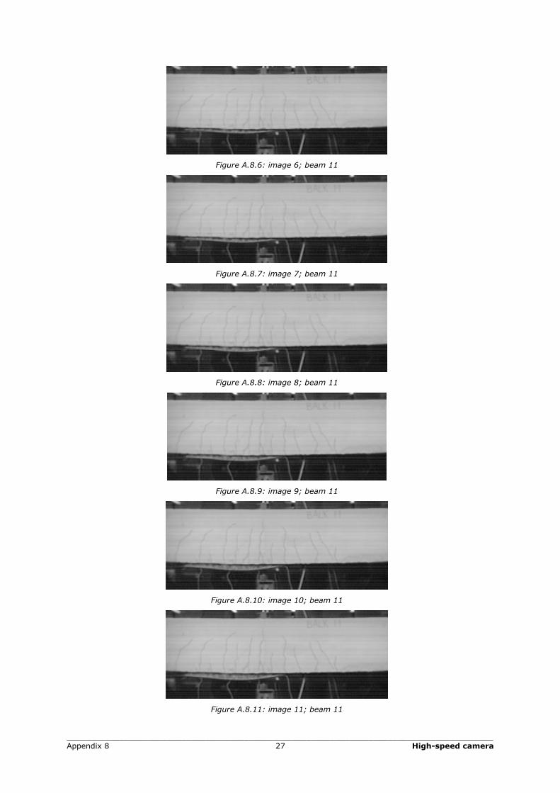
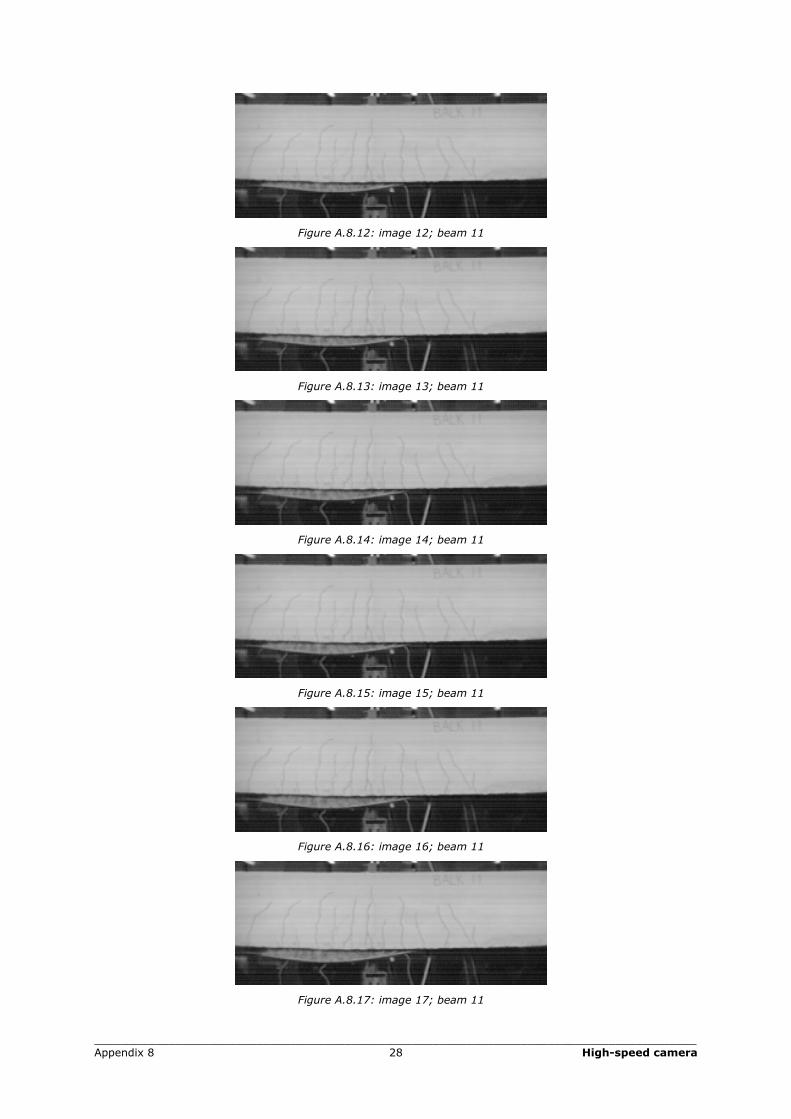
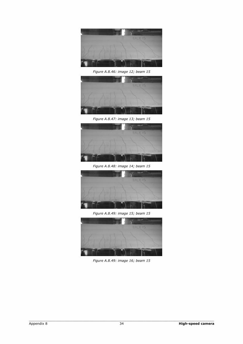
Appendix 8 8.1 High-speed images beam 11 In the following figure, some images of the high-speed camera recording of beam 11 are displayed. As not all 3000 images can be displayed, only the images around the actual moment of failure are selected. The images are taken every 0.4 milliseconds.
Figure A.8.1: image 1; beam 11
Figure A.8.2: image 2; beam 11
Figure A.8.3: image 3; beam 11
Figure A.8.4: image 4; beam 11
Figure A.8.5: image 5; beam 11
_________________________________________________________________________________________ Appendix 8 27 High-speed camera
Figure A.8.6: image 6; beam 11
Figure A.8.7: image 7; beam 11
Figure A.8.8: image 8; beam 11
Figure A.8.9: image 9; beam 11
Figure A.8.10: image 10; beam 11
Figure A.8.11: image 11; beam 11
_________________________________________________________________________________________ Appendix 8 28 High-speed camera
Figure A.8.12: image 12; beam 11
Figure A.8.13: image 13; beam 11
Figure A.8.14: image 14; beam 11
Figure A.8.15: image 15; beam 11
Figure A.8.16: image 16; beam 11
Figure A.8.17: image 17; beam 11
_________________________________________________________________________________________ Appendix 8 29 High-speed camera
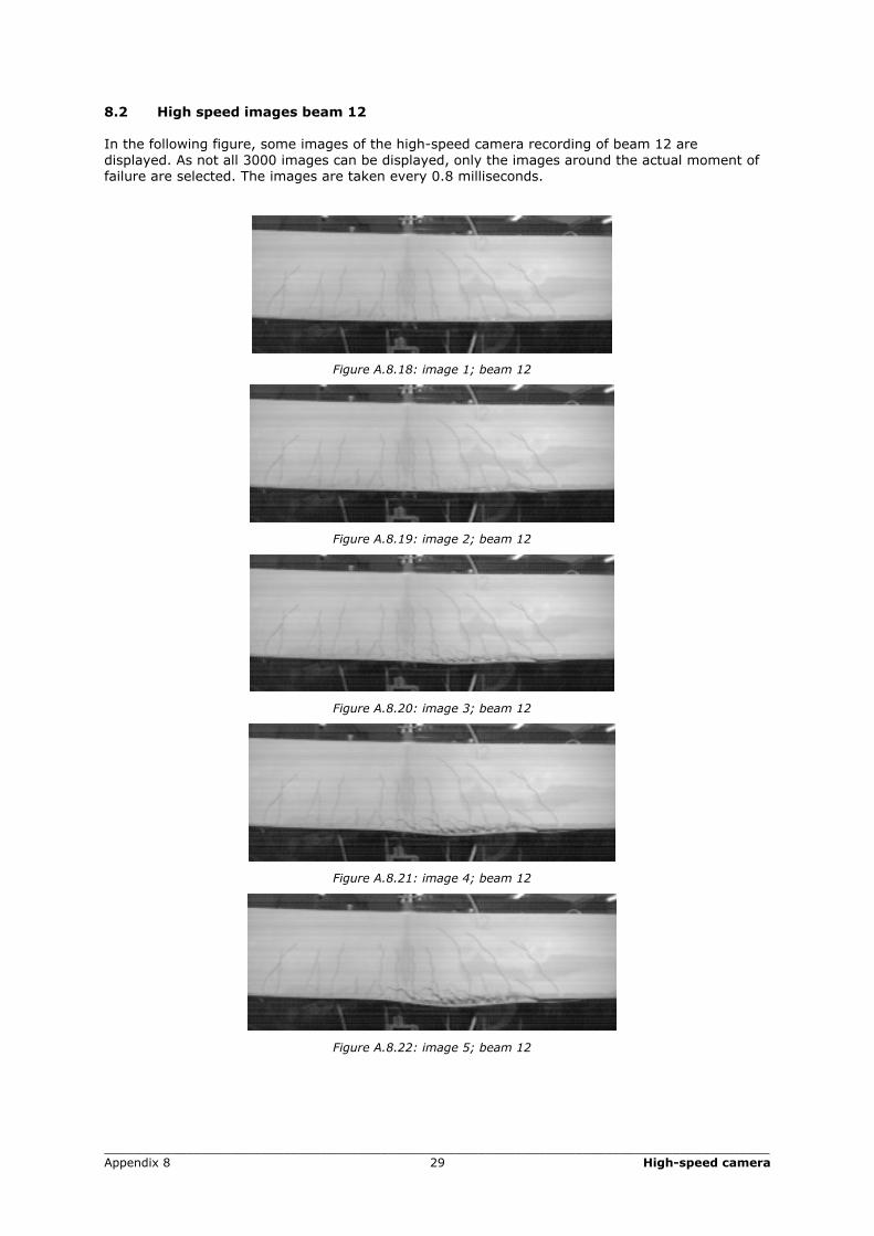
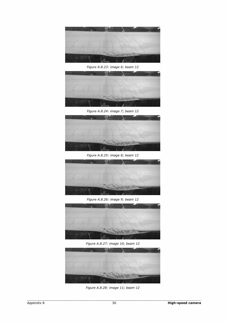
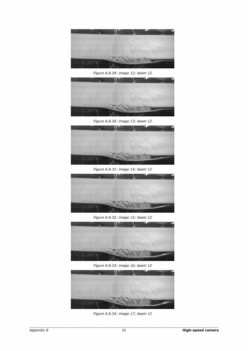
8.2 High speed images beam 12 In the following figure, some images of the high-speed camera recording of beam 12 are displayed. As not all 3000 images can be displayed, only the images around the actual moment of failure are selected. The images are taken every 0.8 milliseconds.
Figure A.8.18: image 1; beam 12
Figure A.8.19: image 2; beam 12
Figure A.8.20: image 3; beam 12
Figure A.8.21: image 4; beam 12
Figure A.8.22: image 5; beam 12
_________________________________________________________________________________________ Appendix 8 30 High-speed camera
Figure A.8.23: image 6; beam 12
Figure A.8.24: image 7; beam 12
Figure A.8.25: image 8; beam 12
Figure A.8.26: image 9; beam 12
Figure A.8.27: image 10; beam 12
Figure A.8.28: image 11; beam 12
_________________________________________________________________________________________ Appendix 8 31 High-speed camera
Figure A.8.29: image 12; beam 12
Figure A.8.30: image 13; beam 12
Figure A.8.31: image 14; beam 12
Figure A.8.32: image 15; beam 12
Figure A.8.33: image 16; beam 12
Figure A.8.34: image 17; beam 12
_________________________________________________________________________________________ Appendix 8 32 High-speed camera
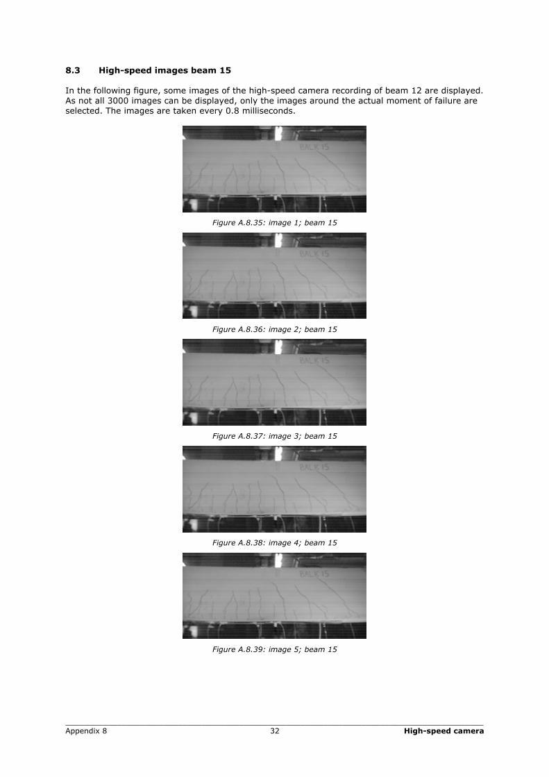
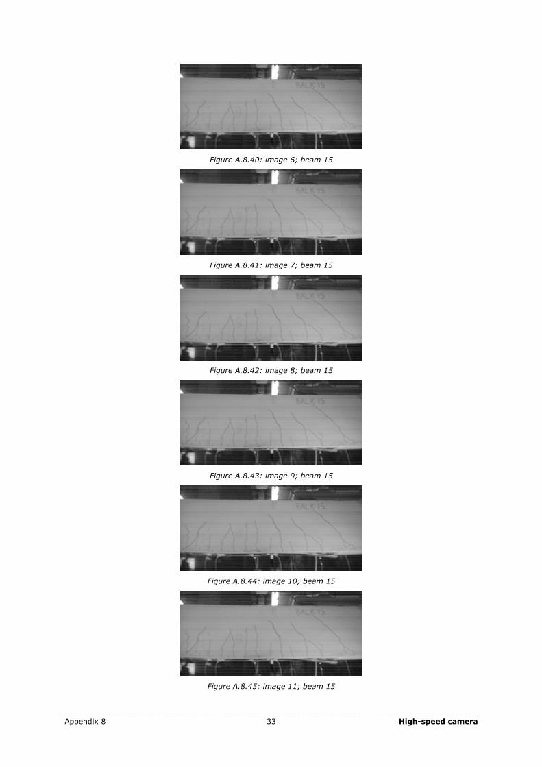
8.3 High-speed images beam 15 In the following figure, some images of the high-speed camera recording of beam 12 are displayed. As not all 3000 images can be displayed, only the images around the actual moment of failure are selected. The images are taken every 0.8 milliseconds.
Figure A.8.35: image 1; beam 15
Figure A.8.36: image 2; beam 15
Figure A.8.37: image 3; beam 15
Figure A.8.38: image 4; beam 15
Figure A.8.39: image 5; beam 15
_________________________________________________________________________________________ Appendix 8 33 High-speed camera
Figure A.8.40: image 6; beam 15
Figure A.8.41: image 7; beam 15
Figure A.8.42: image 8; beam 15
Figure A.8.43: image 9; beam 15
Figure A.8.44: image 10; beam 15
Figure A.8.45: image 11; beam 15
_________________________________________________________________________________________ Appendix 8 34 High-speed camera
Figure A.8.46: image 12; beam 15
Figure A.8.47: image 13; beam 15
Figure A.8.48: image 14; beam 15
Figure A.8.49: image 15; beam 15
Figure A.8.49: image 16; beam 15
_________________________________________________________________________________________ Appendix 9 35 Data beam 11 to 16
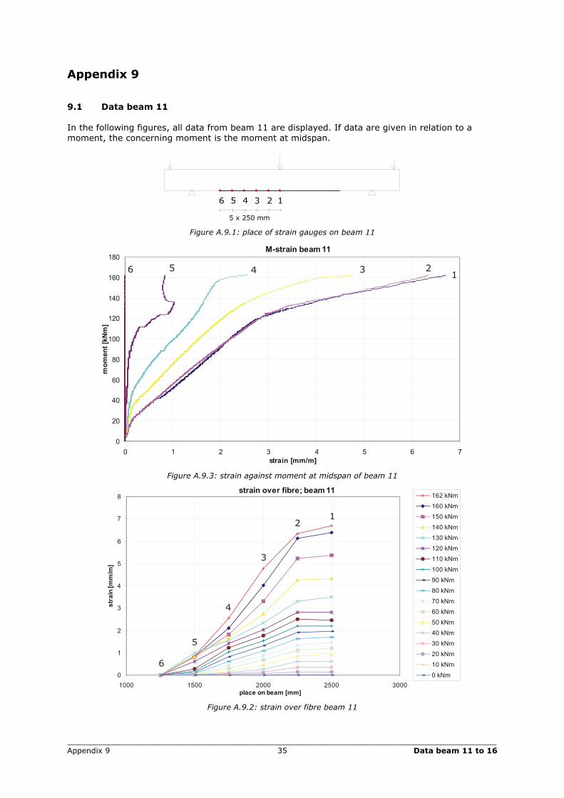
Appendix 9 9.1 Data beam 11 In the following figures, all data from beam 11 are displayed. If data are given in relation to a moment, the concerning moment is the moment at midspan.
6 5 4 3 2 1
5 x 250 mm
Figure A.9.1: place of strain gauges on beam 11
M-strain beam11
0
20
40
60
80
100
120
140
160
180
0 1 2 3 4 5 6 7strain [mm/m]
mom
ent[kNm]
56 4 3 21
Figure A.9.3: strain against moment at midspan of beam 11
strain over fibre; beam11
0
1
2
3
4
5
6
7
8
1000 1500 2000 2500 3000place on beam [mm]
strain[mm/m]
162 kNm
160 kNm
150 kNm140 kNm
130 kNm120 kNm
110 kNm
100 kNm90 kNm
80 kNm
70 kNm60 kNm
50 kNm
40 kNm30 kNm
20 kNm10 kNm
0 kNm
12
3
4
6
Figure A.9.2: strain over fibre beam 11
_________________________________________________________________________________________ Appendix 9 36 Data beam 11 to 16
A B C D E
100 650 1750 1750 650 100
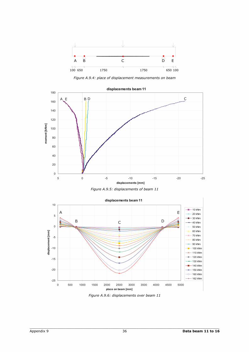
Figure A.9.4: place of displacement measurements on beam
displacements beam11
0
20
40
60
80
100
120
140
160
180
-25-20-15-10-505displacements [mm]
mom
ent[kNm]
A E B CD
Figure A.9.5: displacements of beam 11
displacements beam11
-25
-20
-15
-10
-5
0
5
10
0 500 1000 1500 2000 2500 3000 3500 4000 4500 5000place on beam [mm]
displacement[mm]
10 kNm
20 kNm
30 kNm
40 kNm
50 kNm
60 kNm
70 kNm
80 kNm
90 kNm
100 kNm
110 kNm
120 kNm
130 kNm
140 kNm
150 kNm
160 kNm
162 kNm
A
B C D
E
Figure A.9.6: displacements over beam 11
_________________________________________________________________________________________ Appendix 9 37 Data beam 11 to 16
21
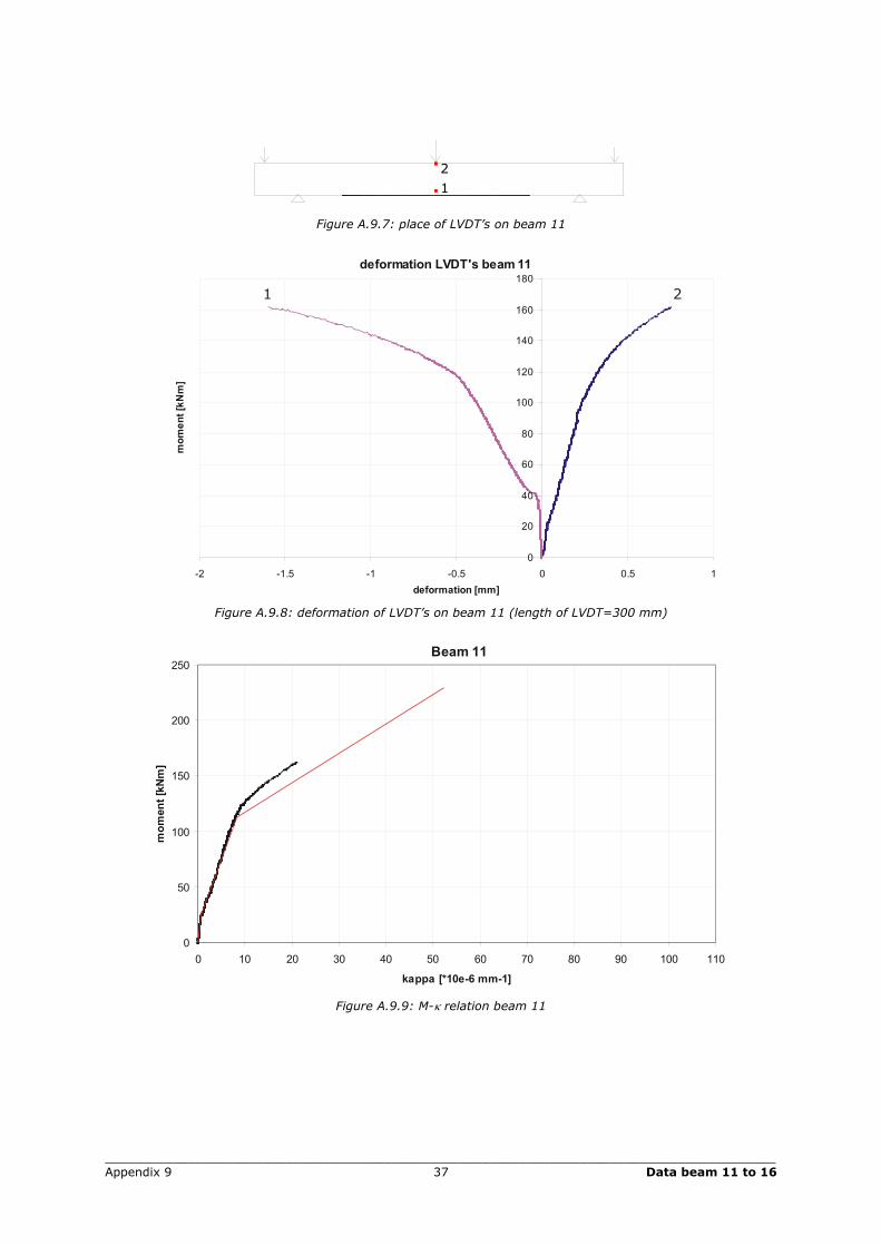
Figure A.9.7: place of LVDT’s on beam 11
deformation LVDT's beam11
0
20
40
60
80
100
120
140
160
180
-2 -1.5 -1 -0.5 0 0.5 1deformation [mm]
mom
ent[kNm]
1 2
Figure A.9.8: deformation of LVDT’s on beam 11 (length of LVDT=300 mm)
Beam 11
0
50
100
150
200
250
0 10 20 30 40 50 60 70 80 90 100 110
kappa [*10e-6 mm-1]
mom
ent[kNm]
Figure A.9.9: M-κ relation beam 11
_________________________________________________________________________________________ Appendix 9 38 Data beam 11 to 16
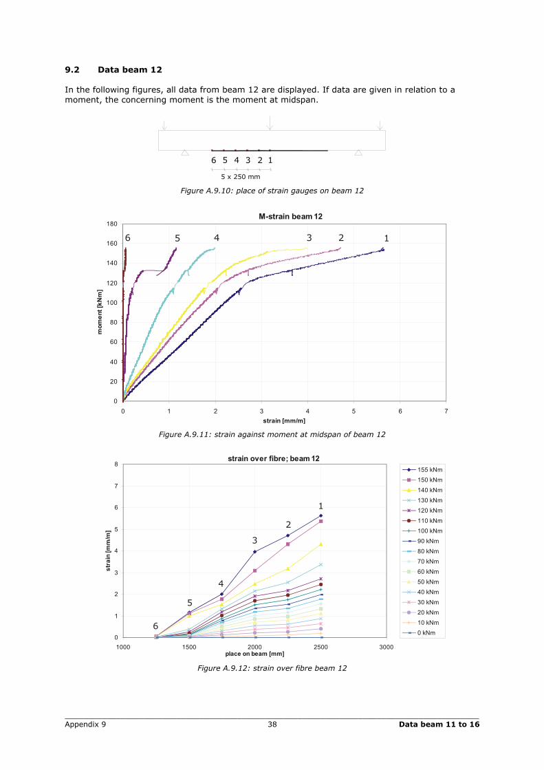
9.2 Data beam 12 In the following figures, all data from beam 12 are displayed. If data are given in relation to a moment, the concerning moment is the moment at midspan.
6 5 4 3 2 1
5 x 250 mm
Figure A.9.10: place of strain gauges on beam 12
M-strain beam12
0
20
40
60
80
100
120
140
160
180
0 1 2 3 4 5 6 7strain [mm/m]
moment[kNm]
123456
Figure A.9.11: strain against moment at midspan of beam 12
strain over fibre; beam12
0
1
2
3
4
5
6
7
8
1000 1500 2000 2500 3000place on beam [mm]
strain[mm/m]
155 kNm150 kNm
140 kNm
130 kNm120 kNm
110 kNm100 kNm
90 kNm
80 kNm70 kNm
60 kNm
50 kNm40 kNm
30 kNm
20 kNm10 kNm
0 kNm
1
2
3
4
5
6
Figure A.9.12: strain over fibre beam 12
_________________________________________________________________________________________ Appendix 9 39 Data beam 11 to 16
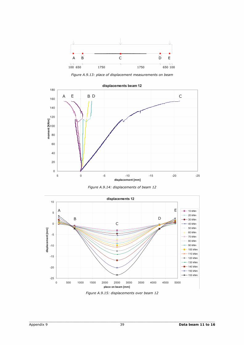
A B C D E
100 650 1750 1750 650 100
Figure A.9.13: place of displacement measurements on beam
displacements beam12
0
20
40
60
80
100
120
140
160
180
-25-20-15-10-505displacement [mm]
mom
ent[kNm]
CA B DE
Figure A.9.14: displacements of beam 12
displacements 12
-25
-20
-15
-10
-5
0
5
10
0 500 1000 1500 2000 2500 3000 3500 4000 4500 5000place on beam [mm]
displacement[mm]
10 kNm
20 kNm
30 kNm
40 kNm
50 kNm
60 kNm
70 kNm
80 kNm
90 kNm
100 kNm
110 kNm
120 kNm
130 kNm
140 kNm
150 kNm
155 kNm
A
BC
D
E
Figure A.9.15: displacements over beam 12
_________________________________________________________________________________________ Appendix 9 40 Data beam 11 to 16
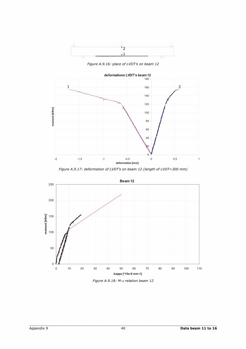
21
Figure A.9.16: place of LVDT’s on beam 12
deformations LVDT's beam12
0
20
40
60
80
100
120
140
160
180
-2 -1.5 -1 -0.5 0 0.5 1deformation [mm]
mom
ent[kNm]
1 2
Figure A.9.17: deformation of LVDT’s on beam 12 (length of LVDT=300 mm)
Beam12
0
50
100
150
200
250
0 10 20 30 40 50 60 70 80 90 100 110
kappa [*10e-6 mm-1]
moment[kNm]
Figure A.9.18: M-κ relation beam 12
_________________________________________________________________________________________ Appendix 9 41 Data beam 11 to 16
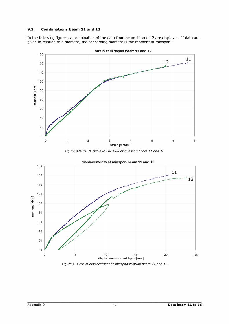
9.3 Combinations beam 11 and 12 In the following figures, a combination of the data from beam 11 and 12 are displayed. If data are given in relation to a moment, the concerning moment is the moment at midspan.
strain at midspan beam11 and 12
0
20
40
60
80
100
120
140
160
180
0 1 2 3 4 5 6 7strain [mm/m]
mom
ent[kNm]
1211
Figure A.9.19: M-strain in FRP EBR at midspan beam 11 and 12
displacements at midspan beam11 and 12
0
20
40
60
80
100
120
140
160
180
-25-20-15-10-50displacements at midspan [mm]
moment[kNm]
11
12
Figure A.9.20: M-displacement at midspan relation beam 11 and 12
_________________________________________________________________________________________ Appendix 9 42 Data beam 11 to 16
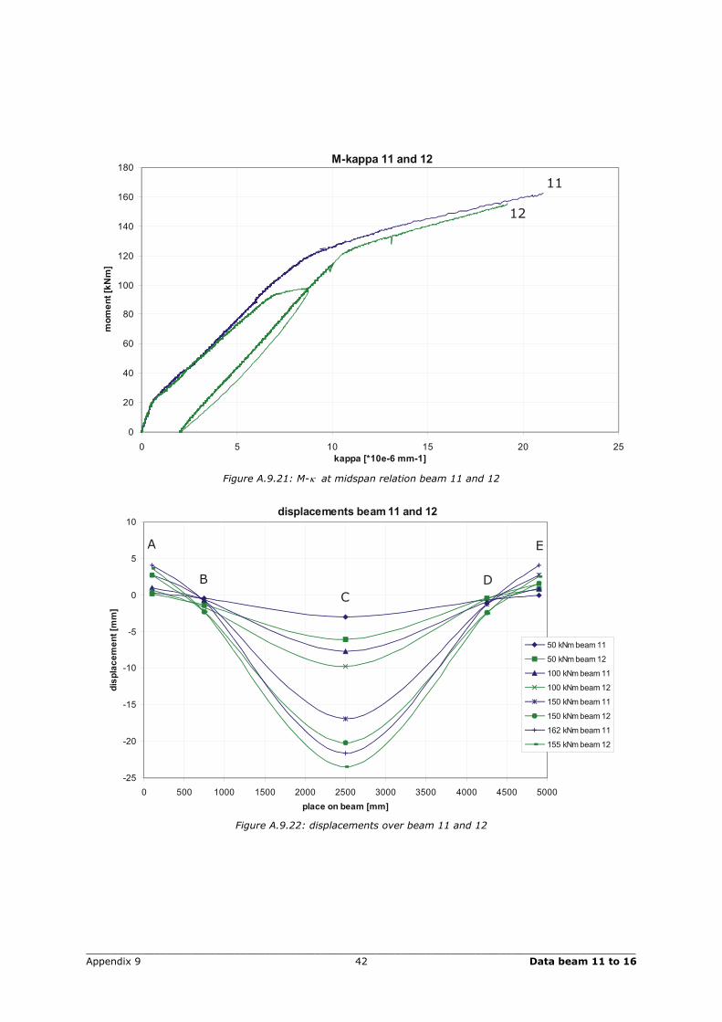
M-kappa 11 and 12
0
20
40
60
80
100
120
140
160
180
0 5 10 15 20 25kappa [*10e-6 mm-1]
moment[kNm]
11
12
Figure A.9.21: M-κ at midspan relation beam 11 and 12
displacements beam11 and 12
-25
-20
-15
-10
-5
0
5
10
0 500 1000 1500 2000 2500 3000 3500 4000 4500 5000place on beam [mm]
displacement[mm]
50 kNmbeam11
50 kNmbeam12
100 kNmbeam11
100 kNmbeam12
150 kNmbeam11
150 kNmbeam12
162 kNmbeam11
155 kNmbeam12
A
BC
D
E
Figure A.9.22: displacements over beam 11 and 12
_________________________________________________________________________________________ Appendix 9 43 Data beam 11 to 16
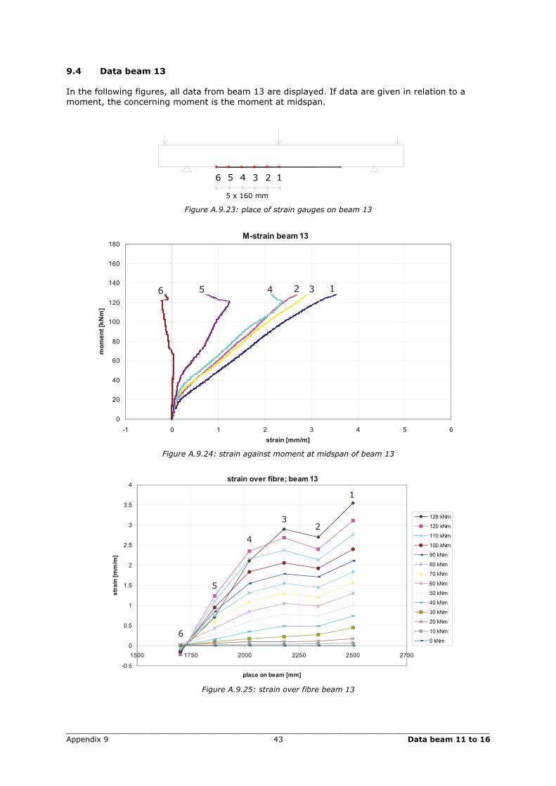
9.4 Data beam 13 In the following figures, all data from beam 13 are displayed. If data are given in relation to a moment, the concerning moment is the moment at midspan.
5 x 160 mm
123456
Figure A.9.23: place of strain gauges on beam 13
M-strain beam13
0
20
40
60
80
100
120
140
160
180
-1 0 1 2 3 4 5 6strain [mm/m]
mom
ent[kNm]
6 5 4 32 1
Figure A.9.24: strain against moment at midspan of beam 13
strain over fibre; beam13
-0.5
0
0.5
1
1.5
2
2.5
3
3.5
4
1500 1750 2000 2250 2500 2750
place on beam [mm]
strain[mm/m]
128 kNm
120 kNm
110 kNm
100 kNm
90 kNm
80 kNm
70 kNm
60 kNm
50 kNm
40 kNm
30 kNm
20 kNm
10 kNm
0 kNm6
5
4
32
1
Figure A.9.25: strain over fibre beam 13
_________________________________________________________________________________________ Appendix 9 44 Data beam 11 to 16
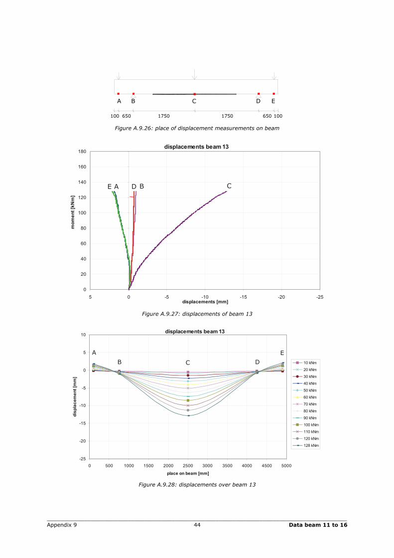
A B C D E
100 650 1750 1750 650 100
Figure A.9.26: place of displacement measurements on beam
displacements beam13
0
20
40
60
80
100
120
140
160
180
-25-20-15-10-505displacements [mm]
mom
ent[kNm]
E A D B C
Figure A.9.27: displacements of beam 13
displacements beam13
-25
-20
-15
-10
-5
0
5
10
0 500 1000 1500 2000 2500 3000 3500 4000 4500 5000
place on beam [mm]
displacement[mm]
10 kNm
20 kNm
30 kNm
40 kNm
50 kNm
60 kNm
70 kNm
80 kNm
90 kNm
100 kNm
110 kNm
120 kNm
128 kNm
A
B C D
E
Figure A.9.28: displacements over beam 13
_________________________________________________________________________________________ Appendix 9 45 Data beam 11 to 16
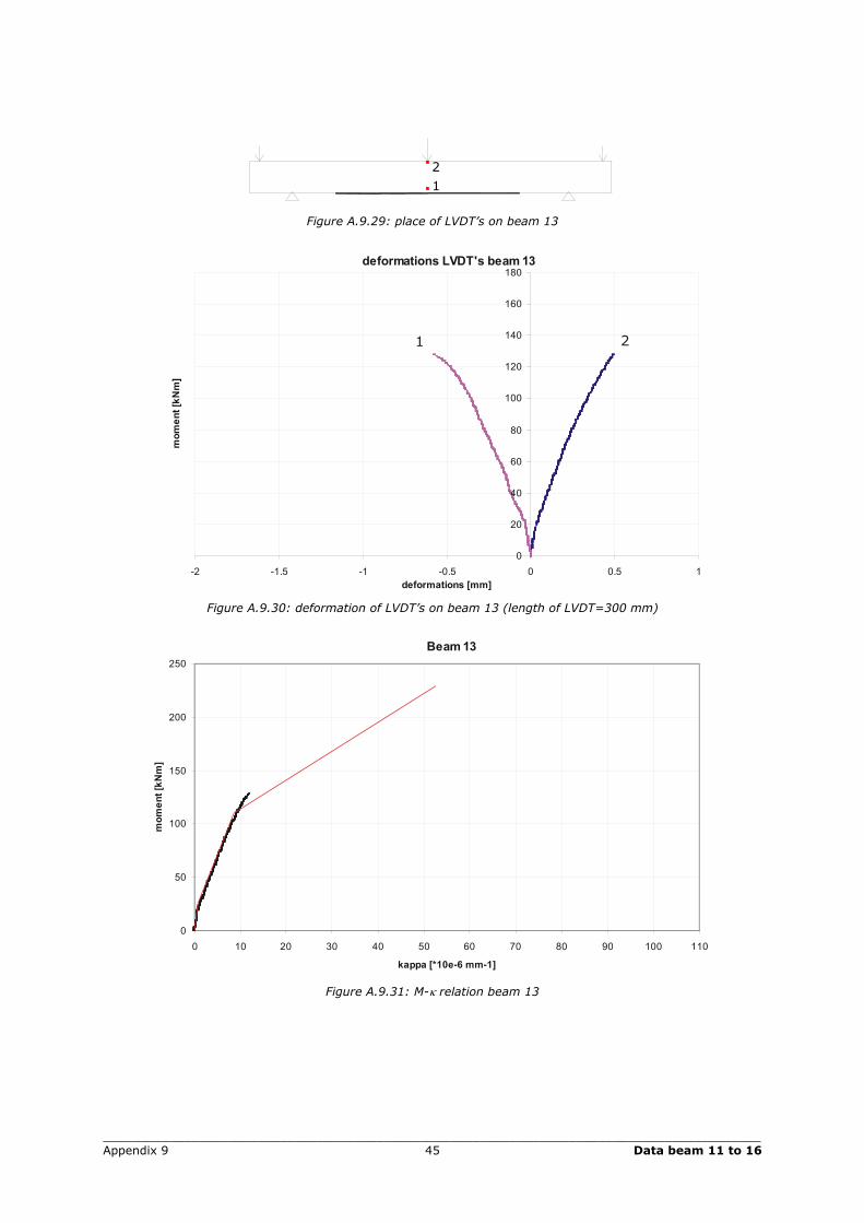
21
Figure A.9.29: place of LVDT’s on beam 13
deformations LVDT's beam13
0
20
40
60
80
100
120
140
160
180
-2 -1.5 -1 -0.5 0 0.5 1deformations [mm]
moment[kNm]
1 2
Figure A.9.30: deformation of LVDT’s on beam 13 (length of LVDT=300 mm)
Beam13
0
50
100
150
200
250
0 10 20 30 40 50 60 70 80 90 100 110
kappa [*10e-6 mm-1]
moment[kNm]
Figure A.9.31: M-κ relation beam 13
_________________________________________________________________________________________ Appendix 9 46 Data beam 11 to 16
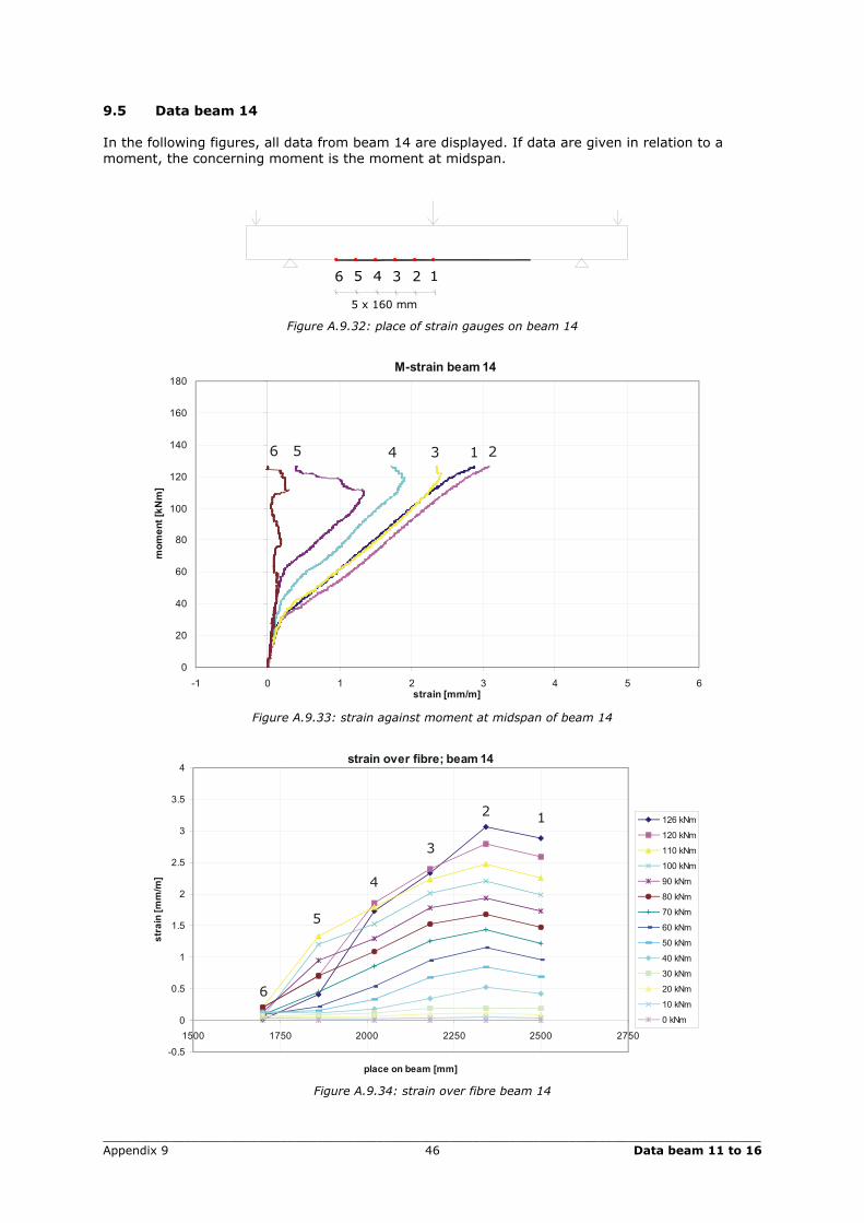
9.5 Data beam 14 In the following figures, all data from beam 14 are displayed. If data are given in relation to a moment, the concerning moment is the moment at midspan.
5 x 160 mm
123456
Figure A.9.32: place of strain gauges on beam 14
M-strain beam14
0
20
40
60
80
100
120
140
160
180
-1 0 1 2 3 4 5 6strain [mm/m]
moment[kNm]
6 5 4 3 21
Figure A.9.33: strain against moment at midspan of beam 14
strain over fibre; beam14
-0.5
0
0.5
1
1.5
2
2.5
3
3.5
4
1500 1750 2000 2250 2500 2750
place on beam [mm]
strain[mm/m]
126 kNm
120 kNm
110 kNm
100 kNm
90 kNm
80 kNm
70 kNm
60 kNm
50 kNm
40 kNm
30 kNm
20 kNm
10 kNm
0 kNm
12
3
4
5
6
Figure A.9.34: strain over fibre beam 14
_________________________________________________________________________________________ Appendix 9 47 Data beam 11 to 16
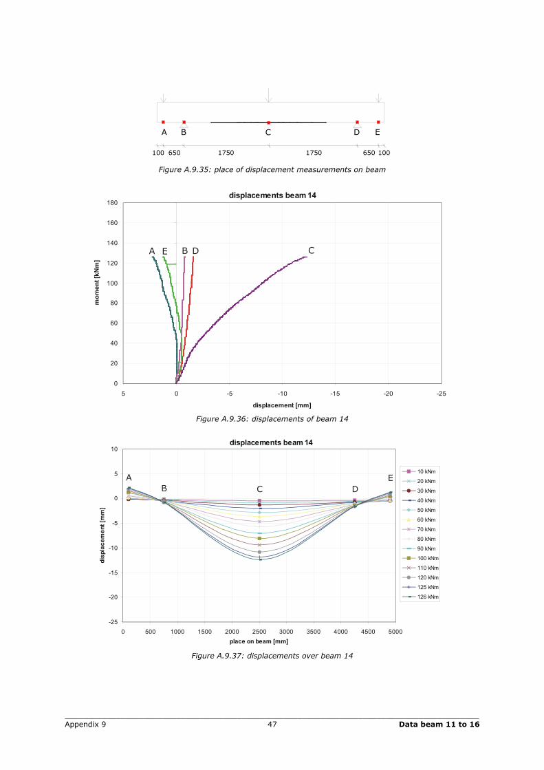
A B C D E
100 650 1750 1750 650 100
Figure A.9.35: place of displacement measurements on beam
displacements beam14
0
20
40
60
80
100
120
140
160
180
-25-20-15-10-505
displacement [mm]
moment[kNm]
EA DB C
Figure A.9.36: displacements of beam 14
displacements beam14
-25
-20
-15
-10
-5
0
5
10
0 500 1000 1500 2000 2500 3000 3500 4000 4500 5000place on beam [mm]
displacement[mm]
10 kNm
20 kNm
30 kNm
40 kNm
50 kNm
60 kNm
70 kNm
80 kNm
90 kNm
100 kNm
110 kNm
120 kNm
125 kNm
126 kNm
AB C D
E
Figure A.9.37: displacements over beam 14
_________________________________________________________________________________________ Appendix 9 48 Data beam 11 to 16
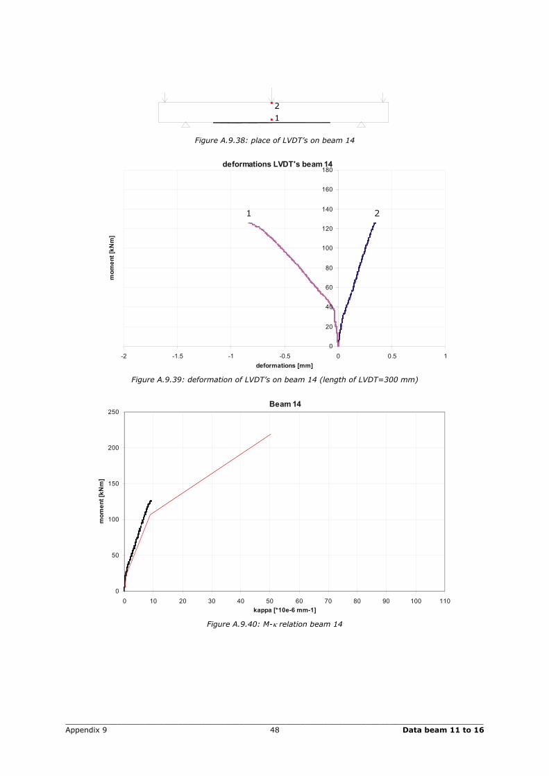
21
Figure A.9.38: place of LVDT’s on beam 14
deformations LVDT's beam14
0
20
40
60
80
100
120
140
160
180
-2 -1.5 -1 -0.5 0 0.5 1deformations [mm]
mom
ent[kNm]
1 2
Figure A.9.39: deformation of LVDT’s on beam 14 (length of LVDT=300 mm)
Beam14
0
50
100
150
200
250
0 10 20 30 40 50 60 70 80 90 100 110kappa [*10e-6 mm-1]
mom
ent[kNm]
Figure A.9.40: M-κ relation beam 14
_________________________________________________________________________________________ Appendix 9 49 Data beam 11 to 16
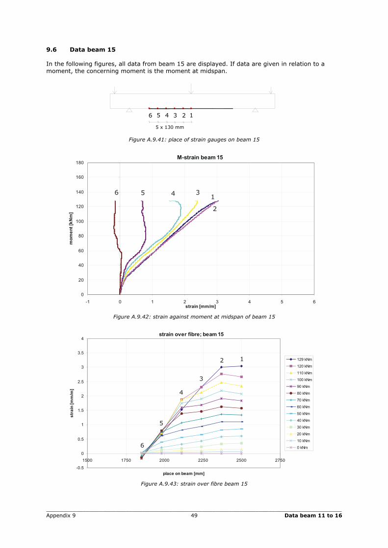
9.6 Data beam 15 In the following figures, all data from beam 15 are displayed. If data are given in relation to a moment, the concerning moment is the moment at midspan.
6 5 4 3 2 1
5 x 130 mm
Figure A.9.41: place of strain gauges on beam 15
M-strain beam15
0
20
40
60
80
100
120
140
160
180
-1 0 1 2 3 4 5 6strain [mm/m]
mom
ent[kNm] 2
13456
Figure A.9.42: strain against moment at midspan of beam 15
strain over fibre; beam15
-0.5
0
0.5
1
1.5
2
2.5
3
3.5
4
1500 1750 2000 2250 2500 2750
place on beam [mm]
strain[mm/m]
129 kNm
120 kNm
110 kNm
100 kNm
90 kNm
80 kNm
70 kNm
60 kNm
50 kNm
40 kNm
30 kNm
20 kNm
10 kNm
0 kNm
12
3
4
5
6
Figure A.9.43: strain over fibre beam 15
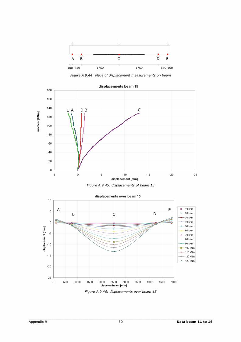
_________________________________________________________________________________________ Appendix 9 50 Data beam 11 to 16
A B C D E
100 650 1750 1750 650 100
Figure A.9.44: place of displacement measurements on beam
displacements beam15
0
20
40
60
80
100
120
140
160
180
-25-20-15-10-505displacement [mm]
moment[kNm] E A D B C
Figure A.9.45: displacements of beam 15
displacements over beam15
-25
-20
-15
-10
-5
0
5
10
0 500 1000 1500 2000 2500 3000 3500 4000 4500 5000place on beam [mm]
displacement[mm]
10 kNm
20 kNm
30 kNm
40 kNm
50 kNm
60 kNm
70 kNm
80 kNm
90 kNm
100 kNm
110 kNm
120 kNm
129 kNm
AB C D
E
Figure A.9.46: displacements over beam 15
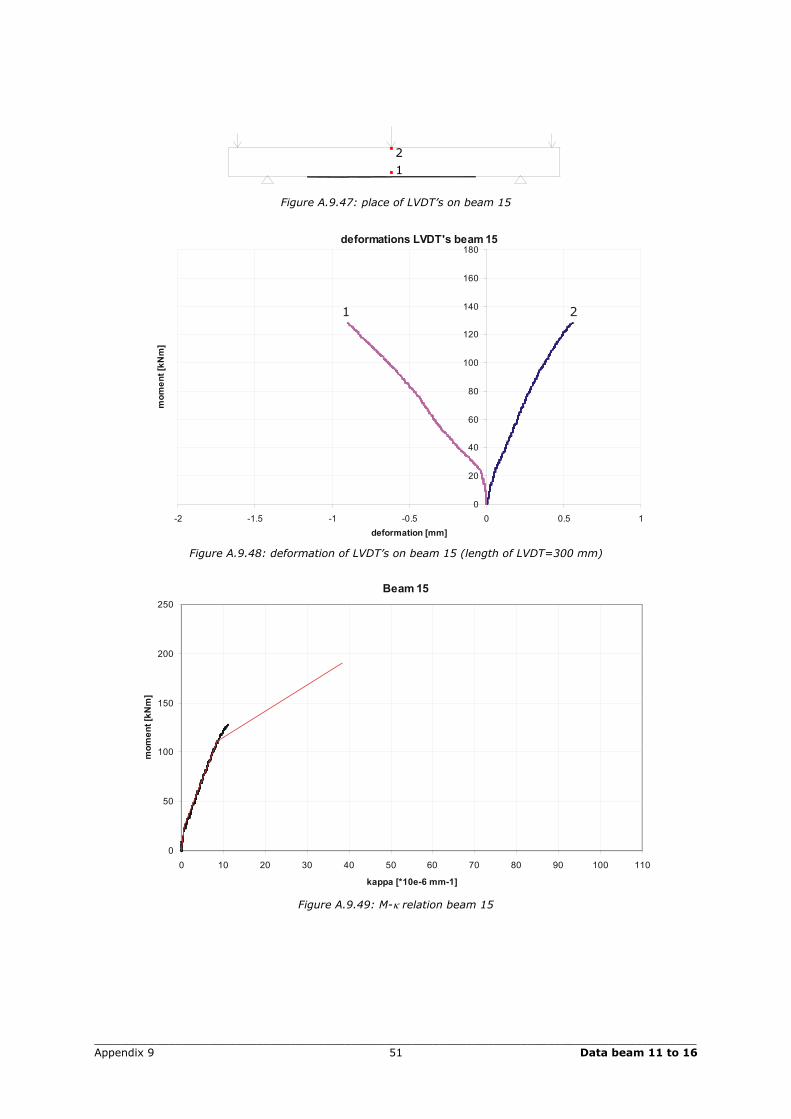
_________________________________________________________________________________________ Appendix 9 51 Data beam 11 to 16
21
Figure A.9.47: place of LVDT’s on beam 15
deformations LVDT's beam15
0
20
40
60
80
100
120
140
160
180
-2 -1.5 -1 -0.5 0 0.5 1deformation [mm]
mom
ent[kNm]
1 2
Figure A.9.48: deformation of LVDT’s on beam 15 (length of LVDT=300 mm)
Beam15
0
50
100
150
200
250
0 10 20 30 40 50 60 70 80 90 100 110
kappa [*10e-6 mm-1]
moment[kNm]
Figure A.9.49: M-κ relation beam 15
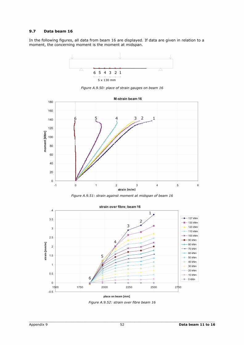
_________________________________________________________________________________________ Appendix 9 52 Data beam 11 to 16
9.7 Data beam 16 In the following figures, all data from beam 16 are displayed. If data are given in relation to a moment, the concerning moment is the moment at midspan.
6 5 4 3 2 1
5 x 130 mm
Figure A.9.50: place of strain gauges on beam 16
M-strain beam16
0
20
40
60
80
100
120
140
160
180
-1 0 1 2 3 4 5 6strain [m/m]
mom
ent[kNm]
6 5 4 3 2 1
Figure A.9.51: strain against moment at midspan of beam 16
strain over fibre; beam16
-0.5
0
0.5
1
1.5
2
2.5
3
3.5
4
1500 1750 2000 2250 2500 2750
place on beam [mm]
strain[mm/m]
137 kNm
130 kNm
120 kNm
110 kNm
100 kNm
90 kNm
80 kNm
70 kNm
60 kNm
50 kNm
40 kNm
30 kNm
20 kNm
10 kNm
0 kNm
1
23
4
5
6
Figure A.9.52: strain over fibre beam 16
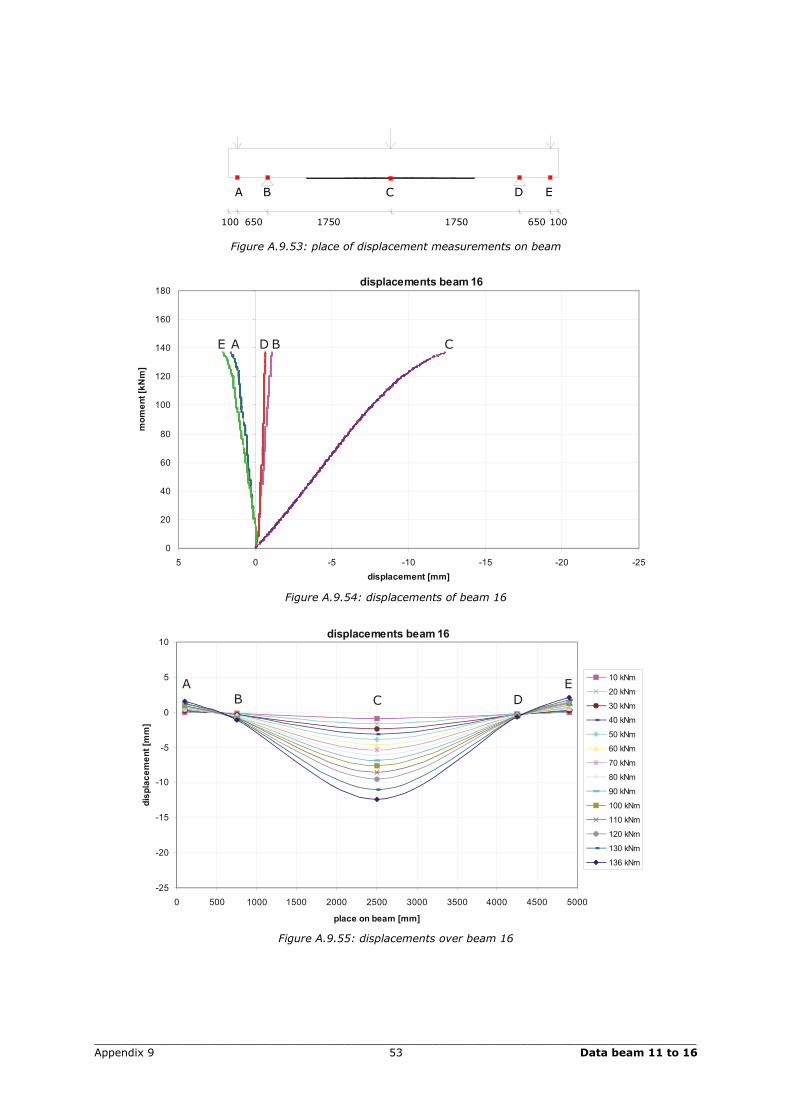
_________________________________________________________________________________________ Appendix 9 53 Data beam 11 to 16
A B C D E
100 650 1750 1750 650 100
Figure A.9.53: place of displacement measurements on beam
displacements beam16
0
20
40
60
80
100
120
140
160
180
-25-20-15-10-505displacement [mm]
mom
ent[kNm]
E A D B C
Figure A.9.54: displacements of beam 16
displacements beam16
-25
-20
-15
-10
-5
0
5
10
0 500 1000 1500 2000 2500 3000 3500 4000 4500 5000
place on beam [mm]
displacement[mm]
10 kNm
20 kNm
30 kNm
40 kNm
50 kNm
60 kNm
70 kNm
80 kNm
90 kNm
100 kNm
110 kNm
120 kNm
130 kNm
136 kNm
AB C D
E
Figure A.9.55: displacements over beam 16
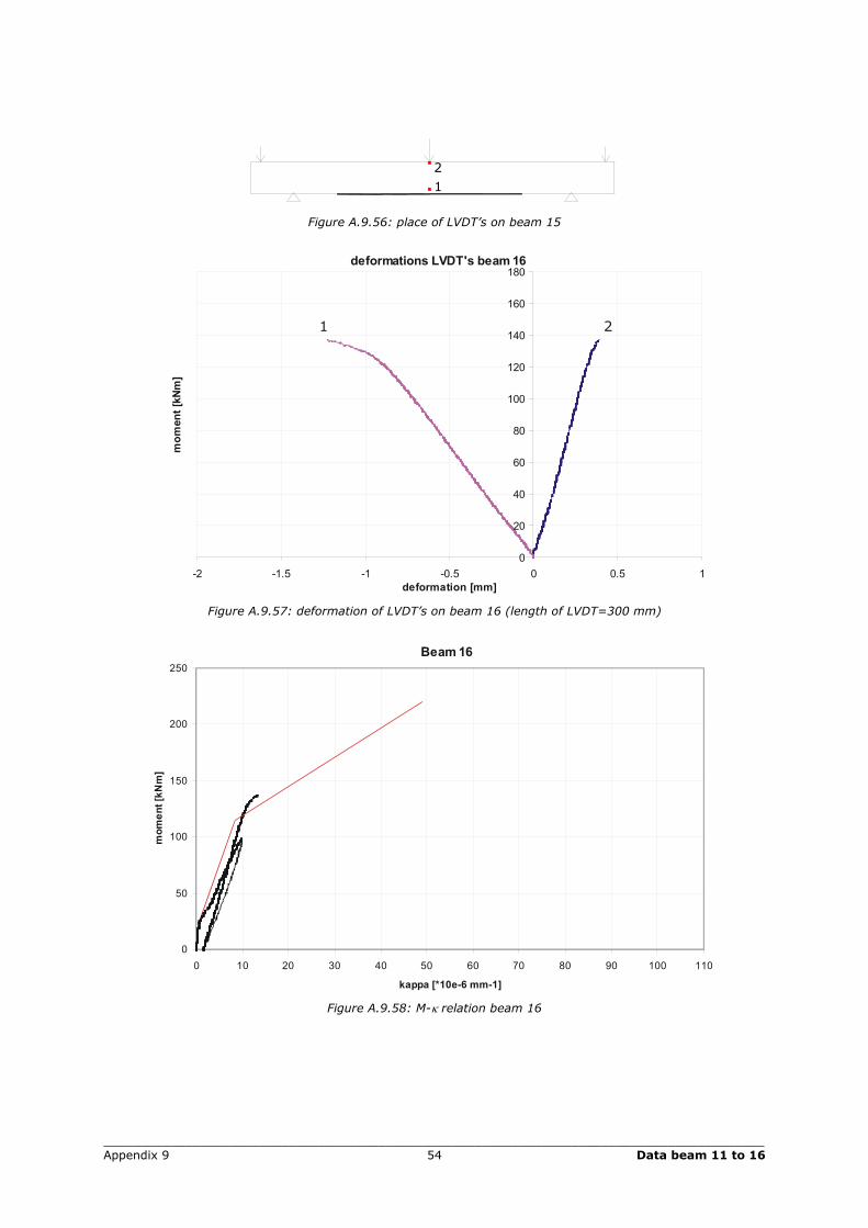
_________________________________________________________________________________________ Appendix 9 54 Data beam 11 to 16
21
Figure A.9.56: place of LVDT’s on beam 15
deformations LVDT's beam16
0
20
40
60
80
100
120
140
160
180
-2 -1.5 -1 -0.5 0 0.5 1deformation [mm]
mom
ent[kNm]
1 2
Figure A.9.57: deformation of LVDT’s on beam 16 (length of LVDT=300 mm)
Beam16
0
50
100
150
200
250
0 10 20 30 40 50 60 70 80 90 100 110
kappa [*10e-6 mm-1]
moment[kNm]
Figure A.9.58: M-κ relation beam 16
_________________________________________________________________________________________ Appendix 9 55 Data beam 11 to 16
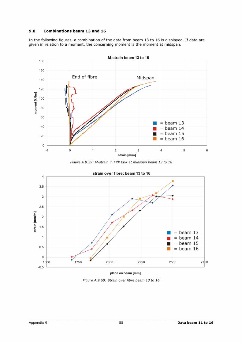
9.8 Combinations beam 13 and 16 In the following figures, a combination of the data from beam 13 to 16 is displayed. If data are given in relation to a moment, the concerning moment is the moment at midspan.
M-strain beam13 to 16
0
20
40
60
80
100
120
140
160
180
-1 0 1 2 3 4 5 6strain [m/m]
mom
ent[kNm]
End of fibre Midspan
= beam 13= beam 14= beam 15= beam 16
Figure A.9.59: M-strain in FRP EBR at midspan beam 13 to 16
strain over fibre; beam13 to 16
-0.5
0
0.5
1
1.5
2
2.5
3
3.5
4
1500 1750 2000 2250 2500 2750
place on beam [mm]
strain[mm/m]
= beam 13= beam 14= beam 15= beam 16
Figure A.9.60: Strain over fibre beam 13 to 16
_________________________________________________________________________________________ Appendix 9 56 Data beam 11 to 16
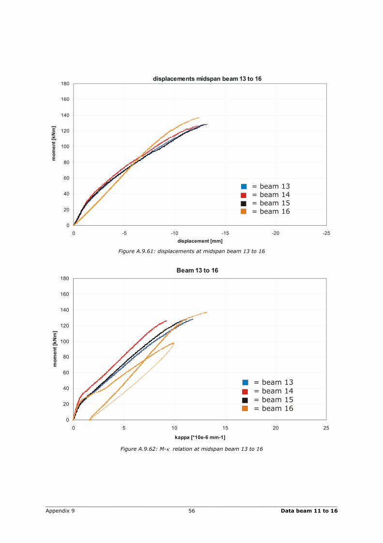
displacements midspan beam13 to 16
0
20
40
60
80
100
120
140
160
180
-25-20-15-10-50displacement [mm]
moment[kNm]
= beam 13= beam 14= beam 15= beam 16
Figure A.9.61: displacements at midspan beam 13 to 16
Beam13 to 16
0
20
40
60
80
100
120
140
160
180
0 5 10 15 20 25
kappa [*10e-6 mm-1]
moment[kNm]
= beam 13= beam 14= beam 15= beam 16
Figure A.9.62: M-κ relation at midspan beam 13 to 16
_________________________________________________________________________________________ Appendix 10 57 ESPI measurement beam 14
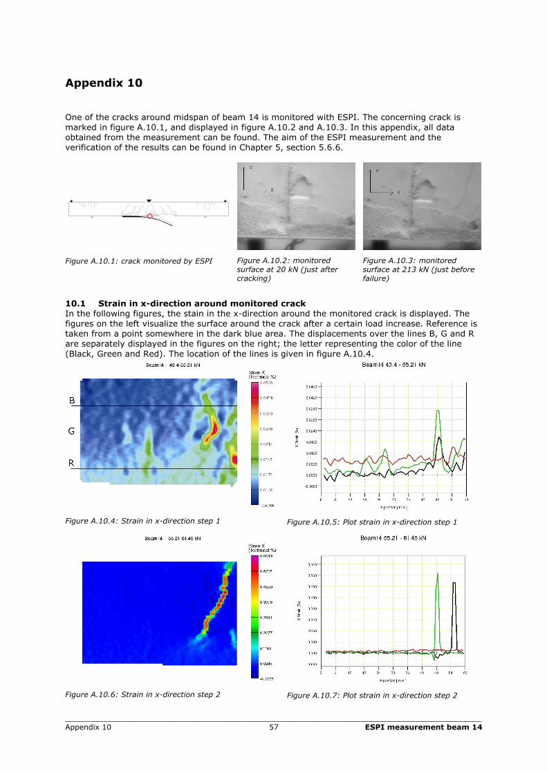
Appendix 10 One of the cracks around midspan of beam 14 is monitored with ESPI. The concerning crack is marked in figure A.10.1, and displayed in figure A.10.2 and A.10.3. In this appendix, all data obtained from the measurement can be found. The aim of the ESPI measurement and the verification of the results can be found in Chapter 5, section 5.6.6.
Figure A.10.1: crack monitored by ESPI
Figure A.10.2: monitored surface at 20 kN (just after cracking)
Figure A.10.3: monitored surface at 213 kN (just before failure)
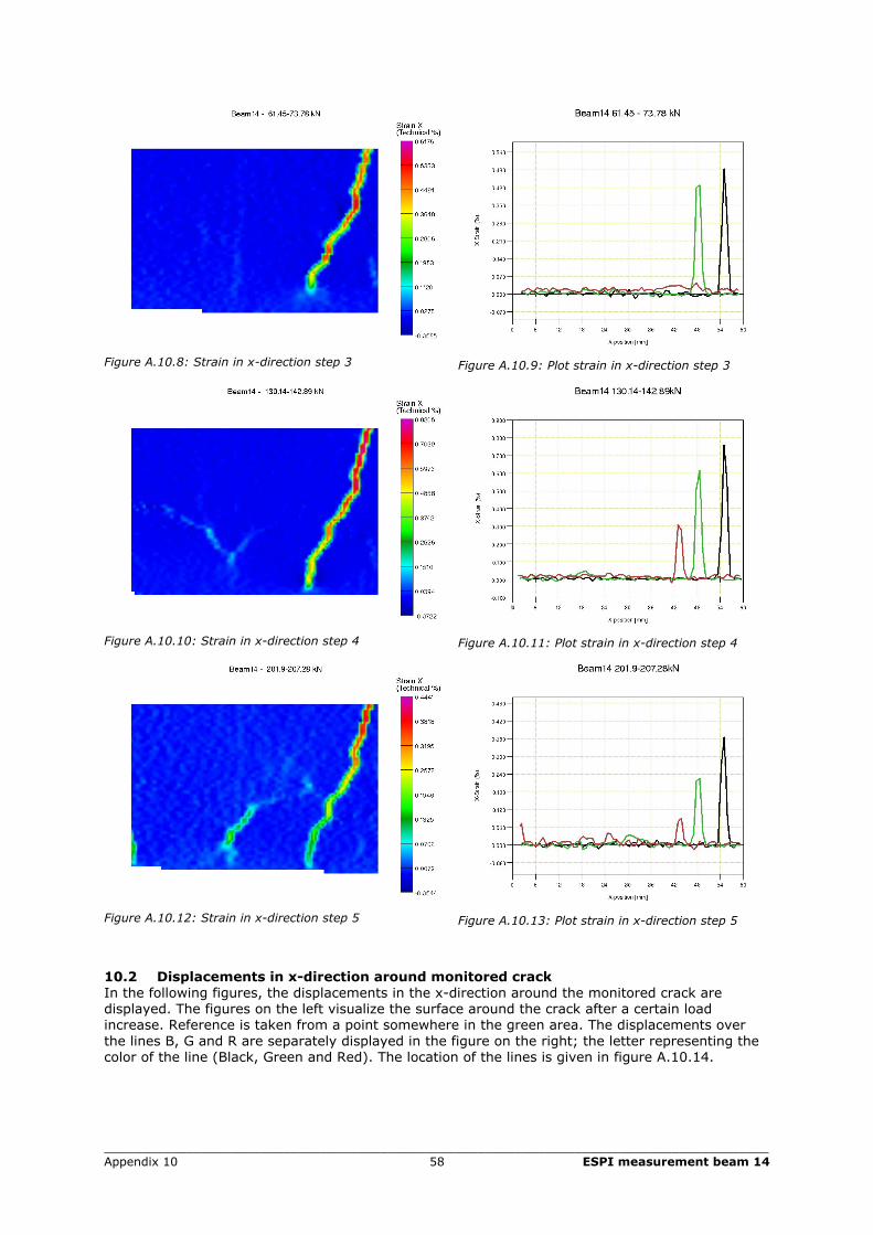
10.1 Strain in x-direction around monitored crack In the following figures, the stain in the x-direction around the monitored crack is displayed. The figures on the left visualize the surface around the crack after a certain load increase. Reference is taken from a point somewhere in the dark blue area. The displacements over the lines B, G and R are separately displayed in the figures on the right; the letter representing the color of the line (Black, Green and Red). The location of the lines is given in figure A.10.4.
Figure A.10.4: Strain in x-direction step 1
Figure A.10.5: Plot strain in x-direction step 1
Figure A.10.6: Strain in x-direction step 2
Figure A.10.7: Plot strain in x-direction step 2
_________________________________________________________________________________________ Appendix 10 58 ESPI measurement beam 14
Figure A.10.8: Strain in x-direction step 3
Figure A.10.9: Plot strain in x-direction step 3
Figure A.10.10: Strain in x-direction step 4
Figure A.10.11: Plot strain in x-direction step 4
Figure A.10.12: Strain in x-direction step 5
Figure A.10.13: Plot strain in x-direction step 5
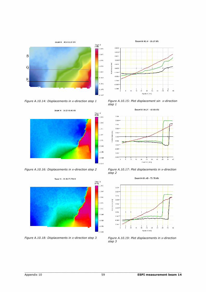
10.2 Displacements in x-direction around monitored crack In the following figures, the displacements in the x-direction around the monitored crack are displayed. The figures on the left visualize the surface around the crack after a certain load increase. Reference is taken from a point somewhere in the green area. The displacements over the lines B, G and R are separately displayed in the figure on the right; the letter representing the color of the line (Black, Green and Red). The location of the lines is given in figure A.10.14.
_________________________________________________________________________________________ Appendix 10 59 ESPI measurement beam 14
Figure A.10.14: Displacements in x-direction step 1
Figure A.10.15: Plot displacement sin x-direction step 1
Figure A.10.16: Displacements in x-direction step 2
Figure A.10.17: Plot displacements in x-direction step 2
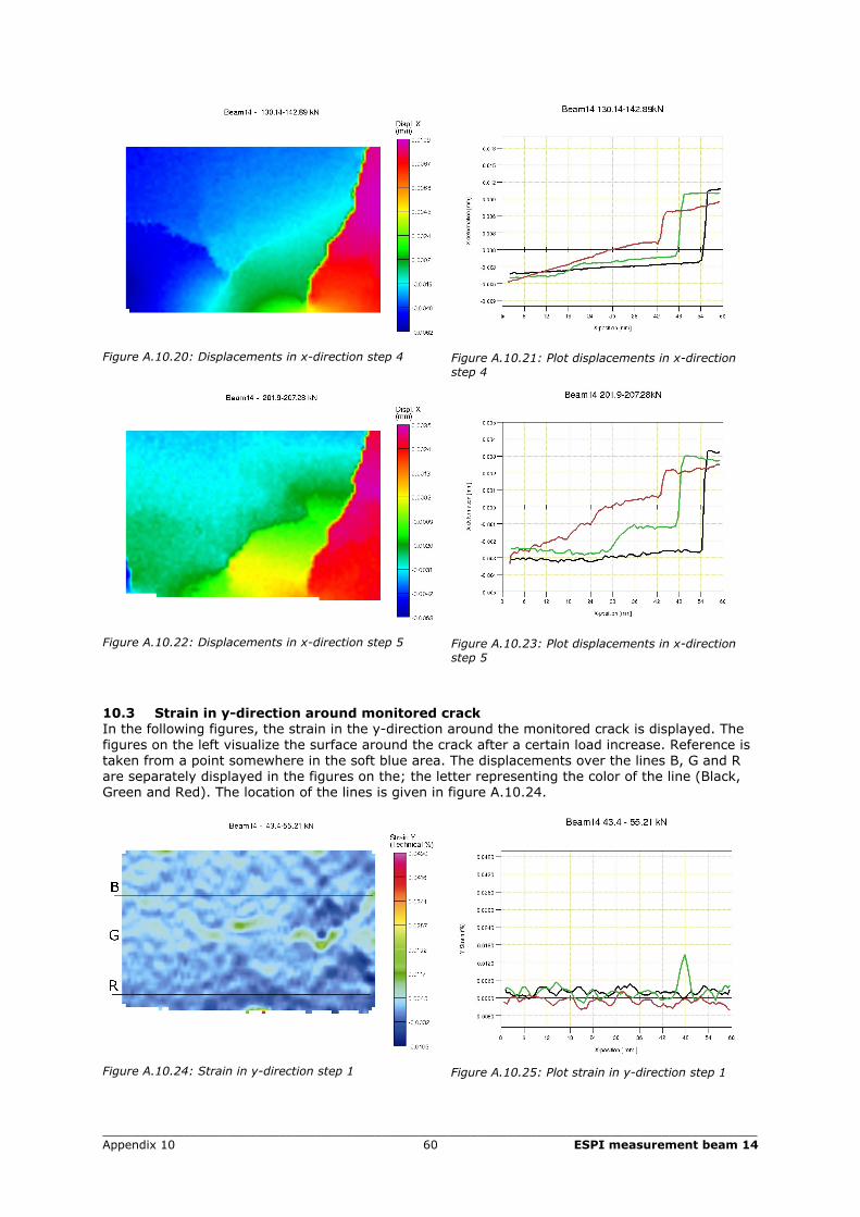
Figure A.10.18: Displacements in x-direction step 3
Figure A.10.19: Plot displacements in x-direction step 3
_________________________________________________________________________________________ Appendix 10 60 ESPI measurement beam 14
Figure A.10.20: Displacements in x-direction step 4
Figure A.10.21: Plot displacements in x-direction step 4
Figure A.10.22: Displacements in x-direction step 5
Figure A.10.23: Plot displacements in x-direction step 5
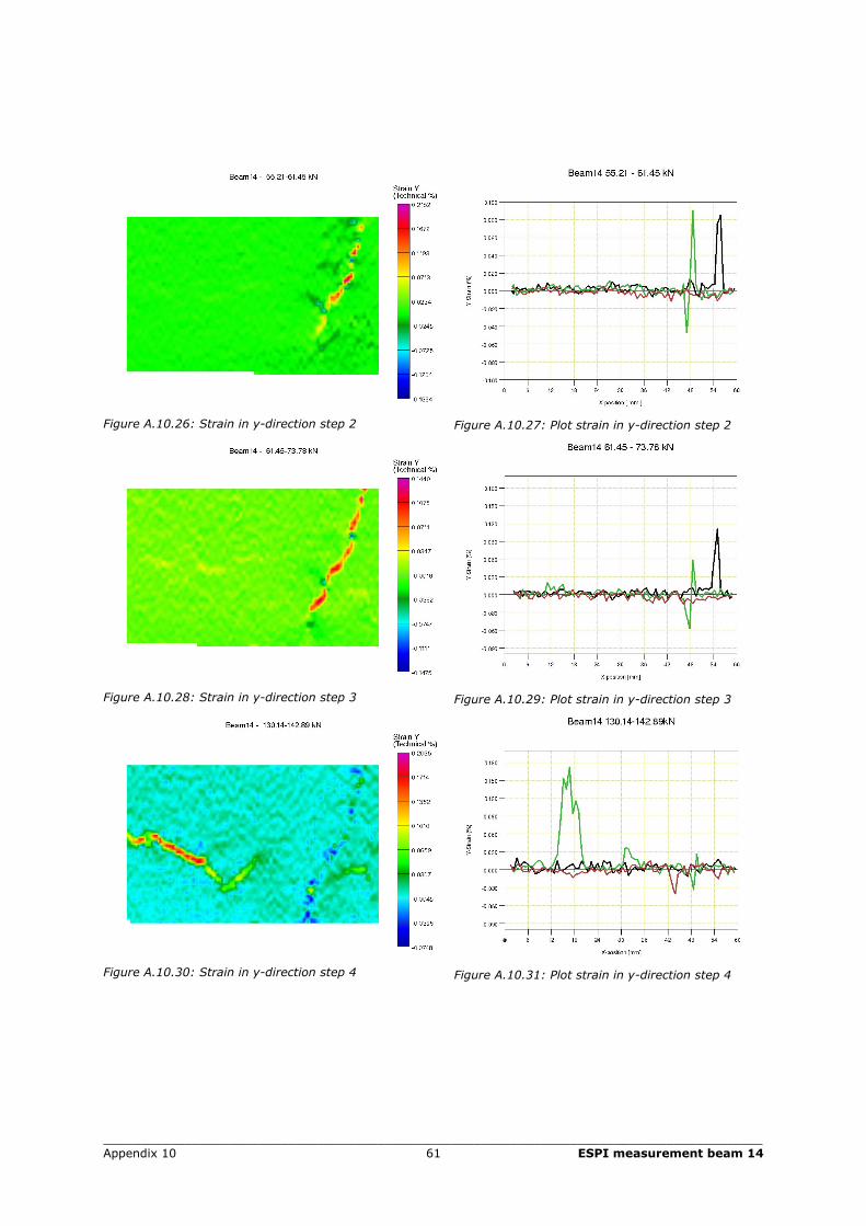
10.3 Strain in y-direction around monitored crack In the following figures, the strain in the y-direction around the monitored crack is displayed. The figures on the left visualize the surface around the crack after a certain load increase. Reference is taken from a point somewhere in the soft blue area. The displacements over the lines B, G and R are separately displayed in the figures on the; the letter representing the color of the line (Black, Green and Red). The location of the lines is given in figure A.10.24.
Figure A.10.24: Strain in y-direction step 1
Figure A.10.25: Plot strain in y-direction step 1
_________________________________________________________________________________________ Appendix 10 61 ESPI measurement beam 14
Figure A.10.26: Strain in y-direction step 2
Figure A.10.27: Plot strain in y-direction step 2
Figure A.10.28: Strain in y-direction step 3
Figure A.10.29: Plot strain in y-direction step 3
Figure A.10.30: Strain in y-direction step 4
Figure A.10.31: Plot strain in y-direction step 4
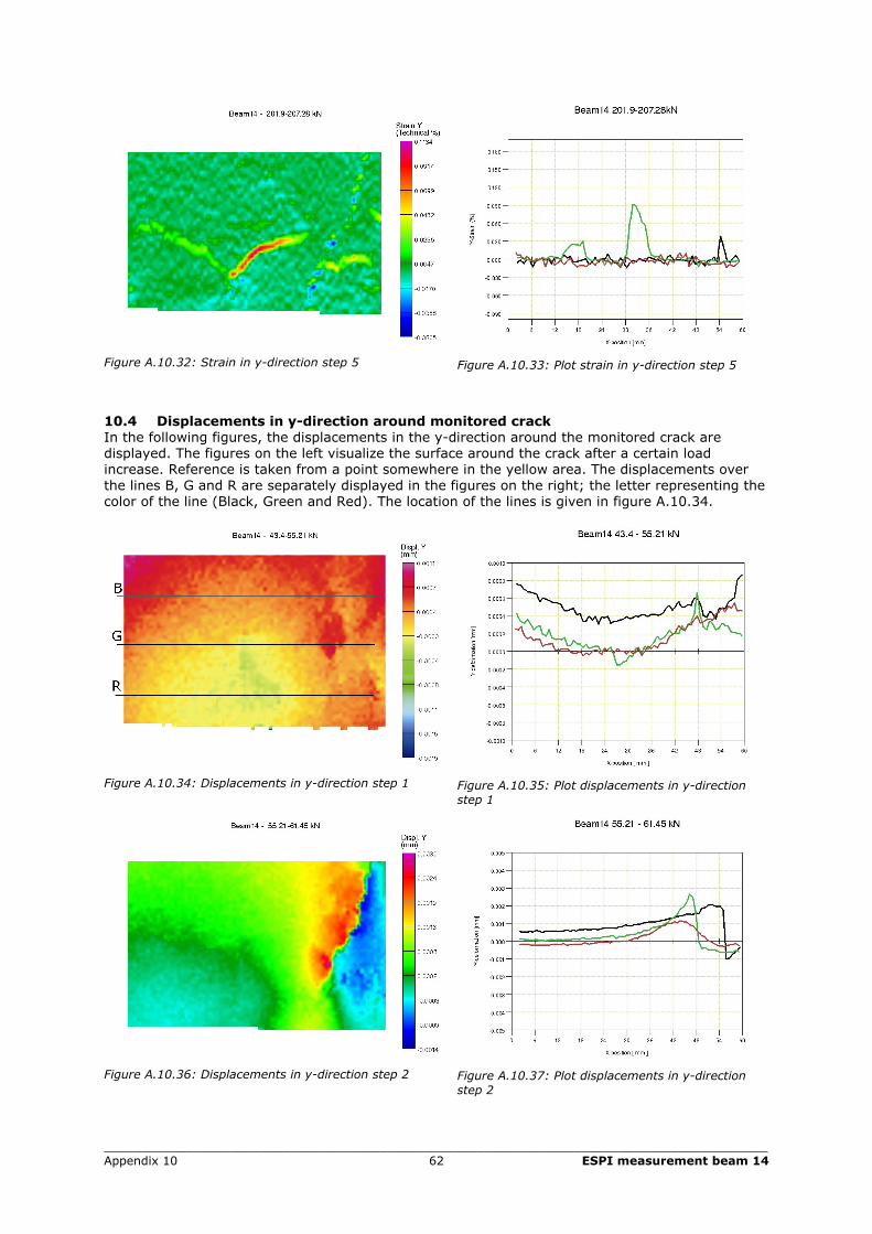
_________________________________________________________________________________________ Appendix 10 62 ESPI measurement beam 14
Figure A.10.32: Strain in y-direction step 5
Figure A.10.33: Plot strain in y-direction step 5
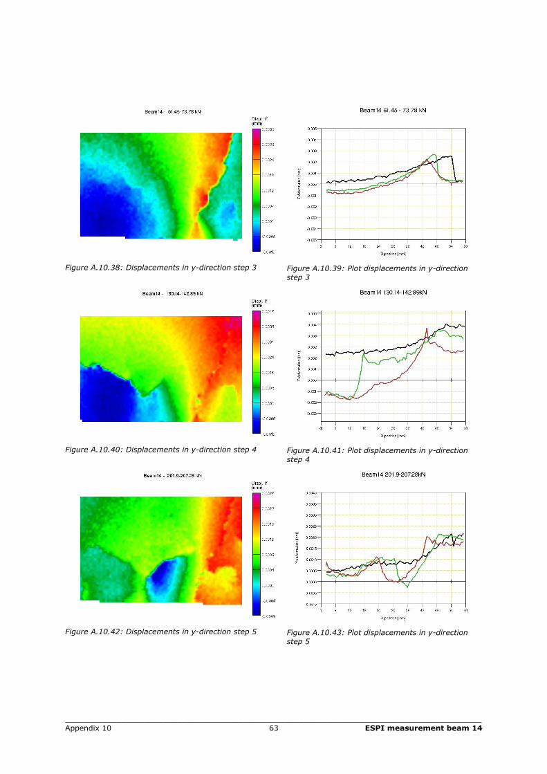
10.4 Displacements in y-direction around monitored crack In the following figures, the displacements in the y-direction around the monitored crack are displayed. The figures on the left visualize the surface around the crack after a certain load increase. Reference is taken from a point somewhere in the yellow area. The displacements over the lines B, G and R are separately displayed in the figures on the right; the letter representing the color of the line (Black, Green and Red). The location of the lines is given in figure A.10.34.
Figure A.10.34: Displacements in y-direction step 1
Figure A.10.35: Plot displacements in y-direction step 1
Figure A.10.36: Displacements in y-direction step 2
Figure A.10.37: Plot displacements in y-direction step 2
_________________________________________________________________________________________ Appendix 10 63 ESPI measurement beam 14
Figure A.10.38: Displacements in y-direction step 3
Figure A.10.39: Plot displacements in y-direction step 3
Figure A.10.40: Displacements in y-direction step 4
Figure A.10.41: Plot displacements in y-direction step 4
Figure A.10.42: Displacements in y-direction step 5
Figure A.10.43: Plot displacements in y-direction step 5


![[13]Influence of the dispersion map on limitations due to cross-phase modulation in wdm multispan transmission systems](https://img.pdfslide.net/doc/110x75/577cd9b91a28ab9e78a4060e/13influence-of-the-dispersion-map-on-limitations-due-to-cross-phase-modulation.jpg)