EISCAT 3D: A Next-Generation European Radar … Radio Science Bulletin No 332 (March 2010) 75 EISCAT_3D: A Next-Generation European Radar System for Upper-Atmosphere and Geospace Research

The Radio Science Bulletin No 332 (March 2010) 75

EISCAT_3D: A Next-Generation European Radar System

for Upper-Atmosphere and Geospace Research

U.G. Wannberget al.

Abstract

The EISCAT Scientifi c Association, together with a number of collaborating institutions, has recently completed a feasibility and design study for an enhanced performance research radar facility to replace the existing EISCAT UHF and VHF systems. This study was supported by EU Sixth-Framework funding. The new radar retains the powerful multi-static geometry of the EISCAT UHF, but will employ phased arrays, direct-sampling receivers, and digital beamforming and beam steering. Design goals include, inter alia, a tenfold improvement in temporal and spatial resolution, an extension of the instantaneous measurement of full-vector ionospheric drift velocities from a single point to the entire altitude range of the radar, and an imaging capability to resolve small-scale structures. Prototype receivers and beamformers are currently being tested on a 48-element, 224 MHz array (the “Demonstrator”) erected at the Kiruna EISCAT site, using the EISCAT VHF transmitter as an illuminator.

1. Introduction

The radar systems of the European Incoherent Scatter Association (EISCAT) have provided the scientifi c

community with outstanding high-latitude data for more than 25 years. Observations made during this time have contributed to the opening of several new fi elds of research, e.g., the study of transient coherent echoes from the ionosphere, polar mesospheric summer echoes (PMSE), extremely narrow natural layers of ionization in the E region, and observations of micro-meteors interacting with the atmosphere. Many of these phenomena are spatially compact and of very short duration (tens of milliseconds or less), while others tend to occur under conditions of low electron density and/or very high electron-to-ion temperature ratio. Radar returns from these processes also frequently show a signifi cant degree of coherence.

The present EISCAT UHF and VHF systems, having been designed for incoherent-scatter conditions, are not really optimized for addressing these scientifi c challenges. In addition, the frequency band currently used by the multi-static UHF radar will soon be claimed by the UMTS900 third-generation mobile phone service in all the three EISCAT host countries, forcing the gradual closing down of the UHF system over a three-year period. There is thus a strong case for a new research radar system in the auroral zone.

In 2005, the EISCAT Association, Luleå University of Technology, Tromsø University, and the Rutherford

Correspondence should be directed to U. G. Wannberg via e-mail: [email protected]. U. G. Wannberg, L. Eliasson, J. Johansson, and I. Wolf are with the Swedish Institute of Space Physics, Box 812, SE-981 28 Kiruna, Sweden. H. Andersson, P. Bergqvist, I. Häggström, T. Iinatti, T. Laakso, R. Larsen, J. Markkanen, I. Marttala, M. Postila, E. Turunen, A. van Eyken, L.-G. Vanhainen, and A. Westman are with the EISCAT Scientifi c Association, Box 812, SE-981 28 Kiruna, Sweden. R. Behlke, V. Belyey, T. Grydeland, B. Gustavsson, and C. La Hoz are with the Auroral Observatory, University of Tromsø, N-9037, Tromsø, Norway. J. Borg, J. Delsing, J. Johansson, M. Larsmark, T. Lindgren, and M. Lundberg are with EISLAB, Luleå University of Technology, SE-971 87, Luleå, Sweden. I. Finch, R. A. Harrison, and D. McKay are with the Space Science and Technology Department, Rutherford Appleton

Laboratory, Chilton, Oxfordshire OX11 0QX, UK. W. Puccio is with the Swedish Institute of Space Physics, Box 537, SE-751 21 Uppsala, Sweden. T. Renkwitz is with the Institut für Atmosphärenphysik, D-18225, Kuhlungsborn, Germany. T. Grydeland is now at Discover Petroleum, Roald Amundsens Plass 1B, 9008 Tromsø, Norway. B. Gustavsson is now at the Department of Communication Systems, University of Lancaster, Lancaster LA1 4YR, UK. M. Postila is now at Sodankylä Geophysical Observatory, Tähteläntie 62, FIN-99600 Sodankylä, Finland. A. van Eyken is now at SRI International, 333 Ravenswood Avenue, Menlo Park, CA 94025, USA. This is one of the invited Reviews of Radio Science from Commission G

76 The Radio Science Bulletin No 332 (March 2010)

Appleton Laboratory (joined in 2008 by the Swedish Institute of Space Physics) therefore embarked on a four-year design and feasibility study for a new research radar facility with greatly enhanced performance. This was supported by European Union funding under the Sixth Framework Initiative. This facility would be capable of providing high-quality ionospheric and atmospheric parameters on an essentially continuous basis, as well as near-instantaneous response capabilities for users needing data to study unusual and unpredicted disturbances and phenomena in the high-latitude ionosphere and atmosphere. The study period ended on April 30, 2009. The present paper is a condensed summary of the results and recommendations from the study. A comprehensive report [1] was submitted to the EU FP6 Project Offi ce on June 14, 2009.

2. EISCAT_3D Performance Targets

Design targets for the new EISCAT_3D system [1] include:• A tenfold improvement in temporal and spatial resolution

relative to the current EISCAT systems. It will be possible to measure electron densities to better than 10% accuracy over the 100 to 300 km range in one second or less, even at 100 m altitude resolution.

• An extension of the instantaneous measurement of full-vector ionospheric drift velocities from a single point to the entire altitude range of the radar. It is planned to have at least fi ve beamformers running concurrently at the receive-only sites.

• Beam-pointing resolution of better than 0.625° in two orthogonal planes, with 10% (0.06°) pointing accuracy.

• Built-in imaging capabilities, offering a horizontal resolution of better than 20 m at 100 km altitude.

The transmitter system will be designed to provide better than 100 m line-of-sight resolution along the transmitted beam. The antenna arrays at the receiving sites will be designed to provide better than 150 m horizontal 3dB resolution at 100 km altitude everywhere in the multi-static fi eld of view.

3. System Confi guration

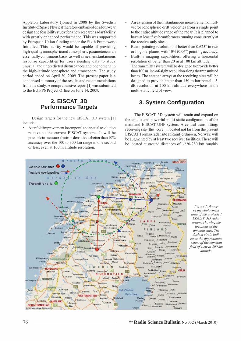
The EISCAT_3D system will retain and expand on the unique and powerful multi-static confi guration of the mainland EISCAT UHF system. A central transmitting/receiving site (the “core”), located not far from the present EISCAT Tromsø radar site at Ramfjordmoen, Norway, will be augmented by at least two receiver facilities. These will be located at ground distances of ~220-280 km roughly

Figure 1. A map of the deployment

area of the projected EISCAT_3D radar system, showing the

locations of the antenna sites. The dashed circle indi-

cates the approximate extent of the common fi eld of view at 300 km

altitude.


south and east of the core site, respectively (see Figure 1). Each receiving site will be equipped with a phased-array antenna and its associated receivers. These will be followed by a beamformer system capable of generating several simultaneous, independently steerable receiving beams that can intersect the beam from the central core at arbitrary altitudes between 200 and 800 km. Two additional receiving facilities, located at ground distances of ~90-120 km from the core on the same north-south and east-west baselines, will deliver three-dimensional data from the 70-250 km altitude range. This will thus provide truly simultaneous three-dimensional measurements over the entire vertical extent of the ionosphere for the fi rst time in the history of incoherent-scatter diagnostics. In addition, the transmitting/receiving site will also provide monostatic coverage into the ionospheric topside to beyond 2000 km altitude, where three-dimensional coverage is not required.

For optimum performance in low-electron-density

conditions, i.e., primarily at mesospheric and ionosphere topside altitudes, the EISCAT_3D system will use an operating frequency in the high VHF range. However, obtaining a coordinated allocation for a scientifi c radar system in this part of the spectrum has turned out to be a very nontrivial problem. In the ITU Radio Regulations, the entire 174-230 MHz frequency range is allocated to the Broadcasting Service on a primary basis and to various communication services on a secondary basis. The 230-240 MHz range is allocated to the fi xed and mobile services on a primary basis. In Europe, a slightly different scheme (the so-called Wiesbaden Agreement, WI95), based on proposals from CEPT and its subsidiary, the European Telecommunications Standards Institute (ETSI), has been adopted. Under WI95, the entire 174-240 MHz range is allocated to broadcasting. Frequencies above 235 MHz are shared with the military.

Following the transition from analog to digital terrestrial TV broadcasting in Europe, the 174-240 MHz range is now gradually being taken into use for digital audio broadcasting (T-DAB). The WI95 plan allocates one or more

frequency blocks for T-DAB to each European country. However, the actual implementation of the spectrum at the national level is delegated to the respective frequency administrations. This is fortunate, as the administrations are in fact free to also allocate spectrum to services other than those having a recognized status in a specifi c band, as long as this causes no interference to the primary service(s). In early 2008, the EISCAT_3D design study team therefore approached all three Nordic frequency administrations with a request to have 10 MHz of contiguous, coordinated bandwidth in the 225-240 MHz range allocated to the project. The Norwegian administration eventually responded by offering to allocate T-DAB blocks 13A-13D (229.928-236.632 MHz) for active use by the future EISCAT_3D core site on a noninterference basis, these blocks being unallocated in northern Norway. This offer was gratefully accepted by the EISCAT Scientifi c Association on December 17, 2008.

The spectrum slot proposed by the Norwegian

administration also turned out to be essentially unallocated in northern Sweden and northern Finland. Negotiations are currently in progress with the respective administrations, with the aim to obtain Nordic-wide protection of at least 230.0-236.5 MHz for reception.

The fully populated core array will contain about 16000 elements, each equipped with a dual (300 + 300) watt solid-state power amplifi er, a short X-Yagi antenna, and a direct-sampling receiver. With an effective aperture of the order of 10000 m2, this array will deliver a main-beam half-power beamwidth of 0.75 , i.e., comparable to that of the EISCAT UHF; a power-aperture product exceeding 90 GW m2, i.e., about an order of magnitude greater than that of the EISCAT VHF operating in single-beam, dual-klystron mode; and an overall fi gure of merit of the same order as that of the Arecibo and Jicamarca ISR systems (see Table 1). The power-amplifi er system will be designed for an instantaneous 1 dB power bandwidth of more than 5 MHz, corresponding to about 60 m range resolution. Pulse lengths from 0.2 to 2000 μs, and PRFs between essentially zero

System Frequency (MHz)

Power (MW)

Quoted Gain (dBi)

Aperture (m2)

Duty Cycle (%)

System Noise Temperature

(K)

PA (GWm2) FOM

EISCAT VHF (1 klystron 224 1.5 3110 12.5 300 4.67 1.00EISCAT VHF (2 klystrons) 224 3 3110 12.5 300 9.33 2.00EISCAT UHF 930 2 48 522 12.5 120 1.04 0.13EISCAT Svalbard 500 1 45 905 25 65 0.90 0.57Sondrestrom 1290 3.5 49 341 3 85 1.19 0.08PFISR 449 2 43 708 10 120 1.42 0.34EISCAT_3D Core 233 9 10000 20 190 90.00 37.04Jicamarca 50 4.5 75000.0 6 3000 337.50 22.46Arecibo 430 2.5 55000.0 6 90 137.50 35.46

Table 1. The parameters of some current incoherent-scatter radar systems and the planned EISCAT_3D core site. The fi gure-of-merit (FOM) is defi ned as

sys

PA DFOMT f

, where PA is the power-aperture product, D is the transmitter duty cycle, sysT is the system noise temperature, and f is the radar frequency. For comparison purposes, all FOMs were normalized to that of the two-klystron EISCAT VHF. The FOM of the EISCAT_3D core is seen to fall in the same range as those of the Arecibo and Jicamarca systems.


and 3000 Hz, can be accommodated. A reduced-power CW mode, mainly intended for active space-plasma experiments, is also being considered. The drive signals will be generated by digital arbitrary-waveform RF generators, receiving their baseband data containing both the radar waveform information, any desired aperture-tapering, and the time-delay information required to steer the transmitted beam into the desired direction, from large RAM banks. This will allow a fully fl exible choice of transmission, limited only by power bandwidth and permissible pulse length.

It will be possible to steer the beam generated by the core array out to a zenith angle approaching 40° in all azimuth directions. At 300 km altitude, the radius of the resulting fi eld of view is approximately 200 km, corresponding to a latitudinal coverage of ±1.80° relative to the transmitter site.

In the receiving mode, the core array will be confi gured as approximately 50 19-m diameter modules of 343-element antennas. Each module will be made up from 7 × 7 close-packed hexagonal seven-element cells (Figure 2), and equipped with a fully capable digital beamformer. To form a single beam, the digital data streams from all modules will simply be added. In imaging mode, any two modules can be selected to form the endpoints of a baseline. Depending on the module and array layout, between 20 and 40 unique baselines can be formed, covering the 10 to 60 length interval (see Section 4). Since the ultimate transverse resolution requirement (150 m at 100 km altitude) demands even longer baselines, at least six small outlier receive-only arrays, spaced up to 750 away from the center of the core array, will also be installed.

Considering the size, complexity, and cost of the proposed EISCAT_3D system, it is not unlikely that the construction will have to proceed in phases, similar to the construction of the EISCAT Svalbard Radar in the 1990s. In this case, the core array would initially be populated with about 5000 elements, suffi cient to deliver a power-aperture product equal to that of the existing EISCAT VHF radar, while offering greatly increased performance in almost all other respects. A basic set of imaging outlier arrays (at least three) would also be installed right from the start. Such a system could profi tably take over most of the tasks of the VHF immediately upon commissioning. The core could then be expanded up to the target size of »16000 elements as resources become available. Provisions for this expansion (e.g., civil works, access points for power and data, etc.) will be designed-in from the beginning.

The arrays at the receive-only sites will provide fi elds of view matching that of the central core as seen from the respective site. It has been determined that this can be most economically achieved through the use of multi-element X-Yagi antennas with about 10 dBi gain, allowing up to one-wavelength element-to-element spacing without running into severe grating-lobe problems. All receivers will employ bandpass sampling [2]. The received signal is bandlimited by a 30 MHz-wide bandpass fi lter centered on »233 MHz

and sampled at an »85 MHz sampling rate, without any preceding down-conversion. This scheme centers the signal spectrum in the sixth Nyqvist zone while providing a 6 MHz transition band at either end. The signals from the two orthogonal linear polarizations will be processed independently, all the way from the antennas to the output of the digital beamformers (see Section 9).

4. Imaging Capabilities

Numerous dynamic phenomena at high latitudes are characterized by small-scale structures produced by non-thermal processes (such as plasma instability) not resolved by conventional radar techniques. The imaging capability of the EISCAT_3D will enable the measurement of these structures, in most cases fully resolved. Some examples of non-thermal small-scale structure include polar mesospheric summer and winter echoes (PMSE and PMWE), atmospheric turbulence in the upper troposphere and lower stratosphere, numerous small-scale structures induced by artifi cial RF heating of the ionosphere, naturally enhanced ion-acoustic lines (NEIALs), space debris, meteors, and possibly others. A special case is provided by the small-electron-density structures produced by auroral precipitation [3], where fi laments with scales of tens of metres have been resolved by optical means. The signals arising from these structures (in the absence of naturally enhanced ion-acoustic lines) are produced by conventional incoherent scattering, that is, by the thermal fl uctuations of electron density at a scale equal to half the radar wavelength (Bragg scattering). The possibility of radar imaging such features is helped by the fact that the electron density can be strongly enhanced inside the bright structures of aurora.

Figure 2. A top view of a EISCAT_3D core array 343-ele-ment, 19-m diameter array module, formed from seven

sub-groups (outlined in red), each of which is composed of seven seven-element hexagonal cells. Each sub-group is served by a common, approximately 2-m by 2-m equip-ment container (indicated by a blue square at the center of each sub-group) containing all RF, signal-processing,

and control and monitoring electronics.


The built-in imaging capabilities of the EISCAT_3D system – complemented with multiple beams and rapid beam scanning – will make the new radar truly three-dimensional and justify its name. A work package of the design study was therefore dedicated to establishing the basic conditions under which these imaging capabilities could be implemented.

The fully populated core array will be subdivided into »47 modules of 343 (7 x 49) antenna elements. Each module can be used as the endpoint of one or several baselines. To comply with the resolution requirements, some six to 10 outlying receive-only 343-element modules will be deployed along three log-spiral baselines, extending out to about 2000 m from the core center. The result is an optimum and fl exible antenna layout, from which favorable confi gurations can be quickly implemented to obtain the resolution and bandwidth of the required image. A simple calculation shows that the fi gure-of-merit of a single imaging module paired with the full core is approximately equal to 0.8 times that of the present EISCAT VHF radar with one klystron. It is much better than the EISCAT UHF and Svalbard radars, and the PFISR radar (see Table 1). It will thus be possible to image radar auroral structures, although time variability may limit the sharpness of the obtained images. Even the modules of a reduced core of 5000 elements might be able to perform imaging, especially under strong aurora, as the module’s fi gure of merit in this case is about 0.05, not much less than the Sondrestrom radar, which has a fi gure of merit of 0.08.

The accuracy of the timing system has been specifi ed to fulfi ll the desired image resolution (see Section 7). A novel way to calibrate the imaging system has been proposed, using the phases obtained from measurements of the usual incoherent-scattering signals. An inversion algorithm based on the Maximum Entropy Method (MEM) has been implemented and tested on simulated and real data obtained with the imaging-capable radar at Jicamarca. Methods to visually represent a function of fi ve independent variables – with various degrees of completeness and compression – have also been investigated and tested with simulated and real-world data.

The technology employed is aperture-synthesis imaging radar (ASIR). This is closer to the technology used by radio astronomers to image stellar objects than to the SAR (synthetic-aperture radar) technique used to map the Earth’s surface. In the radio-astronomy case, the source emits radiation collected by a number of passive antennas. In the radar case, the transmitter illuminates the ionosphere or atmosphere, and a number of antennas collect the scattered radiation. From this point on, the two cases are essentially identical (although the Earth’s motion is an important difference).

The image of the target is constructed by calculating the spatial autocorrelation of the diffraction pattern on the plane of measurement, called the visibility function. This is

accomplished using a number of receivers, from which all the different signal-pair cross-correlations are calculated. These values represent samples of the visibility function. The spatial dimensions of the visibility are defi ned by the baselines between each pair of receivers. The imaging inversion problem consists of obtaining the image from the visibility, which is a two-dimensional Fourier transform. However, in virtually all cases, the visibility samples are uneven, truncated, and sparse, leading to a highly singular inversion problem requiring carefully crafted algorithms.

The image obtained from the inversion is called the brightness distribution, and (for each range) represents the angular distribution of the target intensity. In the radar application, it is advantageous to decompose the receiver signals into their frequency components and separately apply the imaging inversion to each spectral component. Since the mathematical relationship between the visibility and the image is a simple (two-dimensional) Fourier transform, the accumulated knowledge of Fourier transforms in other domains can be applied to imaging. For instance, the resolution of the image is determined by the longest baseline, the largest structures are determined by the shortest baseline, resolution and bandwidth are related by the Nyqvist theorem, and so on.

It is a nontrivial task to express the image as a function of fi ve variables (three spatial dimensions, frequency, and time). The time variable can be taken care of by displaying images in the form of an animation or movie. There still remain four independent variables, of which only two can be represented by conventional plotting techniques. The other two can be codifi ed using two of the three color-space variables, of which the hue, saturation and value (or brightness) or HSV space seems to perform more satisfactorily.

The required instantaneous timing accuracy is about 100 ps at 250 MHz, equivalent to an error of 10° in phase, or 1/40th of a (fringe) period. When accounting for beamforming, which is a weighted average operation, the accuracy can be reduced in proportion to the square root of the average length. For instance, the allowed time jitter for a 343-element module after beamforming is reduced by a factor equal to 343 20 , to 2 ns.

The image bandwidth and resolution follow from Nyqvist’s theorem. For an assumed module length of 16 , the angular coverage is 1/16 radians or 3.16°, which maps into a horizontal extent of 6 km at 100 km range. Assuming a target resolution of 20 m at 100 km range, subtending an angle of 42 10 radians, results in a longest baseline length of 5000 or 6000 m for a radar frequency of 250 MHz. Appealing to superresolution concepts, this baseline can be reduced to 750 or 900 m. Some additional outlier antennas are thus needed to obtain this resolution.

The incoherent-scatter capability of the radar affords a novel and convenient phase-calibration procedure. Under


quiet conditions, the illuminated volume is homogeneous, which implies that the brightness is constant with a visibility function that is purely real, that is, the visibility phase is constant and is equal to zero. Measurement of the visibility function in a quiescent ionosphere thus directly produces the calibration phases.

The number of visibility function samples that can be measured is equal to the number of different receiving antenna pairs, or 2 2n n , where n is the number of receivers. A good confi guration of receiving antennas is one in which the baseline space is maximally and evenly fi lled, although in practice, gaps will occur. Heuristic search procedures have been devised and used to produce simulations of the adopted image-restoration algorithm, such as that given in Figure 3.

Among the many image-inversion/restoration algorithms employed by the radio astronomy community, two stand out: namely, the CLEAN procedure and the Maximum Entropy Method (MEM) [4]. The CLEAN procedure assumes that the image is composed of a small number of point sources, often the case in astrophysical situations but not generally in radar applications. MEM has a more mature mathematical foundation and is effective and robust, as shown by its implementation at Jicamarca [5]. The numerical problem is to fi nd an extremum of the following function:

, , ,j j j j j i ijE f e L S g e f h

2 2j j i ie L I f F , (1)

where f is the sought-after brightness distribution, lni iS f f F is the entropy, iI is a vector of ones,

i iF I f is the integrated (total) brightness, jg is the measured visibility, ijh is the point-spread function containing the Fourier kernel, je are the random errors,

2j are the (theoretical) expected error variances, and

parameterizes the error norm, effectively constraining it. The remaining quantities are Lagrange multipliers: the

j relate the measured visibility (including the random errors) to the brightness that makes the entropy function an extremum. The other Lagrange multipliers impose additional constraints to ensure an improvement of the fi nal solution puts a bound on the error norm equal to a preset value equal to S. L constrains the total brightness, ensuring that the solution will be nonnegative.

An implementation of the algorithm has been tested on simulated data and on data taken with the Jicamarca Radar. An interesting confi guration of seven core modules and one outlier was found that produces an even distribution of baseline coordinates with a minimum of gaps. Figure 3 shows the confi guration, and the results of inverting the visibility produced by fi ve Gaussian blobs. The 1 contours of the assumed Gaussian blobs are represented by the thick circular rings in green.

5. Faraday Rotation and Adaptive Polarization Matching

Primarily for technical convenience, the transmitting/receiving core will employ circular LHC/RHC polarization. Signals scattered from the ionosphere above the core site toward the receiving sites will therefore be elliptically polarized and subject to Faraday rotation.

Figure 3. A fi ve-blob image reconstructed from the visibility measured with the eight-antenna confi guration with seven core an-tennas of the Jicamarca array and one outlier, shown in the upper-left panel. The second upper-left panel shows the baselines generated by the confi guration. The rightmost

upper panel shows the core anten-nas used in the confi guration in red, and their coordinates alongside. It is a remarkably optimum confi gu-ration that produces an excellent

reconstruction.


At 240 MHz, the total rotation from a scattering point at 300 km altitude above Tromsø, Norway, to a receiver at Kiruna can be anywhere in the range 2 to 3 2 radians, assuming typical ionospheric conditions. Since the propagation path from the scattering region is partially outside the core site’s fi eld of view, and therefore through an unknown and time-varying amount of plasma, the total Faraday rotation along the path cannot be predicted a priori with any degree of confi dence. Instead, the receiver system must continually track the polarization of the received signal.

The noise-corrupted signals received on the two orthogonal sets of element antennas are fi rst beam-formed. To generate a single data stream with maximum signal-to-noise (SNR) ratio (important because the signal-to-noise ratio at the receiver site will often be very low), the two beam-formed data streams should then be recombined in such a way as to cause the signal components to be added in-phase in proportion to their respective amplitudes.

Faraday rotation leaves the shape of the polarization ellipse unchanged, to fi rst order. Therefore, its spatial orientation at the receiver site, and consequently the optimum way to recombine the two noisy component signals, can be estimated from their average amplitude ratio and relative phase angle as received. A more powerful tool to track the polarization state of the backscattered signal can be obtained by observing that the polarization vector constitutes the principal eigenvector of the measurement covariance matrix [6]. Using this observation, low-complex strategies to tune to the unknown polarization can be found within the rich literature on subspace tracking [7-9]. In principle, such procedures will locate that subspace in complex two-dimensional space which inherits most energy. In order for such an approach to function properly, especially at low signal-to-noise ratios, the noise components must be independent and identically distributed to high accuracy. Since this is unlikely to be the case in the target system – e.g., due to mutual coupling between elements and unequal gains and noise temperatures of the two signal channels – the data should be pre-whitened, using noise-only data collected when the target is not illuminated [10].

A study of how to extend the above strategy using a Bayesian approach is currently underway. In such a scheme, prior knowledge regarding the Faraday rotation can be incorporated. This could be useful, especially in extremely diffi cult (e.g., low-SNR) scenarios. In a later phase, the study will also be expanded to include a feed-forward element, using available observational data on the electron density along the propagation path as a function of time of year, time of day, phase of the solar cycle and solar activity, etc., to improve the a priori knowledge. Since the total Faraday rotation is proportional to the number of plasma electrons along the propagation path, everything else being equal, the latter quantity (previously unobservable) will become continually available as a byproduct of the polarization tracking.

6. Fractional Sample Delay Beam-Steering

The beam-pointing resolution requirement of 0.06° puts unusually demanding requirements on the beam-steering system and the beamformers. The combination of large aperture size, large steering angle, and short pulse length creates a situation where true time-delay steering – i.e., steering by delaying the signal from each element in time before summation – is the only viable alternative. A drawback of this technique is that the maximum delay length is determined by the physical size of the array, rather than by the operating frequency. Implementing the beam steering in analog technology would have required the length of the longest delay lines to be of the same order as the array size, but the construction of thousands of analog delay lines with electrical lengths of 100 m or more is clearly impractical. Instead, post-ADC beam-forming, using digital fractional-sample delay techniques, has been selected. As far as we have been able to determine, this is the fi rst time that this technique is being proposed for use in a large research radar system, although it has earlier been used, e.g., in sonar [11].

To achieve the required pointing resolution, the minimum delay increment must be shorter than 15 ps. For a 100-by-100-element array with an inter-element distance of 1.68 m, the total delay can be as long as 550 ns, i.e., about 50 sampling intervals. Any delay value in this range can be realized by fi rst delaying the sample stream by a number of samples equal to the integer part of (delay/sampling interval) and then handling the remainder in a fractional delay fi lter, an all-pass FIR fi lter designed to have exactly the required group delay [12, 13].

FIR fi lters are easy to design, characterize, and implement in hardware. FPGAs are available today with 18-bit hardware multipliers, giving a natural limit of 18-bit resolution for the fi lter coeffi cients. Several different design approaches have been used to synthesize almost perfectly phase-linear FIR fi lters. Extensive MATLAB simulations have been performed to verify the validity of the approach [13]. 36-tap fi lters have been shown to provide the required delay accuracy over the 30 MHz baseband, while introducing very little amplitude ripple. The fi lters add a timing error to each antenna with a maximum error of ~5 ps and 0.8% of amplitude error. Multiple simultaneous beams can be generated from the same set of input data streams merely by feeding these into multiple sets of digital delay lines in parallel.

During the winter season, snow, ice, and hoarfrost will accumulate on the element antennas and change their group-delay characteristics: see Figure 4. Adaptive calibration and correction software will be installed at each receiving array to counteract the resulting unpredictable and potentially large pointing and beam-forming errors. Under normal operating conditions, one of the available beams will be dedicated to tracking one or more of the strongest


circumpolar celestial calibrator sources (e.g., Cas-A and Cyg-A) whenever these are in the array’s fi eld of view. Pointing corrections will be continually computed from the measured data and fed back into the beamformer control system. When no calibrator source is visible, feed-forward corrections using a priori information will be employed.

7. Timing System

The performance of the EISCAT_3D radar timing system is critical to achieving the stated beam-pointing resolution and accuracy. Since a delay-and-sum type of beamformer is used, the shape and direction of the formed

Figure 4. The 48-ele-ment Demonstrator array at the Kiruna EISCAT site in typi-

cal winter conditions, November 2007.

Figure 5. A diagram of the EISCAT_3D LAAR racks containing the cable cali-bration system. Each low-noise ampli-fi er (LNA) is connected to every other

low-noise amplifi er in the array via the passive cable net, CAL LINK, to allow

calibration of the different units to each other. Thick connection lines indicate that there is more than one physical

cable connection for each component.


beams are strongly dependent on the timing accuracy. As stated in Section 6, the resolution required in the beamforming fi lters is as small as 15 ps, but, as it turns out, the standard deviation of the overall timing system can be allowed to be quite a bit larger.

An extensive examination of the necessary timing performance has been made [13]. The results showed that a timing-error standard deviation of less than 120 ps over the array is necessary for incoherent scatter, while for imaging applications the accuracy requirement is 100 ps (see Section 4). This includes error contributions from the timing distribution system, phase shifts of the antenna phase centers due to icing, etc., and antenna movement due to wind and weather conditions. A reasonable target for the timing-distribution system has thus been set to better than 40 ps standard deviation. From these numbers, it is apparent that a non-calibrated timing system would not perform well enough. Over an array of hundreds of meters, heating by unevenly distributed sunlight would seriously affect the performance of such a system.

Two different approaches have been taken to solve the timing-distribution problem. The fi rst was to design a cable calibration system that connects all antennas in the array to each other [e.g., 14]. The second was to develop a Global Navigation Satellite System (GNSS) receiver that provides high-accuracy timing to small groups of antennas throughout the array [15].

Preliminary fi ndings for both methods showed that the 40-ps standard-deviation goal is within reach for either. The cable calibration system and the GNSS system both reach about 20 ps. The main difference between the two is that the cable calibration system requires more hardware, but the GNSS system is dependent on satellite coverage. Since the GNSS system was explored at later date than was the cable calibration system, it had already been decided that the cable-based system was to be installed in the Demonstrator

array (see Section 9), and thus further investigation of the GNSS system, although promising, was deferred.

The cable calibration system works by signal injection through directional couplers in the low-noise amplifi er (LNA) system, located in the signal path between each antenna element and its associated low-noise amplifi er input. The injection can be directed either into the antenna, to measure its refl ection coeffi cient; into the signal path; or out onto an external cable connection connecting each low-noise amplifi er to all of the others in the array (see Figure 5). In this setup, a signal generated at one low-noise amplifi er can be routed to all antennas in the array and measured. Both the timing between the antennas and the amplitude differences can be resolved.

With the low tolerances on timing that apply to the timing system, simulations have been made to evaluate how large errors arise due to component mismatch between each manufactured low-noise amplifi er. It will not be possible to compensate for the errors in timing and amplitude due to this mismatch with the calibration system. However, as seen in Figure 6, the simulations showed that even for increasing array sizes, the errors do not signifi cantly increase.

Initial measurements in the test array in Kiruna showed that the standard deviations between antenna pairs in the array were all within 5 ps. When adding this to the uncertainty from the component-mismatch simulations and the errors added by the beamforming fi lters, a total error from the timing system of about 20-25 ps can be expected.

While the amplitude uncertainty is relatively large due to the component mismatch, the largest part of it originates from differences in the directional coupler in the low-noise amplifi ers. This mismatch is measured during the production stage of the low-noise amplifi ers and can subsequently be compensated for. Amplitude measurements in the test array yielded a standard deviation of less than 0.1% of antenna-pair amplitude difference as a worst case.

Figure 6. The simulated performance of the proposed system for increasing array sizes. The standard-deviation delay errors

are on the left axis, and the amplitude errors are on the right axis. As seen, increasing the number of channels in

the calibration net does not signifi cantly increase the errors.


8. Data Recording, Storage, and Access

Each element antenna in the array will be generating about 180 MB/s amplitude-domain data per polarization, or 360 MB/s for the two polarizations. This corresponds to a frighteningly large total array data rate of 5.76 TB/s, which clearly cannot be recorded for permanent storage. Instead, the normal approach will be to combine the data streams from all elements in real time into a relatively small number of simultaneously beam-formed data streams (a maximum of three at the core site, and four to fi ve at each receiver site). After scaling, this brings the data rate back to the element rate of 180 MB/s per polarization, corresponding to 1.3 TB/h/beam, or 31 TB/day/beam.

Even though archiving data at this rate is now feasible using off-the-shelf technology, it is still expensive, and requires a non-negligible amount of electrical power. The standard archiving policy foreseen for the operational EISCAT_3D system will therefore be to buffer the beam-formed data in hard-disk ring-buffers at each site for a limited time (about 24 hours), thus providing users needing the raw data with a time window in which to access the buffers and download interesting data records to their own storage. The ring buffers will be continually overwritten from the beginning.

A coherency detector will monitor the partially beam-formed data at the module level (before beamforming). Whenever a preset coherency threshold is exceeded, module-level data will be saved to the ring buffers for brief intervals, to allow later offl ine signal processing for the imaging applications.

The primary archived data product will be profi les of target autocorrelation values at different time lags (so-called “lag profi les”). These will be continually computed from each beam at the radar pulse-repetition rate, and averaged

to a time resolution of the order of one second. The lag profi le data will be fi tted for physical parameters (density, temperature, etc.), and the results will also be archived. A petabyte-scale central data archive, accessible via the Internet, will be established close to the core site.

9. The Demonstrator Array

Since several of the design concepts envisaged for full-scale use in the EISCAT_3D system have not been applied in a research radar context before, it was decided to construct a small, 224-MHz, receive-only phased array (the “Demonstrator”) at the Kiruna EISCAT site [1]. Operating together with the EISCAT 224-MHz VHF and HF heating systems in Tromsø, the Demonstrator is being used as a test bed, where mission-critical hardware and software (direct-sampling receivers, digital real-time multi-beaming, adaptive polarization coherency triggering, etc.) can be debugged and validated on real radar returns from the ionosphere. Figure 4 shows the array in a winter setting.

The Demonstrator design is a compromise among effective aperture, construction cost, fl exibility, and ease of use. For an overview, see Figure 7. Elevating the individual Yagis to 55° causes their beams to intersect a vertically pointing beam from the VHF system at approximately 300 km altitude above Tromsø, that is, close to the peak of the ionospheric F region, where the incoherent-scatter signal-to-noise ratio is maximum.

The basic array was completed in October 2007. For the initial tests, the VHF transmitter was programmed to illuminate the ionosphere with 2 ms coded pulses, radiated vertically at about 1.5 MW. Because only two receiver channels were available, the signals from all twelve rows were phased and combined, using coaxial-cable delay lines and three-port power combiners, to generate two beams at 55° elevation, one for each polarization.

Figure 7. The 224 MHz Demonstrator array at the Kiruna EISCAT site is a

rectangular, 12 × 4 array of (6 + 6) ele-ment X-Yagis, with its major axis aligned

in the Kiruna-Tromsø plane. Each row (R1…R12) comprises four 6 + 6 element

X-Yagis, stacked broadside at 1.60 m (1.2l) spacing, and combined in-phase in two four-port power combiners, one for each polarization. The individual Yagis are elevated to 55 . The row-to-

row distance, D , is 1.95 m.


At the prevailing daytime electron density of 11 32 10 m , the resulting projected aperture of 95 m2

delivered a signal-to-noise ratio of about 4%. Figure 8 shows the physical parameter values obtained by running the standard GUISDAP analysis program on the recorded data, integrated to fi ve minutes time resolution.

During the second half of 2008, 24 direct-digitizing receiver front ends, meeting the full EISCAT_3D target performance specifi cations but designed for a center frequency of 224 MHz, were installed in the array. A detailed description of these units and the challenges encountered during their design is given in Section 10.

Snapshots of the data generated by the full digital-receiver complement will eventually be input to the EISCAT UHF receiver system for recording and post-processing in the familiar EROS environment. However, since the 1.92 Gsamples/s aggregate output data rate is vastly greater than what the EISCAT receiver can presently accommodate, a system of digital down-converters, low-pass fi lters, and re-samplers is used to band-limit and decimate the data by

a factor of sixteen, bringing the data rate down to a more manageable 6 × 20 Msamples/s.

These data streams are then converted to serial format, and piped from the array into the EISCAT control room via optical fi ber. At the receiving end, the data are presently converted back to parallel format and dumped into a bank of dual-page buffer memories belonging to the EISCAT receiver back-end. A prototype digital beam-former, implemented in FPGA, is running on the bench, and will soon replace the serial-to-parallel converter. The beam-former will delay and add the signal streams from the twelve rows to simultaneously generate at least two beams at different elevations in the vertical plane.

An extensive test program will follow the completion and installation of the beamformers. The timing and beam-pointing systems will be validated through a series of observations of Cas-A under all possible weather conditions. The coherency trigger software will be tested on heating-induced artifi cial ionospheric echoes. Complex amplitude data from the two polarizations will be collected to provide a test database for the adaptive-polarization sub-project. The fi nished polarizer algorithms will be installed and validated on real-time incoherent-scatter signals.

10. Demonstrator Front-End Design

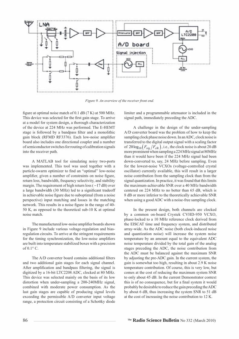
The two primary active subsystems in the Demonstrator receiver front end are the low-noise amplifi er (LNA) and the dual-channel A/D converter board. One antenna polarization is served by one low-noise amplifi er and half of one A/D converter board. An overview of the receiver chain is shown in Figure 9. All control signals and switches in the receiver electronics are connected to a microcontroller. This gives the possibility of controlling power-supply outputs, the coupler modes for signal injection, signal-injection frequency, low-noise amplifi ers, A/D converter boards, and temperature stabilization of the low-noise amplifi er boxes.

The target requirements for the low-noise amplifi er were:

• A bandwidth of 30 MHz

• A system noise temperature of 50 K

• A spurious-free dynamic range of 70 dB

• A return loss of 17 dB.

The applications for very-low-noise-fi gure (NF) amplifi ers operating at VHF frequencies are limited, and so is the number of available semiconductor devices. The device with the best specifi ed performance at a frequency not too different from the intended frequency range was the ATF-541M4 E-HEMT from Avago, with a specifi ed noise

Figure 8. The electron density, electron and ion tem-peratures, and ion drift velocity at 290 km altitude above Tromsø, derived from 224 MHz incoherent-scatter signals received by the Demonstrator array

on November 2, 2007. The signal-to-noise ratio dur-ing this observation varied between 4% and 6 %.


fi gure at optimal noise match of 0.1 dB (7 K) at 500 MHz. This device was selected for the fi rst gain stage. To arrive at a model for system design, a thorough characterization of the device at 224 MHz was performed. The E-HEMT stage is followed by a bandpass fi lter and a monolithic gain block (RFMD RF3376). Each low-noise amplifi er board also includes one directional coupler and a number of semiconductor switches for routing of calibration signals into the receiver path.

A MATLAB tool for simulating noisy two-ports was implemented. This tool was used together with a particle-swarm optimizer to fi nd an “optimal” low-noise amplifi er, given a number of constraints on noise fi gure, return loss, bandwidth, frequency selectivity, and stability margin. The requirement of high return loss ( 17 dB) over a large bandwidth (30 MHz) led to a signifi cant tradeoff in achievable noise fi gure due to suboptimal (from a noise perspective) input matching and losses in the matching network. This results in a noise fi gure in the range of 40-50 K, as opposed to the theoretical sub-10 K at optimal noise match.

The manufactured low-noise amplifi er boards shown in Figure 9 include various voltage-regulation and bias-regulation circuits. To arrive at the stringent requirements for the timing synchronization, the low-noise amplifi ers are built into temperature stabilized boxes with a precision of 0.1° C.

The A/D converter board contains additional fi lters and two additional gain stages for each signal channel. After amplifi cation and bandpass fi ltering, the signal is digitized by a 16-bit LTC2208 ADC, clocked at 80 MHz. This device was selected mainly on the basis of its low distortion when under-sampling a 200-240MHz signal, combined with moderate power consumption. As the last gain stages are capable of producing signal levels exceeding the permissible A/D converter input voltage range, a protection circuit consisting of a Schottky diode

limiter and a programmable attenuator is included in the signal path, immediately preceding the ADC.

A challenge in the design of the under-sampling A/D converter board was the problem of how to keep the sampling clock phase noise down. In an ADC, clock noise is transferred to the digital output signal with a scaling factor of 1020log sig clkF F , i.e., the clock noise is about 20 dB more prominent when sampling a 224 MHz signal at 80MHz than it would have been if the 224 MHz signal had been down-converted to, say, 24 MHz before sampling. Even for the lowest-noise VCXOs (voltage-controlled crystal oscillator) currently available, this will result in a larger noise contribution from the sampling clock than from the signal quantization. In practice, it was found that this limits the maximum-achievable SNR over a 40 MHz bandwidth centered on 224 MHz to no better than 65 dB, which is 8 dB or more inferior to the theoretically achievable SNR when using a good ADC with a noise-free sampling clock.

In the present design, both channels are clocked by a common on-board Crystek CVHD-950 VCXO, phase-locked to a 10 MHz reference clock derived from the EISCAT time and frequency system, and distributed array-wide. As the ADC noise (both clock-induced noise and quantization noise) will increase the system noise temperature by an amount equal to the equivalent ADC noise temperature divided by the total gain of the analog stages preceding the ADC, the noise contribution from the ADC must be balanced against the maximum SNR by adjusting the pre-ADC gain. In the current system, the gain is somewhat too high, resulting in about 2.9 K noise temperature contribution. Of course, this is very low, but comes at the cost of reducing the maximum system SNR to only about 45 dB. In the current Demonstrator context this is of no consequence, but for a fi nal system it would probably be desirable to reduce the gain preceding the ADC by about 6 dB, thus increasing the system SNR to 51 dB at the cost of increasing the noise contribution to 12 K.

Figure 9. An overview of the receiver front end.


11. Antenna Measurement System

Antennas operating in an Arctic environment may have their performance degraded signifi cantly due to snow and hoarfrost sticking to the antennas. This has been shown to be a problem affecting both the impedance of the antenna elements in an array [16], and the beam shape and pointing direction of large telescopes [17]. In the EISCAT_3D system, it is particularly important to assess the climatic effects, since the shape and pointing direction of the main beam must be quantitatively known.

The performance of the element antennas used in the Demonstrator array during snowfall has been studied [18]. The return loss, 11S , was measured continuously during a 48-hour period with signifi cant precipitation in the form of a snow/rain mixture. At the onset of the snowfall, the whole pass band of the antenna is shifted downwards and the bandwidth was reduced. On some occasions, the useable pass band of the antenna fell entirely outside the desired frequency band. This behavior agreed with results from simulations of a crossed Yagi antenna covered with a dielectric medium.

Simulations have also shown that there can be signifi cant distortion of both the amplitude and the phase of the far-fi eld pattern. Due to the stringent requirements of the relative timing between elements in the array, even a small shift in the far-fi eld phase could cause unacceptable errors in the beamforming process.

A popular technique for mitigating the effects of climate on large antennas is to place the whole antenna inside a radome. However, this is not practical in the EISCAT_3D case, due to the sheer physical size of the antenna arrays. For the same reason, deicing by heating the antennas is not a realistic option. A possible partial solution is to place only the driven elements of the crossed Yagi antennas inside a radome. The drawback is that the gain of the antennas would be reduced during snowfall. Ideally, the antennas should also be designed with a larger bandwidth than needed in order to be able to handle both the shift in frequency and the narrowing of the band. That this is possible is evidenced by, e.g., the results obtained in controlled tests of the “Renkwitz Yagi,” proposed as the element antenna for the core array [19]. A good compromise would likely include both of the solutions mentioned above.

The phase and amplitude of the far-fi eld pattern during snowfall are more diffi cult to control, and should therefore ideally be monitored. When the system is in actual operation, this can probably best be done by a near-fi eld measurement system, such as, e.g., the one presented in [20]. This system used probes located in the near fi eld of the antenna array to estimate the electric-current distribution on the antenna elements. The electric-current distribution can then be transformed into a complex far-fi eld pattern. The

technique has the advantage of using relatively few probes that can be located at varying distances from the antenna elements, which is necessary in an antenna array of the size considered here. Also, the whole far-fi eld pattern can be estimated without having probes in the main beam of the antenna, which minimizes the interference and diffraction effects that could degrade the performance of the radar.

12. Summary and Next Steps

In this paper, we have presented the results of an EU-funded study conducted into the design of the EISCAT_3D system, a next-generation incoherent-scatter radar to be deployed for atmospheric and geospace studies in the Scandinavian Arctic. As well as describing the novel elements in this new multi-static phased-array radar, we have drawn attention to some of the new scientifi c areas that the new facility will open up to its users, and outlined the principles under which it will operate (essentially continuous operation with un-staffed remote sites). While the concepts behind the design have been fi rmly established, some important details at the hardware level have still not been fi nally specifi ed, because of the speed at which cheaper and more effective signal-processing solutions are currently emerging. The fi nal choice of hardware in this area will only be made closer to the time of system construction.

The design study the results of which were presented here is only the fi rst of three development phases that will lead to the eventual realization of EISCAT_3D. In December 2008, the project was added to the ESFRI European roadmap for research infrastructures [21], which identifi es future programs and facilities corresponding to the long-term needs of the European research community. Acceptance into the roadmap is seen as an important recognition of the EISCAT_3D concept, which will lead to further opportunities to take the project forward within the context of future EU Framework Programmes.

It should be noted that although the design exercise reported here has produced a specifi cation for a radar facility with one active central site and four passive remote receivers, the fi nally constructed system may have a very different confi guration. Given the availability of suffi cient funding, it would be simple to scale up from the present design into a system with multiple active sites, offering unparalleled coverage of the upper atmosphere and geospace region above northern Scandinavia, and providing an unprecedentedly detailed data set to scientists in this important research area.

The next phase of EISCAT_3D development is likely to be a three-year preparatory study, hopefully beginning early in 2010, again using EU funding (this time under the Seventh Framework). In this phase, some remaining technical issues, including the choice of DSP and beam-forming hardware, will be fi nalized; frequency clearances will be confi rmed; site-selection issues will be resolved and construction permissions obtained; manufacturing


questions relating to the mass-production of thousands of antennas, transmitters, and signal-processing units will be clarifi ed; and a consortium will be established to fund the construction phase. It is anticipated that construction will begin around 2013, with fi rst operations around 2015. This will provide a state-of-the-art research radar with a nominal operating lifetime of 30 years, to yield top-quality data for the next generation of researchers in upper-atmospheric physics and geospace science.

13. Acknowledgements

The authors gratefully acknowledge the fi nancial support of the EU under its Sixth Framework Programme, which made this study possible. Financial and staffi ng commitments from each of the fi ve participating institutes, and the assistance of IAP Kühlungsborn and the University of Rostock in the antenna-design exercise, are also gratefully acknowledged.

14. References

1. EISCAT_3D Design Study Team, “EISCAT_3D: The Next Generation European Incoherent Scatter Radar, Final Design Study Report (D11.1),” available at http://e7.eiscat.se/groups/EISCAT_3D_info.

2. C. Ackerman, C. Miller, and J. Brown, “Theoretical Basis and Practical Implications of Band-Pass Sampling,” Proceedings of the National Electronics Conference, 18, 1962, pp. 1-9

3. T. Grydeland, C. la Hoz, T. Hagfors, E. M. Blixt, S. Saito, A. Strømme and A. Brekke, “Interferometric Observations of Filamentary Structures Associated with Plasma Instability in the Auroral Ionosphere,” Geophysical Research Letters, 30, 2003, pp. 1338-1348 (doi:10.1029/2002-GL016362).

4. T. Cornwell, “Deconvolution,” in G. B. Taylor, C. L. Carilli, and R. A. Perley (eds.), Synthesis Imaging in Radio Astronomy II, (ASP Conference Series, 180, xxxiii, 1999, ISBN No. 1583810056), pp. 167-184.

5. D. L. Hysell and J. L. Chau, “Optimal Aperture Syn-thesis Radar Imaging,” Radio Science, 41, 2006, (doi: 10.1029/2005RS003383).

6. P. Comon and G. H. Golub, “Tracking a Few Extreme Singular Values and Vectors in Signal Processing,” Proceedings of the IEEE, 78, 8, August 1990, pp. 1327-1343.

7. B. Yang, “Projection Approximation for Subspace Tracking,” IEEE Transactions on Signal Processing, 43, 1, 1995, pp. 95-107.

8. R. Badeau, B. David, and G. Richard, “Fast Approximated Power Iteration Subspace Tracking,” IEEE Transactions on Signal Processing, 53, 8, August 2005, pp. 2931-2941.

9. X. Doukopoulos and G. V. Moustakides, “Fast and Stable Subspace Tracking,” IEEE Transactions on Signal Processing, 56, 4, April 2008, pp. 1452-1465.

10. H. Krim and M. Viberg, “Two Decades of Array Signal Processing Research: The Parametric Approach,” IEEE Signal Processing Magazine, 13, 4, April 1996, pp. 67-94.

11. P. Murphy, A. Krukowski, and A. Tarczynski, “An Effi cient Fractional Sample Delayer for Digital Beam Steering,” IEEE International Conference on Acoustics, Speech, and Signal Processing (Cat.No.97CB36052), 3, 1997, pp. 2245-2248.

12. V. Välimäki and T. Laakso, “Principles of Fractional Delay Filters,” Proceedings of the IEEE International Conference on Acoustics, Speech, and Signal Processing, 6, 2000, pp. 3870-3873.

13. G. Johansson, J. Borg, J. Johansson, M. Lundberg-Norden-vaad and G. Wannberg, “Simulation of Post-ADC Digital Beam-Forming for Large Aperture Array Radars,” Radio Science, 2010 (in press).

14. W. Grover, “A New Method for Clock Distribution,” IEEE Transactions on Circuits and Systems: I, Fundamental Theory and Applications, 41, 2, February 1994, pp. 149-160.

15. G. Stenberg, T. Lindgren and J. Johansson, “A Picosecond Accuracy Timing System Based on L1-Only GNSS Receiv-ers for a Large Aperture Array Radar,” Proceedings of the Twenty-fi rst International Technical Meeting of the Satellite Division of the Institute of Navigation: ION GNSS 2008, Institute of Navigation, 2008, pp. 112-116.

16. L. D. Poles, J. P. Kenney and E. Martin, “UHF Phased Array Measurements in Snow,” IEEE Antennas and Propagation Magazine, 46, 5, October 2004, pp. 181-184.

17. E. Salonen and P. Jokela, “The Effects of Dry Snow on Re-fl ector Antennas,” Proceedings of the Seventh International Conference on Antennas and Propagation, 1, 1991, pp. 17-20.

18. T. Lindgren, Characterization Problems in Radio Measure-ment Systems, Doctoral Thesis, Luleå University of Technol-ogy, Sweden, 2009, ISBN 978-91-7439-034-6.

19. EISCAT_3D Design Study Team, “EISCAT_3D: Options for the Active Element (D3.2),” available at http://e7.eiscat.se/groups/EISCAT_3D_info.

20. T. Lindgren and J. Ekman, “A Measurement System for the Complex Far-Field of Physically Large Antenna Arrays under Noisy Conditions Utilizing the Equivalent Electric Current Method,” submitted to IEEE Transactions on Antennas and Propagation, 2010.

21. ESFRI, European Strategy Forum on Research Infra-structures, Roadmap Update 2008, available at ftp://ftp.cordis.europa.eu/pub/esfri/docs/esfri_roadmap_2008_up-date_20090123.pdf.

Documents

EISCAT 3D: A Next-Generation European Radar … Radio Science Bulletin No 332 (March 2010) 75 EISCAT_3D: A Next-Generation European Radar System for Upper-Atmosphere and Geospace Research