Embed Size (px)
Citation preview

7/28/2019 Ek Econometric a 2002
http://slidepdf.com/reader/full/ek-econometric-a-2002 1/40
Technology, Geography, and TradeAuthor(s): Jonathan Eaton and Samuel KortumSource: Econometrica, Vol. 70, No. 5 (Sep., 2002), pp. 1741-1779Published by: The Econometric SocietyStable URL: http://www.jstor.org/stable/3082019
Accessed: 30/12/2008 09:53
Your use of the JSTOR archive indicates your acceptance of JSTOR's Terms and Conditions of Use, available at
http://www.jstor.org/page/info/about/policies/terms.jsp. JSTOR's Terms and Conditions of Use provides, in part, that unless
you have obtained prior permission, you may not download an entire issue of a journal or multiple copies of articles, and you
may use content in the JSTOR archive only for your personal, non-commercial use.
Please contact the publisher regarding any further use of this work. Publisher contact information may be obtained at
http://www.jstor.org/action/showPublisher?publisherCode=econosoc.
Each copy of any part of a JSTOR transmission must contain the same copyright notice that appears on the screen or printed
page of such transmission.
JSTOR is a not-for-profit organization founded in 1995 to build trusted digital archives for scholarship. We work with the
scholarly community to preserve their work and the materials they rely upon, and to build a common research platform that
promotes the discovery and use of these resources. For more information about JSTOR, please contact [email protected].
The Econometric Society is collaborating with JSTOR to digitize, preserve and extend access to Econometrica.
http://www.jstor.org

7/28/2019 Ek Econometric a 2002
http://slidepdf.com/reader/full/ek-econometric-a-2002 2/40
Econometrica, Vol. 70, No. 5 (September, 2002), 1741-1779
TECHNOLOGY, GEOGRAPHY, AND TRADE
BY JONATHAN EATON AND SAMUEL KORTUM1
We develop a Ricardian trade model that incorporates realistic geographic features
into general equilibrium. It delivers simple structural equations for bilateral trade with
parameters relating to absolute advantage, to comparative advantage (promoting trade),
and to geographic barriers (resisting it). We estimate the parameters with data on bilateral
trade in manufactures, prices, and geography from 19 OECD countries in 1990. We use the
model to explore various issues such as the gains from trade, the role of trade in spreading
the benefits of new technology, and the effects of tariff reduction.
KEYWORDS: Trade, gravity, technology, geography, research, integration, bilateral.
1. INTRODUCTION
THEORIES OF INTERNATIONAL TRADE have not come to grips with a num-
ber of basic facts: (i) trade diminishes dramaticallywith distance; (ii) prices vary
across locations, with greater differences between places farther apart; (iii) factor
rewards are far from equal across countries; (iv) countries' relative productivitiesvary substantially across industries. The first pairof facts indicate that geography
plays an important role in economic activity.The second pair suggest that coun-
tries are working with different technologies. Various studies have confrontedthese features individually,but have not provided a simple framework that cap-tures all of them.
We develop and quantify a Ricardian model of international trade (one based
on differences in technology) that incorporates a role for geography.2The model
captures the competing forces of comparative advantagepromoting trade and of
geographic barriers (both natural and artificial) inhibiting it. These geographicbarriers reflect such myriad impediments as transport costs, tariffs and quotas,
delay, and problems with negotiating a deal from afar.
The model yields simple expressions relating bilateral trade volumes, first, to
deviations from purchasing power parity and, second, to technology and geo-graphic barriers.3 From these two relationships we can estimate the parameters
1 A previous version circulated under the title "Technology and Bilateral Trade," NBER Working
Paper No. 6253, November, 1997. Deepak Agrawal and Xiaokang Zhu provided excellent research
assistance. We gratefully acknowledge the helpful comments of Zvi Eckstein and two anonymous
referees as well as the support of the National Science Foundation.
2 Grossman and Helpman (1995) survey the literature on technology and trade while Krugman
(1991) provides an introduction to geography and trade.3 Engel and Rogers (1996) and Crucini, Telmer, and Zachariadis (2001) explore the geographic
determinants of deviations from the law of one price.
1741

7/28/2019 Ek Econometric a 2002
http://slidepdf.com/reader/full/ek-econometric-a-2002 3/40
1742 J. EATON AND S. KORTUM
needed to solve the world trading equilibrium of the model and to examine howit changes in response to various policies.
Our point of departure is the Dornbusch, Fischer, and Samuelson (1977) two-country Ricardian model with a continuum of goods. We employ a probabilisticformulation of technological heterogeneity under which the model extends nat-urally to a world with many countries separated by geographic barriers. Thisformulation leads to a tractable and flexible framework for incorporating geo-graphical features into general equilibrium analysis.
An additional feature of our model is that it can recognize, in a simple way,the preponderance of trade in intermediate products. Trade in intermediates hasimportant implications for the sensitivity of trade to factor costs and to geo-graphic barriers. Furthermore, because of intermediates, location, through itseffect on input cost, plays an important role in determining specialization.4
We estimate the model using bilateral trade in manufactures for a cross-sectionof 19 OECD countries in 1990.5The parameters correspond to: (i) each country'sstate of technology, governing absolute advantage, (ii) the heterogeneity of tech-nology, which governs comparative advantage, and (iii) geographic barriers. Wepursue several strategies to estimate these parameters using different structuralequations delivered by the model and data on trade flows, prices, geography, andwages.
Our parameter estimates allow us to quantify the general equilibrium of ourmodel in order to explore numerically a number of counterfactual situations:
(i) We explore the gains from trade in manufactures. Not surprisingly, all
countries benefit from freer world trade, with small countries gaining more thanbig ones. The cost of a move to autarky in manufactures is modest relative tothe gains from a move to a "zero gravity" world with no geographic barriers.
(ii) We examine how technology and geography determine patterns of special-ization. As geographic barriers fall from their autarky level, manufacturingshiftstoward larger countries where intermediate inputs tend to be cheaper. But atsome point further declines reverse this pattern as smaller countries can also buyintermediates cheaply. A decline in geographic barriers from their current leveltends to work against the largest countries and favor the smallest.(iii) We calculate the role of trade in spreading the benefits of new technology.
An improvement in a country's state of technology raises welfare almost every-where. But the magnitude of the gains abroad approach those at home only incountries enjoying proximityto the source and the flexibility to downsize manu-facturing.
4Hummels, Rapoport, and Yi (1998) document the importance of trade in intermediates. Yi(forthcoming) discusses how trade in intermediates, which implies that a good might cross bordersseveral times during its production, can reconcile the large rise in world trade with relatively modest
tariff reductions. Krugman and Venables (1995) also provide a model in which, because of trade inintermediates, geography influences the location of industry.
5 We think that our model best describes trade in manufactures among industrial countries. Formost of these countries trade in manufactures represents over 75 percent of total merchandise trade.
(The exceptions are Australian exports and Japanese imports.) Moreover, the countries in our sampletrade mostly with each other, as shown in the second column of Table I.

7/28/2019 Ek Econometric a 2002
http://slidepdf.com/reader/full/ek-econometric-a-2002 4/40
TECHNOLOGY, GEOGRAPHY, AND TRADE 1743
TABLE I
TRADE,LABOR, AND INCOME DATA
Imports Imports from Sample as Human-Capital Adj.
% of Mfg. % of Mfg. Wage Mfg. Wage Mfg. Labor Mfg. Labor's
Country Spending All Imports (U.S. = 1) (U.S. = 1) (U.S. = 1) % Share of GDP
Australia 23.8 75.8 0.61 0.75 0.050 8.6
Austria 40.4 84.2 0.70 0.87 0.036 13.4
Belgium 74.8 86.7 0.92 1.08 0.035 13.2
Canada 37.3 89.6 0.88 0.99 0.087 10.5
Denmark 50.8 85.2 0.80 1.10 0.020 11.5
Finland 31.3 82.2 1.02 1.10 0.022 12.5
France 29.6 82.3 0.92 1.07 0.205 12.6
Germany 25.0 77.3 0.97 1.08 0.421 20.6
Greece 42.9 80.8 0.40 0.50 0.015 6.1
Italy 21.3 76.8 0.74 0.88 0.225 12.4
Japan 6.4 50.0 0.78 0.91 0.686 14.4
Netherlands 66.9 83.0 0.91 1.06 0.043 11.0
New Zealand 36.3 80.9 0.48 0.57 0.011 9.6
Norway 43.6 85.2 0.99 1.18 0.012 8.7
Portugal 41.6 84.9 0.23 0.32 0.033 10.7
Spain 24.5 82.0 0.56 0.65 0.128 11.6
Sweden 37.3 86.3 0.96 1.11 0.043 14.2
United Kingdom 31.3 79.1 0.73 0.91 0.232 14.7
United States 14.5 62.0 1.00 1.00 1.000 12.4
Notes: All data except GDP are for the manufacturing sector in 1990. Spending on manufactures is gross manufacturingproduction less exports of manufactures plus imports of manufactures. Imports from the other 18 excludes imports of manufactures
from outside our sample of countries. To adjust the manufacturing wage and manufacturing employment for human capital, wemultiply the wage in country i by e-0.06Hi and employment in country i by eO0O6Hi,here Hi is average years of schooling incountry i as measured by Kyriacou (1991). See the Appendix for a complete description of all data sources.
(iv) We analyze the consequences of tariff reductions. Nearly every countrybenefits from a multilateral move to freer trade, but the United States suffers ifit drops its tariffs unilaterally. Depending on internal labor mobility, Europeanregional integration has the potential to harm participants through trade diver-
sion or to harm nonparticipants nearby through worsened terms of trade.With a handful of exceptions, the Ricardian model has not previously served as
the basis for the empirical analysis of trade flows, probablybecause its standard
formulation glosses over so many first-order features of the data (e.g., multiplecountries and goods, trade in intermediates, and geographic barriers).6 Moreactive empirical fronts have been: (i) the gravitymodeling of bilateral trade flows,(ii) computable general equilibrium (CGE) models of the international economy,and (iii) factor endowments or Heckscher-Ohlin-Vanek (HOV) explanations of
trade.Our theory implies that bilateral trade volumes adhere to a structure resem-
bling a gravity equation, which relates trade flows to distance and to the product
6 What has been done typically compares the export performance of only a pair of countries.
MacDougall (1951, 1952) is the classic reference. Deardorff (1984) and Leamer and Levinsohn
(1995) discuss it and the subsequent literature. Choudhri and Schembri (forthcoming) make a recentcontribution.

7/28/2019 Ek Econometric a 2002
http://slidepdf.com/reader/full/ek-econometric-a-2002 5/40
1744 J. EATON AND S. KORTUM
of the source and destination countries' GDPs. Given the success of the gravitymodel in explaining the data, this feature of our model is an empirical plus.7 But
to perform counterfactuals we must scratch beneath the surface of the gravityequation to uncover the structuralparameters governing the roles of technologyand geography in trade.8
In common with CGE models we analyze trade flows within a general equi-
librium framework, so we can conduct policy experiments. Our specification ismore Spartan than a typical CGE model, however. For one thing, CGE models
usually treat each country's goods as unique, entering preferences separately asin Armington (1969).9 In contrast, we take the Ricardian approach of definingthe set of commodities independent of country, with specialization governed bycomparative advantage.
Our approach has less in common with the empirical work emanating from theHOV model, which has focussed on the relationship between factor endowmentsand patterns of specialization. This work has tended to ignore locational ques-tions (by treating trade as costless), technology (by assuming that it is common
to the world), and bilateral trade volumes (since the model makes no predictionabout them).10 While we make the Ricardian assumption that labor is the onlyinternationally immobile factor, in principle one could bridge the two approaches
by incorporating additional immobile factors.To focus immediately on the most novel features of the model and how they
relate to the data we present our analysis in a somewhat nonstandard order.
Section 2, which follows, sets out our model of trade, conditioning on input costsaround the world. It delivers relationships connecting bilateral trade flows to
prices as well as to geographic barriers, technology, and input costs. We explore
empirically the trade-price relationship in Section 3. In Section 4 we completethe theory, closing the model to determine input costs. With the full model in
hand, Section 5 follows several approaches to estimating its parameters. Section 6
7Deardorff (1984) reviews the earlier gravity literature. For recent applications see Wei (1996),Jensen (2000), Rauch (1999), Helpman (1987), Hummels and Levinsohn (1995), and Evenett and
Keller (2002).
8 We are certainly not the first to give the gravity equation a structural interpretation. Previous
theoretical justifications posit that every country specializes in a unique set of goods, either by mak-ing the Armington assumption (as in Anderson (1979) and Anderson and van Wincoop (2001)) or
by assuming monopolistic competition with firms in different countries choosing to produce differ-
entiated products (as in Helpman (1987), Bergstrand (1989), and Redding and Venables (2001)). An
implication is that each source should export a specific good everywhere. Haveman and Hummels
(2002) report evidence to the contrary. In our model more than one country may produce the same
good, with individual countries supplying different parts of the world.9 Hertel (1997) is a recent state-of-the-art example.
10Leamer (1984) epitomizes this approach, although Leamer and Levinsohn (1995) admit its fail-
ure to deal with the obvious role of geographic barriers. The literature has begun to incorporate rolesfor technology, introducing factor-augmenting technological differences, as in Trefler (1993, 1995)and industry-specifictechnological differences, as in Harrigan (1997). Trefler (1995) recognizes geog-
raphy by incorporating a home-bias in preferences. Davis and Weinstein (2001) strive to incorporatemore general geographic features.
7/28/2019 Ek Econometric a 2002
http://slidepdf.com/reader/full/ek-econometric-a-2002 6/40
TECHNOLOGY, GEOGRAPHY, AND TRADE 1745
uses the quantified model to explore the counterfactual scenarios listed above.
Section 7 concludes. (The Appendix reports data details.)
2. A MODEL OF TECHNOLOGY, PRICES, AND TRADE FLOWS
We build on the Dornbusch, Fischer, Samuelson (1977) model of Ricardian
trade with a continuum of goods. As in Ricardo, countries have differential accessto technology, so that efficiency varies across commodities and countries. Wedenote country i's efficiency in producing good j E [0, 1] as zi(j).
Also as in Ricardo, we treat the cost of a bundle of inputs as the same acrosscommodities within a country (because within a country inputs are mobile acrossactivities and because activities do not differ in their input shares). We denote
input cost in country i as ci. With constant returns to scale, the cost of producinga unit of good j in country i is then ci/zi(j).
Later we break ci into the cost of labor and of intermediate inputs, model how
they are determined, and assign a numeraire. For now it suffices to take as given
the entire vector of costs across countries.We introduce geographic barriers by making Samuelson's standard and con-
venient "iceberg" assumption, that delivering a unit from country i to country n
requires producing dniunits in i.11We set dii = 1 for all i. Positive geographic
barriers mean dni> 1 for n 0 i. We assume that cross-border arbitrage forces
effective geographic barriersto obey the triangle inequality: For any three coun-
tries i, k, and n, dni < dnkdki.Taking these barriers into account, delivering a unit of good j produced in
country i to country n costs
(1) Pni()= ( )dni
the unit production cost multiplied by the geographic barrier.
We assume perfect competition, so that pni(i) is what buyers in country n
would pay if they chose to buy good j from country i. But shopping around the
world for the best deal, the price they actually pay for good j will be pn(), the
lowest across all sources i:
(2) Pn ) = minbPnir; 1ountr i,
where N is the number of countries.12
11Krugman (1995) extols the virtues of this assumption. Most relevant here is that country i's
relative cost of supplying any two goods does not depend on the destination.
12 Bernard, Eaton, Jensen, and Kortum (2000) extend the analysis to allow for imperfect competi-
tion to explain why exporting plants have higher productivity, as documented in Bernard and Jensen
(1999). With Bertrand competition each destination is still served by the low-cost provider, but it
charges the cost of the second-cheapest potential provider. The implications for the aggregate rela-tionships we examine below are not affected.

7/28/2019 Ek Econometric a 2002
http://slidepdf.com/reader/full/ek-econometric-a-2002 7/40
1746 J. EATON AND S. KORTUM
Facing these prices, buyers (who could be final consumers or firms buyingintermediate inputs) purchase individual goods in amounts Q(j) to maximize a
CES objective:
(3) U= Q(i)(1')'ad i]j
where the elasticity of substitution is u-> 0. This maximization is subject to abudget constraint that aggregates, across buyers in country n, to Xn, country n's
total spending.Dornbusch, Fischer, and Samuelson work out the two-country case, but their
approach does not generalize to more countries.13 Extending the model beyond
this case is not only of theoretical interest, it is essential to any empirical analysis
of bilateral trade flows.
2.1. Technology
We pursue a probabilistic representation of technologies that can relate tradeflows to underlying parameters for an arbitrary number of countries across ourcontinuum of goods. We assume that country i's efficiency in producing good
j is the realization of a random variable Zi (drawn independently for each j)from its country-specific probabilitydistribution Fi(z) = Pr[Zi < z]. We follow theconvention that, by the law of large numbers, Fi z) is also the fraction of goods
for which country i's efficiency is below z.From expression (1) the cost of purchasing a particular good from country i in
country n is the realization of the random variable Pni= cidnilZi and from (2)the lowest price is the realization of Pn= min{Pni;i = 1, .. , N}. The likelihoodthat country i supplies a particular good to country n is the probability Tnithati's price turns out to be the lowest.
The probability theory of extremes provides a form for Fi(z) that yields a
simple expression for 7ni and for the resulting distribution of prices. We assumethat country i's efficiency distribution is Frechet (also called the Type II extremevalue distribution):
(4) Fi(z) = e-Tiz-0
where Ti> 0 and 0 > 1. We treat the distributions as independent across coun-
tries. The (country-specific) parameter Tigoverns the location of the distribution.
13 For two countries 1 and 2 they order commodities j according to the countries' relative effi-
ciencies z1(])/z2(j). Relative wages (determined by demand and labor supplies) then determine the
breakpoint in this "chain of comparative advantage." With more than two countries there is no such
natural ordering of commodities. Wilson (1980) shows how to conduct local comparative static exer-
cises for the N-country case by asserting that zi(j) is a continuous function of j. Closer to our
probabilistic formulation, although with a finite number of goods and no geographic barriers, is Petri
(1980). Neither paper relates trade flows or prices to underlying parameters of technology or geo-graphic barriers, as we do here.
7/28/2019 Ek Econometric a 2002
http://slidepdf.com/reader/full/ek-econometric-a-2002 8/40
TECHNOLOGY, GEOGRAPHY, AND TRADE 1747
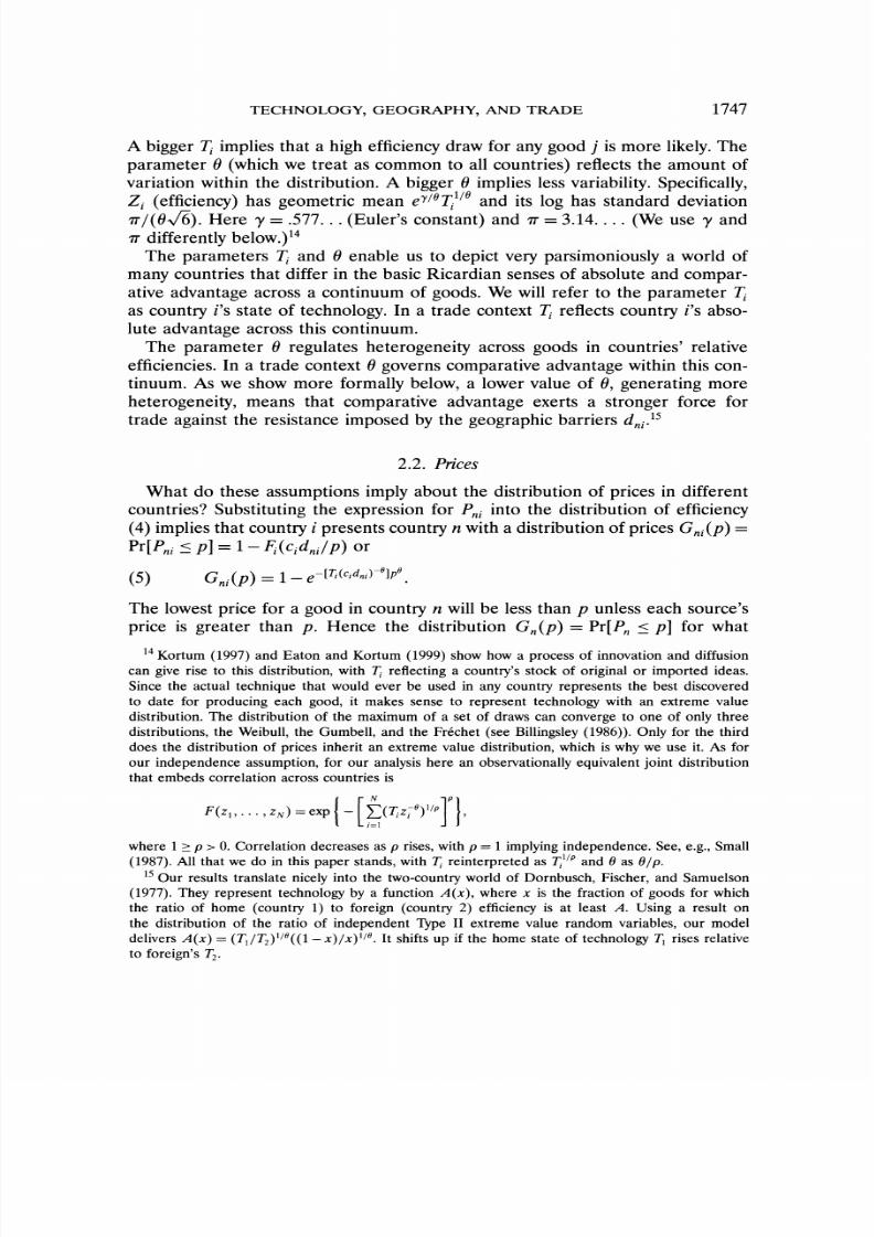
A bigger Ti implies that a high efficiency draw for any good j is more likely. Theparameter 0 (which we treat as common to all countries) reflects the amount of
variation within the distribution. A bigger 0 implies less variability. Specifically,Z. (efficiency) has geometric mean el0lTillo and its log has standard deviation
7r/(06V). Here ry= .577... (Euler's constant) and 7T= 3.14.... (We use ryand7Tdifferently below.)"4
The parameters Ti and 0 enable us to depict very parsimoniously a world ofmany countries that differ in the basic Ricardian senses of absolute and compar-ative advantage across a continuum of goods. We will refer to the parameter Tias country i's state of technology. In a trade context Ti reflects country i's abso-lute advantage across this continuum.
The parameter 0 regulates heterogeneity across goods in countries' relative
efficiencies. In a trade context 0 governs comparative advantagewithin this con-tinuum. As we show more formally below, a lower value of 0, generating moreheterogeneity, means that comparative advantage exerts a stronger force fortrade against the resistance imposed by the geographic barriers d i.15
2.2. Prices
What do these assumptions imply about the distribution of prices in differentcountries? Substituting the expression for Pniinto the distribution of efficiency(4) implies that country i presents country n with a distribution of prices Gni(p) =
Pr[Pni< p] = 1 - Fi(cidni/p) or
(5) Gni(p) = 1 - e-[(cidni)6]p0
The lowest price for a good in country n will be less than p unless each source'sprice is greater than p. Hence the distribution Gj(p) = Pr[Pn < p] for what
14 Kortum (1997) and Eaton and Kortum (1999) show how a process of innovation and diffusion
can give rise to this distribution, with Ti reflecting a country's stock of original or imported ideas.
Since the actual technique that would ever be used in any country represents the best discovered
to date for producing each good, it makes sense to represent technology with an extreme value
distribution. The distribution of the maximum of a set of draws can converge to one of only three
distributions, the Weibull, the Gumbell, and the Frechet (see Billingsley (1986)). Only for the third
does the distribution of prices inherit an extreme value distribution, which is why we use it. As forour independence assumption, for our analysis here an observationally equivalent joint distribution
that embeds correlation across countries is
F(zl,...,ZN) = exp ( [E(Tiz0)1/]P1
where 1 > p > 0. Correlation decreases as p rises, with p = 1 implying independence. See, e.g., Small
(1987). All that we do in this paper stands, with Ti reinterpreted as Tillpand 0 as 6/p.15 Our results translate nicely into the two-country world of Dornbusch, Fischer, and Samuelson
(1977). They represent technology by a function A(x), where x is the fraction of goods for which
the ratio of home (country 1) to foreign (country 2) efficiency is at least A. Using a result on
the distribution of the ratio of independent Type II extreme value random variables, our model
delivers A(x) = (Tl/T2)I/0((1 - x)/x)"0. It shifts up if the home state of technology T1rises relative
to foreign's T2.

7/28/2019 Ek Econometric a 2002
http://slidepdf.com/reader/full/ek-econometric-a-2002 9/40
1748 J. EATON AND S. KORTUM
country n actually buys is
N
Gn(p) = 1- l[l-Gni(P)]i=1
Inserting (5), the price distribution inherits the form of Gni(p):
(6) Gn(p) = 1-e-"po
where the parameter On of country n's price distribution is
N
(7) = Tii=l
The price parameter On is critical to what follows. It summarizes how (i)states of technology around the world, (ii) input costs around the world, and (iii)
geographic barriers govern prices in each country n. International trade enlarges
each country's effective state of technology with technology available from other
countries, discounted by input costs and geographic barriers. At one extreme, in
a zero-gravity world with no geographic barriers (dni = 1 for all n and i), ' is
the same everywhere and the law of one price holds for each good. At the other
extreme of autarky,with prohibitive geographic barriers (dni -x oc for n 0 i), Onreduces to Tnc-j, country n's own state of technology downweighted by its input
cost.
We exploit three useful properties of the price distributions:(a) The probabilitythat country i provides a good at the lowest price in country
n is simply
(8) _ni = __(c_dni_ XOIn
i's contribution to country n's price parameter.16Since there are a continuum
of goods, this probability is also the fraction of goods that country n buys from
country i.(b) The price of a good that country n actually buys from any country i also
has the distribution Gn p).17 Thus, for goods that are purchased, conditioningon the source has no bearing on the good's price. A source with a higher state of
technology, lower input cost, or lower barriers exploits its advantage by selling a
wider range of goods, exactly to the point at which the distribution of prices for
what it sells in n is the same as n's overall price distribution.
16We obtain this probability by calculating
ITni=Pr[Pni(i) < min{Pns(i); s 7 i}]= l[l - Gns(p)] dGni(P).s$i
17We obtain this result by showing that
Gn P)==-,/; H[1-Gns (q)] dGni(q).I7T, J,so

7/28/2019 Ek Econometric a 2002
http://slidepdf.com/reader/full/ek-econometric-a-2002 10/40
TECHNOLOGY, GEOGRAPHY, AND TRADE 1749
(c) The exact price index for the CES objective function (3), assuming o- <
1+0, is
(9) Pn n
Here
where F is the Gamma function.18 This expression for the price index showshow geographic barriers,by generating different values of the price parameter in
different countries, lead to deviations from purchasing power parity.
2.3. TradeFlows, and Gravity
To link the model to data on trade shares we exploit an immediate corollaryof Property (b), that country n's average expenditure per good does not vary bysource. Hence the fraction of goods that country n buys from country i, 7nifrom
Property (a), is also the fraction of its expenditureon goods from country i:
Xni Ti(cidni) Ticidni)_-H
(10) -XOn k=1 Tk(Ckdnk)o'
where Xn is country n's total spending, of which Xni is spent (c.i.f.) on goods
from i.19Before proceeding with our own analysis, we discuss how expression(10) relates to the existing literature on bilateral trade.
Note that expression (10) already bears semblance to the standard gravityequation in that bilateral trade is related to the importer's total expenditureand to geographic barriers. Some manipulation brings it even closer to a gravityexpression. Note that the exporter's total sales Qi are simply
N N d,-X
Qi =E Xmi=IC 0E mi mm=1 m=1 m
18 The moment generating function for x = - lnp is E(etx) = c5/F(1 - t/0). (See, e.g., Johnson
and Kotz (1970).) Hence E[p-t]-1lt = F(1 - t/O)-"1t 5-1/1.The result follows by replacing t with a -1.
While our framework allows for the possibility of inelastic demand (cr< 1), we must restrict cr < 1+ 0
in order to have a well defined price index. As long as this restriction is satisfied, the parameter a can
be ignored, since it appears only in the constant term (common across countries) of the price index.
19Our model of trade bears resemblance to discrete-choice models of market share, popular in
industrial organization (e.g., McFadden (1974), Anderson, dePalma, and Thisse (1992), and Berry
(1994)): (i) Our trade model has a discrete number of countries whereas their consumer demand
model has a discrete number of differentiated goods; (ii) in our model a good's efficiency of produc-
tion in different countries is distributed multivariate extreme value whereas in their's a consumer's
preferences for different goods is distributed multivariateextreme value; (iii) in our model each good
is purchased (by a given importing country) from only one exporting country whereas in their model
each consumer purchases only one good; (iv) we assume a continuum of goods whereas they assume
a continuum of consumers. A distinction is that we can derive the extreme value distribution fromdeeper assumptions about the process of innovation.

7/28/2019 Ek Econometric a 2002
http://slidepdf.com/reader/full/ek-econometric-a-2002 11/40
1750 J. EATON AND S. KORTUM
Solving for TIcj0, and substituting it into (10), incorporating (9), we get
(ll) Xni = N (d i)-69XMQEm=l Pmm
Here, as in the standard gravityequation, both the exporter's total sales Qi and,given the denominator, the importer's total purchases Xn enter with unit elastic-
ity. Note that the geographic barrier dmibetween i and any importerm is deflated
by the importer's price level pm: Stiffer competition in market m reduces Pm,reducing i's access in the same way as a higher geographic barrier.We can thusthink of the term (dmi/pm)-0Xm as the market size of destination m as perceivedby country i. The denominator of the right-hand side of (11), then, is the total
world market from country i's perspective. The share of country n in country i'stotal sales just equals n's share of i's effective world market.Other justifications for a gravity equation have rested on the traditional
Armington and monopolistic competition models. Under the Armington assump-tion goods produced by different sources are inherently imperfect substitutes byvirtue of their provenance. Under monopolistic competition each country chooses
to specialize in a distinct set of goods. The more substitutable are goods fromdifferent countries, the higher is the sensitivity of trade to production costs and
geographic barriers. In contrast, in our model the sensitivity of trade to costsand geographic barriers depends on the technological parameter 0 (reflecting theheterogeneity of goods in production) rather than the preference parameter cr(reflecting the heterogeneity of goods in consumption). Trade shares respond tocosts and geographic barriers at the extensive margin:As a source becomes more
expensive or remote it exports a narrowerrange of goods. In contrast, in modelsthat invoke Armington or (with some caveats) monopolistic competition, adjust-ment is at the intensive margin:Higher costs or geographic barriers leave the setof goods that are traded unaffected, but less is spent on each imported good.20
20The expressions for bilateral trade shares delivered by the Armington and monopolistic compe-
tition models make the connections among these approaches explicit. For the Armington case define
ai as the weight on goods from country i in CES preferences. Country i's share in country n's expen-
diture is then
Xni aiJ I( dni) (J1
Xn EN I a''(Ckdnk)-(0f-l)
In the case of monopolistic competition with CES preferences define mi as the number of goods
produced by country i. Country i's share in country n's expenditure is then
Xni mi(cidni)('J )
Xn _k==Mk (Ckdnk)
Returning to equation (10), the exporter's state of technology parameter Ti in our model replaces its
preference weight ao'-' (in Armington) or its number of goods mi (under monopolistic competition).
In our model the heterogeneity of technology parameter 0 replaces the preference parameter r 1
in these alternatives. (The standard assumption in these other models is that all goods are producedwith the same efficiency, so that ci reflects both the cost of inputs and the f.o.b. price of goods.)
7/28/2019 Ek Econometric a 2002
http://slidepdf.com/reader/full/ek-econometric-a-2002 12/40
TECHNOLOGY, GEOGRAPHY, AND TRADE 1751
3. TRADE, GEOGRAPHY, AND PRICES: A FIRST LOOK
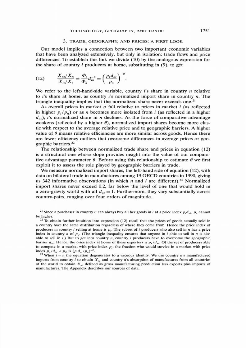
Our model implies a connection between two important economic variablesthat have been analyzed extensively, but only in isolation: trade flows and pricedifferences. To establish this link we divide (10) by the analogous expression forthe share of country i producers at home, substituting in (9), to get
(12) Xni=lX Ld-H pidni)
We refer to the left-hand-side variable, country i's share in country n relativeto i's share at home, as country i's normalized import share in country n. The
triangle inequality implies that the normalized share never exceeds one.21
As overall prices in market n fall relative to prices in market i (as reflectedin higher Pi/PM)or as n becomes more isolated from i (as reflected in a higher
dni), i's normalized share in n declines. As the force of comparative advantageweakens (reflected by a higher 0), normalized import shares become more elas-tic with respect to the average relative price and to geographic barriers.A higher
value of 0 means relative efficiencies are more similar across goods. Hence thereare fewer efficiency outliers that overcome differences in average prices or geo-graphic barriers.22
The relationship between normalized trade share and prices in equation (12)is a structural one whose slope provides insight into the value of our compara-
tive advantage parameter 0. Before using this relationship to estimate 0 we first
exploit it to assess the role played by geographic barriers in trade.
We measure normalized import shares, the left-hand side of equation (12), withdata on bilateral trade in manufactures among 19 OECD countries in 1990, givingus 342 informative observations (in which n and i are different).23Normalized
import shares never exceed 0.2, far below the level of one that would hold in
a zero-gravityworld with all dni= 1. Furthermore, they vary substantially across
country-pairs, ranging over four orders of magnitude.
21Since a purchaser in country n can always buy all her goods in i at a price index pi dni, Pn cannot
be higher.22To obtain further intuition into expression (12) recall that the prices of goods actually sold in
a country have the same distribution regardless of where they come from. Hence the price index of
producers in country i selling at home is pi. The subset of i producers who also sell in n has a price
index in country n of Pn. (The triangle inequality ensures that anyone in i able to sell in n is also
able to sell in i.) But to get into country n, country i producers have to overcome the geographicbarrier dni. Hence, the price index at home of these exporters is Pnldni. Of the set of producers able
to compete in a market with price index pi, the fraction who would survive in a market with priceindex Pn/dni < Pi, is (pid/niPn)6.
23When i = n the equation degenerates to a vacuous identity. We use country n's manufactured
imports from country i to obtain Xni and country n's absorption of manufactures from all countries
of the world to obtain Xn, defined as gross manufacturing production less exports plus imports of
manufactures. The Appendix describes our sources of data.

7/28/2019 Ek Econometric a 2002
http://slidepdf.com/reader/full/ek-econometric-a-2002 13/40

7/28/2019 Ek Econometric a 2002
http://slidepdf.com/reader/full/ek-econometric-a-2002 14/40

7/28/2019 Ek Econometric a 2002
http://slidepdf.com/reader/full/ek-econometric-a-2002 15/40
1754 J. EATON AND S. KORTUM
TABLE II
PRICE MEASURE STATISTICS
Foreign Sources Foreign Destinations
Country Minimum Maximum Minimum Maximum
Australia (AL) NE (1.44) PO (2.25) BE (1.41) US (2.03)
Austria (AS) SW (1.39) NZ (2.16) UK (1.47) JP (1.97)
Belgium (BE) GE (1.25) JP (2.02) GE (1.35) SW (1.77)
Canada (CA) US (1.58) NZ (2.57) AS (1.57) US (2.14)
Denmark (DK) Fl (1.36) PO (2.21) NE (1.48) US (2.41)
Finland (FI) SW (1.38) PO (2.61) DK (1.36) US (2.87)
France (FR) GE (1.33) NZ (2.42) BE (1.40) JP (2.40)
Germany (GE) BE (1.35) NZ (2.28) BE (1.25) US (2.22)
Greece (GR) SP (1.61) NZ (2.71) NE (1.48) US (2.27)
Italy (IT) FR (1.45) NZ (2.19) AS (1.46) JP (2.10)Japan (JP) BE (1.62) PO (3.25) AL (1.72) US (3.08)
Netherlands (NE) GE (1.30) NZ (2.17) DK (1.39) NZ (2.01)
New Zealand (NZ) CA (1.60) PO (2.08) AL (1.64) GR (2.71)
Norway (NO) Fl (1.45) JP (2.84) SW (1.36) US (2.31)
Portugal (PO) BE (1.49) JP (2.56) SP (1.59) JP (3.25)
Spain (SP) BE (1.39) JP (2.47) NO (1.51) JP (3.05)
Sweden (SW) NO (1.36) US (2.70) FI (1.38) US (2.01)
United Kingdom (UK) NE (1.46) JP (2.37) FR (1.52) NZ (2.04)
United States (US) FR (1.57) JP (3.08) CA (1.58) SW (2.70)
Notes: The price measure Di is defined in equation (13). For destination country n, the minimum Foreign Source is
mini#n exp D,i. For source country i, the minimum Foreign Destination is minn7i exp Dni.
Figure 2 graphs our measure of normalized import share (in logarithms)against Dni. Observe that, while the scatter is fat, there is an obvious negativerelationship, as the theory predicts. The correlation is -0.40. The relationship in
Figure 2 thus confirms the connection between trade and prices predicted by ourmodel.
Moreover, the slope of the relationship provides a handle on the value of the
comparative advantage parameter 0. Since our theory implies a zero intercept,a simple method-of-moments estimator for 0 is the mean of the left-hand-sidevariable over the mean of the right-hand-side variable. The implied 0 is 8.28.Other appropriate estimation procedures yield very similar magnitudes.27Hence
27 A linear regression through the scatter in Figure 2 yields a slope of -4.57 with an intercept of
-2.17 (with respective standard errors 0.6 and 0.3). The fact that OLS yields a negative intercept is
highly symptomatic of errors in variables, which also biases the OLS estimate of H toward zero. (The
reasoning is that in Friedman's 1957 critique of the Keynesian consumption function.) There are
many reasons to think that there is error in our measure of pidni/pn. Imposing a zero intercept, OLS
yields a slope of -8.03, similar to our method-of-moments estimate. (Instrumental variables provide
another way to tackle errors in variables, an approach we pursue in Section 5, after we complete
the general equilibrium specification of the model.) We also examined how the three componentslnpi, lnpn, and lndni contributed individually to explaining trade shares. Entering these variables
separately into OLS regressions yielded the respective coefficients -4.9, 5.5, -4.6 (with a constant)
and -9.0, 6.4, -6.8 (without a constant). All have the predicted signs. For 42 of our 50 goods similar
price data are available from the 1985 Benchmark Study. Relating 1985 trade data to these pricedata yields very similar estimates of 6.

7/28/2019 Ek Econometric a 2002
http://slidepdf.com/reader/full/ek-econometric-a-2002 16/40
TECHNOLOGY, GEOGRAPHY, AND TRADE 1755
0 -
X -2 -
*- * -
X -10 -*
0.2E0.4 01
E~~~~~ ~FGR 2. Trd an prices
0 u-8 * *%
0M10 I0~~~~~~~~~~~~~~~
-12
0 0.2 0.4 0.6 0.8 1 1.2 1.4
price measure: Dni
FIGURE 2.-Trade andprices.
we use this value for 6 in exploring counterfactuals. This value of 6 implies astandard deviation in efficiency (for a given state of technology T) of 15 percent.In Section 5 we pursue two alternative strategies for estimating 6, but we first
complete the full description of the model.
4. EQUILIBRIUM INPUT COSTS
Our exposition so far has highlighted how trade flows relate to geographyand to prices, taking input costs c1as given. In any counterfactual experiment,however, adjustment of input costs to a new equilibrium is crucial.
To close the model we decompose the input bundle into labor and intermedi-
ates. We then turn to the determination of prices of intermediates, given wages.Finally we model how wages are determined. Having completed the full model,we illustrate it with two special cases that yield simple closed-form solutions.
4.1. Production
We assume that production combines labor and intermediate inputs, withlabor having a constant share f3.28 Intermediates comprise the full set of goods
28 We ignore capital as an input to production and as a source of income, although our intermediate
inputs play a similar role in the production function. Baxter (1992) shows how a model in which
capital and labor serve as factors of production delivers Ricardian implications if the interest rate iscommon across countries.

7/28/2019 Ek Econometric a 2002
http://slidepdf.com/reader/full/ek-econometric-a-2002 17/40
1756 J. EATON AND S. KORTUM
combined according to the CES aggregator (3). The overall price index in coun-try i, pi, given by equation (9), becomes the appropriate index of intermediate
goods prices there. The cost of an input bundle in country i is thus
(14) Ci= Wp> ,
where wi is the wage in country i. Because intermediates are used in production,
ci depends on prices in country i, and hence on Pi. But through equation (7),the price parameter Pi depends on input costs everywhere.
Before turning to the determination of price levels around the world, we firstnote how expression (14), in combination with (9), (7), and (10), delivers an
expression relating the real wage (wi/pi) to the state of technology parameter Tiand share of purchases from home 1iTi:
(15) Pi= 7Y
Since in autarky 7Tij 1, we can immediately infer the gains from trade from theshare of imports in total purchases. Note that, given import share, trade gainsare greater the smaller 0 (more heterogeneity in efficiency) and 13(larger share
of intermediates).
4.2. Price Levels
To see how price levels are mutuallydetermined, substitute (14) into (7), apply-
ing (9), to obtain the system of equations:
(16) =Y E T(d
The solution, which in general must be computed numerically, gives price indices
as functions of the parameters of the model and wages.
Expandingequation (10) using (14) we can also get expressions fortrade shares
as functions of wages and parameters of the model:
(17) X =l ti7 TT( niW1p1 )i
Xnni
Pn
with the pi's obtained from expression (16) above.We now impose conditions for labor market equilibrium to determine wages
themselves.
4.3. Labor-MarketEquilibrium
Up to this point we have not had to take a stand about whether our modelapplies to the entire economy or to only one sector. Our empirical implementation

7/28/2019 Ek Econometric a 2002
http://slidepdf.com/reader/full/ek-econometric-a-2002 18/40
TECHNOLOGY, GEOGRAPHY, AND TRADE 1757
is to production and trade in manufactures. We now show how manufacturing
fits into the larger economy.
Manufacturing labor income in country i is labor's share of country i's manu-facturing exports around the world, including its sales at home. Thus
N
(18) wiLi = BE 7rniXn,n=1
where Li is manufacturing workers and Xn is total spending on manufactures.
We denote aggregate final expenditures as Yn with a the fraction spent onmanufactures. Total manufacturing expenditures are then
(19) X,= wnL?+aYn,
where the first term captures demand for manufactures as intermediates by the
manufacturingsector itself. Final expenditure Ynconsists of value-added in man-
ufacturing Y,l = wnLn plus income generated in nonmanufacturing Yno We
assume that (at least some of) nonmanufacturing output can be tradedcostlessly,
and use it as our numeraire.29
To close the model as simply as possible we consider two polar cases thatshould straddle any more detailed specification of nonmanufacturing.In one caselabor is mobile. Workers can move freely between manufacturing and nonman-
ufacturing. The wage wn is given by productivity in nonmanufacturing and total
income Ynis exogenous. Equations (18) and (19) combine to give
N
(20) wiLi = E 7rniP - O)WnLn+ aYn],n=1
determining manufacturing employment Li.In the other case labor is immobile. The number of manufacturingworkers in
each country is fixed at Ln. Nonmanufacturing income Ynf is exogenous. Equa-tions (18) and (19) combine to form
N
(21) WiLi = E 1rni[(1-? + af)wnLn +aYnY],n=1
determining manufacturing wages wi.In the mobile labor case we can use equations (16) and (17) to solve for
prices and trade shares given exogenous wages before using (20) to calculate
manufacturing employment. The immobile labor case is trickier in that we need
29 Assuming that nonmanufactures are costlessly traded is not totally innocuous, as pointed out byDavis (1998).

7/28/2019 Ek Econometric a 2002
http://slidepdf.com/reader/full/ek-econometric-a-2002 19/40

7/28/2019 Ek Econometric a 2002
http://slidepdf.com/reader/full/ek-econometric-a-2002 20/40
TECHNOLOGY, GEOGRAPHY, AND TRADE 1759
relative to i's. If the labor force in the source country k is small, Wk rises more,diminishing the benefits to others of its more advanced state of technology.30
We can solve for a country's welfare in autarky by solving (23) for a one-country world or by referring back to (15) setting ii = 1. Doing so, we get
(24) Wi= y- i
Note, of course, that there are gains from trade for everyone, as can be verifiedby observing that we derived (24) by removing positive terms from (23).31
While these results illustrate how our model works, and provide insight intoits implications, the raw data we presented in Section 3 show how far the actualworld is from either zero-gravity or autarky. For empirical purposes we need tograpple with the messier world in between, to which we now return.
5. ESTIMATING THE TRADE EQUATION
Equations (16) and (17), along with either (20) or (21), comprise the fullgeneral equilibrium. These equations determine price levels, trade shares, andeither manufacturing labor supplies (in the mobile labor case) or manufacturingwages (in the immobile case). In Section 6 we explore how these endogenousmagnitudes respond to various counterfactual experiments. In this section wepresent the estimation that yields the parameter values used to examine thesecounterfactuals.
5.1. Estimates with Source Effects
Equation (17), like the standard gravity equation, relates bilateral trade vol-umes to characteristics of the trading partners and the geography between them.Estimating it provides a way to learn about states of technology Tiand geographicbarriers dni
Normalizing (17) by the importer's home sales delivers
(25) Xrn(WniTi -i -(Pi)Pii.
30 If we plug these results for zero gravity into our bilateral trade equation (10), we obtain a simple
gravity equation with no "distance" term:
Yn Yi
Xni -y
Bilateral trade equals the product of the trade partners' incomes, Yi and Yn,relative to world income,
yw, all scaled up by the ratio of gross production to value added. Note that this relationship masks
the underlying structural parameters, Ti and 6.31Note also that trade has an equalizing effect in that the elasticity of real GDP with respect to
one's own state of technology Ti is greater when geographic barriers are prohibitive than when theyare absent. The reason is that, with trade, the country that experiences a gain in technology spreads
its production across a wider range of goods, allowing foreigners to specialize in a narrower set in
which they are more efficient. The relative efficiency gain is consequently dampened. Under autarky,of course, every country produces the full range of goods.

7/28/2019 Ek Econometric a 2002
http://slidepdf.com/reader/full/ek-econometric-a-2002 21/40
1760 J. EATON AND S. KORTUM
We can use equation (17) as it applies to home sales, for both country i and
country n, to obtain
Pi = I( /K Xi/Xii 810Pn WnVTn XnlXnnJ
Plugging this expression for the relative price of intermediates into (25) and
rearranging gives, in logarithms:
xi. 1 T w(26) ln '=-n=d1d lnIn Oln-w'
where ln X'i InXn -[(1 - /3)1/3] n(Xi/Xii). By defining
(27) Si- ln Ti-0 ln w,
this equation simplifies to
xi.28) in -X' = -01ndn+ Snn
We can think of Si as a measure of country i's "competitiveness," its state of
technology adjusted for its labor costs. Equation (28) forms the basis of our
estimation.32
We calculate the left-hand side of (28) from the same data on bilateraltrade
among 19 countries that we use in Section 3, setting fi= .21, the average labor
share in gross manufacturing production in our sample. As in Section 3, this
equation is vacuous as it applies to n = i, leaving us 342 informative observa-
tions. Since prices of intermediates reflect imports from all sources, Xn includes
imports from all countries in the world. In other respects this bilateral trade
equation lets us ignore the rest of the world.As for the right-hand side of (28), we capture the Si as the coefficients on
source-country dummies. We now turn to our handling of the dni's.We use proxies for geographic barriers suggested by the gravityliterature.33In
particular,we relate the impediments in moving goods from i to n to proximity,
language, and treaties. We have, for all i 7& ,
(29) Indni dk+b+1+eh+Mn +ni,
32 If ,3 = 1 and S = InY, equation (28) is implied by the standard gravity equation:
X1i = Kdn 1YiY,
where K is a constant. But from equation (11) our theory implies that S should reflect a country's
production relative to the total world market from its perspective: Given the geographic barrier to a
particular destination, an exporter will sell more there when it is more remote from third markets.33An alternative strategywould have been to use the maximum price ratios introduced in Section 3
to measure dni directly. The problem is that country-specific errors in this measure are no longercancelled out by price level differences, as they are in (13).

7/28/2019 Ek Econometric a 2002
http://slidepdf.com/reader/full/ek-econometric-a-2002 22/40
TECHNOLOGY, GEOGRAPHY, AND TRADE 1761
where the dummy variable associated with each effect has been suppressed fornotational simplicity. Here dk (k = 1, . . . , 6) is the effect of the distance between
n and i lying in the kth interval, b is the effect of n and i sharing a border, 1is the effect of n and i sharing a language, eh (h = 1, 2) is the effect of n and iboth belonging to trading area h, and mn (n = 1, . , 19) is an overall destinationeffect. The error term 8ni captures geographic barriers arising from all otherfactors. The six distance intervals (in miles) are: [0, 375); [375, 750); [750, 1500);[1500,3000); [3000, 6000); and [6000, maximum]. The two trading areas are theEuropean Community (EC) and the European Free-Trade Area (EFTA).34 Weassume that the error 5ni is orthogonal to the other regressors (source countrydummies and the proxies for geographic barriers listed above).
To capture potential reciprocity in geographic barriers, we assume that theerror term 8ni consists of two components:
ni fli ni
The country-pair specific component 82i (with variance o-22)affects two-way trade,so that 6%= 6i, while 6ni (with variance oli) affects one-way trade. This errorstructure implies that the variance-covariance matrix of 8 has diagonal elements
E(8ni ni) = (y2 + a-22and certain nonzero off-diagonal elements E(8ni8in) = J22Imposing this specification of geographic barriers, equation (28) becomes
(30) ln Xi = Si-Sn-OMn-Odk-Ob-01 Oeh n nilnn
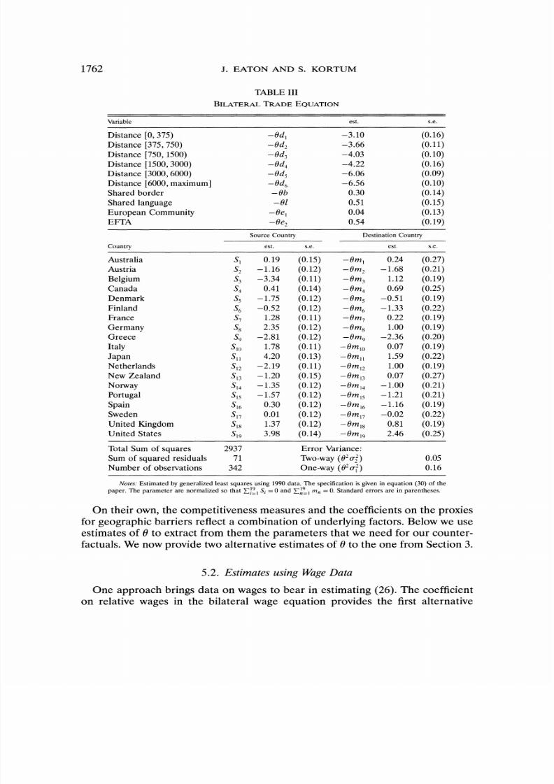
which we estimate by generalized least squares (GLS).35Table III reports the results. The estimates of the Si indicate that Japan is the
most competitive country in 1990, closely followed by the United States. Belgiumand Greece are the least competitive. As for geographic barriers, increaseddistance substantially inhibits trade, with its impact somewhat attenuated by ashared language, while borders, the EC, and EFTA do not play a major role. TheUnited States, Japan, and Belgium are the most open countries while Greece isleast open.36 Note that about a quarter of the total residual variance is reciprocal.
34An advantage of our formulation of distance effects is that it imposes little structure on how geo-
graphic barriers vary with distance. We explored the implications of the more standard specification
of geographic barriers as a quadratic function of distance. There were no differences worth reporting.35 To obtain the parameters of the variance-covariance matrix for GLS estimation we first estimate
the equationby OLS to obtaina set of residuals *i. We then estimateHO22by averagingnikin and62(r22+
- ) by averaging (k"i)236 Our finding about the openness of Japan may seem surprising given its low import share reported
in Table I. Analyses that ignore geography (for example, the first part of Harrigan (1996)), find
Japan closed. Once geography is taken into account, however, as (implicitly) later in Harrigan, it no
longer appears particularlyclosed. (Eaton and Tamura(1994) find Japan relatively more open to U.S.
exports than European countries as a group.) As equation (10) reveals, our concept of a country's
openness controls for both its location and its price level (as reflected by its price parameter P). Not
only is Japan remote, its competitiveness as a manufacturing supplier implies a high ', making it a
naturally tough market for foreigners to compete in. At the other extreme, our finding that Greece
is quite closed (even though it has a high import share) controls for both its proximity to foreignmanufacturing sources and its own inability to export much anywhere else.
7/28/2019 Ek Econometric a 2002
http://slidepdf.com/reader/full/ek-econometric-a-2002 23/40
1762 J. EATON AND S. KORTUM
TABLE III
BILATERAL TRADE EQUATION
Variable est. s.e.
Distance [0, 375) -0d1 -3.10 (0.16)
Distance [375, 750) -6d2 -3.66 (0.11)
Distance [750, 1500) -Od3 -4.03 (0.10)
Distance [1500,3000) -Od4 -4.22 (0.16)
Distance [3000, 6000) -Od5 -6.06 (0.09)
Distance [6000, maximum] - Od6 -6.56 (0.10)
Shared border -Ob 0.30 (0.14)
Shared language -01 0.51 (0.15)
European Community -0e1 0.04 (0.13)
EFTA -Oe2 0.54 (0.19)
Source Country Destination Country
Country est. s.e. est. s.e.
Australia S, 0.19 (0.15) -Om, 0.24 (0.27)
Austria S2 -1.16 (0.12) - m2 -1.68 (0.21)
Belgium S3 -3.34 (0.11) - m3 1.12 (0.19)
Canada S4 0.41 (0.14) - m4 0.69 (0.25)
Denmark S5 -1.75 (0.12) -6m5 -0.51 (0.19)
Finland S6 -0.52 (0.12) - m6 -1.33 (0.22)
France S7 1.28 (0.11) -6m7 0.22 (0.19)
Germany S8 2.35 (0.12) - m8 1.00 (0.19)
Greece S9 -2.81 (0.12) -6m9 -2.36 (0.20)
Italy S1( 1.78 (0.11) -6m10 0.07 (0.19)
Japan Sil 4.20 (0.13) -6m11 1.59 (0.22)Netherlands S12 -2.19 (0.11) -6m12 1.00 (0.19)
New Zealand S13 -1.20 (0.15) -Om13 0.07 (0.27)
Norway S14 -1.35 (0.12) -Om14 -1.00 (0.21)
Portugal S15 -1.57 (0.12) -6m15 -1.21 (0.21)
Spain S16 0.30 (0.12) -6m16 -1.16 (0.19)
Sweden S17 0.01 (0.12) -6m17 -0.02 (0.22)
United Kingdom S18 1.37 (0.12) -6m18 0.81 (0.19)
United States S19 3.98 (0.14) -6m19 2.46 (0.25)
Total Sum of squares 2937 Error Variance:
Sum of squared residuals 71 Two-way (02o2) 0.05
Number of observations 342 One-way (02o-2) 0.16
Notes: Estimated by generalized least squares using 1990 data. The specification is given in equation (30) of the
paper. The parameter are normalized so that E!9 Si = 0 and E19 mn = 0. Standard errors are in parentheses.
On their own, the competitiveness measures and the coefficients on the proxiesfor geographic barriersreflect a combination of underlying factors. Below we useestimates of 0 to extract from them the parameters that we need for our counter-factuals. We now provide two alternative estimates of 0 to the one from Section 3.
5.2. Estimates using WageData
One approach brings data on wages to bear in estimating (26). The coefficienton relative wages in the bilateral wage equation provides the first alternative
7/28/2019 Ek Econometric a 2002
http://slidepdf.com/reader/full/ek-econometric-a-2002 24/40
TECHNOLOGY, GEOGRAPHY, AND TRADE 1763
TABLE IV
DATA FOR ALTERNATIVE PARAMETERS
Research Years of Labor Force Density
Stock Schooling (HK adjusted) (pop/area)Country (U.S. = 1) (years/person) (U.S. = 1) (U.S. = 1)
Australia 0.0087 8.7 0.054 0.08Austria 0.0063 8.6 0.024 3.43Belgium 0.0151 9.4 0.029 12.02Canada 0.0299 10.0 0.094 0.10Denmark 0.0051 6.9 0.017 4.47Finland 0.0053 10.8 0.019 0.55France 0.1108 9.5 0.181 3.88Germany 0.1683 10.3 0.225 9.50Greece 0.0005 8.4 0.025 2.87
Italy 0.0445 9.1 0.159 7.16Japan 0.2492 9.5 0.544 12.42Netherlands 0.0278 9.5 0.043 13.64New Zealand 0.0010 9.3 0.010 0.47Norway 0.0057 9.2 0.015 0.49Portugal 0.0007 6.5 0.026 4.01Spain 0.0084 9.7 0.100 2.88Sweden 0.0206 9.6 0.031 0.71United Kingdom 0.1423 8.5 0.186 8.76United States 1.0000 12.1 1.000 1.00
Notes: Research stocks, in 1990, are from Coe and Helpman (1995). Average years of schooling Hi, in 1985,are from Kyriacou(1991). Labor forces, in 1990, are from Summers and Heston (1991). They are adjusted for
human capital by multiplyingthe country i figure by e 06H1.See the Appendix for complete definitions.
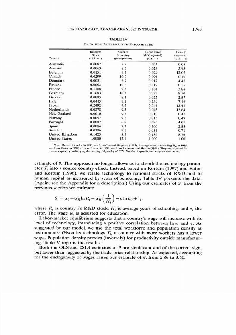
estimate of 0. This approach no longer allows us to absorb the technology param-eter Ti into a source country effect. Instead, based on Kortum (1997) and Eatonand Kortum (1996), we relate technology to national stocks of R&D and tohuman capital as measured by years of schooling. Table IV presents the data.(Again, see the Appendix for a description.) Using our estimates of Si from theprevious section we estimate
Si = aO+a lnRi-a (7Hj) -0 ln wi +ri-,
where Ri is country i's R&D stock, Hi is average years of schooling, and ri theerror. The wage wi is adjusted for education.
Labor-market equilibrium suggests that a country'swage will increase with itslevel of technology, introducing a positive correlation between lnw and r. Assuggested by our model, we use the total workforce and population density asinstruments: Given its technology Ti, a country with more workers has a lowerwage. Population density proxies (inversely) for productivityoutside manufactur-ing. Table V reports the results.
Both the OLS and 2SLS estimates of 0 are significant and of the correct sign,
but lower than suggested by the trade-price relationship. As expected, accountingfor the endogeneity of wages raises our estimate of 0, from 2.86 to 3.60.
7/28/2019 Ek Econometric a 2002
http://slidepdf.com/reader/full/ek-econometric-a-2002 25/40
1764 J. EATON AND S. KORTUM
TABLE V
COMPETITIVENESS EQUATION
Ordinary Two-Stage
Least Squares Least Squares
est. s.e. est. s.e.
Constant 3.75 (1.89) 3.82 (1.92)
Research stock, InRi aR 1.04 (0.17) 1.09 (0.18)
Human capital, l/Hi -aH -18.0 (20.6) -22.7 (21.3)
Wage, Inwi -0 -2.84 (1.02) -3.60 (1.21)
Total Sum of squares 80.3 80.3
Sum of squared residuals 18.5 19.1
Number of observations 19 19
Notes: Estimated using 1990 data. The dependent variable is the estimate Si of source-countrycompetitive-ness shown in Table III. Standard errors are in parentheses.
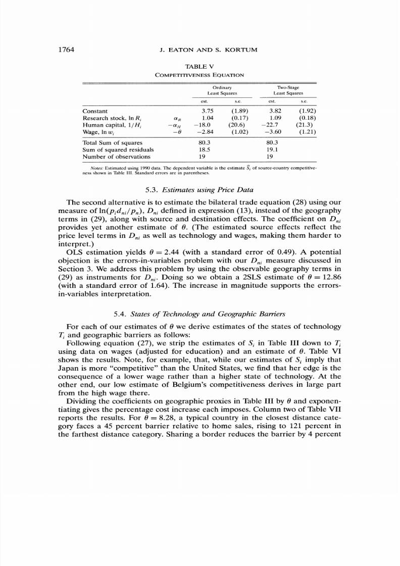
5.3. Estimates using Price Data
The second alternative is to estimate the bilateral trade equation (28) using our
measure of ln(pidi/Pn), Dni defined in expression (13), instead of the geographyterms in (29), along with source and destination effects. The coefficient on Dniprovides yet another estimate of 0. (The estimated source effects reflect the
price level terms in Dnias well as technology and wages, making them harder to
interpret.)OLS estimation yields 0 = 2.44 (with a standard error of 0.49). A potential
objection is the errors-in-variables problem with our Dni measure discussed in
Section 3. We address this problem by using the observable geography terms in
(29) as instruments for Dni. Doing so we obtain a 2SLS estimate of 0 = 12.86
(with a standard error of 1.64). The increase in magnitude supports the errors-
in-variables interpretation.
5.4. Statesof Technologyand GeographicBariers
For each of our estimates of 0 we derive estimates of the states of technology
Ti and geographic barriers as follows:
Following equation (27), we strip the estimates of Si in Table III down to Tiusing data on wages (adjusted for education) and an estimate of 0. Table VI
shows the results. Note, for example, that, while our estimates of Si imply that
Japan is more "competitive"than the United States, we find that her edge is the
consequence of a lower wage rather than a higher state of technology. At theother end, our low estimate of Belgium's competitiveness derives in large partfrom the high wage there.
Dividing the coefficients on geographic proxies in Table III by 0 and exponen-
tiating gives the percentage cost increase each imposes. Column two of Table VII
reports the results. For 0 = 8.28, a typical country in the closest distance cate-
gory faces a 45 percent barrier relative to home sales, rising to 121 percent inthe farthest distance category. Sharing a border reduces the barrierby 4 percent

7/28/2019 Ek Econometric a 2002
http://slidepdf.com/reader/full/ek-econometric-a-2002 26/40
TECHNOLOGY, GEOGRAPHY, AND TRADE 1765
TABLE VI
STATES OF TECHNOLOGY
Estimated Implied
Source-countryStates of Technology
Country Competitiveness 0 = 8.28 0 = 3.60 0 = 12.86
Australia 0.19 0.27 0.36 0.20
Austria -1.16 0.26 0.30 0.23
Belgium -3.34 0.24 0.22 0.26
Canada 0.41 0.46 0.47 0.46
Denmark -1.75 0.35 0.32 0.38
Finland -0.52 0.45 0.41 0.50
France 1.28 0.64 0.60 0.69
Germany 2.35 0.81 0.75 0.86
Greece -2.81 0.07 0.14 0.04
Italy 1.78 0.50 0.57 0.45
Japan 4.20 0.89 0.97 0.81
Netherlands -2.19 0.30 0.28 0.32
New Zealand -1.20 0.12 0.22 0.07
Norway -1.35 0.43 0.37 0.50
Portugal -1.57 0.04 0.13 0.01
Spain 0.30 0.21 0.33 0.14
Sweden 0.01 0.51 0.47 0.57
United Kingdom 1.37 0.49 0.53 0.44
United States 3.98 1.00 1.00 1.00
Notes: The estimates of source-country competitiveness are the same as those shown in Table III. For an
estimatedparameter
Si, theimplied
state oftechnology
isTi
=(eSi w9)f6. States
oftechnology
arenormalizedrelative to the U.S. value.
while sharing a language reduces it by 6 percent. It costs 25 percent less to exportinto the United States, the most open country, than to the average country. At
the high end it costs 33 percent more to export to Greece than to the averagecountry.37 Moving to the alternative values of 0 affects the implied geographicbarriers in the opposite direction. Even for our high value of 0, however, geo-graphic barriers appear substantial.
Our simple method-of-moments estimator of 0 = 8.28 from Section 3 lies verymuch in the middle of the range of estimates we obtain from our alternative
approaches, 0 = 3.60 using wage data and 0 = 12.86 using price data. Hence,except where noted, we use it (and the consequent value of Ti and d"j) in theanalysis that follows.38
37 Wei (1996) obtains very similar results from a gravity model making the Armington assumption
that each country produces a unique set of commodities. He does not estimate the elasticity of
substitution between goods from different countries, but picks a value of 10 as his base. As discussed,
the Armington elasticity plays a role like our parameter 0. Hummels (2002) relates data on actual
freight costs for goods imported by the United States and a small number of other countries to
geographical variables. His finding of a 0.3 elasticity of cost with respect to distance is reflected,
roughly, in our estimates here.38 Our estimates of 0, obtained from different data using different methodologies, differ substan-
tially. Nonetheless, they are in the range of Armington elasticities for imports used in computablegeneral equilibrium models. See, for example, Hertel (1997).

7/28/2019 Ek Econometric a 2002
http://slidepdf.com/reader/full/ek-econometric-a-2002 27/40
1766 J. EATON AND S. KORTUM
TABLE VII
GEOGRAPHIC BARRIERS
Estimated Implied
Geography Barrier's% Effect on Cost
Source of Barrier Parameters 0= 8.28 0 =3.60 0 =12.86
Distance [0, 375) -3.10 45.39 136.51 27.25
Distance [375, 750) -3.66 55.67 176.74 32.97
Distance [750, 1500) -4.03 62.77 206.65 36.85
Distance [1500,3000) -4.22 66.44 222.75 38.82
Distance [3000, 6000) -6.06 108.02 439.04 60.25
Distance [6000, maximum] -6.56 120.82 518.43 66.54
Shared border 0.30 -3.51 -7.89 -2.27
Shared language 0.51 -5.99 -13.25 -3.90
European Community 0.04 -0.44 -1.02 -0.29
EFTA 0.54 -6.28 -13.85 -4.09
Destination country:Australia 0.24 -2.81 -6.35 -1.82
Austria -1.68 22.46 59.37 13.94
Belgium 1.12 -12.65 -26.74 -8.34
Canada 0.69 -7.99 -17.42 -5.22
Denmark -0.51 6.33 15.15 4.03
Finland -1.33 17.49 44.88 10.94
France 0.22 -2.61 -5.90 -1.69
Germany 1.00 -11.39 -24.27 -7.49
Greece -2.36 32.93 92.45 20.11
Italy 0.07 -0.86 -1.97 -0.56Japan 1.59 -17.43 -35.62 -11.60
Netherlands 1.00 -11.42 -24.33 -7.51
New Zealand 0.07 -0.80 -1.83 -0.52
Norway -1.00 12.85 32.06 8.10
Portugal -1.21 15.69 39.82 9.84
Spain -1.16 14.98 37.85 9.40
Sweden -0.02 0.30 0.69 0.19
United Kingdom 0.81 -9.36 -20.23 -6.13
United States 2.46 -25.70 -49.49 -17.40
Notes: The estimated parameters governing geographic barriers are the same as those shown in Table III.
For an estimated parameter d, the implied percentage effect on cost is 100(e-d/ - 1).
6. COUNTERFACTUALS
The estimation presented in Section 5 provides parameter values that allow us
to quantify the full model, enabling us to pursue an analysis of counterfactuals.
Given that the model is highly stylized (we have, for example, suppressed hetero-
geneity in geographic barriers across manufacturing goods), these counterfactuals
should not be seen as definitive policy analysis. But regardless of how indicative
they are of actual magnitudes, they do provide insight into the workings of themodel.

7/28/2019 Ek Econometric a 2002
http://slidepdf.com/reader/full/ek-econometric-a-2002 28/40
TECHNOLOGY, GEOGRAPHY, AND TRADE 1767
TABLE VIII
SUMMARY OF PARAMETERS
Parameter Definition Value Source
0 comparative advantage 8.28 (3.60, 12.86) Section 3 (Section 5.2, Section 5.3)
a manufacturing share 0.13 production and trade data
,B labor share in costs 0.21 wage costs in gross output
Ti states of technology Table VI source effects stripped of wages
dni geographic barriers Table VII geographic proxies adjusted for 0
To complete the parameterization we calculate a = 0.13, the average demandfor final manufactures as a fraction of GDP.39 Table VIII summarizes the
structural parameters of the model, their definitions, the values we assign tothem, and where we got these numbers.
We can examine counterfactuals according to a number of different criteria.One is overall welfare in country n, measured as real GDP: Wn = Yn/pa. (Sincenonmanufactures are numeraire, the price level in country n is pa. Since wehold labor supplies and populations fixed throughout, there is no need to distin-guish between GDP and GDP per worker or GDP per capita.) Decomposing thechange in welfare into income and price effects gives
In - -In- aIn- ' __ a In-
Wn Yn Pn wn Yn Pn
(Here x' denotes the counterfactual value of a variablexn.) In the case of mobilelabor, of course, only the price effect is operative. Aside from looking at welfare,for the case of mobile labor, we ask about manufacturing employment while,for the case of immobile labor, we look at the manufacturingwage wn. We alsoinvestigate how trade patterns change.
Since we have data on both manufacturing employment and manufacturingwages, we can look at our model's implications for each given data on the other.Our fit is not perfect since we (i) impose a common manufacturing demandshare a across countries and
(ii) ignoresources of manufactures from
outsideour sample of 19 OECD countries.We wish to distinguish the effects of any of the counterfactuals we examine
in the next section from the initial misfit of our model. We therefore comparethe various counterfactuals that we examine with a baseline in which wages are
39Specifically we solve for a from the relationship
X. +IMP,n=
(1-/3)(Xnn +EXP) +aYn
summed across our sample (with ,B= .21) in 1990. Here IMPn is manufacturing imports and EXPnis manufacturing exports, and Yn is total GDP, each translated from local currency values into U.S.dollars at the official exchange rate.
7/28/2019 Ek Econometric a 2002
http://slidepdf.com/reader/full/ek-econometric-a-2002 29/40
1768 J. EATON AND S. KORTUM
calculated to be consistent with equations (16), (17), and (20), given actual man-ufacturing employment and GDP. Comparing these baseline wages with actual
data the root mean square error is 5.0 percent.40In performing counterfactuals we proceed as follows: With mobile labor we
treat total GDP and wages as fixed. We set GDPs to their actual levels andwages to the baseline. With immobile labor we treat nonmanufacturingGDP andmanufacturing employment as fixed. We set manufacturing employment to itsactual level and nonmanufacturing GDP to actual GDP less the baseline valuefor labor income in manufacturing(actual employment times the baseline wage).
6.1. The Gains from Trade
We first consider the effects of raising geographic barriers to their autarkylevels (dni -? cc for n =A). We then perform what turns out to be the moreextreme exercise of asking what would happen in a zero-gravity world with nogeographic barriers (with all dni = 41
Table IX shows what happens in a move to autarkyfor each of our 19 coun-tries. The first column reports the welfare loss in the case of mobile labor. Thecosts of moving to autarky range from one quarter of a percent for Japan up toten percent for Belgium.42While these costs appear modest, it should be remem-bered that they reflect the effects of shutting down trade only in manufacturesand hence understate the loss from not trading at all.43Manufacturing labor,
shown in column three, rises everywhere except in Germany, Japan, Sweden,and the United Kingdom. That manufacturingemployment shrinks in these four
40 Our model overstates the Canadian wage by 21 percent, but otherwise predictions are quiteclose. With our estimated parameters, equation (30) predicts much more trade between Canadaand the United States than actually occurs. Since U.S. purchases loom large in Canada, its labor
market equilibrium condition (18) implies more demand for Canadian manufacturing labor than
there really is.41For simplicity,we ignore any tariff revenues that geographic barriersmight generate. We consider
the effect of reducing tariff barriers, taking revenue effects into account, in Section 6.4 below.42 In the mobile labor case (with total GDP and the manufacturing wage fixed) the only welfare
effect is from the decline in the manufacturing price level, which affects welfare with an elasticitya. As a consequence we can use expression (15) to obtain a simple analytic formula for the welfare
effect of moving to autarky:
WI a
InIn
3
It follows that the gains from trade vary inversely with 0. The implied gains from trade more than
double, for example, using our lower estimate of 0 = 3.60.43Since most trade is in manufactures, we could try to argue that we have captured most of the
gains from trade. But trade volume may be a poor indicator of the gains from trade in other sectorsrelative to manufacturing. Since productivity in agriculture or mining is likely to be much more
heterogeneous across countries, applying our model to trade in these goods could well deliver a much
lower value of 0. An implication is that eliminating what trade does occur would inflict much moredamage.

7/28/2019 Ek Econometric a 2002
http://slidepdf.com/reader/full/ek-econometric-a-2002 30/40
TECHNOLOGY, GEOGRAPHY, AND TRADE 1769
TABLE IX
THE GAINS FROM TRADE: RAISING GEOGRAPHIC BARRIERS
Percentage Change from Baseline to Autarky
Mobile Labor Immobile Labor
Country Welfare Mfg. Prices Mfg. Labor Welfare Mfg. Prices Mfg. Wages
Australia -1.5 11.1 48.7 -3.0 65.6 54.5
Austria -3.2 24.1 3.9 -3.3 28.6 4.5
Belgium -10.3 76.0 2.8 -10.3 79.2 3.2
Canada -6.5 48.4 6.6 -6.6 55.9 7.6
Denmark -5.5 40.5 16.3 -5.6 59.1 18.6
Finland -2.4 18.1 8.5 -2.5 27.9 9.7
France -2.5 18.2 8.6 -2.5 28.0 9.8
Germany -1.7 12.8 -38.7 -3.1 -33.6 -46.3
Greece -3.2 24.1 84.9 -7.3 117.5 93.4Italy -1.7 12.7 7.3 -1.7 21.1 8.4
Japan -0.2 1.6 -8.6 -0.3 -8.4 -10.0
Netherlands -8.7 64.2 18.4 -8.9 85.2 21.0
New Zealand -2.9 21.2 36.8 -3.8 62.7 41.4
Norway -4.3 32.1 41.1 -5.4 78.3 46.2
Portugal -3.4 25.3 25.1 -3.9 53.8 28.4
Spain -1.4 10.4 19.8 -1.7 32.9 22.5
Sweden -3.2 23.6 -3.7 -3.2 19.3 -4.3
United Kingdom -2.6 19.2 -6.0 -2.6 12.3 -6.9
United States -0.8 6.3 8.1 -0.9 15.5 9.3
Notes: All percentage changes are calculated as 100ln(x'/x) where x' is the outcome under autarky (d,j oo or n :A ) and
x is the outcome in the baseline.
when trade is shut down could be seen as indicating their overall comparative
advantage in manufactures.The remaining columns consider the effects of moving to autarky with immo-
bile labor. Column four reports the welfare loss. The effect on welfare is more
negative than when labor is mobile, but usually only slightlyso.
The net welfare effects mask larger changes in prices and incomes. In all
but the four "natural manufacturers" (Germany, Japan, Sweden, the United
Kingdom), the price rise is greater when manufacturing labor is immobile. (In
Germany and Japan manufacturing prices actually fall.) But these greater pricechanges lead to only slightly larger effects on welfare because they are mitigatedby wage changes (reported in column six): The wage in manufacturing rises in
all but the four "naturalmanufacturers."44
44 How much labor force immobility exacerbates the damage inflicted by autarky depends on the
extent of specialization in manufacturing.A move to autarkyraises the manufacturing wage the most
in Greece, with the smallest manufacturing share. But since its share of manufacturing labor income
(reported in Table I) is so small, the overall welfare effect is swamped by the large increase in
manufacturing prices. In Germany, with the largest manufacturing share, a move to autarky lowers
the manufacturing wage. But since the share of manufacturing is so large, the welfare cost of this loss
in income is not offset by the drop in manufacturing prices. For countries that are less specialized(in or away from manufactures), labor mobility makes less difference for overall welfare.
7/28/2019 Ek Econometric a 2002
http://slidepdf.com/reader/full/ek-econometric-a-2002 31/40
7/28/2019 Ek Econometric a 2002
http://slidepdf.com/reader/full/ek-econometric-a-2002 32/40
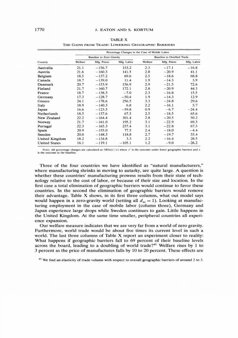
TECHNOLOGY, GEOGRAPHY, AND TRADE 1771
of the same order of magnitude as the costs of moving to autarky, but withlessvariation around the mean. We already see the United States and Japan losing
their size-based edge in manufactures from this more modest drop in geographicbarriers, while manufacturingin most small countries rises.
6.2. Technologyvs. Geography
Our discussion of the gains from trade has already brought up the question,raised in the economic geography literature, of the roles of geography andtech-nology in determining specialization. To allow specialization to vary, we considerthe case in which labor is mobile. With zero gravity the fraction of a country'slabor force devoted to manufacturing is then proportional to (T1/Lj)/w1+0', sodepends only on the state of technology per worker and the wage. When geo-graphic barriers are prohibitive the fraction is simply a, the share of manufac-tures in final demand, so that not even technology matters. But in neither caseis geography relevant.
How do technology and geography compete in determining comparative
advantage in between these extremes? Looking at what happens to the fractionof labor devoted to manufacturing as geographic barriers fall, two basic pat-terns emerge. For smaller countries manufacturing shrinks as geographic barri-ers diminish from their autarkylevel. Production shifts to larger countries whereinputs are cheaper. As geographic barriers continue to fall, however, the forces oftechnology take over, and the fraction of the labor force in manufacturinggrows,
often exceeding its autarkylevel. The results for Denmark, depicted in Figure 3,illustrate this pattern nicely. For the largest countries in our sample, Germany,Japan, and the United States, the pattern is reversed. Their manufacturing sec-tor at first grows and then shrinks as geographic barriers fall. Germany, alsodepicted in Figure 3, illustrates the pattern most starkly.
Extant geographic barriers place the world near a transition between onewhere the effects of geography dominate and one where technology governs com-
parative advantage. The results suggest a decline in barriers would lead to spe-cialization more along Ricardian lines, with large countries starting to lose theiredge.46
6.3. The Benefits of Foreign Technology
With geographic barriers as high as they are, how much does trade spreadthe benefit of a local improvement in technology? We increase the state of
46Whether a further decline in geographic barriers (defined in the iceberg sense here) is in the
works is an open question. Recent increases in trade volumes relative to output may have created
a perception that technical progress in communication and transport is feeding an inexorable trend
toward lower geographic barriers. Our model illustrates how, in order to increase trade, the rate of
progress in international transactions must exceed that in production. A proportional increase in all
states of technology Ti has no effect on trade shares. The reason is that technical progress implies a
proportional reduction in the cost of delivering goods to any destination, whether at home or abroad,so does not affect the margin at which goods are imported or produced locally.
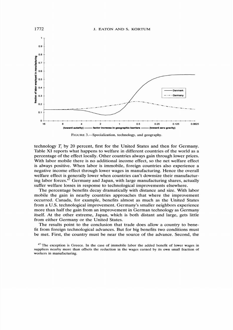
7/28/2019 Ek Econometric a 2002
http://slidepdf.com/reader/full/ek-econometric-a-2002 33/40
1772 J. EATON AND S. KORTUM
0.9
0.8
c |! 0.7-
E 0.6
o 0.5
o 0.40.4- / J~~~~~~~~~~~~~~~~~~Denma
0
r 0.3 Germany-0
0.2
0.1
0 l l l l l l l l l l l l l l l l l l l l l l I
16 8 4 2 1 0.5 0.25 0.125 0.0625
(towardautarky) factor increase Ingeographic barriers (toward zero gravity)
FIGURE 3.-Specialization, technology, and geography.
technology T1by 20 percent, first for the United States and then for Germany.Table XI reports what happens to welfare in different countries of the world as apercentage of the effect locally. Other countries alwaysgain through lower prices.With labor mobile there is no additional income effect, so the net welfare effectis always positive. When labor is immobile, foreign countries also experience anegative income effect through lower wages in manufacturing.Hence the overallwelfare effect is generally lower when countries can't downsize their manufactur-ing labor forces.47Germany and Japan, with large manufacturingshares, actuallysuffer welfare losses in response to technological improvements elsewhere.
The percentage benefits decay dramaticallywith distance and size. With labormobile the gain in nearby countries approaches that where the improvement
occurred. Canada, for example, benefits almost as much as the United Statesfrom a U.S. technological improvement. Germany's smaller neighbors experiencemore than half the gain from an improvement in German technology as Germanyitself. At the other extreme, Japan, which is both distant and large, gets littlefrom either Germany or the United States.
The results point to the conclusion that trade does allow a country to bene-fit from foreign technological advances. But for big benefits two conditions mustbe met. First, the country must be near the source of the advance. Second, the
47The exception is Greece. In the case of immobile labor the added benefit of lower wages in
suppliers nearby more than offsets the reduction in the wages earned by its own small fraction ofworkers in manufacturing.

7/28/2019 Ek Econometric a 2002
http://slidepdf.com/reader/full/ek-econometric-a-2002 34/40

7/28/2019 Ek Econometric a 2002
http://slidepdf.com/reader/full/ek-econometric-a-2002 35/40
1774 J. EATON AND S. KORTUM
tariffs, (ii) the United States removes its tariff unilaterally, and (iii) members ofthe European Community (as of 1990) drop tariffs against each other.
GeneralMultilateralTariffElimination:
Welfare rises almost everywhere if all 19 countries collectively remove tariffs.The benefits are substantially greater with mobile labor, varying from a high of1.31 percent for Belgium to a low of 0.21 percent for Japan, with most countriesgaining around one percent. With immobile labor the gains never exceed half apercent. Germany actually experiences a 0.05 percent loss (losing more in tariffrevenue than its gain from lower prices and a slightly higher wage in manufac-turing).
U.S. UnilateralTariffElimination:
If the United States removes tariffs on its own, everyone benefits except theUnited States, which, for standardoptimal tariff reasons, suffers a welfare loss of0.005 percent with mobile labor (0.13 percent with immobile labor). The biggestwinner is Canada, which enjoys a welfare gain of 0.5 percent with mobile labor(1.1 percent with immobile labor).
With mobile labor, the percentage gains for other countries roughly equal orexceed the U.S. loss. The results point to the importance of pursuing freer trademultilaterally,since the benefits to the rest of the world of U.S. liberalization farexceed the cost to the United States.
TradeDiversion in the European Community:
Table XII reports some effects of eliminating tariffs within the 1990 EuropeanCommunity. Who gains and who loses depends very much on the mobility oflabor. As the second column reports, with immobile labor the major losers arenonmembers nearby, whose manufacturing wages must fall in order for themto remain competitive suppliers to the EC. Members of the EC consequentlybenefit from lower external prices and a greater premium placed on their ownmanufacturingworkers.
With mobile labor, however, the losers (as reported in the first column) arethe northern EC members. In this scenario workers in nonmember states moveto other activities rather than suffer wage cuts. Northern EC members divertimports from these nonmember states to less efficient southern EC sources.
Note from the third and fourth columns that with market integration, intra-EC trade expands substantially, especially when labor is mobile. Moreover, inthe mobile labor case, EC market share elsewhere generally expands: By mak-ing inputs cheaper, market integration provides EC countries a cost advantageoutside.
7. CONCLUSION
Comparative advantagecreates potential gains from trade. The extent to whichthese gains are realized, however, is attenuated by the resistance imposed by

7/28/2019 Ek Econometric a 2002
http://slidepdf.com/reader/full/ek-econometric-a-2002 36/40
TECHNOLOGY, GEOGRAPHY, AND TRADE 1775
TABLE XII
THE EUROPEAN COMMUNITY: WELFARE AND TRADE
Effect of Removing all Tariffs on Intra-EC Trade
Aggregate Welfare Imports from the EC
Country Mobile Labor Immobile Labor Mobile Labor Immobile Labor
Australia 0.13 0.11 27.7 2.8
Austria 0.32 -0.07 -1.9 -3.4
Belgium* -0.91 0.54 61.3 26.3
Canada 0.01 0.01 28.0 2.2
Denmark* -0.27 0.18 49.9 30.8
Finland 0.28 -0.02 4.6 -2.9
France* 0.08 0.05 46.3 33.7
Germany* -0.03 -0.03 58.5 41.9
Greece* 0.28 0.13 30.8 24.0Italy* 0.14 0.04 44.9 36.4
Japan 0.07 -0.01 32.4 2.3
Netherlands* -0.58 0.33 56.3 26.9
New Zealand 0.14 0.09 24.1 1.9
Norway 0.34 0.05 3.2 -2.9
Portugal* 0.03 0.10 44.0 32.8
Spain* 0.21 0.05 43.7 34.3
Sweden 0.31 -0.10 2.0 -3.3
United Kingdom* -0.02 0.02 51.9 36.1
United States 0.10 0.03 27.8 2.2
Notes: All numbers are percentage changes from the baseline. In the baseline all trade is subject to a 5
percent tariff. The counterfactual is to remove tariffs between members (as of 1990) of the EC (appearing witha *). Each pair of columns shows the results of performing the counterfactual first for the case of mobile laborand then for the case of immobile labor.
geographic barriers. We have developed a Ricardian model that captures these
two forces quite parsimoniously. The model delivers equations relating bilateral
trade around the world to parameters of technology and geography. We use dataon bilateral trade flows, prices, and geography to estimate the parameters.
While the gravity literature has recognized the importance of geographic bar-
riers in curtailing trade flows, formal models of international trade have typically
ignored them. The exceptions are models in which specialization is preordained
by product differentiation,via either the
Armington assumptionor
monopolis-tic competition. In contrast, our framework allows geographic barriers as well as
technology to determine specialization. It also connects trade flows to the devi-
ations from the law of one price that geographic barriers generate.
Dept. of Economics, New YorkUniversity,269 MercerSt., New York,NY 10003,U S.A., and NBER; jonathan.eaton@nyu. edu; http://econ.nyu.edu/user/eatonj
and
Dept. of Economics, University of Minnesota, 1035 Heller Hall, Minneapolis,MN 55455, U.S.A., and NBER; [email protected];http://www.econ.umn.edu/-kortum/
ManuscriptreceivedJuly, 2000; final revision receivedMay, 2001.

7/28/2019 Ek Econometric a 2002
http://slidepdf.com/reader/full/ek-econometric-a-2002 37/40
1776 J. EATON AND S. KORTUM
APPENDIX
Our analysis uses data for manufacturing in 1990 for the 19 OECD countries listed in Table I.
TradeData:
Our dependent variables are transformations (discussed in the text) of bilateral manufacturing
imports. Country i's imports from home are gross manufacturing production less manufacturing
exports. Its total manufacturing expenditures are home purchases plus imports from everywhere else.
These measures are reported by the STAN database in local currencies (OECD (1995)). We calculate
imports from each of the other 18 countries, as a fraction of total manufactured imports, based on
the United Nations-Statistics Canada bilateral merchandise trade data by 4-digit SITC, as described
in Feenstra, Lipsey, and Bowen (1997).49 All import measures are c.i.f. Since our dependent variables
normalize imports either by home sales or by total expenditures, no exchange rate translation is
required.
The first column of Table I shows that imports typically represent less than half of spending onmanufactures, the exceptions being Belgium, the Netherlands, and Denmark. The second column
shows that most of the imports of our sample of 19 OECD countries are purchased from one of the
other 18 countries in the sample.
Price Data:
Prices in 1990 for over 100 GDP categories in each of our 19 countries are from World Bank
(1993). We use the 50 items identified by Hooper and Vrankovich (1995) as corresponding to either:
(i) textile, apparel, and leather products, (ii) machinery, equipment, and fabricated metal products,
or (iii) other manufactured products. We dropped the many items related to food and chemicals
since we thought their prices would be unduly influenced by proximity to natural resources and taxes
on petroleum products, two factors absent from our model.
Proxies or GeographicBariers:
Distances between countries serve as a determinant of geographic barriers. The distances are
in thousands of miles measured between central cities in each country. (A list of the cities is in
Eaton and Tamura (1994).) Language groups are: (i) English (Australia, Canada, New Zealand,
United Kingdom, United States), (ii) French (Belgium and France), and (iii) German (Austria and
Germany).
ManufacturingEmploymentand Wages:
Since we use the model itself to solve for the price of intermediates, the only input costs entering
our empirical trade equations are manufacturing wages. Annual compensation per worker in manu-
facturing (which includes employers' compulsory pension and medical payments) is reported by the
OECD (1995) in local currency.We translate into U.S. dollars at the current exchange rates to obtain
measured compensation compi, reported in the third column of Table 1.50We then adjust by worker
quality, setting wi = (compi)e Hi, where Hi is average years of schooling and g is the return to
education. Column four of Table I reports the human-capital adjusted wage (human-capital adjusted
manufacturing employment is shown in column five). We set g = .06, which Bils and Klenow (2000)
suggest is a conservative estimate. Years of schooling is from Kyriacou (1991), as shown in Table IV
49We used the concordance of Maskus (1991) to determine those SITC codes corresponding to
manufactures. Using the concordance in Feenstra, Lipsey, and Bowen (1997) made virtually no dif-
ference.
50 We use the official rather than the purchasing power exchange rate since it determines differ-ences in costs of production. In our model, differences in purchasing power arise endogenously.

7/28/2019 Ek Econometric a 2002
http://slidepdf.com/reader/full/ek-econometric-a-2002 38/40
TECHNOLOGY, GEOGRAPHY, AND TRADE 1777
AggregateIncome:
In our counterfactuals we require total income in 1990. We use local-currency GDP in 1990 (from
OECD (1997)) translated into U.S. dollars at the 1990 exchange rate. The last column of Table Ishows manufacturing labor income as a percentage of total income.
Data for Alternative Parameters:
Table IV shows the data used to pursue our alternative estimate of 0, as described in Section 5.2.
The first column shows stocks of research Ri for each country, from Coe and Helpman (1995). They
use the perpetual inventory method (assuming a depreciation rate of five percent) to add up real
R&D investment by business enterprises. The second column shows the human capital measure Hi,for which we use average years of schooling in 1985 from Kyriacou (1991).
We use two variables to instrument for wage costs. The first is aggregate workforce worki, from
Summers and Heston (1991, version 5.6), shown in the third column of Table IV. As with wages,
we adjust for education setting Li = (worki)egHi.The second instrument is density, defined as the
aggregate workforce divided by a country's land area, shown in the last column of Table IV.
REFERENCES
ANDERSON,J. E. (1979): "A Theoretical Foundation for the Gravity Equation," American Economic
Review, 69, 106-116.
ANDERSON,J. E., AND E. VANWINCOOP2001): "Gravitywith Gravitas: A Solution to the Border
Puzzle," NBER Working Paper No. 8079.
ANDERSON,S. P., A. DE PALMA,AND J. THISSE 1992): Discrete Choice Theoryof Product Differen-
tiation. Cambridge, MA: MIT Press.
ARMINGTON, P. S. (1969): "A Theory of Demand for Products Distinguished by Place of Produc-
tion," IMF Staff Papers No. 16.BAXTER,M. (1992): "Fiscal Policy, Specialization, and Trade in the Two-Sector Model: The Return
of Ricardo?" Journal of Political Economy, 100, 713-744.
BERNARD,A. B., J. EATON,J. B. JENSEN, AND S. KORTUM (2000): "Plants and Productivity in
International Trade," NBER Working Paper No. 7688.
BERNARD,A. B., AND J. B. JENSEN (1999): "Exceptional Exporter Performance: Cause, Effect, or
Both?" Journal of InternationalEconomics, 47, 1-25.
BERGSTRAND, J. (1989): "The Generalized Gravity Equation, Monopolistic Competition, and Factor
Proportions Theory in International Trade," Review of Economics and Statistics,71, 143-153.
BERRY, S. T. (1994): "Estimating Discrete-Choice Models of Product Differentiation," Rand Journal
of Economics, 71, 242-262.
BILLINGSLEY, P. (1986): Probabilityand Measure, 2nd edition. New York: John Wiley and Sons.
BILS, M., AND P. J. KLENOW (2000): "Does Schooling Cause Growth?"American Economic Review,
90, 1160-1183.
CHOUDHRI, E. U., AND L. L. SCHEMBRI (forthcoming): "Productivity Performance and Interna-
tional Competitiveness: A New Test of an Old Theory," forthcoming in Canadian Journal of Eco-
nomics.
COE,D. T., AND E. HELPMAN (1995): "International R&D Spillovers," EuropeanEconomic Review,
39, 859-887.
CRUCINI, M. J., C. I. TELMER, AND M. ZACHARIADIS (2001): "Understanding European Real
Exchange Rates," Vanderbilt Working Paper 01-W20.
DAVIS,D. R. (1998): "The Home Market, Trade, and Industrial Structure,"American Economic
Review, 88, 1264-1276.
DAVIS,D. R., AND D. E. WEINSTEIN (2001): "An Account of Global Factor Trade," American
Economic Review, 91, 1423-1453.
DEARDORFF, A. V. (1984): "Testing Trade Theories and Predicting Trade Flows," in Handbook ofInternationalEconomics, VolumeI, ed. by R. Jones and P. Kenen. Amsterdam: North-Holland.

7/28/2019 Ek Econometric a 2002
http://slidepdf.com/reader/full/ek-econometric-a-2002 39/40
1778 J. EATON AND S. KORTUM
DORNBUSCH, R., S. FISCHER, AND P. A. SAMUELSON (1977): "Comparative Advantage, Trade,and Payments in a Ricardian Model with a Continuum of Goods," American Economic Review, 67,823-839.
EATON, J., AND S. KORTUM (1996): "Trade in Ideas: Patenting and Productivity in the OECD,"Journal of InternationalEconomics, 40, 251-278.
(1999): "International Technology Diffusion: Theory and Measurement," International Eco-
nomic Review, 40, 537-570.
EATON, J., AND A. TAMURA (1994): "Bilateralism and Regionalism in Japanese and U.S. Trade
and Direct Foreign Investment Patterns," Journal of the Japanese and InternationalEconomies, 8,478-510.
ENGEL, C., AND J. H. ROGERS (1996): "How Wide is the Border?" American Economic Review, 86,1112-1125.
EVENETT, S. J., AND W. KELLER (2002): "On Theories Explaining the Success of the Gravity Equa-
tion," Journal of Political Economy, 110, 281-316.
FEENSTRA, R. C., R. E. LIPSEY, AND H. P. BOWEN (1997): "World Trade Flows, 1970-1992, with
Production and TariffData," NBER Working Paper No. 5910.FRIEDMAN, M. (1957): A Theoryof the Consumption Function. Princeton, NJ: Princeton University
Press.
GROSSMAN, G. M., AND E. HELPMAN (1995): "Technologyand Trade,"in The Handbook of Interna-tional Economics, VolumeIII, ed. by G. M. Grossman and K. Rogoff. Amsterdam: North-Holland.
HARRIGAN, J. (1996): "Openness to Trade in Manufactures in the OECD," Journal of InternationalEconomics, 40, 23-39.
(1997): "Technology, Factor Supplies, and International Specialization: Estimating the Neo-
classical Model," American Economic Review, 87, 475-494.
HAVEMAN, J., AND D. HUMMELS (2002): "Alternative Hypotheses and the Volume of Trade: The
Gravity Equation and the Extent of Specialization," Purdue University Working Paper.HELPMAN, E. (1987): "Imperfect Competition and International Trade: Evidence from Fourteen
Industrial Countries," Journal of Japanese and InternationalEconomics, 1, 62-81.HERTEL, T. W. (1997): Global TradeAnalysis: Modeling and Applications. Cambridge: Cambridge
University Press.
HOOPER, P., AND E. VRANKOVICH (1995): "International Comparisons of the Levels of Unit LaborCosts in Manufacturing,"International Finance Discussion Papers No. 527.
HUMMELS, D. (2002): "Toward a Geography of Trade Costs," Purdue University Working Paper.HUMMELS, D., AND J. LEVINSOHN (1995):"Monopolistic Competition and International Trade:
Reconsidering the Evidence," Quarterly ournal of Economics, 110, 799-836.
HUMMELS, D., D. RAPOPORT, AND K. YI (1998): "VerticalSpecialization and the Changing Natureof World Trade,"FRBNY Economic Policy Review, 4, 79-99.
JENSEN, P. E. (2000): "Analysis of Bilateral Trade Patterns with Panel Data," Reviewof InternationalEconomics, 8, 86-99.
JOHNSON, N. L., AND S. KOTZ (1970): Continuous UnivariateDistributions. Boston: Houghton and
Mifflin.KORTUM, S. (1997): "Research, Patenting, and Technological Change," Econometrica, 65, 1389-1419.KRUGMAN, P. R. (1991): Geographyand Trade.Cambridge, MA: MIT Press.
(1995): "IncreasingReturns, Imperfect Competition, and the Positive Theory of InternationalTrade," in The Handbook of International Economics, Volume III, ed. by G. M. Grossman andK. Rogoff. Amsterdam: North-Holland.
KRUGMAN, P. R., AND A. J. VENABLES (1995): "Globalization and the Inequality of Nations,"Quarterly ournal of Economics, 110, 857-880.
KYRIACOU, G. (1991): "Level and Growth Effects of Human Capital," C. V Starr Center Working
Paper 91-26.
LEAMER, E. (1984): Sources of International Comparative Advantage: Theory and Evidence.Cambridge, MA: MIT Press.
LEAMER, E., AND J. LEVINSOHN (1995): "International Trade Theory: The Evidence," in The Hand-
book of InternationalEconomics, VolumeIII, ed. by G. M. Grossman and K. Rogoff. Amsterdam:North-Holland.

7/28/2019 Ek Econometric a 2002
http://slidepdf.com/reader/full/ek-econometric-a-2002 40/40
TECHNOLOGY, GEOGRAPHY, AND TRADE 1779
MAcDOUGALL,G. D. A. (1951): "British and American Exports: A Study Suggested by the Theory
of Comparative Costs (Part I)," Economic Journal, 61, 697-724.
(1952): "British and American Exports: A Study Suggested by the Theory of Comparative
Costs (Part II)," Economic Journal, 62, 487-521.
MASKUS, K. (1991): "ComparingInternational Trade Data and Product and National Characteristics
Data for the Analysis of Trade Models," in International Economic Transactions: ssues in Measure-
ment and EmpiricalResearch,National Bureau of Economic Research Studies in Income and Wealth,
Volume 55, ed. by P. Hooper and J. D. Richardson. Chicago: University of Chicago Press.
McFADDEN, D. P. (1974): "Conditional Logit Analysis of Qualitative Choice Behavior," in Frontiersin Econometrics, ed. by P. Zarembka. New York: Academic Press.
OECD (1995): The OECD STAN Database. Paris: OECD.
PETRI, P. A. (1980): "A Ricardian Model of Market Sharing," Journal of InternationalEconomics,10, 201-211.
RAUCH, J. E. (1999): "Networks vs. Markets in International Trade,"Journal of International Eco-
nomics, 48, 7-35.
REDDING, S., AND A. J. VENABLES (2001): "Economic Geography and International Inequality,"Center for Economic Performance Discussion Paper No. 495, London School of Economics.
SMALL, K. (1987): "A Discrete Choice Model for Ordered Alternatives,"Econometrica, 55, 409-424.
SUMMERS, R., AND A. HESTON (1991): "The Penn World Table (Mark 5): An Expanded Set of
International Comparisons, 1950-1988," The Quarterly ournal of Economics, 106, 327-368.
TREFLER, D. (1993): "International Factor Price Differences: Leontief Was Right!" Journal of Polit-
ical Economy, 101, 961-987.
(1995): "The Case of the Missing Trade and Other Mysteries," American Economic Review,85, 1029-1046.
WEI, S. (1996): "How Reluctant are Nations in Global Integration," NBER Working Paper No. 5531.
WILSON, C. A. (1980): "On the General Structure of Ricardian Models with a Continuum of Goods:
Applications to Growth, TariffTheory, and Technical Change," Econometrica, 48, 1675-1702.
WORLD BANK (1993): PurchasingPowerof Currencies,ComparingNational Incomes UsingICP Data.Washington: World Bank.
Yi, K. (forthcoming): "Can Vertical Specialization Explain the Growth of World Trade?"forthcoming
in the Journal of Political Economy.