El Nino and La Ni˜ na: Causes and Global … Nino and La Ni˜ na: Causes˜ and Global Consequences Michael J McPhaden National Oceanic and Atmospheric Administration, Seattle, WA,

El Nino and La Nina: Causes and Global Consequences

Michael J McPhaden

Volume 1, The Earth system: physical and chemical dimensions of global environmental change,pp 353–370

Edited by

Dr Michael C MacCracken and Dr John S Perry

in

Encyclopedia of Global Environmental Change(ISBN 0-471-97796-9)

Editor-in-Chief

Ted Munn

This is a US Government Work and is in the public domain in the United States of America

El Nino and La Nina: Causesand Global Consequences

Michael J McPhaden

National Oceanic and Atmospheric Administration,Seattle, WA, USA

El Nino is a warming of the tropical Pacific thatoccurs roughly every three to seven years and lasts for12–18 months. It is dynamically linked to the SouthernOscillation, a see-saw in surface atmospheric pressurebetween the Australian–East Asian region and the easterntropical Pacific. During El Nino, the trade winds weakenalong the equator as atmospheric pressure rises in thewestern Pacific and falls in the eastern Pacific. Weakenedtrade winds allow warm surface water, normally confinedto the western Pacific, to migrate eastward. Wind-drivenupwelling, a process that brings cold water to the surfacealong the equator and along the west coasts of Northand South America, is also greatly reduced, causing seasurface temperatures to rise. Upwelled waters are richin nutrients that support biological productivity, so thatreduced upwelling adversely affects marine ecosystems andeconomically valuable fish stocks.

In the atmosphere, deep cumulus clouds and heavy rainstypically occur in the western Pacific over the warmestsurface waters. As these waters migrate eastward duringEl Nino, so does the heavy rainfall. Condensation of watervapor into liquid water releases heat into the middleand upper troposphere. This heat provides a source ofenergy to drive global wind fields that extend El Nino’sinfluence to remote parts of the planet. Altered circulationpatterns produce droughts, floods, unusual storminess, heatwaves, and other weather extremes that have serious social,economic, and public health consequences. However, ElNino can also have a positive influence on weather, such asbringing milder winters to North America and suppressingAtlantic hurricane formation.

La Nina is a climatological phenomenon akin to El Nino,but with opposite tendencies in the tropical Pacific Oceanand atmosphere. La Nina is characterized by strongerthan normal trade winds and colder than normal tropicalPacific sea surface temperatures. It is also characterized byunusually high surface atmospheric pressure in the easterntropical Pacific and low surface pressure in the westerntropical Pacific in association with the Southern Oscillation.La Nina’s effects on global weather are roughly oppositeto those of El Nino. As a result, El Nino, La Nina andSouthern Oscillation are often referred to collectively as ElNino/Southern Oscillation (ENSO), a cycle that oscillatesyear-to-year between warm, cold and neutral states in thetropical Pacific.

After the disastrous 1982–1983 El Nino, which was nei-ther predicted nor even detected until nearly at its peak,a 10-year international scientific research program wasundertaken between 1985–1994 to improve the understand-ing, detection, and prediction of ENSO-related variability(see TOGA (Tropical Ocean Global Atmosphere), Vol-ume 1). New networks of moored and drifting buoys, islandand coastal tide gauges, and ship-based measurementswere initiated. Satellites provided global observations of theocean and the atmosphere. Computer models were devel-oped to forecast El Nino and La Nina events with lead timesof up to one year. Scientific progress in these areas washighlighted during the 1997–1998 El Nino, which by somemeasures was the strongest on record. This El Nino wasmonitored day-by-day at a level of detail never before pos-sible. In addition, early warning impending impacts, madepossible by new data and forecasting techniques led to plan-ning efforts in some parts of the world that helped to reducethe toll the El Nino, might otherwise have taken.

The strength of the 1997–1998 El Nino, the tendency formore frequent El Nino events and less frequent La Ninaevents in the past 25 years, and the prolonged 1991–1995El Nino have raised questions about the possible influence ofglobal warming on the ENSO cycle. Some recent computermodel simulations suggest that the ENSO cycle may bemore energetic in a warmer world. However, no firmconclusions can be drawn at present because models usedto simulate the interaction between global warming andENSO are limited in their ability to accurately represent keyphysical processes. Also, available data are insufficient tounambiguously establish that recent changes in the ENSOcycle are outside the range of natural variability.

HISTORICAL BACKGROUND

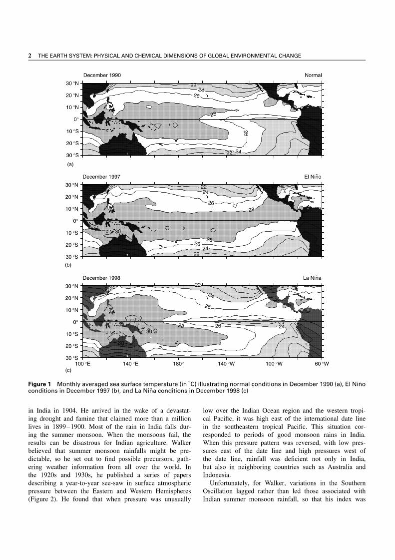
El Nino in Spanish means the child, with specific referenceto the Christ child. It was the name given by fishermento a warm southward flowing coastal ocean current thatoccurred every year around Christmas time off the westcoast of Peru and Ecuador. The term was later restricted tounusually strong warmings every few years that disruptedlocal fisheries, led to massive bird die offs, and broughttorrential rains to the region. These coastal warmings andepisodes of heavy rainfall have been linked by researchersover the past 40 years to much more extensive ocean warm-ings that occur across the width of the tropical Pacific basin(Figure 1). The term El Nino has now become synony-mous with these extensive ocean warmings because of theirimpacts on global climate (Philander, 1990).

El Nino is coupled to an atmospheric phenomenon knownas the Southern Oscillation, first defined by Sir GilbertWalker in the early 20th century. Walker was an English-man who was appointed director general of observatories

2 THE EARTH SYSTEM: PHYSICAL AND CHEMICAL DIMENSIONS OF GLOBAL ENVIRONMENTAL CHANGE

2224

26

28

26

2422

2224

26

2826

2422

28

24

24

26

2630

30

30 °N

20 °N

10 °N

0°

10 °S

20 °S

30 °S

(a)

(c)

(b)

December 1990 Normal

30 °N

20 °N

10 °N

0°

10 °S

20 °S

30 °S

December 1997 El Nino

30 °N

20 °N

10 °N

0°

10 °S

20 °S

30 °S100 °E 140 °E 180° 140 °W 100 °W 60 °W

December 1998 La Nina

22

~

~

28

Figure 1 Monthly averaged sea surface temperature (in °C) illustrating normal conditions in December 1990 (a), El Ninoconditions in December 1997 (b), and La Nina conditions in December 1998 (c)

in India in 1904. He arrived in the wake of a devastat-ing drought and famine that claimed more than a millionlives in 1899–1900. Most of the rain in India falls dur-ing the summer monsoon. When the monsoons fail, theresults can be disastrous for Indian agriculture. Walkerbelieved that summer monsoon rainfalls might be pre-dictable, so he set out to find possible precursors, gath-ering weather information from all over the world. Inthe 1920s and 1930s, he published a series of papersdescribing a year-to-year see-saw in surface atmosphericpressure between the Eastern and Western Hemispheres(Figure 2). He found that when pressure was unusually

low over the Indian Ocean region and the western tropi-cal Pacific, it was high east of the international date linein the southeastern tropical Pacific. This situation cor-responded to periods of good monsoon rains in India.When this pressure pattern was reversed, with low pres-sures east of the date line and high pressures west ofthe date line, rainfall was deficient not only in India,but also in neighboring countries such as Australia andIndonesia.

Unfortunately, for Walker, variations in the SouthernOscillation lagged rather than led those associated withIndian summer monsoon rainfall, so that his index was

EL NINO AND LA NINA: CAUSES AND GLOBAL CONSEQUENCES 3

2

2

20

–2

–2

202

2

0

–2

20

–2

L

L

0–2

–2

2

0

L

0

80°N

60°

40°

20°

0°

20°

40°

60°S

0

20 °W 20 °E 60° 100° 140° 180° 140° 100° 60 °W

L

L

–4

L

4

H8

–4

–8

–6

0

–5H

6

2

Figure 2 Spatial pattern of annual mean sea level pressure anomalies associated with the Southern Oscillation. Solidcross hatching indicates regions where sea level pressure varies in phase with Darwin, Northern Australia, and lightshading indicates regions where sea level pressure varies out of phase with Darwin. Units are in correlation coefficient(ð10), for which large absolute values indicate a more consistent relationship with Darwin (Trenberth and Shea, 1987)

−1

−3

−2

−1

0

1

2

1

2

3

0

Southern oscillation index

(a)

(b)

Temperature anomalies(5 °N−5 °S, 90 °W−150 °W)

1900 1920 1940 1960

Year

1980 2000

Tem

pera

ture

(°C

)S

tandard

devia

tion

Figure 3 (a) SOI, which is a normalized difference between Tahiti, French Polynesia minus Darwin, Australia surfaceair pressure, after typical seasonal variations have been subtracted out. Periods of SOI greater in magnitude than 0.5are shaded to emphasize the relationship with El Nino and La Nina episodes. Low SOI is associated with warm seatemperatures (El Nino), and high SOI with cold sea temperatures (La Nina). (b) Sea surface temperature anomalies (thatis, deviations from normal) for the region 5 °N–5 °S, 90 °W–150 °W from 1900–1999. Positive anomalies greater thanabout 0.5 °C indicate El Nino events. Negative anomalies less than about �0.5 °C indicate La Nina events


not useful for monsoon predictions. Curiously, he alsofound that the low index phase of the Southern Oscillationwas correlated with warm winters over Canada and dryconditions in parts of South Africa. His work was met witha great deal of skepticism though because he could notprovide a physical explanation for the observed connectionsbetween the Southern Oscillation and climatic variations inwidely separated parts of the globe. This skepticism wasevident in his obituary, published in the Quarterly Journalof the Royal Meteorological Society (1959, p. 185):

Walker’s hope was presumably not only to unearth relationsuseful for forecasting but to discover sufficient and sufficientlyimportant relations to provide a productive starting point fora theory of world weather. It hardly seems to be working outlike that.

Ironically, Walker died in 1958 during the 1957–1958International Geophysical Year (IGY), the first truly interna-tional scientific study of the global oceans, atmosphere, andsolid earth (see IGY (International Geophysical Year),Volume 1). Intensive measurements were being undertakenin a coordinated effort to better understand the processesinvolved in shaping the global environment. As fate wouldhave it, 1957–1958 coincided with a strong El Ninoevent. Measurements from the various observing systemsdeployed during the IGY stimulated Jacob Bjerknes to

examine how interactions between the ocean and the atmo-sphere in the tropical Pacific could affect weather patterns(see Bjerknes, Jacob, Volume 1). Bjerknes was a Norwe-gian meteorologist who emigrated to the US just beforeWorld War II. He had established his reputation in the earlypart of the century by making fundamental contributions tothe understanding of fronts and weather systems at middleand high latitudes. Using IGY data in the 1960s, Bjerk-nes would be the first to identify the relationship betweenEl Nino and the Southern Oscillation, to propose physicalmechanisms by which they might interact, and to describesome of the effects of El Nino on North American weather.

The close connection between El Nino and the SouthernOscillation over the past 100 years can be seen in the stronginverse relationship between two commonly used indicators(Figure 3). The Southern Oscillation index (SOI) is basedon departures from normal of surface atmospheric pressureat Tahiti, French Polynesia, and Darwin, Northern Australia.The difference of Tahiti minus Darwin pressure provides ameasure of the pressure force that drives the trade windsacross the Pacific basin. When this index is negative (lowpressure at Tahiti relative to Darwin), the trade winds areweak. When the index is positive, the trade winds arestrong.

A commonly used index for El Nino is the areal averagedsea surface anomaly (i.e., deviation from normal) in the

Box 1 El Nino and La Nina, Past and Present

El Nino and La Nina events generally last 12–18 months,and tend to be most fully developed during the North-ern Hemisphere winter season. Thus, they often spantwo calendar years. Commonly used indices like thosein Figure 3 show that El Nino events over the past50 years occurred in 1951, 1953, 1957–1958, 1963,1965–1966, 1969, 1972–1973, 1976–1977, 1982–1983,1986–1987, 1991–1995 and 1997–1998. La Nina eventsof the past 50 years occurred in 1949–1950, 1955–1956,1964, 1970–1971, 1973–1975, 1988–1989, 1995–1996and 1998–2000. Weak cold events also occurred in1967–1968 and 1984–1985, but these were not accom-panied by positive values of the SOI.

Instrumental records available for identifying El Ninoand La Nina years prior to the mid-19th century are verylimited. However, it has still been possible to identify ElNino events in the distant past using anecdotal historicalinformation from the reports of early explorers andsettlers in those areas bordering the Pacific where inmodern times El Nino consistently affects weather andclimate. Quinn et al. (1987) produced a chronology of ElNino events going back to 1525 using historical reports ofconditions from the coastal region and adjacent watersof northwestern South America. Their work suggests,e.g., that Francisco Pizarro’s conquest of the Incas in1531–1532 coincided with an El Nino event. Heavyrains and swollen rivers, which typically occur onlyduring El Nino years in Peru, delayed Pizarro’s advancethrough the countryside. On the other hand, the same

rains produced abundant vegetation, providing plentifulfodder for his horses, which were one of the chief tacticaladvantages (along with swords) that his small contingentof soldiers had over the natives.

Quinn (1992) extended this El Nino chronology backto 622 AD using maximum yearly Nile River flow dataat Cairo, and related historical information on Africandroughts, floods, plagues and famines. Careful recordsof Nile stream flow were kept because it formed thebasis of Egyptian agriculture for thousands of years. Thestream flow records reveal year-to-year changes that canbe related to variations in summer monsoon rains overthe highlands of Ethiopia. These rains, and the streamflows they feed, are typically reduced in El Nino years.

It is possible to extend the record of ENSO timescale variations even further back in time by developingclimate reconstructions using proxy data from treerings, laminated lake sediments, glacier ice cores andtropical Pacific corals. These proxies preserve year-by-year records of environmental parameters related tophysical climate, such as temperature, precipitation, orrainwater runoff. The relevant climate information isencoded in the chemical and isotopic composition ofcoral skeletons, the water content and chemistry ofice cores, the thickness and grain sizes of sedimentlayers, and the thickness and density of tree rings.Properly calibrated against modern instrumental records,proxy data allow investigations on ENSO-related climatevariability to extend many thousands of years into thepast.


region 5 °N to 5 °S, 90 °W to 150 °W. Large positive valuesof this index define warm El Nino conditions, while largenegative values indicate cold La Nina conditions. It isevident that the warm surface temperatures are stronglylinked to weak trade wind (negative values of the SOI)and vice versa. These indices show that the 1982–1983 ElNino and the 1997–1998 El Nino were the strongest of the20th century.

El Nino events exhibit some common characteristics(such as unusually warm sea surface temperatures andweak trade winds in the tropical Pacific) that allow themto be classified as a distinct phenomenon (see Box 1).However, they often differ among themselves in dura-tion, intensity and in the details of their development.No two El Ninos are exactly alike, and the same is trueof La Nina events. Thus, the ENSO cycle displays adegree of irregularity for which there is yet no simpleexplanation.

EL NINO PHYSICS AND THE ENSO CYCLE

To understand El Nino, we must first understand what isconsidered normal. Sunlight reaching the Earth’s surface ismore intense in the tropics than at higher latitudes, so thatthe warmest ocean temperatures are found near the equa-tor. Air masses over warm tropical waters extract heat andmoisture from the ocean, expand, become less dense thansurrounding air, and ascend to higher altitudes. The ris-ing air cools and condenses, producing towering cumulusclouds and heavy precipitation through a process referred toas deep convection. At upper levels of the troposphere (thelowest 10–12 km of the atmosphere affected by weather)these air masses flow poleward, then sink in regions of highsurface pressure over the subtropical oceans of the Northernand Southern Hemispheres. The rising tropical air massesin turn are fed by air drawn in towards the equator near thesurface from the subtropical high-pressure zones. This cir-culation cell on the meridional plane is called the Hadleycirculation in honor of George Hadley, an 18th centuryBritish meteorologist who was the first to provide a theoret-ical explanation for it (see Hadley Circulation, Volume 1).

The equatorward flowing surface air masses are deflectedwestward because of the rotation of the Earth about itsaxis (the Coriolis effect). The result is easterly tradewindsystems in the Northern and Southern Hemispheres. Thenortheast and southeast trade winds meet in the Intertropi-cal Convergence Zone, situated on average about five to tendegrees of latitude north of the equator in the Pacific. This isa region of deep convection, cumulus cloud formation, andheavy rainfall that comprises the ascending branch of theHadley circulation. A second zone of converging surfacewinds, the South Pacific Convergence Zone, is on averagelocated several degrees south of the equator in the westerntropical Pacific.

Normal conditions

Walker circulation

Thermocline

Thermocline

80 °W120 °E

El Niño conditions

Equator

80 °W120 °E

Equator

Figure 4 Schematic of normal and El Nino conditions inthe equatorial Pacific

Along the equator, the trade winds normally drive surfaceflow westward in the south equatorial current (Figure 4).This current piles up the warm surface water in the westernPacific, and drains it from the eastern Pacific. The ther-mocline, which is the sharp vertical temperature gradientseparating the warm surface layer from the cold deep ocean,is pushed down to a depth of 150 m in the west, but shoalsto 50 m depth in the east. Sea level tends to mirror thermo-cline depth since water expands when heated. Thus, whilethe thermocline tilts downward towards the west along theequator, sea level rises to the west where it stands about60 cm higher than in the eastern Pacific.

The relative shallowness of the thermocline in the east-ern Pacific facilitates the upward transport of cold interiorwater by the trade winds, and a cold tongue develops insea surface temperature from the coast of South Americato near the international date line. The east–west surfacetemperature contrast reinforces the easterly trade winds,since low atmospheric surface pressure is associated withwarm water in the west and high surface pressure with


Box 2 Equatorial Waves

One early theory for El Nino postulated that the windsblowing equatorward off the west coast of SouthAmerica weakened during an El Nino event, so thatcoastal upwelling would be reduced and sea surfacetemperatures would rise. However, Klaus Wyrtki, anoceanographer at the University of Hawaii, demonstratedin the mid-1970s that winds along the coast of SouthAmerica actually strengthened during El Nino (Wyrtki,1975). He found instead that weakening of the tradewindsthousands of kilometers to the west in the centralPacific was related to the development of El Ninoalong the coast of South America some months later.Based on these results, Wyrtki suggested that large scaleequatorial ocean waves were the mechanism by whichwind variations in the central Pacific could lead to theonset of El Nino in the eastern Pacific.

Two classes of oceanic waves are important forunderstanding the cycle of El Nino and La Nina variations.One class is referred to as Kelvin waves, namedafter Lord Kelvin (William Thompson), a 19th centuryBritish physicist who was the first to theoreticallypredict such waves in rotating fluids. The other classis referred to as Rossby waves, named after Carl-Gustaf Rossby, a Swedish-born meteorologist who in

the 1930s first discovered this kind of wave in theatmosphere (see Rossby Waves, Volume 1; Rossby, Carl-Gustaf, Volume 1). Both types of wave are generated inthe equatorial ocean by large-scale variations in surfacewinds.

Kelvin waves propagate eastward along the equatorand Rossby waves propagate westward. They are evidentbelow the surface as undulations of the thermocline,causing it to rise and fall by tens of meters as the wavespass by. Equatorial waves also affect sea level and theintensity and direction of ocean currents. The Earth’srotational forces trap these waves within several hundredkilometers of the equator in the open ocean, so theytransfer energy very efficiently over many thousands ofkilometers in the east–west direction.

Kelvin waves take about two months to cross thePacific basin and Rossby waves take about six monthsto cross. When they reach the landmasses at the easternand western boundaries of the ocean, they reflect backinto the interior and, in the case of Kelvin waves, leakenergy to higher latitudes along the west coasts ofthe Americas. The life cycle of these waves, evolvingover many months and seasons in response to changingwinds, are a critical aspect of ocean dynamics controllingthe evolution of El Nina and La Nina events.

cooler water in the east. Also, as the trade winds flowfrom east to west, they pick up heat and moisture fromthe ocean. The warm, humid air mass becomes less denseand rises over the western Pacific warm pool where deepconvection leads to towering cumulus clouds and heavyprecipitation. Ascending air masses in this region of deepconvection return eastward in the upper levels of the tro-posphere, then sink over the cooler water of the EasternPacific. Bjerknes labeled this atmospheric circulation pat-tern on the equatorial plane the Walker circulation inhonor of Sir Gilbert Walker (see Walker Circulation, Vol-ume 1).

Upwelling is a key oceanic process that regulates seasurface temperatures along the equator and along muchof the west coast of the Americas. Wind-driven surfacecurrents flow to the right of the winds in the NorthernHemisphere and to the left of the winds in the SouthernHemisphere because of the Coriolis force. Easterly tradewind-driven currents therefore flow poleward in oppositedirections near the equator in the Northern and SouthernHemispheres. This divergent surface flow is fed from belowby upwelled thermocline water to create the equatorial coldtongue (Figure 1). A similar process operates off the westcoasts of the Americas. Equatorward winds on the easternflanks of subtropical high-pressure systems drive surfacewaters offshore. These offshore flows are fed from belowby cooler thermocline waters, which then lower coastal seasurface temperatures.

During El Nino, the trade winds weaken in the westernand central equatorial Pacific as atmospheric pressure rises

in the west and falls in the east (Figure 4). Weakened tradewinds generate waves in the ocean interior, which radiatealong the equator both to the east and to the west away fromthe region of wind forcing (see Box 2). Over the course ofa few months, these waves elevate the thermocline in thewest and push it down in the east. In the cold tongue region,depression of the thermocline leads to surface warming asequatorial upwelling can no longer efficiently tap into thecold water reservoir below. Westward flow in the southequatorial current also weakens and reverses when the tradewinds relax, allowing the western Pacific warm pool tomigrate eastward. Sea level drops in the west and rises inthe east in response to the redistribution of warm surfacewaters.

As sea surface temperatures warm east of the date line,the pattern of deep convection and precipitation also shiftseastward. This reinforces the reduction in trade wind inten-sity, because westerly winds flow into the convective centerfrom the west. Pressure continues to fall in the east and risein the west as the region of convection and rainfall migrateseastward. The system becomes locked in a positive feedbackloop, with warming surface temperatures leading to weak-ened trade winds and vice versa. This positive feedback iseventually broken when the oceanic waves that elevated thethermocline in the western Pacific at the onset of the eventbounce off the land masses bordering the western Pacific andreflect back toward the east. As the reflected waves propagateeastward along the equator, they elevate the thermocline andinitiate surface cooling. Cooler surface waters in the easternPacific increase the east–west atmospheric pressure gradient


and the strength of the trade winds, which in turn reinforcessurface cooling through intensified upwelling. These inter-actions between the ocean and the atmosphere terminateEl Nino typically 12–18 months after its onset. The oceanreturns to near normal conditions, or it may overshoot into acold La Nina state.

While El Nino involves an intimate coupling of the atmo-sphere and the ocean, the two fluids respond to each otheron very different time scales. The atmosphere is a thousandtimes less dense than the ocean, and therefore respondsalmost immediately to forcing from the ocean surface. Theocean is massive by comparison, so its dynamical responseto atmospheric forcing is relatively sluggish. For example,thermocline depths may take many months to adjust tochanging winds in the tropics, whereas atmospheric con-vection can develop within hours over warm surface water.It is the slow evolution of the upper ocean thermal field thatprovides the memory for the climate system in the tropicalPacific, and it is this thermal inertia that provides the basisfor predictability of ENSO time scale variations.

EL NINO WEATHER IMPACTS

One impact of the eastward shift in rainfall along theequator during El Nino is that drought develops in Aus-tralia, Indonesia and neighboring countries. On the otherhand, the island states of the central Pacific and the westcoast of South America are inundated with heavy rains.Heavy rainfall bands normally situated north and south ofthe equator in the Intertropical Convergence Zone and theSouth Pacific Convergence Zone also shift equatorward assurface waters warm. These latitudinal shifts contribute tounusually heavy rains near the equator in the central andeastern Pacific, and to drought conditions at higher latitudesin regions such as New Caledonia and Fiji to the south, andHawaii to the north.

Heat released into the troposphere from deep tropicalconvection is one of the principal driving forces for theglobal atmospheric circulation. Changes in the locationof tropical heat sources during El Nino therefore lead towidespread changes in wind and weather patterns outside

L

H

L

H

H

L

140 °W160 °W

180 °W100 °W

120 °W

NP

Equator

0

0

0

10 °N

30 °N

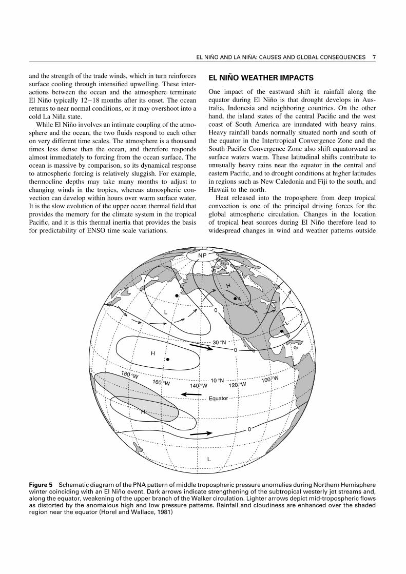
Figure 5 Schematic diagram of the PNA pattern of middle tropospheric pressure anomalies during Northern Hemispherewinter coinciding with an El Nino event. Dark arrows indicate strengthening of the subtropical westerly jet streams and,along the equator, weakening of the upper branch of the Walker circulation. Lighter arrows depict mid-tropospheric flowsas distorted by the anomalous high and low pressure patterns. Rainfall and cloudiness are enhanced over the shadedregion near the equator (Horel and Wallace, 1981)


the tropical Pacific. These remote effects of El Nino arereferred to as teleconnections. In the extratropics, telecon-nections are usually most pronounced during the winterseason, though they are detectable in other seasons as well.

Anomalous tropospheric heating in the central tropicalPacific during El Nino generates quasi-stationary atmo-spheric wave trains that radiate poleward and eastward.In the Northern Hemisphere, these waves set up thePacific North American Teleconnection Pattern, or (PNA)pattern, which is a series of high- and low-pressure cen-ters extending from the central North Pacific to NorthAmerica (Figure 5). During El Nino, the Aleutian low pres-sure center over the North Pacific deepens, high pressuredevelops over western North America, and low pressureprevails over the southeastern US. These pressure changessteer warmer air masses from southern latitudes into the

Pacific Northwest and southern Canada, so that much ofCanada and the northwestern US tend to experience mildwinters. Low pressure in the southeastern US associatedwith the PNA pattern brings wetter, cooler conditions to thestates bordering the Gulf of Mexico. Similar wave trains areexcited in the Southern Hemisphere, but they are weakerand more variable than those in the north.

Teleconnections also affect the subtropical jet streamswhich are swift air flows girdling the Earth at altitudescentered between about 10 000 m and 12 000 m (see Tele-connection, Volume 1). The eastward migration of deepconvection during El Nino causes the core of these jetstreams to intensify and shift southeastward in the centraland eastern Pacific (Figure 5). The jet streams are a majorinfluence on the location of storm tracks, so that southernCalifornia and northern Chile typically experience stormier

Dry&

Warm

El Niño weather patterns June–August

El Niño weather patterns December–February

Wet & Warm

Wet

WarmWarm

Wet & Cool

Warm

Wet

Dry

DryWarm

Wet

Warm

Dry

Warm

Wet

WetWet

Warm

Dry

Dry

Wet

Warm

Dry & Warm

Dry & CoolDry

60 °E 120 °E 180° 120 °W 60 °W

70 °N

50 °N

30 °N

10 °N

10 °S

30 °S

50 °S

70 °N

50 °N

30 °N

10 °N

10 °S

30 °S

50 °S

0°

60 °E 120 °E 180° 120 °W 60 °W0°

Figure 6 Schematic diagram showing temperature and precipitation anomalies associated with El Nino. To a firstapproximation, the impacts of La Nina are similar, but with opposite sign (Ropelewski and Halpert, 1987 and Halpert andRopelewski, 1992)


and wetter weather in their respective winter seasons duringEl Nino.

Teleconnections affect surface conditions over landmasses and the ocean. At extratropical latitudes of the Northand South Pacific, for example, sea surface temperaturescool in response to intensified surface wintertime westerlies.Over land, changes in temperature and precipitation canaffect soil moisture and evapotranspiration. These changesin surface conditions can feed back to the atmosphere,affecting the overall climatic response to El Nino forcing.

A global composite of typical rainfall and air temperatureanomalies associated with El Nino is presented in Figure 6.In addition to effects already mentioned, El Nino yearsgenerally bring drought in northeastern Brazil, southernAfrica, and the western Pacific, and wetter conditions tosouthern Brazil, Uruguay, Peru, and equatorial East Africa(Ropelewski and Halpert, 1987). Indian monsoon summerrains tend to be weaker during El Nino events, consistentwith the strong relation between the Southern Oscillationand Indian monsoon rainfall noted by Walker.

El Nino also affects tropical storm frequency, intensity,and spatial distribution (Gray, 1984). In the Atlantic, 10named tropical storms, of which six reach hurricane inten-sity (wind speeds greater than 33 ms�1), form during a typi-cal June to November hurricane season. However, during ElNino, an intensified subtropical jet stream shears off the topof fledgling storms before they fully develop. Thus, fewertropical storms and hurricanes form, and those that do formtend to be weaker and shorter lived. The summer of 1997was a particularly striking example of reduced Atlantic hur-ricane activity during El Nino. Only seven named stormsformed, three of which reached hurricane intensity.

Intense tropical storms in other regions (referred to ashurricanes in the northeastern Pacific, typhoons in the north-western Pacific, and cyclones in the Indian ocean andSouthern Hemisphere) are affected more in terms of theirspatial distribution and intensity than in terms of totalnumbers (see Hurricanes, Typhoons and other TropicalStorms – Descriptive Overview, Volume 1; Hurricanes,Typhoons and other Tropical Storms – Dynamics andIntensity, Volume 1). Heat from the underlying ocean sur-face is a major source of energy for intense tropical storms,which are almost always generated over waters warmerthan 26 °C. Therefore, extensive warming of the easternPacific during El Nino allows hurricanes to travel fartherwestward and northward and, in some cases, attain greaterstrength. Similarly, the eastward extension of warm tropicalsurface waters along the equator during El Nino expandsthe area over which typhoons and cyclones may spawn.Changes that can occur in tropical storm activity in theeastern Pacific during El Nino are exemplified by the 1997season when hurricane Linda grew to record strength andhurricane Nora tracked far to the north, bringing heavy rainsto normally arid northern Mexico and the southwestern US.

In the South Pacific during the 1982–1883 El Nino, oceansurface warming allowed six cyclones to strike French Poly-nesia, a region not usually prone to experiencing intensetropical storms (Canby, 1984).

El Nino affects the coastal zones of the Americas all theway to Alaska in the Northern Hemisphere and at least tocentral Chile in the Southern Hemisphere. When eastwardpropagating oceanic waves generated by weakening of thetrade winds at the onset of El Nino reach the coast ofSouth America, part of the wave energy is reflected backinto the open ocean, but part also radiates northward andsouthward along the coasts. The coastal waves push thethermocline down and reduce the upwelling of cool wateras they progress poleward. Within one to two months afterthe first equatorial waves reach South America, sea sur-face temperatures rise all along the coast to the north andsouth. North of central California, southerly surface windsrelated to the PNA pattern also contribute to coastal warm-ing (Ramp et al., 1997). These winds both bring warmsubtropical air northward, and also drive on-shore oceancurrents that converge at the coast to push the thermoclinedown.

The unusually thick layer of warm surface water alongthe west coast causes near shore sea levels to rise by15–30 cm during El Nino. In addition, offshore win-ter storms associated with intensified jet streams in thesubtropics can generate unusually high ocean swells andstorm surges in coastal zones. Storm-generated surfacewaves and currents, and high tides, can add to already ele-vated sea levels high tides to cause severe coastal erosion.In communities with major shoreline development such asin southern California, the combined assault from high seasand heavy rains can lead to significant loss of propertyand life.

The impacts of El Nino on weather are most consistentfrom event to event in the tropical Pacific and border-ing areas. Impacts are prominent, but less consistent, athigher latitudes and in other ocean basins where regionalinfluences can become important. Thus, although El Ninoincreases the probability of a particular kind of weatherpattern occurring in particular regions of the globe, actualimpacts may vary from those expected for any given event(Trenberth et al., 1998).

ECOSYSTEMS IMPACTS

Narrow coastal and equatorial upwelling zones account formuch of the biological productivity in the world’s oceans.One-celled plants known as phytoplankton are at the baseof the aquatic food chain in these regions, and all higherorganisms depend directly or indirectly on them as a foodsource. Upwelling ecosystems are rich in species diversityand abundance, including many types of phytoplankton,zooplankton, shellfish, crustaceans, fish, marine mammals,


and sea birds. Many of the fish and shellfish species suchas tuna, anchoveta, sardines, squid, and shrimp are valuablecommercially.

Primary productivity is the rate at which carbon is takenup by phytoplankton via photosynthesis. Nutrient limitationcontrols primary productivity in tropical and subtropicalregions where sunlight is plentiful. The principal sourcefor nutrients, away from river outflows and areas of signifi-cant coastal runoff, is the thermocline. Small organisms thathave died near the surface decay and remineralize as theyslowly sink out of the euphotic zone (the well lit upperlayer of the ocean). Fecal pellets from larger organismslikewise sink and decompose at depth. These processescreate a pool of nutrients and remineralized carbon inthe thermocline which, when upwelled into the euphoticzone, are available for uptake by phytoplankton. Lateralflows in the thermocline may bring nutrients and carbonfrom great distances before they are upwelled, concentrat-ing primary production in narrow equatorial and coastalzones.

During El Nino, ocean dynamical processes depress thethermocline in the eastern and central equatorial Pacific,and along the coasts of North and South America. Thesupply of nutrients to the euphotic zone drops or maybe cut off entirely. Primary production decreases, witheffects that ripple through the entire food chain (Barberand Chavez, 1984). Zooplankton that feed on phytoplank-ton decrease in abundance. Fish, sea birds and marinemammals die off or migrate to more productive regionsin search of food. Undernourished sea birds and marinemammals may experience reproductive failures or abandonyoung when food becomes scarce. In extreme cases, deci-mated populations may require one or more years to fullyrebound.

El Nino can also cause bleaching of tropical corals whenwater temperatures become too warm (Strong et al., 2000)(see Coral Reefs: an Ecosystem Subject to MultipleEnvironmental Threats, Volume 2 and Coral Bleaching(1997–1998), Volume 2). Corals thrive in a narrow range oftemperatures between about 18 and 28 °C. At temperaturesabove the upper threshold, they expel symbiotic algae thatreside in their polyps. The algae add color to healthy corals,and their metabolic by-products are essential for coralsurvival. Coral can recover from bleaching unless watertemperatures remain too high for too long. The concernover lethal bleaching is that it threatens the vitality of coralreef ecosystems, which support local fisheries and providetourist income. Massive and widespread coral bleachingoccurred during 1998 in the Galapagos Islands, off thecoast of Panama, in the Great Barrier Reef of Australia andelsewhere in the tropics in response to the exceptionallystrong 1997–1998 El Nino. Decadal warming trends intropical ocean temperatures contributed to this bleaching,by elevating background temperatures on which El Nino

warming was superimposed. These decadal trends, possiblyrelated to global warming, have raised concerns aboutprolonged deterioration in the health of coral reefs.

El Nino can also dramatically affect fisheries, a partic-ularly striking example of which was the collapse of thePeruvian anchoveta fishery following the 1972–1973 ElNino (Glantz, 2001). In the late 1960s and early 1970s,Peru was the most productive fishing nation in the world.The annual catch of anchoveta was over 10 million metrictons, one fifth of the global total. Most of the catch wasexported for use as a feed supplement in poultry farms, withthe exports accounting for nearly one third of Peru’s foreignexchange earnings. Concerns were voiced at the time thatoverfishing might be depleting the stocks from sustain-able levels. Those concerns proved to be well founded.Intense fishing pressure and extraordinarily high mortalityrates during the 1972–1973 El Nino caused the fishery tocrash. Effects were long lasting. For at least 10 years fol-lowing the 1972–1973 El Nino, anchoveta landings rangedbetween only 1/10–1/3 the catch of 1970.

It was the collapse of the Peruvian anchoveta fisherythat focused international attention on the socio-economicconsequences of El Nino. A reduction in the supply offishmeal caused many farmers in the US to switch fromplanting wheat to planting soybeans. Soy is an alternativesource of poultry feed supplement and more lucrative thanwheat as a cash crop. However, wheat harvests had declinedin many nations, particularly the Soviet Union, becauseof widespread droughts in 1972. Staple food shortagesdeveloped in some regions and prices steeply increasedfor basic commodities in others. These events highlightedthe role of climate in affecting global economies, andspecifically focused attention on the need for a betterunderstanding of the El Nino phenomenon.

DEVELOPMENT OF ENSO OBSERVING ANDFORECASTING SYSTEMS

Research efforts in both oceanography and meteorologyin the decade following the 1972–1973 El Nino gath-ered momentum, motivated by heightened awareness ofEl Nino’s global socio-economic consequences, and theprospect that it might be predictable. It was recognized thatadvance warning of an impending El Nino would poten-tially be extremely valuable for either disaster preparednessor for exploiting opportunities created by altered environ-mental conditions. Thus, in the early 1980s, the interna-tional research community began mobilizing resources fora major 10-year study of El Nino. This study, called theTropical Ocean-Global Atmosphere study, or (TOGA), tookplace from 1985–1994.

The 1982–1983 El Nino, the strongest in over 100 years,occurred as plans for TOGA were being formulated. ThisEl Nino left a global swath of devastation in its wake. It had


not been predicted because El Nino forecasting capabilitieshad not yet been developed. Even more stunning to theresearch community, however, was that it was not evendetected until nearly at its peak. At the time, most oceano-graphic data were available for analysis only months, or insome cases years, after they had been collected. A handfulof scattered but more readily available ocean and weatherdata from islands and volunteer observing ships suggestedthe development of unusually warm conditions in mid-1982, but these reports were discounted as erroneous. Onereason was that the 1982–1983 El Nino developed dif-ferently than expected from conventional wisdom. Therehad been no prior strengthening of the trade winds, and nowarming off the west coast of South America in early 1982,both considered at the time to be necessary precursors ofan impending El Nino. To complicate matters, eruptionsof the Mexican volcano El Chichon in March–April 1982

injected a massive cloud of aerosols (dust, soot, and otherfine particles) into the lower stratosphere, where prevail-ing winds spread it around the globe at low latitudes withinweeks. This cloud of volcanic aerosols produced undetectedcold biases of several degrees Celsius in satellite measure-ments of sea surface temperature. It was only after definitivereports were received from a research cruise in the easternequatorial Pacific that the scientific community realized towhat extent existing data sources and simplistic notions ofEl Nino evolution had misled them.

The lessons from this experience were clear: there wasurgent need for improved monitoring, detection, and under-standing of El Nino, as well as an urgent need to developreliable El Nino forecast models. Observational require-ments were met in part by utilizing data from a constel-lation of satellites viewing the Earth from space. However,satellites require Earth-based measurements for calibration

Moored buoys

Volu

nt

eer observing

ships

Drifting buoys

Tide gage stations S

atellite data relay

Figure 7 The ENSO Observing System. The four major elements of this observing system are; (1) a volunteer observingship program for surface marine meteorological observations and ocean temperature profiles (shown by schematic shiptracks); (2) an island and coastal tide gauge network for sea level measurements (circles); (3) a drifting buoy networkfor sea surface temperatures and ocean currents (shown schematically by curved arrows); (4) a moored buoy array forwind, ocean temperature, and ocean current measurements (squares and diamonds). Thick ship tracks indicate repeattransects 11 or more times per year; thin ship track indicate repeat transects six to ten times per year. One schematicdrifting buoy arrow represents 10 actual randomly distributed drifters (McPhaden et al., 1998)


and verification. Also, satellites do not see below the oceansurface, where critical oceanic processes operate to produceEl Nino events. An ocean observing system specificallydesigned for El Nino was therefore developed under theauspices of the TOGA program (McPhaden et al., 1998)(see TOGA (Tropical Ocean Global Atmosphere), Vol-ume 1). It included an extensive network of moored buoys,drifting buoys, volunteer observing ships, and tide gauges(Figure 7). One of the most important attributes of thissystem was that most of the data were transmitted via satel-lite relay to shore stations within hours of collection. Theobserving system was implemented through an internationalcollaborative effort spanning the full 10 years of TOGA,and was completed only in the last month of the program(December 1994). Continued after TOGA, it is now calledthe ENSO Observing System. The 1997–1998 El Nino wasthe first for which the ENSO Observing System was in placefrom start to finish, so that this event was not only amongthe strongest on record, but also the best ever documented(McPhaden, 1999).

Progress in the development of the ENSO ObservingSystem has been paralleled in the development of ENSOforecast models (National Research Council, 1996). Thesemodels range from statistical approaches based on the aver-age behavior of previous ENSO variations, to complexdynamical models that explicitly represent the physical pro-cesses at work in the coupled ocean-atmosphere system.The 1986–1987 El Nino was the first to be successfully pre-dicted with these techniques, which have since undergonecontinual refinement and improvement. As one measure ofsuccess, many ENSO forecast models predicted that 1997would be unusually warm in the tropical Pacific at least oneto three seasons in advance (Barnston et al., 1999). Long-range weather forecasting schemes that included informa-tion about tropical Pacific conditions during the 1997–1998El Nino likewise had success in predicting surface air tem-perature and precipitation patterns in widely disparate partsof the globe months in advance. For instance, the forecastfor wintertime precipitation and temperature issued by theNational Centers for Environmental Prediction in Washing-ton, DC, in the fall of 1997 were among the most accurateever for the continental US.

Successful seasonal forecasts, unprecedented high def-inition ocean measurements from the ENSO ObservingSystem, and record warmth in the tropical Pacific all com-bined to capture the attention of the public in 1997–1998.Media coverage was so intense that El Nino became ahousehold word all over the world. As a result of the height-ened public awareness about El Nino and its consequences,many individuals, municipalities, businesses, and in somecases national governments mobilized resources in an effortto prepare for El Nino’s onslaught. It is likely that withoutthe advance warning made possible by new measurement

and forecasting capabilities, the toll in terms of lives, prop-erty damage, and economic losses due to the 1997–1998El Nino would have been much higher.

SOCIO-ECONOMIC IMPACTS OF THE1997–1998 EL NINO

The 1997–1998 El Nino affected the lives of tens ofmillions of people around the globe. Significant disrup-tions were experienced in agriculture, forestry, fisheries,transportation, communications, power generation, publichealth and other climate-sensitive areas of human endeavor.Weather-related disasters and disease outbreaks duringthis El Nino claimed over 22 000 lives worldwide andcaused US$36 billion dollars in economic losses (Sponberg,1999).

The 1997–1998 El Nino brought torrential rainfallsand flooding to parts of California, the southeastern US,equatorial East Africa and Chile. It was also responsi-ble for severe droughts in Papua New Guinea, Indonesia,Central America, and northeastern Brazil (Supplee, 1999;WMO, 1999). Many regions experienced extensive cropfailures and livestock losses due to these droughts andfloods. Life-threatening food and drinking water short-ages developed in New Guinea, prompting internationalrelief efforts. In some drought-stricken regions, forest firesraged for months, devastating the countryside. The droughtand fires in Indonesia produced deadly smog that coveredan area one half the size of the continental US, causingwidespread respiratory ailments, and contributing to air-line and shipping disasters. Unusually low water levels inthe lakes that feed the Panama Canal forced officials torestrict traffic through the waterway for the first time in15 years.

Flood-contaminated water supplies in some regions con-tributed to outbreaks of cholera and dysentery. Stagnantpools of floodwater also provided ideal breeding groundsfor mosquitos and other insects that spread infectious dis-eases like malaria and dengue fever. Public health emer-gencies developed in Southeast Asia, South America, andAfrica as these diseases afflicted thousands of people.

Heavy rains and flooding from El Nino damaged ordestroyed roads, bridges, buildings and phone and powerlines in many parts of the globe. Thousands of individ-uals and families lost homes and personal property dueto storms, floods, mud slides and land slides. Hydroelec-tric energy generation was curtailed in regions of severelyreduced rainfall and stream flow. Many business lostincome as a result of weather-related closures, commodityshortages or shifts in market demand for consumer goods.Tourism was affected because of extreme weather in areassuch as southern California and Florida. The catch of Peru-vian anchoveta fell sharply as in previous El Nino years,and the fishery was briefly closed by government decree


as a precautionary measure to limit further depletion ofthe remaining stock. Economic hardship followed severedeclines in catch experienced in three of the four majorfisheries (tuna, squid, sardine) off the west coast of BajaCalifornia.

Despite losses of life, property, and income, 1997–1998El Nino produced some benefits as well (Changnon, 1999).Losses from Atlantic hurricanes were greatly reduced, asonly one of three hurricanes that formed made landfall.Parts of the US Midwest and the Great Lakes regionexperienced the mildest winter in over 100 years, as tem-peratures warmed to record highs between November 1997and February 1998. The milder than normal winter reducedheating bills, weather-related travel delays for the trans-portation industry, and deaths from exposure. It has beenestimated that for the US as a whole, the 1997–1998 ElNino produced a net economic gain of about $16 billiondollars and resulted in 650 fewer deaths than would haveotherwise occurred.

Similarly, not all fisheries were hit hard by the1997–1998 El Nino. Though severe declines in mostcommercial fisheries were experienced off the west coast ofBaja California, these declines were partially offset by aneight-fold increase in the catch of more lucrative shrimp.Likewise, shrimp catch increased off the coast of Ecuador,with export revenues rising by 40% in 1997 (WMO, 1999).Northward migration of warm water fish species such asmarlin, tuna and mahi-mahi was also a boom to the sport-fishing industry off the west coast of the US.

The 1997–1998 El Nino highlighted societal sensitivi-ties and vulnerabilities to year-to-year climate fluctuationson a global scale. It also demonstrated that losses andgains are inherently unevenly distributed across economicsectors and national boundaries. Spurred in part by thedramatic consequences of this El Nino, new areas of inter-disciplinary research are emerging to examine the use ofEl Nino-related climate information in economic planningand policy decisions. These efforts involve both social andphysical scientists, with a focus on not only how forecastsare generated, but also how they are disseminated, inter-preted, and acted upon.

LA NINA

La Nina is the cold phase of the ENSO cycle (Philander,1990). It is characterized by stronger than normal tradewinds, colder tropical Pacific sea surface temperatures,and positive values of the SOI (Figure 3). It represents asituation in which oceanic and atmospheric processes whichgive rise to normal conditions illustrated in Figure 4 areexaggerated, with deep convection and heavy rainfall alongthe equator shifted even further to the west and confined toa narrower range of longitudes. The term La Nina (the girl )was coined in the mid-1980s by scientists investigating the

year-to-year oscillations between warm and cold conditionsin the tropical Pacific. La Nina has also been referredto as anti-El Nino, ENSO cold event, and El Viejo (theold man). Like El Nino, La Nina typically lasts 12–18months.

La Nina’s effects on global weather variability areroughly (though not exactly) opposite to those of ElNino (Halpert and Ropelewski, 1992). The atmosphericresponse to weak-to-moderate cold and warm tropicalPacific sea surface temperature anomalies tends to be sim-ilar in magnitude, but opposite in sign. However, theatmospheric response to strong La Nina events tends tobe weaker than the response to strong El Nino events.This difference arises because tropical rainfall (whichtranslates into atmospheric heating and associated tele-connection patterns) has a lower limit of zero, regardlessof how cold the tropical Pacific may get. On the otherhand, the upper limit for rainfall and hence atmosphericheating during strong El Nino events is not as rigidlyconstrained.

Examples of La Nina weather impacts include anincreased probability of unusually rainy conditions insouthern Africa and northeastern Brazil, and in the monsoonregions of India, Indonesia and Northern Australia. LaNina is often linked to drier than normal conditions overequatorial East Africa, southern Brazil and Uruguay. Thesubtropical jet streams over the Pacific weaken, shiftpoleward, and become more variable in strength duringLa Nina winters. Blocking highs tend to develop in theeastern North Pacific, accompanied by more frequent coldpolar air outbreaks over western North America. Thesechanges in atmospheric pressure patterns and circulationresult in winters that tend to be colder and stormierthan normal over Alaska, western and central Canada,and the northern US. Conversely, the northward shiftin the subtropical jet stream leads to warmer and drierthan normal conditions in the southeastern US, anddrier than normal conditions in the southern plains ofthe US.

La Nina, like El Nino, affects tropical storm frequency,intensity, and geographical distribution through changes insea surface temperature and atmospheric circulation. Pacifichurricanes, typhoons and cyclones are more restricted intheir geographical extent because of colder underlying seasurface temperatures. On the other hand, Atlantic hur-ricanes tend to increase in number as the subtropicaljet stream shifts northward, reducing the shear betweenupper and lower level tropospheric winds where hurri-canes form. The 1995 Atlantic hurricane season is a goodexample of what can happen during La Nina. That yearwitnessed a bumper crop of 19 named tropical Atlanticstorms, including 11 hurricanes, almost double the usualnumber.


La Nina’s socio-economic impacts can be as impressiveas those resulting from El Nino. La Nina-related droughtand heat waves in the US Midwest during the summerof 1988 constituted one of the worst natural disasters inUS history, causing US$40 billion in agricultural and otherlosses, and claiming approximately 7500 lives from heatstress. Also, with more and stronger Atlantic hurricanesduring La Nina, their destructive potential and probabilityof making landfall in populated regions increases. For theUS, it is three times more likely that an intense hurricanewill make landfall during a La Nina than during an El Nino.Hurricane Mitch, one of the strongest Atlantic hurricanes onrecord and the deadliest in 200 years, was spawned duringthe 1998 La Nina. Mitch devastated Central America,claiming 10 000 lives, leaving over three million homeless,and causing US$6 billion in damage.

La Nina can also be beneficial to some regions ofthe globe. For instance, higher monsoon rainfall totalsover the Indian subcontinent, the western Pacific, andnortheastern Brazil can support greater agricultural pro-duction and economic growth. Enhanced winter snowpackin the mountains of the Pacific Northwest provide forextra hydroelectric power production, ample summer watersupplies, and improved freshwater habitat for salmon. Interms of marine ecosystems, primary productivity, drivenby more intense equatorial and coastal upwelling, is gener-ally enhanced. Higher-level marine organisms tend to thriveunder these conditions, and severe disruptions in fisheries,like those during El Nino, are not so evident.

DECADAL VARIATIONS AND GLOBALWARMING

The frequency and amplitude of El Nino and La Nina eventsare modulated on decadal and longer time scales. The 1930sto the early 1950s, for example, was a period of relativelyfew El Ninos, while the period since 1976 has witnessedmore frequent, stronger, and in the case of 1991–1995,longer lasting El Ninos. In addition, the magnitude of thestrongest El Ninos over the past 50 years seems to beincreasing while at the same time there has been a trendtoward fewer La Nina events (Figure 3).

Variations in the ENSO cycle may simply be a resultof random or chaotic fluctuations in the Earth’s highlycomplex climate system. However, there may be other fac-tors at work as well. Temperatures have been elevatedin the tropical Pacific since the mid-1970s in associa-tion with a recently discovered, naturally occurring phe-nomenon known as the Pacific Decadal Oscillation, or(PDO) (Mantua et al., 1997) (see Pacific–Decadal Oscilla-tion, Volume 1). This oscillation alternates between phasesof warm and cold tropical Pacific sea temperatures last-ing 20–25 years. The physical mechanisms that account

for the PDO are at present poorly understood. How-ever, the PDO affects the background oceanographic andatmospheric conditions on which ENSO events develop.Warm phase PDO and El Nino sea surface temperatureanomalies are roughly additive. Under these conditions,the global atmospheric teleconnection patterns set up byelevated tropical Pacific sea surface temperatures can beamplified.

In addition to naturally occurring phenomena such asthe PDO, global warming may also affect the ENSOcycle (Trenberth and Hoar, 1996). The warmest years onrecord were 1998 and 1997, in that order. Occurrence of1997–1998 El Nino contributed in part to these extremes,because global temperatures rise a few tenths of a degreeCelsius following the peak El Nino warming in the trop-ical Pacific. However, aside from the record warmth in1997–1998, there has been an underlying trend towardincreased globally averaged air temperatures of about 0.6 °Cover the past century. Moreover, tree ring and ice core dataindicate that the 20th century has been the warmest centuryand the 1990s has been the warmest decade over the pastmillennium. The consensus of the scientific community atpresent is that the recent increase in global temperatures ishuman-induced through fossil fuel combustion and defor-estation (Houghton et al., 1996).

It is reasonable to assume that anthropogenic greenhousegas warming will affect ENSO because both phenomenaare involved in regulating the Earth’s heat balance. Inaddition, an altered ENSO cycle may leave its imprint onthe global carbon balance (see Box 3) and on patterns ofregional climate change. If global warming were to lead tointensified, more frequent, or prolonged El Ninos, thoseregions affected by El Nino-related drought or flood inthe present climate might well be more prone to suchnatural disasters in the future. How global warming mayaffect ENSO and other natural modes of climate variabil-ity is not known at present though. Computer models usedfor developing scenarios of how the Earth’s climate willchange in response to elevated levels of carbon dioxide(CO2) and other greenhouse gases in the atmosphere differon how the tropical Pacific Ocean will be affected (Meehlet al., 2000). Many coupled ocean-atmosphere models pre-dict a permanent El Nino-like warming of the tropicalPacific due to increased forcing from greenhouse gases.Some models also exhibit more energetic and higher fre-quency year-to-year ENSO-like fluctuations superimposedon this permanent warming. However, realistic greenhousegas forcing in other models can lead to quite differentscenarios. The differences among model simulations arisein part because results are very sensitive to the repre-sentation of poorly understood but critical processes suchas the formation of clouds and their radiative feedbackson the global energy balance, and the transport of heat


Box 3 El Nino and the Global Carbon Cycle (see Carbon Cycle, Volume 2)

Each year, seven billion tons of carbon in the form of CO2

are released into the atmosphere from anthropogenicsources. About half this amount remains in the atmo-sphere, while the other half is taken up approximatelyequally by the ocean and the terrestrial biosphere. Oceanuptake occurs at high latitudes where the deep watersof the world’s oceans form. Uptake also occurs in thesubtropics where surface waters are carried down intothe thermocline.

The tropical oceans are a major source of CO2 to theatmosphere, with the Pacific Ocean dominant becauseof its great size. Equatorial upwelling outgases aboutone billion tons of carbon in the form of CO2 per yearinto the atmosphere, as water rich in inorganic carbonis brought up from the thermocline to the surface.The amount of carbon released to the atmospherein the equatorial Pacific would be even higher wereit not for photosynthesis, which converts one billiontons of upwelled inorganic carbon each year into livingorganisms.

Year-to-year variability in global atmospheric car-bon concentrations is dominated by the ENSO cycle(Rayner et al., 1999). During El Nino, equatorial upwellingis suppressed in the eastern and central Pacific,

significantly reducing the supply of CO2 to the atmo-sphere oceanic (Feely et al., 2000). As a result, the globalrise in CO2 noticeably slows down during the early stagesof an El Nino event. However, during the later stages ofEl Nino, global CO2 concentrations rise sharply, possiblyreflecting the delayed response of the terrestrial bio-sphere to El Nino-induced changes in weather patterns.Widespread droughts and elevated temperatures in thetropics during El Nino contribute to an increase in thenumber of forest fires, modifying the balance betweenrespiration and photosynthetic uptake of CO2 in landplants. These processes could result in an anomalousincrease in the supply of CO2 to the atmosphere suffi-cient to override the reduction in CO2 from decreasedequatorial upwelling.

In addition to year-to-year variations, lower frequencychanges in the ENSO cycle can affect the globalatmospheric carbon balance. In particular, the 1990s wasan unusual decade in that it witnessed both a prolongedEl Nino in 1991–1995 and an extraordinarily strong ElNino in 1997–1998. These El Nino events resulted in anoverall decrease of oceanic input to the atmosphere ofabout two to three billion tons of carbon during the 1990srelative to the 1980s (Feely et al., 2000).

by ocean currents and turbulent mixing. Thus, uncer-tainties in the simulated effects of global warming onENSO and ENSO-like variability are large, and furthermodel improvements are required to gain confidence inthe details of future climate projections based on suchsimulations.

Instrumental records have also been studied extensivelyfor clues about the relation between ENSO and globalwarming. Unfortunately, these records are limited to thepast 100–150 years, and are too short to describe the fullrange of natural climatic variability on inter-annual anddecadal time scales. Thus, from instrumental data alone itis not possible to unambiguously answer the question ofwhether the unusual character of ENSO during the past25 years is within the range expected for natural varia-tions, or whether it is anthropogenically forced. On theother hand, paleoclimatic reconstruction based on proxydata allow for investigation of ENSO variability fromperiods predating the instrumental record. For example,year-to-year fluctuations in the Earth’s climate are evi-dent in New England lake sediments dating from nearthe end of the last ice age (15 000 years before present)when the Earth was cooler (Rittenour et al., 2000), andin fossil Pacific coral records from the last interglacialperiod (124 000 years before present) when the Earth wasslightly warmer (Hughen et al., 1999). These and otherproxy records exhibit decadal modulations in the amplitudeof ENSO time scale variations similar to those observedtoday. Moreover, compared to some coral climate recon-structions, the increased frequency and strength of El Nino

events since 1975 could be considered unusual relative toearlier epochs.

However, using paleocliamtic data as a benchmark forevaluating global warming effects in the modern ENSOrecord is complicated by the fact that background cli-matic conditions on which ENSO developed during earlierperiods of the earth’s history have frequently been verydifferent from those which exist today (Tudhope et al.,2001). A further complication is that there are relativelyfew reliable proxy records capable of defining year-to-year variations in the distant past, and those records aresparsely distributed in both space and time. Finally, theinformation in proxy records is subject to contaminationby non-climatic chemical, biological and physical changesrelated to micro-environmental factors. Therefore, conclu-sions based on comparisons with proxy data about theeffects of global warming on the ENSO cycle are subjectto considerable uncertainty at this time.

CONCLUSION

The dramatic 1997–1998 El Nino highlighted progressmade in ENSO research and forecasting since thepioneering work of Bjerknes nearly four decades ago. Newobservational techniques now allow us to take the pulseof the tropical Pacific day-by-day, and computer forecastmodels can predict the broad outlines of ENSO-relatedclimatic perturbations up to one year in advance. Theaccuracy of these models is sufficient in some cases to


allow for practical applications of forecast information forplanning and mitigation purposes.

These scientific advances, though impressive, are justthe beginning. Theories and observations have illuminatedmany basic features of the ENSO cycle, but fundamentalquestions such as why the trade winds initially weakenat the onset of El Nino still appear to have no simpleanswer. How ENSO interacts with the PDO and how itmay be affected by global warming are not at present wellunderstood. Though satellites can monitor the globe fromspace, comprehensive ocean-based observational networksas required for climate research and prediction are limitedprimarily to the tropical Pacific. This limitation hindersattempts to examine interactions between the ocean and theatmosphere in regions outside the tropical Pacific whereimportant physical processes may affect, or be affected by,ENSO variations.

ENSO forecast systems are in their infancy, in some waysanalogous to the early stages of numerical weather forecast-ing 40 years ago. As might be expected, despite the manyseasonal forecasting successes during 1997–1998, therewere notable failures. None of the forecast models pre-dicted the ultimate intensity of the El Nino before its onset,and one previously successful model failed completely.Similarly, predictions of severe drought in Australia andZimbabwe, and reduced summer monsoon rainfall overIndia, proved to be erroneous. The reasons for these failureshave yet to be fully determined.

The oscillation between warm, neutral, and cold states inthe tropical Pacific associated with the ENSO cycle involvesmassive redistributions of upper ocean heat content. Forinstance, the accumulation of excess heat in the easternPacific due to the eastward movement of warm waterand to the depression of the thermocline during a strongEl Nino is approximately equivalent to the output ofa million 1000 megawatt power plants operating con-tinuously for a year. The magnitude of these naturalvariations clearly indicates that society cannot hope toconsciously control or modify the ENSO cycle. Rather,we must learn to better predict it, and to adapt to itsconsequences.

The challenge for physical scientists then is to improveENSO forecast models, to improve our understandingof underlying physical processes at work in the climatesystem, and to improve the observational data base insupport of these objectives. Capitalizing on advances inthe physical sciences for practical purposes is a chal-lenge for social scientists, economists, politicians, busi-ness leaders, and the citizenry of those countries affectedby ENSO variations. The promise of the future is thatcontinued research on ENSO and related problems willbe rewarded with scientific breakthroughs that translateinto a broad range of applications for the benefit ofsociety.

REFERENCES

Barber, R T and Chavez, F P (1983) Biological Consequences ofEl Nino, Science, 222, 1203–1210.

Barnston, A G, Glantz, M H, and He, Y (1999) Predictive Skillof Statistical and Dynamical Models in SST Forecasts Duringthe 1997–1998 El Nino Episode and the 1998 La Nina Event,Bull. Am. Meteorl. Soc., 80, 217–243.

Canby, T Y (1984) El Nino’s Ill Wind, Natl. Geogr., 165(2),144–183.

Changnon, S A (1999) Impacts of the 1997–1998 El Nino-Generated Weather in the US, Bull. Am. Meteorl. Soc., 80,1819–1827.

Feely, R A, Boutin, J, Cosca, C E, Dandonneau, Y, Etcheto, J,Inoue, H Y, Ishii, M, LeQuere, C, Mackey, D, McPhaden,M J, Metzl, N, Poisson, A, and Wanninkhof, R (2000) Sea-sonal and Inter-Annual Variability in CO2 in the EquatorialPacific, Deep-Sea Res., in press.

Glantz, M H (2001) Currents of Change: El Nino’s Impact onClimate and Society, Cambridge University Press, Cambridge,1–252.

Gray, W M (1984) Atlantic Hurricane Frequency: El Nino and30 mb Quasi-biennial Oscillation Influences, Mon. WeatherRev., 112, 1649–1668.

Halpert, M S and Ropelewski, C F (1992) Surface TemperaturePatterns Associated with the Southern Oscillation, J. Clim., 5,577–593.

Horel, J D and Wallace, J M (1981) Planetary Scale AtmosphericPhenomena Associated with the Southern Oscillation, Mon.Weather Rev., 109, 813–829.

Houghton, J T, Meira Fihlo, L G, Callender, B A, Harris, N, Kat-tenberg, A, and Maskell, K, eds (1996) Clim. Change (1995)The Science of Climate Change, Cambridge University Press,Cambridge, 549.

Hughen, K A, Schrag, D P, and Jacobsen, S B (1999) El NinoDuring the Last Interglacial Period Recorded by a Fossil Coralfrom Indonesia, Geophys. Res. Lett., 26, 3129–3132.

McPhaden, M J (1999) Genesis and Evolution of the 1997–1998El Nino, Science, 283, 950–954.

McPhaden, M J, Busalacchi, A J, Cheney, R, Donguy, J R, Gage,K S, Halpern, D, Ji, M, Julian, P, Meyers, G, Mitchum, G T,Niiler, P P, Picaut, J, Reynolds, R W, Smith, N, and Take-uchi, K (1998) The Tropical Ocean-Global Atmosphere(TOGA) Observing System: a Decade of Progress, J. Geophys.Res., 103, 14 169–14 240.

Mantua, N J, Hare, S R, Zhang, Y, Wallace, J M, and Fran-cis, R C (1997) A Pacific Inter-decadal Climate Oscillationwith Impacts on Salmon Production, Bull. Am. Meteorl. Soc.,78, 1069–1079.

Meehl, G A, Zwiers, F, Evans, J, Knutson, T, Mearns, L, andWhetton, P (2000) Trends in Extreme Weather and ClimateEvents: Issues Related to Modelling Extremes in Projec-tions of Future Climate Change, Bull. Am. Meteorl. Soc., 81,427–442.

National Research Council (1996) Learning to Predict ClimateVariations Associated with El Nino and the Southern Oscilla-tion. Accomplishments and Legacies of the TOGA Program,National Academy Press, Washington, DC, 171.

Philander, S G H (1990) El Nino, La Nina, and the SouthernOscillation, Academic Press, San Diego, CA, 293.


Quinn, W H (1992) A Study of Southern Oscillation-related Cli-matic Activity for AD 622–1900 Incorporating Nile RiverFlood Data, in El Nino – Historical and Paleoclimatic Aspectsof the Southern Oscillation, eds H Diaz and V Markgraf, Cam-bridge University Press, Cambridge, 119–149.

Quinn, W H, Neal, V T, and Antunez de Mayolo, S E (1987) ElNino Occurrences over the Past Four and a Half Centuries, J.Geophys. Res., 92, 14 449–14 461.

Ramp, S R, McClean, J L, Collins, C A, Semtner, A J, andHayes, K A S (1997) Observations and Modeling of the1991–1992 El Nino Signal off Central California, J. Geophys.Res., 102, 5553–5582.

Rayner, P J, Enting, I G, Francey, R J, and Langenfelds, R(1999) Reconstructing the Recent Carbon Cycle fromAtmospheric CO2, 13C and O2/N2 observations, TellusPublications, Boston, MA, 51B, 213–232.

Rittenour, T M, Brigham-Grette, J, and Mann, M E (2000) ElNino-like Climate Teleconnections in New England Duringthe Late Pleistocene, Science, 288, 1039–1042.

Ropelewski, C F and Halpert, M (1987) Global and RegionalScale Precipitation Patterns Associated with the El Nino/Sou-thern Oscillation, Mon. Weather Rev., 115, 1606–1626.

Sponberg, K (1999) Compendium of Climatological Impacts,National Oceanic and Atmospheric Administration, Washing-ton, DC, 62.

Strong, A E, Kearns, E J, and Govig, K K (2000) Sea SurfaceTemperature Signals from Satellites – an update, Geophys.Res. Lett., in press.

Supplee, C (1999) El Nino/La Nina, Nat. Geo., 195(3), 72–95.Trenberth, K E and Shea, D J (1987) On the Evolution of the

Southern Oscillation, Mon. Weather Rev., 115, 3078–3096.Trenberth, K E and Hoar, T J (1996) The 1990–1995 El Nino-

Southern Oscillation Event: Longest on Record, Geophys. Res.Lett., 23, 57–60.

Trenberth, K E, Branstator, G W, Karoly, D, Kumar, A, Lau,N C, and Ropelewski, C (1988) Progress During TOGA inUnderstanding and Modeling Global Teleconnections Associ-ated with Tropical Sea Surface Temperatures, J. Geophys. Res.,10, 14 291–14 324.

Tudhope, A W, Chilcott, C P, McColloch, M T, Cook, E R,Chappell, J, Ellam, R M, Lea, D W, Lough, J M, and Shim-meild, G B (2001) Variability in the El Ninno-SouthernOscillation through a glacial-interglacial cycle, Science, 291,1511–1517.

WMO (1999) The 1997–1998 El Nino Event: a Scientific andTechnical Retrospective, WMO No. 905, World MeteorologicalOrganization, Geneva, Switzerland, 93.

Wyrtki, K (1975) El Nino – The dynamic response of the equato-rial Pacific Ocean to Atmospheric Forcing. J. Phys. Oceanogr.,5, 572–584.

Documents

El Nino and La Ni˜ na: Causes and Global … Nino and La Ni˜ na: Causes˜ and Global Consequences Michael J McPhaden National Oceanic and Atmospheric Administration, Seattle, WA,