Elastic and thermal properties of the Earth interior · Elastic and thermal properties of the Earth interior S. Speziale German Research Centre for Geosciences GFZ . Our static picture

Elastic and thermal properties of the Earth interior

S. Speziale

German Research Centre for Geosciences GFZ

Our static picture of the Earth We know the large scale and average properties of our planet from the surface

from the web

PMAX > 360 GPaTMAX > 6000 K

M = 5.972 × 1024 kg<R> = 6371 km

I = 0.3307 M<R>2

Q = 44 × 1012 W

Radially symmetric deep Earth modelSeismology and thermodynamic reasoning provide constraints of average density, acoustic velocity and temperature with depth

from E.J. Garnero webpage; Brown and Shankland (1981); Stacey (1992)drdT

drd

drdv

drdv SP ,,, ρ

Global chemical constraintsOur picture of the overall composition of the Earth is based on cosmochemical and geophysical constraints

McDonaugh (1985)

Chondritic-like Seismic & gravitationalcore

Building a mineralogical modelMineral physics can determine the properties of candidate phases and compare with large scale constraints

Birch (1962); Fig. From Poirier (1994)

The core is made of an Fe alloy

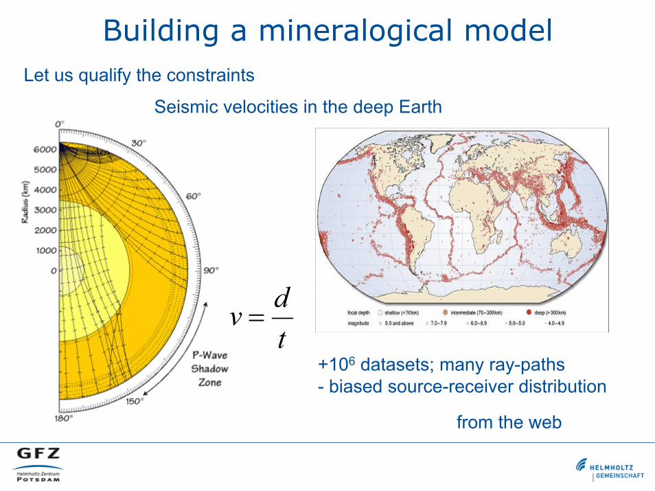
Building a mineralogical modelLet us qualify the constraints

from the web

Seismic velocities in the deep Earth

tdv =

+106 datasets; many ray-paths- biased source-receiver distribution


Deschamps and Tackley (2014)

density in the deep Earth

( ) ( ) ( ) ( )

SS

SSS

SSS

PK

TrrK

rrgdrd

PrP

r

⎟⎟⎠

⎞⎜⎜⎝

⎛∂∂

=

Δ+−

=⎟⎠⎞

⎜⎝⎛

⎟⎟⎠

⎞⎜⎜⎝

⎛∂∂

⎟⎠⎞

⎜⎝⎛∂∂

=⎟⎠⎞

⎜⎝⎛∂∂

ρρ

ραρρ

ρρ

,

,

2

Quasi-adiabatic self-compression(plus conductive boundary layers)


Deschamps and Tackley (2014)

Temperature in the deep Earth

( )( ) ( ) ( )

SS

PS

SSS

TrT

drdT

rrgCrTr

rT

rP

PT

rT

Δ+⎟⎠⎞

⎜⎝⎛∂∂

=

=⎟⎠⎞

⎜⎝⎛∂∂

⎟⎠⎞

⎜⎝⎛∂∂

⎟⎠⎞

⎜⎝⎛∂∂

=⎟⎠⎞

⎜⎝⎛∂∂

,

,

ρρα

Quasi-adiabatic temperature profile(conductive profiles for boundary layers)

Building a mineralogical modelLet us qualify the constraints The Earth cannot have a conductive temperature profile

ArTr

rrk

dtdT

+⎟⎠⎞

⎜⎝⎛

∂∂

∂∂

= 22

1

TC is unreasonably high for any reasonable set of parameters

22 , Ak

11, Ak

0=T

CT

Building a mineralogical model

MC ~ 0.01ME; VC ~ 0.02VE

P,T: Olivine - wadsleyite

P,T: ringwoodite – bridgmanite + ferropericlase

r: no vS

r: vs; P,T: melting of hcp-Fe

Relevant physical data

Heat flow

Building a mineralogical modelWe can neglect the crust (as a first approximation) The overall volume and mass of the crust are in the few percent level

MC ~ 0.01ME; VC ~ 0.02VE

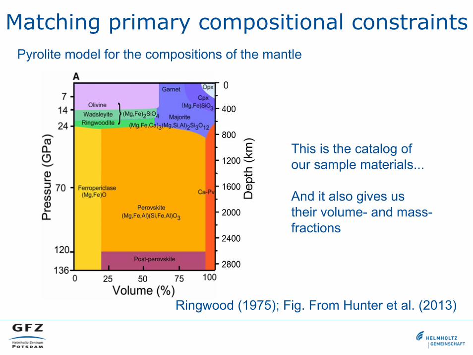
Matching primary compositional constraintsPyrolite model for the compositions of the mantle

Ringwood (1975); Fig. From Hunter et al. (2013)

This is the catalog of our sample materials...

And it also gives us their volume- and mass-fractions

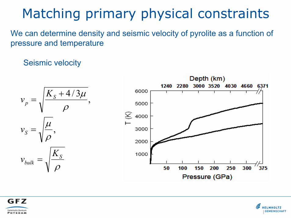
Matching primary physical constraintsWe can determine density and seismic velocity of pyrolite as a function of pressure and temperature

ρ

ρμ

ρμ

Sbulk

S

Sp

Kv

v

Kv

=

=

+=

,

,3/4

Seismic velocity

Matching primary physical constraintsDensity (and seismic velocity) of pyrolite as a function of P and T?

Large vol. press(LVP)

Diamond anvil cell(DAC)

Dynamic compres.(shock waves)

Using the diamond anvil cell (DAC)

Speziale (2003); T.S. Duffy webpage

Matching primary physical constraintsX-ray diffraction: It is clear that these experiments are still too challenging

Mostly for phase identification

Murakami et al. (2005); Ohta et al. (2008)

116 GPa, 1940K

110 GPa, 1960K

Matching primary physical constraintsMeasurements of single minerals to very high pressures and temperatures

Case of lower mantle phases

Mineral phase #Exp P(GPa) #HT #Vel(Mg,Fe,Al)(Si,Al,Fe)O3 bridgmanite 35 0 -180 ~10 7

(Mg,Fe,Al)(Si,Al,Fe)O3 postperovskite 23 0 -120 <10 5

(Mg,Fe)O ferropericlase 21 110 -200 ~5 0

CaSiO3 perovskite 6 0 -160 1 2

Mg3(Al,Fe,Mg,Si)2Si3O12 Garnet-majorite 16 0 - 26 10 12

Minor phases 3 0 -134 0 2

Matching primary physical constraintsX-ray diffraction data at high pressures and temperatures to refine the coefficients of the equation of state

Equation of state ρ(P,T)

ρ

ρμ

ρμ

Sbulk

S

Sp

Kv

v

Kv

=

=

+=

,

,3/4

Seismic velocity v(r,P,T)

KP=

∂∂ρρ

The equation of stateA successful model that describes volume (or density) data at very pressures is the Birch-Murnaghan EoS (B-M EoS)

( )

TT

T

TT

PKf

fPKffKP

⎟⎟⎠

⎞⎜⎜⎝

⎛∂∂

=⎥⎥⎦

⎤

⎢⎢⎣

⎡−⎟⎟

⎠

⎞⎜⎜⎝

⎛=

⎭⎬⎫

⎩⎨⎧

⎥⎦

⎤⎢⎣

⎡⎟⎠⎞

⎜⎝⎛∂∂

−−+=

ρρ

ρρ ,1

21

,4231213

3/2

0

0

2/50

Speziale et al. (2001)

MgO

Eulerian finite strain

( )

The same model is used to describe the pressure dependence of the elastic moduli from velocity measurements

( ) ,29142465321

,42

2753121

2

0000

00

000

2/5

2

00

2/50

⎭⎬⎫

⎩⎨⎧

⎥⎦

⎤⎢⎣

⎡⎟⎠⎞

⎜⎝⎛∂∂

+−−⎟⎠⎞

⎜⎝⎛∂∂

+⎥⎦

⎤⎢⎣

⎡−⎟

⎠⎞

⎜⎝⎛∂∂

−+=

⎭⎬⎫

⎩⎨⎧

⎥⎦

⎤⎢⎣

⎡−⎟

⎠⎞

⎜⎝⎛∂∂

+⎥⎦

⎤⎢⎣

⎡−⎟

⎠⎞

⎜⎝⎛∂∂

−+=

fPKKK

Pf

PKf

fPKf

PKfKK

S

SSSS

S

S

S

SSS

μμμμμμ

Murakami et al. (2008)

Fe-majorite

Isentropic EoSThe same form of the isothermal EoS can be used to calculate volumes along an isentropic compression path

( )

SS

S

SS

PKf

fPKffKP

⎟⎟⎠

⎞⎜⎜⎝

⎛∂∂

=⎥⎥⎦

⎤

⎢⎢⎣

⎡−⎟⎟

⎠

⎞⎜⎜⎝

⎛=

⎭⎬⎫

⎩⎨⎧

⎥⎦

⎤⎢⎣

⎡⎟⎠⎞

⎜⎝⎛∂∂

−−+=

ρρ

ρρ ,1

21

,4231213

3/2

0

0

2/50

Limitations of the approachIsentropic profiles of the different phases do not correspond to the same P-T path

from E.J. Garnero webpage

( )( ) ( ) ( )

( )( ) PS

PS

CrTr

PT

rrgCrTr

rT

ρα

ρρα

=⎟⎠⎞

⎜⎝⎛∂∂

=⎟⎠⎞

⎜⎝⎛∂∂ ,

Thermal EoSMie-Grüneisen approach to include the temperature effect

Uchida et al. (2001)

( ) ( ) ( ) ( )[ ]( ) ( ) ( )[ ],,,,

,,,,,

00

000

TVPTVPTVPVFP

TVFTVFTVFFTVF

ththcT

qqc

−+=⎟⎠⎞

⎜⎝⎛∂∂

−=

−++=

CP thPΔEq from Debye model (one free parameter, θ0)Overall 6 free parameters V0,KT0,(∂KT/∂P)T0,γ0, dlnγ/dlnVS, CV, α can be calculated



( ) ( ) ( ) ( )[ ]

P

S

V

T

V

qq

CVK

CVK

EPV

TVETVEV

TVPTVP

ααγ

γ

==⎟⎠⎞

⎜⎝⎛∂∂

=

−+= ,,,,, 000


( ) ( ) ,4231213,

0

2/500

⎭⎬⎫

⎩⎨⎧

⎥⎦

⎤⎢⎣

⎡⎟⎠⎞

⎜⎝⎛∂∂

−−+= fPKffKTVP

T

TT

DO

S

Debye approximation to determine E

Dω

ω

k Dk

ωε h=

λπω /2vkv ==333 /2/1/3 SP vvv +=

L/2π Dωω

( )3/2 LVq π=

( ) ( )3333 /2/4/2/4 LvLkN DD ππωππ ==

DD kv=ω

( ) 22 / vAddNDOS ω

ωω

==

( ) ( )ωεω DOSnE ∑= PVEH +=TSHG −=TSEF −=( ) ( )Tkn

B/exp11ω

ωh−

=

Sangster (Landolt – Börnstein Tables)

Comparison with the real phonon density of states

( ) ( )ωεω DOSnE ∑= PVEH +=TSHG −=TSEF −=( ) ( )Tkn

B/exp11ω

ωh−

=

DOS

Dωω



( ) ( ) ( ) ( )[ ]( ) ( ) ( )[ ]

( ) ( ) ( )[ ]

P

S

V

T

V

qq

ththcT

qqc

CVK

CVK

EPV

TVETVEV

EoSBMTVP

TVPTVPTVPVFP

TVFTVFTVFFTVF

ααγ

γ

==⎟⎠⎞

⎜⎝⎛∂∂

=

−+=

−+=⎟⎠⎞

⎜⎝⎛∂∂

−=

−++=

,,,,

,,,,

,,,,,

00

00

000


Summing minerals to make a rock(?)We can now calculate at each depth (i.e. P and T)

,,,,,, PS CKV αμρFrom prescribed mass fractions

for each mineral phase

∑=i

iXPyrolite

And we can calculate average (i.e. Pyrolite) properties

VPyroliteVXV

ParVX

ParasKParXParasCV

ii

ii

iiiiS

iiiP

/,1

,11,,,

==

=

∑

∑∑

ραα

μ

We can do the same for the inner core (IC ~ Fe) andSomething similar for the outer core (OC is liquid)

We can go a step furtherHaving the thermodynamic properties at each condition we can recalculate

(1) density as a function of radius

(3) moment of inertia I as a function of radius(I = Σi (mi di

2), d = distance from rotation axis)

( ) ( )( ) ( ) ( ) daaaMrMrKr

rrGM

r

R

rE

SS

22

2 4, ∫−=−=⎟⎠⎞

⎜⎝⎛∂∂ πρρρ

(2) temperature as a function of radius

( ) ( ) ( )( ) ( ) ( ) daaarMCrTr

rrGMr

rT drr

rPS

22 4, ∫

+

=−=⎟⎠⎞

⎜⎝⎛∂∂ πρ

ραρ

( )( ) ( ) ( ) ( )∫+

===drr

r

daaarMrrMrrrdrdI 2222 4,

324

32 πρπρ

We can go a step furtherHaving the thermodynamic properties at each condition we can recalculate

(1) density as a function of radius

(3) moment of inertia I as a function of radius(I = Σi (mi di

2), d = distance from rotation axis)

( ) ( )( ) ( ) ( ) daaaMrMrKr

rrGM

r

R

rE

SS

22

2 4, ∫−=−=⎟⎠⎞

⎜⎝⎛∂∂ πρρρ

(2) temperature as a function of radius

( ) ( ) ( )( ) ( ) ( ) daaarMCrTr

rrGMr

rT drr

rPS

22 4, ∫

+

=−=⎟⎠⎞

⎜⎝⎛∂∂ πρ

ραρ

( )( ) ( ) ( ) ( )∫+

===drr

r

daaarMrrMrrrdrdI 2222 4,

324

32 πρπρ

Main limitations – Can we do better? Our minerals have fixed compositions

The mineral proportions are now energetically inconsistent with our set of thermodynamic data for the single phases

We need a thermodynamic model to determine self-consistently equilibrium assemblages (min. free energy) and all the elastic properties of the phases

One example (which I like because it includes anisotropic properties):Stixrude and Lithgow-Bertelloni [Geoph. J. Inter., (2005),162, 610; Geoph. J. Inter., (2011),184, 1180

Key concept: G(P,T) = F(V,T) + P(V,T)V

How can we do better?Improving the thermodynamic databaseMore phase stability data

Litasov and Ohtani (2007)

How can we do better?Improving the thermodynamic databaseMore phase stability data

Dorfman et al. (2014)

pPv postperovskitePv bridgmaniteMw ferropericlaseSt stishovite (SiO2)Mj majorite

How can we do better?More Equation of state data V(P,T,X)

Bridgmanite (Mg,Fe)SiO3

Dorfman et al. (2014)

How can we do better?More Elasticity data v(P,T,X), KS(P,T,X), μ(P,T,X)

Murakami et al. (2012)

Al-MgSiO3 and MgSiO3

(Mg,Fe)O and MgO

The Earth is not radially symmetricSeismology shows large lateral heterogeneity and the presence anisotropy at all depths

Masters et al. (2000); Lay and Garnero (2011)

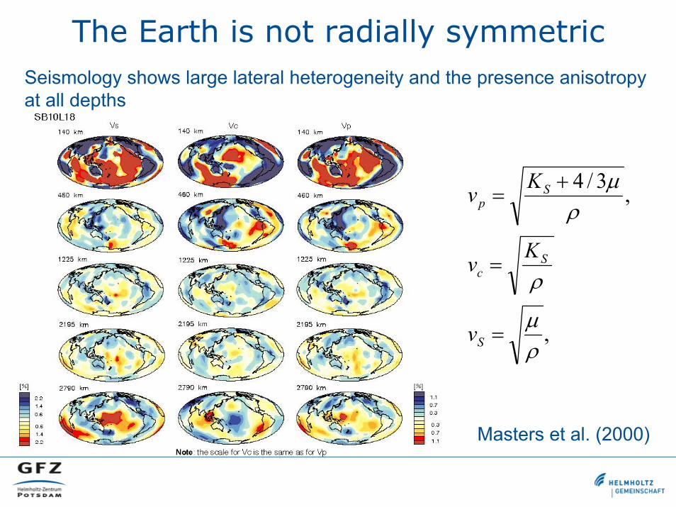
The Earth is not radially symmetricSeismology shows large lateral heterogeneity and the presence anisotropy at all depths

Masters et al. (2000)

,

,3/4

ρμ

ρ

ρμ

=

=

+=

S

Sc

Sp

v

Kv

Kv

The Earth is isotropicSeismology shows large lateral heterogeneity and the presence anisotropy at all depths

Evidences of shear wave anisotropy in D’’ (2700-2900 km depth)

Nowacki et al. (2011)

The Earth is isotropicSeismology shows large lateral heterogeneity and the presence anisotropy at all depths



21

212SS

SSS vv

vvv+−

=δ

The Earth is not isotropicSeismology shows large lateral heterogeneity and the presence anisotropy at all depths



Wookey et al. (2008)

For anisotropic Earth modelsMore studies of the physical anisotropy of minerals at high P and T

MgSiO3(Mg,Fe)SiO3(Mg,Fe)(Al,Si)O3

Bridgmanite

Boffa Ballaran et al. (2012); Lu et al. (2013)

(Mg,Fe)3Al2Si3O12

We need effective approaches to model rocks anisotropy

For anisotropic Earth models

1.4

1.2

1.0

0.8

0.6

0.4

0.2

0.0

A=

2C44

/(C11

- C

12)

706050403020100

Pressure (GPa)

Brillouin Radial diffraction Theoretical (Karki and Crain, 1998)

z

x y

z

x y

z

x yX

X

X Y

Z

Y

Z

Y

Z

Young’s modulus

1 bar

25.2 GPa

65.2 GPa

CaO Pakistani Himalaya

The Earth is dynamicHeterogeneity and anisotropy in the Earth are connected to its internal dynamics

from H.B. Bunge webpage; Nowacki et al. (2011)

Experimental study of texturing at high pressures and temperatures


f(g)dg = dVg/V

Texture and elastic anisotropy computations for prescribed strain fields

Wenk et al. (2006)

Geodynamic simulation

Computed strain

Computed elastic anisotropy

(experiments + simulation)


( )dggfCggggC pqrslskrjqipijkl'∫∫∫=

ReferencesFowler (2005), The Solid Earth: An Introduction to Global Geophysics, Cambridge Univ. Press

Cole and Woolfson (2002), Planetary Science: The Science of Planets Around Stars, Institute of Physics

Poirier (2000) , Introduction to the Physics of the Earth Interiors, Cambridge Univ. Press

Stixrude and Lithgow-Bertelloni (2005), Thermodynamic of mantle minerals – I. Physical properties

Stixrude and Lithgow-Bertelloni (2005), Thermodynamics of mantle minerals – II. Phase equilibria

Documents

Elastic and thermal properties of the Earth interior · Elastic and thermal properties of the Earth interior S. Speziale German Research Centre for Geosciences GFZ . Our static picture