Embed Size (px)
Citation preview
HAL Id: tel-02001195https://tel.archives-ouvertes.fr/tel-02001195
Submitted on 31 Jan 2019
HAL is a multi-disciplinary open accessarchive for the deposit and dissemination of sci-entific research documents, whether they are pub-lished or not. The documents may come fromteaching and research institutions in France orabroad, or from public or private research centers.
L’archive ouverte pluridisciplinaire HAL, estdestinée au dépôt et à la diffusion de documentsscientifiques de niveau recherche, publiés ou non,émanant des établissements d’enseignement et derecherche français ou étrangers, des laboratoirespublics ou privés.
Elastic matching for classification and modelisation ofincomplete time series
Thi-Thu-Hong Phan
To cite this version:Thi-Thu-Hong Phan. Elastic matching for classification and modelisation of incomplete time se-ries. Signal and Image processing. Université du Littoral Côte d’Opale, 2018. English. �NNT :2018DUNK0483�. �tel-02001195�
Numéro d’ordre:École doctorale SPI - Université Lille Nord-De-France
THESISSubmitted for the degree of
Doctor of Philosophy (PhD) in Signal Processing
Docteur de l’Université Littoral Côte d’OpaleDiscipline: Traitement du signal
Thi-Thu-Hong PHANCalais, October 2018
Elastic matching for classification andmodelisation of incomplete time series
sous la direction de / Thesis supervisors:
André BIGAND Maître de Conférences - HDRÉmilie POISSON CAILLAULT Maître de Conférences
JURY - Thesis committee:
Plamen ANGELOV Professeur, Lancaster University Rapporteur / RefereeChristian VIARD GAUDIN Professeur, Université de Nantes Rapporteur / RefereeSylvie Le HÉGARAT-MASCLE Professeur, Université Paris Sud Présidente / PresidentAlain LEFEBVRE Chercheur expert HDR Invité / Invited member
Dir. IFREMER LER Boulogne-sur-mer
Laboratoire d’Informatique, Signal et Image de la Côte d’Opale – EA 449150 rue Ferdinand Buisson – B.P. 719, 62228 Calais Cedex, France

Contents
Notations and Abbreviations iii
Introduction 5
1 Preliminaries 111.1 Time series . . . . . . . . . . . . . . . . . . . . . . . . . . . . . . . . . . . . 12
1.2 Missing data mechanisms . . . . . . . . . . . . . . . . . . . . . . . . . . . . . 12
1.3 Time series characterization . . . . . . . . . . . . . . . . . . . . . . . . . . . 15
1.3.1 Composition of time series . . . . . . . . . . . . . . . . . . . . . . . . 15
1.3.2 Auto-correlation function (ACF) . . . . . . . . . . . . . . . . . . . . . 16
1.3.3 Correlation . . . . . . . . . . . . . . . . . . . . . . . . . . . . . . . . 18
1.3.4 Cross-correlation (recurrent data for univariate time series) . . . . . . . 18
1.4 Experiments protocol . . . . . . . . . . . . . . . . . . . . . . . . . . . . . . . 19
1.4.1 Experimental process for the imputation task . . . . . . . . . . . . . . 20
1.4.2 Measurements for evaluating imputation methods . . . . . . . . . . . . 20
1.5 Chapter conclusion . . . . . . . . . . . . . . . . . . . . . . . . . . . . . . . . 24
2 DTW-based imputation approach for univariate time series 252.1 Introduction . . . . . . . . . . . . . . . . . . . . . . . . . . . . . . . . . . . . 26
2.2 Literature review of Dynamic Time Warping . . . . . . . . . . . . . . . . . . . 28
2.2.1 Classical DTW algorithm . . . . . . . . . . . . . . . . . . . . . . . . 28
2.2.2 DDTW - Derivative Dynamic Time Warping . . . . . . . . . . . . . . 32
2.2.3 AFBTW - Adaptive Feature Based Dynamic Time Warping . . . . . . 33
2.2.4 Dissimilarity-based elastic matching . . . . . . . . . . . . . . . . . . . 34
2.2.5 Dynamic Time Warping-D algorithm (DTW-D) . . . . . . . . . . . . 35
2.2.6 Illustration . . . . . . . . . . . . . . . . . . . . . . . . . . . . . . . . 35
2.3 Dynamic Time Warping-based imputation for univariate time series . . . . . . 41
2.3.1 The proposed method - DTWBI . . . . . . . . . . . . . . . . . . . . . 41
2.3.2 Validation procedure . . . . . . . . . . . . . . . . . . . . . . . . . . . 44
2.3.3 Results and discussion . . . . . . . . . . . . . . . . . . . . . . . . . . 47
2.3.4 Conclusion . . . . . . . . . . . . . . . . . . . . . . . . . . . . . . . . 57
2.4 Comparison of various DTW versions for completing missing values in uni-
variate time series . . . . . . . . . . . . . . . . . . . . . . . . . . . . . . . . . 58
2.4.1 Introduction . . . . . . . . . . . . . . . . . . . . . . . . . . . . . . . . 58
2.4.2 Imputation based on DTW metrics . . . . . . . . . . . . . . . . . . . . 59
2.4.3 Data presentation . . . . . . . . . . . . . . . . . . . . . . . . . . . . . 59
2.4.4 Results and discussion . . . . . . . . . . . . . . . . . . . . . . . . . . 60
2.4.5 Conclusion . . . . . . . . . . . . . . . . . . . . . . . . . . . . . . . . 64
2.5 Chapter conclusion . . . . . . . . . . . . . . . . . . . . . . . . . . . . . . . . 66
3 Imputation approaches for uncorrelated multivariate time series 693.1 Introduction . . . . . . . . . . . . . . . . . . . . . . . . . . . . . . . . . . . . 69
3.2 Dynamic Time Warping-based uncorrelated multivariate time series imputation 73
3.2.1 DTWUMI - Proposed approach . . . . . . . . . . . . . . . . . . . . . 73
3.2.2 Validation procedure . . . . . . . . . . . . . . . . . . . . . . . . . . . 75
3.2.3 Results and discussion . . . . . . . . . . . . . . . . . . . . . . . . . . 79
3.2.4 Conclusion . . . . . . . . . . . . . . . . . . . . . . . . . . . . . . . . 84
3.3 Proposed method based on an hybrid similarity measure . . . . . . . . . . . . 85
3.3.1 Methods based on fuzzy similarity measure . . . . . . . . . . . . . . . 85
3.3.2 FSMUMI-Proposed approach . . . . . . . . . . . . . . . . . . . . . . 87
3.3.3 Validation procedure . . . . . . . . . . . . . . . . . . . . . . . . . . . 93
3.3.4 Results and discussion . . . . . . . . . . . . . . . . . . . . . . . . . . 96
3.3.5 Conclusion . . . . . . . . . . . . . . . . . . . . . . . . . . . . . . . . 107
3.4 Chapter conclusion . . . . . . . . . . . . . . . . . . . . . . . . . . . . . . . . 107
4 Applications: Toward classification and forecasting 1114.1 Classification of phytoplankton species . . . . . . . . . . . . . . . . . . . . . 112
4.1.1 Introduction . . . . . . . . . . . . . . . . . . . . . . . . . . . . . . . . 112
4.1.2 Feature-extraction algorithm . . . . . . . . . . . . . . . . . . . . . . . 115
4.1.3 Methodology . . . . . . . . . . . . . . . . . . . . . . . . . . . . . . . 116
4.1.4 Experiment and discussion . . . . . . . . . . . . . . . . . . . . . . . . 121
4.1.5 Conclusion . . . . . . . . . . . . . . . . . . . . . . . . . . . . . . . . 125
4.2 Event detection in a multidimensional time series . . . . . . . . . . . . . . . . 125
4.2.1 Data presentation . . . . . . . . . . . . . . . . . . . . . . . . . . . . . 126
4.2.2 Preprocessing data . . . . . . . . . . . . . . . . . . . . . . . . . . . . 129
4.2.3 Event detection . . . . . . . . . . . . . . . . . . . . . . . . . . . . . . 132
4.2.4 Conclusion . . . . . . . . . . . . . . . . . . . . . . . . . . . . . . . . 134
4.3 Comparative Study on Univariate Forecasting Methods for Meteorological Time
Series . . . . . . . . . . . . . . . . . . . . . . . . . . . . . . . . . . . . . . . 136
4.3.1 Introduction . . . . . . . . . . . . . . . . . . . . . . . . . . . . . . . . 136
4.3.2 Time series forecasting methods . . . . . . . . . . . . . . . . . . . . . 138
4.3.3 Experiment protocol . . . . . . . . . . . . . . . . . . . . . . . . . . . 140
4.3.4 Results and discussion . . . . . . . . . . . . . . . . . . . . . . . . . . 141
4.3.5 Conclusion . . . . . . . . . . . . . . . . . . . . . . . . . . . . . . . . 145
4.4 Chapter conclusion . . . . . . . . . . . . . . . . . . . . . . . . . . . . . . . . 146
Conclusions and future work 149
Appendices 155
A List of publications and valuations related to the thesis 157
B Illustration of different DTW versions matching 161
C List of fuzzy rules 165
D Dynamic Time Warping-based imputation for univariate time series data 169
Bibliography 179
List of Tables 197
List of Figures 199
Abstract 203


Acknowledgment
Firstly, I would like to take this opportunity to express my deepest appreciation and thank to
my supervisors Professor André BIGAND, Associate Professor Emilie POISSON CAILAUT
for your support and guidance; you have been tremendous mentors for me. Your meticulous
comments were of enormous assistance to me, and without your guidance and persistent help
this thesis would not have been possible.
I would like to express my special gratitude to Prof. Plamen ANGELOV and Prof. Christian
VIARD GAUDIN for their time and hard work to review my thesis, and for giving me valuable
remarks to improve it. I would also like to convey special thanks to Prof. Sylvie Le HÉGARAT-
MASCLE and Dr. Alain LEFEBVRE for examining my dissertation.
I am grateful to Wagner Anne, Sandrine Target for their patience and advice to help me
improve the quality of my writing. I am also indebted to the members of the IFREMER
institute (France), Nguyen Duy Binh (VNUA-Vietnam) for the databases and SCoSI/ULCO
(CALCULCO computing platform) for experiments.
Next, I would like to thank the Vietnam International Education Development, Campus
France and LISIC laboratory - University of Littoral for funding this thesis. Without their
financial support this project could not have happened.
I also would like to acknowledge my colleagues at the Computer Science Department of
Vietnam National University of Agriculture for their moral support throughout the whole PhD.
I am grateful to Pham Quang Dung and Farouk Yahaya for kindly volunteering to proofread
chapters.
I also would like to thank all my lab colleagues at LISIC and friends for their interaction
and friendly support during these years. I am greatly indebted to LE Hoang Raymond, Danielle
Proust who have constantly motivated me throughout this work. There are so many people I
am thankful for, and while I cannot thank each one individually, I am blessed to have had so
much support along the way.

Most importantly, I am incredibly grateful to my husband for his love, patience and en-
couragement during these challenging academic years. I am thankful for my children who
always brighten my days and keep life in perspective. I convey special thanks to my parent, my
brothers, and sisters. Their love, support and belief were what sustained me thus far.

Notations and Abbreviations
Notationst Position of the first missing value of a gapT Size of a gapM Number of columns/ Number of variablesN Number of instantsx Univariate time seriesX Multivariate time seriesQ QueryR ReferenceQs The most similar windowQa Query after the gapQb Query before the gapQas The most similar window after the gapQbs The most similar window before the gap
AbbreviationsAFBDTW Adapted Feature Based Dynamic Time WarpingANN Artificial Neural NetworksARIMA Autoregressive Integrated Moving AverageBSTS Bayesian Structural Time SeriesDDTW Derivative Dynamic Time WarpingDT Decision TreeDTW Dynamic Time WarpingDTWBI Dynamic Time Warping-based ImputationDTWUMI Dynamic Time Warping-based Uncorrelated Multivariate ImputationED Euclidean DistanceES Exponential SmoothingFB Fractional Bias
iii
FcM Fuzzy c-MeanFCM Flow CytoMetryFFNN Feed-Forward Neural NetworkFSD Fraction of Standard DerivationFSMUMI Fuzzy Similarity Measure-based Uncorrelated Multivariate ImputationFLO Orange FluorescenceFLR Red FluorescenceFLY Yellow FluorescenceFWS Forward Scatterk-NN k-Nearest NeighborsLDA Linear Disciminant AnalysisLMCF Last Mean Carried ForwardLOCF Last Observation Carried ForwardLR Linear RegressionMAR Missing At RandomMCAR Missing Completely At RandomMNAR Missing Not At RandomMI Multiple imputationMICE Multiple Imputation by Chained EquationsML Maximum LikelihoodMLP Multi-Layer PerceptronNA Not AvailableNB Naive BayesNMAE Normalized Mean Absolute ErrorPCA Principal Component AnalysisRBF Radial Basis FunctionRF Random ForestRRF Regularized Random ForestGRRF Guided Regularized Random ForestGRF Guided Random ForestRMSE Root Mean Standard ErrorSARIMA Seasonal-ARIMASD Standard DeviationSE Standard ErrorSES Single Exponential SmoothingSnaive Seasonal naiveSVM Support Vector MachineSWS Sideward Scatter
Introduction
Context of the subject
Huge time series can now be considered thanks to the availability of effective low-cost sensors,and the wide deployment of remote sensing systems. But collected data are commonly incom-plete for various reasons such as sensor errors, transmission problems, incorrect measurements,bad weather conditions (outdoor sensors) for manual maintenance, etc. Missing data are a ma-jor drawback which particularly affects marine samples [1, 2]. An example of recent data is acharacterization of seawater collected by the MAREL Carnot station. This station is a marinewater monitoring platform in the eastern English Channel located in Boulogne-sur-Mer, France([3]). Its objective is to find out how the bloom of algae (phytoplankton) disrupted the coastalecosystem of the eastern Channel. The aforementioned data contain 19 large time series sam-pled every 20 minutes including fluorescence, turbidity, oxygen saturation, . . . , and measuredby sensors. The analysis of this dataset with extraordinary size and shape allows us to revealevents such as algal blooms and to understand phytoplankton processes in detail. But the datainclude a vast number of missing values viz., 62.2% for phosphate, 59.9% for nitrate, 27.22%for pH, 12.32% for fluorescence and so on.
Most of proposed models for time series analysis suffer from one major drawback, which istheir inability to process incomplete datasets, despite their powerful techniques. They usuallyrequire complete data, ie. without missing values (MV). Missing data produce a loss of infor-mation and can generate inaccurate data interpretation. So how can missing values be dealtwith? Ignoring or deleting is a simple way to solve this drawback (also known as completecase analysis). However, this solution has to pay a high price because of losing valuable in-formation, especially when dealing with a small dataset. This is prominent in time series datawhere the considered values depend on the previous ones. Furthermore, an analysis based onthe systematic differences between observed and unobserved data leads to biased and unreli-able results [4]. Thus, the filling procedure is a mandatory and precursory pre-processing stepbefore performing other steps such as modeling/classification, etc. The imputation techniqueis a conventional method to handle the MV problem [5]. In addition, it is necessary to select orpropose imputation methods that suit to the type of data and that are consistent with the missing
5
values mechanism.
For low frequency systems with a monthly sampling or small missing sequence, they canbe easily filled in and they do not affect the global results. In this case, a linear or polynomialregression (of order 2) can use to complete missing values. But problems arise when completingmissing values of high frequency systems with quick dynamics change such as MAREL Carnotdata and purpose [6]. Moreover, the lack of data is not randomly distributed and the size ofconsecutive missing values (called a gap) is large. The analysis of such data can result inbiased interpretations. For example, pH signal contains the largest gap of 234 days, and in thiscase, we cannot detect phytoplankton bloom (this can only occur in a duration of one day toone month). Thus, imputation techniques such as moving average or regression methods arenot effective. Completion becomes more complex when adding variability (and noise) due tothe high frequency system.
In other words, for time series data, present values and past ones are often related. Thus, it isimportant to consider the whole history (i.e. dynamics) of each signal to complete each gap. Todeal with the problem of missing values, a natural solution is to look for the same behavior orshape within time series which amounts to retrieving similar values in the series before or afterthe missing values. Then missing data are completed with the sequence of following/previoussimilar values.
Approaches and methodology
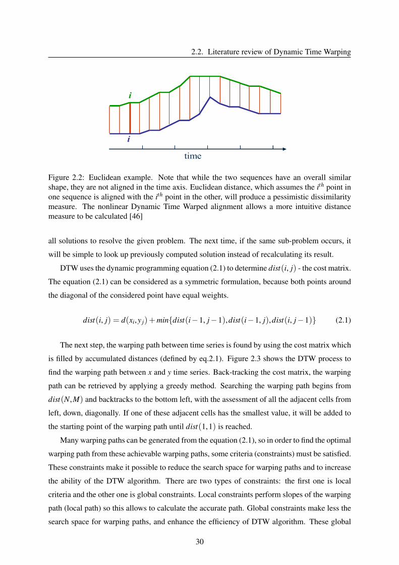
Dynamic Time Warping (DTW, also called elastic matching) [7] is an effective and well-knownmethod for measuring similarity between two linear/nonlinear time series. The success of DTWin data mining [8], information retrieval and pattern recognition [9, 10, 11] leads us to studyits ability to complete missing values in our context of detection and modelization of eventstates from time series data. This method calculates a geometric distance between two curvesto assess their similarity. The method accepts temporal and local expansions. The algorithmconsists in mapping pairs of points that minimizes the Euclidean distance between them, so anoverall similarity cost is defined as a sum of intensity distance between all paired points.
The elastic matching is widely used in speech or handwriting recognition. Sakoe and Chiba[7] proposed this method to calculate the elastic distance in recognizing spoken words (a wordcan be pronounced with different sound and length variation). For handwriting recognition,Rath and Manmatha [12] used images of words in their experience and showed that the elasticpairing was an effective method to take into account a spatial variability of the word. DTWmatching cost was also used for data classification [13]. Petitjean et al. [14] proposed the DBA(DTW Barycenter Averaging) approach to compute an average of a set of sequences underDTW. Then, DBA was particularly used instead of the Euclidean distance in the K-meansalgorithm to successfully cluster satellite image time series.
6
Another class of approaches to handle missing data problem is the fuzzy set theory. Thistheory makes it possible to deal with imprecise and uncertain circumstances [15]. Imprecisionis classically due to sensors. Hence, time series can be considered as fuzzy as pointed out byChen et al. [16]. Unfortunately, time series are also saddled by problems of incompleteness(missing data) and randomness (noise). This inclines us to focus on fuzzy similarity measuresby proposing a more generic uncertainty model. Our study follows the success of existingtechniques of weighting similarity measures and fuzzy-based similarity measure. Indeed, thesemethods tend to produce accurate predictions. Some notable areas where weighted similar-ity measures are employed are numerous as retrieval systems [15], recommendation systems[17], and collaborative filtering [18, 19]. While fuzzy-based similarity measure has also beensuccessfully used in [20, 15, 17] .
The robustness of these approaches has opened a new scope by weighting similarity mea-sures based on fuzzy logic to solve the incompleteness problem in time series data. A classicalapproach to build a new fuzzy-weighted similarity measure is to use a rule-based technique.This technique has been widely implemented in different applications like online learning [21],time series prediction [22], knowledge extraction from data streams [23], equilibrium problemin economics [24] or in [15], and so on. These potentials lead us to deploy a rule-based tech-nique to build a fuzzy-weighted similarity measure which is applied to complete large missingvalues in uncorrelated multivariate time series.
Contributions of the PhD thesis
The thesis focuses on the investigation and the development of algorithms to complete missingvalues in time series. Two types of data are studied to propose imputation methods includingunivariate and uncorrelated multivariate time series. The contributions of the study are statedas follows:
• The first contribution is the proposition of new features allowing better describe globalshape and dynamics of a signal (named, shape-feature extraction algorithm). This al-gorithm is then used to extract features of phytoplankton signals in order to identifyphytoplankton species.
• Our second contribution is to propose an effective method, namely DTWBI (DTW BasedImputation), to complete successive missing data in mono-dimensional time series. Thismethod is based on the combination of the proposed shape-feature extraction and Dy-namic Time Warping approaches. The performance of the algorithm is compared withpublished methods on various real and synthetic databases. We then propose a frameworkto compare the performance of different DTW variants for the univariate imputation taskin marine context.
• The third contribution is an extension of DTWBI to fill large missing data in low/un-correlated multivariate time series, called DTWUMI (DTW based Uncorrelated Mul-
7
tivariate Imputation). This approach is also based on the elastic matching and shape-feature extraction algorithms. A comparison between DTWUMI approach and state-of-the-art algorithms is implemented to assess the performance of the proposed algorithmon different real and simulated databases.
• The fourth contribution focuses on developing a novel approach for filling successivemissing values in low/un-correlated multivariate time series with a high level of uncer-tainty management, namely FSMUMI (Fuzzy Similarity Measure based UncorrelatedMultivariate Imputation). In this way, we propose to use a novel fuzzy weighted simi-larity measure based on fuzzy grades of basic similarity measures and fuzzy rules. Toevaluate the ability of the proposed approach, we compare it with other published meth-ods on various large time series.
• The final contributions are concrete applications of the DTWBI method i) to complete theMAREL Carnot database and then perform a detection and characterization of usual/rareevents in these time series and ii) to forecast univariate meteorological time series col-lected in Vietnam.
Outline of the PhD thesis
The manuscript is divided into three parts: an introductory part presenting general notionsand mechanisms related to missing data, the experiment protocol and indicators to evaluateimputation methods (Chapter 1), a main part covering the completion of the missing data inmono-dimensional and multidimensional time series (Chapters 2 and 3), then an applicationpart dedicated to classify phytoplankton species, detect rare/extreme events in a real datasetand forecast univariate meteorological time series (Chapter 4).
Chapter 1 first introduces the definition of univariate/multivariate time series. It then presentsthe mechanism of missing data described by Little and Rubin ([25]) and our concepts about cat-egorization of missing values. The characterization of univariate time series is also discussed.Finally, the design of the experiments is mentioned including the experimental protocol for theimputation task and criteria using to evaluate completion algorithms.
Chapter 2 is devoted to the first main contribution of this thesis. It provides the basicfoundation of Dynamic Time Warping approach and how the DTW works. A review of differentversions of DTW is also presented. A new imputation approach (DTWBI) for univariate timeseries is proposed. This approach is based on the combination of the shape-feature extractionand Dynamic Time Warping methods. Another contribution of this chapter is the proposition ofa framework for filling missing values in univariate time series. Thus a comparison of differentversions of DTW is performed for the imputation task. The goal is to identify the most suitablemethods for the imputation of marine univariate time series ensuring that results are reliableand high quality.
8
Chapter 3 highlights the second main contribution of this study. We propose two novelmethods to estimate missing data for low/un-correlated multivariate time series. In these twoapproaches, we take advantage of the property of low/un-correlated multivariate data but weexploit this feature in two different aspects. In the first approach, we apply the major principleof DTW method and shape-feature extraction algorithm to complete large missing values. Inthe second approach, we impute large gaps in low/un-correlated multivariate data with a highlevel of uncertainty. In this way, we build a new hybrid similarity measure based on fuzzygrades of basic similarity measures and on fuzzy logic rules. Experimental results of the twoproposed approaches are compared with results obtained from the state-of-the-art methods.
Chapter 4 corresponds to applications of the shape-feature extraction algorithm and DTWBIapproach via three specific developments:
• The first application focuses on the classification of phytoplankton species. Accordingly,we propose the shape-feature extraction algorithm to extract features of phytoplanktonsignals obtained from flow cytometry (FCM). We then compare the performance of vari-ous classifiers on the proposed type of features and two other types of features to find themost convenient features type for the classification of phytoplankton.
• The second part of this chapter is devoted to high frequency MAREL Carnot data. Theobjective is to complete missing values of this dataset and then carry out a detection ofrare/extreme events using multi-level spectral clustering approach.
• The third part is dedicated to compare univariate forecasting methods for meteorologicaltime series. Inspired from the imputation process, we apply DTWBI to forecast univariatetime series and perform a comparison of different univariate forecasting algorithms.
Finally, we conclude this PhD thesis with a highlight of our contributions and discuss pos-sibilities for further research that could be investigated.
This thesis is a part of CPER MARCO project (marco.univ-littoral.fr) and is made in collab-oration with IFREMER LER-BL (https://wwz.ifremer.fr/manchemerdunord/Environnement/LER-Boulogne-sur-Mer), LOG UMR CNRS (http://log.cnrs.fr) and VNUA (http://www.vnua.edu.vn/).
9

10
Chapter 1Preliminaries
Contents1.1 Time series . . . . . . . . . . . . . . . . . . . . . . . . . . . . . . . . . . . 12
1.2 Missing data mechanisms . . . . . . . . . . . . . . . . . . . . . . . . . . . 12
1.3 Time series characterization . . . . . . . . . . . . . . . . . . . . . . . . . 15
1.3.1 Composition of time series . . . . . . . . . . . . . . . . . . . . . . . 15
1.3.2 Auto-correlation function (ACF) . . . . . . . . . . . . . . . . . . . . 16
1.3.3 Correlation . . . . . . . . . . . . . . . . . . . . . . . . . . . . . . . 18
1.3.4 Cross-correlation (recurrent data for univariate time series) . . . . . . 18
1.4 Experiments protocol . . . . . . . . . . . . . . . . . . . . . . . . . . . . . 19
1.4.1 Experimental process for the imputation task . . . . . . . . . . . . . 20
1.4.2 Measurements for evaluating imputation methods . . . . . . . . . . . 20
1.5 Chapter conclusion . . . . . . . . . . . . . . . . . . . . . . . . . . . . . . 24
This chapter introduces some background concepts related to time series and also inves-
tigates the design of experiments. Section 1.1 discusses what are time series. Missing data
definition and missing data mechanisms are then provided in Section 1.2. Section 1.3 mentions
the characterization of univariate time series. Finally, Section 1.4 presents the experiments pro-
tocol for the imputation task (this technique is applied to mono-dimensional and multidimen-
sional imputation methods) including experimental process and performance measurements of
imputation algorithms.
11
1.1. Time series
1.1 Time series
A time series is a collection of observations (a sequence of data points), typically consisting of
successive measurements made over a time interval.
Lots of useful information can be obtained from collected time series. They are very com-
mon in statistics, signal processing, pattern recognition, econometrics, mathematical finance,
weather forecasting, intelligent transport and trajectory forecasting, earthquake prediction, con-
trol engineering, astronomy, communications engineering, and largely in any domain of applied
science and engineering which involves temporal measurements.
Usually, we can distinguish univariate from multivariate time series. We use capital letters
to denote multi-variables, and lowercase letters to denote univariate.
Univariate time series refers to data from one variable recorded sequentially in uniform
intervals, for example, hourly energy consumption, daily temperature in a city. x = {xt |t =1,2, · · · ,N} denotes a univariate time series of N successive observations indexed in time.
Multivariate time series is used when a group of time series variables are involved and their
interactions may be considered. A multivariate time series is represented as a matrix XN×M
with M collected signals of length N. x(t, i) denotes the value of the i-th signal at time t.
xt = {x(t, i), i = 1, · · · ,M} is the vector at the t-th observation of all variables.
1.2 Missing data mechanisms
Missing data, or missing values infer the existence of observations whose values are either not
collected or lost after registering or corresponding to wrong values (out of the sensor range) in
the database. In the literature, missing data mechanisms can be divided into three categories.
Each category is based on one possible cause: "Missing data are completely random" (Missing
Completely At Random, MCAR, in the literature), "Missing data are random" (Missing At
Random, MAR) and "Missing data are not random" (Missing Not At Random, MNAR) ([25]).
A detailed discussion is presented as follows:
• Missing Completely At Random, MCAR
Missing data are considered as MCAR when the missingness of data is unrelated to any
value (the values of missing variable itself or the values of any other variable). This
means these missing data points make a random subset of the data and are completely
unsystematic. For example, when a person refuses to disclose his income, this does not
12
CHAPTER 1. PRELIMINARIES
affect his actual income nor the income of his family. Similarly, ignoring MCAR missing
values does not make the data analysis biased but will increase the standard error of the
sample estimates due to the reduced sample size [26].
• Missing At Random, MAR
Missing data are MAR, that means probability of missing values depends only on the
observed data, but not the missing data. In the other hand, the missing values of a variable
depend on available values of itself and other variables. This makes it possible to estimate
missing data based on other variables. For instance, evaluating students participating in a
subject includes two exams: midterm exam and final one. In order to take the final exam
students must pass the midterm exam. Assuming that a student fail the midterm exam
and he/she drops out of the course. Thus, the missing final exam for this student is MAR.
• Missing Not At Random, MNAR
Missing data are MNAR if the propensity of missing values depends on other missing
values. Thus with this type of missing data, we cannot estimate incomplete data from
existing variables. To extend the previous example, when a student may pass the midterm
exam but he/she may be absent at for the final exam.
It is important to understand causes that produce missing data in order to develop an adapt-
able imputation task. This can in-turn aid in the selection or proposition of an appropriate
imputation algorithm ([27]). But in practice, understanding the causes remains a challenging
task when missing data cannot be known at all, or when these data have a complex distribution
([28]).
We note that these missing mechanisms are just assumptions about reasons for the lack of
data in the context of analysis. Thus from a hypothetical standpoint, they cannot be verified
(except for the MCAR hypothesis) and there are no characteristics of the data itself. Similarly,
assigning sub-sequences of missing values to "a category can be blurry" ([27]). Commonly,
most current research works focus on the three types of missing data previously defined to find
out corresponding imputation methods. But Molenberghs et al. advised that it would always be
better to check the robustness of the analytical results to different assumptions with sensitivity
analysis ([29], Part V). For these reasons, in this study, we consider missing data as 2 types:
isolated missing values and gap - missing consecutive values. Let consider some terminologies
and a real marine dataset to illustrate the problem.
13
1.2. Missing data mechanisms
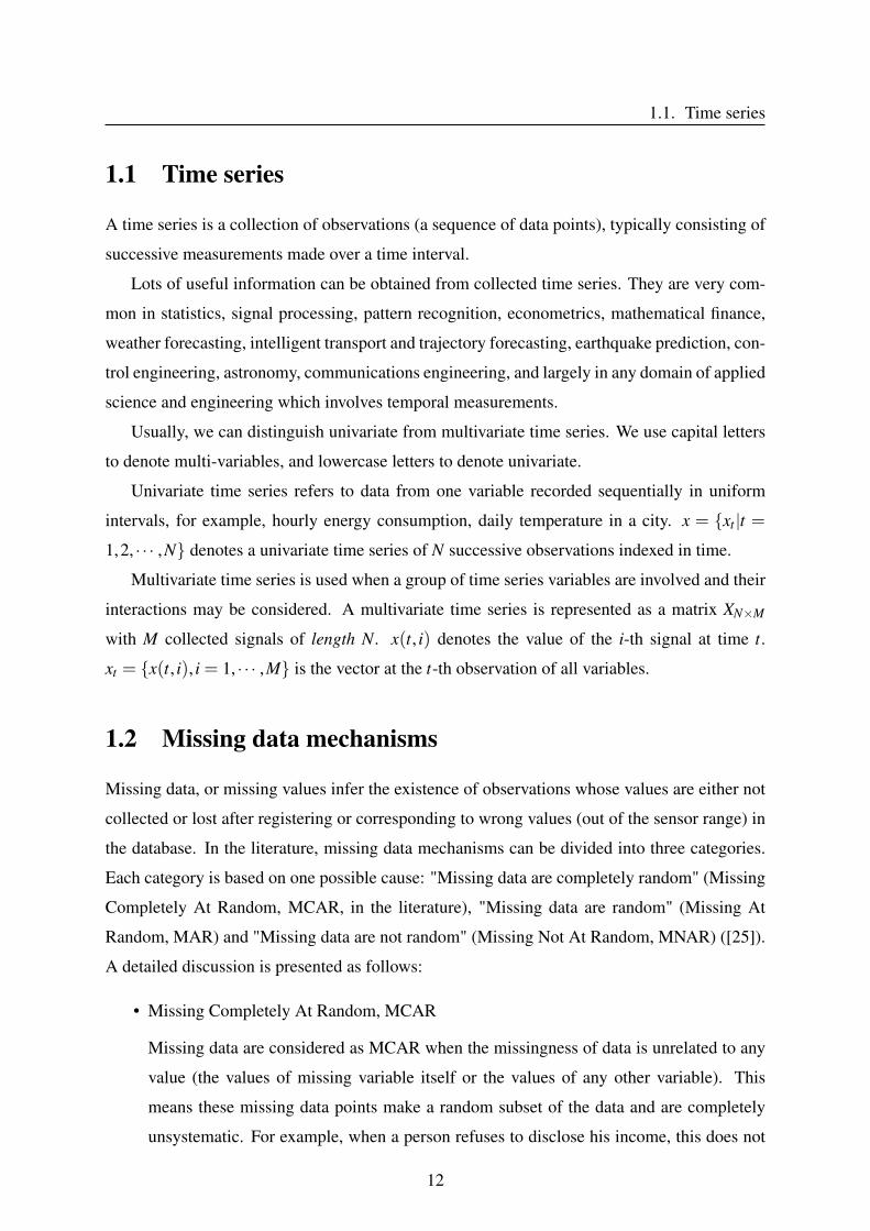
Figure 1.1: Illustration of isolated and T-gap missing values
• Isolated missing value
Given an univariate time series x = {xt |t = 1,2, · · · ,N} with N observations. A single
hole at time t is an isolated missing value when observations at time t− 1 and t + 1 are
available. We note xt = NA (NA stands for Not Available).
• T-gap missing values
A hole of size T , also called gap, is an interval [t : t + T − 1] of consecutive missing
values and is denoted x[t : t +T −1] = NA. We define a large gap when T is larger than
the known-process change, so it depends on each application.
To clarify these definitions, let us consider the MAREL Carnot dataset ([30]). These data
contain single and large holes. For example, oxygen saturation series has 131,472 observations
but only 81.9% are available. This series comprises 4,004 isolated missing values and many
consecutive missing data. The size of these gaps is highly variable from one hour to few
months, the largest gap of this signal is composed of 3,044 missing points corresponding to
42 days. According to Dickley scheme [6] on phytoplankton dynamics, we can only evaluate
algae blooms when missing data range from 1 week to 2 weeks. For larger gaps, we cannot
detect the phytoplankton boom dynamics or composition.
14

CHAPTER 1. PRELIMINARIES
1.3 Time series characterization
Filling gaps in time series requires firstly to characterize the data. This step is essential, what-
ever the basis of data, in order to extract useful information from the dataset and makes the
dataset easily exploitable. It is particularly interesting to carry out an exploratory of data anal-
ysis to choose or propose suitable imputation algorithms.
1.3.1 Composition of time series
Time series analysis means splitting the data into smaller periods in order to easily analyze.
The four specific components of time series (including trend, seasonal, cyclical and random
change) are presented as follows:
1. Trend component: That is the change of variable(s) in terms of monitoring for a long
time (denoted mt). If a trend exists within the time series data (i.e. on the average data),
the measurements tend to increase (or decrease) over time. It can be represented by a
straight line or a smooth curve of low order (by a graph).
2. Seasonal component: This component takes into account intra-interval fluctuations. It
means there is a regular and repeated pattern of peaks and valleys within the time series
related to a calendar period such as seasons, quarters, months, weekdays, and so on.
3. Cyclical component: It is time that a pattern will repeat in the cycle for years. This
component represents cyclical change (denoted st). In order to evaluate this component,
it is necessary to observe values of time series every year.
The difference between this component and the seasonal one is that its cycle lasts more
than 1 year.
4. Random change component: This component considers random fluctuations around the
trend; this could affect the cyclical and seasonal variations of the observed sequence,
but it cannot be predicted by previous data in the past of time series. This component
(denoted et) is not cyclical.
The decomposition of a time series can be carried out according to two models:
The additive model used is:
xt = mt + st + et (1.1)
15
1.3. Time series characterization
The multiplicative model used is:
xt = mt ∗ st ∗ et (1.2)
Note that the logarithmic transformation of a multiplicative model makes an additive one:
log(mt ∗ st ∗ et) = log(mt)+ log(st)+ log(et) (1.3)
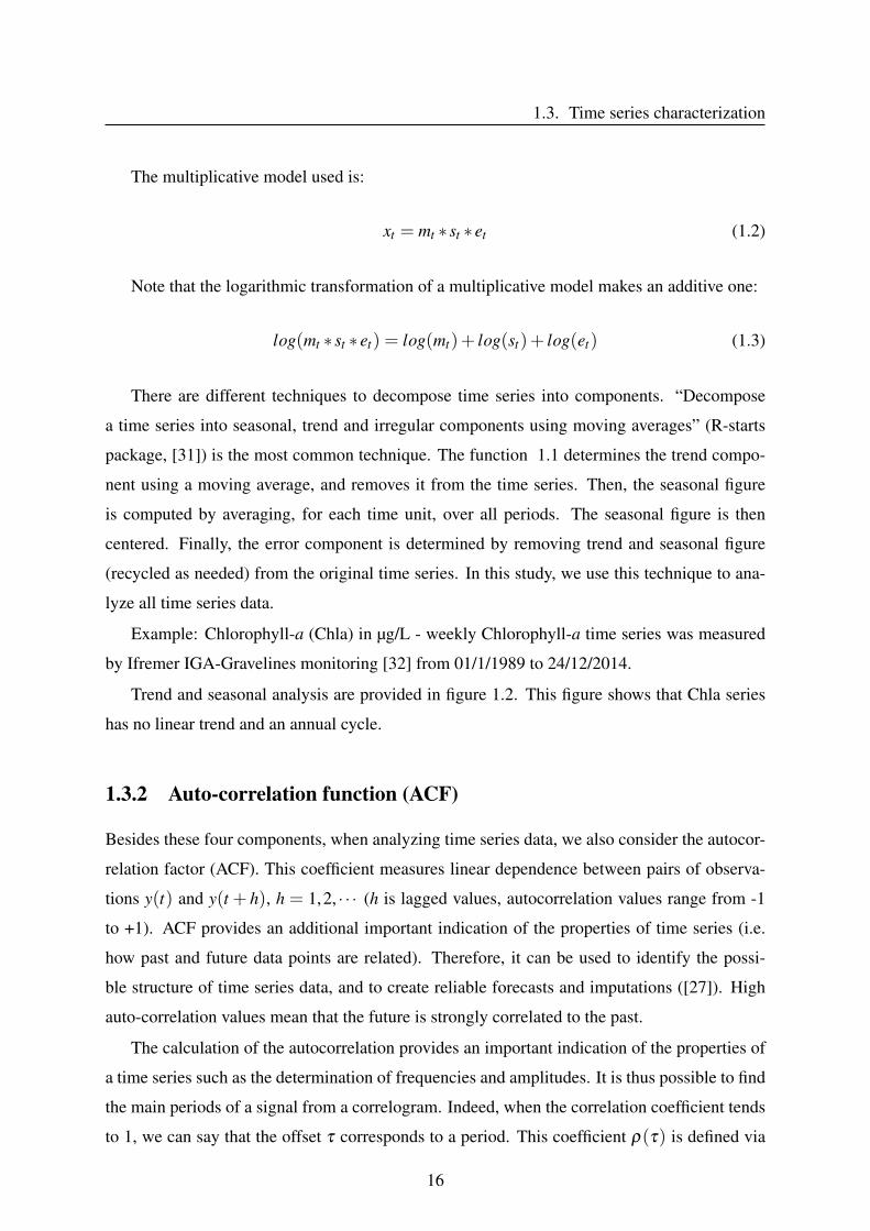
There are different techniques to decompose time series into components. “Decompose
a time series into seasonal, trend and irregular components using moving averages” (R-starts
package, [31]) is the most common technique. The function 1.1 determines the trend compo-
nent using a moving average, and removes it from the time series. Then, the seasonal figure
is computed by averaging, for each time unit, over all periods. The seasonal figure is then
centered. Finally, the error component is determined by removing trend and seasonal figure
(recycled as needed) from the original time series. In this study, we use this technique to ana-
lyze all time series data.
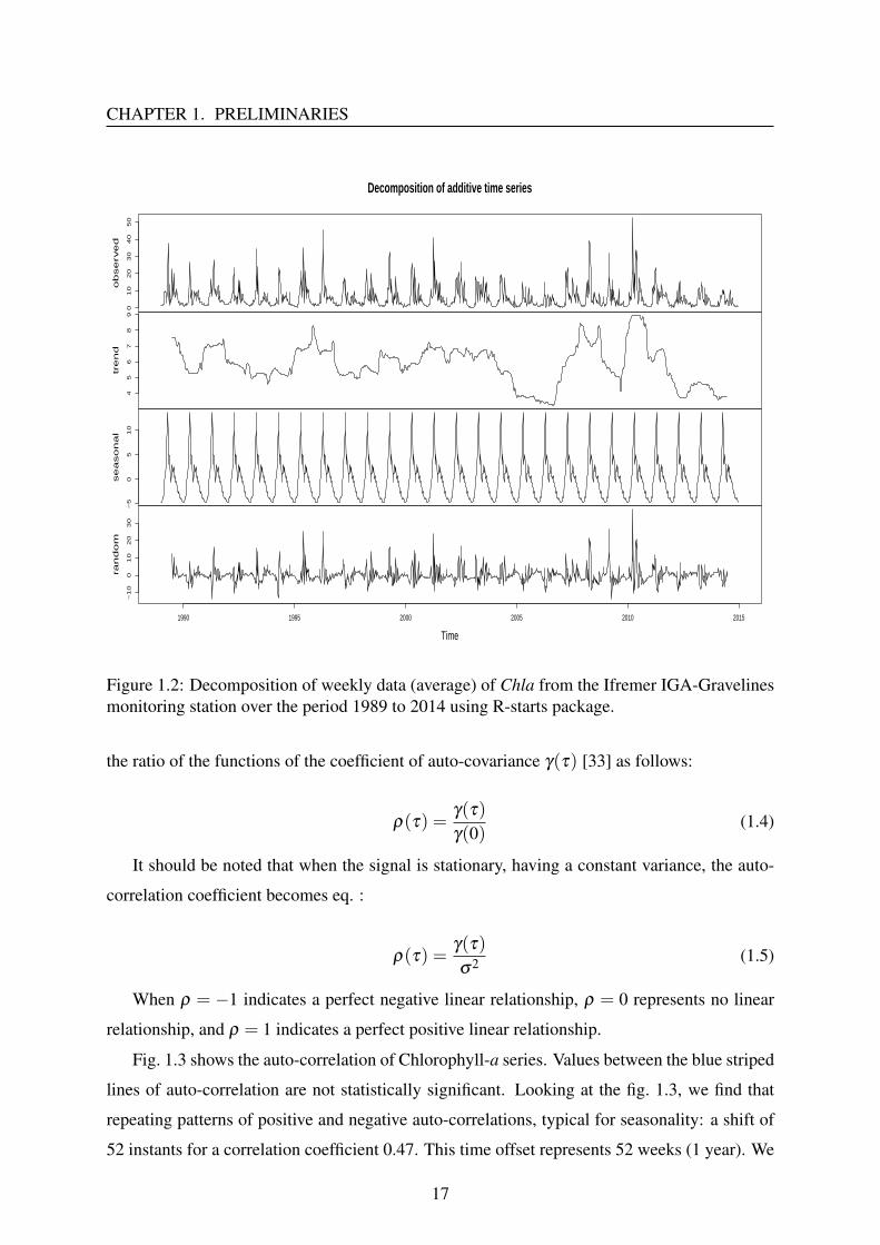
Example: Chlorophyll-a (Chla) in µg/L - weekly Chlorophyll-a time series was measured
by Ifremer IGA-Gravelines monitoring [32] from 01/1/1989 to 24/12/2014.
Trend and seasonal analysis are provided in figure 1.2. This figure shows that Chla series
has no linear trend and an annual cycle.
1.3.2 Auto-correlation function (ACF)
Besides these four components, when analyzing time series data, we also consider the autocor-
relation factor (ACF). This coefficient measures linear dependence between pairs of observa-
tions y(t) and y(t + h), h = 1,2, · · · (h is lagged values, autocorrelation values range from -1
to +1). ACF provides an additional important indication of the properties of time series (i.e.
how past and future data points are related). Therefore, it can be used to identify the possi-
ble structure of time series data, and to create reliable forecasts and imputations ([27]). High
auto-correlation values mean that the future is strongly correlated to the past.
The calculation of the autocorrelation provides an important indication of the properties of
a time series such as the determination of frequencies and amplitudes. It is thus possible to find
the main periods of a signal from a correlogram. Indeed, when the correlation coefficient tends
to 1, we can say that the offset τ corresponds to a period. This coefficient ρ(τ) is defined via
16
CHAPTER 1. PRELIMINARIES0
10
20
30
40
50
ob
se
rve
d
45
67
89
tre
nd
−5
05
10
se
aso
na
l
−1
00
10
20
30
1990 1995 2000 2005 2010 2015
ran
do
m
Time
Decomposition of additive time series
Figure 1.2: Decomposition of weekly data (average) of Chla from the Ifremer IGA-Gravelinesmonitoring station over the period 1989 to 2014 using R-starts package.
the ratio of the functions of the coefficient of auto-covariance γ(τ) [33] as follows:
ρ(τ) =γ(τ)
γ(0)(1.4)
It should be noted that when the signal is stationary, having a constant variance, the auto-
correlation coefficient becomes eq. :
ρ(τ) =γ(τ)
σ2 (1.5)
When ρ = −1 indicates a perfect negative linear relationship, ρ = 0 represents no linear
relationship, and ρ = 1 indicates a perfect positive linear relationship.
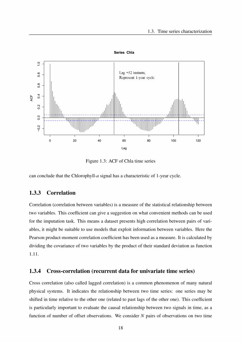
Fig. 1.3 shows the auto-correlation of Chlorophyll-a series. Values between the blue striped
lines of auto-correlation are not statistically significant. Looking at the fig. 1.3, we find that
repeating patterns of positive and negative auto-correlations, typical for seasonality: a shift of
52 instants for a correlation coefficient 0.47. This time offset represents 52 weeks (1 year). We
17
1.3. Time series characterization
Figure 1.3: ACF of Chla time series
can conclude that the Chlorophyll-a signal has a characteristic of 1-year cycle.
1.3.3 Correlation
Correlation (correlation between variables) is a measure of the statistical relationship between
two variables. This coefficient can give a suggestion on what convenient methods can be used
for the imputation task. This means a dataset presents high correlation between pairs of vari-
ables, it might be suitable to use models that exploit information between variables. Here the
Pearson product-moment correlation coefficient has been used as a measure. It is calculated by
dividing the covariance of two variables by the product of their standard deviation as function
1.11.
1.3.4 Cross-correlation (recurrent data for univariate time series)
Cross correlation (also called lagged correlation) is a common phenomenon of many natural
physical systems. It indicates the relationship between two time series: one series may be
shifted in time relative to the other one (related to past lags of the other one). This coefficient
is particularly important to evaluate the causal relationship between two signals in time, as a
function of number of offset observations. We consider N pairs of observations on two time
18
CHAPTER 1. PRELIMINARIES
series xt and yt , with h is the lag. Following Chatfield [33], the cross-covariance function is
computed as:
cxy(h) =1N
N−h
∑t=1
(xt− x)(yt+h− y),h = 0,1, · · · ,N−1 (1.6)
or
cxy(h) =1N
N
∑t=1−h
(xt− x)(yt+h− y),h = −1,−2, · · · ,−(N−1) (1.7)
where x and y are the means of xt and yt respectively.
This cross correlation measure can be calculated by obtaining the covariance between two
time series, and normalizing it with respect to the standard deviations of both time series.
rxy(h) =cxy(h)√
cxx(0)cyy(0)(1.8)
with cxx and cyy are the variances of xt and yt .
Two terms of “lead” and “lag” relationships are used to refer to the cross-correlation func-
tion as described by equations 1.6 or 1.7. The equation 1.6 means that xt is shifted h samples
back in time relative to yt . In this case xt is said to “lead” yt or yt is said to “lag” xt . The
equation 1.7 displays the reverse situation.
1.4 Experiments protocol
This part is designed to validate our proposed approaches and to compare with published meth-
ods for the imputation task. In this study, we deal with large missing values in two type of data:
the first type is univariate time series, while the second one is uncorrelated multivariate time
series. In experiments of univariate data, six imputation methods are considered viz., na.interp,
na.locf, na.approx, na.aggregate, na.spline and DTWBI. Concerning experiments of multivari-
ate data, we investigate 8 methods including FSMUMI, Amelia, FcM, MI, MICE, missForest,
na.approx and DTWUMI. We compare these methods in terms of their efficiency performance,
that means the comparison of quantitative and visualization performance. In the following sec-
tions, we present the design of the experimental process and the criteria for evaluating methods.
19
1.4. Experiments protocol
1.4.1 Experimental process for the imputation task
This section introduces detailed descriptions for conducting experiments. The experiments are
carried out in order to compare the performance of our proposals with different imputation
methods for handling missing values. Indeed, evaluating the ability of imputation methods
cannot be done because the actual values are lacking. So we must produce artificial missing
data on complete time series to assess the performance of imputation approaches. In this study,
T-gap missing type is considered to perform the experiments. Depending on each application,
we create simulated gaps with different rates ranging from 1%, 2%, 3%, 4%, 5%, 7.5% and
10% of the complete signal.
Therefore, we use a technique comprising three steps to evaluate the results as follows:
• The 1st step: Create artificial missing data by deleting data values from full time series.
• The 2nd step: Apply the imputation algorithms previously mentioned to complete missing
data. The result of this step thus is time series containing imputed values.
• The 3rd step: Assess the performance of proposed methods and compare with published
algorithms. In this step, we evaluate the performance of each imputation method by
comparing the imputed values with the true values (the original full time series). We use
different performance indicators as defined in next section.
1.4.2 Measurements for evaluating imputation methods
In this study, the completion data and observed data are compared to assess the performance of
imputation methods. To do this, seven performance indicators are introduced including Simi-
larity (Sim), Normalized Mean Absolute Error (NMAE), Root Mean Squared Error (RMSE),
coefficient of determination (R2), FB (Fractional Bias), FSD (Fraction of Standard Deviation
and FA2. Depending on each application that we use some of these indices. The indicators are
computed as follows:
1. Similarity: defines the similar percentage between the imputed values (y) and the respec-
tive true values (x). It is calculated by:
Sim(y,x) =1T
T
∑i=1
1
1+ |yi−xi|max(x)−min(x)
(1.9)
20
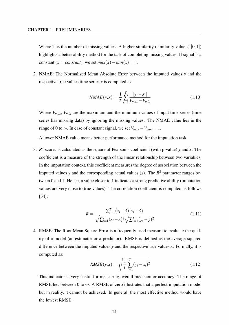
CHAPTER 1. PRELIMINARIES
Where T is the number of missing values. A higher similarity (similarity value ∈ [0,1])
highlights a better ability method for the task of completing missing values. If signal is a
constant (x = constant), we set max(x)−min(x) = 1.
2. NMAE: The Normalized Mean Absolute Error between the imputed values y and the
respective true values time series x is computed as:
NMAE(y,x) =1T
T
∑i=1
|yi− xi|Vmax−Vmin
(1.10)
Where Vmax, Vmin are the maximum and the minimum values of input time series (time
series has missing data) by ignoring the missing values. The NMAE value lies in the
range of 0 to ∞. In case of constant signal, we set Vmax−Vmin = 1.
A lower NMAE value means better performance method for the imputation task.
3. R2 score: is calculated as the square of Pearson’s coefficient (with p-value) y and x. The
coefficient is a measure of the strength of the linear relationship between two variables.
In the imputation context, this coefficient measures the degree of association between the
imputed values y and the corresponding actual values (x). The R2 parameter ranges be-
tween 0 and 1. Hence, a value closer to 1 indicates a strong predictive ability (imputation
values are very close to true values). The correlation coefficient is computed as follows
[34]:
R =∑
Ti=1(xi− x)(yi− y)√
∑Ti=1(xi− x)2
√∑
Ti=1(yi− y)2
(1.11)
4. RMSE: The Root Mean Square Error is a frequently used measure to evaluate the qual-
ity of a model (an estimator or a predictor). RMSE is defined as the average squared
difference between the imputed values y and the respective true values x. Formally, it is
computed as:
RMSE(y,x) =
√1T
T
∑i=1
(yi− xi)2 (1.12)
This indicator is very useful for measuring overall precision or accuracy. The range of
RMSE lies between 0 to ∞. A RMSE of zero illustrates that a perfect imputation model
but in reality, it cannot be achieved. In general, the most effective method would have
the lowest RMSE.
21

1.4. Experiments protocol
5. FSD (Fraction of Standard Deviation) of y and x is defined as follows:
FSD(y,x) = 2∗ |SD(y)−SD(x)|SD(y)+ SD(x)
(1.13)
This fraction indicates whether a method is acceptable or not (here SD stands for Stan-
dard Deviation). For the imputation task, if FSD is closer to 0, the imputation values are
closer to the real values.
6. FB - Fractional Bias between the imputed values y and the respective true values time
series x is defined by eq. 1.14. This parameter determines whether the imputation values
are overestimated or underestimated relatively to those observed. A model is considered
as perfect when its FB tends to zero, and as acceptable when −0.3≤ FB≤ 0.3
FB(y,x) = 2∗ mean(y)−mean(x)mean(y)+mean(x)
(1.14)
7. FA2: represents the fraction of data points that satisfied smoothing amplitude cover. It is
calculated as:
FA2(y,x) =length(0.5≤ y
x ≤ 2)length(x)
(1.15)
A model is considered perfect when FA2 is equal to 1.
Illustration
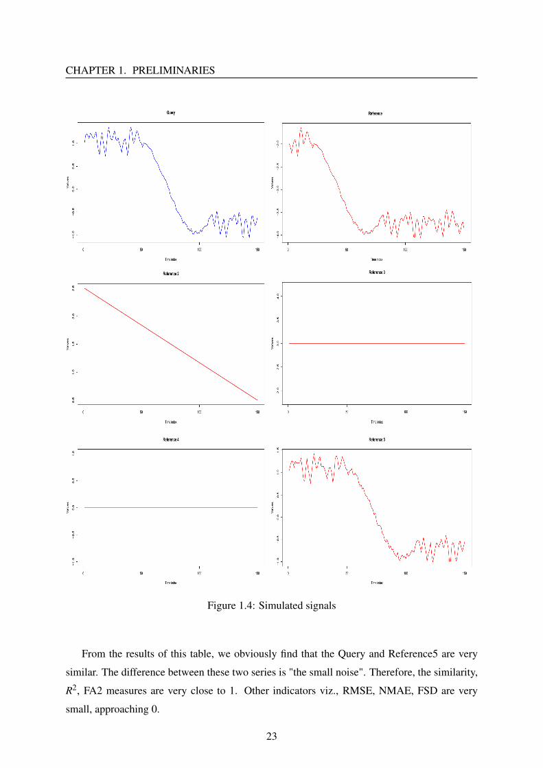
We illustrate the computation of these indicators by giving an example. Six different signals
are created (including: Query, Reference, Reference2, Reference3, Reference4 and Reference5
(see figure 1.4)) in the following way:
The Query is composed of three periods with three different sine waves.
The Reference is generated from the Query by changing its phase.
Three signals Reference2, Reference3 and Reference4 are just three constant lines.
The final series, Reference5, is yielded by adding small noise to the Query. The noise is
generated from a uniform distribution of the same size of the query between 0 and 0.1.
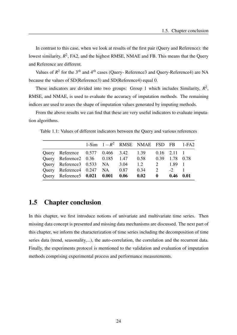
Table 1.1 shows the values of previous criteria between the Query and various references.
Zero value means that the two signals are similar.
22
CHAPTER 1. PRELIMINARIES
Figure 1.4: Simulated signals
From the results of this table, we obviously find that the Query and Reference5 are very
similar. The difference between these two series is "the small noise". Therefore, the similarity,
R2, FA2 measures are very close to 1. Other indicators viz., RMSE, NMAE, FSD are very
small, approaching 0.
23
1.5. Chapter conclusion
In contrast to this case, when we look at results of the first pair (Query and Reference): the
lowest similarity, R2, FA2, and the highest RMSE, NMAE and FB. This means that the Query
and Reference are different.
Values of R2 for the 3th and 4th cases (Query- Reference3 and Query-Reference4) are NA
because the values of SD(Reference3) and SD(Reference4) equal 0.
These indicators are divided into two groups: Group 1 which includes Similarity, R2,
RMSE, and NMAE, is used to evaluate the accuracy of imputation methods. The remaining
indices are used to asses the shape of imputation values generated by imputing methods.
From the above results we can find that these are very useful indicators to evaluate imputa-
tion algorithms.
Table 1.1: Values of different indicators between the Query and various references
1-Sim 1−R2 RMSE NMAE FSD FB 1-FA2
Query Reference 0.577 0.466 3.42 1.39 0.16 2.11 1Query Reference2 0.36 0.185 1.47 0.58 0.39 1.78 0.78Query Reference3 0.533 NA 3.04 1.2 2 1.89 1Query Reference4 0.247 NA 0.87 0.34 2 -2 1Query Reference5 0.021 0.001 0.06 0.02 0 0.46 0.01
1.5 Chapter conclusion
In this chapter, we first introduce notions of univariate and multivariate time series. Then
missing data concept is presented and missing data mechanisms are discussed. The next part of
this chapter, we inform the characterization of time series including the decomposition of time
series data (trend, seasonality,...), the auto-correlation, the correlation and the recurrent data.
Finally, the experiments protocol is mentioned to the validation and evaluation of imputation
methods comprising experimental process and performance measurements.
24
Chapter 2DTW-based imputation approach for
univariate time series
Contents2.1 Introduction . . . . . . . . . . . . . . . . . . . . . . . . . . . . . . . . . . 26
2.2 Literature review of Dynamic Time Warping . . . . . . . . . . . . . . . . 28
2.2.1 Classical DTW algorithm . . . . . . . . . . . . . . . . . . . . . . . 28
2.2.2 DDTW - Derivative Dynamic Time Warping . . . . . . . . . . . . . 32
2.2.3 AFBTW - Adaptive Feature Based Dynamic Time Warping . . . . . 33
2.2.4 Dissimilarity-based elastic matching . . . . . . . . . . . . . . . . . . 34
2.2.5 Dynamic Time Warping-D algorithm (DTW-D) . . . . . . . . . . . 35
2.2.6 Illustration . . . . . . . . . . . . . . . . . . . . . . . . . . . . . . . 35
2.3 Dynamic Time Warping-based imputation for univariate time series . . . 41
2.3.1 The proposed method - DTWBI . . . . . . . . . . . . . . . . . . . . 41
2.3.2 Validation procedure . . . . . . . . . . . . . . . . . . . . . . . . . . 44
2.3.3 Results and discussion . . . . . . . . . . . . . . . . . . . . . . . . . 47
2.3.4 Conclusion . . . . . . . . . . . . . . . . . . . . . . . . . . . . . . . 57
2.4 Comparison of various DTW versions for completing missing values inunivariate time series . . . . . . . . . . . . . . . . . . . . . . . . . . . . . 58
2.4.1 Introduction . . . . . . . . . . . . . . . . . . . . . . . . . . . . . . . 58
2.4.2 Imputation based on DTW metrics . . . . . . . . . . . . . . . . . . . 59
2.4.3 Data presentation . . . . . . . . . . . . . . . . . . . . . . . . . . . . 59
2.4.4 Results and discussion . . . . . . . . . . . . . . . . . . . . . . . . . 60
2.4.5 Conclusion . . . . . . . . . . . . . . . . . . . . . . . . . . . . . . . 64
2.5 Chapter conclusion . . . . . . . . . . . . . . . . . . . . . . . . . . . . . . 66
25
2.1. Introduction
In this chapter, we present a detailed methodology to impute missing values in univari-
ate time series based on combining the shape-feature extraction and Dynamic Time Warping
(DTW) algorithms. Firstly, it is important to understand the meaning and context of the ap-
plied approach, so they are introduced in Section 2.1. Next in Section 2.2, we present the main
theoretical background of DTW method and several of its variants. Then, in Section 2.3.1 we
describe our approach for univariate time series imputation. Sections 2.3.2 and 2.3.3 are to
validate the proposed method and to compare with state-of-the-art approaches. The next part
2.4, we perform a comparison of different DTW versions for the imputation of univariate time
series.
2.1 Introduction
Time series with missing values occur in almost domains of applied sciences. These missing
data may occur for a variety of reasons, for instance during maintenance, failure of measuring
instruments, data transmission problem etc. This is particularly the case for marine samples
([1], [2]). Furthermore, most time series analysis algorithms and most statistical softwares are
not designed to handle data with missing values. They often require complete data. However,
the regularization of time series makes it possible to complete missing values [35]. For low fre-
quency systems with monthly sampling, it is simple to apply a linear or polynomial regression
or moving average to fill in the series. Problems arise when completing missing values of high
frequency systems with quickly dynamics change.
For example, the MAREL-Carnot dataset, sampling frequency every 20 minutes, missing
values are 72 points for one day, 504 points for a week, and 2,200 points for a month. In this
case, the size of consecutive missing values (also called gap) is large. Example, the pH signal
has 131,472 observations of which 72.78% are available values. It contains 3,392 isolated
missing values and many consecutive missing data. The size of these gaps varies from one hour
to few months; the largest gap is a 16,843 points corresponding to 234 days (approximately 8
months). Single holes and gaps having T < tide duration-holes (807 missing points) could be
easily replaced by local averages. For the other gaps, the phytoplankton bloom dynamics or
composition changes too fast to use linear or spline imputation method.
In addition, collected data always contain noise due to high frequency, thus completion
process becomes more complex. Other classical solution consists in ignoring missing data
26
CHAPTER 2. DTW-BASED IMPUTATION APPROACH FOR UNIVARIATE TIMESERIES
or listwise deletion. But it is easy to imagine that this drastic solution may lead to serious
problems, especially for time series data (the considered values depend on the past values).
The first potential consequence of this method is information loss which could lose efficiency
([36]). The second consequence is about the systematic differences between observed and
unobserved data that leads to biased and unreliable results ([4]).
Therefore, it is crucial to propose a new technique to estimate missing values. One prospec-
tive approach to solve missing data problems is the adoption of imputation techniques ([5]).
These techniques should ensure that the obtained results are efficient (having minimal standard
errors) and reliable (effective, curve-shape respect).
In the literature, regarding imputation methods, a large number of successful approaches
have been proposed for completing missing data. For multivariate time series, efficient impu-
tation algorithms estimate missing values based on the values of other variables (correlations
between variables). However, handling missing values within univariate time series data dif-
fers from multivariate time series techniques. We must only rely on the available values of this
unique variable to estimate the incomplete values of the time series. Moritz et al. [27] showed
that imputing univariate time series data is a particularly challenging task.
Fewer studies are devoted to the imputation task for univariate time series. Allison [37] and
Bishop [38] proposed to simply substitute the mean or the median of available values to each
missing value. These simple algorithms provide the same result for all missing values leading
to bias result and to undervalue standard error ([39], [40]). Other imputation techniques for
univariate time series are linear interpolation, spline interpolation and the nearest neighbor in-
terpolation. These techniques were studied for missing data imputation in air quality datasets
([5]). The results showed that univariate methods are dependent upon the size of the gap: the
larger gap, the less effective technique. Walter et al. ([41]) carried out a performance compar-
ison of three methods for univariate time series, namely, ARIMA (Autoregressive Integrated
Moving Average), SARIMA (Seasonal ARIMA), and linear regression. The linear regression
method is more efficient and effective than the other two methods, only when rearranging the
data in periods. This study treated non-stationary seasonal time series data but it did not take
into account series without seasonality. Chiewchanwattana et al. proposed the Varied-Window
Similarity Measure (VWSM) algorithm ([42]). This method is better than the spline interpola-
tion, the multiple imputation, and the optimal completion strategy fuzzy c-means algorithms.
However, this research only focused on filling one isolated missing value, but did not consider
sub-sequence missing. Moritz et al. [27] performed an overview about univariate time series
27
2.2. Literature review of Dynamic Time Warping
imputation comparing six imputation methods. Nevertheless, this study only considered the
MCAR type.
Dynamic Time Warping (DTW) [7] is an effective and well-known method for measuring
similarity between two linear/nonlinear time series. The success of DTW in data mining [8],
information retrieval and pattern recognition [9, 10, 11] leads us to study its ability to complete
missing values in time series. In addition, taking advantage of available values to estimate the
missing values makes it possible to reconstruct data with more plausible values. Thus, the aim
of this chapter is to propose an algorithm to fill large gap(s) in univariate time series based
on Dynamic Time Warping ([7]) by exploiting the information of available values. We do not
deal with all the missing data over the entire series, but we focus on each large gap where
series-shape change could occur over the duration of this large gap.
Further, the distribution of missing values or entire signal could be very difficult to estimate,
so it is necessary to make some assumptions. Our approach makes an assumption that the
information on missing values exists within the univariate time series and takes into account
the time series characteristics.
Here, the main focus of this chapter is to investigate and propose a new algorithm for
completing large gap based on DTW method. Therefrom, we first introduce and discuss the
main ideas of Dynamic Time Warping approach and then summarize several modifications of
DTW.
2.2 Literature review of Dynamic Time Warping
2.2.1 Classical DTW algorithm
In time series analysis, finding out the similarity between two time series is a vital task for
numerous applications of time series. However, how do we define the similarity of two se-
quences (i.e time series)? And how do we find similar sequences quickly in a large databases
with different type of data format? Euclidean distance is the most popular measure that allows
to determine similarity and to index between two time series. But this distance is a very brittle
and it cannot index time series accurately with two different time phases. So we need a method
that permits to shift elastically on the time axis, and to contain sequences that are similar, but
out of time phase.
Dynamic Time Warping or elastic matching was initially proposed to recognize spoken
28
CHAPTER 2. DTW-BASED IMPUTATION APPROACH FOR UNIVARIATE TIMESERIES
words [7], and then it has been widely used in many applied applications like pattern recog-
nition [9, 10], shape retrieval [43, 44], gene expression [45], and so on. Unlike the Euclidean
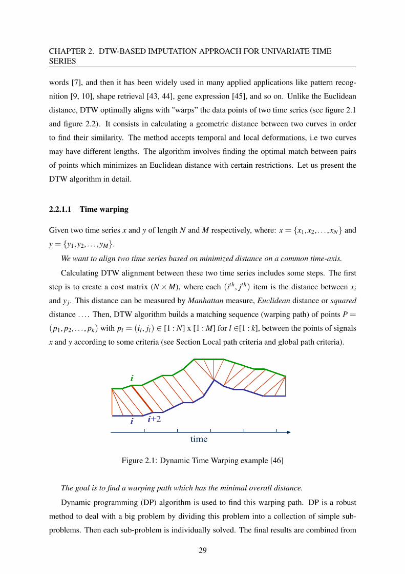
distance, DTW optimally aligns with "warps” the data points of two time series (see figure 2.1
and figure 2.2). It consists in calculating a geometric distance between two curves in order
to find their similarity. The method accepts temporal and local deformations, i.e two curves
may have different lengths. The algorithm involves finding the optimal match between pairs
of points which minimizes an Euclidean distance with certain restrictions. Let us present the
DTW algorithm in detail.
2.2.1.1 Time warping
Given two time series x and y of length N and M respectively, where: x = {x1,x2, . . . ,xN} and
y = {y1,y2, . . . ,yM}.
We want to align two time series based on minimized distance on a common time-axis.
Calculating DTW alignment between these two time series includes some steps. The first
step is to create a cost matrix (N×M), where each (ith, jth) item is the distance between xi
and y j. This distance can be measured by Manhattan measure, Euclidean distance or squared
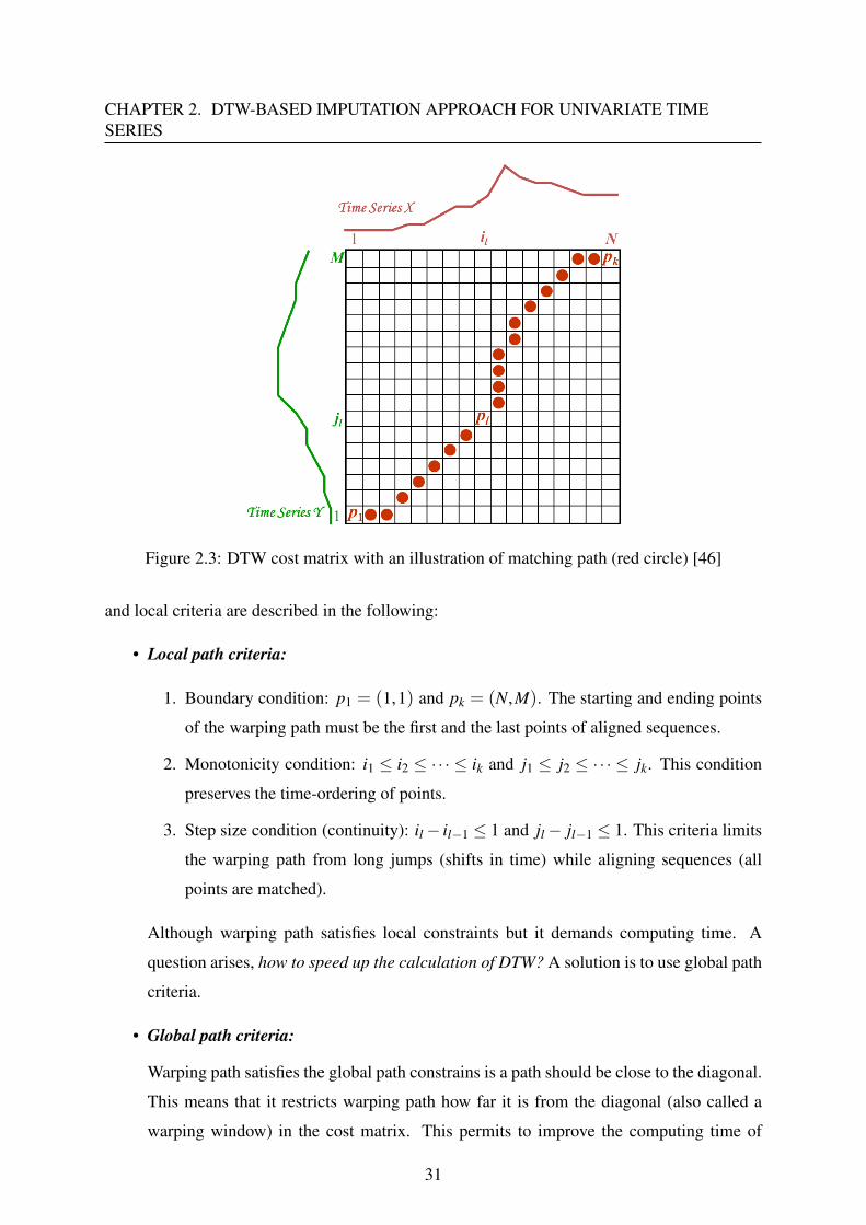
distance . . . . Then, DTW algorithm builds a matching sequence (warping path) of points P =
(p1, p2, . . . , pk) with pl = (il , jl) ∈ [1 : N] x [1 : M] for l ∈[1 : k], between the points of signals
x and y according to some criteria (see Section Local path criteria and global path criteria).
Figure 2.1: Dynamic Time Warping example [46]
The goal is to find a warping path which has the minimal overall distance.
Dynamic programming (DP) algorithm is used to find this warping path. DP is a robust
method to deal with a big problem by dividing this problem into a collection of simple sub-
problems. Then each sub-problem is individually solved. The final results are combined from
29
2.2. Literature review of Dynamic Time Warping
Figure 2.2: Euclidean example. Note that while the two sequences have an overall similarshape, they are not aligned in the time axis. Euclidean distance, which assumes the ith point inone sequence is aligned with the ith point in the other, will produce a pessimistic dissimilaritymeasure. The nonlinear Dynamic Time Warped alignment allows a more intuitive distancemeasure to be calculated [46]
all solutions to resolve the given problem. The next time, if the same sub-problem occurs, it
will be simple to look up previously computed solution instead of recalculating its result.
DTW uses the dynamic programming equation (2.1) to determine dist(i, j) - the cost matrix.
The equation (2.1) can be considered as a symmetric formulation, because both points around
the diagonal of the considered point have equal weights.
dist(i, j) = d(xi,y j)+min{dist(i−1, j−1),dist(i−1, j),dist(i, j−1)} (2.1)
The next step, the warping path between time series is found by using the cost matrix which
is filled by accumulated distances (defined by eq.2.1). Figure 2.3 shows the DTW process to
find the warping path between x and y time series. Back-tracking the cost matrix, the warping
path can be retrieved by applying a greedy method. Searching the warping path begins from
dist(N,M) and backtracks to the bottom left, with the assessment of all the adjacent cells from
left, down, diagonally. If one of these adjacent cells has the smallest value, it will be added to
the starting point of the warping path until dist(1,1) is reached.
Many warping paths can be generated from the equation (2.1), so in order to find the optimal
warping path from these achievable warping paths, some criteria (constraints) must be satisfied.
These constraints make it possible to reduce the search space for warping paths and to increase
the ability of the DTW algorithm. There are two types of constraints: the first one is local
criteria and the other one is global constraints. Local constraints perform slopes of the warping
path (local path) so this allows to calculate the accurate path. Global constraints make less the
search space for warping paths, and enhance the efficiency of DTW algorithm. These global
30
CHAPTER 2. DTW-BASED IMPUTATION APPROACH FOR UNIVARIATE TIMESERIES
Figure 2.3: DTW cost matrix with an illustration of matching path (red circle) [46]
and local criteria are described in the following:
• Local path criteria:
1. Boundary condition: p1 = (1,1) and pk = (N,M). The starting and ending points
of the warping path must be the first and the last points of aligned sequences.
2. Monotonicity condition: i1 ≤ i2 ≤ ·· · ≤ ik and j1 ≤ j2 ≤ ·· · ≤ jk. This condition
preserves the time-ordering of points.
3. Step size condition (continuity): il− il−1 ≤ 1 and jl− jl−1 ≤ 1. This criteria limits
the warping path from long jumps (shifts in time) while aligning sequences (all
points are matched).
Although warping path satisfies local constraints but it demands computing time. A
question arises, how to speed up the calculation of DTW? A solution is to use global path
criteria.
• Global path criteria:
Warping path satisfies the global path constrains is a path should be close to the diagonal.
This means that it restricts warping path how far it is from the diagonal (also called a
warping window) in the cost matrix. This permits to improve the computing time of
31
2.2. Literature review of Dynamic Time Warping
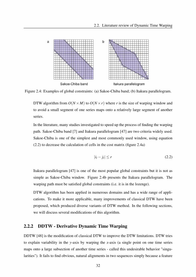
Figure 2.4: Examples of global constraints: (a) Sakoe-Chiba band; (b) Itakura parallelogram.
DTW algorithm from O(N×M) to O(N× r) where r is the size of warping window and
to avoid a small segment of one series maps onto a relatively large segment of another
series.
In the literature, many studies investigated to speed up the process of finding the warping
path. Sakoe-Chiba band [7] and Itakura parallelogram [47] are two criteria widely used.
Sakoe-Chiba is one of the simplest and most commonly used window, using equation
(2.2) to decrease the calculation of cells in the cost matrix (figure 2.4a)
|il− jl| ≤ r (2.2)
Itakura parallelogram [47] is one of the most popular global constraints but it is not as
simple as Sakoe-Chiba window. Figure 2.4b presents the Itakura parallelogram. The
warping path must be satisfied global constraints (i.e. it is in the lozenge).
DTW algorithm has been applied in numerous domains and has a wide range of appli-
cations. To make it more applicable, many improvements of classical DTW have been
proposed, which produced diverse variants of DTW method. In the following sections,
we will discuss several modifications of this algorithm.
2.2.2 DDTW - Derivative Dynamic Time Warping
DDTW [48] is the modification of classical DTW to improve the DTW limitations. DTW tries
to explain variability in the y-axis by warping the x-axis (a single point on one time series
maps onto a large subsection of another time series - called this undesirable behavior "singu-
larities"). It fails to find obvious, natural alignments in two sequences simply because a feature
32
CHAPTER 2. DTW-BASED IMPUTATION APPROACH FOR UNIVARIATE TIMESERIES
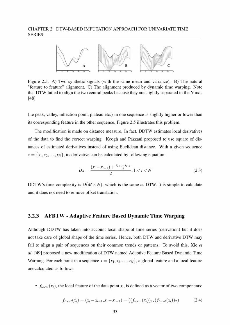
Figure 2.5: A) Two synthetic signals (with the same mean and variance). B) The natural"feature to feature" alignment. C) The alignment produced by dynamic time warping. Notethat DTW failed to align the two central peaks because they are slightly separated in the Y-axis[48]
(i.e peak, valley, inflection point, plateau etc.) in one sequence is slightly higher or lower than
its corresponding feature in the other sequence. Figure 2.5 illustrates this problem.
The modification is made on distance measure. In fact, DDTW estimates local derivatives
of the data to find the correct warping. Keogh and Pazzani proposed to use square of dis-
tances of estimated derivatives instead of using Euclidean distance. With a given sequence
x = {x1,x2, . . . ,xN}, its derivative can be calculated by following equation:
Dx =(xi− xi−1)+
xi+1−xi−12
2,1 < i < N (2.3)
DDTW’s time complexity is O(M×N), which is the same as DTW. It is simple to calculate
and it does not need to remove offset translation.
2.2.3 AFBTW - Adaptive Feature Based Dynamic Time Warping
Although DDTW has taken into account local shape of time series (derivation) but it does
not take care of global shape of the time series. Hence, both DTW and derivative DTW may
fail to align a pair of sequences on their common trends or patterns. To avoid this, Xie et
al. [49] proposed a new modification of DTW named Adaptive Feature Based Dynamic Time
Warping. For each point in a sequence x = {x1,x2, . . . ,xN}, a global feature and a local feature
are calculated as follows:
• flocal(xi), the local feature of the data point xi, is defined as a vector of two components:
flocal(xi) = (xi− xi−1,xi− xi+1) = (( flocal(xi))1, ( flocal(xi))2) (2.4)
33
2.2. Literature review of Dynamic Time Warping
• Global feature of a data point xi:
fglobal(xi) = (xi−i−1
∑k=1
xk
i−1,xi−
N
∑k=i+1
xk
N− i) = (( fglobal(xi))1, ( fglobal(xi))2) (2.5)
In this method, instead of using Euclidean distance between xi and y j, the authors pro-
posed to use a distance calculating as follows:
dist(xi,y j) = w1 distlocal(xi,y j)+w2 distglobal(xi,y j) (2.6)
where dist(xi,y j) is the overall distance between xi and y j. w1 and w2 weights are used
to adjust the percentage influence of local and global criteria, and w1+w2 = 1,0≤ w1 ≤1,0≤ w1 ≤ 1. distlocal(xi,y j) and distglobal(xi,y j) are distances between xi and y j based
on their local features and global features, and they are computed in the following:
distlocal(xi,y j) = |( flocal(xi))1− ( flocal(y j))1|+ |( flocal(xi))2− ( flocal(y j))2| (2.7)
distglobal(xi,y j) = |( fglobal(xi))1− ( fglobal(y j))1|+ |( fglobal(xi))2− ( fglobal(y j))2|(2.8)
2.2.4 Dissimilarity-based elastic matching
In the previous studies, the cost function provided by DTW, DDTW and AFBDTW is a relative
measure, which cannot be easily interpreted by itself. It is a mean distance, which depends on
the intensities of both signals. In order to make the response similar to the one of a human
expert, Caillault et al. [50] proposed a bounded measure of dissimilarity, between 0 and 1, that
adapts the DTW matching cost. The authors defined a dissimilarity s, replacing the Euclidean
distance d, as a ratio of distances:
s(xil ,y jl ) =d(xil ,y jl )
max{d(xil ,0),d(y jl ,0)}(2.9)
where x = {x1,x2, . . . ,xN}, y = {y1,y2, . . . ,yM} and P = {(il , jl), l = 1 . . .k, il = 1 . . .N, jl =
1 . . .M} is a matching path between the points of x and y signals.
In this work, an extended approach is also proposed allowing to calculate DTW distance on
34
CHAPTER 2. DTW-BASED IMPUTATION APPROACH FOR UNIVARIATE TIMESERIES
multidimensional signals (see [50] for more detail).
2.2.5 Dynamic Time Warping-D algorithm (DTW-D)
Chen et al. [51] proposed an other version of DTW devoted to applications of time series semi-
supervised learning. The authors exploited the difference/delta between DTW and Euclidean
Distance (ED) for the time series classification task. They showed that DTW-D provides better
discrimination than DTW through experiments. Given two time series x and y, DTW-D distance
is defined as follows:
DTW −D(x,y) = DTW (x,y)/(ED(x,y)+ ε) (2.10)
where ε is a very small positive number that is used to avoid divide-by-zero error.
2.2.6 Illustration
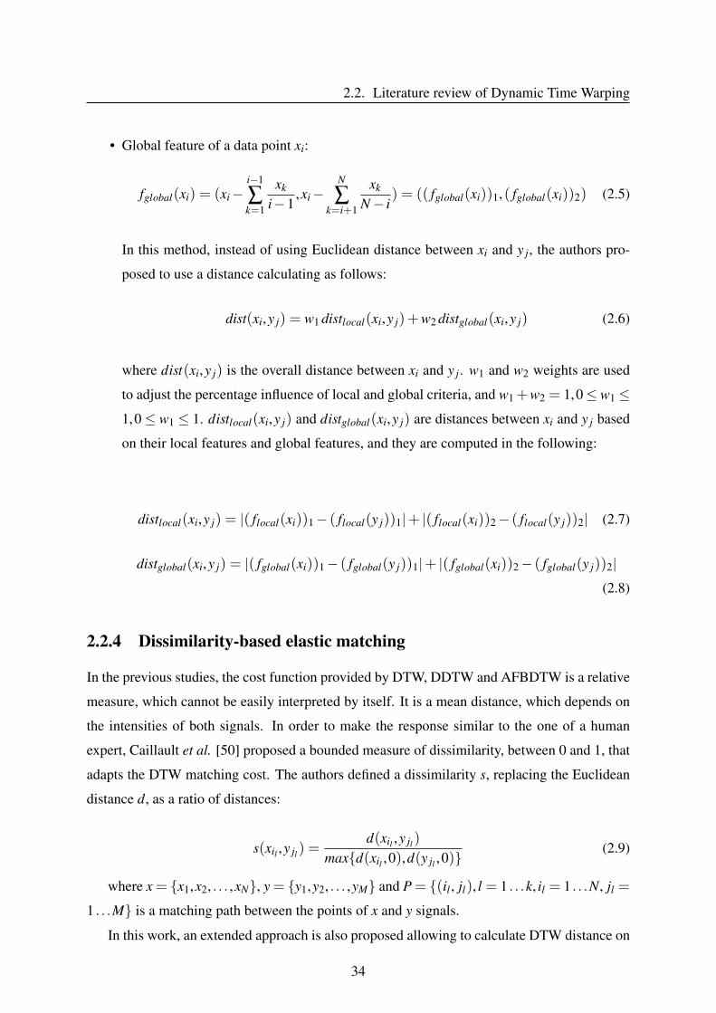
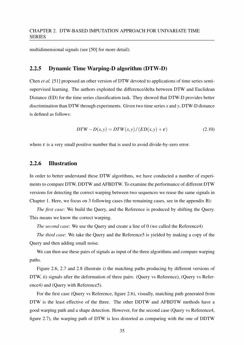
In order to better understand these DTW algorithms, we have conducted a number of experi-
ments to compare DTW, DDTW and AFBDTW. To examine the performance of different DTW
versions for detecting the correct warping between two sequences we reuse the same signals in
Chapter 1. Here, we focus on 3 following cases (the remaining cases, see in the appendix B):
The first case: We build the Query, and the Reference is produced by shifting the Query.
This means we know the correct warping.
The second case: We use the Query and create a line of 0 (we called the Reference4)
The third case: We take the Query and the Reference5 is yielded by making a copy of the
Query and then adding small noise.
We can then use these pairs of signals as input of the three algorithms and compare warping
paths.
Figure 2.6, 2.7 and 2.8 illustrate i) the matching paths producing by different versions of
DTW, ii) signals after the deformation of three pairs: (Query vs Reference), (Query vs Refer-
ence4) and (Query with Reference5).
For the first case (Query vs Reference, figure 2.6), visually, matching path generated from
DTW is the least effective of the three. The other DDTW and AFBDTW methods have a
good warping path and a shape detection. However, for the second case (Query vs Reference4,
figure 2.7), the warping path of DTW is less distorted as comparing with the one of DDTW
35
2.2. Literature review of Dynamic Time Warping
Figure 2.6: Query vs Reference
36
CHAPTER 2. DTW-BASED IMPUTATION APPROACH FOR UNIVARIATE TIMESERIES
Figure 2.7: Query vs Reference4
37
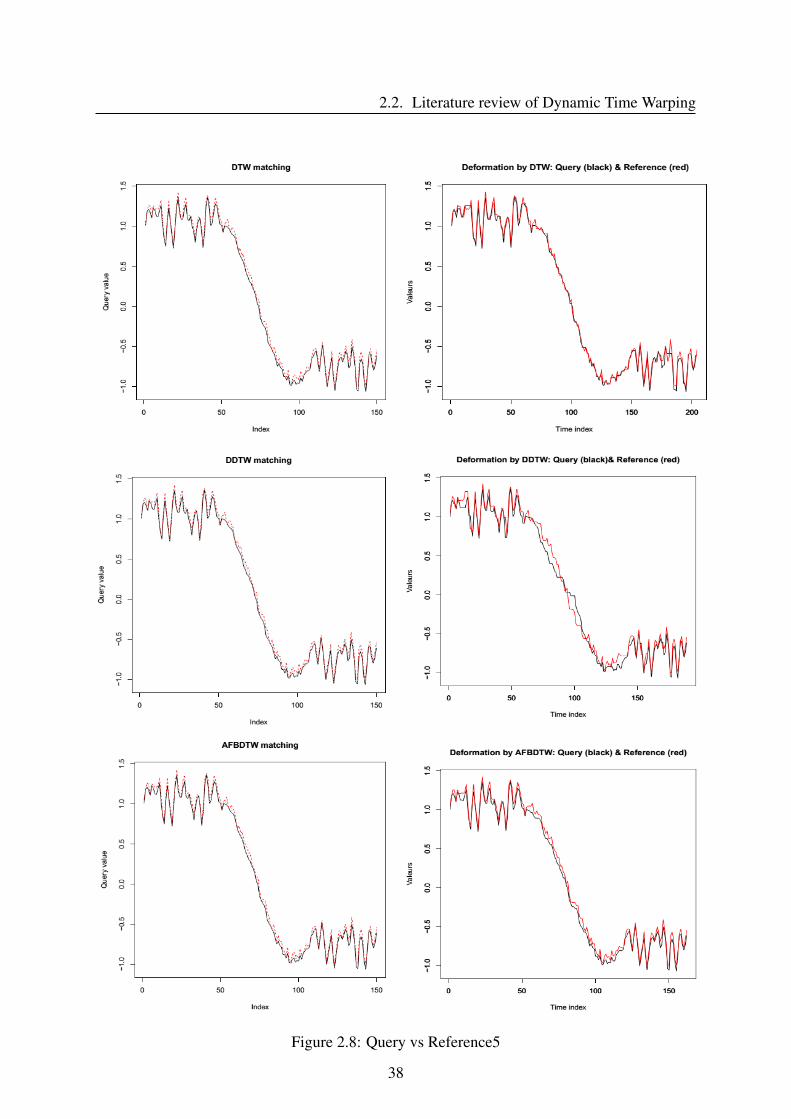
2.2. Literature review of Dynamic Time Warping
Figure 2.8: Query vs Reference5
38
CHAPTER 2. DTW-BASED IMPUTATION APPROACH FOR UNIVARIATE TIMESERIES
and AFBDTW. For the last case (Query with Reference5, figure 2.8), because the difference
between Query and Reference5 is very small. So we see the warping paths of all three methods
are very good. But when looking at deformation signals, it strongly shows that DTW has more
accurate matching than the two remaining cases.
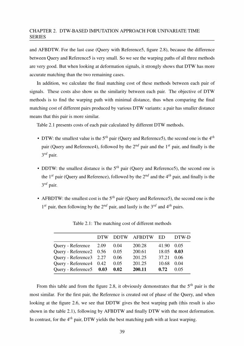
In addition, we calculate the final matching cost of these methods between each pair of
signals. These costs also show us the similarity between each pair. The objective of DTW
methods is to find the warping path with minimal distance, thus when comparing the final
matching cost of different pairs produced by various DTW variants: a pair has smaller distance
means that this pair is more similar.
Table 2.1 presents costs of each pair calculated by different DTW methods.
• DTW: the smallest value is the 5th pair (Query and Reference5), the second one is the 4th
pair (Query and Reference4), followed by the 2nd pair and the 1st pair, and finally is the
3rd pair.
• DDTW: the smallest distance is the 5th pair (Query and Reference5), the second one is
the 1st pair (Query and Reference), followed by the 2nd and the 4th pair, and finally is the
3rd pair.
• AFBDTW: the smallest cost is the 5th pair (Query and Reference5), the second one is the
1st pair, then following by the 2nd pair, and lastly is the 3rd and 4th pairs.
Table 2.1: The matching cost of different methods
DTW DDTW AFBDTW ED DTW-D
Query - Reference 2.09 0.04 200.28 41.90 0.05Query - Reference2 0.56 0.05 200.61 18.05 0.03Query - Reference3 2.27 0.06 201.25 37.21 0.06Query - Reference4 0.42 0.05 201.25 10.68 0.04Query - Reference5 0.03 0.02 200.11 0.72 0.05
From this table and from the figure 2.8, it obviously demonstrates that the 5th pair is the
most similar. For the first pair, the Reference is created out of phase of the Query, and when
looking at the figure 2.6, we see that DDTW gives the best warping path (this result is also
shown in the table 2.1), following by AFBDTW and finally DTW with the most deformation.
In contrast, for the 4th pair, DTW yields the best matching path with at least warping.
39
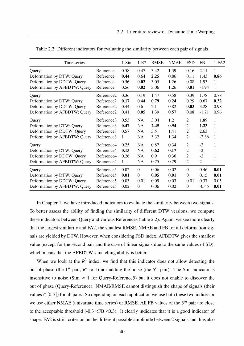
2.2. Literature review of Dynamic Time Warping
Table 2.2: Different indicators for evaluating the similarity between each pair of signals
Time series 1-Sim 1-R2 RMSE NMAE FSD FB 1-FA2
Query Reference 0.58 0.47 3.42 1.39 0.16 2.11 1Deformation by DTW: Query Reference 0.44 0.64 2.25 0.86 0.11 1.43 0.86Deformation by DDTW: Query Reference 0.56 0.02 3.05 1.26 0.08 1.93 1Deformation by AFBDTW: Query Reference 0.56 0.02 3.06 1.26 0.01 -1.94 1
Query Reference2 0.36 0.19 1.47 0.58 0.39 1.78 0.78Deformation by DTW: Query Reference2 0.17 0.44 0.79 0.24 0.29 0.67 0.32Deformation by DDTW: Query Reference2 0.44 0.6 2.1 0.82 0.03 3.28 0.98Deformation by AFBDTW: Query Reference2 0.41 0.05 1.39 0.57 0.08 -1.71 0.96
Query Reference3 0.53 NA 3.04 1.2 2 1.89 1Deformation by DTW: Query Reference3 0.47 NA 2.45 0.94 2 1.23 1Deformation by DDTW: Query Reference3 0.57 NA 3.5 1.41 2 2.63 1Deformation by AFBDTW: Query Reference3 1 NA 3.32 1.34 2 -2.36 1
Query Reference4 0.25 NA 0.87 0.34 2 -2 1Deformation by DTW: Query Reference4 0.13 NA 0.62 0.17 2 -2 1Deformation by DDTW: Query Reference4 0.26 NA 0.9 0.36 2 -2 1Deformation by AFBDTW: Query Reference4 1 NA 0.75 0.29 2 2 1
Query Reference5 0.02 0 0.06 0.02 0 0.46 0.01Deformation by DTW: Query Reference5 0.01 0 0.05 0.01 0 0.15 0.01Deformation by DDTW: Query Reference5 0.03 0.01 0.09 0.03 0.01 0.37 0.05Deformation by AFBDTW: Query Reference5 0.02 0 0.06 0.02 0 -0.45 0.01
In Chapter 1, we have introduced indicators to evaluate the similarity between two signals.
To better assess the ability of finding the similarity of different DTW versions, we compute
these indicators between Query and various References (table 2.2). Again, we see more clearly
that the largest similarity and FA2, the smallest RMSE, NMAE and FB for all deformation sig-
nals are yielded by DTW. However, when considering FSD index, AFBDTW gives the smallest
value (except for the second pair and the case of linear signals due to the same values of SD),
which means that the AFBDTW’s matching ability is better.
When we look at the R2 index, we find that this indicator does not allow detecting the
out of phase (the 1st pair, R2 ≈ 1) nor adding the noise (the 5th pair). The Sim indicator is
insensitive to noise (Sim ≈ 1 for Query-Reference5) but it does not enable to discover the
out of phase (Query-Reference). NMAE/RMSE cannot distinguish the shape of signals (their
values ∈ [0,3]) for all pairs. So depending on each application we use both these two indices or
we use either NMAE (univariate time series) or RMSE. All FB values of the 5th pair are close
to the acceptable threshold (-0.3 <FB <0.3). It clearly indicates that it is a good indicator of
shape. FA2 is strict criterion on the different possible amplitude between 2 signals and thus also
40
CHAPTER 2. DTW-BASED IMPUTATION APPROACH FOR UNIVARIATE TIMESERIES
makes it possible to assess well the similarity of shape (FA2≈ 0.99 for all cases of Reference5).
We can conclude that depending on the structure of each pair of signals, different versions
of DTW will produce the matching path with different deformation level.
2.3 Dynamic Time Warping-based imputation for
univariate time series
2.3.1 The proposed method - DTWBI
In this part, we present a new method for imputing missing values of univariate time series data
based on the combination of shape-feature extraction and DTW algorithms.
Given an incomplete time series x, with T - gap at position t (xi = NA, i = t : t + T − 1).
Here, we consider a large gap when T ≥ 6%N for small time series (N < 10,000) or when T is
larger than the known-process change.
The general architecture of our proposal DTWBI (Dynamic Time Warping-Based Impu-
tation) is shown in Figure 2.9. It involves 4 steps: 1- Building query, 2- Comparing sliding
window, 3- Selecting window, 4-Filling gap.
The proposed approach consists in finding the most similar sub-sequence (Qs) to a query
(Q) (Step 2-Comparing sliding window and step 3- Selecting window), with Q is the sub-
sequence before a gap of T size at position t (Q = x[t−T : t−1]) (Step 1-Building query), and
completes this gap by Q f s - the following sub-sequence of the Qs (Step 4-Filling the gap).
In this work, we always create the query with the same size of the considered gap in or-
der to look for the similar window having the same dynamics. Furthermore, the algorithm is
expandable by choosing a window after the gap. Here we build a query before the gap if its
position is in the second half of the signal otherwise after the gap. This ensures that there is
always enough data to search similar window.
To find the Qs similar sub-sequence, we use the principles of Dynamic Time Warping -
DTW ([7]), especially transformed from original data to Derivative Dynamic Time Warping -
DDTW data ([48]). The DDTW data are used because we can obtain information about the
shape of sequence ([48]). The dynamics and the shape of data before a gap are a key-point of
our method. The elastic matching is used to find a similar window to the Q query of T size in
the search database. Once the most similar window is identified, the following window will be
copied to the location of missing values. Fig. 2.10 describes the different steps of our approach.
41
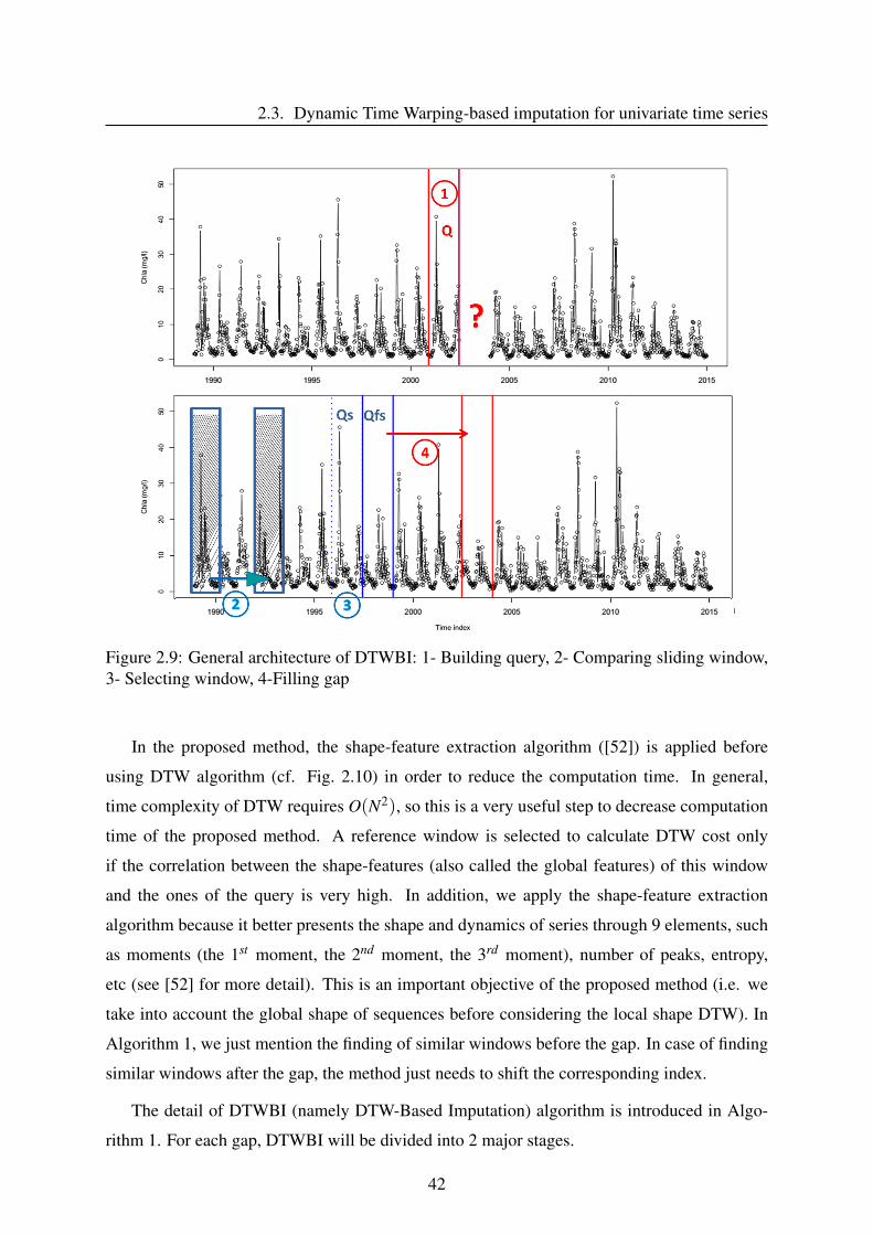
2.3. Dynamic Time Warping-based imputation for univariate time series
Figure 2.9: General architecture of DTWBI: 1- Building query, 2- Comparing sliding window,3- Selecting window, 4-Filling gap
In the proposed method, the shape-feature extraction algorithm ([52]) is applied before
using DTW algorithm (cf. Fig. 2.10) in order to reduce the computation time. In general,
time complexity of DTW requires O(N2), so this is a very useful step to decrease computation
time of the proposed method. A reference window is selected to calculate DTW cost only
if the correlation between the shape-features (also called the global features) of this window
and the ones of the query is very high. In addition, we apply the shape-feature extraction
algorithm because it better presents the shape and dynamics of series through 9 elements, such
as moments (the 1st moment, the 2nd moment, the 3rd moment), number of peaks, entropy,
etc (see [52] for more detail). This is an important objective of the proposed method (i.e. we
take into account the global shape of sequences before considering the local shape DTW). In
Algorithm 1, we just mention the finding of similar windows before the gap. In case of finding
similar windows after the gap, the method just needs to shift the corresponding index.
The detail of DTWBI (namely DTW-Based Imputation) algorithm is introduced in Algo-
rithm 1. For each gap, DTWBI will be divided into 2 major stages.
42
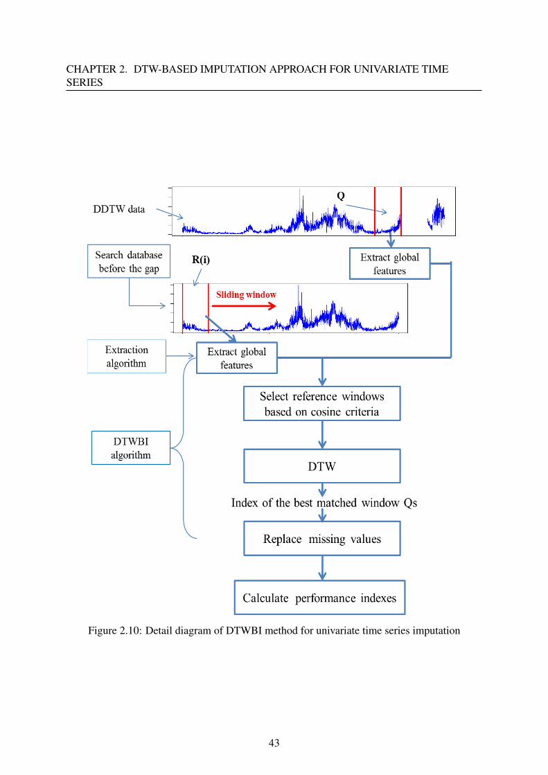
CHAPTER 2. DTW-BASED IMPUTATION APPROACH FOR UNIVARIATE TIMESERIES
Figure 2.10: Detail diagram of DTWBI method for univariate time series imputation
43
2.3. Dynamic Time Warping-based imputation for univariate time series
The first stage is to find a global threshold to determine two sub-sequences being similar
(Step 4: in Algorithm 1). This threshold is calculated as follows: after creating the query Q,
for each step_threshold, if the global shape between a reference window Ri and the query Q is
similar (this means that the consine value between global features of the two windows is greater
than θ_cos), we will calculate DTW-cost between Ri and Q. The DTW-threshold is estimated
as the minimum distance obtained from all sequences Ri analyzed with Q.
The second stage is to retrieve the most similar window to the query. Similarly to the first
stage, with each step_sim_win, we only compute DTW cost between a sliding reference Ri and
the query Q as the correlation condition is satisfied. We then compare this DTW cost to the
threshold to determine if this Ri reference is similar to the query Q. Ri reference and Q query
are considered similar if their DTW cost is less than the threshold. We thereafter select the
most similar window Qs with the minimum DTW cost of all the similar windows ( Step 5: in
Algorithm 1). Lastly, the gap is completed by the Q f s vector after the Qs.
2.3.2 Validation procedure
This part is designed to validate our proposal and compare with state-of-the-art methods of data
imputation (namely, na.interp, na.locf, na.approx, na.aggregate, na.spline). We assess these
methods in terms of their efficacy of accuracy and shape between actual data with completion
data using criteria for evaluation as defined in Chapter 1. In the following, we present the
datasets, univariate time series imputation methods, and experimental results.
2.3.2.1 Data presentation
In this study, we analyze 8 datasets in order to evaluate the performance of the proposed tech-
nique. Four datasets come from TSA package ([53]). These datasets are chosen because they
are usually used in the literature, including Airpassenger, Beersales, Google, and SP. Besides,
we also choose other datasets from various domains in different places:
1. Airpassenger - Monthly total international airline passengers from 01/1960 to 12/1971.
2. Beersales - Monthly beer sales in millions of barrels, from 01/1975 to 12/1990.
3. Google - Daily returns of the google stock from 08/20/04 to 09/13/06.
4. SP - Quarterly S&P Composite Index, 1936Q1 - 1977Q4.
44
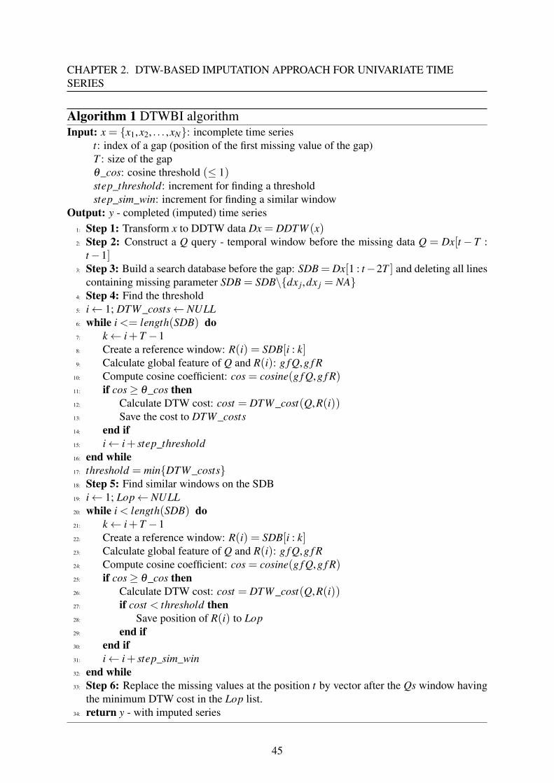
CHAPTER 2. DTW-BASED IMPUTATION APPROACH FOR UNIVARIATE TIMESERIES
Algorithm 1 DTWBI algorithmInput: x = {x1,x2, . . . ,xN}: incomplete time series
t: index of a gap (position of the first missing value of the gap)T : size of the gapθ_cos: cosine threshold (≤ 1)step_threshold: increment for finding a thresholdstep_sim_win: increment for finding a similar window
Output: y - completed (imputed) time series1: Step 1: Transform x to DDTW data Dx = DDTW (x)2: Step 2: Construct a Q query - temporal window before the missing data Q = Dx[t−T :
t−1]3: Step 3: Build a search database before the gap: SDB = Dx[1 : t−2T ] and deleting all lines
containing missing parameter SDB = SDB\{dx j,dx j = NA}4: Step 4: Find the threshold5: i← 1; DTW_costs← NULL6: while i <= length(SDB) do7: k← i+T −18: Create a reference window: R(i) = SDB[i : k]9: Calculate global feature of Q and R(i): g f Q,g f R
10: Compute cosine coefficient: cos = cosine(g f Q,g f R)11: if cos≥ θ_cos then12: Calculate DTW cost: cost = DTW_cost(Q,R(i))13: Save the cost to DTW_costs14: end if15: i← i+ step_threshold16: end while17: threshold = min{DTW_costs}18: Step 5: Find similar windows on the SDB19: i← 1; Lop← NULL20: while i < length(SDB) do21: k← i+T −122: Create a reference window: R(i) = SDB[i : k]23: Calculate global feature of Q and R(i): g f Q,g f R24: Compute cosine coefficient: cos = cosine(g f Q,g f R)25: if cos≥ θ_cos then26: Calculate DTW cost: cost = DTW_cost(Q,R(i))27: if cost < threshold then28: Save position of R(i) to Lop29: end if30: end if31: i← i+ step_sim_win32: end while33: Step 6: Replace the missing values at the position t by vector after the Qs window having
the minimum DTW cost in the Lop list.34: return y - with imputed series
45
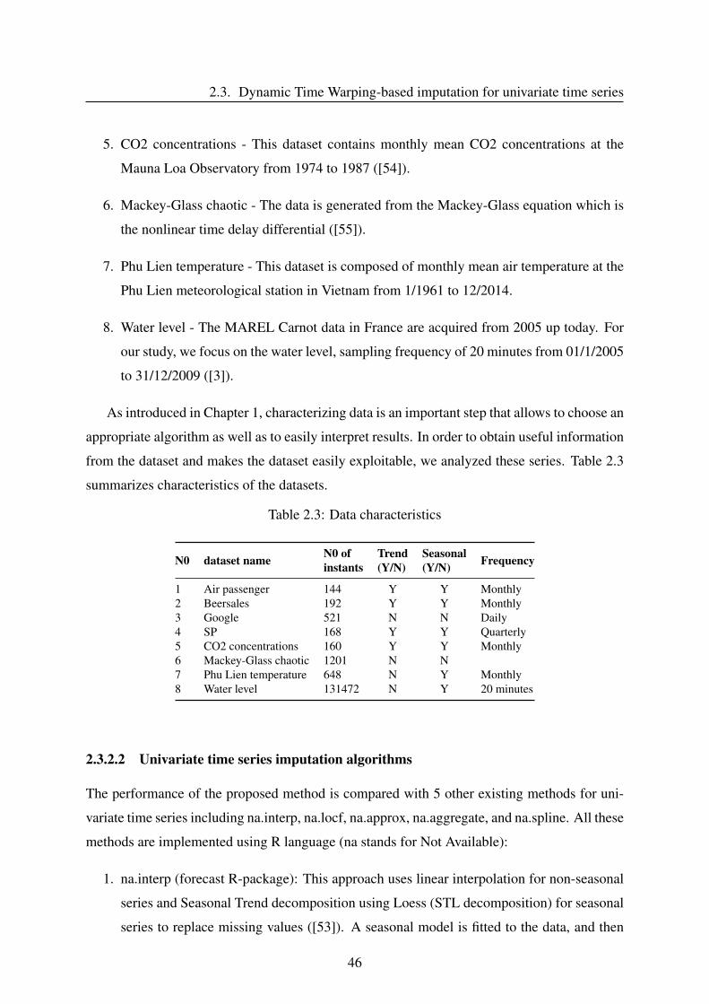
2.3. Dynamic Time Warping-based imputation for univariate time series
5. CO2 concentrations - This dataset contains monthly mean CO2 concentrations at the
Mauna Loa Observatory from 1974 to 1987 ([54]).
6. Mackey-Glass chaotic - The data is generated from the Mackey-Glass equation which is
the nonlinear time delay differential ([55]).
7. Phu Lien temperature - This dataset is composed of monthly mean air temperature at the
Phu Lien meteorological station in Vietnam from 1/1961 to 12/2014.
8. Water level - The MAREL Carnot data in France are acquired from 2005 up today. For
our study, we focus on the water level, sampling frequency of 20 minutes from 01/1/2005
to 31/12/2009 ([3]).
As introduced in Chapter 1, characterizing data is an important step that allows to choose an
appropriate algorithm as well as to easily interpret results. In order to obtain useful information
from the dataset and makes the dataset easily exploitable, we analyzed these series. Table 2.3
summarizes characteristics of the datasets.
Table 2.3: Data characteristics
N0 dataset name N0 ofinstants
Trend(Y/N)
Seasonal(Y/N) Frequency
1 Air passenger 144 Y Y Monthly2 Beersales 192 Y Y Monthly3 Google 521 N N Daily4 SP 168 Y Y Quarterly5 CO2 concentrations 160 Y Y Monthly6 Mackey-Glass chaotic 1201 N N7 Phu Lien temperature 648 N Y Monthly8 Water level 131472 N Y 20 minutes
2.3.2.2 Univariate time series imputation algorithms
The performance of the proposed method is compared with 5 other existing methods for uni-
variate time series including na.interp, na.locf, na.approx, na.aggregate, and na.spline. All these
methods are implemented using R language (na stands for Not Available):
1. na.interp (forecast R-package): This approach uses linear interpolation for non-seasonal
series and Seasonal Trend decomposition using Loess (STL decomposition) for seasonal
series to replace missing values ([53]). A seasonal model is fitted to the data, and then
46
CHAPTER 2. DTW-BASED IMPUTATION APPROACH FOR UNIVARIATE TIMESERIES
interpolation is made on the seasonally adjusted series, before re-seasonalizing. So, this
method is especially devoted to strong and clear seasonality data.
2. na.locf (last observation carried forward) (zoo R-package): This method replaces any
missing value by the most recent available value prior to it ([56]). This is one of the most
simple algorithm which takes into account characteristics of time series. Because in fact,
it has often a clear relation between a considered observation (at tn) and its previous one
(at tn−1), so this method is quite strong. For all data with daily sampling, this method
is suited: the value of the next day seems similar to its predecessor (for example daily
temperature). But it has disadvantages when there are large differences between observed
value at moment tn and its previous point at tn−1 (especially in the case of time series
having strong seasonality). In [57], the author pointed out that the mean and covariance
structure are usually distorted when using this method. Molenberghs et al. showed that
locf is generally biased even under MCAR ([58]).
In general, this method assumes that the outcome would not change after the last observed
value. Therefore, there has been no time effect since the last observed data.
3. na.approx (zoo R-package): This method is integrated in the zoo R-package. It use a
linear interpolation to estimate each missing value ([56]). The difference between this
method and na.interp is that na.interp takes into account the seasonal component and
na.approx does not take this. Therefore, with signals have no the seasonal factor, impu-
tation results of the two methods are the same.
4. na.aggregate (zoo R-package): This algorithm applies a generic function to replace each
NA with aggregated values. This allows to complete a NA by using the overall mean,
monthly means, etc ([56]). In our experiment, we use the overall mean. With this compu-
tation, na.agrregate does not exploit the characteristics of time series. In particular, this
method is not good when time series having a strong trend.
5. na.spline (zoo R-package): This algorithm uses a polynomial (cubic) interpolation to
complete missing data ([56]).
2.3.3 Results and discussion
For assessing the results, we apply the experiment protocol as previously defined in Chapter
1. In the present study, 5 missing data levels are considered on 8 datasets. When the size of
47
2.3. Dynamic Time Warping-based imputation for univariate time series
a dataset (number of instants of the dataset) is less than or equal to 10,000 samples, we create
gaps with different sizes: 6%, 7.5%, 10%, 12.5%, 15% of overall dataset size. In contrast,
when the size of a dataset is greater than 10,000 sampling points, gaps are built at rates 0.6%,
0.75%, 1%, 1.25%, and 1.5% of the dataset size (here the largest gap of the water level time
series is 1,972 missing values, corresponding to the missing rate 1.5%). For each missing rate,
the algorithms are conducted 10 times by randomly selecting the missing positions on the data.
We then run 50 iterations for each dataset.
Results are analyzed in two respects comprising quantitative performance and visual ability.
• Comparison of quantitative performance
For this part, we compare similarity (Sim), NAME, RMSE, FSD of the real data with
the imputed data resulting from the six imputation methods. Table 2.4 and table 2.5
show imputation average results of DTWBI, na.interp, na.locf, na.approx, na.aggregate,
na.spline methods applied on 8 datasets using these indicators.
Airpassenger, Beersales, Google, SP datasets
The Airpassenger dataset has both trend and seasonality components (tabel 2.3). The
results from Table 2.4 indicate that when the gap size is greater than or equal to 10%, the
proposed method has the highest similarity and the lowest NMAE and RMSE.
On the Beersales dataset, considering similarity and RMSE indicators: na.interp method
provides the best result and the second one is our approach. By contrast to these two
indicators, our method has better results on NMEA and FSD indicators at any missing
rate. When comparing na.interp method to the na.approx one on the Airpassenger and
Beersales datasets, we can see na.interp shows better performance than na.approx method
on any indicators and at every level of missing data. It corresponds to the fact that these
two datasets have a clear seasonality component. na.interp method takes into account the
seasonality factor, so it can better handle seasonality than na.approx does, although both
algorithms use the interpolation for completing missing data.
On Airpassenger and Beersales datasets, na.aggregate approach gives less efficient results
than na.interp. But on Google series, na.aggregate method yields the best performance:
the highest similarity and the smallest NMEA, RMSE indicators. Without any trend on
this dataset, this method leads to the best result. For SP dataset, na.aggegate method
still highlights a good performance on NMEA and RMSE, but this approach has lower
48
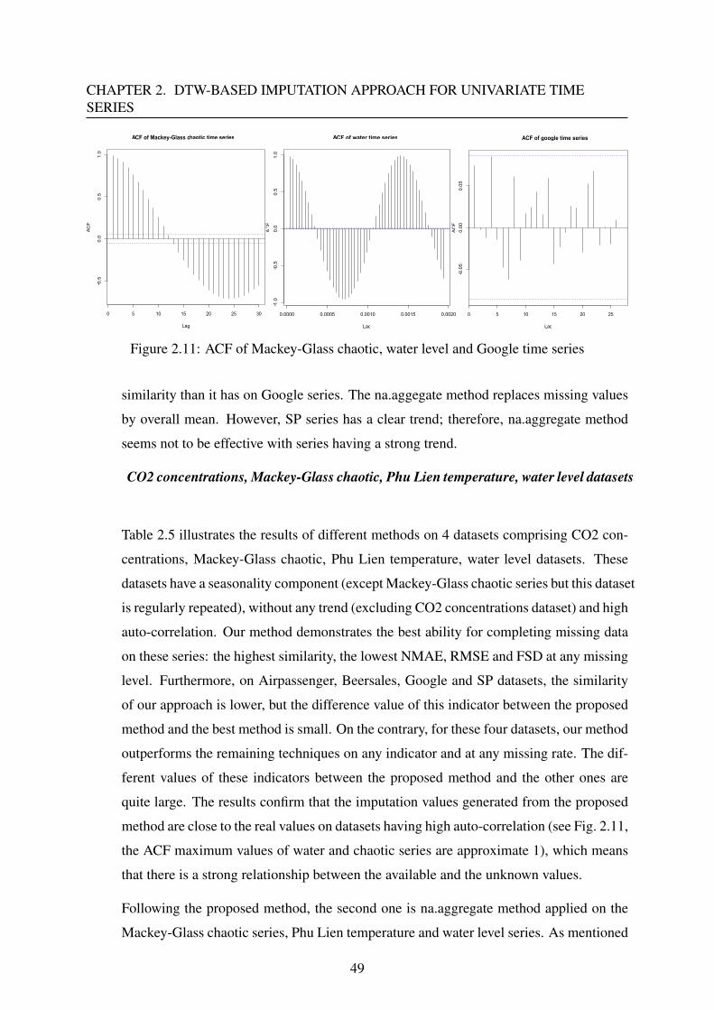
CHAPTER 2. DTW-BASED IMPUTATION APPROACH FOR UNIVARIATE TIMESERIES
0 5 10 15 20 25 30
−0.5
0.0
0.5
1.0
ACF of Mackey-Glass chaotic time series
Lag
ACF
0.0000 0.0005 0.0010 0.0015 0.0020
−1.0
−0.5
0.0
0.5
1.0
ACF of water time series
Lag
ACF
0 5 10 15 20 25
−0.05
0.00
0.05
ACF of google time series
Lag
ACF
Figure 2.11: ACF of Mackey-Glass chaotic, water level and Google time series
similarity than it has on Google series. The na.aggegate method replaces missing values
by overall mean. However, SP series has a clear trend; therefore, na.aggregate method
seems not to be effective with series having a strong trend.
CO2 concentrations, Mackey-Glass chaotic, Phu Lien temperature, water level datasets
Table 2.5 illustrates the results of different methods on 4 datasets comprising CO2 con-
centrations, Mackey-Glass chaotic, Phu Lien temperature, water level datasets. These
datasets have a seasonality component (except Mackey-Glass chaotic series but this dataset
is regularly repeated), without any trend (excluding CO2 concentrations dataset) and high
auto-correlation. Our method demonstrates the best ability for completing missing data
on these series: the highest similarity, the lowest NMAE, RMSE and FSD at any missing
level. Furthermore, on Airpassenger, Beersales, Google and SP datasets, the similarity
of our approach is lower, but the difference value of this indicator between the proposed
method and the best method is small. On the contrary, for these four datasets, our method
outperforms the remaining techniques on any indicator and at any missing rate. The dif-
ferent values of these indicators between the proposed method and the other ones are
quite large. The results confirm that the imputation values generated from the proposed
method are close to the real values on datasets having high auto-correlation (see Fig. 2.11,
the ACF maximum values of water and chaotic series are approximate 1), which means
that there is a strong relationship between the available and the unknown values.
Following the proposed method, the second one is na.aggregate method applied on the
Mackey-Glass chaotic series, Phu Lien temperature and water level series. As mentioned
49
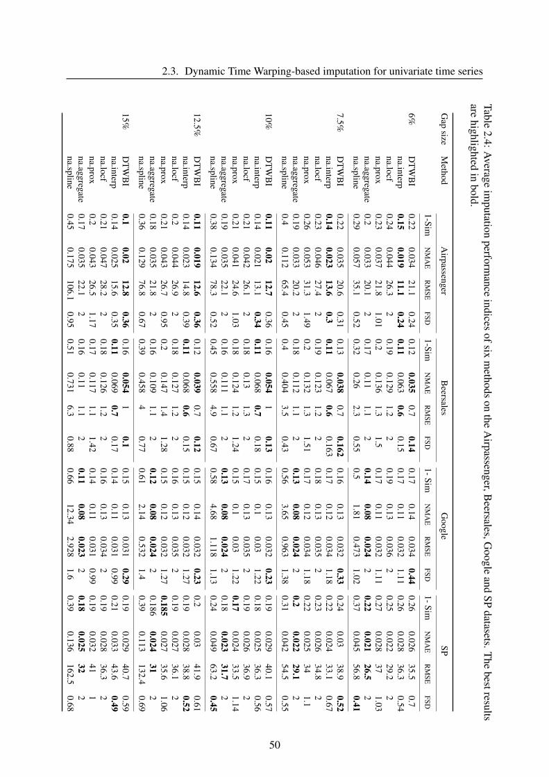
2.3. Dynamic Time Warping-based imputation for univariate time seriesTable
2.4:Average
imputation
performance
indicesofsix
methods
onthe
Airpassenger,B
eersales,Google
andSP
datasets.The
bestresultsare
highlightedin
bold.
Gap
sizeM
ethodA
irpassengerB
eersalesG
oogleSP
1-SimN
MA
ER
MSE
FSD1-Sim
NM
AE
RM
SEFSD
1-SimN
MA
ER
MSE
FSD1-Sim
NM
AE
RM
SEFSD
6%D
TW
BI
0.220.034
21.10.24
0.120.035
0.70.14
0.170.14
0.0340.44
0.260.026
35.50.7
na.interp0.15
0.01911.1
0.240.11
0.0630.6
0.150.17
0.110.032
1.110.26
0.02836.3
0.54na.locf
0.240.044
26.32
0.190.129
1.22
0.190.13
0.0362
0.250.022
29.22
na.prox0.23
0.03721.8
1.010.2
0.1361.3
1.50.17
0.110.032
1.110.27
0.02837
1.03na.aggregate
0.20.033
20.12
0.170.11
1.12
0.140.08
0.0242
0.220.021
26.52
na.spline0.29
0.05735.1
0.520.32
0.262.3
0.550.5
1.810.473
1.020.37
0.04556.8
0.41
7.5%D
TW
BI
0.220.035
20.60.31
0.130.038
0.70.162
0.160.13
0.0320.33
0.240.03
38.90.52
na.interp0.14
0.02313.6
0.30.11
0.0670.6
0.1630.17
0.120.034
1.180.22
0.02433.1
0.67na.locf
0.230.046
27.42
0.190.123
1.22
0.180.13
0.0352
0.230.026
34.82
na.prox0.26
0.05331.3
1.490.2
0.1321.3
1.510.17
0.120.034
1.180.22
0.02534
1.1na.aggregate
0.190.033
20.22
0.180.112
1.12
0.130.08
0.0242
0.20.022
29.12
na.spline0.4
0.11265.4
0.450.4
0.4043.5
0.430.56
3.650.963
1.380.31
0.04254.5
0.55
10%D
TW
BI
0.110.02
12.70.36
0.160.054
10.13
0.160.13
0.0320.23
0.190.029
40.10.57
na.interp0.14
0.02113.1
0.340.11
0.0680.7
0.180.15
0.10.03
1.220.18
0.02536.3
0.56na.locf
0.210.042
26.12
0.180.13
1.32
0.170.13
0.0352
0.190.026
36.92
na.prox0.21
0.04124.6
1.030.18
0.1241.2
1.240.15
0.10.03
1.220.17
0.02433.5
1.14na.aggregate
0.190.035
22.12
0.160.111
1.12
0.130.08
0.0242
0.180.023
31.72
na.spline0.38
0.13478.3
0.520.45
0.5584.9
0.670.58
4.681.118
1.130.24
0.04963.2
0.45
12.5%D
TW
BI
0.110.019
12.60.36
0.120.039
0.70.12
0.150.14
0.0320.23
0.20.03
41.90.61
na.interp0.14
0.02314.8
0.390.11
0.0680.6
0.150.15
0.120.032
1.270.19
0.02838.8
0.52na.locf
0.20.044
26.92
0.180.127
1.22
0.160.13
0.0352
0.190.027
36.12
na.prox0.21
0.04326.7
0.950.2
0.1471.4
1.280.15
0.120.032
1.270.185
0.02735.6
1.06na.aggregate
0.180.035
21.82
0.160.109
1.12
0.120.08
0.0242
0.1860.024
312
na.spline0.36
0.12976.8
0.670.39
0.4584
0.770.61
2.140.532
1.40.39
0.113132.4
0.69
15%D
TW
BI
0.10.02
12.80.36
0.160.054
10.1
0.150.13
0.0310.29
0.190.029
40.70.59
na.interp0.14
0.02515.6
0.350.11
0.0690.7
0.170.14
0.110.031
0.990.21
0.03343.6
0.49na.locf
0.210.047
28.22
0.180.126
1.22
0.160.13
0.0342
0.190.028
36.32
na.prox0.2
0.04326.5
1.170.17
0.1171.1
1.420.14
0.110.031
0.990.19
0.03241
1na.aggregate
0.170.035
22.12
0.160.11
1.12
0.110.08
0.0232
0.180.025
322
na.spline0.45
0.175106.1
0.950.51
0.7316.3
0.880.66
12.342.928
1.60.39
0.136162.5
0.68
50
CHAPTER 2. DTW-BASED IMPUTATION APPROACH FOR UNIVARIATE TIMESERIES
above (Table 2.3), these datasets have no trend, that is why na.aggregate could demon-
strate its ability. However, on the C02 series with clear trend, fully opposed to these 3
datasets, the performance of this method is the worst one.
Although na.interp method is well indicated for handling datasets with seasonality com-
ponent: here for these 4 datasets this approach does not illustrate its capability. It
gives the same results as na.approx method and lower results than our approach and
the na.aggregate one (on the Mackey-Glass chaotic, Phu Lien temperature and water se-
ries). For any dataset, na.spline method indicates the lowest performance. However on
the water series, this method has the least performance for completing missing values.
This means that the spline method is not suitable for this task.
In all datasets, FSD value of na.aggregate and na.locf methods always equals 2, because
they use the same value for all missing data (last value for na.locf method; overall mean
for na.aggregate).
Also, to be more persuasive about imputation results, we have conducted a new compar-
ison as follows: we randomly chose 10 windows having the same size of the gap, then
compute the average values to fill in the gap. Next we compare the results with all the
above methods using the same indicators as previously defined. Figure 2.12 illustrates
this comparison. Looking at figure 2.12, once again DTWBI demonstrates its ability ver-
sus the random selection of windows for complete missing values: the largest similarity,
the smallest RMSE and FSD.
• Comparison of visual performance
Tables 2.4, 2.5 indicate the quantitative comparison of 6 different methods for the task of
completing missing values. In this part, figures 2.13, 2.14, 2.15, 2.17, and 2.18 show the
comparison of visual imputation performance of different methods.
Fig. 2.13 presents the shape of imputation values of 5 existing methods (na.interp, na.locf,
na.approx, na.aggregate and na.spline) with the true values at position 106, the gap size
of 9 on the Airpassenger series. As we can notice on Table 2.4, considering low rates
of missing data, the proposed approach is less effective than na.interp and na.aggregate
methods for Airpassenger time series. However, when looking at Fig. 2.14, we find that
the shape of the imputation values generated from DTWBI method is very similar to
the shape of true values. Despite high similarity, low RMSE and NMAE, the shape of
imputation values yielded from na.aggregate method (Fig. 2.13) is not as good as the
51
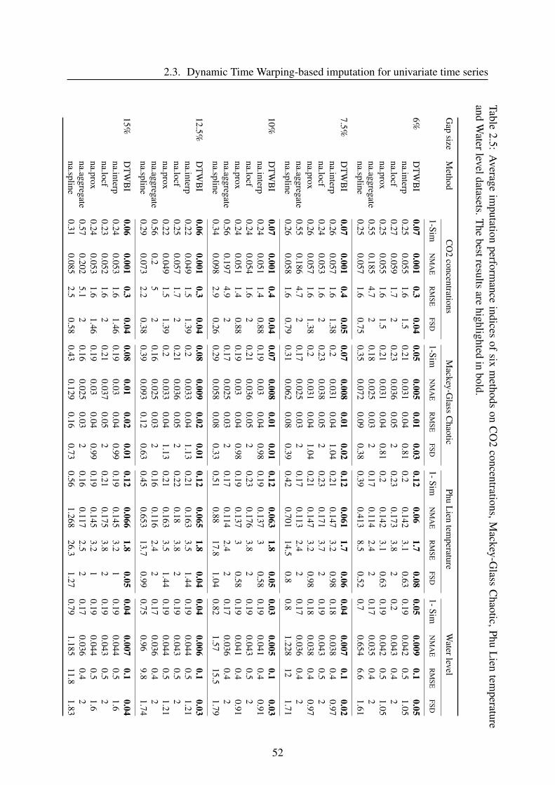
2.3. Dynamic Time Warping-based imputation for univariate time seriesTable
2.5:A
verageim
putationperform
anceindices
ofsix
methods
onC
O2
concentrations,Mackey-G
lassC
haotic,PhuL
ientem
peratureand
Waterleveldatasets.T
hebestresults
arehighlighted
inbold.
Gap
sizeM
ethodC
O2
concentrationsM
ackey-Glass
Chaotic
PhuL
ientem
peratureW
aterlevel
1-SimN
MA
ER
MSE
FSD1-Sim
NM
AE
RM
SEFSD
1-SimN
MA
ER
MSE
FSD1-Sim
NM
AE
RM
SEFSD
6%D
TW
BI
0.070.001
0.30.04
0.050.005
0.010.03
0.120.06
1.70.08
0.050.009
0.10.05
na.interp0.25
0.0551.6
1.50.21
0.0310.04
0.810.2
0.1423.1
0.630.19
0.0420.5
1.05na.locf
0.270.059
1.72
0.230.036
0.052
0.230.173
3.82
0.20.043
0.42
na.prox0.25
0.0551.6
1.50.21
0.0310.04
0.810.2
0.1423.1
0.630.19
0.0420.5
1.05na.aggregate
0.550.185
4.72
0.180.025
0.032
0.170.114
2.42
0.170.035
0.42
na.spline0.25
0.0571.6
0.750.35
0.0720.09
0.380.39
0.4138.5
0.520.7
0.6546.6
1.61
7.5%D
TW
BI
0.070.001
0.40.05
0.070.008
0.010.02
0.120.061
1.70.06
0.040.007
0.10.02
na.interp0.26
0.0571.6
1.380.2
0.0310.04
1.040.21
0.1473.2
0.980.18
0.0380.4
0.97na.locf
0.240.053
1.62
0.230.038
0.052
0.230.171
3.72
0.190.043
0.52
na.prox0.26
0.0571.6
1.380.2
0.0310.04
1.040.21
0.1473.2
0.980.18
0.0380.4
0.97na.aggregate
0.550.186
4.72
0.170.025
0.032
0.170.113
2.42
0.170.036
0.42
na.spline0.26
0.0581.6
0.790.31
0.0620.08
0.390.42
0.70114.5
0.80.8
1.22812
1.71
10%D
TW
BI
0.070.001
0.40.04
0.070.008
0.010.01
0.120.063
1.80.05
0.030.005
0.10.03
na.interp0.24
0.0511.4
0.880.19
0.030.04
0.980.19
0.1373
0.580.19
0.0410.4
0.91na.locf
0.240.054
1.62
0.210.036
0.052
0.230.176
3.82
0.190.043
0.52
na.prox0.24
0.0511.4
0.880.19
0.030.04
0.980.19
0.1373
0.580.19
0.0410.4
0.91na.aggregate
0.560.197
4.92
0.170.025
0.032
0.170.114
2.42
0.170.036
0.42
na.spline0.34
0.0982.9
0.260.29
0.0580.08
0.330.51
0.8817.8
1.040.82
1.5715.5
1.79
12.5%D
TW
BI
0.060.001
0.30.04
0.080.009
0.020.01
0.120.065
1.80.04
0.040.006
0.10.03
na.interp0.22
0.0491.5
1.390.2
0.0330.04
1.130.21
0.1633.5
1.440.19
0.0440.5
1.21na.locf
0.250.057
1.72
0.210.036
0.052
0.220.18
3.82
0.190.043
0.52
na.prox0.22
0.0491.5
1.390.2
0.0330.04
1.130.21
0.1633.5
1.440.19
0.0440.5
1.21na.aggregate
0.560.2
52
0.160.025
0.032
0.160.116
2.42
0.170.036
0.42
na.spline0.29
0.0732.2
0.380.39
0.0930.12
0.630.45
0.65313.7
0.990.75
0.969.8
1.74
15%D
TW
BI
0.060.001
0.30.04
0.080.01
0.020.01
0.120.066
1.80.05
0.040.007
0.10.04
na.interp0.24
0.0531.6
1.460.19
0.030.04
0.990.19
0.1453.2
10.19
0.0440.5
1.6na.locf
0.230.052
1.62
0.210.037
0.052
0.210.175
3.82
0.190.043
0.52
na.prox0.24
0.0531.6
1.460.19
0.030.04
0.990.19
0.1453.2
10.19
0.0440.5
1.6na.aggregate
0.570.202
5.12
0.160.025
0.032
0.160.117
2.52
0.170.036
0.42
na.spline0.31
0.0852.5
0.580.43
0.1290.16
0.730.56
1.26826.3
1.270.79
1.18511.8
1.83
52
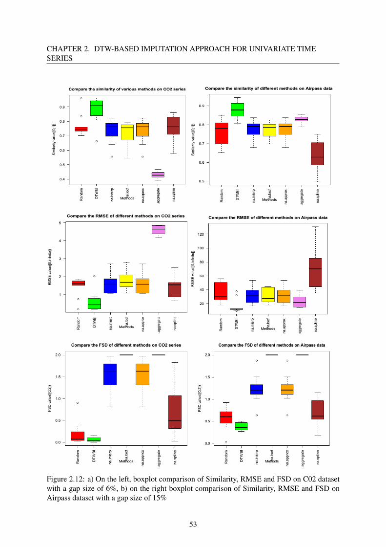
CHAPTER 2. DTW-BASED IMPUTATION APPROACH FOR UNIVARIATE TIMESERIES
Figure 2.12: a) On the left, boxplot comparison of Similarity, RMSE and FSD on C02 datasetwith a gap size of 6%, b) on the right boxplot comparison of Similarity, RMSE and FSD onAirpass dataset with a gap size of 15%
53
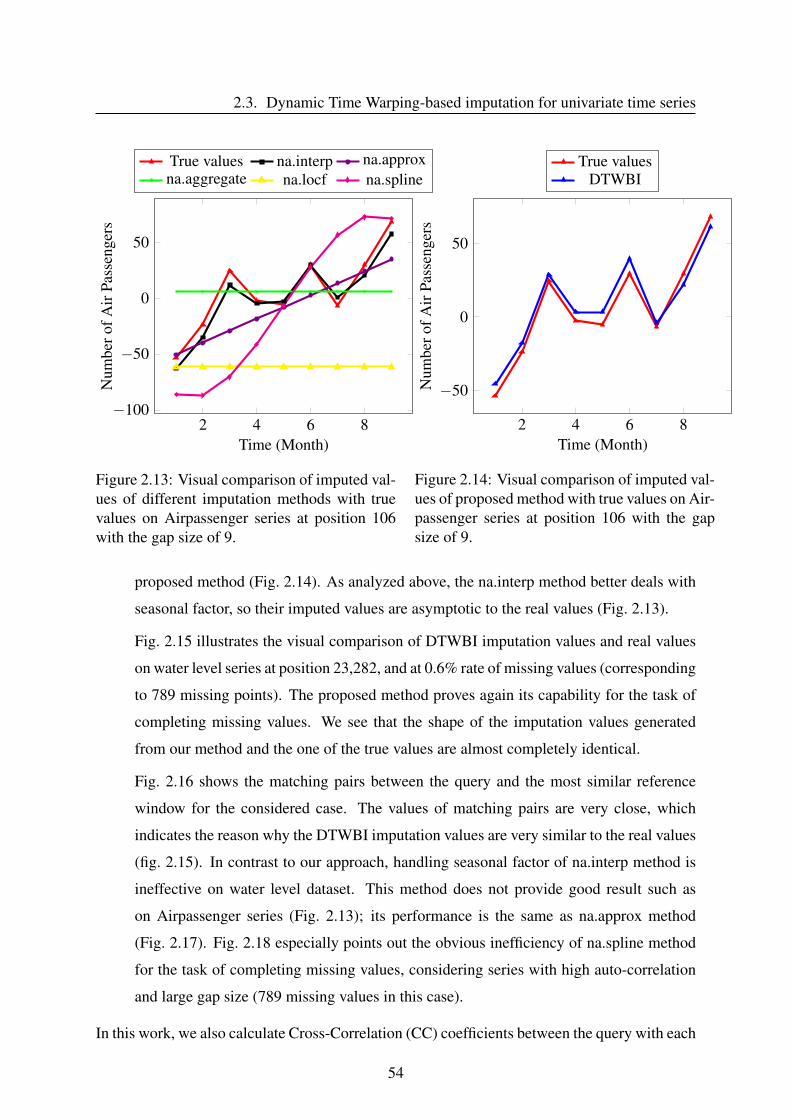
2.3. Dynamic Time Warping-based imputation for univariate time series
2 4 6 8−100
−50
0
50
Time (Month)
Num
bero
fAir
Pass
enge
rs
True values na.interp na.approxna.aggregate na.locf na.spline
Figure 2.13: Visual comparison of imputed val-ues of different imputation methods with truevalues on Airpassenger series at position 106with the gap size of 9.
2 4 6 8
−50
0
50
Time (Month)N
umbe
rofA
irPa
ssen
gers
True valuesDTWBI
Figure 2.14: Visual comparison of imputed val-ues of proposed method with true values on Air-passenger series at position 106 with the gapsize of 9.
proposed method (Fig. 2.14). As analyzed above, the na.interp method better deals with
seasonal factor, so their imputed values are asymptotic to the real values (Fig. 2.13).
Fig. 2.15 illustrates the visual comparison of DTWBI imputation values and real values
on water level series at position 23,282, and at 0.6% rate of missing values (corresponding
to 789 missing points). The proposed method proves again its capability for the task of
completing missing values. We see that the shape of the imputation values generated
from our method and the one of the true values are almost completely identical.
Fig. 2.16 shows the matching pairs between the query and the most similar reference
window for the considered case. The values of matching pairs are very close, which
indicates the reason why the DTWBI imputation values are very similar to the real values
(fig. 2.15). In contrast to our approach, handling seasonal factor of na.interp method is
ineffective on water level dataset. This method does not provide good result such as
on Airpassenger series (Fig. 2.13); its performance is the same as na.approx method
(Fig. 2.17). Fig. 2.18 especially points out the obvious inefficiency of na.spline method
for the task of completing missing values, considering series with high auto-correlation
and large gap size (789 missing values in this case).
In this work, we also calculate Cross-Correlation (CC) coefficients between the query with each
54
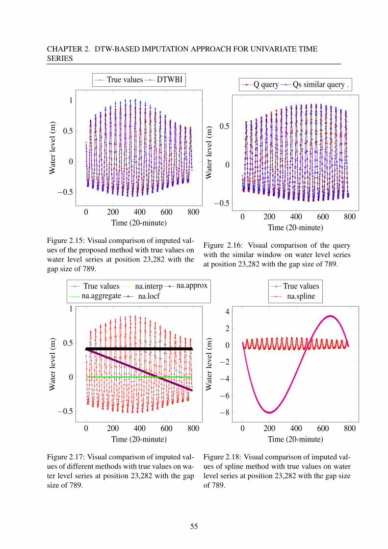
CHAPTER 2. DTW-BASED IMPUTATION APPROACH FOR UNIVARIATE TIMESERIES
0 200 400 600 800
−0.5
0
0.5
1
Time (20-minute)
Wat
erle
vel(
m)
True values DTWBI
Figure 2.15: Visual comparison of imputed val-ues of the proposed method with true values onwater level series at position 23,282 with thegap size of 789.
0 200 400 600 800
−0.5
0
0.5
Time (20-minute)
Wat
erle
vel(
m)
Q query Qs similar query .
Figure 2.16: Visual comparison of the querywith the similar window on water level seriesat position 23,282 with the gap size of 789.
0 200 400 600 800
−0.5
0
0.5
1
Time (20-minute)
Wat
erle
vel(
m)
True values na.interp na.approxna.aggregate na.locf
Figure 2.17: Visual comparison of imputed val-ues of different methods with true values on wa-ter level series at position 23,282 with the gapsize of 789.
0 200 400 600 800
−8
−6
−4
−2
0
2
4
Time (20-minute)
Wat
erle
vel(
m)
True valuesna.spline
Figure 2.18: Visual comparison of imputed val-ues of spline method with true values on waterlevel series at position 23,282 with the gap sizeof 789.
55
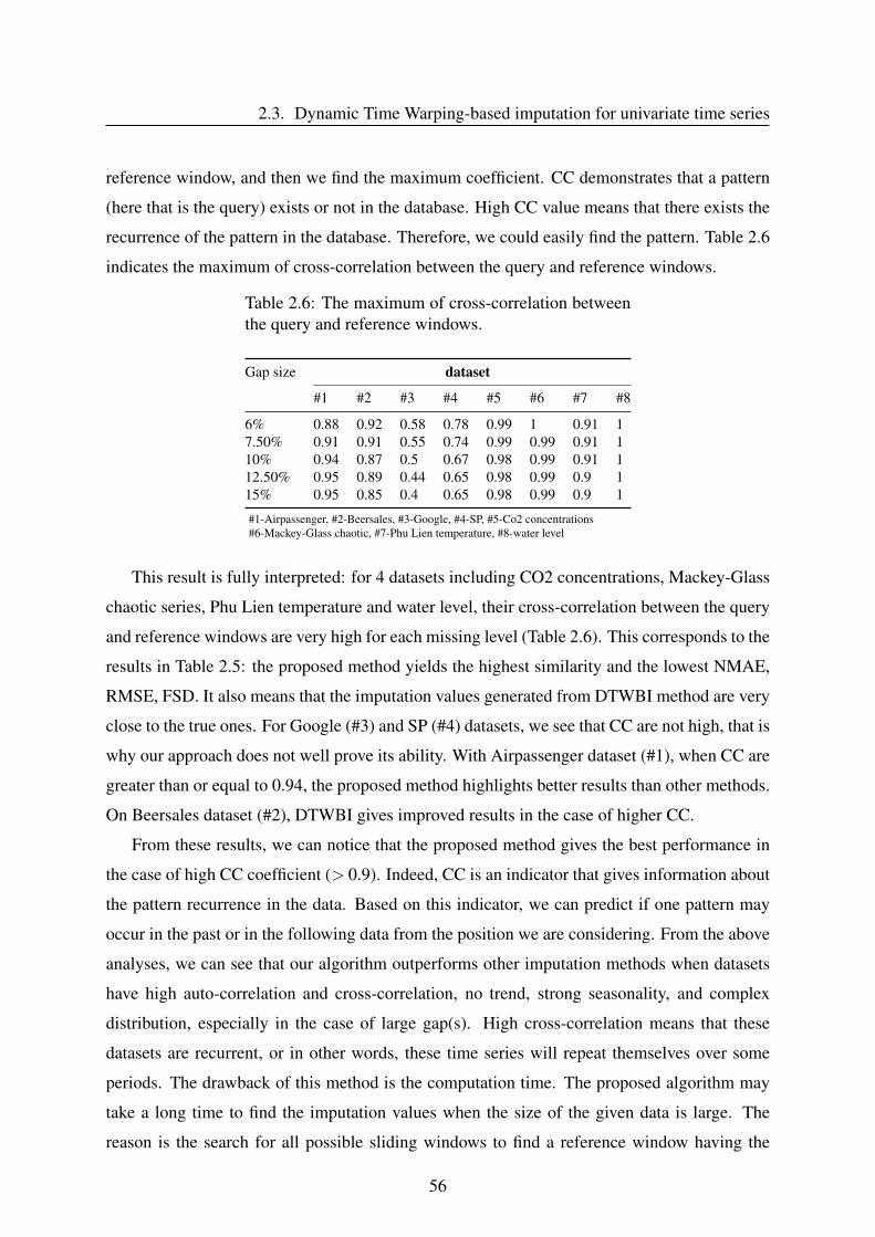
2.3. Dynamic Time Warping-based imputation for univariate time series
reference window, and then we find the maximum coefficient. CC demonstrates that a pattern
(here that is the query) exists or not in the database. High CC value means that there exists the
recurrence of the pattern in the database. Therefore, we could easily find the pattern. Table 2.6
indicates the maximum of cross-correlation between the query and reference windows.
Table 2.6: The maximum of cross-correlation betweenthe query and reference windows.
Gap size dataset
#1 #2 #3 #4 #5 #6 #7 #8
6% 0.88 0.92 0.58 0.78 0.99 1 0.91 17.50% 0.91 0.91 0.55 0.74 0.99 0.99 0.91 110% 0.94 0.87 0.5 0.67 0.98 0.99 0.91 112.50% 0.95 0.89 0.44 0.65 0.98 0.99 0.9 115% 0.95 0.85 0.4 0.65 0.98 0.99 0.9 1
#1-Airpassenger, #2-Beersales, #3-Google, #4-SP, #5-Co2 concentrations#6-Mackey-Glass chaotic, #7-Phu Lien temperature, #8-water level
This result is fully interpreted: for 4 datasets including CO2 concentrations, Mackey-Glass
chaotic series, Phu Lien temperature and water level, their cross-correlation between the query
and reference windows are very high for each missing level (Table 2.6). This corresponds to the
results in Table 2.5: the proposed method yields the highest similarity and the lowest NMAE,
RMSE, FSD. It also means that the imputation values generated from DTWBI method are very
close to the true ones. For Google (#3) and SP (#4) datasets, we see that CC are not high, that is
why our approach does not well prove its ability. With Airpassenger dataset (#1), when CC are
greater than or equal to 0.94, the proposed method highlights better results than other methods.
On Beersales dataset (#2), DTWBI gives improved results in the case of higher CC.
From these results, we can notice that the proposed method gives the best performance in
the case of high CC coefficient (> 0.9). Indeed, CC is an indicator that gives information about
the pattern recurrence in the data. Based on this indicator, we can predict if one pattern may
occur in the past or in the following data from the position we are considering. From the above
analyses, we can see that our algorithm outperforms other imputation methods when datasets
have high auto-correlation and cross-correlation, no trend, strong seasonality, and complex
distribution, especially in the case of large gap(s). High cross-correlation means that these
datasets are recurrent, or in other words, these time series will repeat themselves over some
periods. The drawback of this method is the computation time. The proposed algorithm may
take a long time to find the imputation values when the size of the given data is large. The
reason is the search for all possible sliding windows to find a reference window having the
56
CHAPTER 2. DTW-BASED IMPUTATION APPROACH FOR UNIVARIATE TIMESERIES
maximum similarity to the query.
2.3.4 Conclusion
In this study, we complete missing data on univariate time series based on the combination
of shape-feature extraction and DTW algorithms. The search of similar sequences by elastic
matching makes it possible to complete a database with missing values while respecting as
much as possible the dynamics and the shape of signals. Whereas applying the shape-feature
extraction algorithm allows to reduce the computing time of the proposed method.
The proposed imputation approach, namely DTWBI, for univariate time series data with
circular list permits to process a large dataset. DTWBI method has been tested on 8 datasets
with various size, ranging from small to very large database (Airpassenger, Beersales, Google,
SP, Co2 concentrations, Mackey-Glass chaotic, Phu Lien temperature, and water level). The ac-
curacy of imputation values yielded by DTWBI is compared with 5 existing methods (na.interp,
na.locf, na.approx, na.aggegate and na.spline) using 4 quantitative indicators (similarity, NMAE,
RMSE and FSD) applied to 5 different simulation missing levels. We also compare the visual
performance of these methods. The experiments show that our approach gives better results
than the other existing methods, and is the best robust method in the case of time series having
high cross-correlation and auto-correlation, large gap(s), complex distribution, and strong sea-
sonality. However, the proposed framework is restricted to applications where the necessary
assumption of recurring data in the time series is set up (high cross-correlation indicator), and
it requires computation time for very large missing intervals.
In the past decades, several studies investigated to improve classical DTW for better com-
paring the similarity between two curves by integrating the notions of slope (DDTW [48]) and
of curvature (AFBDTW [49]) or by changing the final DTW cost applied to classify [51] or
by comparing multidimensional series [50]. In order to assess the ability of different DTW
versions for filling in missing data, in the next section we perform a comparison of some DTW
variants (including DWT, DDTW, AFBDTW, DTW-D) applied to univariate time series impu-
tation.
57
2.4. Comparison of various DTW versions for completing missing values in univariate timeseries
2.4 Comparison of various DTW versions for completing
missing values in univariate time series
2.4.1 Introduction
In the previous section, we have proposed DTWBI method using classical DTW for recon-
structing database. And in the section 2.2 we have discussed several variants of DTW intro-
duced to improve the finding the similar of two sequences. In order to identify which variant is
more suitable for the imputation task, in this part, we carry out a comparison of the performance
of different DTW metrics applied to univariate time series imputation.
Dynamic Time Warping (DTW) [7] approach is used when no information are available,
the idea is to find a similar shape in a database to fill the missing values. Related works to
DTW are cited below, rare works deal with large gaps in univariate time series.
Hsu et al. [59] used k-Nearest Neighbors (k-NN) and DTW algorithms for completing
DNA data. They also performed comparing different versions of DTW algorithm for better
prediction and computation performance. Nevertheless, the authors did not mention to com-
plete long missing subsequences. In [60] a weighted k-NN version is combined with DTW to
compare multiple points in time simultaneously. DTW-cost is used as distance metric instead
of pointwise distance measurements. Kostadinova et al. [61] proposed an Integrative DTW-
Based Imputation algorithm that is particularly suited for the estimation of missing values in
gene expression time series data using multiple related information in datasets. This algorithm
identifies an appropriate set of estimation matrices by using DTW-cost distance in order to mea-
sure similarities between gene expression matrices. Yang et al. [62] also developed a method
to impute missing values in microarray time-series data based on the combination of k-NN and
DTW. In these three last cited works, the authors applied DTW method for completing missing
values in multivariate data. Imputation for consecutively missing values in univariate data is
not considered.
On the other hand, there is no application for surveying imputation algorithms with large
gap(s) size using directly DTW in the case of univariate time series. A gap is large when the
process could have significant changes during this missing period. In addition, recall that for
handing missing data within univariate time series, we must only rely on the available values
of this unique variable to estimate the incomplete values.
Therefore, the objective of this part is to build a framework for filling missing values in
58
CHAPTER 2. DTW-BASED IMPUTATION APPROACH FOR UNIVARIATE TIMESERIES
univariate time series and to perform a comparison of different similarity DTW metrics for the
imputation task. This allows to suggest the most suitable metric for the imputation of marine
univariate time series ensuring that results are reliable and high quality.
2.4.2 Imputation based on DTW metrics
We keep the same idea as DTWBI approach to perform completing missing data. That is, in
the previous section we have used the original DTW, this section we apply 3 different versions
of DTW for univariate time series imputation, namely, Derivative DTW (DDTW)[48], DTW-D
[51], and AFBDTW (Adaptive Feature Based DTW) [49]).
The approach consists in finding the most similar sub-sequence (Qs) to a query (Q), with
Q is the sub-sequence before a gap of T size at position t (Q = X [t − T : t − 1]). Then, we
complete this gap by the following sub-sequence of the Qs when this window is determined.
The mechanism is illustrated on the figure 2.9.
To obtain the Qs similar sub-sequence, we used different versions of DTW (as above men-
tioned). The dynamics and the shape of data before (resp. after) a gap are key-point of this
technique. The elastic matching is used to find similar window to the Q query of T size in the
search database. Once the most similar window is identified Qs, the following window Q f s
will be copied to the location of missing values.
2.4.3 Data presentation
Five datasets are used for evaluating the performance of different DTW versions, including:
Cua Ong temperature, Gas online, Chlorophyll-a, fluorescence, and water level. The last three
datasets are collected by IFREMER (France) in the eastern English Channel [3]. We have
chosen 4 new datasets and reused water level signal in order to focus on marine data which
were provided by the project we participate (CPER MARCO of our university (Chlorophyll-a,
fluorescence, water level) and Vietnam (Cua Ong temperature)). Another goal is also to test
our algorithm for different applications (so that we use Gas online series).
• Cua Ong temperature in oC - daily mean air temperature at the Cua Ong meteorological
station in Vietnam from 1/1/1973 to 31/12/1999.
• Gas online - weekly data on US finished motor gasoline products supplied (in thousands
of barrels per day) from 8/2/1991 to 4/11/2016 [63].
59
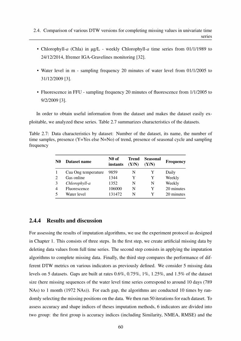
2.4. Comparison of various DTW versions for completing missing values in univariate timeseries
• Chlorophyll-a (Chla) in µg/L - weekly Chlorophyll-a time series from 01/1/1989 to
24/12/2014, Ifremer IGA-Gravelines monitoring [32].
• Water level in m - sampling frequency 20 minutes of water level from 01/1/2005 to
31/12/2009 [3].
• Fluorescence in FFU - sampling frequency 20 minutes of fluorescence from 1/1/2005 to
9/2/2009 [3].
In order to obtain useful information from the dataset and makes the dataset easily ex-
ploitable, we analyzed these series. Table 2.7 summarizes characteristics of the datasets.
Table 2.7: Data characteristics by dataset: Number of the dataset, its name, the number oftime samples, presence (Y=Yes else N=No) of trend, presence of seasonal cycle and samplingfrequency
N0 Dataset name N0 ofinstants
Trend(Y/N)
Seasonal(Y/N) Frequency
1 Cua Ong temperature 9859 N Y Daily2 Gas online 1344 Y Y Weekly3 Chlorophyll-a 1352 N N Weekly4 Fluorescence 106000 N Y 20 minutes5 Water level 131472 N Y 20 minutes
2.4.4 Results and discussion
For assessing the results of imputation algorithms, we use the experiment protocol as designed
in Chapter 1. This consists of three steps. In the first step, we create artificial missing data by
deleting data values from full time series. The second step consists in applying the imputation
algorithms to complete missing data. Finally, the third step compares the performance of dif-
ferent DTW metrics on various indicators as previously defined. We consider 5 missing data
levels on 5 datasets. Gaps are built at rates 0.6%, 0.75%, 1%, 1.25%, and 1.5% of the dataset
size (here missing sequences of the water level time series correspond to around 10 days (789
NAs) to 1 month (1972 NAs)). For each gap, the algorithms are conducted 10 times by ran-
domly selecting the missing positions on the data. We then run 50 iterations for each dataset. To
assess accuracy and shape indices of theses imputation methods, 6 indicators are divided into
two group: the first group is accuracy indices (including Similarity, NMEA, RMSE) and the
60
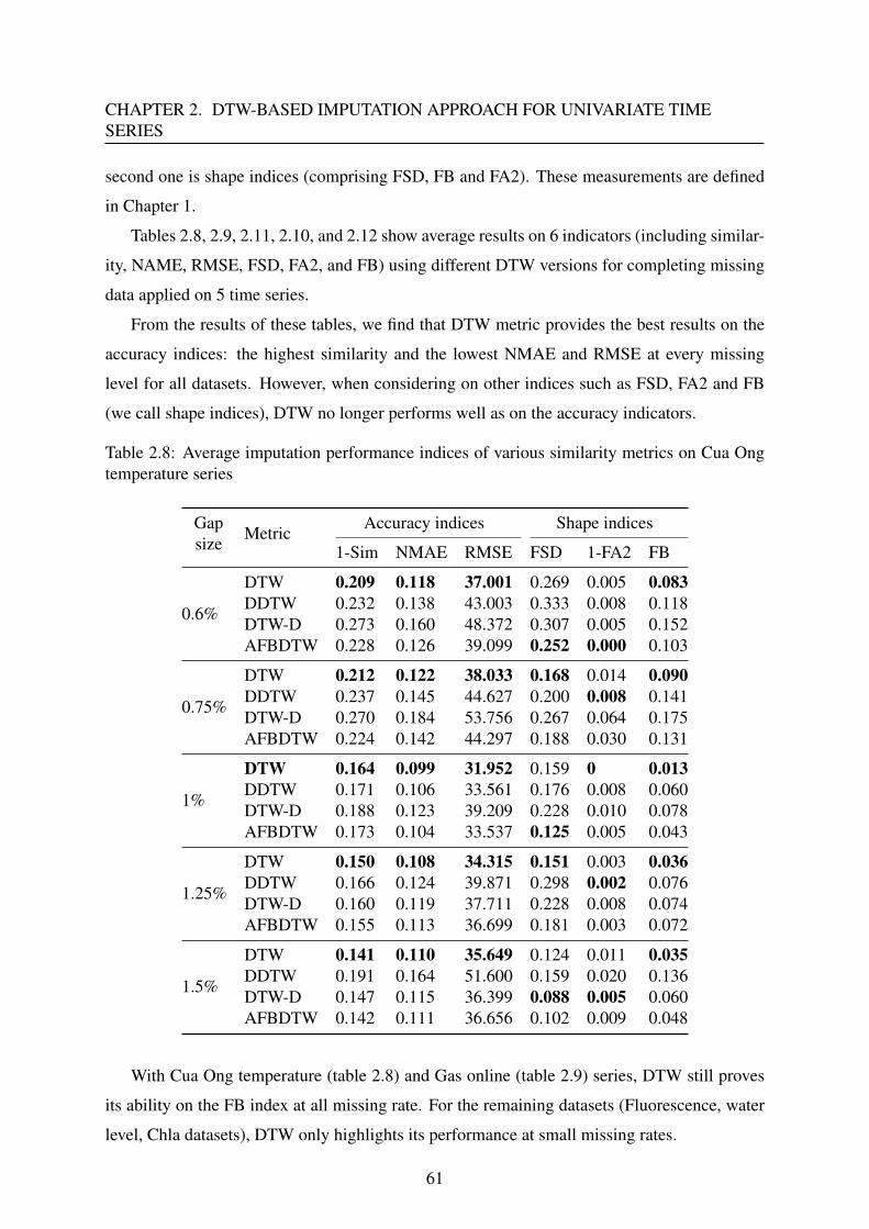
CHAPTER 2. DTW-BASED IMPUTATION APPROACH FOR UNIVARIATE TIMESERIES
second one is shape indices (comprising FSD, FB and FA2). These measurements are defined
in Chapter 1.
Tables 2.8, 2.9, 2.11, 2.10, and 2.12 show average results on 6 indicators (including similar-
ity, NAME, RMSE, FSD, FA2, and FB) using different DTW versions for completing missing
data applied on 5 time series.
From the results of these tables, we find that DTW metric provides the best results on the
accuracy indices: the highest similarity and the lowest NMAE and RMSE at every missing
level for all datasets. However, when considering on other indices such as FSD, FA2 and FB
(we call shape indices), DTW no longer performs well as on the accuracy indicators.
Table 2.8: Average imputation performance indices of various similarity metrics on Cua Ongtemperature series
Gapsize
MetricAccuracy indices Shape indices
1-Sim NMAE RMSE FSD 1-FA2 FB
0.6%
DTW 0.209 0.118 37.001 0.269 0.005 0.083DDTW 0.232 0.138 43.003 0.333 0.008 0.118DTW-D 0.273 0.160 48.372 0.307 0.005 0.152AFBDTW 0.228 0.126 39.099 0.252 0.000 0.103
0.75%
DTW 0.212 0.122 38.033 0.168 0.014 0.090DDTW 0.237 0.145 44.627 0.200 0.008 0.141DTW-D 0.270 0.184 53.756 0.267 0.064 0.175AFBDTW 0.224 0.142 44.297 0.188 0.030 0.131
1%
DTW 0.164 0.099 31.952 0.159 0 0.013DDTW 0.171 0.106 33.561 0.176 0.008 0.060DTW-D 0.188 0.123 39.209 0.228 0.010 0.078AFBDTW 0.173 0.104 33.537 0.125 0.005 0.043
1.25%
DTW 0.150 0.108 34.315 0.151 0.003 0.036DDTW 0.166 0.124 39.871 0.298 0.002 0.076DTW-D 0.160 0.119 37.711 0.228 0.008 0.074AFBDTW 0.155 0.113 36.699 0.181 0.003 0.072
1.5%
DTW 0.141 0.110 35.649 0.124 0.011 0.035DDTW 0.191 0.164 51.600 0.159 0.020 0.136DTW-D 0.147 0.115 36.399 0.088 0.005 0.060AFBDTW 0.142 0.111 36.656 0.102 0.009 0.048
With Cua Ong temperature (table 2.8) and Gas online (table 2.9) series, DTW still proves
its ability on the FB index at all missing rate. For the remaining datasets (Fluorescence, water
level, Chla datasets), DTW only highlights its performance at small missing rates.
61
2.4. Comparison of various DTW versions for completing missing values in univariate timeseries
Table 2.9: Average imputation performance indices of various similarity metrics on Gas onlineseries
Gapsize
MetricAccuracy indices Shape indices
1-Sim NMAE RMSE FSD 1-FA2 FB
0.6%
DTW 0.293 0.094 392.806 0.385 0 0.031DDTW 0.303 0.100 413.314 0.355 0 0.033DTW-D 0.336 0.113 457.966 0.438 0 0.031AFBDTW 0.453 0.237 894.008 0.460 0 0.094
0.75%
DTW 0.287 0.106 452.470 0.328 0 0.031DDTW 0.330 0.137 560.240 0.484 0 0.051DTW-D 0.330 0.131 533.966 0.440 0 0.047AFBDTW 0.455 0.237 891.465 0.351 0 0.095
1%
DTW 0.276 0.115 476.098 0.203 0 0.039DDTW 0.328 0.146 575.640 0.311 0 0.053DTW-D 0.315 0.131 545.698 0.174 0 0.046AFBDTW 0.384 0.227 859.176 0.304 0 0.084
1.25%
DTW 0.288 0.102 433.679 0.266 0 0.028DDTW 0.299 0.116 473.552 0.325 0 0.036DTW-D 0.313 0.118 482.555 0.241 0 0.036AFBDTW 0.300 0.113 457.787 0.341 0 0.037
1.5%
DTW 0.234 0.131 549.911 0.201 0 0.047DDTW 0.277 0.168 655.410 0.238 0 0.066DTW-D 0.266 0.149 598.538 0.121 0 0.048AFBDTW 0.346 0.216 820.442 0.280 0 0.084
According to Keogh et Pazzani [48], DDTW method presents better performance than the
original DTW by minimizing the number of duplicate points. However, the results in all the
tables show that DDTW is not suitable for handing the imputation task, it does not prove its
ability here.
AFBDTW was proposed in 2010 by Xie and Wiltgen [49]. This method takes into account
both the local and global features of the series for correspondences points instead of the value
itself or its derivative. That is the reason why AFBDTW proves the strength for the imputation
task at large missing rates, specially in large datasets.
DTW-D method is proposed for semi-supervisor classification. Therefore, when we applied
this method to complete missing values, DTW-D does not work well in all datasets at every
missing level. Nevertheless, when looking at FSD indicator in the table 2.9, DTW-D gives the
best results at large gaps (≥ 1%). The reason may be that Gas online series has both trend and
62
CHAPTER 2. DTW-BASED IMPUTATION APPROACH FOR UNIVARIATE TIMESERIES
Table 2.10: Average imputation performance indices of various similarity metrics on Fluores-cence series
Gapsize
MetricAccuracy indices Shape indices
1-Sim NMAE RMSE FSD 1-FA2 FB
0.6%
DTW 0.160 0.028 1.569 0.531 0.462 0.423DDTW 0.189 0.032 1.767 1.120 0.662 0.871DTW-D 0.327 0.067 3.732 0.950 0.740 1.060AFBDTW 0.198 0.035 1.991 0.853 0.545 0.685
0.75%
DTW 0.187 0.032 1.800 0.616 0.512 0.505DDTW 0.190 0.034 1.883 1.364 0.731 0.974DTW-D 0.378 0.101 5.272 1.175 0.802 1.219AFBDTW 0.212 0.036 2.068 0.654 0.576 0.724
1%
DTW 0.150 0.027 1.579 0.838 0.550 0.711DDTW 0.172 0.035 1.963 1.411 0.854 1.236DTW-D 0.295 0.070 3.749 1.122 0.778 1.141AFBDTW 0.157 0.027 1.606 0.782 0.606 0.800
1.25%
DTW 0.157 0.027 1.655 0.913 0.630 0.794DDTW 0.175 0.034 1.925 1.415 0.825 1.132DTW-D 0.362 0.104 5.740 1.218 0.834 1.302AFBDTW 0.160 0.030 1.756 0.778 0.629 0.744
1.50%
DTW 0.119 0.028 1.689 1.033 0.659 0.790DDTW 0.123 0.031 1.820 1.270 0.813 0.957DTW-D 0.259 0.083 4.690 1.042 0.811 1.145AFBDTW 0.142 0.038 2.319 0.791 0.622 0.656
seasonality component.
Besides, the shape of imputation values generated from methods using various DTW met-
rics (DTW, DDTW, DTW-D, AFBDTW) are also analyzed. Fig. 2.19 presents the form of
imputed values yielded by methods using different similarity metrics with the true values at po-
sition 444, the gap size of 14 (approximate 3 months of missing values) on the Chlorophyll-a.
DTW metric proves again its capability to deal with missing subsequence. The shape of the
imputation values generated from the method using DTW and the one of true values are very
close.
After the comparison of quantitative and visual performance of different DTW versions,
we carry out examining computational time of each metric. Table 2.13 shows that for large
datasets or large gaps, AFBDTW requires the longest computational time and DTW has at
least computing time.
63
2.4. Comparison of various DTW versions for completing missing values in univariate timeseries
Table 2.11: Average imputation performance indices of various similarity metrics on Chlaseries
MetricAccuracy indices Shape indices
1-Sim NMAE RMSE FSD 1-FA2 FB
DTW 0.308 0.069 4.609 0.597 0.413 0.381DDTW 0.339 0.091 5.707 0.692 0.463 0.476DTW-D 0.356 0.090 5.915 0.831 0.450 0.543AFBDTW 0.386 0.089 5.962 0.759 0.463 0.641
DTW 0.243 0.076 5.136 0.525 0.360 0.311DDTW 0.254 0.076 5.171 0.582 0.400 0.355DTW-D 0.303 0.094 6.481 0.897 0.480 0.492AFBDTW 0.281 0.086 5.876 0.646 0.460 0.535
DTW 0.185 0.071 4.990 0.444 0.393 0.394DDTW 0.205 0.088 6.207 0.501 0.443 0.468DTW-D 0.236 0.093 6.557 0.642 0.486 0.637AFBDTW 0.198 0.086 6.046 0.545 0.450 0.486
DTW 0.187 0.089 6.488 0.812 0.429 0.526DDTW 0.203 0.103 7.076 0.687 0.500 0.475DTW-D 0.216 0.105 7.352 0.775 0.518 0.409AFBDTW 0.222 0.104 7.136 0.686 0.512 0.404
DTW 0.205 0.090 6.226 0.435 0.545 0.408DDTW 0.216 0.097 6.772 0.407 0.515 0.460DTW-D 0.218 0.097 6.865 0.655 0.550 0.463AFBDTW 0.217 0.098 6.721 0.510 0.525 0.376
Also, we calculate Cross-Correlation (CC) coefficients between the query and each refer-
ence window and the maximum coefficient is extracted. CC demonstrates that a pattern (here
that is the query) exists or not in the database. High CC value means that there exists one or
more recurrence of the pattern in the database, that means: it is easy to find similar patterns. In
Table 2.14, we see that only for water level series, CC values are very high (approximate 1),
this explains why the similarity values are very high and the error index is very low.
2.4.5 Conclusion
This part compares a visual and quantitative performance of different DTW versions for uni-
variate time series imputation. The obtained results show that when considering the accuracy
of imputation values, DTW is the best robust and when regarding the shape of completed val-
64
CHAPTER 2. DTW-BASED IMPUTATION APPROACH FOR UNIVARIATE TIMESERIES
Table 2.12: Average imputation performance indices of various similarity metrics on waterlevel series
Gapsize
MetricAccuracy indices Shape indices
1-Sim NMAE RMSE FSD 1-FA2 FB
0.6%
DTW 0.042 0.037 0.401 0.045 0 0.019DDTW 0.042 0.037 0.402 0.045 0 0.022DTW-D 0.139 0.141 1.434 0.103 0.059 0.005AFBDTW 0.079 0.074 0.765 0.051 0.002 0.019
0.75%
DTW 0.037 0.033 0.355 0.017 0 0.009DDTW 0.042 0.038 0.401 0.019 0 0.010DTW-D 0.154 0.162 1.624 0.075 0.082 0.010AFBDTW 0.076 0.073 0.750 0.039 0.008 0.022
1%
DTW 0.033 0.030 0.333 0.026 0 0.012DDTW 0.034 0.030 0.333 0.027 0 0.014DTW-D 0.107 0.108 1.141 0.047 0.034 0.013AFBDTW 0.082 0.080 0.828 0.025 0.009 0.017
1.25%
DTW 0.039 0.035 0.373 0.025 0 0.009DDTW 0.039 0.035 0.373 0.025 0 0.009DTW-D 0.086 0.086 0.965 0.034 0.019 0.019AFBDTW 0.047 0.044 0.471 0.018 0.001 0.009
1.5%
DTW 0.045 0.042 0.442 0.030 0 0.022DDTW 0.045 0.043 0.450 0.032 0 0.025DTW-D 0.073 0.073 0.841 0.021 0.012 0.008AFBDTW 0.061 0.060 0.635 0.020 0.009 0.015
Table 2.13: Computational time of methods using different DTW metrics at missing rate 0.6%on various series in second (s)
MethodCua Ongtemperature
Gasonline Chla Fluorescence
Waterlevel
DTW 12.459 1.670 1.08 774.718 2081.388DDTW 13.112 1.700 1.07 786.543 2126.847DTW-D 12.543 1.671 1.10 761.831 2088.375AFBDTW 62.602 1.539 1.07 14219.51 49095.888
ues for the large gaps and datasets, AFBDTW is more suitable. This work highlights two
mains contributions. Firstly, we perform completing large missing subsequences in univariate
time series data. Secondly, we provide a quantitative and visual comparison of different DTW
algorithms applied to various datasets.
65
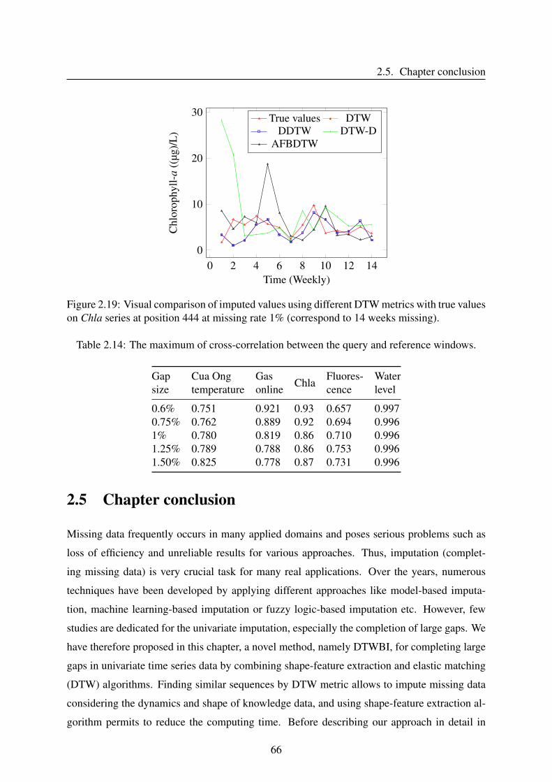
2.5. Chapter conclusion
0 2 4 6 8 10 12 140
10
20
30
Time (Weekly)
Chl
orop
hyll-
a((
µg)/
L)
True values DTWDDTW DTW-D
AFBDTW
Figure 2.19: Visual comparison of imputed values using different DTW metrics with true valueson Chla series at position 444 at missing rate 1% (correspond to 14 weeks missing).
Table 2.14: The maximum of cross-correlation between the query and reference windows.
Gapsize
Cua Ongtemperature
Gasonline Chla
Fluores-cence
Waterlevel
0.6% 0.751 0.921 0.93 0.657 0.9970.75% 0.762 0.889 0.92 0.694 0.9961% 0.780 0.819 0.86 0.710 0.9961.25% 0.789 0.788 0.86 0.753 0.9961.50% 0.825 0.778 0.87 0.731 0.996
2.5 Chapter conclusion
Missing data frequently occurs in many applied domains and poses serious problems such as
loss of efficiency and unreliable results for various approaches. Thus, imputation (complet-
ing missing data) is very crucial task for many real applications. Over the years, numerous
techniques have been developed by applying different approaches like model-based imputa-
tion, machine learning-based imputation or fuzzy logic-based imputation etc. However, few
studies are dedicated for the univariate imputation, especially the completion of large gaps. We
have therefore proposed in this chapter, a novel method, namely DTWBI, for completing large
gaps in univariate time series data by combining shape-feature extraction and elastic matching
(DTW) algorithms. Finding similar sequences by DTW metric allows to impute missing data
considering the dynamics and shape of knowledge data, and using shape-feature extraction al-
gorithm permits to reduce the computing time. Before describing our approach in detail in
66
CHAPTER 2. DTW-BASED IMPUTATION APPROACH FOR UNIVARIATE TIMESERIES
Section 2.3.1, we present the basic of DTW and its variants in the first part of this chapter. In
the last section, we perform a comparison of different versions of DTW in order to determine
a more customized method for the imputation of marine univariate time series ensuring that
results are reliable and high quality. From the results, we can conclude that when considering
the accuracy of imputation values, DTW is the best robust and when regarding the shape of
completed values for the large gaps and datasets, AFBDTW is more suitable.
List of Publications and valuations related to this chapter
1. Thi-Thu-Hong Phan, Emilie Poisson Caillault, Alain Lefebvre, André Bigand, "Dy-
namic Time Warping-based imputation for univariate time series data", Pattern Recog-
nition Letters. Available online 16 August 2017. In Press, Accepted Manuscript. DOI:
10.1016/j.patrec.2017.08.019.
2. Emilie Poisson Caillault, Kelly Grassi, Thi Thu Hong Phan, Camille Dezecache, Jean
Prygiel, Alain Lefebvre, "DTWBI & uHMM R-packages for multivariate time series pre-
processing and interpretation", 26th Earth Science Meeting, 22-26 October 2018, Lille,
France.
3. Thi-Thu-Hong Phan, Emilie Poisson Caillault, Alain Lefebvre, André Bigand, "Which
DTW Method Applied to Marine Univariate Time Series Imputation", OCEANS 2017
MTS/IEEE, Aberdeen, Scotland, 06/2017. DOI: 10.1109/OCEANSE.2017.8084598.
4. Caillault-Poisson E., Lefebvre A., Hébert P.A., Phan, T.T.H., Ternynck P., Marson Q.,
Rizik A., Wacquet G., Artigas F., Bigand A, "Méthodologie(s) du traitement du sig-
nal à la classification/modélisation pour la compréhension de la dynamique des efflo-
rescences phytoplanctoniques", Journée du CPER MARCO, 26 juin 2017, Boulogne sur
Mer, France.
5. Caillault-Poisson E., Phan, T.T.H., Rizik A., Ternynck P., Bigand A, Lefebvre A, "New
developments to fill the gap in high frequency data series and to integrate knowledge in
Markov modeling of phytoplankton dynamics", EEC’2017: The Eastern English Channel
Conference, Wimereux, 06/06/2017, France.
6. Thi-Thu-Hong Phan, Emilie Poisson Caillault, Alain Lefebvre, André Bigand. Which
67
2.5. Chapter conclusion
DTW Method Applied to Marine Univariate Time Series Imputation, GRAISyHM: Sémi-
naire des doctorants en traitement du signal et/ou de l’image, 26/04/2017, Lille, France.
7. Thi-Thu-Hong Phan, Emilie Poisson Caillault, Alain Lefebvre, André Bigand. Which
DTW Method Applied to Marine Univariate Time Series Imputation, Journée Scien-
tifique du Conseil Scientifique du GIS Campus de la Mer, 03/04/2017, Boulogne sur
Mer, France.
8. R-Package
DWTBI R-package https://cran.r-project.org/web/packages/DTWBI/index.html
68
Chapter 3Imputation approaches for uncorrelated
multivariate time series
Contents3.1 Introduction . . . . . . . . . . . . . . . . . . . . . . . . . . . . . . . . . . 69
3.2 Dynamic Time Warping-based uncorrelated multivariate time series im-putation . . . . . . . . . . . . . . . . . . . . . . . . . . . . . . . . . . . . 73
3.2.1 DTWUMI - Proposed approach . . . . . . . . . . . . . . . . . . . . 73
3.2.2 Validation procedure . . . . . . . . . . . . . . . . . . . . . . . . . . 75
3.2.3 Results and discussion . . . . . . . . . . . . . . . . . . . . . . . . . 79
3.2.4 Conclusion . . . . . . . . . . . . . . . . . . . . . . . . . . . . . . . 84
3.3 Proposed method based on an hybrid similarity measure . . . . . . . . . 85
3.3.1 Methods based on fuzzy similarity measure . . . . . . . . . . . . . . 85
3.3.2 FSMUMI-Proposed approach . . . . . . . . . . . . . . . . . . . . . 87
3.3.3 Validation procedure . . . . . . . . . . . . . . . . . . . . . . . . . . 93
3.3.4 Results and discussion . . . . . . . . . . . . . . . . . . . . . . . . . 96
3.3.5 Conclusion . . . . . . . . . . . . . . . . . . . . . . . . . . . . . . . 107
3.4 Chapter conclusion . . . . . . . . . . . . . . . . . . . . . . . . . . . . . . 107
3.1 Introduction
In the previous chapter we presented our proposal to fill missing data in univariate time series
based on the combination of shape-feature extraction and DTW methods. The proposed ap-
69
3.1. Introduction
proach exploits observed data on the univariate time series to estimate the missing values. In
this chapter, we investigate to fill large incomplete data in low/un-correlated multivariate time
series by taking advantage the property of uncorrelated multivariate data.
In the literature, many successful studies have been devoted to multivariate time series
imputation such as [64, 65, 66, 67, 68, 69, 70, 71, 72, 73, 74, 75, 60]. Imputation techniques can
be categorized in different perspectives: model-based, machine learning-based and clustering-
based imputation techniques.
In view of the model-based imputation, two main methods were proposed. The first method
was introduced by Schafer [64]. With the hypothesis that all variables follow a multivariate nor-
mal distribution, this approach is based on the multivariate normal (MVN) model to determine
completion values. And, the second method, namely MICE, was developed by van Buuren et
al. [65] and Raghunathan et al. [66]. This method uses chained equations to fill in incomplete
data: for each variable with missing values, MICE computes the imputation data by exploiting
the relations between all other variables.
According to the concept of machine learning-based imputation, many studies focus on
completion of missing data in multivariate time series. Stekhoven and Bühlmann [76] im-
plemented missForest based on the Random Forest (RF) method for multivariate imputation.
P.Bonissone et al. [77] proposed a fuzzy version of RF that they named fuzzy random for-
est FRF. At the moment FRF is only devoted to classification and in our case FRF may be
only interesting to separate correlated and un-correlated variables in multivariate time series
if necessary. In [71], Shah et al. investigated a variant of MICE which fills in each variable
using the estimation generated from RF. The results showed that the combination of MICE and
RF was more efficient than original methods for multivariate imputation. K-Nearest Neigh-
bors (k-NN)-based imputation is also a popular method for completing missing values such as
[72, 78, 59, 62, 61, 60]. This approach identifies the k most similar patterns in the space of
available features to impute missing data.
Besides these principal techniques, clustering-based imputation approaches are considered
as power tools for completing missing values thanks to their ability to detect similar patterns.
The objective of these techniques is to separate the data into several clusters when satisfying
the following conditions: maximizing the intercluster similarity and minimizing intracluster
dissimilarity. Li et al. [79] proposed the k-means clustering imputation technique that estimates
missing values using the final cluster information. The fuzzy c-means (FcM) clustering is a
common extension of k-means. The squared-norm is applied to measure the similarity between
70
CHAPTER 3. IMPUTATION APPROACHES FOR UNCORRELATED MULTIVARIATETIME SERIES
cluster centers and data points. Different applications based on FcM are investigated for the
imputation task as [80, 81, 82, 83, 84, 85, 86, 87]. Wang et al. [88] used FcM based on DTW
to successfully forecast long-term time series.
In general, most of the imputation algorithms for multivariate time series take advantage of
dependencies between attributes to predict missing values. The correlations make it possible
to estimate missing data using the available values of the other variables. However, it is not
efficient for multivariate series having low-or un-correlated features (case of MAREL Carnot
dataset). For handling missing values or intervals in this case, we must only rely on the observed
values of the unique variable containing missing data to predict the incomplete values. Besides,
completion of missing values for this type of data has received little attention in the literature
when comparing with the imputation of correlated multivariate time series.
One way to solve the problem of missing values in this case is to find the same behavior
or shape. This is equivalent to retrieve similar values. In the literature, similarity measures are
used for broad range of applications such as classification, anomaly detection [89], retrieval
system [15], recommendation systems [17], imputation [90] and pattern recognition [20]. So,
our idea to deal with large gaps in low/un-correlated multivariate time series, is to retrieve
similar sub-sequences on unique signal having missing values by using a similarity measure.
Moreover, weighting of different similarity measures could provide better prediction accu-
racy in many applications such as [15, 17, 18, 19]. Particularly, imperfect time series can be
modelled using fuzzy sets introduced by Zadeh [91, 92]. The fuzzy approach makes it possible
to deal with imprecise and uncertain circumstances [15]. The successfully use of fuzzy-based
similarity measure [20, 15, 17] and weighting of different similarity measures [17, 18, 19] leads
us to study the ability of fuzzy-weighted similarity measure to complete missing values in un-
correlated multivariate time series. To develop a new fuzzy-weighted similarity measure, in
this study, we use a rule-based technique. This technique is power and widely employed in
different studies like [15, 21, 22, 23, 24].
According to our knowledge, there is no application devoted to complete large gap(s) in
uncorrelated multivariate time series using a fuzzy-weighted similarity measure and directly
using DTW cost as a similarity criterion. Therefore, in this chapter, we propose two new
approaches for filling large missing values in low/un-correlated multivariate time series by
exploiting features of the uncorrelated data as follows:
1. DTWUMI method
71
3.1. Introduction
• We extend our previous method (DTWBI) to impute large missing values in uncor-
related multivariate time series, namely DTWUMI.
• We just consider one query and this query is built by taking into account all the
signals either before or after each gap (i.e. preserving the time index for all the
variables). The last allows to assure an acceptable similarity for each signal within
the time series in the same temporal window.
• We only find the most similar window to the query and only utilize DTW cost as
the similarity criterion to retrieve similar windows.
• We directly use data from the window following or preceding of the most similar
window on the signal containing the considered gap to fill in the missing values.
2. FSMUMI method
• Since time series data are multidimensional but they are uncorrelated (or low-
correlated), so we take advantage of this feature to handle each signal one by one.
This is explained in step of building queries: on each incomplete signal, for each
gap, we build two queries, one query before the gap and one query after this gap.
• We take into account an uncertainty factor. So, we develop a new fuzzy-weighted
similarity measure by weighting of different popular similarity distances based on
fuzzy logic. To obtain this similarity measure we propose to use a new fuzzy-rule
interpolation scheme that adapts to the fuzzy rule-based structure and adapts to the
finding of missing patterns in time series.
• We retrieve the two most similar windows with two queries on the data before the
gap and data after the gap (this means that we process two separated databases) on
the signal containing the gap using the new similarity measure.
• The final imputation values are the average of 2 vectors following and preceding of
the two most similar windows.
And then we will compare both methods with published algorithms
Moreover, estimating the distribution of missing values and whole signals is very difficult,
so our approaches make an assumption of effective patterns (or recurrent data, here a pattern
corresponds to the sub-sequence before (resp. after) a gap) on each signal.
72
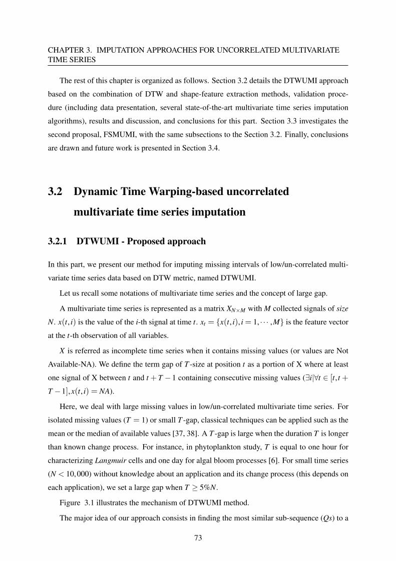
CHAPTER 3. IMPUTATION APPROACHES FOR UNCORRELATED MULTIVARIATETIME SERIES
The rest of this chapter is organized as follows. Section 3.2 details the DTWUMI approach
based on the combination of DTW and shape-feature extraction methods, validation proce-
dure (including data presentation, several state-of-the-art multivariate time series imputation
algorithms), results and discussion, and conclusions for this part. Section 3.3 investigates the
second proposal, FSMUMI, with the same subsections to the Section 3.2. Finally, conclusions
are drawn and future work is presented in Section 3.4.
3.2 Dynamic Time Warping-based uncorrelated
multivariate time series imputation
3.2.1 DTWUMI - Proposed approach
In this part, we present our method for imputing missing intervals of low/un-correlated multi-
variate time series data based on DTW metric, named DTWUMI.
Let us recall some notations of multivariate time series and the concept of large gap.
A multivariate time series is represented as a matrix XN×M with M collected signals of size
N. x(t, i) is the value of the i-th signal at time t. xt = {x(t, i), i = 1, · · · ,M} is the feature vector
at the t-th observation of all variables.
X is referred as incomplete time series when it contains missing values (or values are Not
Available-NA). We define the term gap of T -size at position t as a portion of X where at least
one signal of X between t and t +T −1 containing consecutive missing values (∃i|∀t ∈ [t, t +
T −1],x(t, i) = NA).
Here, we deal with large missing values in low/un-correlated multivariate time series. For
isolated missing values (T = 1) or small T -gap, classical techniques can be applied such as the
mean or the median of available values [37, 38]. A T -gap is large when the duration T is longer
than known change process. For instance, in phytoplankton study, T is equal to one hour for
characterizing Langmuir cells and one day for algal bloom processes [6]. For small time series
(N < 10,000) without knowledge about an application and its change process (this depends on
each application), we set a large gap when T ≥ 5%N.
Figure 3.1 illustrates the mechanism of DTWUMI method.
The major idea of our approach consists in finding the most similar sub-sequence (Qs) to a
73
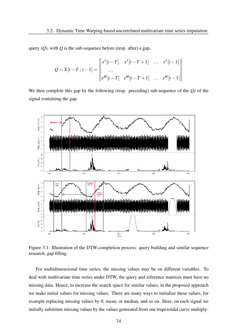
3.2. Dynamic Time Warping-based uncorrelated multivariate time series imputation
query (Q), with Q is the sub-sequence before (resp. after) a gap,
Q = X [t−T : t−1] =
∥∥∥∥∥∥∥∥x1[t−T ] x1[t−T + 1] . . . x1[t−1]
. . .
xM[t−T ] xM[t−T + 1] . . . xM[t−1]
∥∥∥∥∥∥∥∥We then complete this gap by the following (resp. preceding) sub-sequence of the Qs of the
signal containing the gap.
Figure 3.1: Illustration of the DTW-completion process: query building and similar sequenceresearch, gap filling.
For multidimensional time series, the missing values may be on different variables. To
deal with multivariate time series under DTW, the query and reference matrices must have no
missing data. Hence, to increase the search space for similar values, in the proposed approach
we make initial values for missing values. There are many ways to initialize these values, for
example replacing missing values by 0, mean, or median, and so on. Here, on each signal we
initially substitute missing values by the values generated from one trapezoidal curve multiply-
74
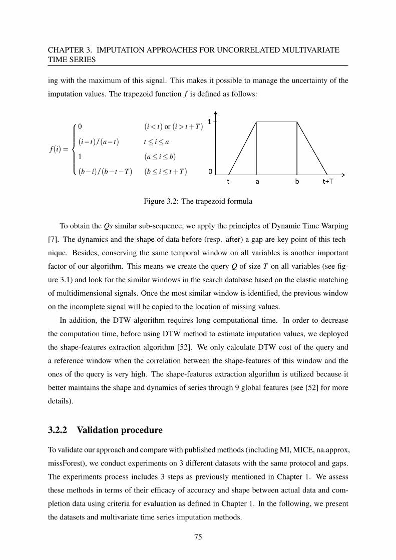
CHAPTER 3. IMPUTATION APPROACHES FOR UNCORRELATED MULTIVARIATETIME SERIES
ing with the maximum of this signal. This makes it possible to manage the uncertainty of the
imputation values. The trapezoid function f is defined as follows:
Figure 3.2: The trapezoid formula
To obtain the Qs similar sub-sequence, we apply the principles of Dynamic Time Warping
[7]. The dynamics and the shape of data before (resp. after) a gap are key point of this tech-
nique. Besides, conserving the same temporal window on all variables is another important
factor of our algorithm. This means we create the query Q of size T on all variables (see fig-
ure 3.1) and look for the similar windows in the search database based on the elastic matching
of multidimensional signals. Once the most similar window is identified, the previous window
on the incomplete signal will be copied to the location of missing values.
In addition, the DTW algorithm requires long computational time. In order to decrease
the computation time, before using DTW method to estimate imputation values, we deployed
the shape-features extraction algorithm [52]. We only calculate DTW cost of the query and
a reference window when the correlation between the shape-features of this window and the
ones of the query is very high. The shape-features extraction algorithm is utilized because it
better maintains the shape and dynamics of series through 9 global features (see [52] for more
details).
3.2.2 Validation procedure
To validate our approach and compare with published methods (including MI, MICE, na.approx,
missForest), we conduct experiments on 3 different datasets with the same protocol and gaps.
The experiments process includes 3 steps as previously mentioned in Chapter 1. We assess
these methods in terms of their efficacy of accuracy and shape between actual data and com-
pletion data using criteria for evaluation as defined in Chapter 1. In the following, we present
the datasets and multivariate time series imputation methods.
75
3.2. Dynamic Time Warping-based uncorrelated multivariate time series imputation
3.2.2.1 Data presentation
Three multivariate time series are handled in this study. We choose one from KEEL reposi-
tory, one simulated dataset (this permits to control the criterion of correlations and the amount
of missing data) and one real dataset hourly collected by IFREMER (France) in the eastern
English Channel.
NNGC1_F1_V1_003 (NNGC) dataset [93]: This time series contains transportation data
(4 attributes and 1,745 instants) including highway traffic, traffic data of cars in tunnels, traffic
at automatic payment systems on highways, traffic of individuals on subway systems, domestic
aircraft flights, shipping imports, border crossings, pipeline flows and rail transportation. The
data contains a time series of hourly frequency.
Simulated dataset: In the second experiment, a simulated dataset including 3 signals is
produced in the following: For the first variable, we use 5 sine functions that have different
frequencies and amplitudes F = { f1, f2, f3, f4, f5}. Next, 3 various noise levels are added to
data F , S = {F ,F + noise1,F + noise2,F + noise3}. We then repeat S 4 times (this dataset
has 32,000 sampled points). In this study, we treat with missing data in low/un-correlated
multivariate time series. So to satisfy this condition, the two remaining signals are generated
based on the first signal with the correlations between these signals are low (≤ 0.1%). We apply
the Corgen function of ecodist R-package [94] to create the second and the third variables.
MAREL-Carnot dataset [3]: The third experiment is conducted on MAREL-Carnot dataset.
This dataset consists of nineteen series such as phosphate, salinity, turbidity, water temperature,
fluorescence, water level,... that characterize seawater. These signals were collected from the
1st January 2005 to the 9th February 2009 at 20 minutes frequency. Here they were hourly sam-
pled, so they have 35,334 time samples. But the data include many missing values, the size of
missing data varies on each signal. For assessing the performance of the proposed method and
comparing with other approaches, we chose a subgroup including fluorescence, water level,
and water temperature (the water level and the fluorescence signals are complete data, while
water temperature contains isolated missing values and gaps). We select these signals because
their correlations are low.
After completing missing values, completion data will be compared with actual values in
the full series to evaluate the ability of different imputation methods. Therefore, it is necessary
to fill missing values in the water temperature. To ensure the fairness of all algorithms, filling
in the water temperature series is performed by na.interp method ([53]).
76
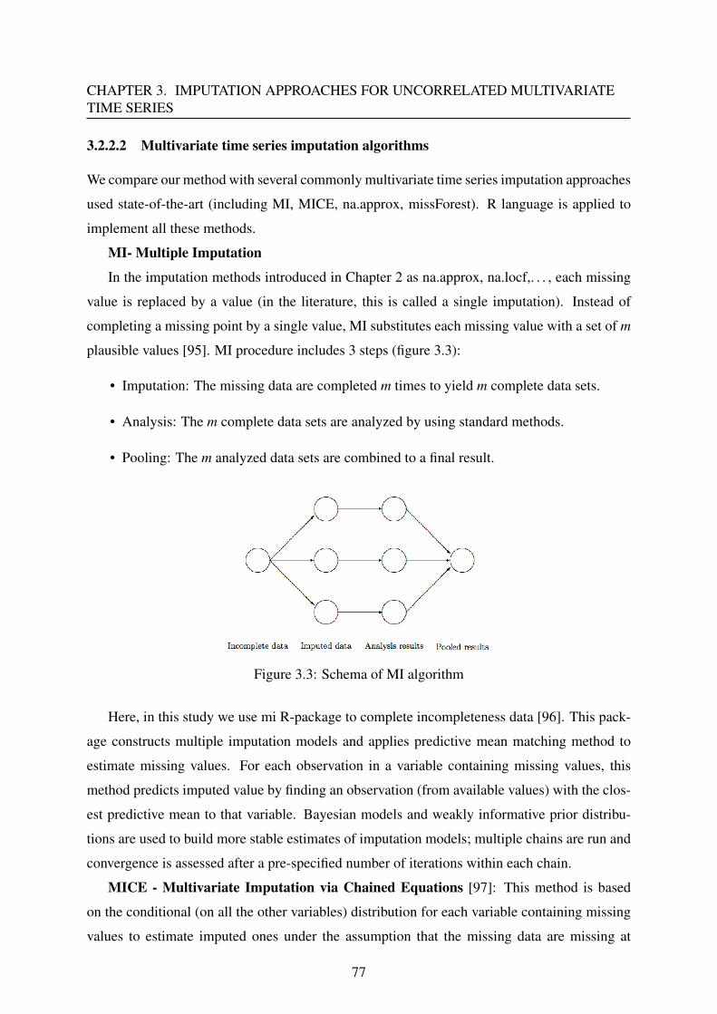
CHAPTER 3. IMPUTATION APPROACHES FOR UNCORRELATED MULTIVARIATETIME SERIES
3.2.2.2 Multivariate time series imputation algorithms
We compare our method with several commonly multivariate time series imputation approaches
used state-of-the-art (including MI, MICE, na.approx, missForest). R language is applied to
implement all these methods.
MI- Multiple Imputation
In the imputation methods introduced in Chapter 2 as na.approx, na.locf,. . . , each missing
value is replaced by a value (in the literature, this is called a single imputation). Instead of
completing a missing point by a single value, MI substitutes each missing value with a set of m
plausible values [95]. MI procedure includes 3 steps (figure 3.3):
• Imputation: The missing data are completed m times to yield m complete data sets.
• Analysis: The m complete data sets are analyzed by using standard methods.
• Pooling: The m analyzed data sets are combined to a final result.
Figure 3.3: Schema of MI algorithm
Here, in this study we use mi R-package to complete incompleteness data [96]. This pack-
age constructs multiple imputation models and applies predictive mean matching method to
estimate missing values. For each observation in a variable containing missing values, this
method predicts imputed value by finding an observation (from available values) with the clos-
est predictive mean to that variable. Bayesian models and weakly informative prior distribu-
tions are used to build more stable estimates of imputation models; multiple chains are run and
convergence is assessed after a pre-specified number of iterations within each chain.
MICE - Multivariate Imputation via Chained Equations [97]: This method is based
on the conditional (on all the other variables) distribution for each variable containing missing
values to estimate imputed ones under the assumption that the missing data are missing at
77
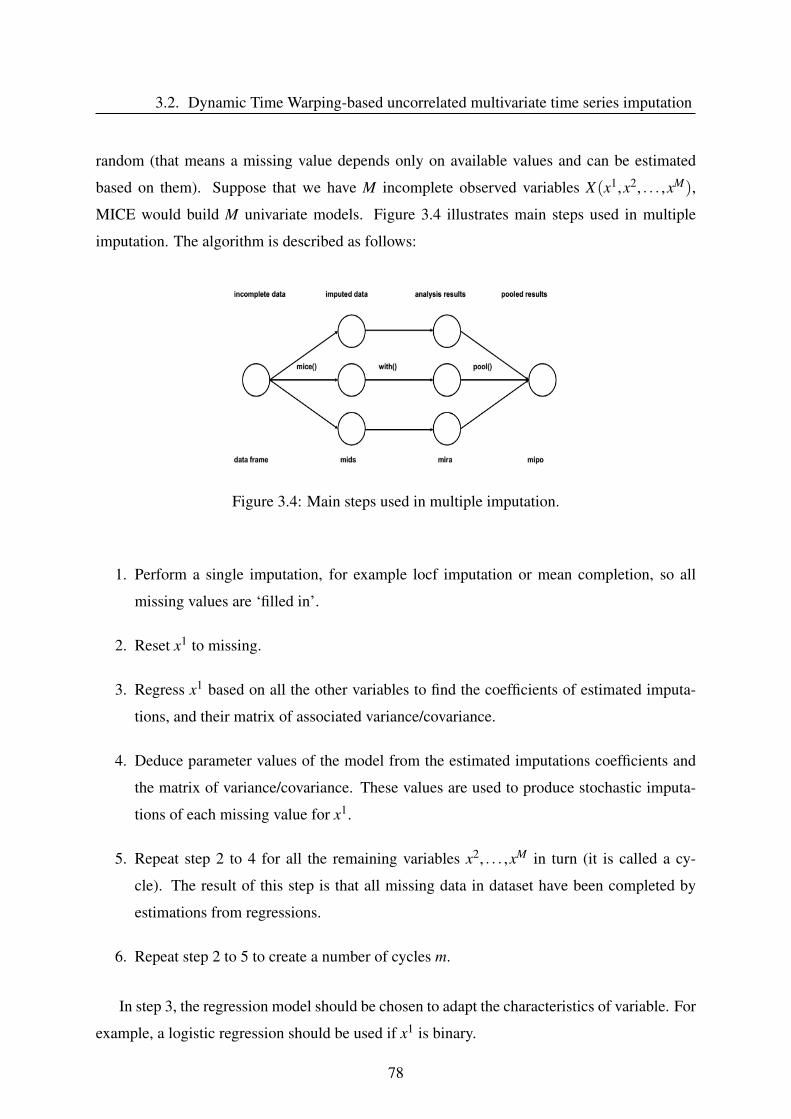
3.2. Dynamic Time Warping-based uncorrelated multivariate time series imputation
random (that means a missing value depends only on available values and can be estimated
based on them). Suppose that we have M incomplete observed variables X(x1,x2, . . . ,xM),
MICE would build M univariate models. Figure 3.4 illustrates main steps used in multiple
imputation. The algorithm is described as follows:
Figure 3.4: Main steps used in multiple imputation.
1. Perform a single imputation, for example locf imputation or mean completion, so all
missing values are ‘filled in’.
2. Reset x1 to missing.
3. Regress x1 based on all the other variables to find the coefficients of estimated imputa-
tions, and their matrix of associated variance/covariance.
4. Deduce parameter values of the model from the estimated imputations coefficients and
the matrix of variance/covariance. These values are used to produce stochastic imputa-
tions of each missing value for x1.
5. Repeat step 2 to 4 for all the remaining variables x2, . . . ,xM in turn (it is called a cy-
cle). The result of this step is that all missing data in dataset have been completed by
estimations from regressions.
6. Repeat step 2 to 5 to create a number of cycles m.
In step 3, the regression model should be chosen to adapt the characteristics of variable. For
example, a logistic regression should be used if x1 is binary.
78
CHAPTER 3. IMPUTATION APPROACHES FOR UNCORRELATED MULTIVARIATETIME SERIES
At the end of a cycle, one imputed data set is generated. This process is iterated m time to
produce m multiple data sets. And then these m sets are combined by applying rules of Rubin.
m parameter should be specified by the user.
Linear interpolation - na.approx (zoo package) [56]: This algorithm uses a generic func-
tion with interpolated values to estimate missing data.
missForest [76]: This approach is based on random forest algorithm to fill in missing data,
particularly in the case of mixed-type data. It involves 2 stages:
• The 1st stage: For each variable missForest builds a random forest model on the observed
part.
• The 2nd stage: The model, is built in the first stage, is used to predict missing values in
the variable.
The algorithm performs these two steps until a stopping criterion is met or the user specified
maximum of iterations is reached. The difference between the previous and the new imputation
data is computed after each iteration. The imputation process will stop as soon as the difference
has become larger once. In other words, the last imputation was less accurate than the previous
one. So, the final results are the imputation values of the before last iteration (excepting the
case that the user provides a number of iterations). For further details see [76].
3.2.3 Results and discussion
For evaluating the results, we apply the experiment protocol as previously defined in the chapter
1. In the present study, 7 missing data levels are considered on 3 datasets. Gaps are built at
rates 1%, 2%, 3%, 4%, 5%, 7.5% and 10% of the dataset size on every signal (here missing
sequences on each variable of the MAREL Carnot series correspond to around 15 days (353
consecutive missing) to 5 months (3,533 NAs)). For each missing ratio, the algorithms are
performed 5 times by randomly selecting the missing positions on the data. We then run 35
iterations for each data set.
Tables 3.1, 3.2 and 3.3 present the average performance evaluation of different imputation
algorithms for NNGC, simulated and MAREL Carnot time series for the 6 indicators. The best
results for each missing rate are highlighted in bold. These results confirm the good ability of
DTWUMI for filling missing values in uncorrelated multivariate time series.
NNGC dataset: Table 3.1 shows a comparison of five imputation methods on NNGC
dataset that has 7 missing ratios (1-10% missing values). We clearly find that missForest gives
79
3.2. Dynamic Time Warping-based uncorrelated multivariate time series imputation
the highest similarity, R2, FA2 and the lowest RMSE at every missing level. MICE is following
the missForest method on these indicators. However, when considering on other indices such
as FSD and FB, missForest only proves its performance at small missing rates (≤ 3%). At
larger missing levels (4%-7.5%), MICE provides the smallest FB indicator. And at 5%-10%
missing rates MI gives best FSD. A lower value indicates better performance. The results can
explain that NNGC dataset has high correlations between variables (approximate 0.79). MICE
and missForest estimate missing data based on other observed variables. That is why these
algorithms have better results and our algorithm does not prove its performance when complet-
ing datasets having high correlations. MI is also based on observed values for filling in missing
data but under an assumption that all variables follow a multivariate normal distribution. So
with this dataset, this method does not give good performance as MICE or missForest.
Simulated and MAREL Carnot datasets: From the results of tables 3.2 and 3.3, it is clear
that missForest, MI, and MICE do not demonstrate their performance for completing missing
data on these two datasets. For all missing rates, MissForest is ranked the second as consider-
ing similarity and RMSE indices (the simulation data) and the third or below for all indicators
(MAREL Carnot series). Because these two datasets have very low correlations between vari-
ables, especially for the simulated series which is an almost uncorrelated dataset. That explains
why, DTWUMI illustrates the best ability for imputation task: the highest similarity, R2, FA2
and the lowest RMSE, FSD for all missing ratios (table 3.5 - Simulated dataset). Regarding
MAREL Carnot series, this dataset has low correlations (around 0.2), so that our approach,
DTWUMI, does not show the capability to fill in missing values as it does in the simulated
dataset (table 3.6 - MAREL Carnot dataset). However, this method definitely indicates its im-
putation performance when considering similarity, R2, FA2, RMSE indicators at every missing
level. In particular, our method further proves the ability to fill in incomplete data with large
missing rates (7.5% and 10% on MAREL Carnot dataset). These gaps correspond to 110.4 and
147.2 days sampled at hourly frequency.
With the NNGC series (table 3.1), the na.approx method always produces the worst result
for every indicator. On the simulated and MAREL Carnot datasets, this method gives quite
good results when comparing the quantitative performance: the lowest FB and/or FSD at some
missing rates (simulated series), the second rank on similarity, R2, FA2 for all missing ratios
(MAREL Carnot dataset). However, when looking at the shape of imputation values generated
from of this method, it absolutely shows the worst shape (figure 3.5, 3.6).
In this study, we also carry out comparing the visualization performance of imputation val-
80
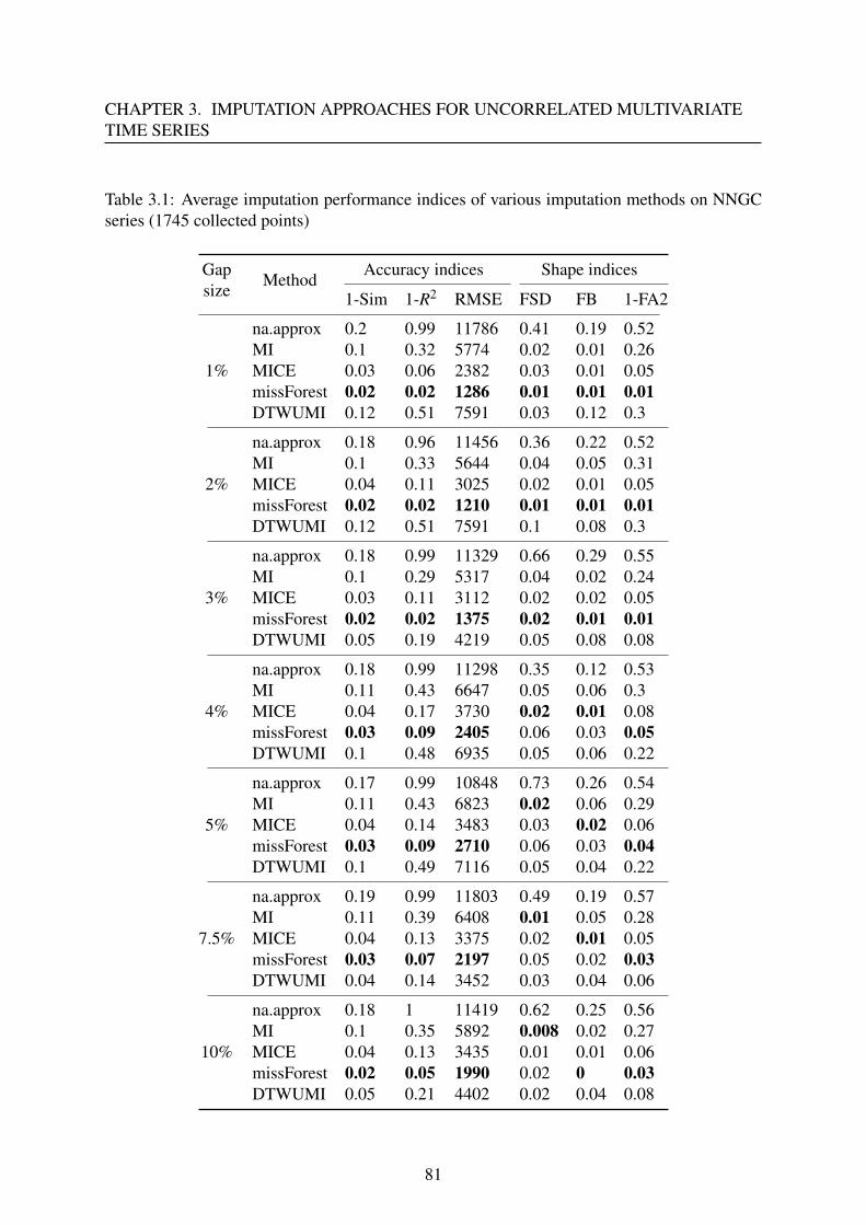
CHAPTER 3. IMPUTATION APPROACHES FOR UNCORRELATED MULTIVARIATETIME SERIES
Table 3.1: Average imputation performance indices of various imputation methods on NNGCseries (1745 collected points)
Gapsize
MethodAccuracy indices Shape indices
1-Sim 1-R2 RMSE FSD FB 1-FA2
1%
na.approx 0.2 0.99 11786 0.41 0.19 0.52MI 0.1 0.32 5774 0.02 0.01 0.26MICE 0.03 0.06 2382 0.03 0.01 0.05missForest 0.02 0.02 1286 0.01 0.01 0.01DTWUMI 0.12 0.51 7591 0.03 0.12 0.3
2%
na.approx 0.18 0.96 11456 0.36 0.22 0.52MI 0.1 0.33 5644 0.04 0.05 0.31MICE 0.04 0.11 3025 0.02 0.01 0.05missForest 0.02 0.02 1210 0.01 0.01 0.01DTWUMI 0.12 0.51 7591 0.1 0.08 0.3
3%
na.approx 0.18 0.99 11329 0.66 0.29 0.55MI 0.1 0.29 5317 0.04 0.02 0.24MICE 0.03 0.11 3112 0.02 0.02 0.05missForest 0.02 0.02 1375 0.02 0.01 0.01DTWUMI 0.05 0.19 4219 0.05 0.08 0.08
4%
na.approx 0.18 0.99 11298 0.35 0.12 0.53MI 0.11 0.43 6647 0.05 0.06 0.3MICE 0.04 0.17 3730 0.02 0.01 0.08missForest 0.03 0.09 2405 0.06 0.03 0.05DTWUMI 0.1 0.48 6935 0.05 0.06 0.22
5%
na.approx 0.17 0.99 10848 0.73 0.26 0.54MI 0.11 0.43 6823 0.02 0.06 0.29MICE 0.04 0.14 3483 0.03 0.02 0.06missForest 0.03 0.09 2710 0.06 0.03 0.04DTWUMI 0.1 0.49 7116 0.05 0.04 0.22
7.5%
na.approx 0.19 0.99 11803 0.49 0.19 0.57MI 0.11 0.39 6408 0.01 0.05 0.28MICE 0.04 0.13 3375 0.02 0.01 0.05missForest 0.03 0.07 2197 0.05 0.02 0.03DTWUMI 0.04 0.14 3452 0.03 0.04 0.06
10%
na.approx 0.18 1 11419 0.62 0.25 0.56MI 0.1 0.35 5892 0.008 0.02 0.27MICE 0.04 0.13 3435 0.01 0.01 0.06missForest 0.02 0.05 1990 0.02 0 0.03DTWUMI 0.05 0.21 4402 0.02 0.04 0.08
81
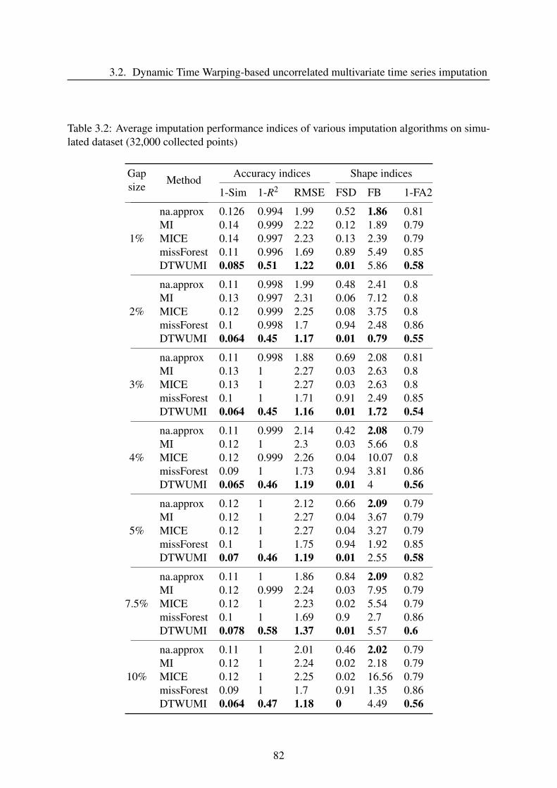
3.2. Dynamic Time Warping-based uncorrelated multivariate time series imputation
Table 3.2: Average imputation performance indices of various imputation algorithms on simu-lated dataset (32,000 collected points)
Gapsize
MethodAccuracy indices Shape indices
1-Sim 1-R2 RMSE FSD FB 1-FA2
1%
na.approx 0.126 0.994 1.99 0.52 1.86 0.81MI 0.14 0.999 2.22 0.12 1.89 0.79MICE 0.14 0.997 2.23 0.13 2.39 0.79missForest 0.11 0.996 1.69 0.89 5.49 0.85DTWUMI 0.085 0.51 1.22 0.01 5.86 0.58
2%
na.approx 0.11 0.998 1.99 0.48 2.41 0.8MI 0.13 0.997 2.31 0.06 7.12 0.8MICE 0.12 0.999 2.25 0.08 3.75 0.8missForest 0.1 0.998 1.7 0.94 2.48 0.86DTWUMI 0.064 0.45 1.17 0.01 0.79 0.55
3%
na.approx 0.11 0.998 1.88 0.69 2.08 0.81MI 0.13 1 2.27 0.03 2.63 0.8MICE 0.13 1 2.27 0.03 2.63 0.8missForest 0.1 1 1.71 0.91 2.49 0.85DTWUMI 0.064 0.45 1.16 0.01 1.72 0.54
4%
na.approx 0.11 0.999 2.14 0.42 2.08 0.79MI 0.12 1 2.3 0.03 5.66 0.8MICE 0.12 0.999 2.26 0.04 10.07 0.8missForest 0.09 1 1.73 0.94 3.81 0.86DTWUMI 0.065 0.46 1.19 0.01 4 0.56
5%
na.approx 0.12 1 2.12 0.66 2.09 0.79MI 0.12 1 2.27 0.04 3.67 0.79MICE 0.12 1 2.27 0.04 3.27 0.79missForest 0.1 1 1.75 0.94 1.92 0.85DTWUMI 0.07 0.46 1.19 0.01 2.55 0.58
7.5%
na.approx 0.11 1 1.86 0.84 2.09 0.82MI 0.12 0.999 2.24 0.03 7.95 0.79MICE 0.12 1 2.23 0.02 5.54 0.79missForest 0.1 1 1.69 0.9 2.7 0.86DTWUMI 0.078 0.58 1.37 0.01 5.57 0.6
10%
na.approx 0.11 1 2.01 0.46 2.02 0.79MI 0.12 1 2.24 0.02 2.18 0.79MICE 0.12 1 2.25 0.02 16.56 0.79missForest 0.09 1 1.7 0.91 1.35 0.86DTWUMI 0.064 0.47 1.18 0 4.49 0.56
82
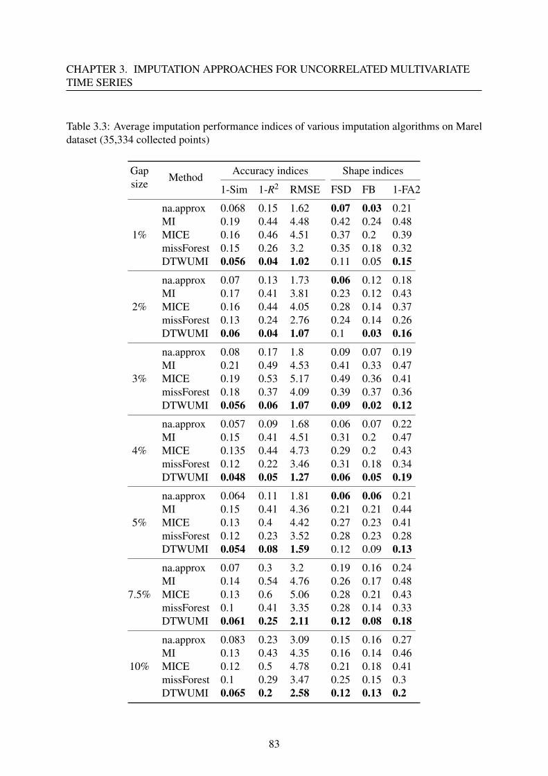
CHAPTER 3. IMPUTATION APPROACHES FOR UNCORRELATED MULTIVARIATETIME SERIES
Table 3.3: Average imputation performance indices of various imputation algorithms on Mareldataset (35,334 collected points)
Gapsize
MethodAccuracy indices Shape indices
1-Sim 1-R2 RMSE FSD FB 1-FA2
1%
na.approx 0.068 0.15 1.62 0.07 0.03 0.21MI 0.19 0.44 4.48 0.42 0.24 0.48MICE 0.16 0.46 4.51 0.37 0.2 0.39missForest 0.15 0.26 3.2 0.35 0.18 0.32DTWUMI 0.056 0.04 1.02 0.11 0.05 0.15
2%
na.approx 0.07 0.13 1.73 0.06 0.12 0.18MI 0.17 0.41 3.81 0.23 0.12 0.43MICE 0.16 0.44 4.05 0.28 0.14 0.37missForest 0.13 0.24 2.76 0.24 0.14 0.26DTWUMI 0.06 0.04 1.07 0.1 0.03 0.16
3%
na.approx 0.08 0.17 1.8 0.09 0.07 0.19MI 0.21 0.49 4.53 0.41 0.33 0.47MICE 0.19 0.53 5.17 0.49 0.36 0.41missForest 0.18 0.37 4.09 0.39 0.37 0.36DTWUMI 0.056 0.06 1.07 0.09 0.02 0.12
4%
na.approx 0.057 0.09 1.68 0.06 0.07 0.22MI 0.15 0.41 4.51 0.31 0.2 0.47MICE 0.135 0.44 4.73 0.29 0.2 0.43missForest 0.12 0.22 3.46 0.31 0.18 0.34DTWUMI 0.048 0.05 1.27 0.06 0.05 0.19
5%
na.approx 0.064 0.11 1.81 0.06 0.06 0.21MI 0.15 0.41 4.36 0.21 0.21 0.44MICE 0.13 0.4 4.42 0.27 0.23 0.41missForest 0.12 0.23 3.52 0.28 0.23 0.28DTWUMI 0.054 0.08 1.59 0.12 0.09 0.13
7.5%
na.approx 0.07 0.3 3.2 0.19 0.16 0.24MI 0.14 0.54 4.76 0.26 0.17 0.48MICE 0.13 0.6 5.06 0.28 0.21 0.43missForest 0.1 0.41 3.35 0.28 0.14 0.33DTWUMI 0.061 0.25 2.11 0.12 0.08 0.18
10%
na.approx 0.083 0.23 3.09 0.15 0.16 0.27MI 0.13 0.43 4.35 0.16 0.14 0.46MICE 0.12 0.5 4.78 0.21 0.18 0.41missForest 0.1 0.29 3.47 0.25 0.15 0.3DTWUMI 0.065 0.2 2.58 0.12 0.13 0.2
83
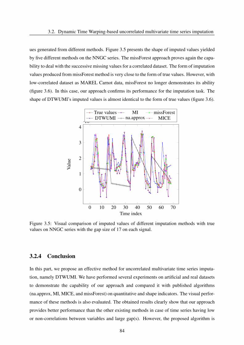
3.2. Dynamic Time Warping-based uncorrelated multivariate time series imputation
ues generated from different methods. Figure 3.5 presents the shape of imputed values yielded
by five different methods on the NNGC series. The missForest approach proves again the capa-
bility to deal with the successive missing values for a correlated dataset. The form of imputation
values produced from missForest method is very close to the form of true values. However, with
low-correlated dataset as MAREL Carnot data, missForest no longer demonstrates its ability
(figure 3.6). In this case, our approach confirms its performance for the imputation task. The
shape of DTWUMI’s imputed values is almost identical to the form of true values (figure 3.6).
0 10 20 30 40 50 60 70
0
1
2
3
4·104
Time index
Val
ue
True values MI missForestDTWUMI na.approx MICE
Figure 3.5: Visual comparison of imputed values of different imputation methods with truevalues on NNGC series with the gap size of 17 on each signal.
3.2.4 Conclusion
In this part, we propose an effective method for uncorrelated multivariate time series imputa-
tion, namely DTWUMI. We have performed several experiments on artificial and real datasets
to demonstrate the capability of our approach and compared it with published algorithms
(na.approx, MI, MICE, and missForest) on quantitative and shape indicators. The visual perfor-
mance of these methods is also evaluated. The obtained results clearly show that our approach
provides better performance than the other existing methods in case of time series having low
or non-correlations between variables and large gap(s). However, the proposed algorithm is
84
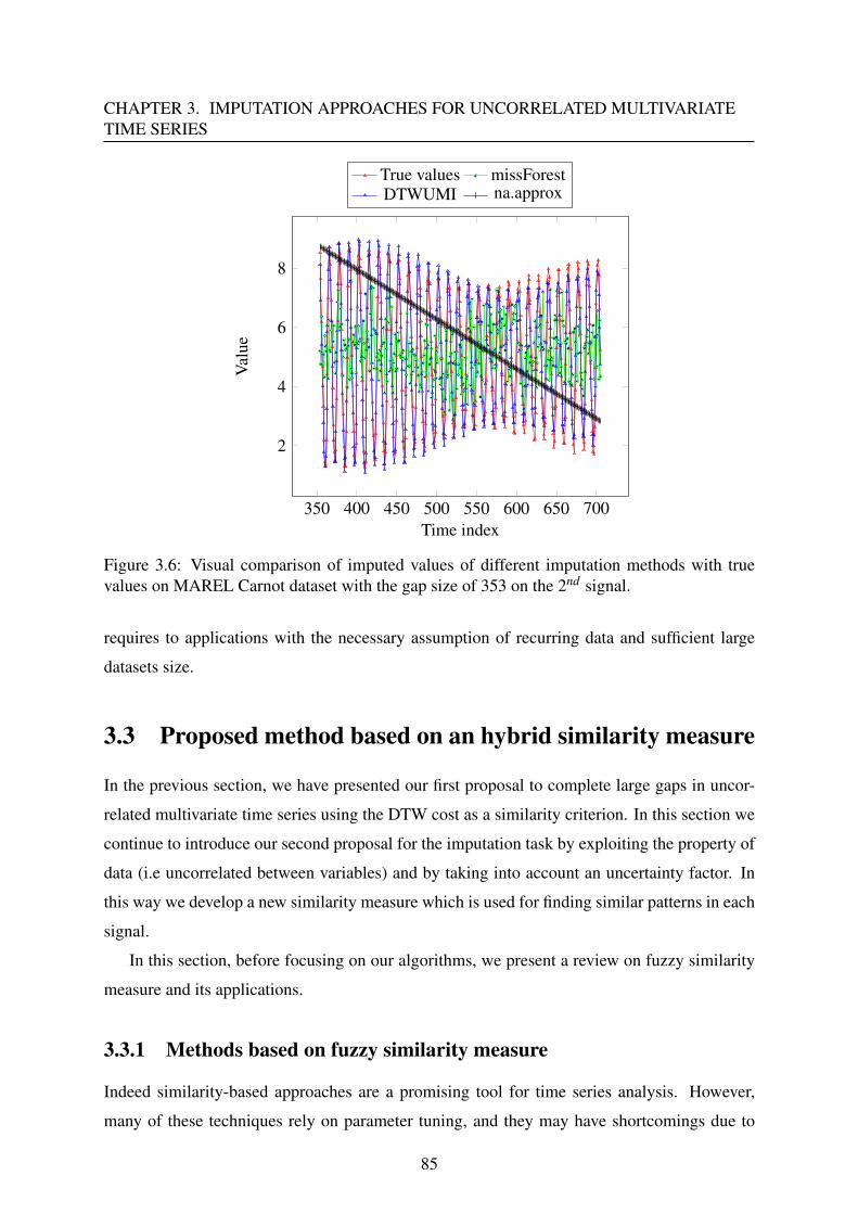
CHAPTER 3. IMPUTATION APPROACHES FOR UNCORRELATED MULTIVARIATETIME SERIES
350 400 450 500 550 600 650 700
2
4
6
8
Time index
Val
ue
True values missForestDTWUMI na.approx
Figure 3.6: Visual comparison of imputed values of different imputation methods with truevalues on MAREL Carnot dataset with the gap size of 353 on the 2nd signal.
requires to applications with the necessary assumption of recurring data and sufficient large
datasets size.
3.3 Proposed method based on an hybrid similarity measure
In the previous section, we have presented our first proposal to complete large gaps in uncor-
related multivariate time series using the DTW cost as a similarity criterion. In this section we
continue to introduce our second proposal for the imputation task by exploiting the property of
data (i.e uncorrelated between variables) and by taking into account an uncertainty factor. In
this way we develop a new similarity measure which is used for finding similar patterns in each
signal.
In this section, before focusing on our algorithms, we present a review on fuzzy similarity
measure and its applications.
3.3.1 Methods based on fuzzy similarity measure
Indeed similarity-based approaches are a promising tool for time series analysis. However,
many of these techniques rely on parameter tuning, and they may have shortcomings due to
85
3.3. Proposed method based on an hybrid similarity measure
dependencies between variables. The objective of this study is to fill large missing values in
uncorrelated multivariate time series. Thus, we have to deal with a high level of uncertainty.
There are many methods and theories to model uncertainties such as probabilistic models,
belief function theory [98], Dempster-Shafer [99], fuzzy sets [91], etc. Mikalsen et al. [100]
proposed to use GMM (Gaussian mixture models) and cluster kernel to deal with uncertainty.
This method needs ensemble learning with numerous learning datasets that are not available
in our case at the moment (marine data). So we have chosen to model this global uncertainty
using fuzzy sets (FS) introduced by Zadeh [91]. These techniques consider that measurements
have inherent imprecision rather than randomness.
Uncertainty is classically presented using three conceptually distinctive characteristics:
fuzziness, randomness and incompleteness. This classification is interesting for many applica-
tions, like sensor management (image processing, speech processing, time series processing)
and practical decision making. This paper focuses on (sensor) measurements treatment, but is
also relevant for other applications.
Incompleteness often affects time series prediction (time series obtained from marine data
such as salinity, temperature, ...). So it seems natural to use fuzzy similarity between sub-
sequences of time series to deal with these three kinds of uncertainties (fuzziness, randomness
and incompleteness). Fuzzy sets are now well-known and we only need to remind the basic
definition of "FS". Considering the universe X , a fuzzy set A ∈ X is characterized using a fuzzy
membership function µA:
µA : X → [0,1], (3.1)
where µA(x) represents the membership of x to A and is associated to the uncertainty of
x. In our case, we will consider similarity values between the sub-sequences as defined in the
following. One solution to deal with uncertainty brought by multivariate time series is to use the
concept of fuzzy time series [101]. In this framework, the variable observations are considered
as fuzzy numbers instead of real numbers. In our case the same modelling is used considering
distance measures between sub-sequences and then we compute the fuzzy similarities to find
the similar successive values in time series.
Fuzzy similarity is a generalization of the classical concept of equivalence and defines the
resemblance between two objects (here sub-sequences of time series). Similarity measures of
fuzzy values have been compared in [102] and have been extended in [16]. In [102], Pappis
and Karacapilidis presented three main kinds of similarity measures of fuzzy values, including:
86
CHAPTER 3. IMPUTATION APPROACHES FOR UNCORRELATED MULTIVARIATETIME SERIES
• measures based on the operations of union and intersection,
• measures based on the maximum difference,
• measures based on the difference and the sum of membership grades.
In [103, 104], the authors used these definitions to propose a distance metric for a space of
linguistic summaries based on fuzzy protoforms. Almeida et al. extended this work to put for-
ward linguistic summaries of categorical time series [105]. The introduced similarity measure
takes into account not only the linguistic meaning of the summaries, but also the numerical
characteristic attached to them. In the same way, Gupta et al. [15] introduced this approach to
create an hybrid similarity measure based on fuzzy logic. The approach is used to retrieve rel-
evant documents. In the other research, Al-Shamri and Al-Ashwal presented fuzzy weightings
of popular similarity measures for memory-based collaborative recommend systems [17].
Concerning the similarity between two sub-sequences of time series, we can use the DTW
cost as a similarity measure. However, to deal with the high level of uncertainty of the pro-
cessed signals, numerous similarity measures can be used to compute similarity like the cosine
similarity, Euclidean distance, Pearson correlation coefficient, and so on. Moreover, a fuzzy-
weighted combination of scores generated from different similarity measures could compara-
tively achieve better retrieval results than the use of a single similarity measure [15, 17].
Based on the same concepts, we propose to use a fuzzy rules interpolation scheme between
grades of membership of similarities fuzzy values. This method makes it possible to build a
new hybrid similarity measure for finding similar sub-sequence in time series.
3.3.2 FSMUMI-Proposed approach
The proposed imputation method is based on the retrieval and the similarity comparison of
available sub-sequences (namely Fuzzy Similarity Measure-based Uncorrelated Multivariate
Imputation, FSMUMI). In order to compare the sub-sequences, we create a new similarity
measure applying a multiple fuzzy rules interpolation.
Figure 3.7 demonstrates the mechanism of FSMUMI approach. Without loss of generality,
in this figure, we consider a multivariate time series including 3 variables whose correlations
are low.
The proposed approach involves three major stages. The first stage is to build two queries
Qa and Qb. The second stage is devoted to find the most similar windows to the queries.
87
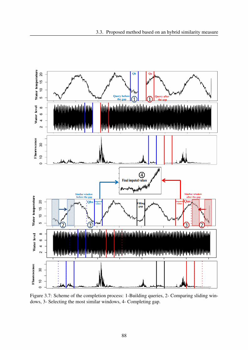
3.3. Proposed method based on an hybrid similarity measure
Figure 3.7: Scheme of the completion process: 1-Building queries, 2- Comparing sliding win-dows, 3- Selecting the most similar windows, 4- Completing gap.
88
CHAPTER 3. IMPUTATION APPROACHES FOR UNCORRELATED MULTIVARIATETIME SERIES
This stage includes two minor steps, comparing sliding windows to queries by using the new
similarity measure and selecting the similar windows Qas and Qbs. Finally, the imputation
values are computed by averaging values of the window following Qbs and the one preceding
Qas to complete the gap.
This method focus on filling large missing values in low/un-correlated multivariate time
series. For this type of data, we cannot take advantage of the relations between features to
estimate missing values. So we must base our approach on observed values on each signal
to complete missing data on itself. This means that we can complete missing data on each
variable, one by one. Further, an important point of our approach is that each incomplete signal
is processed as two separated time series, one time series before the considered gap and one
time series after this gap. This allows to increase the search space for similar values. Moreover,
applying the proposed process (one by one), FSMUMI makes it possible to handle the problem
of wholly missing variables (missing data at the same time index in the all variables).
In the next section, we present the way to compute the new similarity measure between
sub-sequences. Then, we provide details of the proposed approach to impute the successive
missing values of low/un-correlated multivariate time series.
3.3.2.1 Fuzzy weighted similarity measure between sub-sequences
To introduce a new similarity measure using multiple fuzzy rules interpolation to solve the
missing problem, two questions arise here: which measures will be taken as fuzzy? How can
they be "fuzzified"?
To answer the first question, we take into account 3 different distance measures between
two sub-sequences Q (Q = {qi, i = 1, · · · ,T}) and R (R = {ri, i = 1, · · · ,T}) including: Cosine
distance, Euclidean distance (these two measures are widely used in the literature) and Simi-
larity distance (this one was presented in our previous study [90]). These three measures are
defined as follows:
• Cosine distance is computed by eq 3.2. This coefficient presents the cosine of the angle
between Q and R
Cosine(Q,R) =∑
Ti=1 qi.ri
∑Ti=1(qi)2.∑T
i=1(ri)2(3.2)
89
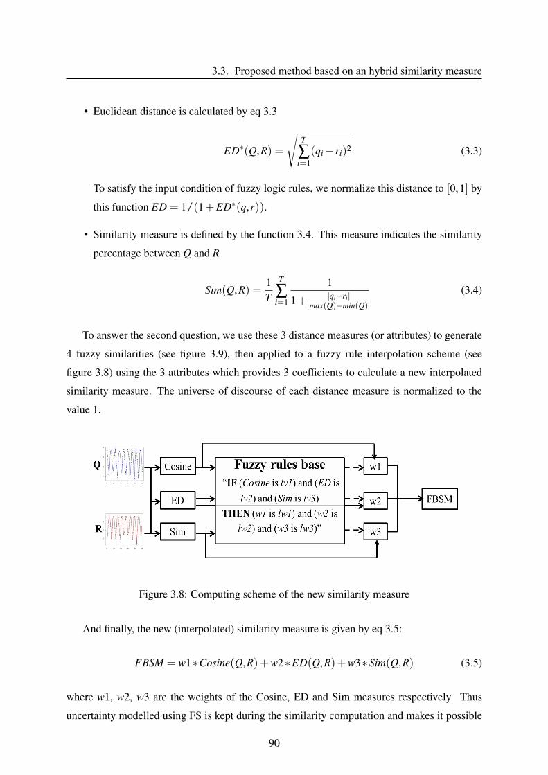
3.3. Proposed method based on an hybrid similarity measure
• Euclidean distance is calculated by eq 3.3
ED∗(Q,R) =
√T
∑i=1
(qi− ri)2 (3.3)
To satisfy the input condition of fuzzy logic rules, we normalize this distance to [0,1] by
this function ED = 1/(1+ED∗(q,r)).
• Similarity measure is defined by the function 3.4. This measure indicates the similarity
percentage between Q and R
Sim(Q,R) =1T
T
∑i=1
1
1+ |qi−ri|max(Q)−min(Q)
(3.4)
To answer the second question, we use these 3 distance measures (or attributes) to generate
4 fuzzy similarities (see figure 3.9), then applied to a fuzzy rule interpolation scheme (see
figure 3.8) using the 3 attributes which provides 3 coefficients to calculate a new interpolated
similarity measure. The universe of discourse of each distance measure is normalized to the
value 1.
Figure 3.8: Computing scheme of the new similarity measure
And finally, the new (interpolated) similarity measure is given by eq 3.5:
FBSM = w1∗Cosine(Q,R)+w2∗ED(Q,R)+w3∗Sim(Q,R) (3.5)
where w1, w2, w3 are the weights of the Cosine, ED and Sim measures respectively. Thus
uncertainty modelled using FS is kept during the similarity computation and makes it possible
90
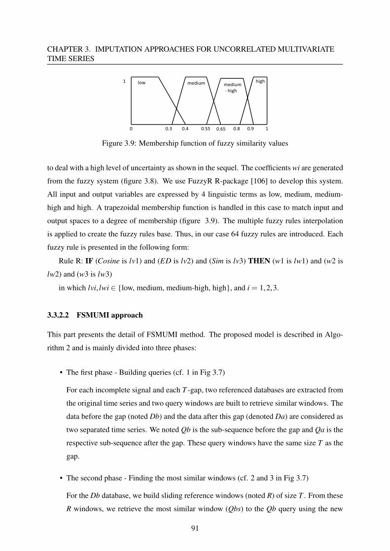
CHAPTER 3. IMPUTATION APPROACHES FOR UNCORRELATED MULTIVARIATETIME SERIES
0 0.3 0.55 0.65 0.9 1
1 low medium high
0.4 0.8
medium- high
Figure 3.9: Membership function of fuzzy similarity values
to deal with a high level of uncertainty as shown in the sequel. The coefficients wi are generated
from the fuzzy system (figure 3.8). We use FuzzyR R-package [106] to develop this system.
All input and output variables are expressed by 4 linguistic terms as low, medium, medium-
high and high. A trapezoidal membership function is handled in this case to match input and
output spaces to a degree of membership (figure 3.9). The multiple fuzzy rules interpolation
is applied to create the fuzzy rules base. Thus, in our case 64 fuzzy rules are introduced. Each
fuzzy rule is presented in the following form:
Rule R: IF (Cosine is lv1) and (ED is lv2) and (Sim is lv3) THEN (w1 is lw1) and (w2 is
lw2) and (w3 is lw3)
in which lvi, lwi ∈ {low, medium, medium-high, high}, and i = 1,2,3.
3.3.2.2 FSMUMI approach
This part presents the detail of FSMUMI method. The proposed model is described in Algo-
rithm 2 and is mainly divided into three phases:
• The first phase - Building queries (cf. 1 in Fig 3.7)
For each incomplete signal and each T -gap, two referenced databases are extracted from
the original time series and two query windows are built to retrieve similar windows. The
data before the gap (noted Db) and the data after this gap (denoted Da) are considered as
two separated time series. We noted Qb is the sub-sequence before the gap and Qa is the
respective sub-sequence after the gap. These query windows have the same size T as the
gap.
• The second phase - Finding the most similar windows (cf. 2 and 3 in Fig 3.7)
For the Db database, we build sliding reference windows (noted R) of size T . From these
R windows, we retrieve the most similar window (Qbs) to the Qb query using the new
91

3.3. Proposed method based on an hybrid similarity measure
Algorithm 2 FSMUMI algorithmInput: X = {x1,x2, . . . ,xM}: incomplete uncorrelated multivariate time series
N: size of time serest: index of a gap (position of the first missing of the gap)T : size of the gapstep_threshold: increment for finding a thresholdstep_sim_win: increment for finding a similar window
Output: Y - completed (imputed) time series1: for each incomplete signal x j ∈ X do2: for each gap at t index in x j do3: Divide x j into two separated time series Da, Db: Da = x j[t +T : N],Db = x j[1 : t−1]4: Completing all lines containing missing parameter on Da,Db by a max trapezoid function5: Construct queries Qa, Qb-temporal windows after and before the gap Qa = Da[1 : T ], Qb = Db[t−T +1 :
t−1]6: for Db data do7: Step a: Find the threshold in the Db database8: i← 1; FSM← NULL9: while i≤ length(Db) do
10: k← i+T −111: Create a reference window: R(i) = Db[i : k]12: Calculate a fuzzy-based similarity measure between Qb and R(i): f bsm13: Save the f bsm to FMS14: i← i+ step_threshold15: end while16: return threshold = max{FBMS}17: Step b: Find similar windows in the Db database18: i← 1; Lopb← NULL19: while i≤ length(Db) do20: k← i+T −121: Create a reference window: R(i) = Db[i : k]22: Calculate a fuzzy-based similarity measure between Qb and R(i): f bsm23: if f bsm≥ threshold then24: Save position of R(i) to Lopb25: end if26: i← i+ step_sim_win27: end while28: return position of Qbs - the most similar window to Qb having the maximum fuzzy similarity measure in
the Lopb list.29: end for30: for Da data do31: Perform Step a and Step b for Da data32: return position of Qas - the most similar window to Qa33: end for34: Replace the missing values at the position t by average vector of the window after Qbs and the one previous
Qas35: end for36: end for37: return Y - imputed time series
92
CHAPTER 3. IMPUTATION APPROACHES FOR UNCORRELATED MULTIVARIATETIME SERIES
similarity measure f bsm as previously defined in subsection 3.3.2.1. Details are in the
following:
We first find the threshold, which allows to consider two windows to be similar. For each
increment step_threshold, we compute a f bsm similarity measure between a sliding
window R and the query Qb. The threshold is the maximum value obtained from the all
f bsm calculated ( Step a: in Algorithm 2).
We then find the most similar window to the Qb query. For each increment similar
window step_sim_win, a f bsm of a R sliding reference and the Qb query is estimated.
We then compare this f bsm to the threshold to determine if this R reference is similar to
the Qb query. We finally choose the most similar window Qbs with the maximum f bsm
of all the similar windows ( Step b: in Algorithm 2).
The same process is performed to find the most similar window Qas in Da data.
In the proposed approach, the dynamics and the shape of data before and after a gap are
a key-point. This means that we take into account both queries Qa (after the gap) and Qb
(before the gap). This makes it possible to find out windows that have the most similar
dynamics and shape to the queries.
• The third phase (cf. 4 in Fig 3.7)
When results from both referenced time series are available, we fill in the gap by averag-
ing values of the window previous Qas and the one following Qbs. The average values
are used in our approach because model averaging makes the final results more stable
and unbiased [107].
3.3.3 Validation procedure
To analyze the relevance of the proposed approach, it is important to compare with state-of-
the-art methods. This validation step will be conducted on the main application of this thesis.
Our approach is compared with well-known methods (including Amelia II, FcM, MI, MICE,
missForest, na.approx, and DTWUMI) and experiments are performed on three multivariate
time series with the same protocol and the same gaps. The experiments process includes 3 steps
as previously mentioned in Chapter 1. These methods are assessed in terms of their efficacy
of accuracy and shape between true values and completion data using criteria for evaluation
93
3.3. Proposed method based on an hybrid similarity measure
as defined in Chapter 1. The datasets and multivariate time series imputation methods are
described in detail below.
3.3.3.1 Datasets description
For assessment of the proposed approach and comparison of its performance to several pub-
lished algorithms, we use 3 multivariate time series, one from UCI Machine Learning reposi-
tory, one simulated dataset (this allows us to handle the correlations between variables and per-
centage of missing values) and finally a real time series hourly sampled by IFREMER (France)
in the eastern English Channel. The two last datasets (Simulated dataset and MAREL-Carnot
dataset) have been mentioned in the previous part (DTWUMI).
• Synthetic dataset [108]: The data are synthetic time series, including 10 features, 100,000
sampled points. All data points are in the range -0.5 to +0.5. The data appear highly pe-
riodic, but never exactly repeat. They have structure at different resolutions. Each of the
10 features is generated by independent invocations of the function:
y =7
∑i=3
12i sin(2π(22+i + rand(2i))t);0≤ t ≤ 1 (3.6)
where rand(x) produces a random integer between 0 and x.
These data are very large so we choose only a subset of 3 signals for performing experi-
ments.
• Simulated dataset: see the section 3.2.2.1.
• MAREL-Carnot dataset: see the section 3.2.2.1.
3.3.3.2 Multivariate imputation approaches
In the present study, we perform a comparison of the proposed algorithm with 7 other ap-
proaches (comprising Amelia II, FCM, MI, MICE, missForest, na.approx, and DTWUMI) for
the imputation of multivariate time series. We use R language to execute all these algorithms.
1. Amelia II (Amelia II R-package) [109]: This method supposes that all the variables in
a dataset have Multivariate Normal Distribution (MVN) and missing data are Missing at
Random. Figure 3.10 illustrates different steps of this approach.
94
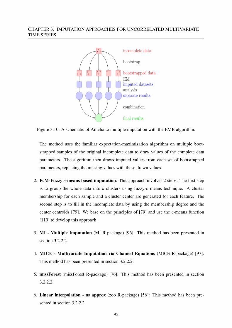
CHAPTER 3. IMPUTATION APPROACHES FOR UNCORRELATED MULTIVARIATETIME SERIES
Figure 3.10: A schematic of Amelia to multiple imputation with the EMB algorithm.
The method uses the familiar expectation-maximization algorithm on multiple boot-
strapped samples of the original incomplete data to draw values of the complete data
parameters. The algorithm then draws imputed values from each set of bootstrapped
parameters, replacing the missing values with these drawn values.
2. FcM-Fuzzy c-means based imputation: This approach involves 2 steps. The first step
is to group the whole data into k clusters using fuzzy-c means technique. A cluster
membership for each sample and a cluster center are generated for each feature. The
second step is to fill in the incomplete data by using the membership degree and the
center centroids [79]. We base on the principles of [79] and use the c-means function
[110] to develop this approach.
3. MI - Multiple Imputation (MI R-package) [96]: This method has been presented in
section 3.2.2.2.
4. MICE - Multivariate Imputation via Chained Equations (MICE R-package) [97]:
This method has been presented in section 3.2.2.2.
5. missForest (missForest R-package) [76]: This method has been presented in section
3.2.2.2.
6. Linear interpolation - na.approx (zoo R-package) [56]: This method has been pre-
sented in section 3.2.2.2.
95
3.3. Proposed method based on an hybrid similarity measure
7. DTWUMI [111]: In the previous section, we have introduced details of this method.
3.3.4 Results and discussion
In comparison with our previous proposal and state-of-the art approaches, we implemented the
same protocol and evaluation criteria: seven missing data levels on three large uncorrelated
datasets. On each signal, we build simulated gaps in the complete signal with different rates
ranging from 1%, 2%, 3%, 4%, 5%, 7.5% and 10% of the data (here the biggest gap of synthetic
dataset is 10,000 missing values). For every missing ratio, the approaches are run 5 times by
randomly choosing the positions of missing on the data. We then perform 35 iterations for each
dataset.
This section provides experiment results obtained from the proposed approach and com-
pares its ability with the seven published approaches. Results are discussed in three parts, i.e
quantitative performance, visual performance and execution times.
3.3.4.1 Quantitative performance comparison
Tables 3.4, 3.5, 3.6 illustrate the average ability of various imputation methods for synthetic,
simulated and MAREL-Carnot time series using 6 measurements as previously defined. For
each missing level, the best results are highlighted in bold. These results demonstrate the
improved performance of FSMUMI to complete missing data in low/uncorrelated multivariate
time series.
Synthetic dataset: Table 3.4 presents a comparison of 8 imputation methods on synthetic
dataset that contains 7 missing data levels (1-10%). The results clearly show that when a gap
size is greater than 2%, the proposed method yields the highest similarity, R2, FA2 and the
lowest RMSE, FB. With this dataset, na.approx gives the best performance at the smallest
missing data level for all indices and is ranked second for other ratios of missing values (2-
5%) for similarity and FA2, RMSE (2-4%), and R2 (the 1st rank at 2% missing rate, the 2nd at
3%, 5%). The results can explain that the synthetic data are generated by a function (eq. 3.6).
na.approx method which applies the interpolation function to estimate missing values. So it is
easy to find a function to generate values that are approximate real values when missing data
rates are small. But this work is more difficult when the missing sample size rises, that is why
the ability of na.approx decreases as missing data levels increase, especially at 7.5% and 10%
rates. Although this dataset never exactly repeats itself and our approach is proposed under
96

CHAPTER 3. IMPUTATION APPROACHES FOR UNCORRELATED MULTIVARIATETIME SERIES
the assumption of recurrent data but the FSMUMI approach proves its performance for the
imputation task even if the missing size increases.
Among the considered methods, the FcM-based approach is less accurate at lower missing
rates but it provides better results at larger missing ratios as regards the accuracy indices.
Table 3.4: Average imputation performance indices of various imputation algorithms on syn-thetic dataset (100,000 collected points)
Gap
sizeMethod
Accuracy indices Shape indices
1-Sim 1-R2 RMSE FSD FB 1-FA2
1%
FSMUMI 0.136 0.261 0.051 0.358 3.253 0.364
Amelia 0.275 0.999 0.143 0.409 2.252 0.773
FcM 0.231 0.722 0.096 1.889 2.208 0.996
MI 0.275 0.999 0.142 0.421 2.091 0.773
MICE 0.258 0.944 0.13 0.406 2.452 0.72
missForest 0.248 0.915 0.122 0.389 3.976 0.744
na.approx 0.052 0.066 0.019 0.054 0.29 0.074
DTWUMI 0.257 0.713 0.88 0.725 0.405 0.69
2%
FSMUMI 0.1 0.295 0.046 0.155 0.395 0.337
Amelia 0.259 0.998 0.147 0.275 2.005 0.803
FcM 0.208 0.686 0.104 1.863 2.289 0.987
MI 0.259 0.998 0.147 0.268 2.11 0.81
MICE 0.244 0.968 0.14 0.255 7.616 0.759
missForest 0.239 0.968 0.133 0.279 3.156 0.792
na.approx 0.104 0.278 0.047 0.224 0.398 0.347
DTWUMI 0.237 0.775 0.867 0.509 8.449 0.646
3%
FSMUMI 0.113 0.341 0.056 0.219 0.852 0.322
Amelia 0.218 0.911 0.127 0.133 6.128 0.76
FcM 0.214 0.601 0.1 1.832 1.759 0.989
MI 0.253 0.993 0.141 0.236 2.295 0.775
MICE 0.21 0.873 0.118 0.208 5.118 0.703
missForest 0.188 0.796 0.102 0.215 1.846 0.627
na.approx 0.148 0.43 0.072 0.372 2.382 0.577
DTWUMI 0.231 0.799 0.874 0.332 27.952 0.69
4%
FSMUMI 0.06 0.146 0.037 0.099 0.738 0.299
Amelia 0.208 1 0.14 0.213 2.171 0.807
FcM 0.155 0.759 0.095 1.85 2.09 0.986
MI 0.208 0.999 0.14 0.196 2.302 0.807
97
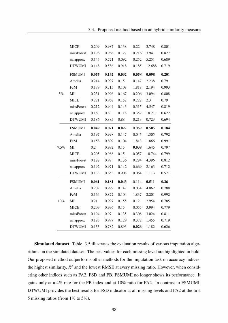
3.3. Proposed method based on an hybrid similarity measure
MICE 0.209 0.987 0.138 0.22 3.748 0.801
missForest 0.196 0.968 0.127 0.216 3.94 0.827
na.approx 0.145 0.721 0.092 0.252 5.251 0.689
DTWUMI 0.148 0.586 0.918 0.185 12.688 0.719
5%
FSMUMI 0.055 0.132 0.032 0.058 0.098 0.201
Amelia 0.214 0.997 0.15 0.147 2.238 0.79
FcM 0.179 0.715 0.108 1.818 2.194 0.993
MI 0.231 0.996 0.167 0.206 3.094 0.808
MICE 0.221 0.968 0.152 0.222 2.3 0.79
missForest 0.212 0.944 0.143 0.315 4.547 0.819
na.approx 0.16 0.8 0.118 0.352 18.217 0.622
DTWUMI 0.186 0.885 0.88 0.213 0.723 0.694
7.5%
FSMUMI 0.049 0.071 0.027 0.069 0.505 0.184
Amelia 0.197 0.998 0.147 0.045 1.305 0.792
FcM 0.158 0.809 0.104 1.813 1.866 0.991
MI 0.2 0.992 0.15 0.038 1.645 0.797
MICE 0.205 0.988 0.15 0.057 10.744 0.799
missForest 0.188 0.97 0.136 0.284 4.396 0.812
na.approx 0.192 0.971 0.142 0.669 2.163 0.712
DTWUMI 0.133 0.653 0.908 0.064 1.113 0.571
10%
FSMUMI 0.061 0.181 0.043 0.114 0.511 0.26
Amelia 0.202 0.999 0.147 0.034 4.062 0.788
FcM 0.164 0.872 0.104 1.837 2.201 0.992
MI 0.21 0.997 0.155 0.12 2.954 0.785
MICE 0.209 0.996 0.15 0.055 3.994 0.779
missForest 0.194 0.97 0.135 0.308 3.024 0.811
na.approx 0.183 0.997 0.129 0.372 1.455 0.719
DTWUMI 0.155 0.782 0.893 0.026 1.182 0.626
Simulated dataset: Table 3.5 illustrates the evaluation results of various imputation algo-
rithms on the simulated dataset. The best values for each missing level are highlighted in bold.
Our proposed method outperforms other methods for the imputation task on accuracy indices:
the highest similarity, R2 and the lowest RMSE at every missing ratio. However, when consid-
ering other indices such as FA2, FSD and FB, FSMUMI no longer shows its performance. It
gains only at a 4% rate for the FB index and at 10% ratio for FA2. In contrast to FSMUMI,
DTWUMI provides the best results for FSD indicator at all missing levels and FA2 at the first
5 missing ratios (from 1% to 5%).
98
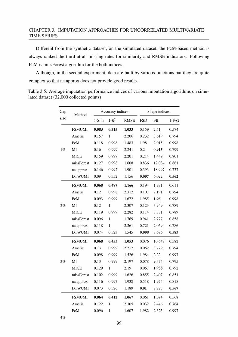
CHAPTER 3. IMPUTATION APPROACHES FOR UNCORRELATED MULTIVARIATETIME SERIES
Different from the synthetic dataset, on the simulated dataset, the FcM-based method is
always ranked the third at all missing rates for similarity and RMSE indicators. Following
FcM is missForest algorithm for the both indices.
Although, in the second experiment, data are built by various functions but they are quite
complex so that na.approx does not provide good results.
Table 3.5: Average imputation performance indices of various imputation algorithms on simu-lated dataset (32,000 collected points)
Gap
sizeMethod
Accuracy indices Shape indices
1-Sim 1-R2 RMSE FSD FB 1-FA2
1%
FSMUMI 0.083 0.515 1.033 0.159 2.51 0.574
Amelia 0.157 1 2.206 0.232 3.619 0.794
FcM 0.118 0.998 1.483 1.98 2.015 0.998
MI 0.16 0.999 2.241 0.2 0.915 0.799
MICE 0.159 0.998 2.201 0.214 1.449 0.801
missForest 0.127 0.998 1.608 0.836 12.034 0.861
na.approx 0.146 0.992 1.901 0.393 18.997 0.777
DTWUMI 0.09 0.552 1.156 0.007 6.022 0.562
2%
FSMUMI 0.068 0.487 1.166 0.194 1.971 0.611
Amelia 0.12 0.998 2.312 0.107 2.191 0.794
FcM 0.093 0.999 1.672 1.985 1.96 0.998
MI 0.12 1 2.307 0.123 3.949 0.789
MICE 0.119 0.999 2.282 0.114 8.881 0.789
missForest 0.096 1 1.769 0.941 2.777 0.858
na.approx 0.118 1 2.261 0.721 2.059 0.786
DTWUMI 0.074 0.523 1.545 0.008 3.686 0.583
3%
FSMUMI 0.068 0.453 1.053 0.076 10.649 0.582
Amelia 0.13 0.999 2.212 0.062 3.779 0.794
FcM 0.098 0.999 1.526 1.984 2.22 0.997
MI 0.13 0.999 2.197 0.078 9.374 0.795
MICE 0.129 1 2.19 0.067 1.938 0.792
missForest 0.102 0.999 1.626 0.855 2.407 0.851
na.approx 0.116 0.997 1.938 0.518 1.974 0.818
DTWUMI 0.073 0.526 1.189 0.01 8.725 0.567
4%
FSMUMI 0.064 0.412 1.067 0.061 1.374 0.568
Amelia 0.122 1 2.305 0.032 2.446 0.764
FcM 0.096 1 1.607 1.982 2.325 0.997
99
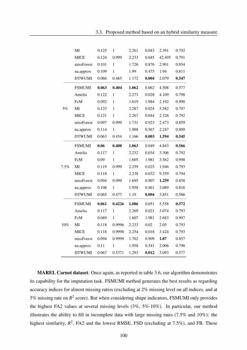
3.3. Proposed method based on an hybrid similarity measure
MI 0.125 1 2.261 0.043 2.391 0.792
MICE 0.124 0.999 2.233 0.045 42.495 0.791
missForest 0.101 1 1.726 0.876 2.901 0.854
na.approx 0.109 1 1.99 0.475 1.94 0.811
DTWUMI 0.066 0.465 1.172 0.004 2.079 0.547
5%
FSMUMI 0.063 0.404 1.062 0.062 4.508 0.577
Amelia 0.122 1 2.273 0.028 4.109 0.798
FcM 0.092 1 1.619 1.984 2.192 0.998
MI 0.123 1 2.287 0.024 5.582 0.797
MICE 0.121 1 2.267 0.044 2.326 0.792
missForest 0.097 0.999 1.731 0.923 2.473 0.859
na.approx 0.114 1 1.988 0.567 2.247 0.809
DTWUMI 0.063 0.454 1.166 0.003 1.594 0.545
7.5%
FSMUMI 0.06 0.408 1.063 0.049 4.843 0.566
Amelia 0.117 1 2.232 0.034 3.306 0.792
FcM 0.09 1 1.605 1.981 3.562 0.998
MI 0.119 0.999 2.259 0.025 1.946 0.793
MICE 0.118 1 2.238 0.032 9.359 0.794
missForest 0.094 0.999 1.695 0.907 1.259 0.858
na.approx 0.108 1 1.958 0.461 3.089 0.816
DTWUMI 0.065 0.477 1.19 0.004 3.851 0.566
10%
FSMUMI 0.061 0.4226 1.086 0.051 5.558 0.572
Amelia 0.117 1 2.269 0.021 3.074 0.793
FcM 0.089 1 1.607 1.981 2.683 0.997
MI 0.118 0.9996 2.233 0.02 2.05 0.793
MICE 0.118 0.9998 2.254 0.018 3.424 0.793
missForest 0.094 0.9999 1.702 0.909 1.87 0.857
na.approx 0.11 1 1.958 0.541 2.006 0.798
DTWUMI 0.067 0.5371 1.293 0.012 3.093 0.577
MAREL Carnot dataset: Once again, as reported in table 3.6, our algorithm demonstrates
its capability for the imputation task. FSMUMI method generates the best results as regarding
accuracy indices for almost missing ratios (excluding at 2% missing level on all indices, and at
5% missing rate on R2 score). But when considering shape indicators, FSMUMI only provides
the highest FA2 values at several missing levels (3%, 5%-10%). In particular, our method
illustrates the ability to fill in incomplete data with large missing rates (7.5% and 10%): the
highest similarity, R2, FA2 and the lowest RMSE, FSD (excluding at 7.5%), and FB. These
100
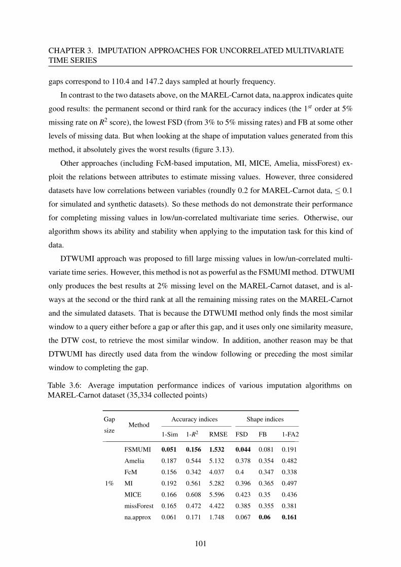
CHAPTER 3. IMPUTATION APPROACHES FOR UNCORRELATED MULTIVARIATETIME SERIES
gaps correspond to 110.4 and 147.2 days sampled at hourly frequency.
In contrast to the two datasets above, on the MAREL-Carnot data, na.approx indicates quite
good results: the permanent second or third rank for the accuracy indices (the 1st order at 5%
missing rate on R2 score), the lowest FSD (from 3% to 5% missing rates) and FB at some other
levels of missing data. But when looking at the shape of imputation values generated from this
method, it absolutely gives the worst results (figure 3.13).
Other approaches (including FcM-based imputation, MI, MICE, Amelia, missForest) ex-
ploit the relations between attributes to estimate missing values. However, three considered
datasets have low correlations between variables (roundly 0.2 for MAREL-Carnot data, ≤ 0.1
for simulated and synthetic datasets). So these methods do not demonstrate their performance
for completing missing values in low/un-correlated multivariate time series. Otherwise, our
algorithm shows its ability and stability when applying to the imputation task for this kind of
data.
DTWUMI approach was proposed to fill large missing values in low/un-correlated multi-
variate time series. However, this method is not as powerful as the FSMUMI method. DTWUMI
only produces the best results at 2% missing level on the MAREL-Carnot dataset, and is al-
ways at the second or the third rank at all the remaining missing rates on the MAREL-Carnot
and the simulated datasets. That is because the DTWUMI method only finds the most similar
window to a query either before a gap or after this gap, and it uses only one similarity measure,
the DTW cost, to retrieve the most similar window. In addition, another reason may be that
DTWUMI has directly used data from the window following or preceding the most similar
window to completing the gap.
Table 3.6: Average imputation performance indices of various imputation algorithms onMAREL-Carnot dataset (35,334 collected points)
Gap
sizeMethod
Accuracy indices Shape indices
1-Sim 1-R2 RMSE FSD FB 1-FA2
1%
FSMUMI 0.051 0.156 1.532 0.044 0.081 0.191
Amelia 0.187 0.544 5.132 0.378 0.354 0.482
FcM 0.156 0.342 4.037 0.4 0.347 0.338
MI 0.192 0.561 5.282 0.396 0.365 0.497
MICE 0.166 0.608 5.596 0.423 0.35 0.436
missForest 0.165 0.472 4.422 0.385 0.355 0.381
na.approx 0.061 0.171 1.748 0.067 0.06 0.161
101
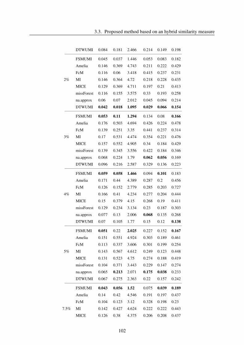
3.3. Proposed method based on an hybrid similarity measure
DTWUMI 0.084 0.181 2.466 0.214 0.149 0.198
2%
FSMUMI 0.045 0.037 1.446 0.053 0.083 0.182
Amelia 0.146 0.369 4.743 0.211 0.222 0.429
FcM 0.116 0.06 3.418 0.415 0.237 0.231
MI 0.146 0.364 4.72 0.218 0.228 0.435
MICE 0.129 0.369 4.711 0.197 0.21 0.413
missForest 0.116 0.155 3.575 0.33 0.193 0.258
na.approx 0.06 0.07 2.012 0.045 0.094 0.214
DTWUMI 0.042 0.018 1.095 0.029 0.066 0.154
3%
FSMUMI 0.053 0.11 1.294 0.134 0.08 0.166
Amelia 0.176 0.503 4.694 0.426 0.224 0.478
FcM 0.139 0.251 3.35 0.441 0.237 0.314
MI 0.17 0.531 4.474 0.354 0.221 0.476
MICE 0.157 0.552 4.905 0.34 0.184 0.429
missForest 0.139 0.345 3.556 0.422 0.184 0.346
na.approx 0.068 0.224 1.79 0.062 0.056 0.169
DTWUMI 0.096 0.216 2.587 0.329 0.136 0.223
4%
FSMUMI 0.059 0.058 1.466 0.094 0.101 0.183
Amelia 0.171 0.44 4.389 0.287 0.2 0.456
FcM 0.126 0.152 2.779 0.285 0.203 0.727
MI 0.166 0.41 4.234 0.277 0.204 0.444
MICE 0.15 0.379 4.15 0.268 0.19 0.411
missForest 0.129 0.234 3.134 0.23 0.187 0.303
na.approx 0.077 0.13 2.006 0.068 0.135 0.268
DTWUMI 0.07 0.105 1.77 0.15 0.12 0.138
5%
FSMUMI 0.051 0.22 2.025 0.227 0.152 0.167
Amelia 0.151 0.551 4.924 0.303 0.189 0.461
FcM 0.113 0.337 3.606 0.301 0.199 0.254
MI 0.143 0.567 4.612 0.249 0.123 0.448
MICE 0.131 0.523 4.75 0.274 0.188 0.419
missForest 0.104 0.371 3.443 0.229 0.147 0.274
na.approx 0.065 0.213 2.071 0.175 0.038 0.233
DTWUMI 0.067 0.275 2.363 0.22 0.157 0.242
7.5%
FSMUMI 0.043 0.056 1.52 0.075 0.039 0.189
Amelia 0.14 0.42 4.546 0.191 0.197 0.437
FcM 0.104 0.123 3.12 0.328 0.198 0.23
MI 0.142 0.427 4.624 0.222 0.222 0.443
MICE 0.126 0.38 4.375 0.206 0.208 0.437
102
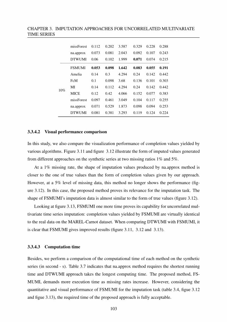
CHAPTER 3. IMPUTATION APPROACHES FOR UNCORRELATED MULTIVARIATETIME SERIES
missForest 0.112 0.202 3.587 0.329 0.228 0.288
na.approx 0.073 0.081 2.043 0.092 0.107 0.243
DTWUMI 0.06 0.102 1.999 0.071 0.074 0.215
10%
FSMUMI 0.053 0.098 1.642 0.083 0.055 0.191
Amelia 0.14 0.3 4.294 0.24 0.142 0.442
FcM 0.1 0.098 3.68 0.136 0.101 0.303
MI 0.14 0.112 4.294 0.24 0.142 0.442
MICE 0.12 0.42 4.066 0.152 0.077 0.383
missForest 0.097 0.461 3.049 0.104 0.117 0.255
na.approx 0.071 0.529 1.873 0.098 0.094 0.253
DTWUMI 0.081 0.381 3.293 0.119 0.124 0.224
3.3.4.2 Visual performance comparison
In this study, we also compare the visualization performance of completion values yielded by
various algorithms. Figure 3.11 and figure 3.12 illustrate the form of imputed values generated
from different approaches on the synthetic series at two missing ratios 1% and 5%.
At a 1% missing rate, the shape of imputation values produced by na.approx method is
closer to the one of true values than the form of completion values given by our approach.
However, at a 5% level of missing data, this method no longer shows the performance (fig-
ure 3.12). In this case, the proposed method proves its relevance for the imputation task. The
shape of FSMUMI’s imputation data is almost similar to the form of true values (figure 3.12).
Looking at figure 3.13, FSMUMI one more time proves its capability for uncorrelated mul-
tivariate time series imputation: completion values yielded by FSMUMI are virtually identical
to the real data on the MAREL-Carnot dataset. When comparing DTWUMI with FSMUMI, it
is clear that FSMUMI gives improved results (figure 3.11, 3.12 and 3.13).
3.3.4.3 Computation time
Besides, we perform a comparison of the computational time of each method on the synthetic
series (in second - s). Table 3.7 indicates that na.approx method requires the shortest running
time and DTWUMI approach takes the longest computing time. The proposed method, FS-
MUMI, demands more execution time as missing rates increase. However, considering the
quantitative and visual performance of FSMUMI for the imputation task (table 3.4, figue 3.12
and figue 3.13), the required time of the proposed approach is fully acceptable.
103
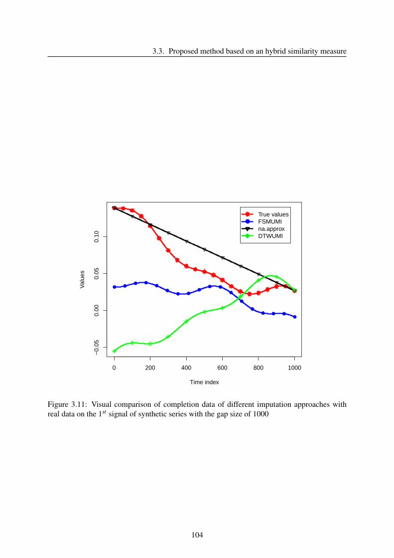
3.3. Proposed method based on an hybrid similarity measure
0 200 400 600 800 1000
−0.
050.
000.
050.
10
Time index
Val
ues
● ●● ●
●
●● ●
●● ●
●
●
●● ● ●
●
●
True valuesFSMUMIna.approxDTWUMI
Figure 3.11: Visual comparison of completion data of different imputation approaches withreal data on the 1st signal of synthetic series with the gap size of 1000
104
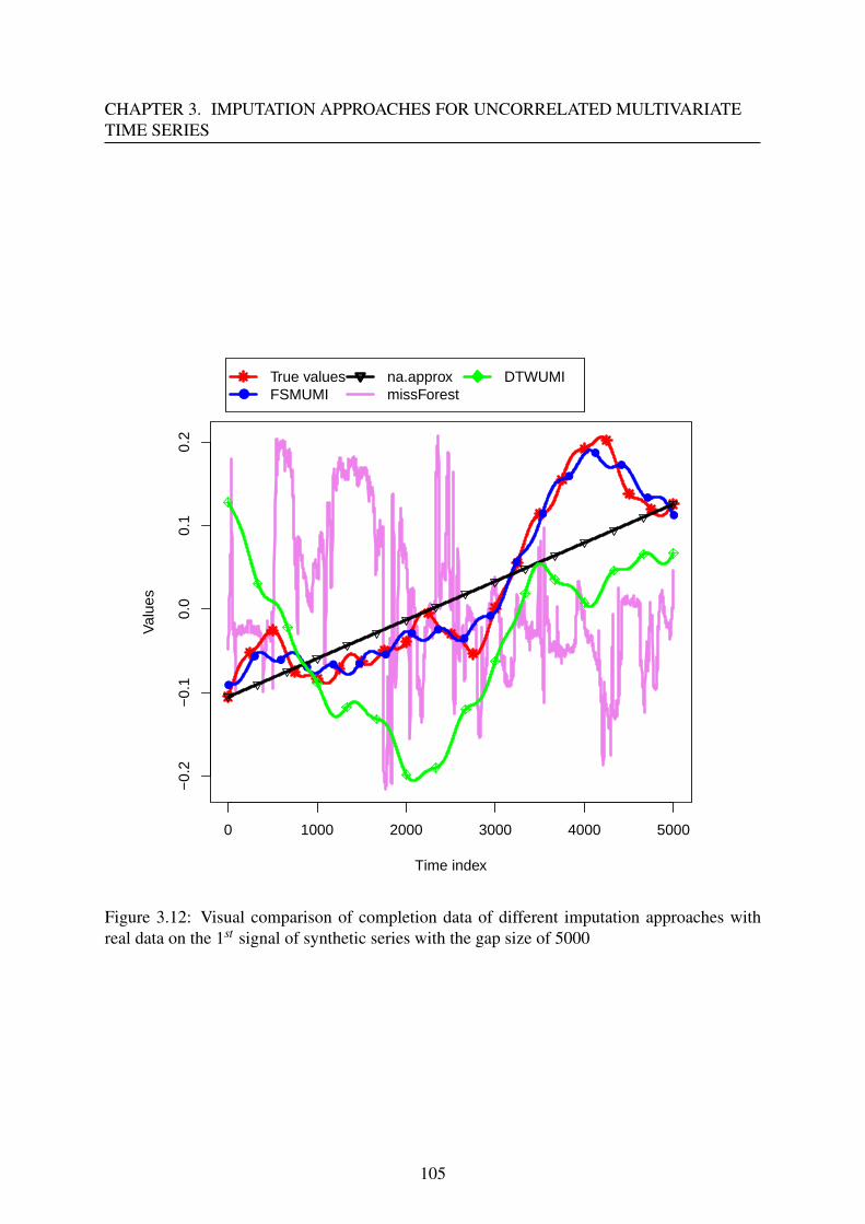
CHAPTER 3. IMPUTATION APPROACHES FOR UNCORRELATED MULTIVARIATETIME SERIES
0 1000 2000 3000 4000 5000
−0.
2−
0.1
0.0
0.1
0.2
Time index
Val
ues
●
● ●● ● ●
●
● ●●
●
●
●
●
●
●
●
●
●
True valuesFSMUMI
na.approxmissForest
DTWUMI
Figure 3.12: Visual comparison of completion data of different imputation approaches withreal data on the 1st signal of synthetic series with the gap size of 5000
105
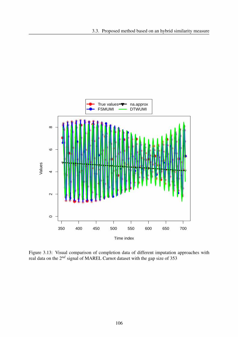
3.3. Proposed method based on an hybrid similarity measure
350 400 450 500 550 600 650 700
02
46
8
Time index
Val
ues
●
●
●
●
●
●
●
●
●
●
●●
●
●
●
●
●
●
●
True valuesFSMUMI
na.approxDTWUMI
Figure 3.13: Visual comparison of completion data of different imputation approaches withreal data on the 2nd signal of MAREL Carnot dataset with the gap size of 353
106
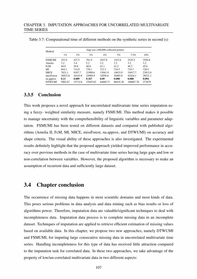
CHAPTER 3. IMPUTATION APPROACHES FOR UNCORRELATED MULTIVARIATETIME SERIES
Table 3.7: Computational time of different methods on the synthetic series in second (s)
Method Gap size (100,000 collected points)
1% 2% 3% 4% 5% 7.5% 10%
FSMUMI 353.9 427.5 701.9 1037.8 1423.6 2525.5 3556.8Amelia 3.2 3.4 5.2 3.2 3.2 3.2 3.2FcM 40.9 39.8 40.0 41.1 41.2 46.7 45.6MI 844.1 714.0 739.1 723.3 724.5 719.7 726.5MICE 7021.1 9187.7 21909.6 13041.9 14833.9 19417.7 23812.6missForest 26833.8 24143.8 22969.9 32056.6 36485.8 42424.1 28521.1na.approx 0.11 0.089 0.167 0.09 0.088 0.088 0.094DTWUMI 5002.67 15714.8 37645.82 64669.71 86435.38 180887.78 273879
3.3.5 Conclusion
This work proposes a novel approach for uncorrelated multivariate time series imputation us-
ing a fuzzy- weighted similarity measure, namely FSMUMI. This method makes it possible
to manage uncertainty with the comprehensibility of linguistic variables and parameter adap-
tation. FSMUMI has been tested on different datasets and compared with published algo-
rithms (Amelia II, FcM, MI, MICE, missForest, na.approx, and DTWUMI) on accuracy and
shape criteria. The visual ability of these approaches is also investigated. The experimental
results definitely highlight that the proposed approach yielded improved performance in accu-
racy over previous methods in the case of multivariate time series having large gaps and low or
non-correlation between variables. However, the proposed algorithm is necessary to make an
assumption of recurrent data and sufficiently large dataset.
3.4 Chapter conclusion
The occurrence of missing data happens in most scientific domains and most kinds of data.
This poses serious problems in data analysis and data mining such as bias results or loss of
algorithms power. Therefore, imputation data are valuable/significant techniques to deal with
incompleteness data. Imputation data process is to complete missing data in an incomplete
dataset. Techniques of imputation are applied to retrieve efficient estimation of missing values
based on available data. In this chapter, we propose two new approaches, namely DTWUMI
and FSMUMI, for imputing large consecutive missing data in uncorrelated multivariate time
series. Handling incompleteness for this type of data has received little attraction compared
to the imputation task for correlated data. In these two approaches, we take advantage of the
property of low/un-correlated multivariate data in two different aspects:
107
3.4. Chapter conclusion
DTWUMI is an extension of our previous proposal (DTWBI). This approach is based on
combining DTW and shape-feature extraction algorithms. To conserve time indices of all the
variables in the dataset, only one query Q is built by taking into account all the signals either
before or after each gap. DTWUMI thereafter finds the most similar window to the query using
DTW cost as the similarity criterion. This approach applies shape-feature extraction method to
decrease the computation time before using DTW algorithm to retrieve similar windows. Since
data are low/uncorrelated, so imputation data are the vector following or preceding of the most
similar window on the signal containing considered gap. In the DTWUMI, we take care of the
same time index of all the variables by creating a query window (i.e Q is a matrix of all the
signals) either before or after the gap, and find the most similar window (a matrix) to the query.
But imputation values are only a vector in the signal having the considered gap.
In the second proposal, FSMUMI, we introduce an uncertain factor that allows to manage
a high level of uncertainty, specifically:
- Develop a new similarity measure based on weighting some usually distances by applying
fuzzy rules interpolation scheme.
- And then we use the new measure to find the most similar windows. There are some
differences between these two methods:
• Step of building query: FSMUMI builds two vector queries (instead of one query matrix
as introduced in the DTWUMI): Qb - a vector previous the considered gap and Qa- a
vector next to the gap. Accordingly, we create two search databases (i) Db - a database
before the gap and (ii) Da - a database after the gap on the signal having the gap. And
we find similar windows on these two databases.
• Step of filling missing data: The final imputation data are the average of two vectors
preceding and following of the most two similar windows.
The two proposed methods are mainly compared with state-of-the-art imputation approaches
and comparisons are made in terms of accuracy and shape indices between real data and com-
pletion data. Also, the visual performance of these approaches is also investigated. DTWUMI
is compared with missForest, MI, MICE and na.approx methods on NNGC, simulated and
MAREL Carnot datasets. Whereas FSMUMI was compared with 6 well-known methods (MI,
MICE, missForest, na.approx, Amelia, FCM) and with DTWUMI on simulated dataset, syn-
thetic dataset and MAREL Carnot dataset.
108
CHAPTER 3. IMPUTATION APPROACHES FOR UNCORRELATED MULTIVARIATETIME SERIES
The experimental results clearly show that our approaches yielded improved performance
in accuracy than previous methods in the case of multivariate time series having large gaps and
low or non-correlation between variables. However, the proposed algorithms are necessary to
make an assumption of recurrent data and sufficient large dataset.
The present works open a broad range of applications, we plan to (i) combine FSMUMI/
DTWUMI method with other algorithms such as Random Forest or Deep learning in order
to efficiently fill incomplete data in any type of multivariate time series; (ii) investigate this
approach applied to short-term/long-term forecasts in multivariate time series. We could also
investigate type-2 fuzzy sets (T2FSs) [112] that are an extension of the ordinary fuzzy set (also
called type-1 fuzzy sets, T1FS). Type-2 fuzzy set can handle more uncertainty because their
membership functions are fuzzy. It is completely described by two functions (primary and
secondary fuzzy grades). Further, collected data usually contain noise (real data plus noise).
So that T2FS ([113]) should be considered to solve missing data problems in both types of
time series: univariate and multivariate time series using a new similarity measure [114] for
example. In case of bi-variate time series with small dataset, complex fuzzy sets ([113]) can be
studied instead of ordinary FSs that have given good results using an adaptive scheme.
List of Publications and valuations related to this chapter
1. Thi-Thu-Hong Phan, André Bigand, Emilie Poisson Caillault, "A New Fuzzy Logic-
based Similarity Measure applied to Large Gap Imputation for Uncorrelated Multivariate
Time Series", Applied Computational Intelligence and Soft Computing. Available online
August 2018. DOI: 10.1155/2018/9095683
2. Emilie Poisson Caillault, Camille Dezecache, Thi Thu Hong Phan, Kelly Grassi, Jean
Prygiel, and Alain Lefebvre, "Data completion, characterization of environmental states
and dynamics using multiparameter time series: DTWBI, DTWUMI and uHMM R-
packages", 2nd General Assembly of JERICO-NEXT, Galway, Ireland, 24-27 Septem-
ber, 2018.
3. Thi-Thu-Hong Phan, Emilie Poisson Caillault, Alain Lefebvre, André Bigand, "Multi-
variate times series imputation by unsupervised and supervised approach", journée IA
LISIC, 18/06/2018, Calais, France.
4. Thi-Thu-Hong Phan, Emilie Poisson Caillault, Alain Lefebvre, André Bigand, "DTW-
109

3.4. Chapter conclusion
Approach For Uncorrelated Multivariate Time Series Imputation", IEEE International
Workshop on Machine Learning for Signal Processing. MLSP 2017. September 25-28,
2017 Roppongi, Tokyo, Japan. DOI: 10.1109/MLSP.2017.8168165
5. Thi-Thu-Hong Phan, Emilie Poisson Caillault, Alain Lefebvre, André Bigand. DTW-
Approach For Uncorrelated Multivariate Time Series Imputation, 5th édition de la Journée
Doctorale du Campus de la Mer, 19 October, 2017 Boulogne sur Mer, France.
6. DTWUMI R-package https://cran.r-project.org/web/packages/DTWUMI/index.html
110
Chapter 4Applications: Toward classification and
forecasting
Contents4.1 Classification of phytoplankton species . . . . . . . . . . . . . . . . . . . 112
4.1.1 Introduction . . . . . . . . . . . . . . . . . . . . . . . . . . . . . . . 112
4.1.2 Feature-extraction algorithm . . . . . . . . . . . . . . . . . . . . . . 115
4.1.3 Methodology . . . . . . . . . . . . . . . . . . . . . . . . . . . . . . 116
4.1.4 Experiment and discussion . . . . . . . . . . . . . . . . . . . . . . . 121
4.1.5 Conclusion . . . . . . . . . . . . . . . . . . . . . . . . . . . . . . . 125
4.2 Event detection in a multidimensional time series . . . . . . . . . . . . . 125
4.2.1 Data presentation . . . . . . . . . . . . . . . . . . . . . . . . . . . . 126
4.2.2 Preprocessing data . . . . . . . . . . . . . . . . . . . . . . . . . . . 129
4.2.3 Event detection . . . . . . . . . . . . . . . . . . . . . . . . . . . . . 132
4.2.4 Conclusion . . . . . . . . . . . . . . . . . . . . . . . . . . . . . . . 134
4.3 Comparative Study on Univariate Forecasting Methods for Meteorolog-ical Time Series . . . . . . . . . . . . . . . . . . . . . . . . . . . . . . . . 136
4.3.1 Introduction . . . . . . . . . . . . . . . . . . . . . . . . . . . . . . . 136
4.3.2 Time series forecasting methods . . . . . . . . . . . . . . . . . . . . 138
4.3.3 Experiment protocol . . . . . . . . . . . . . . . . . . . . . . . . . . 140
4.3.4 Results and discussion . . . . . . . . . . . . . . . . . . . . . . . . . 141
4.3.5 Conclusion . . . . . . . . . . . . . . . . . . . . . . . . . . . . . . . 145
4.4 Chapter conclusion . . . . . . . . . . . . . . . . . . . . . . . . . . . . . . 146
111
4.1. Classification of phytoplankton species
The two previous chapters explained how to complete large consecutive missing values in
univariate time series and in uncorrelated multivariate time series. This chapter illustrates some
concrete applications in relation to the marine focus and projects (CPER MARCO project in
France and other projects in Vietnam). We begin the chapter by introducing our proposal
(section 4.1), shape-feature extraction algorithm, which allows to effectively extract global
features from a signal. Accordingly, to analyze pertinent of proposed algorithm we apply it
to classify phytoplankton species. This proposed algorithm is already combined with DTWBI
(Chapter 2) and DTWUMI (Chapter 3) in order to reduce computation time. In next sections,
we present two other applications where DTWBI is applied. In the first application, DTWBI
is employed to complete MAREL Carnot dataset, then we perform a detection of rare/extreme
events (section 4.2). In the second application (section 4.3), based on the idea of imputation,
we use DTWBI to forecast meteorological univariate time series.
4.1 Classification of phytoplankton species
Phytoplankton plays an important role in marine ecosystem. It is defined as a biological factor
to assess marine quality. The identification of phytoplankton species has a high potential for
monitoring environmental, climate changes and for evaluating water quality. However, phyto-
plankton species identification is not an easy task owing to their variability and ambiguity due
to thousands of micro and pico-plankton species. Therefore, the aim of this part is to build
a framework for identifying phytoplankton species and to perform a comparison on different
features types and classifiers. We propose a new type of features extracted from raw signals of
phytoplankton species in section 4.1.2. Then, in section 4.1.4 we analyze the performance of
various classifiers on the proposed features type as well as two other features types for finding
the most robust one.
4.1.1 Introduction
Phytoplankton is an important factor in environmental, economic and ecological policies. Be-
ing main producer of oxygen, phytoplankton is also an important food item in both aquaculture
as well as mariculture. A question is raising: “how do changes in the global environment af-
fect abundance, diversity, and production of plankton and nekton?” [115]. Many researchers
show that environment changes strongly affect to phytoplankton and that it responds promptly
112
CHAPTER 4. APPLICATIONS: TOWARD CLASSIFICATION AND FORECASTING
to chemical perturbation [116, 117, 118, 119, 120, 121]. The identification/classification of
microscopic phytoplankton is therefore crucial for a wide variety of environmental monitor-
ing applications in different domains such as: ecology (biodiversity), climate and economy. It
is thus necessary to have a capable technique/tool which can provide detailed description of
phytoplankton species population from water samples.
Up to now, studies in identification/classification of phytoplankton species are usually car-
ried out by visual comparing the collected profiles with references ones, or by the microscope
method [122, 123]. Using this microscope analysis method takes 3 to 4 hours for each sample
(low frequency). It is laborious and extremely time-consuming. Hence, developing an auto-
matic computer-aided machine system to identify/classify phytoplankton species is a required
task.
Flow cytometry (FCM) analysis is a well-known and proven tool in aquatic ecology to
quickly detect and quantify phytoplankton and bacteria (microorganism) from water samples
[124, 125]. “The various light scatter, diffraction, and fluorescence parameters measured by
analytic FCM can provide characteristic “signatures” for each microbial cell, which allow taxa
to be discriminated with the use of pattern-recognition techniques” [126]. Thus, the task of
identifying phytoplankton species becomes the classification of multidimensional signals [50].
Regarding pattern-recognition techniques, a number of successful approaches have been
proposed for automated identification/classification of plankton species.
Concerning zooplankton identification/classification, several techniques including object
classification technique for analyzing plankton images were developed by Hu and Davis [127]
and Davis et al.[128]. In these two works, the images were collected from a plankton video
recorder. A Support Vector Machine (SVM) is used for classifying a big image set (20,000
plankton images); the accuracy of classification on seven classes was achieved with the score of
71%. The performance of six classifiers: Multi-Layer Perceptron (MLP), K-Nearest Neighbors
(5-NN), SVM (using linear and Radial Basis Function (RBF) kernels), Random Forest (RF),
and C4.5 Decision Trees (DTs) were studied for classifying zooplankton images obtained from
the ZooScan system [129]. In this study, RF demonstrates the best performance and was fol-
lowed by SVM using the linear kernel. Irigoien et al. [130] carried out a research on classifying
in zooplankton images with 17 categories and RF gives the highest result. The ZooScan digital
imaging system for automatic analysis of zooplankton images is built by Grosjean et al. [115].
They tested individual classification algorithms as well as combinations of two or more dif-
ferent algorithms such as: double bagging associated with linear discriminant analysis, k-NN
113
4.1. Classification of phytoplankton species
with discriminant vector forest and specifically mix of linear discriminant analysis with learn-
ing vector quantization, and random forest. Accuracy of the last combination achieves around
75% in the task of categorizing 29 zooplankton species. In the work of classifying binary zoo-
plankton images, Luo et al. [131] investigated the performance of some classifiers, namely:
SVM, RF, C4.5 DTs, and the cascade correlation neural network. SVM proves the highest
classification performance with 90% and 75% on the six and seven classes, respectively.
Concerning phytoplankton species identification/ classification, many classification algo-
rithms were used for this task such as Artificial Neural Networks (ANNs) using FCM data
[132, 133, 134, 135, 136, 137] (72 phytoplankton species have been successfully identified by
ANN [134]). In another work, several methods namely: DTs, Naive Bayes (NB), ridge Lin-
ear Regression (LR), k-NN, SVM, bagged and boosted ensembles were applied to categorize
phytoplankton images with 12 classes and an unknown class [138]. A system using SVM clas-
sifier for automated taxonomic classification of phytoplankton sampled with imaging-in-flow-
cytometry is developed by Sosik and Olson [139]. In the work of Blaschko et al. [140], the
accuracy of two modelling approaches for predicting boreal lake phytoplankton assemblages
and their ability to detect human impact were studied. They used random forest to predict
biological group membership and species. Verikas et al. [141] have recently investigated to
detect, recognize, and estimate abundance objects representing the P.minimum species in phy-
toplankton images. The classification performance of SVM and RF methods was compared on
158 phytoplankton images.
It is found that the number of studies using plankton signals (FCM data) is less than the ones
using plankton images. Most of studies based on signals used available features generated from
a FCM system. However, only a few earlier studies used FCM signals (both available features
and raw signals) to compare the performance of classification methods [50]. In addition, RF has
proved its performance in many applications of plankton species identification/classification
[115, 129, 130, 140]. With the best of our knowledge, there is no application that combines the
FCM signals and RF to determine phytoplankton species.
Therefore, our main contributions in this part are: (1) to propose a new type of features
extracted from the raw signals of phytoplankton species; (2) to perform a comparative analysis
of identifying phytoplankton species using a variety of advance machine learning models such
as K-NN (1-NN), SVM, RF and several modification versions of RF. This permits to determine
the best type of features for representing phytoplankton species and classifier for classifying
phytoplankton species with high accuracy.
114

CHAPTER 4. APPLICATIONS: TOWARD CLASSIFICATION AND FORECASTING
4.1.2 Feature-extraction algorithm
The idea of our proposal is to propose some features that can better represent dynamics and
shape of signals. Among of the possible features, signal moments and entropy give improved
results. Denoted x = {xi|i = 1,2, · · · ,N} are the values of each signal (curve). With each raw
signal, 9 elements are calculated as follows:
• Percentile: The perth percentile of x’s values is the value that cuts off the first per percent
of x’s values when these values are sorted in ascending order (per = 30 is used in this
study).
• Max: It is the maximum of x’s values:
max(x) = max{x1,x2, . . . ,xN} (4.1)
• First moment: It is the mean of x’s values:
x = mean(x) =∑
Ni=1 xi
N(4.2)
• Standard derivation: It is the standard derivation of x’s values, based on the 2nd moment
central:
ST D(x) =
√1N
N
∑i=1
(xi− x)2 =√
µ2 (4.3)
• Median: The median of x’s values is the value separating the higher half and the lower
half. It is the middle number when the data is sorted from lowest value to highest value.
• Third moment: It is the 3rd moment of x’s values:
γ1 =µ3
µ3/22
(4.4)
where µ2 and µ3 are the second and third central moments. γ1 = 1 is the normalized 3rd
moment central (Skewness coefficient). We can know the data distribution thanks to this
coefficient.
• Nop: It is the number of peaks of x’s values calculated from the second derivative.
• Length: It is the length of the curve.
115
4.1. Classification of phytoplankton species
• Entropy: It is based on the Shannon entropy formula:
entropy(x) = −N
∑i=1
pilog(pi) (4.5)
with pi is the probability of xi
Consequently, for each signal, a features vector of dimension 9 is extracted.
4.1.3 Methodology
4.1.3.1 Data presentation
In this study, we reuse the data of the previous study [50] (Data presentation and Signal acqui-
sition). The data is acquired from 7 culture samples, whose particles belong to 7 distinct phyto-
plankton species: Chaetoceros socialis, Emiliania Huxleyi, Lauderia annulata, Leptocylindrus
minimus, Phaeocystis globosa, Skeletonema costatum and Thalassiosira rotula. Each species
is equally represented by 100 shape-profiles and each culture sample was labeled by biologists
using a microscope [123]. So, the data set has 700 (100×7) phytoplankton cells.
Signal acquisition
Multi-signals were gathered in the LOG laboratory1 from different phytoplankton species
living in Eastern Channel, with a CytoSense flow cytometer (CytoBuoy2), and labeled by bi-
ologists [123] once having them isolated from the natural environment. Flow cytometry is a
technique used to characterize individual particles (cells or bacteria) derived by a liquid flow
at high speed in front of a laser light. Different signals either optical or physical are provided:
forward scatter (reflecting the particle length), sideward scatter (being more dependent on the
particle internal structure) and several wavelengths of fluorescence that depend upon the type
of its photosynthetic pigments measures.
More precisely, in the used signal library, each detected particle is described by 8 mono-
dimensional raw signals issued from the flow cytometer in identical experimental conditions
(same sampling rates, same detection threshold, etc.):
• one signal on forward scatter (FWS), corresponding to the cell length;
• two signals on sideward scatter (SWS), corresponding to the internal structure, in high
and low sensitivity levels (SWS HS, SWS LS);1Laboratoire d’Oceanologie et de Géosciences, UMR 8187: http://log.univ-littoral.fr2Cytobuoy system: http://www.cytobuoy.com
116
CHAPTER 4. APPLICATIONS: TOWARD CLASSIFICATION AND FORECASTING
• two signals on red fluorescence (FLR), λem > 620nm in high and low sensitivity (FLR
HS, FLR LS), which characterize chlorophyll pigments;
• one signal on orange fluorescence (FLO), 565nm < λem < 592nm, in low sensitivity
(FLO LS);
• two signals on yellow fluorescence (FLY), 545nm < λem < 570nm, in high and low
sensitivity (FLY HS, FLY LS).
These signals are composed of voltage measures (µV), and their sampling period was here
chosen to correspond to 0.5 µm displacement of the water flow. Consequently, the longer the
cell is, the higher the number of sampled measures is, and the time axis can be interpreted as
a spatial length axis. Phytoplankton species identification is a hard task so all these signals are
used to make the particles characterization. Each particle of our experiment is consequently
characterized by the 8 signals described above. Figure 4.1 present some signal samples of
Chaetoceros socialis, Lauderia annulata and Skeletonema costatum species.
4.1.3.2 Phytoplankton descriptor
After acquiring phytoplankton raw signals from the FCM system, phytoplankton descriptor
must be computed to represent the phytoplankton species, that will be presented to a classifier.
The phytoplankton descriptor describes properties of a phytoplankton cell (for example length,
number of peaks . . . of each raw signal or the ratio of dissimilarity of each pairs of phytoplank-
ton cells). In this work, these properties are typically called “features”. We investigate three
types of features : derived features, proposed features (as above mentioned) and dissimilarity
features [50].
1. Derived features
For each signal, 4 elements are extracted by a Cytobuoy machine including: length,
height, integral, and number of peaks. So each phytoplankton cell is represented by a
vector of 32 features.
2. Proposed features
As mentioned above in our proposal, 9 characteristics will be extracted from each signal.
However, when applying to the phytoplankton classification, we have modified some
features to adapt the data in the following:
117
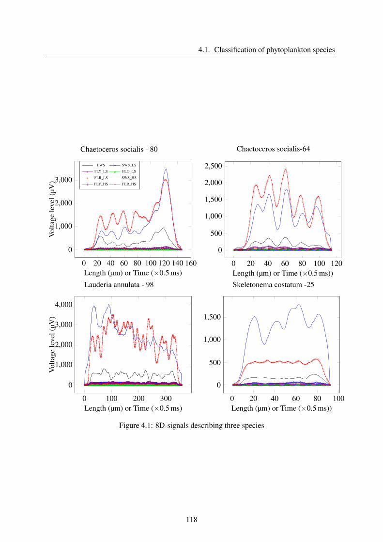
4.1. Classification of phytoplankton species
Chaetoceros socialis - 80
0 20 40 60 80 100 120 140 160
0
1,000
2,000
3,000
Length (µm) or Time (×0.5 ms)
Volta
gele
vel(
µV)
FWS SWS_LS
FLY_LS FLO_LS
FLR_LS SWS_HS
FLY_HS FLR_HS
Chaetoceros socialis-64
0 20 40 60 80 100 120
0
500
1,000
1,500
2,000
2,500
Length (µm) or Time (×0.5 ms))Lauderia annulata - 98
0 100 200 300
0
1,000
2,000
3,000
4,000
Length (µm) or Time (×0.5 ms)
Volta
gele
vel(
µV)
Skeletonema costatum -25
0 20 40 60 80 100
0
500
1,000
1,500
Length (µm) or Time (×0.5 ms))
Figure 4.1: 8D-signals describing three species
118
CHAPTER 4. APPLICATIONS: TOWARD CLASSIFICATION AND FORECASTING
• Third moment: we use the 3rd moment instead of utilizing the Skewness coefficient
because some signals have all 0 values.
• Entropy: With this application pi is computed as follows: pi =xi
∑Ni=1 xi
because we
could exploit all the values of each signal.
For each signal 9 features are extracted. Consequently, the proposed features vector
is 72 dimensions.
3. Dissimilarity features
As described in Chapter 2, Dynamic Time Warping [7] is an algorithm devoted to align
two sequences (may vary in time) by warping the time axis until finding an optimal
matching between the two sequences according to suitable metrics. However, it is not
easy to interpret the matching cost. Thus, Caillaut et al. [50] proposed a dissimilarity
distance that adapts the DTW matching cost and can deal with multidimensional signals.
They replaced the distance d (L1–distance or L2–distance) by a dissimilarity s (s ∈ [0,1]-
normalized dissimilarity degree):
s(xil ,y jl ) =d(xil ,y jl )
max{d(xil ,0),d(y jl ,0)}(4.6)
where x = {x1,x2, . . . ,xN} and y = {y1,y2, . . . ,yM} are two signals of different size. The
algorithm makes a matching P = {(il , jl), l = 1 . . .k, il = 1 . . .N, jl = 1 . . .M} between
the points of x and y signals, according to some time conditions.
Therefore, each phytoplankton cell is presented by a vector of 700 dissimilarity features,
in which a feature is the DTW dissimilarity between considered cell and one cell in the
dataset.
4.1.3.3 Classification
After feature extraction, a classifier is learned for identification of different phytoplankton
species. In the following, we review several prominent classification models:
1. k-Nearest Neighbors
k-nearest neighbors [142] has been widely used in classification problems because it is
simple, effective and nonparametric [143]. For each sample of a test set, we found k
cases in the train set that is minimum distance between the feature vectors of the sample
119
4.1. Classification of phytoplankton species
and those of the train set. A decision of the label of a new sample is based on majority
vote of the k label found.
2. Support Vector Machine
The basic idea of support vector machine [144] is to find an optimal hyper-plane for
linearly separable patterns in a high dimensional space where features are mapped onto.
The work is to detect the one that maximizes the margin around the separating hyper-
plane from training set. A decision on the label of a new sample is based on its distance
with the trained support vectors.
3. Random Forest
Breiman [145] proposed random forest, a classification technique obtained by construct-
ing an ensemble of decision trees, in which each decision tree uses a different bootstrap
sample of the response variables and at each node, a small subset of randomly selected
variables from original ones for the binary splitting. For predicting new data, a RF ag-
gregates the outputs of all trees.
4. Regularized Random Forest (RRF), Guided RRF (GRRF), Guided RF (GRF)
RRF, GRRF, GRF are different modified versions of the original RF. But these methods
are just similar to initial RF method in the step of predicting new data, and they are
different in step of finding features to build each decision tree of forest. Indeed, RRF
was proposed for improving feature selection on the decision tree by limiting the choice
of new feature at each tree node and evaluating features (using Gini index) on a part of
the training data [146]. This process of feature selection is greedy because variables are
selected based on a subsample of data variables at each node.
GRRF [147] is an enhanced RRF. This approach uses the feature importance scores gen-
erated from an initial random forest to guide the feature selection process in RRF for
avoiding of selecting not strongly relevant features. While GRRF selects a subset of rel-
evant and non-redundant features, GRF selects a subset of “relevant” features. So GRF
often selects a lot more features than GRRF (sometimes most of the features), but it
may lead to better classification accuracy than GRRF. Nevertheless, each tree of GRF is
built independently and GRF can be implemented in a distributed computing framework
[148].
120
CHAPTER 4. APPLICATIONS: TOWARD CLASSIFICATION AND FORECASTING
4.1.4 Experiment and discussion
We have conducted a set of experiments on various types of features and classification models
to evaluate their performance on phytoplankton species data (as mentioned above).
Experimental set up
To conduct all experiments, we use a computer with 64 bits Window 7, core i7, CPU 3.0
GHz and 8 GB main memory. For computing the proposed features we use the following R-
packages: base, stats, moment [149], and entropy [150]. We utilize the latest R-packages of RF
[145], RRF (RRF, GRRF, and GRF)[151], e1071 package (SVM) [152], class package (k-NN)
[153] for classifying. Other R-packages like FactoMineR [154], lda [155], have been used to
find the most important features.
Concerning SVM, after testing different kernels on different types of features, we choose
polynomial kernel of SVM (degree =3) for the derived features and the dissimilarity features,
RBF kernel of SVM for the proposed features (tune.svm function [152] is used to find out the
optimal coefficients (γ = 0.01 and C = 32, for example)). With k-NN, one of the most important
parameters is to choice of suitable value of K. In our experiment, we test with different values
of k (k = 1 to 10) and this model gives the best results when k = 1.
For RF, the basic two parameters are specified to train the model are: ntree - number of
trees to be constructed in the forest and mtry - number of input variables randomly sampled as
candidates at each node. In this study, ntree = 500 is fixed for all RF versions. mtry of RF, γ
of GRRF and γ of GRF are default values: the square root of the number of features [145], 0.1
[147] and 1 [151], respectively.
Each classifier is evaluated using a 4-fold cross validation to determine the recognition error
rate and this cross validation is repeated 10 times. The data set of 700 (100×7) phytoplankton
cells is divided into 4 subsets of 175 (25 × 7) cells. Each subset respects an equal target distribu-
tion. The learning phase uses three subsets and predicts the remains as test set. For classifying
phytoplankton species, in the first step, we extract proposed features (derived features are avail-
able) and calculate dissimilarity of each pairs phytoplankton cells from the raw signals. In the
next step, after finishing of the learning process, the classification models are used to predict
test set. The average accuracy of classification methods are given in tables 4.1, 4.2, and 4.3.
The results of contingency table between different models and between different features types
of one in the 10 iterations are presented in tables 4.4, 4.5.
The reliability of classification models is evaluated based on classification accuracy of the
test sets. The classification results of six methods using different features types are illustrated
121
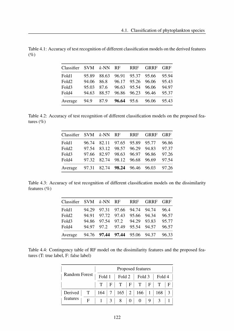
4.1. Classification of phytoplankton species
Table 4.1: Accuracy of test recognition of different classification models on the derived features(%)
Classifier SVM k-NN RF RRF GRRF GRF
Fold1 95.89 88.63 96.91 95.37 95.66 95.94Fold2 94.06 86.8 96.17 95.26 96.06 95.43Fold3 95.03 87.6 96.63 95.54 96.06 94.97Fold4 94.63 88.57 96.86 96.23 96.46 95.37
Average 94.9 87.9 96.64 95.6 96.06 95.43
Table 4.2: Accuracy of test recognition of different classification models on the proposed fea-tures (%)
Classifier SVM k-NN RF RRF GRRF GRF
Fold1 96.74 82.11 97.65 95.89 95.77 96.86Fold2 97.54 83.12 98.57 96.29 94.83 97.37Fold3 97.66 82.97 98.63 96.97 96.86 97.26Fold4 97.32 82.74 98.12 96.68 96.69 97.54
Average 97.31 82.74 98.24 96.46 96.03 97.26
Table 4.3: Accuracy of test recognition of different classification models on the dissimilarityfeatures (%)
Classifier SVM k-NN RF RRF GRRF GRF
Fold1 94.29 97.31 97.66 94.74 94.74 96.4Fold2 94.91 97.72 97.43 95.66 94.34 96.57Fold3 94.86 97.54 97.2 94.29 93.83 95.77Fold4 94.97 97.2 97.49 95.54 94.57 96.57
Average 94.76 97.44 97.44 95.06 94.37 96.33
Table 4.4: Contingency table of RF model on the dissimilarity features and the proposed fea-tures (T: true label, F: false label)
Random ForestProposed features
Fold 1 Fold 2 Fold 3 Fold 4
T F T F T F T F
Derivedfeatures
T 164 7 165 2 166 1 168 3
F 1 3 8 0 0 9 3 1
122
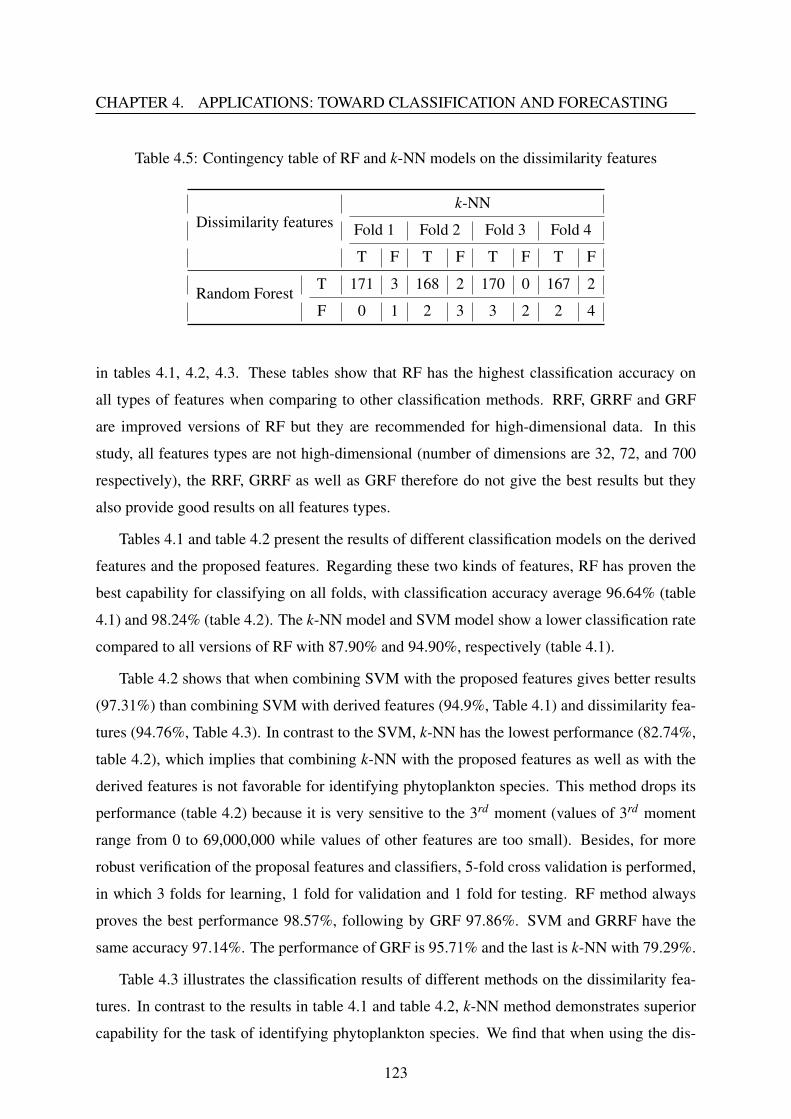
CHAPTER 4. APPLICATIONS: TOWARD CLASSIFICATION AND FORECASTING
Table 4.5: Contingency table of RF and k-NN models on the dissimilarity features
Dissimilarity featuresk-NN
Fold 1 Fold 2 Fold 3 Fold 4
T F T F T F T F
Random ForestT 171 3 168 2 170 0 167 2
F 0 1 2 3 3 2 2 4
in tables 4.1, 4.2, 4.3. These tables show that RF has the highest classification accuracy on
all types of features when comparing to other classification methods. RRF, GRRF and GRF
are improved versions of RF but they are recommended for high-dimensional data. In this
study, all features types are not high-dimensional (number of dimensions are 32, 72, and 700
respectively), the RRF, GRRF as well as GRF therefore do not give the best results but they
also provide good results on all features types.
Tables 4.1 and table 4.2 present the results of different classification models on the derived
features and the proposed features. Regarding these two kinds of features, RF has proven the
best capability for classifying on all folds, with classification accuracy average 96.64% (table
4.1) and 98.24% (table 4.2). The k-NN model and SVM model show a lower classification rate
compared to all versions of RF with 87.90% and 94.90%, respectively (table 4.1).
Table 4.2 shows that when combining SVM with the proposed features gives better results
(97.31%) than combining SVM with derived features (94.9%, Table 4.1) and dissimilarity fea-
tures (94.76%, Table 4.3). In contrast to the SVM, k-NN has the lowest performance (82.74%,
table 4.2), which implies that combining k-NN with the proposed features as well as with the
derived features is not favorable for identifying phytoplankton species. This method drops its
performance (table 4.2) because it is very sensitive to the 3rd moment (values of 3rd moment
range from 0 to 69,000,000 while values of other features are too small). Besides, for more
robust verification of the proposal features and classifiers, 5-fold cross validation is performed,
in which 3 folds for learning, 1 fold for validation and 1 fold for testing. RF method always
proves the best performance 98.57%, following by GRF 97.86%. SVM and GRRF have the
same accuracy 97.14%. The performance of GRF is 95.71% and the last is k-NN with 79.29%.
Table 4.3 illustrates the classification results of different methods on the dissimilarity fea-
tures. In contrast to the results in table 4.1 and table 4.2, k-NN method demonstrates superior
capability for the task of identifying phytoplankton species. We find that when using the dis-
123
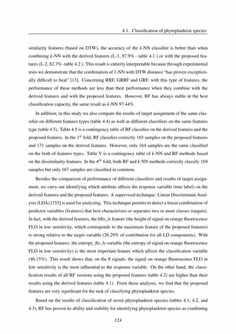
4.1. Classification of phytoplankton species
similarity features (based on DTW), the accuracy of the k-NN classifier is better than when
combining k-NN with the derived features (L-1, 87.9% - table 4.1 ) or with the proposed fea-
tures (L-2, 82.7% -table 4.2 ). This result is entirely interpretable because through experimental
tests we demonstrate that the combination of 1-NN with DTW distance “has proven exception-
ally difficult to beat” [13]. Concerning RRF, GRRF and GRF, with this type of features, the
performance of these methods are less than their performance when they combine with the
derived features and with the proposed features. However, RF has always stable in the best
classification capacity, the same result as k-NN 97.44%.
In addition, in this study we also compare the results of target assignment of the same clas-
sifier on different features types (table 4.4) as well as different classifiers on the same features
type (table 4.5). Table 4.5 is a contingency table of RF classifier on the derived features and the
proposed features. In the 1st fold, RF classifies correctly 165 samples on the proposed features
and 171 samples on the derived features. However, only 164 samples are the same classified
on the both of features types. Table V is a contingency table of k-NN and RF methods based
on the dissimilarity features. In the 4th fold, both RF and k-NN methods correctly classify 169
samples but only 167 samples are classified in common.
Besides the comparison of performance of different classifiers and results of target assign-
ment, we carry out identifying which attribute affects the response variable (true label) on the
derived features and the proposed features. A supervised technique: Linear Discriminant Anal-
ysis (LDA) [155] is used for analyzing. This technique permits to detect a linear combination of
predictor variables (features) that best characterizes or separates two or more classes (targets).
In fact, with the derived features, the hflo_ls feature (the height of signal on orange fluorescence
FLO in low sensitivity, which corresponds to the maximum feature of the proposed features)
is strong relative to the target variable (28.29% of contribution for all LD components). With
the proposed features: the entropy_flo_ls variable (the entropy of signal on orange fluorescence
FLO in low sensitivity) is the most important feature which affects the classification variable
(46.15%). This result shows that, on the 8 signals, the signal on orange fluorescence FLO in
low sensitivity is the most influential to the response variable. On the other hand, the classi-
fication results of all RF versions using the proposed features (table 4.2) are higher than their
results using the derived features (table 4.1). From these analyses, we find that the proposed
features are very significant for the task of classifying phytoplankton species.
Based on the results of classification of seven phytoplankton species (tables 4.1, 4.2, and
4.3), RF has proven its ability and stability for identifying phytoplankton species as combining
124
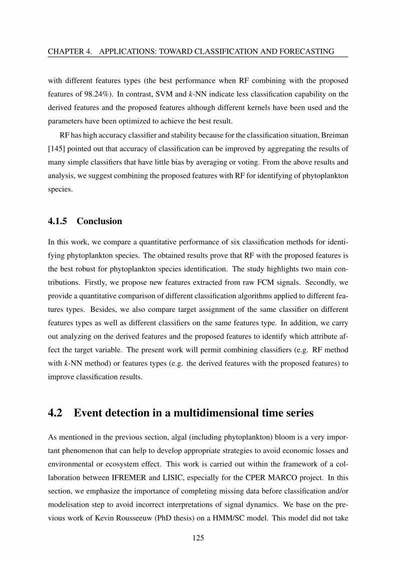
CHAPTER 4. APPLICATIONS: TOWARD CLASSIFICATION AND FORECASTING
with different features types (the best performance when RF combining with the proposed
features of 98.24%). In contrast, SVM and k-NN indicate less classification capability on the
derived features and the proposed features although different kernels have been used and the
parameters have been optimized to achieve the best result.
RF has high accuracy classifier and stability because for the classification situation, Breiman
[145] pointed out that accuracy of classification can be improved by aggregating the results of
many simple classifiers that have little bias by averaging or voting. From the above results and
analysis, we suggest combining the proposed features with RF for identifying of phytoplankton
species.
4.1.5 Conclusion
In this work, we compare a quantitative performance of six classification methods for identi-
fying phytoplankton species. The obtained results prove that RF with the proposed features is
the best robust for phytoplankton species identification. The study highlights two main con-
tributions. Firstly, we propose new features extracted from raw FCM signals. Secondly, we
provide a quantitative comparison of different classification algorithms applied to different fea-
tures types. Besides, we also compare target assignment of the same classifier on different
features types as well as different classifiers on the same features type. In addition, we carry
out analyzing on the derived features and the proposed features to identify which attribute af-
fect the target variable. The present work will permit combining classifiers (e.g. RF method
with k-NN method) or features types (e.g. the derived features with the proposed features) to
improve classification results.
4.2 Event detection in a multidimensional time series
As mentioned in the previous section, algal (including phytoplankton) bloom is a very impor-
tant phenomenon that can help to develop appropriate strategies to avoid economic losses and
environmental or ecosystem effect. This work is carried out within the framework of a col-
laboration between IFREMER and LISIC, especially for the CPER MARCO project. In this
section, we emphasize the importance of completing missing data before classification and/or
modelisation step to avoid incorrect interpretations of signal dynamics. We base on the pre-
vious work of Kevin Rousseeuw (PhD thesis) on a HMM/SC model. This model did not take
125
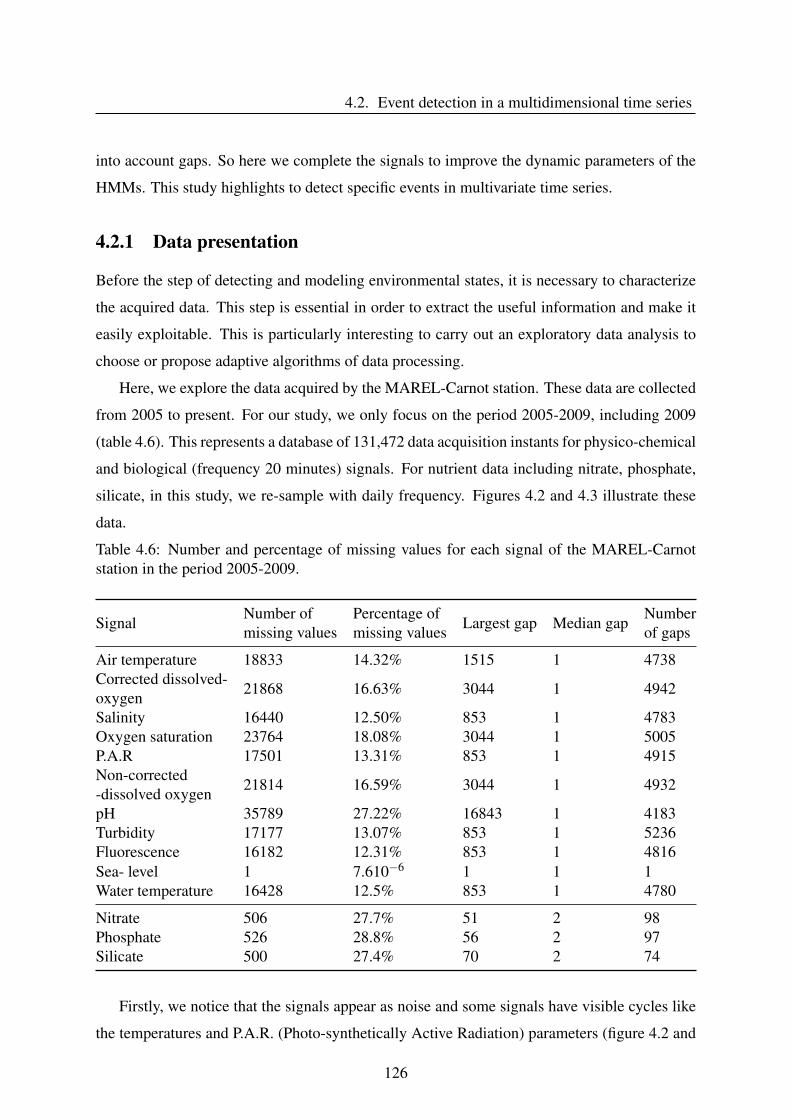
4.2. Event detection in a multidimensional time series
into account gaps. So here we complete the signals to improve the dynamic parameters of the
HMMs. This study highlights to detect specific events in multivariate time series.
4.2.1 Data presentation
Before the step of detecting and modeling environmental states, it is necessary to characterize
the acquired data. This step is essential in order to extract the useful information and make it
easily exploitable. This is particularly interesting to carry out an exploratory data analysis to
choose or propose adaptive algorithms of data processing.
Here, we explore the data acquired by the MAREL-Carnot station. These data are collected
from 2005 to present. For our study, we only focus on the period 2005-2009, including 2009
(table 4.6). This represents a database of 131,472 data acquisition instants for physico-chemical
and biological (frequency 20 minutes) signals. For nutrient data including nitrate, phosphate,
silicate, in this study, we re-sample with daily frequency. Figures 4.2 and 4.3 illustrate these
data.
Table 4.6: Number and percentage of missing values for each signal of the MAREL-Carnotstation in the period 2005-2009.
SignalNumber ofmissing values
Percentage ofmissing values Largest gap Median gap
Numberof gaps
Air temperature 18833 14.32% 1515 1 4738Corrected dissolved-oxygen 21868 16.63% 3044 1 4942
Salinity 16440 12.50% 853 1 4783Oxygen saturation 23764 18.08% 3044 1 5005P.A.R 17501 13.31% 853 1 4915Non-corrected-dissolved oxygen 21814 16.59% 3044 1 4932
pH 35789 27.22% 16843 1 4183Turbidity 17177 13.07% 853 1 5236Fluorescence 16182 12.31% 853 1 4816Sea- level 1 7.610−6 1 1 1Water temperature 16428 12.5% 853 1 4780
Nitrate 506 27.7% 51 2 98Phosphate 526 28.8% 56 2 97Silicate 500 27.4% 70 2 74
Firstly, we notice that the signals appear as noise and some signals have visible cycles like
the temperatures and P.A.R. (Photo-synthetically Active Radiation) parameters (figure 4.2 and
126
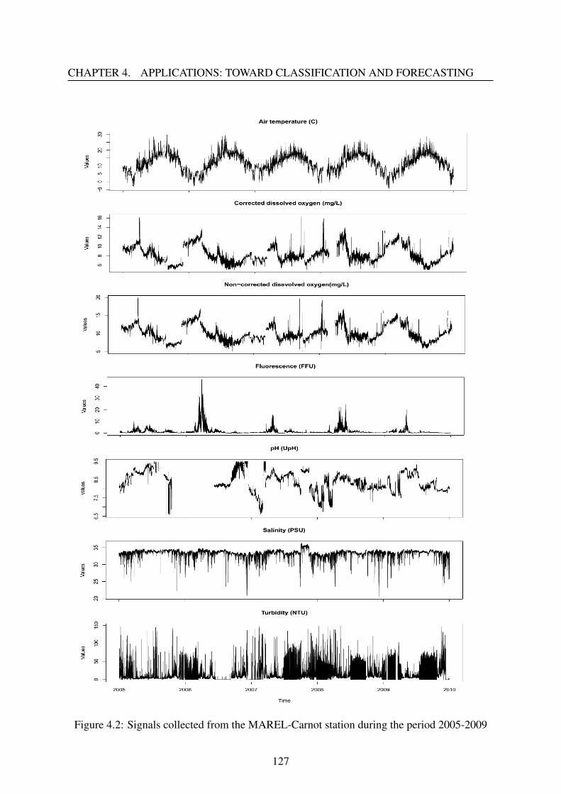
CHAPTER 4. APPLICATIONS: TOWARD CLASSIFICATION AND FORECASTING
Figure 4.2: Signals collected from the MAREL-Carnot station during the period 2005-2009
127
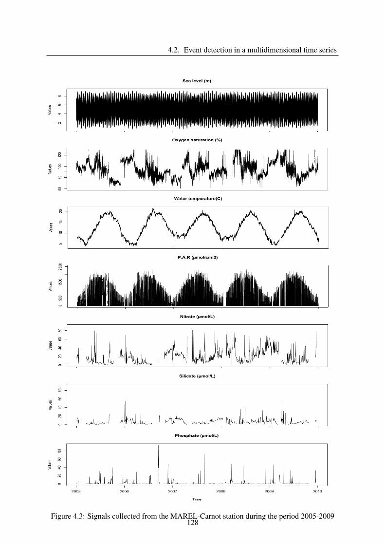
4.2. Event detection in a multidimensional time series
Figure 4.3: Signals collected from the MAREL-Carnot station during the period 2005-2009128
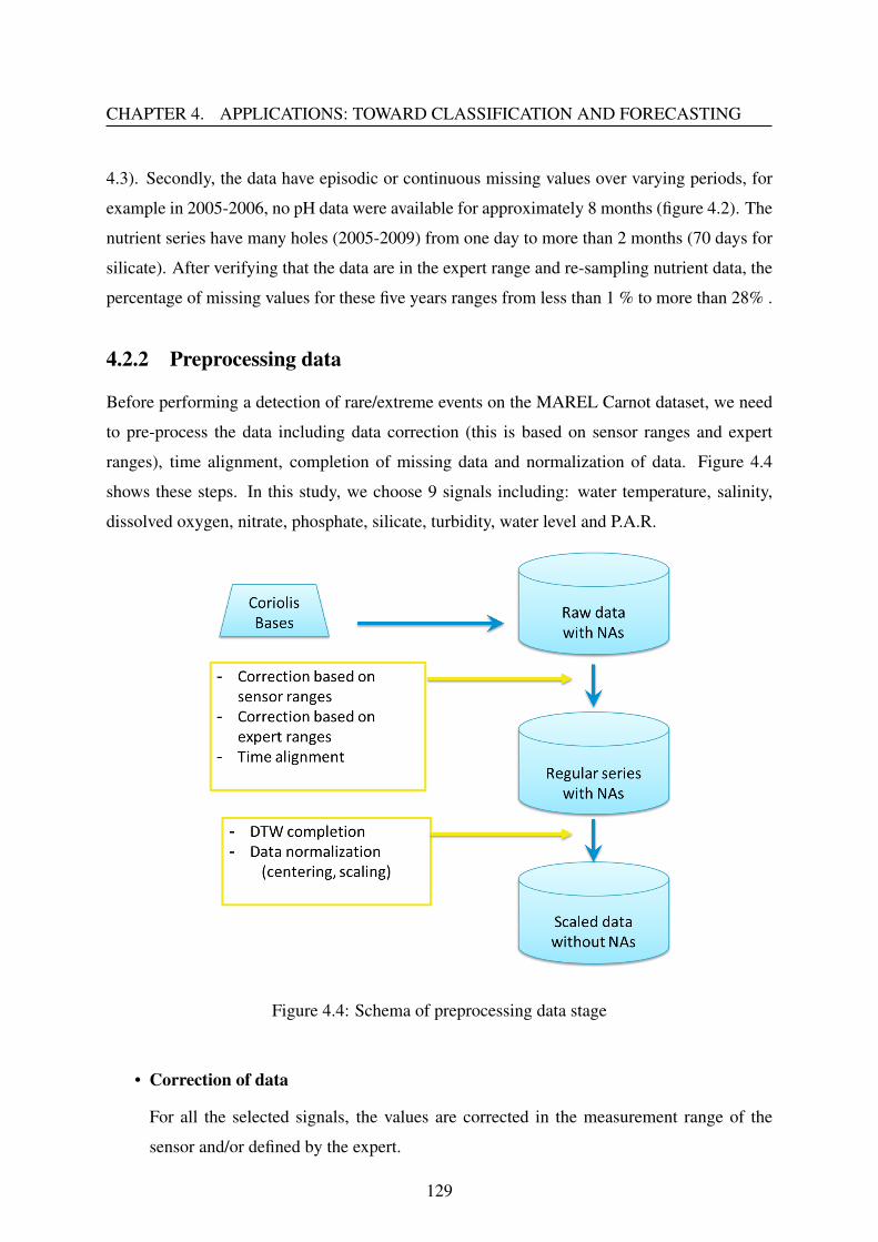
CHAPTER 4. APPLICATIONS: TOWARD CLASSIFICATION AND FORECASTING
4.3). Secondly, the data have episodic or continuous missing values over varying periods, for
example in 2005-2006, no pH data were available for approximately 8 months (figure 4.2). The
nutrient series have many holes (2005-2009) from one day to more than 2 months (70 days for
silicate). After verifying that the data are in the expert range and re-sampling nutrient data, the
percentage of missing values for these five years ranges from less than 1 % to more than 28% .
4.2.2 Preprocessing data
Before performing a detection of rare/extreme events on the MAREL Carnot dataset, we need
to pre-process the data including data correction (this is based on sensor ranges and expert
ranges), time alignment, completion of missing data and normalization of data. Figure 4.4
shows these steps. In this study, we choose 9 signals including: water temperature, salinity,
dissolved oxygen, nitrate, phosphate, silicate, turbidity, water level and P.A.R.
Figure 4.4: Schema of preprocessing data stage
• Correction of data
For all the selected signals, the values are corrected in the measurement range of the
sensor and/or defined by the expert.
129
4.2. Event detection in a multidimensional time series
• Time alignment
The acquisition frequency of MAREL-Carnot data is 20 minutes. However, the mea-
surements of various sensors are not done simultaneously, so there is a time shift that
can range from a few seconds to a few minutes. The characteristics of the seawater do
not radically change every minute, so in order to synchronize the measurements, after
deleting the information on the seconds, a time alignment with interval of 20 minutes is
performed. For each hour (noted hh), we obtain the alignment as follows:
• [ hh:00, hh:20 [ = hh:10
• [ hh:20 , hh:40 [ = hh:30
• [ hh:40 , hh:59 ] = hh:50
So the moment 01:21 will be labeled as the moment 01:30. Our database therefore con-
sists of = 131,472 times starting on 01/01/2005 at 00:10 and ending on 31/12/2009 at
23:50 with a sampling time of 20 minutes. For nutrients with a lower frequency (12
hours), we re-sample with daily frequency.
• Completion of missing data
As mentioned above, MAREL Carnot data contain a lot of missing values. There are
many isolated missing points and gaps. We apply DTWBI to complete gaps when their
size are larger or equal to 9 missing values (corresponding to 3 hours). For isolated
missing values and gaps which are smaller than 9 missing points, we use two algorithms
as following :
1. Imputing isolated missing - 1NA: replacing a missing value by the average of the
previous value and the following one of the missing value at time index t.
2. Imputing small T-gaps (for Marel case T<=9 - corresponding to less than 3 hours):
This method is an extension of the previous one (we named Weighted Moving Av-
erage method). The difference is in the update step of the considered window. This
algorithm involves 3 steps as follows:
- Calculate weighted moving average (direction left to right) wl
- Calculate weighted moving average (direction right to left) wr
- Compute the average of wl and wr to fill in missing values
130
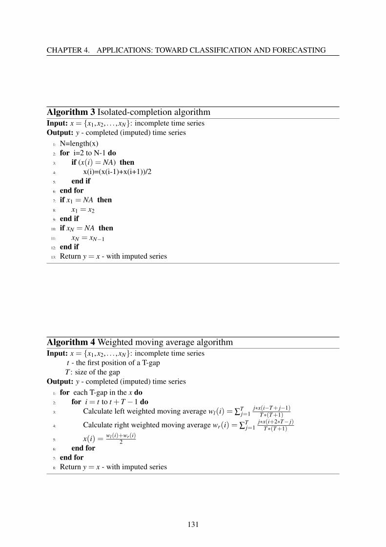
CHAPTER 4. APPLICATIONS: TOWARD CLASSIFICATION AND FORECASTING
Algorithm 3 Isolated-completion algorithmInput: x = {x1,x2, . . . ,xN}: incomplete time seriesOutput: y - completed (imputed) time series
1: N=length(x)2: for i=2 to N-1 do3: if (x(i) = NA) then4: x(i)=(x(i-1)+x(i+1))/25: end if6: end for7: if x1 = NA then8: x1 = x29: end if
10: if xN = NA then11: xN = xN−112: end if13: Return y = x - with imputed series
Algorithm 4 Weighted moving average algorithmInput: x = {x1,x2, . . . ,xN}: incomplete time series
t - the first position of a T-gapT : size of the gap
Output: y - completed (imputed) time series1: for each T-gap in the x do2: for i = t to t +T −1 do3: Calculate left weighted moving average wl(i) = ∑
Tj=1
j∗x(i−T+ j−1)T∗(T+1)
4: Calculate right weighted moving average wr(i) = ∑Tj=1
j∗x(i+2∗T− j)T∗(T+1)
5: x(i) = wl(i)+wr(i)2
6: end for7: end for8: Return y = x - with imputed series
131
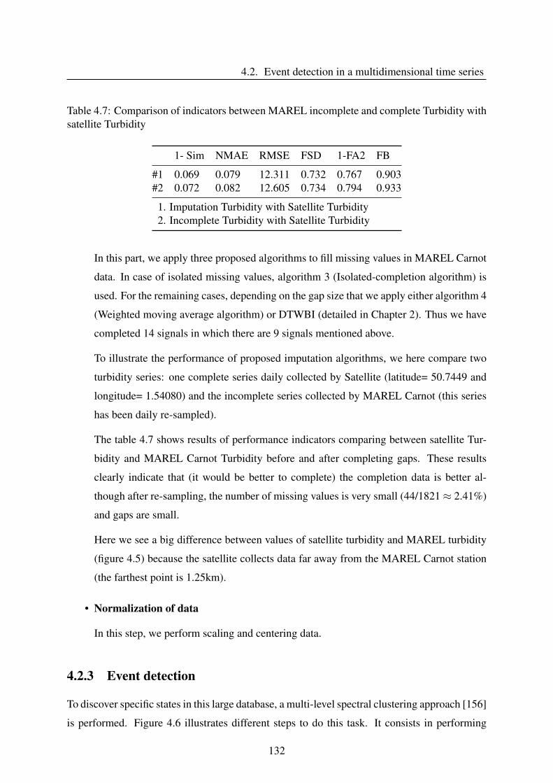
4.2. Event detection in a multidimensional time series
Table 4.7: Comparison of indicators between MAREL incomplete and complete Turbidity withsatellite Turbidity
1- Sim NMAE RMSE FSD 1-FA2 FB
#1 0.069 0.079 12.311 0.732 0.767 0.903#2 0.072 0.082 12.605 0.734 0.794 0.933
1. Imputation Turbidity with Satellite Turbidity2. Incomplete Turbidity with Satellite Turbidity
In this part, we apply three proposed algorithms to fill missing values in MAREL Carnot
data. In case of isolated missing values, algorithm 3 (Isolated-completion algorithm) is
used. For the remaining cases, depending on the gap size that we apply either algorithm 4
(Weighted moving average algorithm) or DTWBI (detailed in Chapter 2). Thus we have
completed 14 signals in which there are 9 signals mentioned above.
To illustrate the performance of proposed imputation algorithms, we here compare two
turbidity series: one complete series daily collected by Satellite (latitude= 50.7449 and
longitude= 1.54080) and the incomplete series collected by MAREL Carnot (this series
has been daily re-sampled).
The table 4.7 shows results of performance indicators comparing between satellite Tur-
bidity and MAREL Carnot Turbidity before and after completing gaps. These results
clearly indicate that (it would be better to complete) the completion data is better al-
though after re-sampling, the number of missing values is very small (44/1821≈ 2.41%)
and gaps are small.
Here we see a big difference between values of satellite turbidity and MAREL turbidity
(figure 4.5) because the satellite collects data far away from the MAREL Carnot station
(the farthest point is 1.25km).
• Normalization of data
In this step, we perform scaling and centering data.
4.2.3 Event detection
To discover specific states in this large database, a multi-level spectral clustering approach [156]
is performed. Figure 4.6 illustrates different steps to do this task. It consists in performing
132
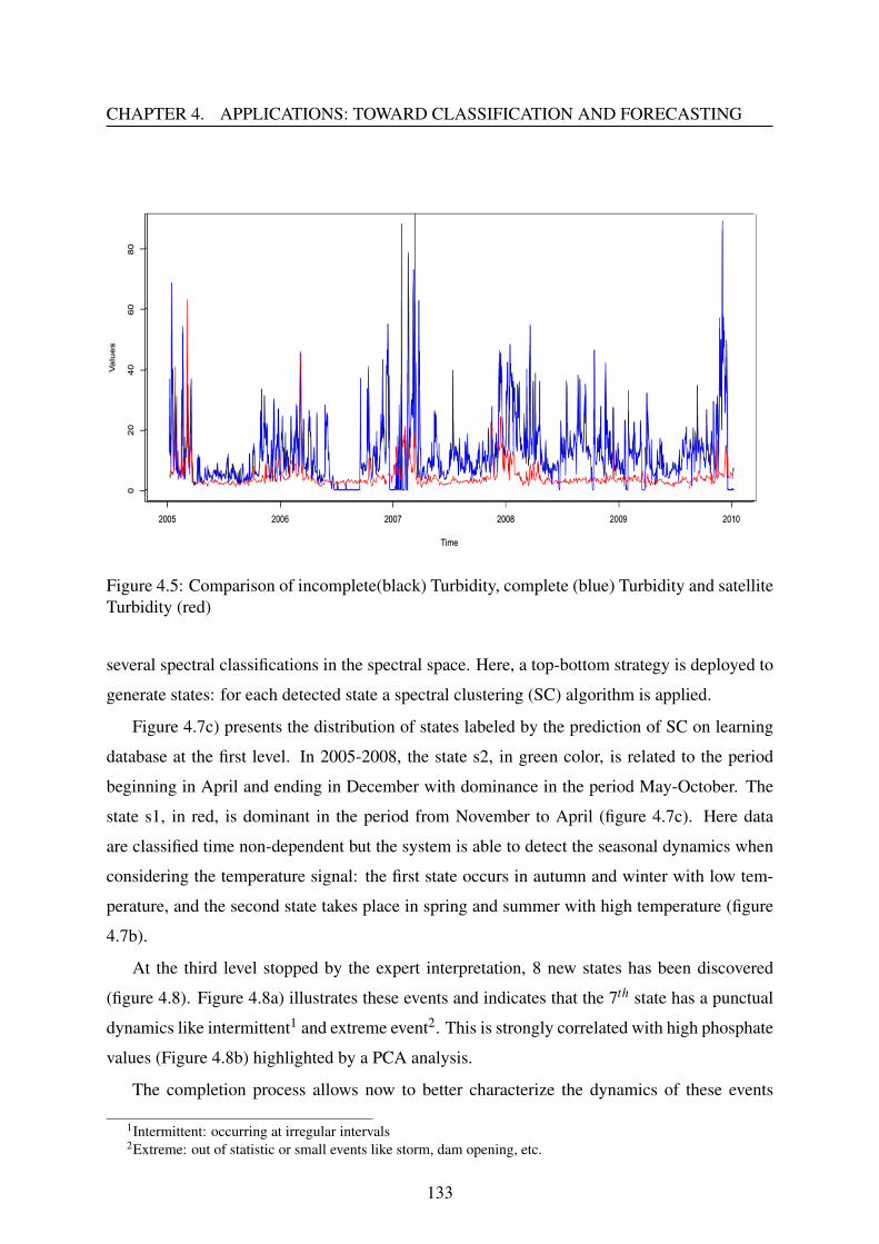
CHAPTER 4. APPLICATIONS: TOWARD CLASSIFICATION AND FORECASTING
Figure 4.5: Comparison of incomplete(black) Turbidity, complete (blue) Turbidity and satelliteTurbidity (red)
several spectral classifications in the spectral space. Here, a top-bottom strategy is deployed to
generate states: for each detected state a spectral clustering (SC) algorithm is applied.
Figure 4.7c) presents the distribution of states labeled by the prediction of SC on learning
database at the first level. In 2005-2008, the state s2, in green color, is related to the period
beginning in April and ending in December with dominance in the period May-October. The
state s1, in red, is dominant in the period from November to April (figure 4.7c). Here data
are classified time non-dependent but the system is able to detect the seasonal dynamics when
considering the temperature signal: the first state occurs in autumn and winter with low tem-
perature, and the second state takes place in spring and summer with high temperature (figure
4.7b).
At the third level stopped by the expert interpretation, 8 new states has been discovered
(figure 4.8). Figure 4.8a) illustrates these events and indicates that the 7th state has a punctual
dynamics like intermittent1 and extreme event2. This is strongly correlated with high phosphate
values (Figure 4.8b) highlighted by a PCA analysis.
The completion process allows now to better characterize the dynamics of these events
1Intermittent: occurring at irregular intervals2Extreme: out of statistic or small events like storm, dam opening, etc.
133
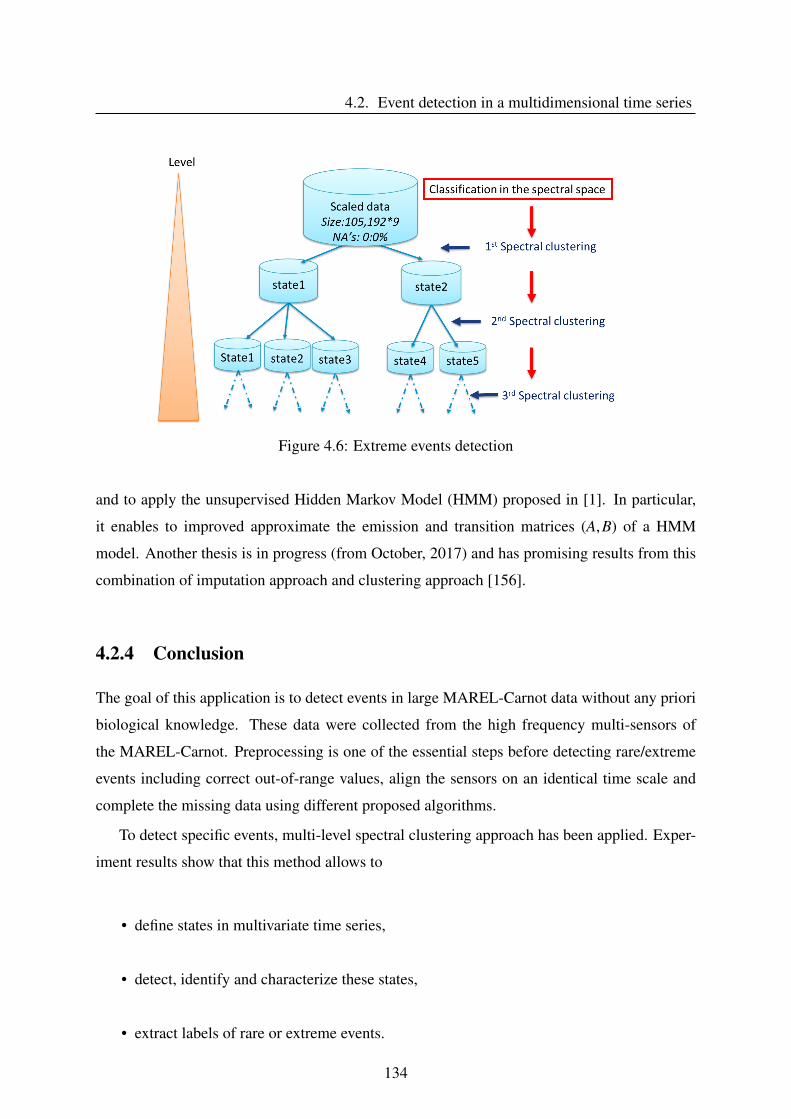
4.2. Event detection in a multidimensional time series
Figure 4.6: Extreme events detection
and to apply the unsupervised Hidden Markov Model (HMM) proposed in [1]. In particular,
it enables to improved approximate the emission and transition matrices (A,B) of a HMM
model. Another thesis is in progress (from October, 2017) and has promising results from this
combination of imputation approach and clustering approach [156].
4.2.4 Conclusion
The goal of this application is to detect events in large MAREL-Carnot data without any priori
biological knowledge. These data were collected from the high frequency multi-sensors of
the MAREL-Carnot. Preprocessing is one of the essential steps before detecting rare/extreme
events including correct out-of-range values, align the sensors on an identical time scale and
complete the missing data using different proposed algorithms.
To detect specific events, multi-level spectral clustering approach has been applied. Exper-
iment results show that this method allows to
• define states in multivariate time series,
• detect, identify and characterize these states,
• extract labels of rare or extreme events.
134
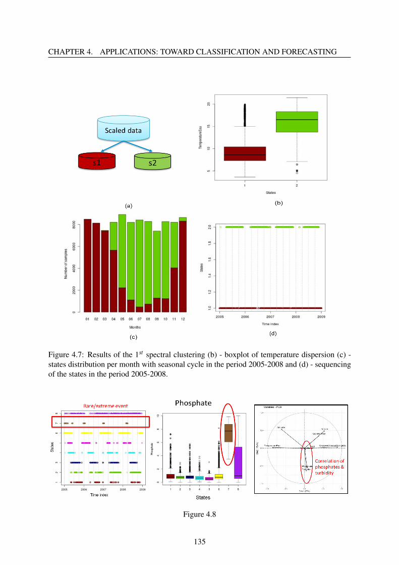
CHAPTER 4. APPLICATIONS: TOWARD CLASSIFICATION AND FORECASTING
Figure 4.7: Results of the 1st spectral clustering (b) - boxplot of temperature dispersion (c) -states distribution per month with seasonal cycle in the period 2005-2008 and (d) - sequencingof the states in the period 2005-2008.
Figure 4.8
135
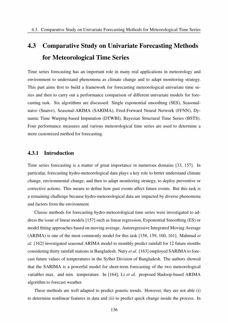
4.3. Comparative Study on Univariate Forecasting Methods for Meteorological Time Series
4.3 Comparative Study on Univariate Forecasting Methods
for Meteorological Time Series
Time series forecasting has an important role in many real applications in meteorology and
environment to understand phenomena as climate change and to adapt monitoring strategy.
This part aims first to build a framework for forecasting meteorological univariate time se-
ries and then to carry out a performance comparison of different univariate models for fore-
casting task. Six algorithms are discussed: Single exponential smoothing (SES), Seasonal-
naive (Snaive), Seasonal-ARIMA (SARIMA), Feed-Forward Neural Network (FFNN), Dy-
namic Time Warping-based Imputation (DTWBI), Bayesian Structural Time Series (BSTS).
Four performance measures and various meteorological time series are used to determine a
more customized method for forecasting.
4.3.1 Introduction
Time series forecasting is a matter of great importance in numerous domains [33, 157]. In
particular, forecasting hydro-meteorological data plays a key role to better understand climate
change, environmental change, and then to adapt monitoring strategy, to deploy preventive or
corrective actions. This means to define how past events affect future events. But this task is
a remaining challenge because hydro-meteorological data are impacted by diverse phenomena
and factors from the environment.
Classic methods for forecasting hydro-meteorological time series were investigated to ad-
dress the issue of linear models [157] such as linear regression, Exponential Smoothing (ES) or
model fitting approaches based on moving average. Autoregressive Integrated Moving Average
(ARIMA) is one of the most commonly model for this task [158, 159, 160, 161]. Mahmud et
al. [162] investigated seasonal ARIMA model to monthly predict rainfall for 12 future months
considering thirty rainfall stations in Bangladesh. Nury et al. [163] employed SARIMA to fore-
cast future values of temperatures in the Sylhet Division of Bangladesh. The authors showed
that the SARIMA is a powerful model for short-term forecasting of the two meteorological
variables max. and min. temperature. In [164], Li et al. proposed Hadoop-based ARIMA
algorithm to forecast weather.
These methods are well adapted to predict generic trends. However, they are not able (i)
to determine nonlinear features in data and (ii) to predict quick change inside the process. In
136
CHAPTER 4. APPLICATIONS: TOWARD CLASSIFICATION AND FORECASTING
the three past decades, numerous approaches have been proposed to improve accuracy and
efficiency of time series forecasting, especially using nonlinear models. Cheng et al. [165]
pointed out that nonlinear models outperform linear ones for time series forecasting in many
applications, such as stock prices [33] and climatology [166].
Artificial Neural Networks (ANN) have become a useful approach to model nonlinear pro-
cesses such as forecasting rainfall [167, 168], or predicting sea level [169]. In [170], Hung et
al. investigated feed-forward neural network model and compared it with a simple persistent
method for hourly rainfall forecasting (from 75 rain gauge stations) in Bangkok, Thailand. The
results showed that FFNN model illustrated better ability to predict rainfall. Chattopadhyay
and Chattopadhya [171] performed a comparison of traditional statistical autoregressive mod-
els and autoregressive NN model for univariate prediction of rainfall time series. The results
of these studies present the improved performance of NN model when comparing it with the
traditional statistical approaches.
Dynamic Time Warping (DTW) [7] is an effective method for measuring similarity between
two linear/nonlinear time series. This method is successfully applied in pattern recognition
[9, 10], in imputation [90]. For the forecasting task, there are few studies using DTW to predict
future values. In [172] Tsinaslanidis and Kugiumtzis used perceptually important points and
DTW for stock market forecasting.
Compared to other methods, only few research has been devoted to predict time series using
a Bayesian network-based method, although Aguilera et al. showed the capability of Bayesian
networks in environmental modeling in [173].
Thus this work does not propose a novel forecasting method. However we emphasize
on comparing the performances of different univariate approaches by building a framework
for forecasting hydro-meteorological univariate time series. Five time series data are applied
to the six models we choose for anticipating future values including SES, Snaive, SARIMA,
FFNN, DTWBI, and BSTS. This allows to suggest the most suitable method, among the above-
mentioned methods, for predicting hydro-meteorological univariate time series ensuring that
results are reliable and of high quality.
In addition, for univariate forecasting methods, we must only rely on the available values
of this unique variable to estimate future values, without other outside explanatory variables
[174]. And, Smith and Agrawal [175] pointed out that "when attempting to forecast univariate
time series data, it is generally accepted that parsimonious model techniques are followed.
In the next section, we focus on univariate forecasting methods. Then, Section 4.3.3 intro-
137
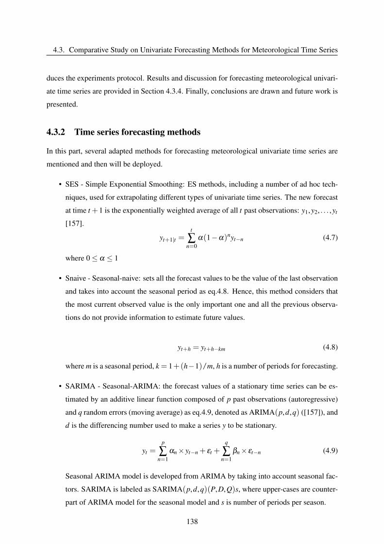
4.3. Comparative Study on Univariate Forecasting Methods for Meteorological Time Series
duces the experiments protocol. Results and discussion for forecasting meteorological univari-
ate time series are provided in Section 4.3.4. Finally, conclusions are drawn and future work is
presented.
4.3.2 Time series forecasting methods
In this part, several adapted methods for forecasting meteorological univariate time series are
mentioned and then will be deployed.
• SES - Simple Exponential Smoothing: ES methods, including a number of ad hoc tech-
niques, used for extrapolating different types of univariate time series. The new forecast
at time t +1 is the exponentially weighted average of all t past observations: y1,y2, . . . ,yt
[157].
yt+1|t =t
∑n=0
α(1−α)nyt−n (4.7)
where 0≤ α ≤ 1
• Snaive - Seasonal-naive: sets all the forecast values to be the value of the last observation
and takes into account the seasonal period as eq.4.8. Hence, this method considers that
the most current observed value is the only important one and all the previous observa-
tions do not provide information to estimate future values.
yt+h = yt+h−km (4.8)
where m is a seasonal period, k = 1+(h−1)/m, h is a number of periods for forecasting.
• SARIMA - Seasonal-ARIMA: the forecast values of a stationary time series can be es-
timated by an additive linear function composed of p past observations (autoregressive)
and q random errors (moving average) as eq.4.9, denoted as ARIMA(p,d,q) ([157]), and
d is the differencing number used to make a series y to be stationary.
yt =p
∑n=1
αn× yt−n + εt +q
∑n=1
βn× εt−n (4.9)
Seasonal ARIMA model is developed from ARIMA by taking into account seasonal fac-
tors. SARIMA is labeled as SARIMA(p,d,q)(P,D,Q)s, where upper-cases are counter-
part of ARIMA model for the seasonal model and s is number of periods per season.
138
CHAPTER 4. APPLICATIONS: TOWARD CLASSIFICATION AND FORECASTING
• BSTS - Bayesian Structural Time Series: This model applies Markov Chain Monte Carlo
(MCMC) to sample the posterior distribution of a Bayesian structural time series model.
The model involves 3 major steps:
Kalman filter: This step consists in decomposing a time series. Various state variables
such as trend, seasonality, regression can be added in this step.
Spike-and-slab: This step selects the most important regression predictors.
Bayesian model averaging: This step combines the results and calculates prediction val-
ues.
• DTWBI: In a previous study [90], we proposed DTWBI approach for completing missing
values. Here, we consider forecasting values as missing data, and then we apply DTWBI
method to compute these future values. Forecasting process is based on past values.
This is fully compatible with DTWBI approach that fills missing values according to the
recorded data.
Figure 4.9: Illustration of the DTWBI for the forecasting task: 1-Query building, 2-Slidingwindow comparison, 3-Window selection, 4-Forecasting values
The approach consists in finding the most similar sub-sequence Qs to a query Q (the sub-
sequence before the predicted position) by sliding windows based on the combination of
shape-feature extraction algorithm [52] and DTW method. This allows some distortions
139
4.3. Comparative Study on Univariate Forecasting Methods for Meteorological Time Series
both in the temporal and value axis. Once the most similar window is identified, the
following sub-sequence Q f s of the Qs is considered as the forecast values. The dynamics
and the shape of data before the forecast values are key-point of this technique (see [90]).
• FFNN - Feed-forward neural network: Artificial Neural Network is proposed from in-
spiring the interconnection neurons of the human. FFNN maps the set of inputs to the
set of outputs (both data inputs and outputs are digital). FFNN allows to automatically
extract global features before the last decision step (output layer) considering only one
hidden layer. A FFNN with no hidden layers is also called linear perceptron: its inputs
are directly mapped to the outputs unit via the weighted connections.
4.3.3 Experiment protocol
We have performed a set of experiments on five meteorological time series using six different
univariate models to evaluate their forecasting performance.
4.3.3.1 Experiment set up
R language is used to conduct all experiments. We utilize the latest forecast R-packages [176]
(for FFNN, Ses and Snaive), astsa [177] for SARIMA, bsts [178] (for BSTS). For DTWBI, we
develop ourselves (upon request). For SARIMA, auto.arima() [176] is employed to optimize
the parameters p,d,q,P,D,Q. For FFNN, we use the default parameters: input nodes are the
number of seasonal lags applied to seasonally adjusted data, and number of nodes in the single
hidden layer is half the number of input nodes. And for BSTS, we choose niter = 50 with
specified seasonality component for each forecasting rate.
4.3.3.2 Data presentation
In this section, we describe the data used for the study. Five hydro-meteorological time series
are used for evaluating the performance of forecasting methods (table 4.8). These five datasets
were collected at three meteorological stations in Vietnam. They have different sampling fre-
quency and time measurement duration (short or long period). In order to obtain useful infor-
mation from the datasets and to make the datasets easily exploitable, we analyzed these series.
Table 4.8 summarizes their characteristics. All the five datasets have a seasonality component
(i.e. an annual cycle), without any linear trend.
140
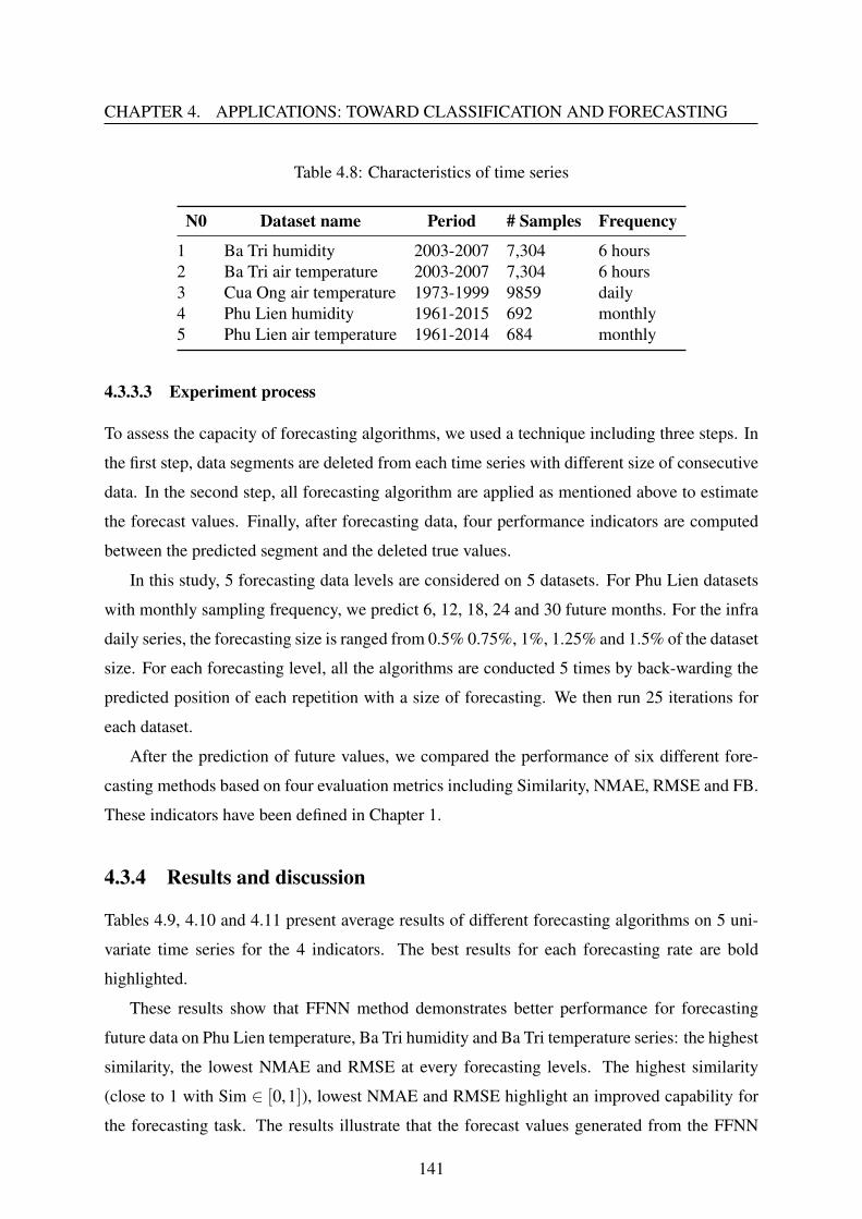
CHAPTER 4. APPLICATIONS: TOWARD CLASSIFICATION AND FORECASTING
Table 4.8: Characteristics of time series
N0 Dataset name Period # Samples Frequency
1 Ba Tri humidity 2003-2007 7,304 6 hours2 Ba Tri air temperature 2003-2007 7,304 6 hours3 Cua Ong air temperature 1973-1999 9859 daily4 Phu Lien humidity 1961-2015 692 monthly5 Phu Lien air temperature 1961-2014 684 monthly
4.3.3.3 Experiment process
To assess the capacity of forecasting algorithms, we used a technique including three steps. In
the first step, data segments are deleted from each time series with different size of consecutive
data. In the second step, all forecasting algorithm are applied as mentioned above to estimate
the forecast values. Finally, after forecasting data, four performance indicators are computed
between the predicted segment and the deleted true values.
In this study, 5 forecasting data levels are considered on 5 datasets. For Phu Lien datasets
with monthly sampling frequency, we predict 6, 12, 18, 24 and 30 future months. For the infra
daily series, the forecasting size is ranged from 0.5% 0.75%, 1%, 1.25% and 1.5% of the dataset
size. For each forecasting level, all the algorithms are conducted 5 times by back-warding the
predicted position of each repetition with a size of forecasting. We then run 25 iterations for
each dataset.
After the prediction of future values, we compared the performance of six different fore-
casting methods based on four evaluation metrics including Similarity, NMAE, RMSE and FB.
These indicators have been defined in Chapter 1.
4.3.4 Results and discussion
Tables 4.9, 4.10 and 4.11 present average results of different forecasting algorithms on 5 uni-
variate time series for the 4 indicators. The best results for each forecasting rate are bold
highlighted.
These results show that FFNN method demonstrates better performance for forecasting
future data on Phu Lien temperature, Ba Tri humidity and Ba Tri temperature series: the highest
similarity, the lowest NMAE and RMSE at every forecasting levels. The highest similarity
(close to 1 with Sim ∈ [0,1]), lowest NMAE and RMSE highlight an improved capability for
the forecasting task. The results illustrate that the forecast values generated from the FFNN
141
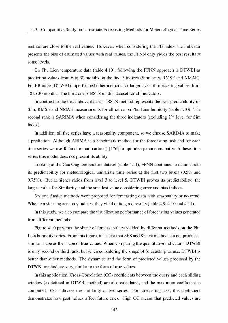
4.3. Comparative Study on Univariate Forecasting Methods for Meteorological Time Series
method are close to the real values. However, when considering the FB index, the indicator
presents the bias of estimated values with real values, the FFNN only yields the best results at
some levels.
On Phu Lien temperature data (table 4.10), following the FFNN approach is DTWBI as
predicting values from 6 to 30 months on the first 3 indices (Similarity, RMSE and NMAE).
For FB index, DTWBI outperformed other methods for larger sizes of forecasting values, from
18 to 30 months. The third one is BSTS on this dataset for all indicators.
In contrast to the three above datasets, BSTS method represents the best predictability on
Sim, RMSE and NMAE measurements for all ratios on Phu Lien humidity (table 4.10). The
second rank is SARIMA when considering the three indicators (excluding 2nd level for Sim
index).
In addition, all five series have a seasonality component, so we choose SARIMA to make
a prediction. Although ARIMA is a benchmark method for the forecasting task and for each
time series we use R function auto.arima() [176] to optimize parameters but with these time
series this model does not present its ability.
Looking at the Cua Ong temperature dataset (table 4.11), FFNN continues to demonstrate
its predictability for meteorological univariate time series at the first two levels (0.5% and
0.75%). But at higher ratios from level 3 to level 5, DTWBI proves its predictability: the
largest value for Similarity, and the smallest value considering error and bias indices.
Ses and Snaive methods were proposed for forecasting data with seasonality or no trend.
When considering accuracy indices, they yield quite good results (table 4.9, 4.10 and 4.11).
In this study, we also compare the visualization performance of forecasting values generated
from different methods.
Figure 4.10 presents the shape of forecast values yielded by different methods on the Phu
Lien humidity series. From this figure, it is clear that SES and Snaive methods do not produce a
similar shape as the shape of true values. When comparing the quantitative indicators, DTWBI
is only second or third rank, but when considering the shape of forecasting values, DTWBI is
better than other methods. The dynamics and the form of predicted values produced by the
DTWBI method are very similar to the form of true values.
In this application, Cross-Correlation (CC) coefficients between the query and each sliding
window (as defined in DTWBI method) are also calculated, and the maximum coefficient is
computed. CC indicates the similarity of two series. For forecasting task, this coefficient
demonstrates how past values affect future ones. High CC means that predicted values are
142
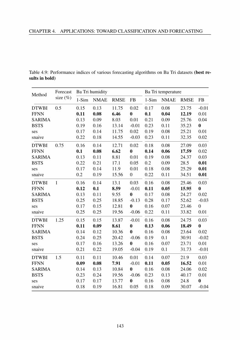
CHAPTER 4. APPLICATIONS: TOWARD CLASSIFICATION AND FORECASTING
Table 4.9: Performance indices of various forecasting algorithms on Ba Tri datasets (best re-sults in bold)
MethodForecastsize (%)
Ba Tri humidity Ba Tri temperature
1-Sim NMAE RMSE FB 1-Sim NMAE RMSE FB
DTWBI 0.5 0.15 0.13 11.75 0.02 0.17 0.08 23.75 -0.01FFNN 0.11 0.08 6.46 0 0.1 0.04 12.19 0.01SARIMA 0.13 0.09 8.03 0.01 0.21 0.09 25.76 0.04BSTS 0.19 0.16 13.14 -0.01 0.23 0.11 35.23 0ses 0.17 0.14 11.75 0.02 0.19 0.08 25.21 0.01snaive 0.22 0.18 14.55 -0.03 0.23 0.11 32.35 0.02
DTWBI 0.75 0.16 0.14 12.71 0.02 0.18 0.08 27.09 0.03FFNN 0.1 0.08 6.62 0 0.14 0.06 17.59 0.02SARIMA 0.13 0.11 8.81 0.01 0.19 0.08 24.37 0.03BSTS 0.22 0.21 17.1 0.05 0.2 0.09 28.5 0.01ses 0.17 0.14 11.9 0.01 0.18 0.08 25.29 0.01snaive 0.2 0.19 15.56 0 0.22 0.11 34.51 0.01
DTWBI 1 0.16 0.14 13.1 0.03 0.16 0.08 25.46 0.03FFNN 0.12 0.1 8.59 -0.01 0.11 0.05 15.95 0SARIMA 0.13 0.11 9.55 0 0.17 0.08 24.27 0.02BSTS 0.25 0.25 18.85 -0.13 0.28 0.17 52.62 -0.03ses 0.17 0.15 12.81 0 0.16 0.07 23.46 0snaive 0.25 0.25 19.56 -0.06 0.22 0.11 33.82 0.01
DTWBI 1.25 0.15 0.15 13.87 -0.01 0.16 0.08 24.75 0.03FFNN 0.11 0.09 8.61 0 0.13 0.06 18.49 0SARIMA 0.14 0.12 10.36 0 0.16 0.08 23.64 0.02BSTS 0.24 0.25 20.42 -0.06 0.19 0.1 30.91 -0.02ses 0.17 0.16 13.26 0 0.16 0.07 23.71 0.01snaive 0.21 0.22 19.05 -0.04 0.19 0.1 31.73 -0.01
DTWBI 1.5 0.11 0.11 10.46 0.01 0.14 0.07 21.9 0.03FFNN 0.09 0.08 7.91 -0.01 0.11 0.05 16.52 0.01SARIMA 0.14 0.13 10.84 0 0.16 0.08 24.06 0.02BSTS 0.23 0.24 19.56 -0.06 0.23 0.13 40.17 0.01ses 0.17 0.17 13.77 0 0.16 0.08 24.8 0snaive 0.18 0.19 16.81 0.05 0.18 0.09 30.07 -0.04
143
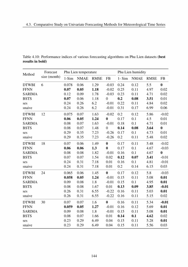
4.3. Comparative Study on Univariate Forecasting Methods for Meteorological Time Series
Table 4.10: Performance indices of various forecasting algorithms on Phu Lien datasets (bestresults in bold)
MethodForecast
size (month)Phu Lien temperature Phu Lien humidity
1-Sim NMAE RMSE FB 1- Sim NMAE RMSE FB
DTWBI 6 0.078 0.06 1.29 -0.03 0.24 0.12 5.5 0FFNN 0.07 0.05 1.18 -0.02 0.25 0.11 4.97 0.02SARIMA 0.12 0.09 1.78 -0.03 0.23 0.11 4.71 0.02BSTS 0.07 0.06 1.18 0 0.2 0.08 3.51 0.01ses 0.24 0.26 6.2 -0.01 0.22 0.11 4.84 0.02snaive 0.24 0.26 6.2 -0.01 0.31 0.17 6.99 0.06
DTWBI 12 0.075 0.07 1.63 -0.02 0.2 0.12 5.86 -0.02FFNN 0.06 0.05 1.24 0 0.17 0.1 4.5 0.01SARIMA 0.08 0.07 1.63 -0.01 0.18 0.1 4.71 0.01BSTS 0.08 0.07 1.48 0 0.14 0.08 3.64 0ses 0.29 0.35 7.23 -0.26 0.17 0.1 4.73 0.01snaive 0.29 0.35 7.23 -0.26 0.2 0.11 5.48 0.02
DTWBI 18 0.07 0.06 1.49 0 0.17 0.11 5.48 -0.02FFNN 0.06 0.06 1.3 0 0.17 0.1 4.67 -0.03SARIMA 0.08 0.08 1.82 -0.01 0.16 0.1 4.67 0BSTS 0.07 0.07 1.54 0.02 0.12 0.07 3.41 -0.01ses 0.24 0.31 7.18 0.01 0.16 0.1 4.81 -0.01snaive 0.24 0.31 7.18 0.01 0.2 0.14 6.15 0.03
DTWBI 24 0.065 0.06 1.45 0 0.17 0.12 5.8 -0.03FFNN 0.058 0.05 1.24 -0.01 0.15 0.11 5.08 0.01SARIMA 0.09 0.08 1.8 -0.01 0.15 0.1 4.95 0.01BSTS 0.08 0.08 1.67 0.01 0.13 0.09 3.85 -0.01ses 0.26 0.31 6.55 -0.22 0.16 0.11 5.03 0.01snaive 0.26 0.31 6.55 -0.22 0.16 0.11 5.15 0.02
DTWBI 30 0.07 0.07 1.6 0 0.16 0.11 5.34 -0.01FFNN 0.059 0.05 1.27 -0.01 0.16 0.12 5.69 0.01SARIMA 0.09 0.08 1.8 -0.01 0.15 0.11 5.08 0.01BSTS 0.08 0.07 1.66 0.01 0.14 0.1 4.62 0.02ses 0.23 0.29 6.49 0.04 0.15 0.11 5.28 0.01snaive 0.23 0.29 6.49 0.04 0.15 0.11 5.56 0.03
144
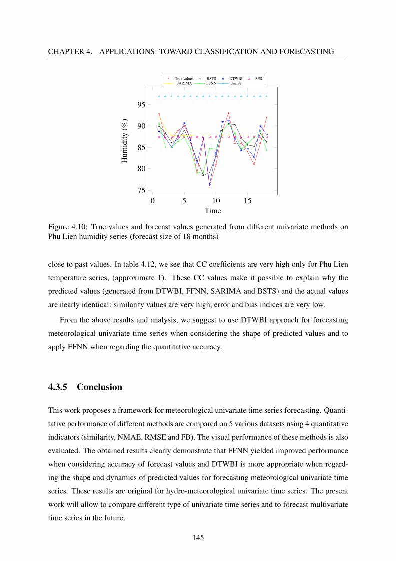
CHAPTER 4. APPLICATIONS: TOWARD CLASSIFICATION AND FORECASTING
0 5 10 1575
80
85
90
95
Time
Hum
idity
(%)
True values BSTS DTWBI SESSARIMA FFNN Snaive
Figure 4.10: True values and forecast values generated from different univariate methods onPhu Lien humidity series (forecast size of 18 months)
close to past values. In table 4.12, we see that CC coefficients are very high only for Phu Lien
temperature series, (approximate 1). These CC values make it possible to explain why the
predicted values (generated from DTWBI, FFNN, SARIMA and BSTS) and the actual values
are nearly identical: similarity values are very high, error and bias indices are very low.
From the above results and analysis, we suggest to use DTWBI approach for forecasting
meteorological univariate time series when considering the shape of predicted values and to
apply FFNN when regarding the quantitative accuracy.
4.3.5 Conclusion
This work proposes a framework for meteorological univariate time series forecasting. Quanti-
tative performance of different methods are compared on 5 various datasets using 4 quantitative
indicators (similarity, NMAE, RMSE and FB). The visual performance of these methods is also
evaluated. The obtained results clearly demonstrate that FFNN yielded improved performance
when considering accuracy of forecast values and DTWBI is more appropriate when regard-
ing the shape and dynamics of predicted values for forecasting meteorological univariate time
series. These results are original for hydro-meteorological univariate time series. The present
work will allow to compare different type of univariate time series and to forecast multivariate
time series in the future.
145
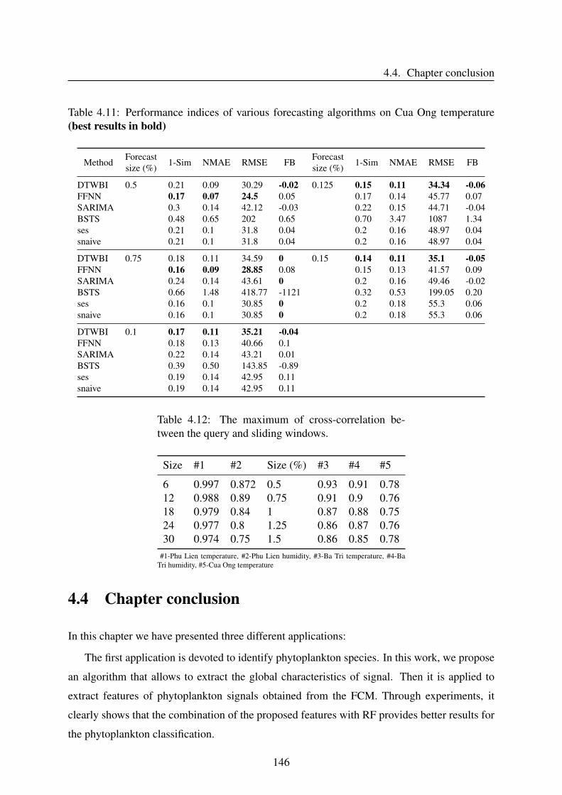
4.4. Chapter conclusion
Table 4.11: Performance indices of various forecasting algorithms on Cua Ong temperature(best results in bold)
MethodForecastsize (%) 1-Sim NMAE RMSE FB
Forecastsize (%) 1-Sim NMAE RMSE FB
DTWBI 0.5 0.21 0.09 30.29 -0.02 0.125 0.15 0.11 34.34 -0.06FFNN 0.17 0.07 24.5 0.05 0.17 0.14 45.77 0.07SARIMA 0.3 0.14 42.12 -0.03 0.22 0.15 44.71 -0.04BSTS 0.48 0.65 202 0.65 0.70 3.47 1087 1.34ses 0.21 0.1 31.8 0.04 0.2 0.16 48.97 0.04snaive 0.21 0.1 31.8 0.04 0.2 0.16 48.97 0.04
DTWBI 0.75 0.18 0.11 34.59 0 0.15 0.14 0.11 35.1 -0.05FFNN 0.16 0.09 28.85 0.08 0.15 0.13 41.57 0.09SARIMA 0.24 0.14 43.61 0 0.2 0.16 49.46 -0.02BSTS 0.66 1.48 418.77 -1121 0.32 0.53 199.05 0.20ses 0.16 0.1 30.85 0 0.2 0.18 55.3 0.06snaive 0.16 0.1 30.85 0 0.2 0.18 55.3 0.06
DTWBI 0.1 0.17 0.11 35.21 -0.04FFNN 0.18 0.13 40.66 0.1SARIMA 0.22 0.14 43.21 0.01BSTS 0.39 0.50 143.85 -0.89ses 0.19 0.14 42.95 0.11snaive 0.19 0.14 42.95 0.11
Table 4.12: The maximum of cross-correlation be-tween the query and sliding windows.
Size #1 #2 Size (%) #3 #4 #5
6 0.997 0.872 0.5 0.93 0.91 0.7812 0.988 0.89 0.75 0.91 0.9 0.7618 0.979 0.84 1 0.87 0.88 0.7524 0.977 0.8 1.25 0.86 0.87 0.7630 0.974 0.75 1.5 0.86 0.85 0.78
#1-Phu Lien temperature, #2-Phu Lien humidity, #3-Ba Tri temperature, #4-BaTri humidity, #5-Cua Ong temperature
4.4 Chapter conclusion
In this chapter we have presented three different applications:
The first application is devoted to identify phytoplankton species. In this work, we propose
an algorithm that allows to extract the global characteristics of signal. Then it is applied to
extract features of phytoplankton signals obtained from the FCM. Through experiments, it
clearly shows that the combination of the proposed features with RF provides better results for
the phytoplankton classification.
146
CHAPTER 4. APPLICATIONS: TOWARD CLASSIFICATION AND FORECASTING
In the second application, we have applied the DTWBI algorithm to fill in large gaps, and
two other algorithms to complete small gaps in the MAREL-Carnot dataset. We then have
employed a multi-level spectral clustering approach to detect events in the data without any
biological prior knowledge. The results show that this protocol allows to (i) determine states
in multivariate time series; (ii) detect, identify and characterize states, for example, detecting
inaccurate data in the salinity range; and (iii) extract labels of rare/extreme events.
The third application focuses on comparing of different univariate forecasting methods for
meteorological time series. In this work, we also apply DTWBI to predict future values. Ex-
periments show that DTWBI gives improved results when considering the shape of forecast
values.
List of Publications and valuations related to this chapter
1. Thi-Thu-Hong Phan, Emilie Poisson Caillault, André Bigand, "Comparative Study on
Univariate Forecasting Methods for Meteorological Time Series", 26th European Signal
Processing Conference. Eusipco 2018. September 3-7, 2018, Rome, Italy.
2. Thi-Thu-Hong Phan, Emilie Poisson Caillault, André Bigand, "Comparative Study on
Supervised Learning Methods for Identifying Phytoplankton Species", 2016 IEEE Sixth
International Conference on Communications and Electronics (IEEE ICCE 2016). Full
Accepted paper. July 27 - 29, 2016. Ha Long, Vietnam. DOI: 10.1109/CCE.2016.7562650
3. Lefebvre A., Grassi K., Phan T.T.H., Devreker D., Bigand A., Poisson-Caillault E., 2018,
"Automated tools for analyzing outputs of automated sensors: High frequency Data",
Third JERICO-NEXT Workshop on Phytoplankton Automated Observation. March 19-
21, 2018 - M.I.O., Marseille, France.
4. Grassi K., Phan T.T.H., Poisson-Caillault E., Bigand A., Devreker D., Lefebvre A., "Re-
sults from measurements in the eastern English Channel : MAREL Carnot station", Third
JERICO-NEXT Workshop on Phytoplankton Automated Observation. March 19-21,
2018 - M.I.O., Marseille, France.
147

4.4. Chapter conclusion
148
Conclusions and future work
Conclusions
Missing data are the first weakness of most statistical models and data analysis methods. De-
spite their suitability of performances, missing data make them unable to operate. Completing
missing data is a necessary precondition for a majority of approaches. Therefore, in this work
we present our research on the missing data problem. The main contribution is the investi-
gation and development of different techniques to impute large consecutive missing values in
time series data. We focus on two types of data: univariate and uncorrelated multivariate time
series. In the special case of those two types of time series, the imputation task is a remaining
challenge because we cannot take advantage of inter-variable correlations to estimate missing
values. Hence, we must exploit observed data in the incomplete time series itself to compute
missing data.
The first main objective of this study is the proposition of an effective method to fill large
missing values in univariate time series. In this context, we take into account time series char-
acteristics to develop an appropriate and efficient strategy. We have opted for the elastic match-
ing approach combined with a shape-feature extraction algorithm to propose DTWBI method.
Experiments carried out on well-known and real-world datasets show that the completion of
missing data by finding the most similar sequences using the elastic matching is a robust solu-
tion. Looking for similar sequences by elastic matching enables to complete missing values in
database while conserving as much as possible the dynamics and the shape of signals. Using
the shape-feature extraction algorithm greatly decreases the computing time. In addition, we
study different variants of the DTW approach (including DDTW, AFBDTW and DTW-D) and
in particular we focus on the comparison of these variants for the univariate imputation task.
149
4.4. Chapter conclusion
The objective of this comparison is to suggest the most adaptable version to fill incompleteness
in univariate time series according to the desired goal. Experimental results point out that when
considering the accuracy of imputation values, DTW is more convenient and when regarding
the shape of imputation values for the large gaps and big datasets, AFBDTW is more suitable.
The second major goal of this study is to deal with missing values in low/un-correlated mul-
tivariate time series. In the literature, most proposed approaches address the missing problem in
correlated multivariate data by taking advantage of the relations between variables. Fewer stud-
ies pay attention to solve the incompleteness issue in low/un-correlated multivariate time series.
Thus, we have investigated two algorithms to complete large missing values in low/uncorrelated
multivariate data by exploiting the propriety of this type of data.
The first algorithm is an extension of DTWBI, namely DTWUMI (DTW-Uncorrelated Mul-
tivariate Imputation). As in DTWBI, we based our approach on the combination of DTW
method and shape-feature extraction algorithm. DTWUMI’s originality consists in a conjoint
multivariate matching. So, we take care of the time index of all the variables. This is shown
in the query creation (a matrix of all the variables before or after a gap) and finding similar
windows steps. However, only a vector following (or preceding) of the most similar window in
the signal containing the considered gap is used to complete the gap.
The second algorithm, namely FSMUMI, takes into account a factor of uncertainty. In
this way, we develop a novel similarity measure based on fuzzy grades of basic similarity
measures and fuzzy logic rules. In other words, the characteristic of low/un-correlation data
is also exploited. Each signal is individually processed. Then, for each gap in this individual
signal, we consider the data before this gap and after the gap as two separated univariate time
series. The novel fuzzy-weighted similarity measure is applied to find similar windows in each
univariate time series. Once imputation values from two separated time series are available, the
gap is completed by averaging the both vectors of imputation values.
Experimental results on simulated and real datasets show that both proposed algorithms
provide improved performance for the imputation task, not only in accuracy indices but also in
the shape of imputation values. Moreover, they are capable of solving the problem of wholly
missing variables (missing rows problem).
In this study, in addition to the investigation of various imputation techniques, we have also
proposed an algorithm to extract global characteristics of signal (called the shape-feature ex-
traction algorithm). This method is then applied to compute features of phytoplankton signals.
Through experiments, it clearly indicates that the combination of the proposed features with
150
CHAPTER 4. APPLICATIONS: TOWARD CLASSIFICATION AND FORECASTING
Random Forest provides better results for the phytoplankton classification. The shape-feature
extraction algorithm is also combined with DTW approach in the two previous proposed algo-
rithms (DTWBI and DTWUMI), with the aim of reducing the calculation time.
Besides, in this thesis DTWBI is applied in two specific applications. Experimental results
are very promising:
In the first application, DTWBI is employed to complete large gaps in the MAREL Carnot
dataset, then a multi-level spectral clustering approach is performed to detect rare/extreme
events in the data without any prior biological knowledge. The results show that this proto-
col is able to detect/identify and characterize states and to extract labels of rare/extreme events.
In the second application, DTWBI is devoted to forecast meteorological univariate time
series (section 4.3). We are based this work on the idea of imputation to predict future values
in meteorological univariate time series. Experiments are conducted on five different univariate
meteorological time series collected in Vietnam. The obtained results illustrate that DTWBI
gives improved performance when considering the shape of forecast values.
Perspectives for future work
Based on the results presented in this thesis, we will now detail several perspectives for future
research directions to improve the overall system.
Improvement of the performance of imputation algorithms
• In this thesis we propose DTWBI algorithm, which enables to impute large consecutive
missing values in univariate time series, based on the combination of the shape-feature
extraction and elastic matching approaches. This method is evaluated and compared with
state-of-the-art approaches which do not allow to complete large periods of lacking data
(detailed in Chapter 2). The obtained results are encouraging but in the DTWBI algorithm
we only consider one query either before or after the considered gap. Therefore, an
investigation of this algorithm should be expanded by taking into account two queries,
one query before and one query after the gap. Moreover, data before and data after the
gap will be considered as two referenced time series. This would, on the one hand, enrich
the learning base and, consequently, improve the prediction ability of the method. On the
other hand, this permits to envisage dynamics (important key) of data before and after
151
4.4. Chapter conclusion
the gap to estimate imputation values.
• In the third proposal of this report, we develope a new fuzzy weighted-based similarity
measure to fill large consecutive incompleteness in low/un-correlated multivariate time
series (Chapter 3). Although this approach meets requirements and illustrates appealing
results but there is still place for further development. The hybrid similarity measure is
built based on fuzzy grades of basic similarity measures and on fuzzy-based rules (built
from ordinary fuzzy set). Type-2 fuzzy set (T2FS) can handle more uncertainty because
their membership functions are fuzzy themselves. So that T2FS should be investigated
to solve missing data problems in both types of time series: univariate and multivariate
time series using a new similarity measure for example.
• In the DTWUMI proposal, we initially use the trapezoid function to estimate initial val-
ues for missing data. With the promising results of the FSMUMI algorithm, we intend
to use this algorithm instead of the trapezoid function in the DTWUMI algorithm to
complete missing data.
• In the present work, we propose two algorithms to complete large missing values in
low/un-correlated multivariate time series (Chapter 3). Experiment results show that
the proposed algorithms provide improved performance for the imputation task. But in
these studies, we only focus on dealing with large gaps in multivariate time series having
low/un-correlation. Another solution would be studied to complete missing values in any
type of multivariate time series by combining the proposed methods with other powerful
approaches, for example Deep learning or random forest (RF).
Applications
• A further investigation on how to forecast multivariate time series can be conducted. As
presented in Chapter 4, we have applied DTWBI for forecasting meteorological univari-
ate time series. Results obtained are also promising and reliable. However, in the litera-
ture few studies have focused on multivariate time series forecasting. It would be interest-
ing to investigate multivariate forecasting time series with a performance improvement.
• In this study, the detection of extreme/rare events in MAREL Carnot dataset using an
unsupervised method (multi-level spectral clustering) has been discussed in Chapter 4.
152
CHAPTER 4. APPLICATIONS: TOWARD CLASSIFICATION AND FORECASTING
Moreover, for imputation applications, we have applied similarity measures for retrieving
similar subsequences (Chapter 2 and 3). For anomaly detection application, the similar-
ity measure is also an important key to determine "how closely matched are two given
observations" ([179]). Motivated from this, future research and further developments
of anomaly detection in univariate/multivariate by using similarity measures could be
considered.
• In Chapter 4, the shape-feature extraction algorithm is proposed and then applied to clas-
sify phytoplankton species. In section 4.1, a better ability for the classification task when
combining RF and the proposed features is pointed out. Nevertheless, an improvement
of this identification framework could be implemented as follows: firstly, we could com-
bine different types of features, then apply feature-selection methods to select meaningful
features which will be used to identify phytoplankton species. This would to extend our
work in other learning contexts.
153

4.4. Chapter conclusion
154

Appendices
155

Appendix AList of publications and valuations related to
the thesis
1. International journals with peer review
• Thi-Thu-Hong Phan, Emilie Poisson Caillault, Alain Lefebvre, André Bigand, "Dy-
namic Time Warping-based imputation for univariate time series data", Pattern
Recognition Letters. Available online 16 August 2017. In Press.
DOI: 10.1016/j.patrec.2017.08.019
• Thi-Thu-Hong Phan, André Bigand, Emilie Poisson Caillault, "A New Fuzzy Logic-
based Similarity Measure applied to Large Gap Imputation for Uncorrelated Mul-
tivariate Time Series", Applied Computational Intelligence and Soft Computing.
Available online August 2018.
DOI: 10.1155/2018/9095683
2. International conferences with peer review
• Thi-Thu-Hong Phan, Emilie Poisson Caillault, André Bigand, "Comparative Study
on Univariate Forecasting Methods for Meteorological Time Series", 26th European
Signal Processing Conference. Eusipco 2018. September 3-7, 2018, Rome, Italy.
• Thi-Thu-Hong Phan, Emilie Poisson Caillault, Alain Lefebvre, André Bigand, "DTW-
Approach For Uncorrelated Multivariate Time Series Imputation", IEEE Interna-
tional Workshop on Machine Learning for Signal Processing. MLSP 2017. Septem-
ber 25-28, 2017 Roppongi, Tokyo, Japan. DOI: 10.1109/MLSP.2017.8168165
157
• Thi-Thu-Hong Phan, Emilie Poisson Caillault, Alain Lefebvre, André Bigand, "Which
DTW Method Applied to Marine Univariate Time Series Imputation", OCEANS
2017 MTS/IEEE, Aberdeen, Scotland, 06/2017. DOI: 10.1109/OCEANSE.2017.8084598
• Thi-Thu-Hong Phan, Emilie Poisson Caillault, André Bigand, "Comparative Study
on Supervised Learning Methods for Identifying Phytoplankton Species", 2016
IEEE Sixth International Conference on Communications and Electronics (IEEE
ICCE 2016). Full Accepted paper. July 27 - 29, 2016. Ha Long, Vietnam. DOI:
10.1109/CCE.2016.7562650
3. Communication/National conferences
• Emilie Poisson Caillault, Kelly Grassi, Thi Thu Hong Phan, Camille Dezecache,
Jean Prygiel, Alain Lefebvre, "DTWBI & uHMM R-packages for multivariate time
series preprocessing and interpretation", 26th Earth Science Meeting, 22-26 Octo-
ber 2018, Lille, France.
• Emilie Poisson Caillault, Camille Dezecache, Thi Thu Hong Phan, Kelly Grassi,
Jean Prygiel, and Alain Lefebvre, "Data completion, characterization of environ-
mental states and dynamics using multiparameter time series: DTWBI, DTWUMI
and uHMM R-packages", 2nd General Assembly of JERICO-NEXT, Galway, Ire-
land, 24-27 September, 2018.
• Lefebvre A., Grassi K., Phan T.T.H., Devreker D., Bigand A., Poisson-Caillault
E., 2018, "Automated tools for analyzing outputs of automated sensors: High fre-
quency Data", Third JERICO-NEXT Workshop on Phytoplankton Automated Ob-
servation. March 19-21, 2018 - M.I.O., Marseille, France.
• Grassi K., Phan T.T.H., Poisson-Caillault E., Bigand A., Devreker D., Lefebvre A.,
"Results from measurements in the eastern English Channel : MAREL Carnot sta-
tion", Third JERICO-NEXT Workshop on Phytoplankton Automated Observation.
March 19-21, 2018 - M.I.O., Marseille, France.
• Caillault-Poisson E., Lefebvre A., Hébert P.A., Phan, T.T.H., Ternynck P., Marson
Q., Rizik A., Wacquet G., Artigas F., Bigand A, "Méthodologie(s) du traitement
du signal à la classification/modélisation pour la compréhension de la dynamique
des efflorescences phytoplanctoniques", Journée du CPER MARCO, 26 juin 2017,
Boulogne sur Mer, France.
158

APPENDIX A. LIST OF PUBLICATIONS AND VALUATIONS RELATED TO THETHESIS
• Caillault-Poisson E., Phan, T.T.H., Rizik A., Ternynck P., Bigand A, Lefebvre A,
"New developments to fill the gap in high frequency data series and to integrate
knowledge in Markov modeling of phytoplankton dynamics", EEC’2017: The East-
ern English Channel Conference, Wimereux, 06/06/2017, France.
4. Package
• DWTBI R-package https://cran.r-project.org/web/packages/DTWBI/index.html
• DTWUMI R-package https://cran.r-project.org/web/packages/DTWUMI/index.html
5. Doctoriales
• Thi-Thu-Hong Phan, Emilie Poisson Caillault, Alain Lefebvre, André Bigand. DTW-
Approach For Uncorrelated Multivariate Time Series Imputation, 5th édition de la
Journée Doctorale du Campus de la Mer, 19 October, 2017 Boulogne sur Mer,
France.
• Thi-Thu-Hong Phan, Emilie Poisson Caillault, Alain Lefebvre, André Bigand. Com-
parative Study on Supervised Learning Methods for Identifying Phytoplankton Species,
4th édition de la Journée Doctorale du Campus de la Mer, 20 October, 2016 Boulogne
sur Mer, France.
6. Seminars
• Thi-Thu-Hong Phan, Emilie Poisson Caillault, Alain Lefebvre, André Bigand, "Mul-
tivariate times series imputation by unsupervised and supervised approach", journée
Intelligence Artificielle LISIC, 18/06/2018, Calais, France.
• Thi-Thu-Hong Phan, Emilie Poisson Caillault, Alain Lefebvre, André Bigand. Which
DTW Method Applied to Marine Univariate Time Series Imputation, GRAISyHM:
Séminaire des doctorants en traitement du signal et/ou de l’image, 26/04/2017,
Lille, France.
• Thi-Thu-Hong Phan, Emilie Poisson Caillault, Alain Lefebvre, André Bigand. Which
DTW Method Applied to Marine Univariate Time Series Imputation, Journée Sci-
entifique du Conseil Scientifique du GIS Campus de la Mer, 03/04/2017, Boulogne
sur Mer, France.
• Thi-Thu-Hong Phan. Elasting matching for classification and modelisation of in-
complete time series, 28/11/2015, IFREMER, Boulogne sur Mer, France.
159

• E. Poisson Caillault, Grassi K., Phan T.T.H., A. Lefebvre et al., Aide à l’interprétation
des données : du prétraitement à la classification de signaux temporels et d’images.
Séminaire SFR Mer, 22 mai 2017, Boulogne-sur-MER.
160
Appendix BIllustration of different DTW versions
matching
161
Figure B.1: Query-Reference2
162

APPENDIX B. ILLUSTRATION OF DIFFERENT DTW VERSIONS MATCHING
Figure B.2: Query-Reference3
163

164

Appendix CList of fuzzy rules
If (Cosine is Low) and (ED is Low) and (Sim is Low) then (w1 is Low) (w2 is Low) (w3 is Low)
If (Cosine is Low) and (ED is Low) and (Sim is medium) then (w1 is Low) (w2 is Low) (w3 is medium)
If (Cosine is Low) and (ED is Low) and (Sim is medium-high) then (w1 is Low) (w2 is Low) (w3 is medium-high)
If (Cosine is Low) and (ED is Low) and (Sim is high) then (w1 is Low) (w2 is Low) (w3 is high)
If (Cosine is Low) and (ED is medium) and (Sim is Low) then (w1 is Low) (w2 is medium) (w3 is Low)
If (Cosine is Low) and (ED is medium) and (Sim is medium) then (w1 is Low) (w2 is medium) (w3 is medium)
If (Cosine is Low) and (ED is medium) and (Sim is medium-high) then (w1 is Low) (w2 is medium) (w3 is medium-high)
If (Cosine is Low) and (ED is medium) and (Sim is high) then (w1 is Low) (w2 is medium) (w3 is high)
If (Cosine is Low) and (ED is medium-high) and (Sim is Low) then (w1 is Low) (w2 is medium-high) (w3 is Low)
If (Cosine is Low) and (ED is medium-high) and (Sim is medium) then (w1 is Low) (w2 is medium-high) (w3 is medium)
If (Cosine is Low) and (ED is medium-high) and (Sim is medium-high) then (w1 is Low) (w2 is medium-high) (w3 is medium-high)
If (Cosine is Low) and (ED is medium-high) and (Sim is high) then (w1 is Low) (w2 is medium-high) (w3 is high)
If (Cosine is Low) and (ED is high) and (Sim is Low) then (w1 is Low) (w2 is high) (w3 is Low)
If (Cosine is Low) and (ED is high) and (Sim is medium) then (w1 is Low) (w2 is high) (w3 is medium)
If (Cosine is Low) and (ED is high) and (Sim is medium-high) then (w1 is Low) (w2 is high) (w3 is medium-high)
If (Cosine is Low) and (ED is high) and (Sim is high) then (w1 is Low) (w2 is high) (w3 is high)
If (Cosine is medium) and (ED is Low) and (Sim is Low) then (w1 is medium) (w2 is Low) (w3 is Low)
If (Cosine is medium) and (ED is Low) and (Sim is medium) then (w1 is medium) (w2 is Low) (w3 is medium)
If (Cosine is medium) and (ED is Low) and (Sim is medium-high) then (w1 is medium) (w2 is Low) (w3 is medium-high)
If (Cosine is medium) and (ED is Low) and (Sim is high) then (w1 is medium) (w2 is Low) (w3 is high)
If (Cosine is medium) and (ED is medium) and (Sim is Low) then (w1 is medium) (w2 is medium) (w3 is Low)
If (Cosine is medium) and (ED is medium) and (Sim is medium) then (w1 is medium) (w2 is medium) (w3 is medium)
165

If (Cosine is medium) and (ED is medium) and (Sim is medium-high) then (w1 is medium) (w2 is medium) (w3 is medium-high)
If (Cosine is medium) and (ED is medium) and (Sim is high) then (w1 is medium) (w2 is medium) (w3 is high)
If (Cosine is medium) and (ED is medium-high) and (Sim is Low) then (w1 is medium) (w2 is medium-high) (w3 is Low)
If (Cosine is medium) and (ED is medium-high) and (Sim is medium) then (w1 is medium) (w2 is medium-high) (w3 is medium)
If (Cosine is medium) and (ED is medium-high) and (Sim is medium-high) then (w1 is medium) (w2 is medium-high) (w3 is medium-high)
If (Cosine is medium) and (ED is medium-high) and (Sim is high) then (w1 is medium) (w2 is medium-high) (w3 is high)
If (Cosine is medium) and (ED is high) and (Sim is Low) then (w1 is medium) (w2 is high) (w3 is Low)
If (Cosine is medium) and (ED is high) and (Sim is medium) then (w1 is medium) (w2 is high) (w3 is medium)
If (Cosine is medium) and (ED is high) and (Sim is medium-high) then (w1 is medium) (w2 is high) (w3 is medium-high)
If (Cosine is medium) and (ED is high) and (Sim is high) then (w1 is medium) (w2 is high) (w3 is high)
If (Cosine is medium-high) and (ED is Low) and (Sim is Low) then (w1 is medium-high) (w2 is Low) (w3 is Low)
If (Cosine is medium-high) and (ED is Low) and (Sim is medium) then (w1 is medium-high) (w2 is Low) (w3 is medium)
If (Cosine is medium-high) and (ED is Low) and (Sim is medium-high) then (w1 is medium-high) (w2 is Low) (w3 is medium-high)
If (Cosine is medium-high) and (ED is Low) and (Sim is high) then (w1 is medium-high) (w2 is Low) (w3 is high)
If (Cosine is medium-high) and (ED is medium) and (Sim is Low) then (w1 is medium-high) (w2 is medium) (w3 is Low)
If (Cosine is medium-high) and (ED is medium) and (Sim is medium) then (w1 is medium-high) (w2 is medium) (w3 is medium)
If (Cosine is medium-high) and (ED is medium) and (Sim is medium-high) then (w1 is medium-high) (w2 is medium) (w3 is medium-high)
If (Cosine is medium-high) and (ED is medium) and (Sim is high) then (w1 is medium-high) (w2 is medium) (w3 is high)
If (Cosine is medium-high) and (ED is medium-high) and (Sim is Low) then (w1 is medium-high) (w2 is medium-high) (w3 is Low)
If (Cosine is medium-high) and (ED is medium-high) and (Sim is medium) then (w1 is medium-high) (w2 is medium-high) (w3 is medium)
If (Cosine is medium-high) and (ED is medium-high) and (Sim is medium-high) then (w1 is medium-high) (w2 is medium-high) (w3 is
medium-high)
If (Cosine is medium-high) and (ED is medium-high) and (Sim is high) then (w1 is medium-high) (w2 is medium-high) (w3 is high)
If (Cosine is medium-high) and (ED is high) and (Sim is Low) then (w1 is medium-high) (w2 is high) (w3 is Low)
If (Cosine is medium-high) and (ED is high) and (Sim is medium) then (w1 is medium-high) (w2 is high) (w3 is medium)
If (Cosine is medium-high) and (ED is high) and (Sim is medium-high) then (w1 is medium-high) (w2 is high) (w3 is medium-high)
If (Cosine is medium-high) and (ED is high) and (Sim is high) then (w1 is medium-high) (w2 is high) (w3 is high)
If (Cosine is high) and (ED is Low) and (Sim is Low) then (w1 is high) (w2 is Low) (w3 is Low)
If (Cosine is high) and (ED is Low) and (Sim is medium) then (w1 is high) (w2 is Low) (w3 is medium)
If (Cosine is high) and (ED is Low) and (Sim is medium-high) then (w1 is high) (w2 is Low) (w3 is medium-high)
If (Cosine is high) and (ED is Low) and (Sim is high) then (w1 is high) (w2 is Low) (w3 is high)
If (Cosine is high) and (ED is medium) and (Sim is Low) then (w1 is high) (w2 is medium) (w3 is Low)
If (Cosine is high) and (ED is medium) and (Sim is medium) then (w1 is high) (w2 is medium) (w3 is medium)
166

APPENDIX C. LIST OF FUZZY RULES
If (Cosine is high) and (ED is medium) and (Sim is medium-high) then (w1 is high) (w2 is medium) (w3 is medium-high)
If (Cosine is high) and (ED is medium) and (Sim is high) then (w1 is high) (w2 is medium) (w3 is high)
If (Cosine is high) and (ED is medium-high) and (Sim is Low) then (w1 is high) (w2 is medium-high) (w3 is Low)
If (Cosine is high) and (ED is medium-high) and (Sim is medium) then (w1 is high) (w2 is medium-high) (w3 is medium)
If (Cosine is high) and (ED is medium-high) and (Sim is medium-high) then (w1 is high) (w2 is medium-high) (w3 is medium-high)
If (Cosine is high) and (ED is medium-high) and (Sim is high) then (w1 is high) (w2 is medium-high) (w3 is high)
If (Cosine is high) and (ED is high) and (Sim is Low) then (w1 is high) (w2 is high) (w3 is Low)
If (Cosine is high) and (ED is high) and (Sim is medium) then (w1 is high) (w2 is high) (w3 is medium)
If (Cosine is high) and (ED is high) and (Sim is medium-high) then (w1 is high) (w2 is high) (w3 is medium-high)
If (Cosine is high) and (ED is high) and (Sim is high) then (w1 is high) (w2 is high) (w3 is high)
167

168
Appendix DDynamic Time Warping-based imputation
for univariate time series data
Thi-Thu-Hong Phan, Emilie Poisson Caillault, Alain Lefebvre, André Bigand, "Dynamic Time
Warping-based imputation for univariate time series data", Pattern Recognition Letters. Avail-
able online 16 August 2017. In Press, Accepted Manuscript
169
ARTICLE IN PRESS
JID: PATREC [m5G; August 30, 2017;13:44 ]
Pattern Recognition Letters 0 0 0 (2017) 1–9
Contents lists available at ScienceDirect
Pattern Recognition Letters
journal homepage: www.elsevier.com/locate/patrec
Dynamic time warping-based imputation for univariate time series
data
Thi-Thu-Hong Phan
a , b , ∗, Émilie Poisson Caillault a , c , ∗, Alain Lefebvre
c , André Bigand
a
a University Littoral Côte d’Opale, EA 4491-LISIC, F-62228 Calais, France b Vietnam National University of Agriculture, Department of Computer Science, Hanoi, Vietnam
c IFREMER, LER BL, F-62321 Boulogne-sur-mer, France
a r t i c l e i n f o
Article history:
Available online xxx
Keywords:
Imputation
Missing data
Univariate time series
DTW
Similarity
a b s t r a c t
Time series with missing values occur in almost any domain of applied sciences. Ignoring missing values
can lead to a loss of efficiency and unreliable results, especially for large missing sub-sequence(s). This
paper proposes an approach to fill in large gap(s) within time series data under the assumption of ef-
fective information. To obtain the imputation of missing values, we find the most similar sub-sequence
to the sub-sequence before (resp. after) the missing values, then complete the gap by the next (resp.
previous) sub-sequence of the most similar one. Dynamic Time Warping algorithm is applied to compare
sub-sequences, and combined with the shape-feature extraction algorithm for reducing insignificant solu-
tions. Eight well-known and real-world data sets are used for evaluating the performance of the proposed
approach in comparison with five other methods on different indicators. The obtained results proved that
the performance of our approach is the most robust one in case of time series data having high auto-
correlation and cross-correlation, strong seasonality, large gap(s), and complex distribution.
© 2017 Elsevier B.V. All rights reserved.
1. Introduction
Recent advances in monitoring systems, communication and in-
formation technology, storage capacity and remote sensing systems
make it possible to consider huge time series databases. These
databases have been collected over many years with intraday sam-
plings. However, they are usually incomplete due to sensor failures,
communication/transmission problems or bad weather conditions
for manual measures or maintenance. This is particularly the case
for marine samples [3,26] . Incomplete missing data are problem-
atic [8] because most data analysis algorithms and most statistical
softwares are not designed to handle this kind of data.
Let consider some terminologies and a real marine data set
to illustrate the problem. A time series x = { x t | t = 1 , 2 , · · · , N} is
a set of N observations successive indexed in time, occurring in
uniform intervals. A single hole at index t is an isolated missing
value where observations at time t − 1 and t + 1 are available,
we note x t = NA ( NA stands for not available). A hole of size T ,
also called gap, is an interval [ t : t + T − 1] of consecutive missing
values and is denoted x [ t : t + T − 1] = NA . We define a large gap
when T is larger than the known-process change, so it depends
∗ Corresponding authors.
E-mail addresses: [email protected] , [email protected] (T.-T.-H. Phan),
[email protected] (É. Poisson Caillault).
on each application. At the MAREL Carnot station, a marine water
monitoring platform in the eastern English Channel, France [15] ,
19 large time series are collected every 20 min as fluorescence,
turbidity, oxygen saturation and so on. These data contain single
and large holes. For example, oxygen saturation series has 131,472
observations and only 81.9% available. This series comprises 4004
isolated missing values and many consecutive missing data. The
size of these gaps are various from one hour to few months; the
largest gap is a 3044 points corresponding to 42 days. Single holes
and gaps having T < tide duration-holes (807 missing points)
could be easily replaced by local averages. For the other gaps, the
phytoplankton bloom dynamics or composition changes too fast to
use linear or spline imputation method.
Other classical solution consists in ignoring missing data or
listwise deletion. But it is easy to imagine that this drastic solution
may lead to serious problems, especially for time series data
(the considered values would depend on the past values). The
first potential consequence of this method is information loss
which could lose efficiency [20] . The second consequence is about
systematic differences between observed and unobserved data
that leads to biased and unreliable results [9] .
Therefore, it is crucial to propose a new technique to esti-
mate missing values. One prospective approach to solve missing
data problems is the adoption of imputation techniques [12] .
These techniques should ensure that the obtained results are
http://dx.doi.org/10.1016/j.patrec.2017.08.019
0167-8655/© 2017 Elsevier B.V. All rights reserved.
Please cite this article as: T.-T.-H. Phan et al., Dynamic time warping-based imputation for univariate time series data, Pattern Recognition
Letters (2017), http://dx.doi.org/10.1016/j.patrec.2017.08.019
170
2 T.-T.-H. Phan et al. / Pattern Recognition Letters 0 0 0 (2017) 1–9
ARTICLE IN PRESS
JID: PATREC [m5G; August 30, 2017;13:44 ]
efficient (having minimal standard errors) and reliable (effective,
curve-shape respect).
According to our knowledge, there is no application for filling
time series data with large missing gap(s) size for univariate time
series. We therefore investigate and propose an algorithm to com-
plete large gap(s) of univariate time series based on Dynamic Time
Wrapping [28] . We do not deal with all the missing data over the
entire series, but we focus on each large gap where series-shape
change could occur over the duration of this large gap. Further,
the distribution of missing values or entire signal could be very
difficult to estimate, so it is necessary to make some assumptions.
Our approach makes the assumption that the information about
missing values exists within the univariate time series and takes
into account the time series characteristics.
This paper is organized as follows. First,we discuss the related
work in Section 2 . The analysis of time series data is discussed
in Section 3 . The proposed approach is introduced in Section 4 .
Experimental results and discussion on 8 data sets are illustrated
in Section 5 . Conclusion is set out in Section 6 .
2. Related work
In the literature, missing data mechanisms can be divided into
three categories. Each category is based on one possible cause:
“Missing data are completely random” (Missing Completely At Ran-
dom, MCAR, in the literature), “Missing data are random” (Missing
At Random, MAR) and “Missing data are not random” (Not Missing
At Random, NMAR) [17] . It is important to understand the causes
that produce missing data to develop an imputation task. This
can help to select an appropriate imputation algorithm [19] . But
in practice, understanding the causes remains a challenging task
when missing data cannot be known at all, or when these data
have a complex distribution [8] . Similarly, assigning sub-sequences
of missing values to a category can be blurry [19] . Commonly, most
current research works focus on the three types of missing data
previously defined to find out corresponding imputation methods.
Regarding imputation methods, a large number of successful
approaches have been proposed for completing missing data.
Concerning the imputation task for multivariate time series,
many studies have been investigated using machine learn-
ing techniques as [16,25,30] and model techniques such as
[6,7,11,14,23,24,27,29,31,33,35] . The efficiency of these algorithms
is based on correlations between signals or their features, and
missing values are estimated from the observed values. However,
handling missing values within univariate time series data differs
from multivariate time series techniques. We must only rely on the
available values of this unique variable to estimate the incomplete
values of the time series. Moritz et al. [19] showed that imputing
univariate time series data is a particularly challenging task.
Fewer studies are devoted to the imputation task for univari-
ate time series. Allison [1] and Bishop [2] proposed to simply sub-
stitute the mean or the median of available values to each miss-
ing value. These simple algorithms provide the same result for all
missing values leading to bias result and to undervalue standard
error [5,32] . Other imputation techniques for univariate time series
are linear interpolation, spline interpolation and the nearest neigh-
bor interpolation. These techniques were studied for missing data
imputation in air quality data sets [12] . The results showed that
univariate methods are dependent on the size of the gap in time:
the larger gap, the less effective technique. Walter et al. [36] car-
ried out a performance comparison of three methods for univari-
ate time series, namely, ARIMA (Autoregressive Integrated Moving
Average), SARIMA (Seasonal ARIMA), and linear regression. The lin-
ear regression method was more efficient and effective than the
other two methods, only when rearranging the data in periods.
This study treated non-stationary seasonal time series data but it
did not take into account series without seasonality. Chiewchan-
wattana et al. proposed the Varied-Window Similarity Measure
(VWSM) algorithm [4] . This method is better than the spline in-
terpolation, the multiple imputation, and the optimal completion
strategy fuzzy c-means algorithms. However, this research only fo-
cused on filling one isolated missing value, but did not consider
sub-sequence missing. Moritz et al. [19] performed an overview
about univariate time series imputation comparing six imputation
methods. Nevertheless, this study only considered the MCAR type.
3. Time series characterization
Filling large gaps within time series requires firstly to char-
acterize the data. This step permits to extract useful information
from the data set and makes the data set easily exploitable. The
four specific components of time series are trend, seasonal, cyclical
and random change:
1. Trend component : That is the change of variable(s) in terms of
monitoring for a long time. If there exists a trend within the
time series data (i.e. on the average data), the measurements
tend to increase (or decrease) over time.
2. Seasonal component : This component takes into account
intra-interval fluctuations. That means there is a regular and
repeated pattern of peaks and valleys within the time series
related to a calendar period such as seasons, quarters, months,
weekdays, and so on.
3. Cyclical component : This component equals the seasonal one,
the difference is that its cycle duration is more than one year.
4. Random change component : This component considers random
fluctuations around the trend; this could affect the cyclical and
seasonal variations of the observed sequence, but it cannot be
predicted by previous data (in the past of time series).
There are different techniques to decompose time series into
components. “Decompose a time series into seasonal, trend and
irregular components using moving averages” (R-starts package,
[22] ) is the most common technique. In this study, we use this
technique to analyze time series data. Auto-correlation function
(ACF) provides an additional important indication of the properties
of time series (i.e. how past and future data points are related).
Therefore, it can be used to identify the possible structure of time
series data, and to create reliable forecasts and imputations [19] .
High auto-correlation values mean that the future is strongly cor-
related to the past. Fig. 1 indicates the auto-correlation of Mackey-
Glass chaotic, water level and Google data sets in our experiment.
4. The proposed method - DTWBI
In this part, we present a new method for imputing missing
values of univariate time series data.
A time series x is referred as incomplete time series when it
contains missing values (or values are Not Available-NA). Recall
that the portion of a time series between two points x t and
x t+ T −1 with x i = NA ( i = t : t + T − 1) is called a gap of T -size at
position t . In this paper, we consider a large gap when T ≥ 6% N
for small time series ( N < 10, 0 0 0) or when T is larger than the
known-process change.
The proposed approach finds the most similar sub-sequence
( Qs ) to a query ( Q ), with Q (cf. Fig. 2 ) is the sub-sequence before a
gap of T size at position t ( Q = x [ t − T : t − 1] ), and completes this
gap by the following sub-sequence of the Qs .
To find the Qs similar sub-sequence, we use the principles of
Dynamic Time Warping - DTW [28] , especially transformed from
original data to Derivative Dynamic Time Warping - DDTW data
[13] . The DDTW data are used because we can obtain information
about the shape of sequence [13] . The dynamics and the shape
Please cite this article as: T.-T.-H. Phan et al., Dynamic time warping-based imputation for univariate time series data, Pattern Recognition
Letters (2017), http://dx.doi.org/10.1016/j.patrec.2017.08.019
APPENDIX D. DYNAMIC TIME WARPING-BASED IMPUTATION FOR UNIVARIATETIME SERIES DATA
171
T.-T.-H. Phan et al. / Pattern Recognition Letters 0 0 0 (2017) 1–9 3
ARTICLE IN PRESS
JID: PATREC [m5G; August 30, 2017;13:44 ]
0 5 10 15 20 25 30
−0.5
0.0
0.5
1.0
ACF of Mackey-Glass chaotic time series
Lag
ACF
0.0000 0.0005 0.0010 0.0015 0.0020
−1.0
−0.5
0.0
0.5
1.0
ACF of water time series
Lag
ACF
0 5 10 15 20 25
−0.05
0.00
0.05
ACF of google time series
Lag
ACF
Fig. 1. ACF of Mackey-Glass chaotic, water level and Google time series.
Fig. 2. Diagram of DTWBI method for univariate time series imputation.
of data before a gap are a key-point of our method. The elastic
matching is used to find a similar window to the Q query of T
size in the search database. Once the most similar window is
identified, the following window will be copied to the location of
missing values. Fig. 2 describes the different steps of our approach.
The detail of DTWBI (namely DTW-Based Imputation) algo-
rithm is introduced in Algorithm 1 . In the proposed method, the
shape-feature extraction algorithm [21] is applied before using
DTW algorithm in order to reduce the computation time. As we
know DTW’s time complexity is O ( N
2 ), so this is a very useful
step to decrease computation time of DTW method. A reference
window is selected to calculate DTW cost only if the correlation
between the shape-features (also called the global features) of
this window and the ones of the query is very high. In addition,
we apply the shape-feature extraction algorithm because it better
presents the shape and dynamics of series through 9 elements,
such as moments (the 1 st moment, the 2 nd moment, the 3 rd
moment), number of peaks, entropy, etc (see [21] for more detail).
This is an important objective of the proposed method. In Algo-
rithm 1, we just mention the finding of similar windows before
the gap. In case of finding similar windows after the gap, the
method just needs to shift the corresponding index.
5. Experimental results and discussion
5.1. Data presentation
In this study, we analyzed 8 data sets in order to evaluate the
performance of the proposed technique. 4 data sets come from
TSA package [10] . These data sets are chosen because they are
usually used in the literature, including Airpassenger, Beersales,
Google, and SP. Besides, we also choose other data sets from
various domains in different places:
1. Airpassenger - Monthly total international airline passengers
from 01/1960 to 12/1971.
2. Beersales - Monthly beer sales in millions of barrels, from
01/1975 to 12/1990.
3. Google - Daily returns of the google stock from 08/20/04 to
09/13/06.
4. SP - Quarterly S&P Composite Index, 1936Q1–1977Q4.
5. CO 2 concentrations - This data set contains monthly mean CO 2
concentrations at the Mauna Loa Observatory from 1974 to
1987 [34] .
6. Mackey-Glass chaotic - The data is generated from the Mackey-
Glass equation which is the nonlinear time delay differential
[18] .
7. Phu Lien temperature - This data set is composed of monthly
mean air temperature at the Phu Lien meteorological station in
Vietnam from 1/1961 to 12/2014.
8. Water level - The MAREL Carnot data in France acquired from
2005 up today. For our study, we focus on the water level, sam-
pling frequency of 20 min from 01/1/2015 to 31/12/2009 [15] .
Table 1 summarizes characteristics of the data sets.
Please cite this article as: T.-T.-H. Phan et al., Dynamic time warping-based imputation for univariate time series data, Pattern Recognition
Letters (2017), http://dx.doi.org/10.1016/j.patrec.2017.08.019
172
4 T.-T.-H. Phan et al. / Pattern Recognition Letters 0 0 0 (2017) 1–9
ARTICLE IN PRESS
JID: PATREC [m5G; August 30, 2017;13:44 ]
Table 1
Data characteristics.
N0 Data set name N0 of instants Trend (Y/N) Seasonal (Y/N) Frequency
1 Air passenger 144 Y Y Monthly
2 Beersales 192 Y Y Monthly
3 Google 521 N N Daily
4 SP 168 Y Y Quarterly
5 CO 2 concentrations 160 Y Y Monthly
6 Mackey-Glass chaotic 1201 N N
7 Phu Lien temperature 648 N Y Monthly
8 Water level 131 ,472 N Y 20 min
5.2. Univariate time series imputation algorithms
The performance of the proposed method compared with
5 other existing methods for univariate time series (namely,
na.interp, na.locf, na.approx, na.aggregate, na.spline) is evaluated
in this paper. All these methods are implemented using R language
(na stands for Not Available):
1. na.interp (forecast R-package): linear interpolation for non-
seasonal series and Seasonal Trend decomposition using Loess
(STL decomposition) for seasonal series to replace missing
values [10] . A seasonal model is fitted to the data, and then
interpolation is made on the seasonally adjusted series, before
re-seasonalizing. So, this method is especially devoted to strong
and clear seasonality data.
2. na.locf (last observation carried forward) (zoo R-package): any
missing value is replaced by the most recent non-NA value
prior to it [37] . Conceptually, this method assumes that the
outcome would not change after the last observed value. There-
fore, there has been no time effect since the last observed data.
3. na.approx (zoo R-package): generic function for replacing each
NA with interpolated values [37] .
4. na.aggregate (zoo R-package): generic function for replacing
each NA with aggregated values. This allows imputing using the
overall mean, by monthly means, etc [37] . In our experiment,
we use the overall mean.
5. na.spline (zoo R-package): polynomial (cubic) interpolation to
fill in missing data [37] .
5.3. Imputation performance indicators
After the completion of missing values, we assess the perfor-
mance of our method, and then compare it with existing imputa-
tion methods based on four different metrics described as follows:
1. Similarity: Sim ( y, x ) indicates the similarity between actual
data ( X ) and imputation data ( Y ). It is calculated by:
Sim (y, x ) =
1
T
T ∑
i =1
1
1 +
| y i −x i | max (x ) −min (x )
(1)
Where T is the number of missing values. A higher similarity
(similarity value ∈ [0, 1]) highlights a better ability method for
the task of completing missing values.
2. NMAE: The Normalized Mean Absolute Error between the
imputed value y and the respective true value time series x is
computed as:
NMAE(y, x ) =
1
T
T ∑
i =1
| y i − x i | V max − V min
(2)
Where V max , V min are the maximum and the minimum values
of input time series (time series has missing data) by ignoring
the missing values. A lower NMAE means better performance
method for the imputation task.
3. RMSE: The Root Mean Square Error is defined as the average
squared difference between the imputed value y and the
respective true value time series x . This indicator is very useful
for measuring overall precision or accuracy. In general, the
most effective method would have the lowest RMSE.
RMSE(y, x ) =
√
1
T
T ∑
i =1
(y i − x i ) 2 (3)
4. FSD: Fraction of Standard Deviation of the imputed value y and
the respective true value time series x is defined as follows:
F SD (y, x ) = 2 ∗ | SD (y ) − SD (x ) | SD (y ) + SD (x )
(4)
This fraction indicates whether a method is acceptable or not
(here SD stands for Standard Deviation). For the imputation
task, FSD should be closer to 0, the imputation values are
closer to the real values.
5.4. Experiment protocol
Indeed, we could not compare the ability of imputation al-
gorithms on real missing data because the true values are not
available. Therefore, we have to create simulated missing values
on full data to compare the performance of imputation algorithms.
For assessing the results, we use a technique based on three
steps. In the first step, we create artificial missing data by deleting
data values from known time series. The second step consists
in applying the imputation algorithms to complete missing data.
Finally, the third step compares the performance of the proposed
method with published methods using the different imputation
performance indicators as previously defined.
In the present study, 5 missing data levels are considered on
8 data sets. If the size of a data set (number of instants of the
data set) is less than or equal to 10,0 0 0 samples, we create gaps
with different sizes: 6%, 7.5%, 10%, 12.5%, 15% of overall data set
size. In contrast, when the size of a data set is greater than 10,0 0 0
sampling points, gaps are built at rates 0.6%, 0.75%, 1%, 1.25%, and
1.5% of the data set size (here the largest gap of the water level
time series is 1972 missing values, corresponding to the missing
rate 1.5%). For each missing rate, the algorithms are conducted 10
times by randomly selecting the missing positions on the data. We
then run 50 iterations for each data set.
5.5. Results and discussion
5.5.1. Comparison of quantitative performance
Table 2 shows imputation average results of DTWBI, na.interp,
na.locf, na.approx, na.aggregate, na.spline methods applied on 8
data sets using 4 indicators: similarity, NAME, RMSE, FSD.
• Airpassenger, Beersales, Google, SP data sets
The Airpassenger data set has both trend and seasonality
components. The result from Table 2 indicates that when the gap
Please cite this article as: T.-T.-H. Phan et al., Dynamic time warping-based imputation for univariate time series data, Pattern Recognition
Letters (2017), http://dx.doi.org/10.1016/j.patrec.2017.08.019
APPENDIX D. DYNAMIC TIME WARPING-BASED IMPUTATION FOR UNIVARIATETIME SERIES DATA
173
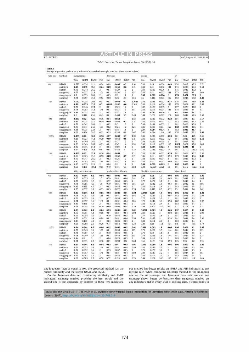
T.-T.-H. Phan et al. / Pattern Recognition Letters 0 0 0 (2017) 1–9 5
ARTICLE IN PRESS
JID: PATREC [m5G; August 30, 2017;13:44 ]
Table 2
Average imputation performance indexes of six methods on eight data sets (best results in bold).
Gap size Method Airpassenger Beersales Google SP
Sim NMAE RMSE FSD Sim NMAE RMSE FSD Sim NMAE RMSE FSD Sim NMAE RMSE FSD
6% DTWBI 0.777 0.034 21.1 0.24 0.88 0.035 0.7 0.14 0.83 0.14 0.034 0.43 0.74 0.026 35.5 0.7
na.interp 0.85 0.019 11.1 0.24 0.89 0.063 0.6 0.15 0.83 0.11 0.032 1.11 0.74 0.028 36.3 0.54
na.locf 0.76 0.044 26.3 2 0.81 0.129 1.2 2 0.81 0.126 0.036 2 0.75 0.022 29.2 2
na.approx 0.77 0.037 21.8 1.01 0.8 0.136 1.3 1.5 0.83 0.11 0.032 1.11 0.73 0.028 37 1.03
na.aggregate 0.8 0.033 20.1 2 0.83 0.11 1.1 2 0.86 0.082 0.024 2 0.78 0.021 26.5 2
na.spline 0.71 0.057 35.1 0.52 0.68 0.26 2.3 0.55 0.5 1.813 0.473 1.02 0.63 0.045 56.8 0.41
7.5% DTWBI 0.782 0.035 20.6 0.3 0.87 0.038 0.7 0.1629 0.84 0.131 0.032 0.33 0.76 0.03 38.9 0.52
na.interp 0.86 0.023 13.6 0.3 0.885 0.067 0.6 0.163 0.83 0.119 0.034 1.18 0.78 0.024 33.1 0.67
na.locf 0.77 0.046 27.4 2 0.81 0.123 1.2 2 0.82 0.126 0.035 2 0.77 0.026 34.8 2
na.approx 0.74 0.053 31.3 1.49 0.8 0.132 1.3 1.51 0.83 0.119 0.034 1.18 0.78 0.025 34 1.1
na.aggregate 0.81 0.033 20.2 2 0.82 0.112 1.1 2 0.87 0.081 0.024 2 0.8 0.022 29.1 2
na.spline 0.6 0.112 65.4 0.45 0.6 0.404 3.5 0.43 0.44 3.652 0.963 1.38 0.69 0.042 54.5 0.55
10% DTWBI 0.887 0.02 12.7 0.36 0.84 0.054 1 0.13 0.84 0.132 0.032 0.23 0.81 0.029 40.1 0.57
na.interp 0.86 0.021 13.1 0.34 0.89 0.068 0.7 0.18 0.85 0.105 0.03 1.22 0.82 0.025 36.3 0.56
na.locf 0.79 0.042 26.1 2 0.82 0.13 1.3 2 0.83 0.131 0.035 2 0.81 0.026 36.9 2
na.approx 0.79 0.041 24.6 1.03 0.82 0.124 1.2 1.24 0.85 0.105 0.03 1.22 0.83 0.024 33.5 1.14
na.aggregate 0.81 0.035 22.1 2 0.84 0.111 1.1 2 0.87 0.084 0.024 2 0.82 0.023 31.7 2
na.spline 0.62 0.134 78.3 0.52 0.55 0.558 4.9 0.67 0.42 4.684 1.118 1.13 0.76 0.049 63.2 0.45
12.5% DTWBI 0.893 0.02 12.6 0.36 0.87 0.039 0.7 0.12 0.85 0.138 0.032 0.23 0.8 0.03 41.9 0.61
na.interp 0.86 0.023 14.8 0.39 0.89 0.068 0.6 0.15 0.85 0.115 0.032 1.27 0.81 0.028 38.8 0.52
na.locf 0.8 0.044 26.9 2 0.82 0.127 1.2 2 0.84 0.129 0.035 2 0.81 0.027 36.1 2
na.approx 0.79 0.043 26.7 0.95 0.8 0.147 1.4 1.28 0.85 0.115 0.032 1.27 0.825 0.027 35.6 1.06
na.aggregate 0.82 0.035 21.8 2 0.84 0.109 1.1 2 0.88 0.083 0.024 2 0.824 0.024 31 2
na.spline 0.64 0.129 76.8 0.67 0.61 0.458 4 0.77 0.39 2.143 0.532 1.4 0.61 0.113 132.4 0.69
15% DTWBI 0.895 0.02 12.8 0.36 0.84 0.054 1 0.1 0.85 0.133 0.031 0.29 0.81 0.029 40.7 0.59
na.interp 0.86 0.025 15.6 0.35 0.89 0.069 0.7 0.17 0.86 0.11 0.031 0.99 0.79 0.033 43.6 0.49
na.locf 0.79 0.047 28.2 2 0.82 0.126 1.2 2 0.84 0.127 0.034 2 0.81 0.028 36.3 2
na.approx 0.8 0.043 26.5 1.17 0.83 0.117 1.1 1.42 0.86 0.11 0.031 0.99 0.81 0.032 41 1
na.aggregate 0.83 0.035 22.1 2 0.84 0.11 1.1 2 0.89 0.079 0.023 2 0.82 0.025 32 2
na.spline 0.55 0.175 106.1 0.95 0.49 0.731 6.3 0.88 0.34 12.339 2.928 1.6 0.61 0.136 162.5 0.68
CO 2 concentrations Mackey-Glass Chaotic Phu Lien temperature Water level
6% DTWBI 0.93 0.001 0.3 0.04 0.95 0.005 0.01 0.03 0.88 0.06 1.7 0.08 0.95 0.009 0.1 0.05
na.interp 0.75 0.055 1.6 1.5 0.79 0.031 0.04 0.81 0.8 0.142 3.1 0.63 0.81 0.042 0.5 1.05
na.locf 0.73 0.059 1.7 2 0.77 0.036 0.05 2 0.77 0.173 3.8 2 0.8 0.043 0.4 2
na.approx 0.75 0.055 1.6 1.5 0.79 0.031 0.04 0.81 0.8 0.142 3.1 0.63 0.81 0.042 0.5 1.05
na.aggregate 0.45 0.185 4.7 2 0.82 0.025 0.03 2 0.83 0.114 2.4 2 0.83 0.035 0.4 2
na.spline 0.75 0.057 1.6 0.75 0.65 0.072 0.09 0.38 0.61 0.413 8.5 0.52 0.3 0.654 6.6 1.61
7.5% DTWBI 0.93 0.001 0.4 0.05 0.93 0.008 0.01 0.02 0.8788 0.061 1.7 0.06 0.96 0.007 0.1 0.02
na.interp 0.74 0.057 1.6 1.38 0.8 0.031 0.04 1.04 0.79 0.147 3.2 0.98 0.82 0.038 0.4 0.97
na.locf 0.76 0.053 1.6 2 0.77 0.038 0.05 2 0.77 0.171 3.7 2 0.81 0.043 0.5 2
na.approx 0.74 0.057 1.6 1.38 0.8 0.031 0.04 1.04 0.79 0.147 3.2 0.98 0.82 0.038 0.4 0.97
na.aggregate 0.45 0.186 4.7 2 0.83 0.025 0.03 2 0.83 0.113 2.4 2 0.83 0.036 0.4 2
na.spline 0.74 0.058 1.6 0.79 0.69 0.062 0.08 0.39 0.58 0.701 14.5 0.8 0.2 1.228 12 1.71
10% DTWBI 0.93 0.001 0.4 0.04 0.93 0.008 0.01 0.01 0.8791 0.063 1.8 0.05 0.97 0.005 0.1 0.03
na.interp 0.76 0.051 1.4 0.88 0.81 0.03 0.04 0.98 0.81 0.137 3 0.58 0.81 0.041 0.4 0.91
na.locf 0.76 0.054 1.6 2 0.79 0.036 0.05 2 0.77 0.176 3.8 2 0.81 0.043 0.5 2
na.approx 0.76 0.051 1.4 0.88 0.81 0.03 0.04 0.98 0.81 0.137 3 0.58 0.81 0.041 0.4 0.91
na.aggregate 0.44 0.197 4.9 2 0.83 0.025 0.03 2 0.83 0.114 2.4 2 0.83 0.036 0.4 2
na.spline 0.66 0.098 2.9 0.26 0.71 0.058 0.08 0.33 0.49 0.88 17.8 1.04 0.18 1.57 15.5 1.79
12.5% DTWBI 0.94 0.001 0.3 0.04 0.92 0.009 0.02 0.01 0.881 0.065 1.8 0.04 0.96 0.006 0.1 0.03
na.interp 0.78 0.049 1.5 1.39 0.8 0.033 0.04 1.13 0.79 0.163 3.5 1.44 0.81 0.044 0.5 1.21
na.locf 0.75 0.057 1.7 2 0.79 0.036 0.05 2 0.78 0.18 3.8 2 0.81 0.043 0.5 2
na.approx 0.78 0.049 1.5 1.39 0.8 0.033 0.04 1.13 0.79 0.163 3.5 1.44 0.81 0.044 0.5 1.21
na.aggregate 0.44 0.2 5 2 0.84 0.025 0.03 2 0.84 0.116 2.4 2 0.83 0.036 0.4 2
na.spline 0.71 0.073 2.2 0.38 0.61 0.093 0.12 0.63 0.55 0.653 13.7 0.99 0.25 0.96 9.8 1.74
15% DTWBI 0.94 0.001 0.3 0.04 0.92 0.01 0.02 0.01 0.882 0.066 1.8 0.05 0.96 0.007 0.1 0.04
na.interp 0.76 0.053 1.6 1.46 0.81 0.03 0.04 0.99 0.81 0.145 3.2 1 0.81 0.044 0.5 1.6
na.locf 0.77 0.052 1.6 2 0.79 0.037 0.05 2 0.79 0.175 3.8 2 0.81 0.043 0.5 2
na.approx 0.76 0.053 1.6 1.46 0.81 0.03 0.04 0.99 0.81 0.145 3.2 1 0.81 0.044 0.5 1.6
na.aggregate 0.43 0.202 5.1 2 0.84 0.025 0.03 2 0.84 0.117 2.5 2 0.83 0.036 0.4 2
na.spline 0.69 0.085 2.5 0.58 0.57 0.129 0.16 0.73 0.44 1.268 26.3 1.27 0.21 1.185 11.8 1.83
size is greater than or equal to 10%, the proposed method has the
highest similarity and the lowest NMAE and RMSE.
On the Beersales data set, considering similarity and RMSE
indicators: na.interp method provides the best result and the
second one is our approach. By contrast to these two indicators,
our method has better results on NMEA and FSD indicators at any
missing rate. When comparing na.interp method to the na.approx
one on the Airpassenger and Beersales data sets, we can see
na.interp shows better performance than na.approx method on
any indicators and at every level of missing data. It corresponds to
Please cite this article as: T.-T.-H. Phan et al., Dynamic time warping-based imputation for univariate time series data, Pattern Recognition
Letters (2017), http://dx.doi.org/10.1016/j.patrec.2017.08.019
174
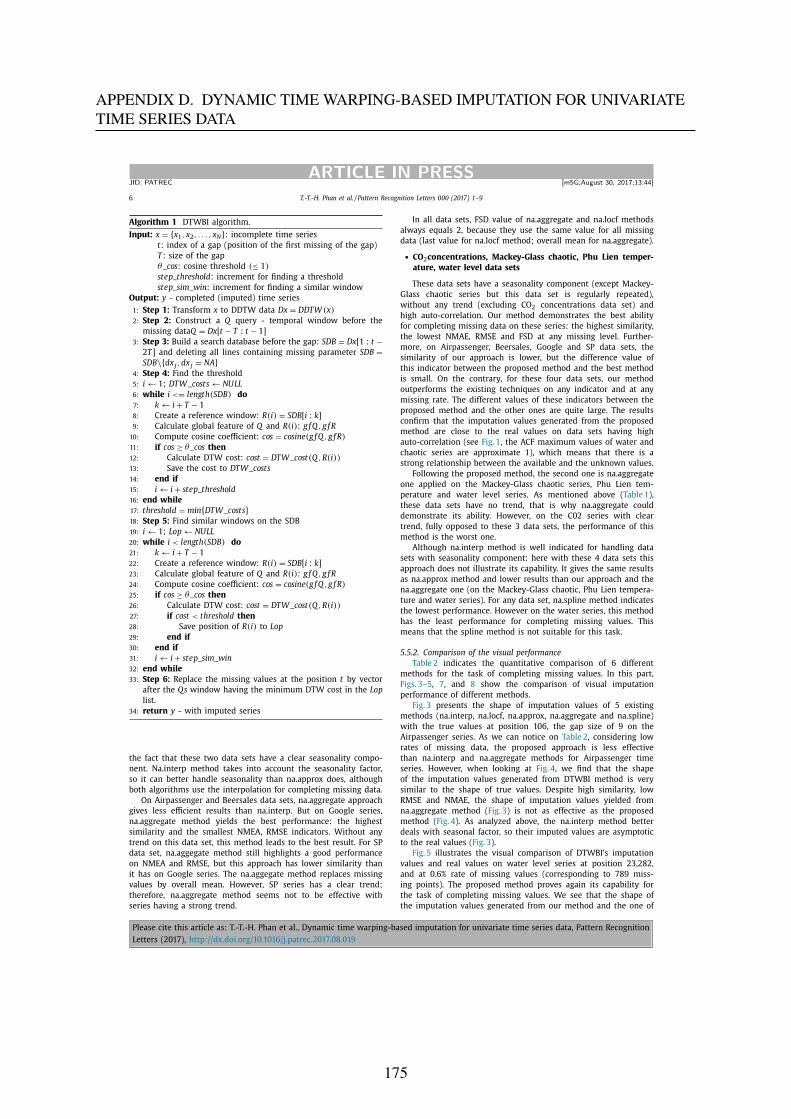
6 T.-T.-H. Phan et al. / Pattern Recognition Letters 0 0 0 (2017) 1–9
ARTICLE IN PRESS
JID: PATREC [m5G; August 30, 2017;13:44 ]
Algorithm 1 DTWBI algorithm.
Input: x = { x 1 , x 2 , . . . , x N } : incomplete time series
t: index of a gap (position of the first missing of the gap)
T : size of the gap
θ_ cos : cosine threshold (≤ 1)
step _ threshold: increment for finding a threshold
step _ sim _ win : increment for finding a similar window
Output: y - completed (imputed) time series
1: Step 1: Transform x to DDTW data Dx = DDT W (x )
2: Step 2: Construct a Q query - temporal window before the
missing data Q = Dx [ t − T : t − 1]
3: Step 3: Build a search database before the gap: SDB = Dx [1 : t −2 T ] and deleting all lines containing missing parameter SDB =
SDB \{ d x j , d x j = NA } 4: Step 4: Find the threshold
5: i ← 1 ; DT W _ costs ← NULL
6: while i < = length (SDB ) do
7: k ← i + T − 1
8: Create a reference window: R (i ) = SDB [ i : k ]
9: Calculate global feature of Q and R (i ) : g f Q, g f R
10: Compute cosine coefficient: cos = cosine (g f Q, g f R )
11: if cos ≥ θ_ cos then
12: Calculate DTW cost: cost = DT W _ cost(Q, R (i ))
13: Save the cost to DT W _ costs
14: end if
15: i ← i + step _ threshold
16: end while
17: threshold = min { DT W _ costs } 18: Step 5: Find similar windows on the SDB
19: i ← 1 ; Lop ← NULL
20: while i < length (SDB ) do
21: k ← i + T − 1
22: Create a reference window: R (i ) = SDB [ i : k ]
23: Calculate global feature of Q and R (i ) : g f Q, g f R
24: Compute cosine coefficient: cos = cosine (g f Q, g f R )
25: if cos ≥ θ_ cos then
26: Calculate DTW cost: cost = DT W _ cost(Q, R (i ))
27: if cost < threshold then
28: Save position of R (i ) to Lop
29: end if
30: end if
31: i ← i + step _ sim _ win
32: end while
33: Step 6: Replace the missing values at the position t by vector
after the Qs window having the minimum DTW cost in the Lop
list.
34: return y - with imputed series
the fact that these two data sets have a clear seasonality compo-
nent. Na.interp method takes into account the seasonality factor,
so it can better handle seasonality than na.approx does, although
both algorithms use the interpolation for completing missing data.
On Airpassenger and Beersales data sets, na.aggregate approach
gives less efficient results than na.interp. But on Google series,
na.aggregate method yields the best performance: the highest
similarity and the smallest NMEA, RMSE indicators. Without any
trend on this data set, this method leads to the best result. For SP
data set, na.aggegate method still highlights a good performance
on NMEA and RMSE, but this approach has lower similarity than
it has on Google series. The na.aggegate method replaces missing
values by overall mean. However, SP series has a clear trend;
therefore, na.aggregate method seems not to be effective with
series having a strong trend.
In all data sets, FSD value of na.aggregate and na.locf methods
always equals 2, because they use the same value for all missing
data (last value for na.locf method; overall mean for na.aggregate).
• CO 2 concentrations, Mackey-Glass chaotic, Phu Lien temper-
ature, water level data sets
These data sets have a seasonality component (except Mackey-
Glass chaotic series but this data set is regularly repeated),
without any trend (excluding CO 2 concentrations data set) and
high auto-correlation. Our method demonstrates the best ability
for completing missing data on these series: the highest similarity,
the lowest NMAE, RMSE and FSD at any missing level. Further-
more, on Airpassenger, Beersales, Google and SP data sets, the
similarity of our approach is lower, but the difference value of
this indicator between the proposed method and the best method
is small. On the contrary, for these four data sets, our method
outperforms the existing techniques on any indicator and at any
missing rate. The different values of these indicators between the
proposed method and the other ones are quite large. The results
confirm that the imputation values generated from the proposed
method are close to the real values on data sets having high
auto-correlation (see Fig. 1 , the ACF maximum values of water and
chaotic series are approximate 1), which means that there is a
strong relationship between the available and the unknown values.
Following the proposed method, the second one is na.aggregate
one applied on the Mackey-Glass chaotic series, Phu Lien tem-
perature and water level series. As mentioned above ( Table 1 ),
these data sets have no trend, that is why na.aggregate could
demonstrate its ability. However, on the C02 series with clear
trend, fully opposed to these 3 data sets, the performance of this
method is the worst one.
Although na.interp method is well indicated for handling data
sets with seasonality component: here with these 4 data sets this
approach does not illustrate its capability. It gives the same results
as na.approx method and lower results than our approach and the
na.aggregate one (on the Mackey-Glass chaotic, Phu Lien tempera-
ture and water series). For any data set, na.spline method indicates
the lowest performance. However on the water series, this method
has the least performance for completing missing values. This
means that the spline method is not suitable for this task.
5.5.2. Comparison of the visual performance
Table 2 indicates the quantitative comparison of 6 different
methods for the task of completing missing values. In this part,
Figs. 3–5 , 7 , and 8 show the comparison of visual imputation
performance of different methods.
Fig. 3 presents the shape of imputation values of 5 existing
methods (na.interp, na.locf, na.approx, na.aggregate and na.spline)
with the true values at position 106, the gap size of 9 on the
Airpassenger series. As we can notice on Table 2 , considering low
rates of missing data, the proposed approach is less effective
than na.interp and na.aggregate methods for Airpassenger time
series. However, when looking at Fig. 4 , we find that the shape
of the imputation values generated from DTWBI method is very
similar to the shape of true values. Despite high similarity, low
RMSE and NMAE, the shape of imputation values yielded from
na.aggregate method ( Fig. 3 ) is not as effective as the proposed
method ( Fig. 4 ). As analyzed above, the na.interp method better
deals with seasonal factor, so their imputed values are asymptotic
to the real values ( Fig. 3 ).
Fig. 5 illustrates the visual comparison of DTWBI’s imputation
values and real values on water level series at position 23,282,
and at 0.6% rate of missing values (corresponding to 789 miss-
ing points). The proposed method proves again its capability for
the task of completing missing values. We see that the shape of
the imputation values generated from our method and the one of
Please cite this article as: T.-T.-H. Phan et al., Dynamic time warping-based imputation for univariate time series data, Pattern Recognition
Letters (2017), http://dx.doi.org/10.1016/j.patrec.2017.08.019
APPENDIX D. DYNAMIC TIME WARPING-BASED IMPUTATION FOR UNIVARIATETIME SERIES DATA
175

T.-T.-H. Phan et al. / Pattern Recognition Letters 0 0 0 (2017) 1–9 7
ARTICLE IN PRESS
JID: PATREC [m5G; August 30, 2017;13:44 ]
Fig. 3. Visual comparison of imputed values of different imputation methods with
true values on Airpassenger series at position 106 with the gap size of 9.
Fig. 4. Visual comparison of imputed values of proposed method with true values
on Airpassenger series at position 106 with the gap size of 9.
the true values are almost completely identical. Fig. 6 shows the
matching pairs between the query and the most similar reference
window for the considered case. The values of matching pairs are
very close, which indicates the reason why the imputation values
generated from DTWBI are very similar to the real values. In con-
trast to our approach, handling seasonal factor of na.interp method
is ineffective on water level data set. This method does not pro-
vide good result such as on Airpassenger series ( Fig. 3 ); its perfor-
Fig. 5. Visual comparison of imputed values of the proposed method with true val-
ues on water level series at position 23,282 with the gap size of 789.
Fig. 6. Visual comparison of the query with the similar window on water level se-
ries at position 23,282 with the gap size of 789.
mance is the same as na.approx method ( Fig. 7 ). Fig. 8 especially
points out the obvious inefficiency of na.spline method for the task
of completing missing values, considering series with high auto-
correlation and large gap size (789 missing values in this case).
In this paper, we also calculate Cross-Correlation (CC) coeffi-
cients between the query with each reference window, and then
we find the maximum coefficient. CC demonstrates that a pattern
(here that is the query) exists or not in the database. High CC
value means that there exists the recurrence of the pattern in
the database. Therefore, we could easily find the pattern. Table 3
indicates the maximum of cross-correlation between the query
and reference windows.
Please cite this article as: T.-T.-H. Phan et al., Dynamic time warping-based imputation for univariate time series data, Pattern Recognition
Letters (2017), http://dx.doi.org/10.1016/j.patrec.2017.08.019
176
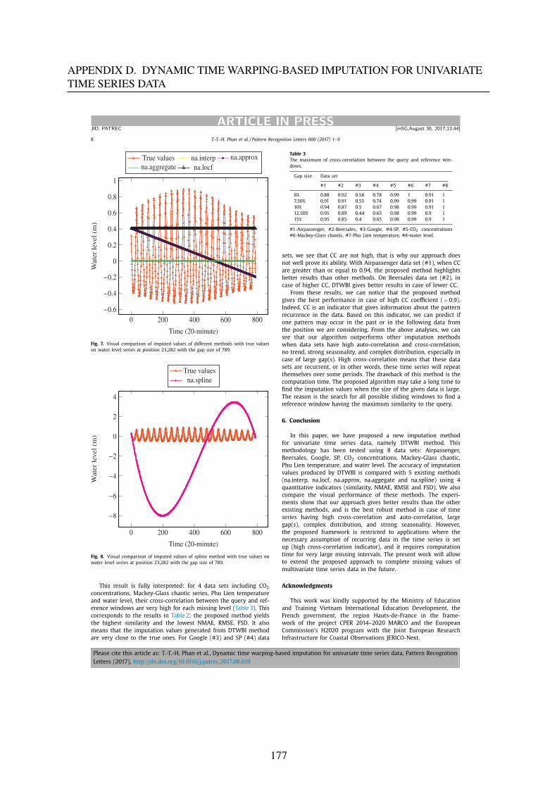
8 T.-T.-H. Phan et al. / Pattern Recognition Letters 0 0 0 (2017) 1–9
ARTICLE IN PRESS
JID: PATREC [m5G; August 30, 2017;13:44 ]
Fig. 7. Visual comparison of imputed values of different methods with true values
on water level series at position 23,282 with the gap size of 789.
Fig. 8. Visual comparison of imputed values of spline method with true values on
water level series at position 23,282 with the gap size of 789.
This result is fully interpreted: for 4 data sets including CO 2
concentrations, Mackey-Glass chaotic series, Phu Lien temperature
and water level, their cross-correlation between the query and ref-
erence windows are very high for each missing level ( Table 3 ). This
corresponds to the results in Table 2 : the proposed method yields
the highest similarity and the lowest NMAE, RMSE, FSD. It also
means that the imputation values generated from DTWBI method
are very close to the true ones. For Google (#3) and SP (#4) data
Table 3
The maximum of cross-correlation between the query and reference win-
dows.
Gap size Data set
#1 #2 #3 #4 #5 #6 #7 #8
6% 0.88 0.92 0.58 0.78 0.99 1 0.91 1
7.50% 0.91 0.91 0.55 0.74 0.99 0.99 0.91 1
10% 0.94 0.87 0.5 0.67 0.98 0.99 0.91 1
12.50% 0.95 0.89 0.44 0.65 0.98 0.99 0.9 1
15% 0.95 0.85 0.4 0.65 0.98 0.99 0.9 1
#1-Airpassenger, #2-Beersales, #3-Google, #4-SP, #5-CO 2 concentrations
#6-Mackey-Glass chaotic, #7-Phu Lien temperature, #8-water level.
sets, we see that CC are not high, that is why our approach does
not well prove its ability. With Airpassenger data set (#1), when CC
are greater than or equal to 0.94, the proposed method highlights
better results than other methods. On Beersales data set (#2), in
case of higher CC, DTWBI gives better results in case of lower CC.
From these results, we can notice that the proposed method
gives the best performance in case of high CC coefficient ( > 0.9).
Indeed, CC is an indicator that gives information about the pattern
recurrence in the data. Based on this indicator, we can predict if
one pattern may occur in the past or in the following data from
the position we are considering. From the above analyses, we can
see that our algorithm outperforms other imputation methods
when data sets have high auto-correlation and cross-correlation,
no trend, strong seasonality, and complex distribution, especially in
case of large gap(s). High cross-correlation means that these data
sets are recurrent, or in other words, these time series will repeat
themselves over some periods. The drawback of this method is the
computation time. The proposed algorithm may take a long time to
find the imputation values when the size of the given data is large.
The reason is the search for all possible sliding windows to find a
reference window having the maximum similarity to the query.
6. Conclusion
In this paper, we have proposed a new imputation method
for univariate time series data, namely DTWBI method. This
methodology has been tested using 8 data sets: Airpassenger,
Beersales, Google, SP, CO 2 concentrations, Mackey-Glass chaotic,
Phu Lien temperature, and water level. The accuracy of imputation
values produced by DTWBI is compared with 5 existing methods
(na.interp, na.locf, na.approx, na.aggegate and na.spline) using 4
quantitative indicators (similarity, NMAE, RMSE and FSD). We also
compare the visual performance of these methods. The experi-
ments show that our approach gives better results than the other
existing methods, and is the best robust method in case of time
series having high cross-correlation and auto-correlation, large
gap(s), complex distribution, and strong seasonality. However,
the proposed framework is restricted to applications where the
necessary assumption of recurring data in the time series is set
up (high cross-correlation indicator), and it requires computation
time for very large missing intervals. The present work will allow
to extend the proposed approach to complete missing values of
multivariate time series data in the future.
Acknowledgments
This work was kindly supported by the Ministry of Education
and Training Vietnam International Education Development, the
French government, the region Hauts-de-France in the frame-
work of the project CPER 2014–2020 MARCO and the European
Commission’s H2020 program with the Joint European Research
Infrastructure for Coastal Observations JERICO-Next.
Please cite this article as: T.-T.-H. Phan et al., Dynamic time warping-based imputation for univariate time series data, Pattern Recognition
Letters (2017), http://dx.doi.org/10.1016/j.patrec.2017.08.019
APPENDIX D. DYNAMIC TIME WARPING-BASED IMPUTATION FOR UNIVARIATETIME SERIES DATA
177
T.-T.-H. Phan et al. / Pattern Recognition Letters 0 0 0 (2017) 1–9 9
ARTICLE IN PRESS
JID: PATREC [m5G; August 30, 2017;13:44 ]
References
[1] P.D. Allison , Missing Data, Quantitative Applications in the Social Sciences, 136,
Sage Publication, 2001 .
[2] C.M. Bishop , Pattern Recognition and Machine Learning (Information Science and Statistics), Springer-Verlag New York, Inc., Secaucus, NJ, USA, 2006 .
[3] H.-T. Ceong , H.-J. Kim , J.-S. Park , Discovery of and recovery from failure in a costal marine usn service, J. Inf. Commun. Convergence Eng. 1 (1) (2012) .
[4] S. Chiewchanwattana , C. Lursinsap , C.-H. Henry Chu , Imputing incomplete time-series data based on varied-window similarity measure of data se-
quences, Pattern Recognit. Lett. 28 (9) (2007) 1091–1103 .
[5] S.L. Crawford , S.L. Tennstedt , J.B. McKinlay , A comparison of anlaytic methods for non-random missingness of outcome data, J. Clin. Epidemiol. 48 (2) (1995)
209–219 . [6] Y. Deng , C. Chang , M.S. Ido , Q. Long , Multiple imputation for general miss-
ing data patterns in the presence of high-dimensional data, Sci. Rep. 6 (2016) 21689 .
[7] A. Gelman, J. Hill, Y.-S. Su, M. Yajima, M. Pittau, B. Goodrich, Y. Si, J. Kropko, Mi: missing data imputation and model checking, 2015.
[8] M. Gómez-Carracedo , J. Andrade , P. López-Mahía , S. Muniategui , D. Prada , A
practical comparison of single and multiple imputation methods to handle complex missing data in air quality datasets, Chemometr. Intell. Lab. Syst. 134
(2014) 23–33 . [9] G. Hawthorne , P. Elliott , Imputing cross-sectional missing data: comparison of
common techniques, Aust. N. Z. J. Psychiatry 39 (7) (2005) 583–590 . [10] R. Hyndman , Y. Khandakar , Automatic time series forecasting: the forecast
package for r, used package in 2016, J. Stat. Softw. (2008) 1–22 .
[11] J.G. Joseph , A .A .E. El-Mohandes , M. Kiely , M.N. El-Khorazaty , M.G. Gantz , A .A . Johnson , K.S. Katz , S.M. Blake , M.W. Rossi , S. Subramanian , Reducing psy-
chosocial and behavioral pregnancy risk factors: results of a randomized clin- ical trial among high-risk pregnant African American women, Am. J. Public
Health 99 (6) (2009) 1053–1061 . [12] H. Junninen , H. Niska , K. Tuppurainen , J. Ruuskanen , M. Kolehmainen , Methods
for imputation of missing values in air quality data sets, Atmos. Environ. 38
(18) (2004) 2895–2907 . [13] E.J. Keogh , M.J. Pazzani , Derivative dynamic time warping., in: Sdm, 1, SIAM,
2001, pp. 5–7 . [14] K.J. Lee , J.B. Carlin , Multiple imputation for missing data: fully conditional
specification versus multivariate normal imputation, Am. J. Epidemiol. 171 (5) (2010) 624–632 .
[15] A. Lefebvre, MAREL Carnot data and metadata from Coriolis data centre. SEA-
NOE. http://doi.org/10.17882/39754 , 2015. [16] S.G. Liao , Y. Lin , D.D. Kang , D. Chandra , J. Bon , N. Kaminski , F.C. Sciurba ,
G.C. Tseng , Missing value imputation in high-dimensional phenomic data: im- putable or not, and how? BMC Bioinform. 15 (2014) 346 .
[17] R.J.A. Little , D.B. Rubin , Statistical Analysis with Missing Data, John Wiley & Sons, 2014 . Google-Books-ID: AyVeBAAAQBAJ.
[18] M.C. Mackey , L. Glass , Oscillation and Chaos in Physiological Control Systems,
197, Science (New York, N.Y.), 1977, pp. 287–289 . [19] S. Moritz, A. Sardá, T. Bartz-Beielstein, M. Zaefferer, J. Stork, Comparison of
different methods for univariate time series imputation in r, arXiv preprint arXiv:1510.03924 (2015).
[20] N.M. Noor , M.M. Al Bakri Abdullah , A.S. Yahaya , N.A. Ramli , Comparison of lin- ear interpolation method and mean method to replace the missing values in
environmental data set, Mater. Sci. Forum 803 (2014) 278–281 . [21] T.T.H. Phan , E.P. Caillault , A. Bigand , Comparative study on supervised learn-
ing methods for identifying phytoplankton species, in: 2016 IEEE Sixth In- ternational Conference on Communications and Electronics (ICCE), IEEE, 2016,
pp. 283–288 .
[22] R Core Team, R: A Language and Environment for Statistical Computing, R Foundation for Statistical Computing, Vienna, Austria, 2016.
[23] T.E. Raghunathan , J.M. Lepkowski , J. Van Hoewyk , P. Solenberger , A multivariate technique for multiply imputing missing values using a sequence of regression
models, Surv. Methodol. 27 (1) (2001) 85–96 . [24] T.E. Raghunathan , D.S. Siscovick , A multiple-imputation analysis of a case–
control study of the risk of primary cardiac arrest among pharmacologically
treated hypertensives on JSTOR, R. Stat. Soc.. Ser. C (Appl. Stat.) 45 (1996) 335–352 .
[25] S.A. Rahman , Y. Huang , J. Claassen , N. Heintzman , S. Kleinberg , Combining Fourier and lagged k-nearest neighbor imputation for biomedical time series
data, J. Biomed. Inform. 58 (2015) 198–207 . [26] K. Rousseeuw , E.P. Caillault , A. Lefebvre , D. Hamad , Monitoring system of phy-
toplankton blooms by using unsupervised classifier and time modeling, in:
2013 IEEE International Geoscience and Remote Sensing Symposium-IGARSS, IEEE, 2013, pp. 3962–3965 .
[27] P. Royston , Multiple imputation of missing values: further update of ice, with an emphasis on interval censoring, Stata J. 7 (4) (2007) 445–464 .
[28] H. Sakoe , S. Chiba , Dynamic programming algorithm optimization for spoken word recognition, IEEE Trans. Acoust., Speech, Signal Process. 16 (1978) 43–49 .
[29] J. Schafer , Analysis of Incomplete Multivariate Data, Chapman and Hall, Lon-
don, 1997 . [30] A.D. Shah , J.W. Bartlett , J. Carpenter , O. Nicholas , H. Hemingway , Comparison
of random forest and parametric imputation models for imputing missing data using MICE: a CALIBER study, Am. J. Epidemiol. 179 (6) (2014) 764–774 .
[31] M. Spratt , J. Carpenter , J.A.C. Sterne , J.B. Carlin , J. Heron , J. Henderson , K. Tilling , Strategies for multiple imputation in longitudinal studies, Am. J. Epidemiol. 172
(4) (2010) 478–487 .
[32] J.A.C. Sterne , I.R. White , J.B. Carlin , M. Spratt , P. Royston , M.G. Kenward , A.M. Wood , J.R. Carpenter , Multiple imputation for missing data in epidemi-
ological and clinical research: potential and pitfalls, BMJ (Clin. Resear. ed.) 338 (2009) b2393 .
[33] E.A. Stuart , M. Azur , C. Frangakis , P. Leaf , Multiple imputation with large data sets: a case study of the children’s mental health initiative, Am. J. Epidemiol.
169 (9) (2009) 1133–1139 . [34] K.W. Thoning , P.P. Tans , W.D. Komhyr , Atmospheric carbon dioxide at mauna
loa observatory. II - analysis of the NOAA GMCC data, 1974–1985 94 (1989)
8549–8565 . [35] S. Van Buuren , H.C. Boshuizen , D.L. Knook , others , Multiple imputation of miss-
ing blood pressure covariates in survival analysis, Stat. Med. 18 (6) (1999) 681–694 .
[36] Y. Walter.O , J.M. Kihoro , K.H.O. Athiany , K.H. W , Imputation of incomplete non- stationary seasonal time series data, Math. Theory Model. 3 (12) (2013)
142–154 .
[37] A. Zeileis, G. Grothendieck, zoo: S3 infrastructure for regular and irregular time series, used package in 2016, 2005, doi: 10.18637/jss.v014.i06 .
Please cite this article as: T.-T.-H. Phan et al., Dynamic time warping-based imputation for univariate time series data, Pattern Recognition
Letters (2017), http://dx.doi.org/10.1016/j.patrec.2017.08.019
178
Bibliography
[1] K. Rousseeuw, É P. Caillault, A. Lefebvre, and D. Hamad. Monitoring system of phy-
toplankton blooms by using unsupervised classifier and time modeling. In 2013 IEEE
International Geoscience and Remote Sensing Symposium - IGARSS, pages 3962–3965,
July 2013.
[2] Hee-Taek Ceong, Hae-Jin Kim, and Jeong-Seon Park. Discovery of and recovery from
failure in a costal marine usn service. Journal of Information and Communication Con-
vergence Engineering, 1(1), Mar 2012.
[3] Alain Lefebvre. MAREL Carnot data and metadata from Coriolis Data Centre. SEA-
NOE. http://doi.org/10.17882/39754, 2015.
[4] Graeme Hawthorne and Peter Elliott. Imputing cross-sectional missing data: Compar-
ison of common techniques. The Australian and New Zealand Journal of Psychiatry,
39(7):583–590, July 2005.
[5] Heikki Junninen, Harri Niska, Kari Tuppurainen, Juhani Ruuskanen, and Mikko
Kolehmainen. Methods for imputation of missing values in air quality data sets. At-
mospheric Environment, 38(18):2895–2907, June 2004.
[6] Tommy D. Dickey. Emerging ocean observations for interdisciplinary data assimilation
systems. Journal of Marine Systems, 40-41:5–48, April 2003.
[7] Hiroaki Sakoe and Seibi Chiba. Dynamic Programming Algorithm Optimization for
Spoken Word Recognition. IEEE transactions on acoustics, speech, and signal process-
ing, 16:43–49, 1978.
179
[8] Eamonn J. Keogh and Michael J. Pazzani. Scaling up dynamic time warping for datamin-
ing applications. In Proceedings of the sixth ACM SIGKDD international conference on
Knowledge discovery and data mining, pages 285–289. ACM, 2000.
[9] Donald J. Berndt and James Clifford. Using dynamic time warping to find patterns in
time series. In Proceedings of the 3rd International Conference on Knowledge Discovery
and Data Mining, AAAIWS’94, pages 359–370. AAAI Press, 1994.
[10] Y. Jeong, M. K. Jeong, and O. A. Omitaomu. Weighted dynamic time warping for time
series classification. Pattern Recognition, 44(9):2231–2240, September 2011.
[11] Harold Mouchère, Jinpeng Li, Christian Viard-Gaudin, and Zhaoxin Chen. A dynamic
Time Warping Algorithm for Recognition of Multi-Stroke On-Line Handwriten Char-
acters. Natural Science Edition, Journal of South China University of Technology,
41(7):pp. 107–113, June 2013.
[12] Toni M. Rath and R. Manmatha. Word image matching using dynamic time warping. In
CVPR (2), pages 521–527. IEEE Computer Society, 2003.
[13] Xiaopeng Xi, Eamonn Keogh, Christian Shelton, Li Wei, and Chotirat Ann Ratanama-
hatana. Fast time series classification using numerosity reduction. pages 1033–1040.
ACM Press, 2006.
[14] François Petitjean, Alain Ketterlin, and Pierre Gançarski. A global averaging method for
dynamic time warping, with applications to clustering. Pattern Recognition, 44(3):678–
693, March 2011.
[15] Y. Gupta, A. Saini, and A. Saxena. Fuzzy logic-based approach to develop hybrid
similarity measure for efficient information retrieval. Journal of Information Science,
40(6):846–857, December 2014.
[16] Shyi-Ming Chen, Ming-Shiow Yeh, and Pei-Yung Hsiao. A comparison of similarity
measures of fuzzy values. Fuzzy Sets and Systems, 72(1):79–89, May 1995.
[17] Mohammad Yahya H. Al-Shamri and Nagi H. Al-Ashwal. Fuzzy-Weighted Similarity
Measures for Memory-Based Collaborative Recommender Systems. Journal of Intelli-
gent Learning Systems and Applications, 06(01):1–10, 2014.
180
[18] Parivash Pirasteh, Dosam Hwang, and Jai E. Jung. Weighted Similarity Schemes for
High Scalability in User-Based Collaborative Filtering. Mobile Netw Appl, 20(4):497–
507, August 2015.
[19] Yong Wang, Jiangzhou Deng, Jerry Gao, and Pu Zhang. A hybrid user similarity model
for collaborative filtering. Information Sciences, 418(Supplement C):102–118, Decem-
ber 2017.
[20] Sina Shahmoradi and Saeed Bagheri Shouraki. Evaluation of a novel fuzzy sequential
pattern recognition tool (fuzzy elastic matching machine) and its applications in speech
and handwriting recognition. Applied Soft Computing, 62:315–327, January 2018.
[21] Plamen P. Angelov and Dimitar Filev. Flexible models with evolving structure. Int. J.
Intell. Syst., 19(4):327–340, 2004.
[22] P. Angelov and R. Buswell. Identification of evolving fuzzy rule-based models. IEEE
Transactions on Fuzzy Systems, 10(5):667–677, October 2002.
[23] Plamen P. Angelov and Ronald R. Yager. A new type of simplified fuzzy rule-based
system. Int. J. General Systems, 41(2):163–185, 2012.
[24] Chao-Chih Tsai and Ke-Chih Chen. An application of fuzzy rule-based system: to the
economic equilibrium considering the shift in demand curve. In Proceedings Joint 9th
IFSA World Congress and 20th NAFIPS International Conference (Cat. No. 01TH8569),
pages 2608–2611 vol.5, July 2001.
[25] Roderick J. A. Little and Donald B. Rubin. Statistical Analysis with Missing Data. John
Wiley & Sons, August 2014. Google-Books-ID: AyVeBAAAQBAJ.
[26] Yiran Dong and Joanne Peng. Principled missing data methods for researchers. Springer-
Plus, 2:222, 12 2013.
[27] Steffen Moritz, Alexis Sardá, Thomas Bartz-Beielstein, Martin Zaefferer, and Jörg Stork.
Comparison of different Methods for Univariate Time Series Imputation in R. arXiv
preprint arXiv:1510.03924, 2015.
[28] M.P. Gómez-Carracedo, J.M. Andrade, P. López-Mahía, S. Muniategui, and D. Prada.
A practical comparison of single and multiple imputation methods to handle complex
181
missing data in air quality datasets. Chemometrics and Intelligent Laboratory Systems,
134:23–33, May 2014.
[29] Geert Molenberghs, Garrett Fitzmaurice, Michael G. Kenward, Geert Verbeke, and
Anastasios Tsiatis. Handbook of missing data methodology. CRC Press, 2014.
[30] Alain Lefebvre. MAREL Carnot data and metadata from Coriolis Data Centre. SEA-
NOE. http://doi.org/10.17882/39754, 2015.
[31] R Core Team. R: A Language and Environment for Statistical Computing. R Foundation
for Statistical Computing, Vienna, Austria, 2016.
[32] D. Woehrling, A. Lefebvre, and R. Le Fèvre-Lehoërff, G.and Delesmont. Seasonal and
longer term trends in sea temperature along the french north sea coast, 1975 to 2002.
Journal of the Marine Biological Association U.K., 85 (1), pages 39–48, 2005.
[33] Chris Chatfield. The Analysis of Time Series: An Introduction, Sixth Edition. CRC Press,
March 2016.
[34] Norman R. Draper and Harry Smith. Applied Regression Analysis. Wiley, April 1998.
[35] P. Grosjean and F. Ibanez. PASTECS. Manuel de l’utilisateur de la librairie de fonctions
pour R et pour S+ Package for Analysis of Space-Time Ecological Series, 2002.
[36] Norazian Mohamed Noor, Mohd Mustafa Al Bakri Abdullah, Ahmad Shukri Yahaya,
and Nor Azam Ramli. Comparison of Linear Interpolation Method and Mean Method
to Replace the Missing Values in Environmental Data Set. Materials Science Forum,
803:278–281, August 2014.
[37] Paul D. Allison. Missing Data, volume 136 of Quantitative Applications in the Social
Sciences. Sage Publication, 2001.
[38] Christopher M. Bishop. Pattern Recognition and Machine Learning (Information Sci-
ence and Statistics). Springer-Verlag New York, Inc., Secaucus, NJ, USA, 2006.
[39] S. L. Crawford, S. L. Tennstedt, and J. B. McKinlay. A comparison of anlaytic meth-
ods for non-random missingness of outcome data. Journal of Clinical Epidemiology,
48(2):209–219, February 1995.
182
[40] Jonathan A. C. Sterne, Ian R. White, John B. Carlin, Michael Spratt, Patrick Royston,
Michael G. Kenward, Angela M. Wood, and James R. Carpenter. Multiple imputation
for missing data in epidemiological and clinical research: Potential and pitfalls. BMJ
(Clinical research ed.), 338:b2393, 2009.
[41] Yodah Walter.O, J. M. Kihoro, K. H. O. Athiany, and Kibunja H. W. Imputation of in-
complete non- stationary seasonal time series data. Mathematical Theory and Modeling,
3(12):142–154, 2013.
[42] Sirapat Chiewchanwattana, Chidchanok Lursinsap, and Chee-Hung Henry Chu. Im-
puting incomplete time-series data based on varied-window similarity measure of data
sequences. Pattern Recognition Letters, 28(9):1091–1103, July 2007.
[43] Ilaria Bartolini, Paolo Ciaccia, and Marco Patella. Warp: Accurate retrieval of shapes
using phase of fourier descriptors and time warping distance. IEEE transactions on
pattern analysis and machine intelligence, 27(1):142–147, 2005.
[44] Andrés Marzal, Vicente Palazón, and Guillermo Peris. Contour-Based Shape Retrieval
Using Dynamic Time Warping. In Current Topics in Artificial Intelligence, Lecture
Notes in Computer Science, pages 190–199. Springer, Berlin, Heidelberg, November
2005.
[45] J. Aach and G. M. Church. Aligning gene expression time series with time warping
algorithms. Bioinformatics (Oxford, England), 17(6):495–508, June 2001.
[46] GenTXWarper - Dynamic Time Warping algorithm for gene expression time series. [On-
line]. Available: http://www.psb.ugent.be/cbd/papers/gentxwarper/DTWalgorithm.htm.
[47] F. Itakura. Minimum prediction residual principle applied to speech recognition. IEEE
Transactions on Acoustics, Speech, and Signal Processing, 23(1):67–72, February 1975.
[48] Eamonn J. Keogh and Michael J. Pazzani. Derivative dynamic time warping. In Proceed-
ings of the 2001 SIAM International Conference on Data Mining, pages 1–11. SIAM,
2001.
[49] Xie Ying and Wiltgen Bryan. Adaptive Feature Based Dynamic Time Warping. IJCSNS
International Journal of Computer Science and Network Security, 10:264–273, January
2010.
183
[50] Émilie Caillault, Pierre-Alexandre Hébert, and Guillaume Wacquet. Dissimilarity-Based
Classification of Multidimensional Signals by Conjoint Elastic Matching: Application to
Phytoplanktonic Species Recognition. In Engineering Applications of Neural Networks,
number 43 in Communications in Computer and Information Science, pages 153–164.
Springer Berlin Heidelberg, 2009-08-27.
[51] Yanping Chen, Bing Hu, Eamonn Keogh, and Gustavo EAPA Batista. DTW-D: Time
series semi-supervised learning from a single example. In Proceedings of the 19th ACM
SIGKDD International Conference on Knowledge Discovery and Data Mining, pages
383–391. ACM, 2013.
[52] T. T. H. Phan, E. P. Caillault, and A. Bigand. Comparative study on supervised learning
methods for identifying phytoplankton species. In 2016 IEEE Sixth International Con-
ference on Communications and Electronics (ICCE), pages 283–288. IEEE, July 2016.
[53] RJ Hyndman and Y Khandakar. Automatic time series forecasting: the forecast package
for r, used package in 2016. Journal of Statistical Software, pages 1–22, September
2008.
[54] Kirk W Thoning, Pieter P Tans, and Walter D Komhyr. Atmospheric carbon dioxide at
Mauna Loa Observatory. II - Analysis of the NOAA GMCC data, 1974-1985. Journal
of Geophysical Research-Atmospheres, 94:8549–8565, June 1989.
[55] M. C. Mackey and L. Glass. Oscillation and chaos in physiological control systems.
Science (New York, N.Y.), 197(4300):287–289, July 1977.
[56] Achim Zeileis and Gabor Grothendieck. zoo: S3 infrastructure for regular and irregular
time series. Journal of Statistical Software, 14(6):1–27, 2005.
[57] David L. Streiner. Missing data and the trouble with LOCF. Evidence-Based Mental
Health, 11(1):3–5, February 2008.
[58] Geert Molenberghs, Herbert Thijs, Ivy Jansen, Caroline Beunckens, Michael G. Ken-
ward, Craig Mallinckrodt, and Raymond J. Carroll. Analyzing incomplete longitudinal
clinical trial data. Biostatistics (Oxford, England), 5(3):445–464, July 2004.
[59] Hui-Huang Hsu, Andy C. Yang, and Ming-Da Lu. KNN-DTW Based Missing Value
Imputation for Microarray Time Series Data. Journal of Computers, 6(3), March 2011.
184
[60] Stefan Oehmcke, Oliver Zielinski, and Oliver Kramer. kNN ensembles with penalized
DTW for multivariate time series imputation. In Neural Networks (IJCNN), 2016 Inter-
national Joint Conference On, pages 2774–2781. IEEE, 2016.
[61] Elena Kostadinova, Veselka Boeva, Liliana Boneva, and Elena Tsiporkova. An Integra-
tive DTW-based imputation method for gene expression time series data. In Intelligent
Systems (IS), 2012 6th IEEE International Conference, pages 258–263. IEEE, 2012.
[62] Andy C. Yang, Hui-Huang Hsu, and Ming-Da Lu. Missing Value Imputation in Microar-
ray Gene Expression Data. In Conference on Information Technology and Applications
in Outlying Islands, 2009.
[63] US Energy Information Administration. Product Supplied for Finished Gaso-
line. http://www.eia.gov/dnav/pet/PET_SUM_SNDW_A_EPM0F_VPP_MBBLPD_W.
htm, 2016. gas_online_product_2016.
[64] J.L. Schafer. Analysis of Incomplete Multivariate Data. Chapman and Hall, London,
1997.
[65] Stef Van Buuren, Hendriek C. Boshuizen, Dick L. Knook, and others. Multiple impu-
tation of missing blood pressure covariates in survival analysis. Statistics in medicine,
18(6):681–694, 1999.
[66] Trivellore E. Raghunathan, James M. Lepkowski, John Van Hoewyk, and Peter Solen-
berger. A multivariate technique for multiply imputing missing values using a sequence
of regression models. Survey methodology, 27(1):85–96, 2001.
[67] J Engels and Paula Diehr. Imputation of missing longitudinal data: A comparison of
methods. Journal of Clinical Epidemiology, 56(10):968–976, October 2003.
[68] Patrick Royston. Multiple imputation of missing values: Further update of ice, with an
emphasis on interval censoring. Stata Journal, 7(4):445–464, 2007.
[69] Elizabeth A. Stuart, Melissa Azur, Constantine Frangakis, and Philip Leaf. Multiple Im-
putation With Large Data Sets: A Case Study of the Children’s Mental Health Initiative.
American Journal of Epidemiology, 169(9):1133–1139, May 2009.
185
[70] Katherine J. Lee and John B. Carlin. Multiple Imputation for Missing Data: Fully Con-
ditional Specification Versus Multivariate Normal Imputation. American Journal of Epi-
demiology, 171(5):624–632, March 2010.
[71] Anoop D. Shah, Jonathan W. Bartlett, James Carpenter, Owen Nicholas, and Harry Hem-
ingway. Comparison of random forest and parametric imputation models for imput-
ing missing data using MICE: A CALIBER study. American Journal of Epidemiology,
179(6):764–774, March 2014.
[72] Serena G. Liao, Yan Lin, Dongwan D. Kang, Divay Chandra, Jessica Bon, Naftali
Kaminski, Frank C. Sciurba, and George C. Tseng. Missing value imputation in high-
dimensional phenomic data: Imputable or not, and how? BMC Bioinformatics, 15:346,
2014.
[73] Shah Atiqur Rahman, Yuxiao Huang, Jan Claassen, Nathaniel Heintzman, and Samantha
Kleinberg. Combining Fourier and lagged k -nearest neighbor imputation for biomedical
time series data. Journal of Biomedical Informatics, 58:198–207, December 2015.
[74] Andrew Gelman, Jennifer Hill, Yu-Sung Su, Masanao Yajima, Maria Pittau, Ben
Goodrich, Yajuan Si, and Jon Kropko. Mi: Missing Data Imputation and Model Check-
ing, April 2015.
[75] Yi Deng, Changgee Chang, Moges Seyoum Ido, and Qi Long. Multiple Imputation
for General Missing Data Patterns in the Presence of High-dimensional Data. Scientific
Reports, 6:21689, February 2016.
[76] Daniel J. Stekhoven and Peter Bühlmann. MissForest—non-parametric missing value
imputation for mixed-type data. Bioinformatics, 28(1):112–118, 2012.
[77] Piero Bonissone, José M. Cadenas, M. Carmen Garrido, and R. Andrés Díaz-Valladares.
A fuzzy random forest. International Journal of Approximate Reasoning, 51(7):729–
747, September 2010.
[78] Shah Atiqur Rahman, Yuxiao Huang, Jan Claassen, Nathaniel Heintzman, and Samantha
Kleinberg. Combining Fourier and lagged k -nearest neighbor imputation for biomedical
time series data. Journal of Biomedical Informatics, 58:198–207, December 2015.
186
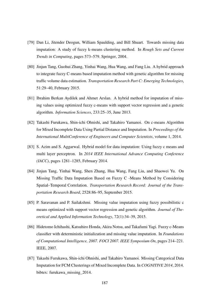
[79] Dan Li, Jitender Deogun, William Spaulding, and Bill Shuart. Towards missing data
imputation: A study of fuzzy k-means clustering method. In Rough Sets and Current
Trends in Computing, pages 573–579. Springer, 2004.
[80] Jinjun Tang, Guohui Zhang, Yinhai Wang, Hua Wang, and Fang Liu. A hybrid approach
to integrate fuzzy C-means based imputation method with genetic algorithm for missing
traffic volume data estimation. Transportation Research Part C: Emerging Technologies,
51:29–40, February 2015.
[81] Ibrahim Berkan Aydilek and Ahmet Arslan. A hybrid method for imputation of miss-
ing values using optimized fuzzy c-means with support vector regression and a genetic
algorithm. Information Sciences, 233:25–35, June 2013.
[82] Takashi Furukawa, Shin-ichi Ohnishi, and Takahiro Yamanoi. On c-means Algorithm
for Mixed Incomplete Data Using Partial Distance and Imputation. In Proceedings of the
International MultiConference of Engineers and Computer Scientists, volume 1, 2014.
[83] S. Azim and S. Aggarwal. Hybrid model for data imputation: Using fuzzy c means and
multi layer perceptron. In 2014 IEEE International Advance Computing Conference
(IACC), pages 1281–1285, February 2014.
[84] Jinjun Tang, Yinhai Wang, Shen Zhang, Hua Wang, Fang Liu, and Shaowei Yu. On
Missing Traffic Data Imputation Based on Fuzzy C -Means Method by Considering
Spatial–Temporal Correlation. Transportation Research Record: Journal of the Trans-
portation Research Board, 2528:86–95, September 2015.
[85] P. Saravanan and P. Sailakshmi. Missing value imputation using fuzzy possibilistic c
means optimized with support vector regression and genetic algorithm. Journal of The-
oretical and Applied Information Technology, 72(1):34–39, 2015.
[86] Hidetomo Ichihashi, Katsuhiro Honda, Akira Notsu, and Takafumi Yagi. Fuzzy c-Means
classifier with deterministic initialization and missing value imputation. In Foundations
of Computational Intelligence, 2007. FOCI 2007. IEEE Symposium On, pages 214–221.
IEEE, 2007.
[87] Takashi Furukawa, Shin-ichi Ohnishi, and Takahiro Yamanoi. Missing Categorical Data
Imputation for FCM Clusterings of Mixed Incomplete Data. In COGNITIVE 2014, 2014.
bibtex: furukawa_missing_2014.
187
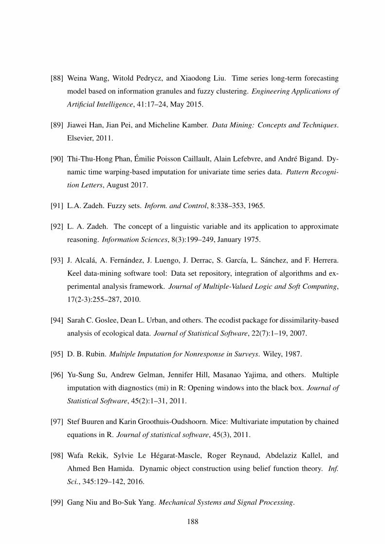
[88] Weina Wang, Witold Pedrycz, and Xiaodong Liu. Time series long-term forecasting
model based on information granules and fuzzy clustering. Engineering Applications of
Artificial Intelligence, 41:17–24, May 2015.
[89] Jiawei Han, Jian Pei, and Micheline Kamber. Data Mining: Concepts and Techniques.
Elsevier, 2011.
[90] Thi-Thu-Hong Phan, Émilie Poisson Caillault, Alain Lefebvre, and André Bigand. Dy-
namic time warping-based imputation for univariate time series data. Pattern Recogni-
tion Letters, August 2017.
[91] L.A. Zadeh. Fuzzy sets. Inform. and Control, 8:338–353, 1965.
[92] L. A. Zadeh. The concept of a linguistic variable and its application to approximate
reasoning. Information Sciences, 8(3):199–249, January 1975.
[93] J. Alcalá, A. Fernández, J. Luengo, J. Derrac, S. García, L. Sánchez, and F. Herrera.
Keel data-mining software tool: Data set repository, integration of algorithms and ex-
perimental analysis framework. Journal of Multiple-Valued Logic and Soft Computing,
17(2-3):255–287, 2010.
[94] Sarah C. Goslee, Dean L. Urban, and others. The ecodist package for dissimilarity-based
analysis of ecological data. Journal of Statistical Software, 22(7):1–19, 2007.
[95] D. B. Rubin. Multiple Imputation for Nonresponse in Surveys. Wiley, 1987.
[96] Yu-Sung Su, Andrew Gelman, Jennifer Hill, Masanao Yajima, and others. Multiple
imputation with diagnostics (mi) in R: Opening windows into the black box. Journal of
Statistical Software, 45(2):1–31, 2011.
[97] Stef Buuren and Karin Groothuis-Oudshoorn. Mice: Multivariate imputation by chained
equations in R. Journal of statistical software, 45(3), 2011.
[98] Wafa Rekik, Sylvie Le Hégarat-Mascle, Roger Reynaud, Abdelaziz Kallel, and
Ahmed Ben Hamida. Dynamic object construction using belief function theory. Inf.
Sci., 345:129–142, 2016.
[99] Gang Niu and Bo-Suk Yang. Mechanical Systems and Signal Processing.
188
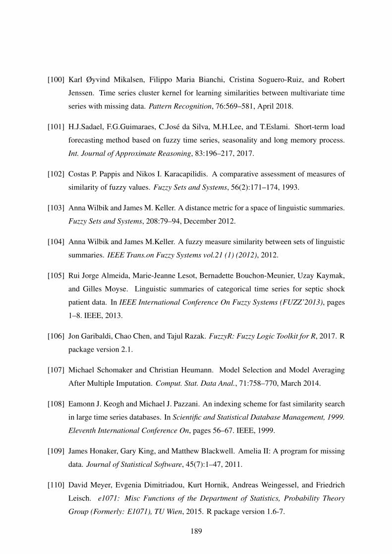
[100] Karl Øyvind Mikalsen, Filippo Maria Bianchi, Cristina Soguero-Ruiz, and Robert
Jenssen. Time series cluster kernel for learning similarities between multivariate time
series with missing data. Pattern Recognition, 76:569–581, April 2018.
[101] H.J.Sadael, F.G.Guimaraes, C.José da Silva, M.H.Lee, and T.Eslami. Short-term load
forecasting method based on fuzzy time series, seasonality and long memory process.
Int. Journal of Approximate Reasoning, 83:196–217, 2017.
[102] Costas P. Pappis and Nikos I. Karacapilidis. A comparative assessment of measures of
similarity of fuzzy values. Fuzzy Sets and Systems, 56(2):171–174, 1993.
[103] Anna Wilbik and James M. Keller. A distance metric for a space of linguistic summaries.
Fuzzy Sets and Systems, 208:79–94, December 2012.
[104] Anna Wilbik and James M.Keller. A fuzzy measure similarity between sets of linguistic
summaries. IEEE Trans.on Fuzzy Systems vol.21 (1) (2012), 2012.
[105] Rui Jorge Almeida, Marie-Jeanne Lesot, Bernadette Bouchon-Meunier, Uzay Kaymak,
and Gilles Moyse. Linguistic summaries of categorical time series for septic shock
patient data. In IEEE International Conference On Fuzzy Systems (FUZZ’2013), pages
1–8. IEEE, 2013.
[106] Jon Garibaldi, Chao Chen, and Tajul Razak. FuzzyR: Fuzzy Logic Toolkit for R, 2017. R
package version 2.1.
[107] Michael Schomaker and Christian Heumann. Model Selection and Model Averaging
After Multiple Imputation. Comput. Stat. Data Anal., 71:758–770, March 2014.
[108] Eamonn J. Keogh and Michael J. Pazzani. An indexing scheme for fast similarity search
in large time series databases. In Scientific and Statistical Database Management, 1999.
Eleventh International Conference On, pages 56–67. IEEE, 1999.
[109] James Honaker, Gary King, and Matthew Blackwell. Amelia II: A program for missing
data. Journal of Statistical Software, 45(7):1–47, 2011.
[110] David Meyer, Evgenia Dimitriadou, Kurt Hornik, Andreas Weingessel, and Friedrich
Leisch. e1071: Misc Functions of the Department of Statistics, Probability Theory
Group (Formerly: E1071), TU Wien, 2015. R package version 1.6-7.
189
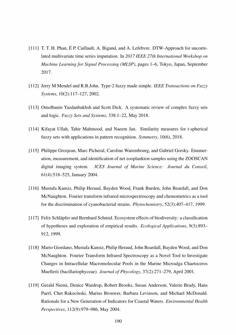
[111] T. T. H. Phan, É P. Caillault, A. Bigand, and A. Lefebvre. DTW-Approach for uncorre-
lated multivariate time series imputation. In 2017 IEEE 27th International Workshop on
Machine Learning for Signal Processing (MLSP), pages 1–6, Tokyo, Japan, September
2017.
[112] Jerry M Mendel and R.B.John. Type-2 fuzzy made simple. IEEE Transactions on Fuzzy
Systems, 10(2):117–127, 2002.
[113] Omolbanin Yazdanbakhsh and Scott Dick. A systematic review of complex fuzzy sets
and logic. Fuzzy Sets and Systems, 338:1–22, May 2018.
[114] Kifayat Ullah, Tahir Mahmood, and Naeem Jan. Similarity measures for t-spherical
fuzzy sets with applications in pattern recognition. Symmetry, 10(6), 2018.
[115] Philippe Grosjean, Marc Picheral, Caroline Warembourg, and Gabriel Gorsky. Enumer-
ation, measurement, and identification of net zooplankton samples using the ZOOSCAN
digital imaging system. ICES Journal of Marine Science: Journal du Conseil,
61(4):518–525, January 2004.
[116] Mustafa Kansiz, Philip Heraud, Bayden Wood, Frank Burden, John Beardall, and Don
McNaughton. Fourier transform infrared microspectroscopy and chemometrics as a tool
for the discrimination of cyanobacterial strains. Phytochemistry, 52(3):407–417, 1999.
[117] Felix Schläpfer and Bernhard Schmid. Ecosystem effects of biodiversity: a classification
of hypotheses and exploration of empirical results. Ecological Applications, 9(3):893–
912, 1999.
[118] Mario Giordano, Mustafa Kansiz, Philip Heraud, John Beardall, Bayden Wood, and Don
McNaughton. Fourier Transform Infrared Spectroscopy as a Novel Tool to Investigate
Changes in Intracellular Macromolecular Pools in the Marine Microalga Chaetoceros
Muellerii (bacillariophyceae). Journal of Phycology, 37(2):271–279, April 2001.
[119] Gerald Niemi, Denice Wardrop, Robert Brooks, Susan Anderson, Valerie Brady, Hans
Paerl, Chet Rakocinski, Marius Brouwer, Barbara Levinson, and Michael McDonald.
Rationale for a New Generation of Indicators for Coastal Waters. Environmental Health
Perspectives, 112(9):979–986, May 2004.
190
[120] Christopher D. G. Harley, A. Randall Hughes, Kristin M. Hultgren, Benjamin G. Miner,
Cascade J. B. Sorte, Carol S. Thornber, Laura F. Rodriguez, Lars Tomanek, and Susan L.
Williams. The impacts of climate change in coastal marine systems. Ecology Letters,
9(2):228–241, February 2006.
[121] Alberto Domenighini and Mario Giordano. Fourier Transform Infrared Spectroscopy
of Microalgae as a Novel Tool for Biodiversity Studies, Species Identification, and the
Assessment of Water Quality1. Journal of Phycology, 45(2):522–531, April 2009.
[122] J. W. G. Lund, C. Kipling, and E. D. Le Cren. The inverted microscope method of esti-
mating algal numbers and the statistical basis of estimations by counting. Hydrobiologia,
11(2):143–170, April 1958.
[123] Natacha Guiselin, Lucie Courcot, Luis Felipe Artigas, Aude Le Jéloux, and Jean-Michel
Brylinski. An optimised protocol to prepare Phaeocystis globosa morphotypes for scan-
ning electron microscopy observation. Journal of Microbiological Methods, 77(1):119–
123, April 2009.
[124] P. H. Burkill, R. F. C. Mantoura, and M. Cresser. The Rapid Analysis of Single Ma-
rine Cells by Flow Cytometry [and Discussion]. Philosophical Transactions: Physical
Sciences and Engineering, 333(1628):99–112, 1990.
[125] J. W. Hofstraat, W. J. M. van Zeijl, M. E. J. de Vreeze, J. C. H. Peeters, L. Peperzak,
F. Colijn, and T. W. M. Rademaker. Phytoplankton monitoring by flow cytometry. Jour-
nal of Plankton Research, 16(9):1197–1224, 1994-01-01.
[126] Malcolm F. Wilkins, Sam A. Hardy, Lynne Boddy, and Colin W. Morris. Comparison of
five clustering algorithms to classify phytoplankton from flow cytometry data. Cytome-
try, 44(3):210–217, 2001.
[127] Qiao Hu and Cabell Davis. Automatic plankton image recognition with co-occurrence
matrices and support vector machine. Marine Ecology Progress Series, 295:21–31,
2005.
[128] Cabell S. Davis, HU QIAO, Scott M. Gallager, TANG XIAOOU, and Carin J. Ashjian.
Real-time observation of taxa-specific plankton distributions: an optical sampling
method. Marine ecology. Progress series, 284:77–96, 2004.
191
[129] G. Gorsky, M. D. Ohman, M. Picheral, S. Gasparini, L. Stemmann, J.-B. Romagnan,
A. Cawood, S. Pesant, C. Garcia-Comas, and F. Prejger. Digital zooplankton image
analysis using the ZooScan integrated system. Journal of Plankton Research, 32(3):285–
303, March 2010.
[130] X. Irigoien, J. A. Fernandes, P. Grosjean, K. Denis, A. Albaina, and M. Santos. Spring
zooplankton distribution in the Bay of Biscay from 1998 to 2006 in relation with anchovy
recruitment. Journal of Plankton Research, 31(1):1–17, September 2008.
[131] T. Luo, K. Kramer, D.B. Goldgof, L.O. Hall, S. Samson, A. Remsen, and T. Hopkins.
Recognizing Plankton Images From the Shadow Image Particle Profiling Evaluation
Recorder. IEEE Transactions on Systems, Man and Cybernetics, Part B (Cybernetics),
34(4):1753–1762, August 2004.
[132] H. W. Balfoort, J. Snoek, J. R. M. Smiths, L. W. Breedveld, J. W. Hofstraat, and
J. Ringelberg. Automatic identification of algae: neural network analysis of flow cy-
tometric data. Journal of Plankton Research, 14(4):575–589, 1992.
[133] Lynne Boddy, C. W. Morris, M. F. Wilkins, G. A. Tarran, and P. H. Burkill. Neural net-
work analysis of flow cytometric data for 40 marine phytoplankton species. Cytometry,
15(4):283–293, 1994.
[134] Lynne Boddy, C. W. Morris, M. F. Wilkins, Luan AlHaddad, G. A. Tarran, R. R. Jonker,
and P. H. Burkill. Identification of 72 phytoplankton species by radial basis function neu-
ral network analysis of flow cytometric data. Marine Ecology Progress Series, 195:47–
59, March 2000.
[135] Donald S. Frankel, Robert J. Olson, Sheila L. Frankel, and Sallie W. Chisholm. Use
of a neural net computer system for analysis of flow cytometric data of phytoplankton
populations. Cytometry, 10(5):540–550, 1989.
[136] Donald S. Frankel, Sheila L. Frankel, Brian J. Binder, and Robert F. Vogt. Applica-
tion of neural networks to flow cytometry data analysis and real-time cell classification.
Cytometry, 23(4):290–302, 1996.
[137] M. F. Wilkins, Lynne Boddy, C. W. Morris, and R. R. Jonker. Identification of phy-
toplankton from flow cytometry data by using radial basis function neural networks.
Applied and environmental microbiology, 65(10):4404–4410, 1999.
192
[138] Matthew B. Blaschko, Gary Holness, Marwan A. Mattar, Dimitri Lisin, Paul E. Utgoff,
Allen R. Hanson, Howard Schultz, and Edward M. Riseman. Automatic in situ iden-
tification of plankton. In Application of Computer Vision, 2005. WACV/MOTIONS’05
Volume 1. Seventh IEEE Workshops on, volume 1, pages 79–86. IEEE, 2005.
[139] Heidi M. Sosik and Robert J. Olson. Automated taxonomic classification of phytoplank-
ton sampled with imaging-in-flow cytometry. Limnol. Oceanogr. Methods, 5(204):e216,
2007.
[140] Simon Hallstan, Richard K. Johnson, Eva Willén, and Ulf Grandin. Comparison of
classification-then-modelling and species-by-species modelling for predicting lake phy-
toplankton assemblages. Ecological Modelling, 231:11–19, April 2012.
[141] Antanas Verikas, Adas Gelzinis, Marija Bacauskiene, Irina Olenina, and Evaldas
Vaiciukynas. An Integrated Approach to Analysis of Phytoplankton Images. IEEE Jour-
nal of Oceanic Engineering, 40(2):315–326, April 2015.
[142] Naomi S. Altman. An introduction to kernel and nearest-neighbor nonparametric regres-
sion. The American Statistician, 46(3):175–185, 1992.
[143] David W. Aha, Dennis Kibler, and Marc K. Albert. Instance-based learning algorithms.
Machine Learning, 6(1):37–66, January 1991.
[144] Vladimir N. Vapnik. The Nature of Statistical Learning Theory. Springer New York,
New York, NY, 1995.
[145] Leo Breiman. Random forests. Machine learning, 45(1):5–32, 2001.
[146] Houtao Deng and George Runger. Feature selection via regularized trees. In Neural
Networks (IJCNN), The 2012 International Joint Conference on, pages 1–8. IEEE, 2012.
[147] Houtao Deng and George Runger. Gene selection with guided regularized random forest.
Pattern Recognition, 46(12):3483–3489, December 2013.
[148] Houtao Deng and George Runger. Gene selection with guided regularized random forest.
Pattern Recognition, 46(12):3483–3489, 2013.
[149] Lukasz Komsta and Frederick Novomestky. moments: Moments, cumulants, skewness,
kurtosis and related tests, 2015. R package version 0.14.
193
[150] Jean Hausser and Korbinian Strimmer. entropy: Estimation of Entropy, Mutual Informa-
tion and Related Quantities, 2014. R package version 1.2.1.
[151] Houtao Deng. Guided random forest in the rrf package. arXiv:1306.0237, 2013.
[152] David Meyer, Evgenia Dimitriadou, Kurt Hornik, Andreas Weingessel, and Friedrich
Leisch. e1071: Misc Functions of the Department of Statistics, Probability Theory
Group (Formerly: E1071), TU Wien, 2015. R package version 1.6-7.
[153] W. N. Venables and B. D. Ripley. Modern Applied Statistics with S. Springer, New York,
fourth edition, 2002. ISBN 0-387-95457-0.
[154] Sébastien Lê, Julie Josse, and François Husson. FactoMineR: A package for multivariate
analysis. Journal of Statistical Software, 25(1):1–18, 2008.
[155] Jonathan Chang. lda: Collapsed Gibbs Sampling Methods for Topic Models, 2015. R
package version 1.4.2.
[156] Grassi K., Phan T.T.H., Poisson-Caillault E., Bigand A., Devreker D., and Lefebvre A.
Results from measurements in the eastern English Channel : MAREL Carnot station. In
Third JERICO-NEXT Workshop on Phytoplankton, Marseille, France, March 2018.
[157] J. G. De Gooijer and R. J. Hyndman. 25 years of time series forecasting. International
Journal of Forecasting, 22(3):443–473, January 2006.
[158] Uruya Weesakul and Sudajai Lowanichchai. Rainfall forecast for agricultural water
allocation planning in Thailand. Science & Technology Asia, 10(3):18–27, 2005.
[159] Inderjeet Kaushik and Sabita Madhvi Singh. Seasonal ARIMA model for forecasting of
monthly rainfall and temperature. Journal of Environmental Research and Development,
3(2), 2008.
[160] P. E. Naill M. Momani and P. E. Naill M. Momani. Time Series Analysis Model for
Rainfall Data in Jordan: Case Study for Using Time Series Analysis. American Journal
of Environmental Sciences, 5(5):599–604, October 2009.
[161] Byung Sik Kim, Syed Zakir Hossein, and Gyewoon Choi. Evaluation of temporal-
spatial precipitation variability and prediction using seasonal ARIMA model in Mongo-
lia. KSCE Journal of Civil Engineering, 15(5):917–925, May 2011.
194
[162] Ishtiak Mahmud, Sheikh Hefzul Bari, and M. Tauhid Ur Rahman. Monthly rainfall
forecast of Bangladesh using autoregressive integrated moving average method. Envi-
ronmental Engineering Research, 22(2):162–168, November 2016.
[163] A. H. Nury, M. Koch, and M. J. B. Alam. Time Series Analysis and Forecasting of
Temperatures in the Sylhet Division of Bangladesh. In 4th International Conference on
Environmental Aspects of Bangladesh (ICEAB), August, pages 24–26, 2013.
[164] Leixiao Li, Zhiqiang Ma, Limin Liu, and Yuhong Fan. Hadoop-based ARIMA Algo-
rithm and its Application in Weather Forecast. International Journal of Database Theory
and Application, 6(5):119–132, October 2013.
[165] C. Cheng, A. Sa-Ngasoongsong, O. Beyca, T. Le, H. Yang, Z. (James) Kong, and Satish
T. S. Bukkapatnam. Time series forecasting for nonlinear and non-stationary processes:
A review and comparative study. IIE Transactions, 47(10):1053–1071, October 2015.
[166] M. Mudelsee. Climate Time Series Analysis. Springer, 2013.
[167] T. Mandal and V. Jothiprakash. Short-term rainfall prediction using ANN and MT tech-
niques. ISH Journal of Hydraulic Engineering, 18(1):20–26, March 2012.
[168] A. El-Shafie, A. Noureldin, M. Taha, A. Hussain, and M. Mukhlisin. Dynamic versus
static neural network model for rainfall forecasting at Klang River Basin, Malaysia.
Hydrology and Earth System Sciences, 16(4):1151–1169, April 2012.
[169] M. Imani, R.-J. You, and C.-Y. Kuo. Caspian Sea level prediction using satellite altime-
try by artificial neural networks. International Journal of Environmental Science and
Technology, 11(4):1035–1042, May 2014.
[170] Nguyen Q. Hung, Mukand S. Babel, S. Weesakul, and N. K. Tripathi. An artificial
neural network model for rainfall forecasting in Bangkok, Thailand. Hydrology and
Earth System Sciences, 13(8):1413–1425, 2009.
[171] Surajit Chattopadhyay and Goutami Chattopadhyay. Univariate modelling of summer-
monsoon rainfall time series: Comparison between ARIMA and ARNN. Comptes Ren-
dus Geoscience, 342(2):100–107, February 2010.
195
[172] Prodromos E. Tsinaslanidis and Dimitris Kugiumtzis. A prediction scheme using per-
ceptually important points and dynamic time warping. Expert Systems with Applications,
41(15):6848–6860, November 2014.
[173] P.A. Aguilera, A. Fernández, R. Fernández, R. Rumí, and A. Salmerón. Bayesian net-
works in environmental modelling. Environmental Modelling & Software, 26(12):1376–
1388, December 2011.
[174] Celia Frank, Ashish Garg, Les Sztandera, and Amar Raheja. Forecasting women’s ap-
parel sales using mathematical modeling. International Journal of Clothing Science and
Technology, 15(2):107–125, April 2003.
[175] Mick Smith and Rajeev Agrawal. A Comparison of Time Series Model Forecasting
Methods on Patent Groups. In MAICS, pages 167–173, 2015.
[176] Rob J Hyndman and Yeasmin Khandakar. Automatic time series forecasting: the forecast
package for R. Journal of Statistical Software, 26(3):1–22, 2008.
[177] David Stoffer. astsa: Applied Statistical Time Series Analysis, 2017. R package version
1.8.
[178] Steven L. Scott. bsts: Bayesian Structural Time Series, 2017. R package version 0.7.1.
[179] Haibin Cheng, Pang-Ning Tan, Christopher Potter, and Steven Klooster. Detection and
Characterization of Anomalies in Multivariate Time Series. In Proceedings of the 2009
SIAM International Conference on Data Mining, pages 413–424. Philadelphia, PA, April
2009.
196

List of Tables
1.1 Values of different indicators between the Query and various references . . . . 24
2.1 The matching cost of different methods . . . . . . . . . . . . . . . . . . . . . 39
2.2 Different indicators for evaluating the similarity between each pair of signals . 40
2.3 Data characteristics . . . . . . . . . . . . . . . . . . . . . . . . . . . . . . . . 46
2.4 Average imputation performance indices of six methods on the Airpassenger,
Beersales, Google and SP datasets. The best results are highlighted in bold. . . 50
2.5 Average imputation performance indices of six methods on CO2 concentra-
tions, Mackey-Glass Chaotic, Phu Lien temperature and Water level datasets.
The best results are highlighted in bold. . . . . . . . . . . . . . . . . . . . . . 52
2.6 The maximum of cross-correlation between the query and reference windows. . 56
2.7 Data characteristics by dataset: Number of the dataset, its name, the number
of time samples, presence (Y=Yes else N=No) of trend, presence of seasonal
cycle and sampling frequency . . . . . . . . . . . . . . . . . . . . . . . . . . . 60
2.8 Average imputation performance indices of various similarity metrics on Cua
Ong temperature series . . . . . . . . . . . . . . . . . . . . . . . . . . . . . . 61
2.9 Average imputation performance indices of various similarity metrics on Gas
online series . . . . . . . . . . . . . . . . . . . . . . . . . . . . . . . . . . . . 62
2.10 Average imputation performance indices of various similarity metrics on Fluo-
rescence series . . . . . . . . . . . . . . . . . . . . . . . . . . . . . . . . . . 63
2.11 Average imputation performance indices of various similarity metrics on Chla
series . . . . . . . . . . . . . . . . . . . . . . . . . . . . . . . . . . . . . . . 64
2.12 Average imputation performance indices of various similarity metrics on water
level series . . . . . . . . . . . . . . . . . . . . . . . . . . . . . . . . . . . . . 65
197
2.13 Computational time of methods using different DTW metrics at missing rate
0.6% on various series in second (s) . . . . . . . . . . . . . . . . . . . . . . . 65
2.14 The maximum of cross-correlation between the query and reference windows. . 66
3.1 Average imputation performance indices of various imputation methods on
NNGC series (1745 collected points) . . . . . . . . . . . . . . . . . . . . . . . 81
3.2 Average imputation performance indices of various imputation algorithms on
simulated dataset (32,000 collected points) . . . . . . . . . . . . . . . . . . . . 82
3.3 Average imputation performance indices of various imputation algorithms on
Marel dataset (35,334 collected points) . . . . . . . . . . . . . . . . . . . . . . 83
3.4 Average imputation performance indices of various imputation algorithms on
synthetic dataset (100,000 collected points) . . . . . . . . . . . . . . . . . . . 97
3.5 Average imputation performance indices of various imputation algorithms on
simulated dataset (32,000 collected points) . . . . . . . . . . . . . . . . . . . . 99
3.6 Average imputation performance indices of various imputation algorithms on
MAREL-Carnot dataset (35,334 collected points) . . . . . . . . . . . . . . . . 101
3.7 Computational time of different methods on the synthetic series in second (s) . 107
4.1 Accuracy of test recognition of different classification models on the derived
features (%) . . . . . . . . . . . . . . . . . . . . . . . . . . . . . . . . . . . . 122
4.2 Accuracy of test recognition of different classification models on the proposed
features (%) . . . . . . . . . . . . . . . . . . . . . . . . . . . . . . . . . . . . 122
4.3 Accuracy of test recognition of different classification models on the dissimi-
larity features (%) . . . . . . . . . . . . . . . . . . . . . . . . . . . . . . . . . 122
4.4 Contingency table of RF model on the dissimilarity features and the proposed
features (T: true label, F: false label) . . . . . . . . . . . . . . . . . . . . . . . 122
4.5 Contingency table of RF and k-NN models on the dissimilarity features . . . . 123
4.6 Number and percentage of missing values for each signal of the MAREL-
Carnot station in the period 2005-2009. . . . . . . . . . . . . . . . . . . . . . 126
4.7 Comparison of indicators between MAREL incomplete and complete Turbidity
with satellite Turbidity . . . . . . . . . . . . . . . . . . . . . . . . . . . . . . 132
4.8 Characteristics of time series . . . . . . . . . . . . . . . . . . . . . . . . . . . 141
4.9 Performance indices of various forecasting algorithms on Ba Tri datasets (best
results in bold) . . . . . . . . . . . . . . . . . . . . . . . . . . . . . . . . . . 143
198

4.10 Performance indices of various forecasting algorithms on Phu Lien datasets
(best results in bold) . . . . . . . . . . . . . . . . . . . . . . . . . . . . . . . 144
4.11 Performance indices of various forecasting algorithms on Cua Ong temperature
(best results in bold) . . . . . . . . . . . . . . . . . . . . . . . . . . . . . . . 146
4.12 The maximum of cross-correlation between the query and sliding windows. . . 146
199

List of Figures
1.1 Illustration of isolated and T-gap missing values . . . . . . . . . . . . . . . . . 14
1.2 Decomposition of weekly data (average) of Chla from the Ifremer IGA-Gravelines
monitoring station over the period 1989 to 2014 using R-starts package. . . . . 17
1.3 ACF of Chla time series . . . . . . . . . . . . . . . . . . . . . . . . . . . . . . 18
1.4 Simulated signals . . . . . . . . . . . . . . . . . . . . . . . . . . . . . . . . . 23
2.1 Dynamic Time Warping example [46] . . . . . . . . . . . . . . . . . . . . . . 29
2.2 Euclidean example. Note that while the two sequences have an overall sim-
ilar shape, they are not aligned in the time axis. Euclidean distance, which
assumes the ith point in one sequence is aligned with the ith point in the other,
will produce a pessimistic dissimilarity measure. The nonlinear Dynamic Time
Warped alignment allows a more intuitive distance measure to be calculated [46] 30
2.3 DTW cost matrix with an illustration of matching path (red circle) [46] . . . . 31
2.4 Examples of global constraints: (a) Sakoe-Chiba band; (b) Itakura parallelogram. 32
2.5 A) Two synthetic signals (with the same mean and variance). B) The natural
"feature to feature" alignment. C) The alignment produced by dynamic time
warping. Note that DTW failed to align the two central peaks because they are
slightly separated in the Y-axis [48] . . . . . . . . . . . . . . . . . . . . . . . 33
2.6 Query vs Reference . . . . . . . . . . . . . . . . . . . . . . . . . . . . . . . . 36
2.7 Query vs Reference4 . . . . . . . . . . . . . . . . . . . . . . . . . . . . . . . 37
2.8 Query vs Reference5 . . . . . . . . . . . . . . . . . . . . . . . . . . . . . . . 38
2.9 General architecture of DTWBI: 1- Building query, 2- Comparing sliding win-
dow, 3- Selecting window, 4-Filling gap . . . . . . . . . . . . . . . . . . . . . 42
2.10 Detail diagram of DTWBI method for univariate time series imputation . . . . 43
200

2.11 ACF of Mackey-Glass chaotic, water level and Google time series . . . . . . . 49
2.12 a) On the left, boxplot comparison of Similarity, RMSE and FSD on C02
dataset with a gap size of 6%, b) on the right boxplot comparison of Similarity,
RMSE and FSD on Airpass dataset with a gap size of 15% . . . . . . . . . . . 53
2.13 Visual comparison of imputed values of different imputation methods with true
values on Airpassenger series at position 106 with the gap size of 9. . . . . . . 54
2.14 Visual comparison of imputed values of proposed method with true values on
Airpassenger series at position 106 with the gap size of 9. . . . . . . . . . . . . 54
2.15 Visual comparison of imputed values of the proposed method with true values
on water level series at position 23,282 with the gap size of 789. . . . . . . . . 55
2.16 Visual comparison of the query with the similar window on water level series
at position 23,282 with the gap size of 789. . . . . . . . . . . . . . . . . . . . 55
2.17 Visual comparison of imputed values of different methods with true values on
water level series at position 23,282 with the gap size of 789. . . . . . . . . . . 55
2.18 Visual comparison of imputed values of spline method with true values on wa-
ter level series at position 23,282 with the gap size of 789. . . . . . . . . . . . 55
2.19 Visual comparison of imputed values using different DTW metrics with true
values on Chla series at position 444 at missing rate 1% (correspond to 14
weeks missing). . . . . . . . . . . . . . . . . . . . . . . . . . . . . . . . . . . 66
3.1 Illustration of the DTW-completion process: query building and similar se-
quence research, gap filling. . . . . . . . . . . . . . . . . . . . . . . . . . . . 74
3.2 The trapezoid formula . . . . . . . . . . . . . . . . . . . . . . . . . . . . . . . 75
3.3 Schema of MI algorithm . . . . . . . . . . . . . . . . . . . . . . . . . . . . . 77
3.4 Main steps used in multiple imputation. . . . . . . . . . . . . . . . . . . . . . 78
3.5 Visual comparison of imputed values of different imputation methods with true
values on NNGC series with the gap size of 17 on each signal. . . . . . . . . . 84
3.6 Visual comparison of imputed values of different imputation methods with true
values on MAREL Carnot dataset with the gap size of 353 on the 2nd signal. . . 85
3.7 Scheme of the completion process: 1-Building queries, 2- Comparing sliding
windows, 3- Selecting the most similar windows, 4- Completing gap. . . . . . . 88
3.8 Computing scheme of the new similarity measure . . . . . . . . . . . . . . . . 90
3.9 Membership function of fuzzy similarity values . . . . . . . . . . . . . . . . . 91
201
3.10 A schematic of Amelia to multiple imputation with the EMB algorithm. . . . . 95
3.11 Visual comparison of completion data of different imputation approaches with
real data on the 1st signal of synthetic series with the gap size of 1000 . . . . . 104
3.12 Visual comparison of completion data of different imputation approaches with
real data on the 1st signal of synthetic series with the gap size of 5000 . . . . . 105
3.13 Visual comparison of completion data of different imputation approaches with
real data on the 2nd signal of MAREL Carnot dataset with the gap size of 353 . 106
4.1 8D-signals describing three species . . . . . . . . . . . . . . . . . . . . . . . . 118
4.2 Signals collected from the MAREL-Carnot station during the period 2005-2009 127
4.3 Signals collected from the MAREL-Carnot station during the period 2005-2009 128
4.4 Schema of preprocessing data stage . . . . . . . . . . . . . . . . . . . . . . . 129
4.5 Comparison of incomplete(black) Turbidity, complete (blue) Turbidity and satel-
lite Turbidity (red) . . . . . . . . . . . . . . . . . . . . . . . . . . . . . . . . 133
4.6 Extreme events detection . . . . . . . . . . . . . . . . . . . . . . . . . . . . . 134
4.7 Results of the 1st spectral clustering (b) - boxplot of temperature dispersion (c)
- states distribution per month with seasonal cycle in the period 2005-2008 and
(d) - sequencing of the states in the period 2005-2008. . . . . . . . . . . . . . 135
4.8 . . . . . . . . . . . . . . . . . . . . . . . . . . . . . . . . . . . . . . . . . . 135
4.9 Illustration of the DTWBI for the forecasting task: 1-Query building, 2-Sliding
window comparison, 3-Window selection, 4-Forecasting values . . . . . . . . . 139
4.10 True values and forecast values generated from different univariate methods on
Phu Lien humidity series (forecast size of 18 months) . . . . . . . . . . . . . . 145
B.1 Query-Reference2 . . . . . . . . . . . . . . . . . . . . . . . . . . . . . . . . . 162
B.2 Query-Reference3 . . . . . . . . . . . . . . . . . . . . . . . . . . . . . . . . . 163
202

Abstract
Missing data are a prevalent problem in many domains of pattern recognition and signal pro-
cessing. Most of the existing techniques in the literature suffer from one major drawback, which
is their inability to process incomplete datasets. Missing data produce a loss of information and
thus yield inaccurate data interpretation, biased results or unreliable analysis, especially for
large missing sub-sequence(s). So, this thesis focuses on dealing with large consecutive miss-
ing values in univariate and low/un-correlated multivariate time series.
We begin by investigating an imputation method to overcome these issues in univariate time
series. This approach is based on the combination of shape-feature extraction algorithm and
Dynamic Time Warping method. A new R-package, namely DTWBI, is then developed.
In the following work, the DTWBI approach is extended to complete large successive miss-
ing data in low/un-correlated multivariate time series (called DTWUMI) and a DTWUMI R-
package is also established. The key of these two proposed methods is that using the elastic
matching to retrieving similar values in the series before and/or after the missing values. This
optimizes as much as possible the dynamics and shape of knowledge data, and while applying
the shape-feature extraction algorithm allows to reduce the computing time.
Successively, we introduce a new method for filling large successive missing values in
low/un-correlated multivariate time series, namely FSMUMI, which enables to manage a high
level of uncertainty. In this way, we propose to use a novel fuzzy based on fuzzy grades of basic
similarity measures and fuzzy logic rules. Finally, we employ the DTWBI to (i) complete the
MAREL Carnot dataset and then we perform a detection of rare/extreme events in this database
(ii) forecast various meteorological univariate time series collected in Vietnam.
Keywords: Imputation, missing data, univariate time series, uncorrelated multivariate time
series, Dynamic Time Warping, similarity measure, fuzzy inference system.
203
RÉSUMÉ
Les données manquantes constituent un challenge commun en reconnaissance de forme et
traitement de signal. Une grande partie des techniques actuelles de ces domaines ne gère pas
l’absence de données et devient inutilisable face à des jeux incomplets. L’absence de données
conduit aussi à une perte d’information, des difficultés à interpréter correctement le reste des
données présentes et des résultats biaisés notamment avec de larges sous-séquences absentes.
Ainsi, ce travail de thèse se focalise sur la complétion de large séquences manquantes dans les
séries monovariées puis multivariées peu ou faiblement corrélées.
Un premier axe de travail a été une recherche d’une requête similaire à la fenêtre en-
globant (avant/après) le trou. Cette approche est basée sur une comparaison de signaux à
partir d’un algorithme d’extraction de caractéristiques géométriques (formes) et d’une mesure
d’appariement élastique (DTW - Dynamic Time Warping). Un package R CRAN a été développé,
DTWBI pour la complétion de série monovariée et DTWUMI pour des séries multidimension-
nelles dont les signaux sont non ou faiblement corrélés. Ces deux approches ont été comparées
aux approches classiques et récentes de la littérature et ont montré leur faculté de respecter
la forme et la dynamique du signal. Concernant les signaux peu ou pas corrélés, un package
DTWUMI a aussi été développe.
Le second axe a été de construire une similarité floue capable de prendre en compte les
incertitudes de formes et d’amplitude du signal. Le système FSMUMI proposé est basé sur une
combinaison floue de similarités classiques et un ensemble de règles floues.
Ces approches ont été appliquées à des données marines et météorologiques dans plusieurs
contextes : classification supervisée de cytogrammes phytoplanctoniques, segmentation non su-
pervisée en états environnementaux d’un jeu de 19 capteurs issus d’une station marine MAREL
CARNOT en France et la prédiction météorologique de données collectées au Vietnam.
Mots-clés: Imputation, données manquantes, séries temporelles univariées, séries tem-
porelles multivariées non corrélées, Dynamic Time Warping, mesure de similarité, système
d’inférence floue.
204